Klein’s arrangements of lines and conics

Abstract

In this paper we construct several arrangements of lines and/or conics that are derived from the geometry of the Klein arrangement of $21$ lines in the complex projective plane.

Keywords point-line configurations, line arrangements, conic arrangements, singular points

Mathematics Subject Classification (2020) 52C35, 14N20, 32S22

1 Introduction

In 1878, Felix Klein has found and studied in detail a very important curve with remarkable properties which bears his name [17]. This curve can be defined by the following homogeneous equation

$$\Phi_{4}\,:\,x^{3}y+y^{3}z+z^{3}x=0,$$

and its very surprising properties come from the fact that this is an example of the so-called Hurwitz curves [18], namely it satisfies the following property:

$$|{\rm Aut}(\Phi_{4})|=84(g-1)=168.$$

It is well-known that the automorphism group ${\rm Aut}(\Phi_{4})$ is realized by a subgroup $G\subset{\rm Aut}(\mathbb{P}^{2}_{\mathbb{C}})={\rm PGL}(3,\mathbb{C})$.

Somehow surprisingly, there exists a very symmetric arrangement of $21$ lines $\mathcal{K}$ in $\mathbb{P}^{2}_{\mathbb{C}}$ that is determined by the group $G$. These lines are invariant under the action of the group $G$ and it turns our that $\mathcal{K}$ has exactly $21$ quadruple and $28$ triple intersection points. The symmetricity of arrangement $\mathcal{K}$ is manifested by the distribution of intersection points, namely on each line we have exactly $4$ quadruple and $4$ triple intersection points. In terms of the theory of configurations [14, 19], the $21$ lines and $21$ quadruple points in the Klein arrangement form a symmetric $(21_{4})$ point-line configuration. Let us recall that, according to the classical Sylvester–Gallai theorem, the Klein arrangement $\mathcal{K}$ cannot be realized over the real numbers since it does not possess any double intersection point. On the other hand, in the $1980$-ties, Grünbaum and Rigby constructed a real symmetric $(21_{4})$ point-line configuration that is based on the geometry of the Klein quartic curve [15]. The main aim of the present paper is to provide a detailed comparison (and some geometric explanations) between the Klein arrangement of $21$ complex lines and the $21$ lines constructed by Grünbaum and Rigby. Based on that, we explain how to construct, using the geometry of both constructions, arrangements of smooth conics.

2 Klein’s arrangement and the Grünbaum–Rigby configuration

2.1 Klein’s arrangement of lines

We start with a short outline regarding Klein’s approach towards the construction of his arrangement. Let $G={\rm PSL}(2,7)\cong{\rm Aut}(\Phi_{4})$ be the unique simple group of order $168$ and consider the action of $G$ on the homogeneous coordinate ring $S=\mathbb{C}[x,y,z]$ of $\mathbb{P}^{2}_{\mathbb{C}}$ - recall that this is due to the fact that $G$ arises naturally as a subgroup of ${\rm PGL}_{3}(\mathbb{C})$ of automorphisms of $\mathbb{P}^{2}_{\mathbb{C}}$. The ring of invariants $S^{G}$ of polynomials invariant under the action of $G$ is well-known since Klein’s original work from 1878. The ring of invariants is generated by four polynomials $\Phi_{4}$, $\Phi_{6}$, $\Phi_{14}$, and $\Phi_{21}$, where the subscript denotes the degree. The most important invariant polynomial, from the perspective of our work, is $\Phi_{21}$ which is the defining equation of the Klein arrangement $\mathcal{K}$ of $21$ lines. The polynomials $\Phi_{4},\Phi_{6},\Phi_{14}$ are algebraically independent, and $\Phi_{21}^{2}$ belongs to the ring generated by $\Phi_{4}$, $\Phi_{6}$, and $\Phi_{14}$. Now we explain a bit how the generators of $S^{G}$ look like. The polynomial $\Phi_{6}$ is defined by the determinant of the Hessian of $\Phi_{4}$, and it has the following form:

$$\Phi_{6}=xy^{5}+yz^{5}+zx^{5}-5x^{2}y^{2}z^{2}.$$

The degree $14$ part of $S^{G}$ is spanned by $\Phi_{14}$ and $\Phi^{2}_{4}\Phi_{6}$, so the invariant $\Phi_{14}$ is not uniquely determined up to constants. One possible choice is

$$\Phi_{14}=\frac{1}{9}{\rm BH}(\Phi_{4},\Phi_{6}),$$

where ${\rm BH}(\Phi_{4},\Phi_{6})$ is the so-called border Hessian, i.e.,

$${\rm BH}(\Phi_{4},\Phi_{6}):=\begin{vmatrix}\partial^{2}\Phi_{4}/\partial x^{2}&\partial^{2}\Phi_{4}/\partial x\partial y&\partial^{2}\Phi_{4}/\partial x\partial z&\partial\Phi_{6}/\partial x\\ \partial^{2}\Phi_{4}/\partial y\partial x&\partial^{2}\Phi_{4}/\partial y^{2}&\partial^{2}\Phi_{4}/\partial y\partial z&\partial\Phi_{6}/\partial y\\ \partial^{2}\Phi_{4}/\partial z\partial x&\partial^{2}\Phi_{4}/\partial z\partial y&\partial^{2}\Phi_{4}/\partial z^{2}&\partial\Phi_{6}/\partial z\\ \partial\Phi_{6}/\partial x&\partial\Phi_{6}/\partial y&\partial\Phi_{6}/\partial z&0\end{vmatrix}.$$

Finally, the polynomial $\Phi_{21}$, the defining equation of the Klein arrangement, is given by the following Jacobian determinant

$$\Phi_{21}=\frac{1}{14}J(\Phi_{4},\Phi_{6},\Phi_{14})=\frac{1}{14}\begin{vmatrix}\partial\Phi_{4}/\partial x&\partial\Phi_{4}/\partial y&\partial\Phi_{4}/\partial z\\ \partial\Phi_{6}/\partial x&\partial\Phi_{6}/\partial y&\partial\Phi_{6}/\partial z\\ \partial\Phi_{14}/\partial x&\partial\Phi_{14}/\partial y&\partial\Phi_{14}/\partial z\\ \end{vmatrix}.$$

After presenting the way to construct the defining equation of the Klein arrangement of lines, we focus on the singular locus of $\mathcal{K}$. It is classically known that the Klein arrangement $\mathcal{K}$ contains $28$ triple and $21$ quadruple points. We know that the set of all triple points forms an orbit $\mathcal{O}_{28}$, the set of all quadruple points forms an orbit $\mathcal{O}_{21}$, and the invariant curves defined by $\Phi_{4}$ and $\Phi_{6}$ meet in $24$ points forming an orbit $\mathcal{O}_{24}$. Moreover, the $21$ quadruple points are dual to the $21$ lines in the Klein arrangement, and $28$ triple intersection points are dual to $28$ bitangents of the Klein quartic $\Phi_{4}$.

Let us point out here that the defining equation of $\Phi_{21}$ is rather complicated, so we present below better looking equations (after an appropriate change of coordinates) that we are going to work with. The defining equation for $\mathcal{K}$ can be realized over $\mathbb{R}[\sqrt{-7}]$, see for instance [16], and we are going to use this fact.

The equations of the lines look as follows - here we denote by $a$ a complex root of $x^{2}+x+2$.

ℓ_1: x = 0, ℓ_2: y+z =0, ℓ_3: ax + y - z = 0,

ℓ_4: ax - y + z = 0, ℓ_5: -y + z = 0, ℓ_6: x + ay - z = 0,

ℓ_7: ax - y - z = 0, ℓ_8: -x + y + az = 0, ℓ_9: ax + y + z = 0,

ℓ_10: -x + ay + z = 0, ℓ_11: -x - y + az = 0, ℓ_12: x + z = 0,

ℓ_13: -x + ay - z = 0, ℓ_14: x + ay + z = 0, ℓ_15: -x + z = 0,

ℓ_16: x - y + az = 0, ℓ_17: x + y + az = 0, ℓ_18: z = 0,

ℓ_19: -x + y = 0, ℓ_20: x + y = 0, ℓ_21: y = 0.

Now we present projective coordinates of points of intersection of the 21 lines:

Quadruple points

1: (1:0:0) 2: (1:-a-1:-1) 3: (1:a+1:1)

4: (1:-a-1:1) 5: (1:-1:1+a) 6: (0:1:1)

7: (a+1:-1:1) 8: (0:0:1) 9: (a+1:-1:-1)

10: (a+1:1:1) 11: (1:0:-1) 12: (1:1:a+1)

13: (1:-1:0) 14: (a+1:1:-1) 15: (1:a+1:-1)

16: (1:0:1) 17: (0:1:-1) 18: (1:1:0)

19: (1:-1:-1-a) 20: (1:1:-1-a) 21: (0:1:0)

Triple points

22: (0:1:a) 23: (0:1:-a) 24: (a:-1:0)

25: (0:a:-1) 26: (-a+1:1:-1) 27: (1: -1: a-1)

28: (1: 1-a:1) 29: (a:1:0) 30: (1:-a:0)

31: (1: -1:1-a) 32: (1:1:a-1) 33: (1:0:a)

34: (1:a:0) 35: (1:-1:1) 36: (1:a-1:1)

37: (0:a:1) 38: (a-1:1:1) 39: (a:0:1)

40: (1:1:-1) 41: (1:1:1) 42: (1:0:-a)

43: (1:1:-a+1) 44: (a-1:1:-1) 45: (1:-a+1:-1)

46: (1:a-1:-1) 47: (a-1:-1:-1) 48: (1:-1:-1)

49: (a:0:-1)

The first 21 points are the points where 4 lines meet. The remaining 28 points are where exactly 3 lines meet. Moreover, each line contains 4 of the first 21 points and 4 of the last 28 points.

Now we would like to focus on a certain subarrangement contained in the Klein arrangement. Using the notation above, consider the following set of lines:

$$\mathcal{K}^{\prime}=\{\ell_{3},\ell_{4},\ell_{6},\ell_{7},\ell_{8},\ell_{9},\ell_{10},\ell_{11},\ell_{13},\ell_{14},\ell_{16},\ell_{17}\}.$$ (1)

It turns out that $\mathcal{K}^{\prime}$ has interesting properties which can be summarised as follows.

Proposition 2.1.

The lines in $\mathcal{K}^{\prime}$ intersect at $12$ triple and $30$ double points. Moreover, one each line from $\mathcal{K}^{\prime}$ there are exactly $3$ triple intersection points. In other words, $\mathcal{K}^{\prime}$ yields a complex $(12_{3})$ point-line configuration.

Proof.

Our proof is computer-assisted. Denote by $Q$ the defining equation of $\mathcal{K}^{\prime}$. The singularities of the arrangement can be derived from an analysis of the Jacobian ideal

$$J_{Q}=\bigg{\langle}\frac{\partial Q}{\partial x},\frac{\partial Q}{\partial y},\frac{\partial Q}{\partial z}\bigg{\rangle}.$$

One can check that

$${\rm deg}(J_{Q}):=\sum_{p\in{\rm Sing}(\mathcal{K}^{\prime})}({\rm mult}_{p}(\mathcal{K}^{\prime})-1)^{2}=78,$$

where ${\rm mult}_{p}(\mathcal{K}^{\prime})$ is the multiplicity of a singular point $p$, i.e., the number of lines intersecting at $p$. If we consider $H_{Q}$, which is defined as the ideal consisting of all partial derivatives of the second order, then ${\rm deg}(H_{Q})=12$, and if we define by $T_{Q}$ the ideal generated by all the partial derivatives of order three, then $T_{Q}$ defines over $\mathbb{C}$ the empty set. This description justifies that we have exactly $12$ triple and $30$ double intersection points.

Using Singular, we can also determine the coordinates of all intersection points of multiplicity $3$, namely:

1: (a-1:a-1:-a-3) 2: (a+1:-a+1:-a-1)

3: (a-1:a+1:-a-1) 4: (-a+1:a+1:-a-1)

5: (-a-1:a+1:a-1) 6: (-a-1:-a+1:-a-1)

7: (-a-1:-a+1:a+1) 8: (a-1:-a+1:-a-3)

9: (a-1:-a-1:-a-1) 10: (-a+1:-a-1:-a-1)

11: (a+1:a+1:-a+1) 12: (-a-1:a-1-a-1)

Now it is easy to check that $\mathcal{K}^{\prime}$ together with the points listed above form a symmetric $(12_{3})$ point-line configuration, which completes the proof. ∎

Let us denote the above $(12_{3})$ point-line configuration by $K^{\prime}(12_{3})$.

Remark 2.2.

As was kindly pointed out by the referee, if we take the remaining $9$ lines from the Klein arrangement, i.e. only those lines with purely real coefficients, then we get a real simplicial arrangement. We do not know whether this observation was known, but it seems to be quite interesting.

2.2 The $(21_{4})$ Grünbaum–Rigby configuration

The $21$ lines and $21$ quadruple intersection points of $\mathcal{K}$ given in the previous section form a balanced $(21_{4})$ configuration. We note that, following Grünbaum [14], we use the more recent term balanced for a configuration consisting of an equal number of points and lines, instead of the elder term symmetric which is now reserved for a configuration exhibiting some non-trivial geometric symmetry. We denote this configuration by $\mathrm{K}(21_{4})$.

Since the time of Klein’s paper, several different descriptions of $\mathrm{K}(21_{4})$ occurred in the literature, even in terms of finite geometry (see [15] for some details). The first geometric realization over the real numbers is due to Grünbaum and Rigby [15]. Their drawing is reproduced in Figure 1, apart from the labelling which is ours and uses the notations of points and lines of $\mathcal{K}$ given in the previous subsection. This labelling verifies that the Grünbaum–Rigby configuration is isomorphic to $\mathrm{K}(21_{4})$ – let us recall that two configurations $C^{\prime}$ and $C^{\prime\prime}$ are isomorphic if there is a bijective correspondence between the set of points of $C^{\prime}$ and $C^{\prime\prime}$ and between the set of lines of $C^{\prime}$ and $C^{\prime\prime}$ such that incidences are preserved, see e.g. [14, p. 18].

Thus we can see that the Grünbaum–Rigby configuration forms a geometric point-line realization of $\mathrm{K}(21_{4})$ over the real numbers. We shall use the notation $\mathrm{GR}(21_{4})$ for this realization. Equations of its lines can be given in the following form:

$$A_{j} :\quad(\sin 2j\varphi)x-(\cos 2j\varphi)y+z=0,$$

$$B_{j} :\quad(\sin(2j+1)\varphi)x-(\cos(2j+1)\varphi)y-pz=0,$$

$$C_{j} :\quad(\sin 2j\varphi)x-(\cos 2j\varphi)y-qz=0,$$

where $j\in\mathbb{Z}_{7}$, $\varphi=\pi/7$, $p=(\cos 4\varphi)/(\cos 2\varphi)$, and $q=(\cos 2\varphi-\cos\varphi)/2(\cos 2\varphi)(\cos\varphi)$.

It is worth noting that a realization with points and circles has also been given in [12].

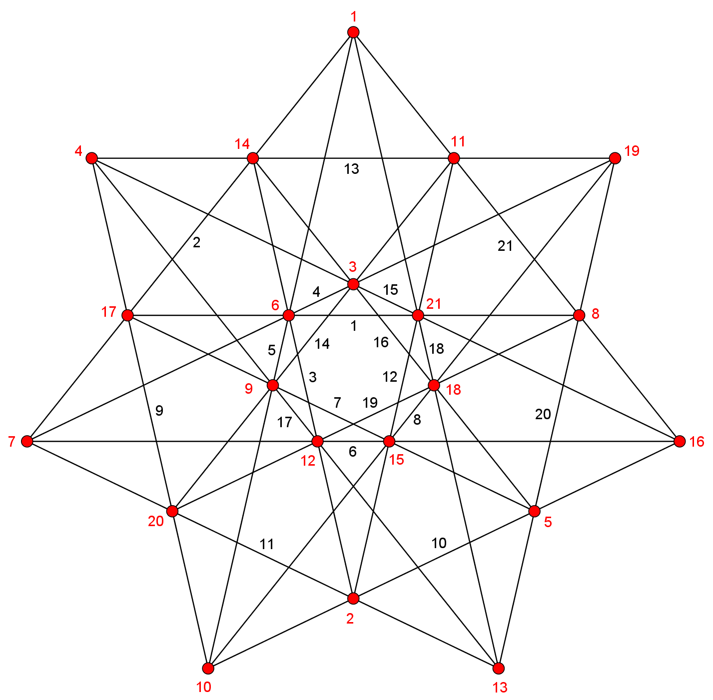
Figure 1: The $(21_{4})$ Grünbaum–Rigby configuration. The labels of points and lines are the same as those used above for the quadruple points and for the lines of $\mathcal{K}$, respectively.

It is known that the combinatorial symmetry of $\mathrm{GR}(21_{4})$ is inherited from $\Phi_{4}$, i.e. its automorphism group is equal to $G$ [7, 15]. On the other hand, its geometric symmetry group is isomorphic to the dihedral group $\mathrm{D}_{7}$. Both the set of points and the set of lines decomposes into three orbits under the action of this group. Moreover, two lines from each of two orbits of lines pass through each point, and two points from each of two orbits of points lie on each line. With these symmetry properties, this configuration belongs to the class of 3-astral, or, with the more recent term, 3-celestial configurations [14, 2].

A further interesting geometric symmetry property of $\mathrm{GR}(21_{4})$ is that it is perfectly self-reciprocal. We introduce this term for the property that there is a suitable circle $\Gamma$ such that the polar reciprocity with respect to $\Gamma$ transforms the configuration into itself; this property can be viewed as a strong version of self-duality. We note that reciprocity with respect to a circle $\Gamma$ is meant here in the classical sense as it is defined e.g. by Coxeter and Greitzer [8, Section 6.1].

To find the circle of reciprocity, in the particular case of $\mathrm{GR}(21_{4})$, one proceeds as follows. Due to the 7-fold rotational symmetry, there are three orbits of points, each having a circumcircle; similarly, there are three orbits of lines, each having an incircle. Consider now the outermost point orbit and the innermost line orbit. Construct the midcircle of the respective circumcircle and the incircle, i.e. the circle $\Gamma$ which determines an inversion swapping the given circumcircle and incircle. Doing the same for the pair of the innermost circumcircle and the outermost incircle, one finds that their midcircle is the same as before; moreover, the same circle $\Gamma$ serves also as the midcircle belonging to the third pair of point orbit and line orbit. Finally, it is checked that the set of points and lines of the configuration decomposes into pairs of pole and polar with respect to $\Gamma$.

2.3 Additional real point-line configurations derived form $\mathcal{K}$

It turns out that the configuration $K^{\prime}(12_{3})$ given in Proposition 2.1 can be realized as a geometric point-line configuration over the real numbers. This realization is shown in Figure 2. The labels of the lines refer to the set (1), and the labels of the points correspond to the notation of points of $\mathcal{K}$. This labelling verifies the isomorphism of this configuration to $K^{\prime}(12_{3})$, hence it is indeed a realization of $K^{\prime}(12_{3})$.

Observe that in Figure 2 four additional triple intersection points occur, namely those of the triples of lines labelled as (7,11,13), (3,8,14), (4,10,17) and (6,9,16). These extra points of intersection do indeed exist in this realization (but not in $\mathcal{K}^{\prime}$), and adding them to the the structure one obtains a real point-line $(16_{3},12_{4})$ configuration. This latter configuration is known as the dual of a configuration described by Zacharias who associated it to an incidence theorem [23, 11].

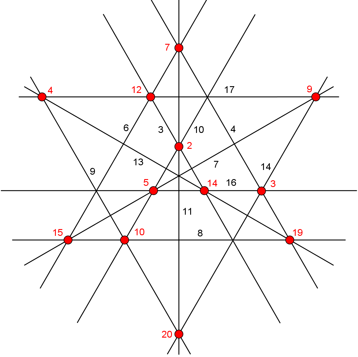
Figure 2: The real $(12_{3})$ point-line configuration derived from $\mathcal{K^{\prime}}$.

Remark 2.3.

It is worth emphasizing that the Zacharias configuration of points and lines, considered as an arrangement of lines, has exactly $19$ triple intersection points, the maximal possible number of such singular points for $12$ real lines. Moreover, this configuration has been rediscovered recently in [5], where we can find a complete classification of arrangements with $12$ pseudolines and $19$ triple points.

In what follows we use certain double points of the lines of $\mathrm{GR}(21_{4})$. As mentioned in the previous subsection, these lines form three orbits under the action of the $\mathrm{D}_{7}$ symmetry group of $\mathrm{GR}(21_{4})$. We take double points which are intersections of two lines belonging to different orbits. Accordingly, we have three orbits of such points, each consisting of 14 points. Obviously, they are located on three concentric circles, with radii $r_{1}<r_{2}<r_{3}$; we denote them by $O^{(1)}_{14}$, $O^{(2)}_{14}$ and $O^{(3)}_{14}$, respectively. Taking them in pairs, we have three different 28-element point sets. It turns out that in each of these sets there are 21 quadruples of collinear points. We add to each 28-element point set the lines lying on these quadruples; in this way we obtain three different point-line configurations of type $(28_{3},21_{4}$). We denote them by $\mathrm{GR}_{\mathrm{d}12}(28_{3},21_{4})$, $\mathrm{GR}_{\mathrm{d}23}(28_{3},21_{4})$ and $\mathrm{GR}_{\mathrm{d}13}(28_{3},21_{4})$, where the subscripts refer to the pairs of point orbits used in the construction. These configurations are depicted in Figures 3(a), 4(a) and 5(a), respectively.

Remark 2.4.

The numerical coincidence in the parameters suggests that some of the configurations $\mathrm{GR}_{\mathrm{d}12}(28_{3},21_{4})$, $\mathrm{GR}_{\mathrm{d}23}(28_{3},21_{4})$, or $\mathrm{GR}_{\mathrm{d}13}(28_{3},21_{4})$ is possibly isomorphic to the configuration consisting of the 21 lines and 28 triple points of the Klein arrangement. However, we could not establish such an isomorphism. Closer examination shows that there are many further point-line $(28_{3},21_{4})$ configurations over $\mathbb{R}$ different from those above, so we hope that continuing this work we shall be able to find such a real representation.

Now we take a circle concentric with $\mathrm{GR}_{\mathrm{d}12}(28_{3},21_{4})$, and produce the polar reciprocal $\mathrm{GR}_{\mathrm{d}12}(28_{3},21_{4})^{\vee}$ with respect to this circle. This is obviously a $(21_{4},28_{3})$ configuration. By scaling the circle of reciprocity appropriately, we obtain the surprising result that the union $\mathrm{GR}_{\mathrm{d}12}(28_{3},21_{4})\cup\mathrm{GR}_{\mathrm{d}12}(28_{3},21_{4})^{\vee}$ forms a $(49_{4})$ configuration (see Figure 3( b). We note that this latter configuration is not simply a union of $\mathrm{GR}_{\mathrm{d}12}(28_{3},21_{4})$ and its reciprocal, since new incidences occur here; actually, it is an incidence sum, as this notion is defined in [4]. Thus, when we speak about an appropriate scaling of the circle of reciprocity, this means that we change its radius until each point of the one configuration will be incident with a corresponding line of the other configuration, and vice versa.

A direct consequence of this construction is that our new configuration is perfectly self-reciprocal.

The same procedure can be applied to the two other configurations $\mathrm{GR}_{\mathrm{d}23}(28_{3},21_{4})$ and $\mathrm{GR}_{\mathrm{d}13}(28_{3},21_{4})$ as well. In this way, we obtain again perfectly self-reciprocal configurations. We denote these three self-reciprocal examples by $\mathrm{GR}_{\mathrm{d}12}(49_{4})$, $\mathrm{GR}_{\mathrm{d}23}(49_{4})$ and $\mathrm{GR}_{\mathrm{d}13}(49_{4})$, respectively. They are depicted in the (b) part of Figures 3, 4 and 5.

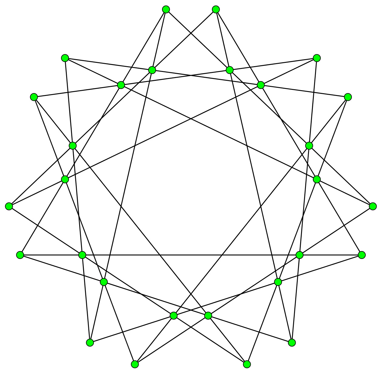
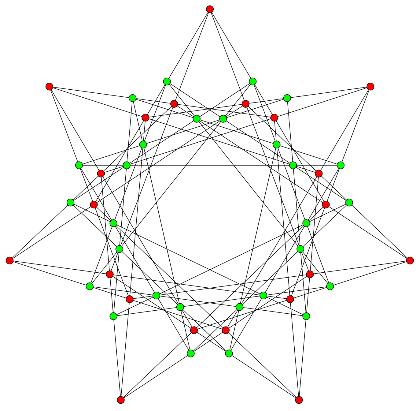
Figure 3: The configuration $\mathrm{GR}_{\mathrm{d}12}(28_{3},21_{4})$ (a) and the incidence sum with its polar reciprocal producing $\mathrm{GR}_{\mathrm{d}12}(49_{4})$ (b).

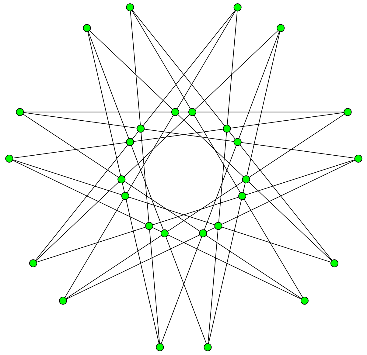
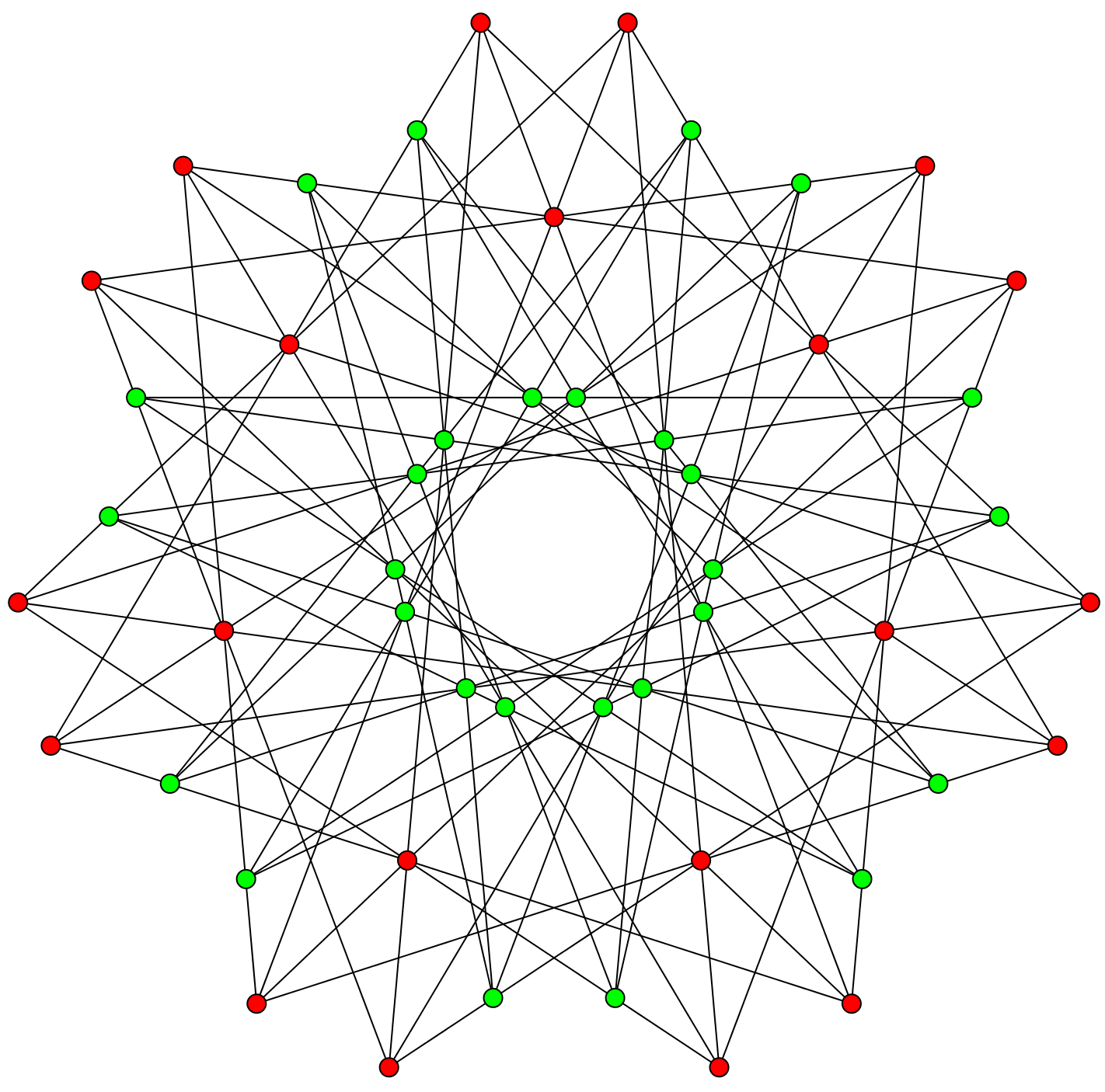
Figure 4: The configuration $\mathrm{GR}_{\mathrm{d}23}(28_{3},21_{4})$ (a) and the incidence sum with its polar reciprocal producing $\mathrm{GR}_{\mathrm{d}23}(49_{4})$ (b).

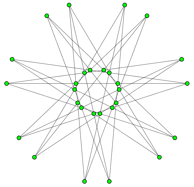
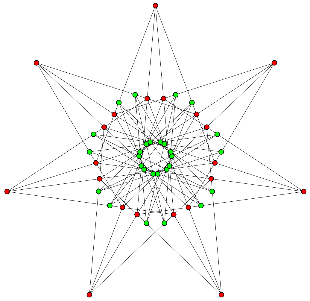
Figure 5: The configuration $\mathrm{GR}_{\mathrm{d}13}(28_{3},21_{4})$ (a) and the incidence sum with its polar reciprocal producing $\mathrm{GR}_{\mathrm{d}13}(49_{4})$ (b).

Finally, from the orbits $O^{(1)}_{14}$, $O^{(2)}_{14}$ and $O^{(3)}_{14}$, we can take one half of them such that each forms in itself a 7-orbit, this time under the action of the rotation group $\mathrm{C}_{7}$. Combining these 21 points with the quadruple points of $\mathrm{GR}(21_{4})$, one observes that collinear sixtuples of points occur (with appropriate choice of the halved orbits). Thus using the corresponding lines, one obtains a $(42_{4},28_{6})$ configuration. It is not clear whether it has a closer relationship with the nodes forming the orbit $\mathcal{O}_{42}$ mentioned in Proposition 3.1 below.

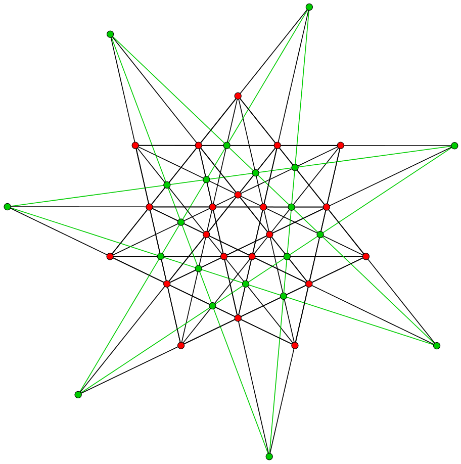
Figure 6: A real point-line $(42_{4},28_{6})$ configuration derived from $\mathcal{K}$.

2.4 On the rigidity of Klein’s arrangement of lines

Based on our experience regarding the Klein arrangement and Grünbaum-Rigby configuration, we would like to present here a short comparison between these two constructions. We point out here some discrepancies that might explain better why these object should be considered (geometrically) separately.

We start with the Klein arrangement. The main combinatorial object that can be associated with a line arrangement $\mathcal{A}$ (or hyperplanes, in general) is the intersection lattice $L(\mathcal{A})$ which consists of all intersections of elements of $\mathcal{A}$, including the ambient space as the empty intersection. Now we are going to define the notion of the moduli space associated with arrangements – we will follow Cuntz’s approach presented in [9]. Let $\mathbb{K}$ be a field and denote by $\mathcal{A}=\{H_{1},...,H_{d}\}$ a central hyperplane arrangement in $\mathbb{K}^{3}$. Here by a central arrangement we mean that all hyperplanes pass through the origin and, due to this reason, the projectivization of $\mathcal{A}$ is an arrangement of lines in $\mathbb{P}^{2}_{\mathbb{K}}$. For a matrix $M=[m_{1},...,m_{d}]\in M_{3\times d}(\mathbb{K})$ we attach a central hyperplane arrangement $\mathcal{B}_{M}=\{H_{i}^{{}^{\prime}}={\rm ker}(m_{i})\,:\,i\in\{1,...,d\}\}\setminus\mathbb{K}^{3}$ that sits in $\mathbb{K}^{3}$. Now we consider the following condition for $M$:

$$(\ast) |\mathcal{B}_{M}|=d\text{ and there exists an isomorphism }\pi\colon L(\mathcal{A})\rightarrow L(\mathcal{B}_{M})$$

$$\text{ of graded lattices such that }\pi(H_{i})=H_{i}^{\prime}\text{ for }1\leq i\leq d.$$

For a lattice $L$ on $\{1,\ldots,d\}$, we define

$$\mathcal{U}(L)=\{M\in M_{3\times d}(\mathbb{K})\,:\,M\text{\ satisfies\ }(\ast)\}.$$

Since the condition ($\ast$) is determined by vanishing / non-vanishing of minors in $M$, it follows that $\mathcal{U}(L)$ has a structure of an algebraic variety. We define the moduli space $\mathcal{V}_{\mathbb{K}}(L)$ of arrangements whose intersection lattice is $L$ as

$$\mathcal{V}_{\mathbb{K}}(L):={\rm PGL}(3,\mathbb{K})\backslash(\mathcal{U}(L)/(\mathbb{K}^{*})^{d}).$$

For a lattice $L$, we write ${\rm Aut}(L)$ for the set of automorphisms of posets, i.e., the set of bijections preserving the relations in the poset.

In order to understand the moduli space of the Klein arrangement of lines, we will need one additional definition.

Definition 2.5.

Let $L$ be the intersection lattice of a central hyperplane arrangement $\mathcal{A}\subset\mathbb{K}^{3}$. We call one dimensional elements as points, and the two dimensional elements as lines (this abusing comes from the projectivization of $\mathcal{A}$). We say that lines $H_{1},...,H_{n}$ in $L$ generate $L$ if there is a sequence of points and lines $U_{1},...,U_{m}$ in $L$ such that:

1. $U_{i}=H_{i}$ for all $i\in\{1,...,n\}$,

2. For all $i>n$ there exist $j,k<i$ such that $U_{i}\in\{U_{j}\cap U_{k},U_{j}+U_{k}\}$,

3. Every line of $L$ is contained in $\{U_{1},...,U_{m}\}$.

Furthermore, we define

$$g(L):={\rm min}\{n\in\mathbb{N}\,:\,L\text{ is generated by }n\text{ lines}\}.$$

In other words, our intersection lattice is generated by lines $H_{1},...,H_{n}$ if all the lines in $L$ are obtained by inductively adding intersection points of two lines, or lines through two points.

Based on the above introduction, we can show the following.

Theorem 2.6.

The Klein arrangement $\mathcal{K}$ is a rigid arrangement, i.e., it is unique up to the projective equivalence.

Remark 2.7.

The fact that the Klein arrangement is rigid in somehow well-known in folklore. However, we were not able to detect any direct reference towards this property in the literature, and that is the reason why we decided to discuss this issue here.

Proof.

Since our proof of this claim is computer-assisted, based on algorithm [9, Algorithm 3.9] due to Cuntz, we present an outline. As an input, we take a matroid $L$ of rank three and a field $\mathbb{C}$. The output of the algorithm is a pair of algebraic varieties $V,E$ such that $\mathcal{V}_{\mathbb{C}}(L)=V\setminus E$. We have three steps, in the first one we need to choose a set of generating lines $G:=\{H_{1},...,H_{n}\}$ of $L$. Then for a largest subset $S\subset G$ of $G$ in general position, one chooses basis elements of $\mathbb{C}^{3}$ as coordinate vectors and for the remaining $d:=|G\setminus S|$ lines in $G\setminus S$ one chooses coordinate vectors consisting of variables in a polynomial ring $\mathbb{C}[x_{1},...,x_{3d}]$. Since every triple of lines in $L$ gives a condition on the determinant of the corresponding vectors as coordinates, yielding varieties $V$ and $E$ as required depending on whether the determinant is zero or not. According to what we have seen so far, we need to find a set of generating lines. It turns out, based on computer calculations, that for the intersection poset $L$ of the Klein arrangement $\mathcal{K}$ we have

$$g(L)=5$$

and the generating lines can be chosen as follows (here we use equations of lines presented in Section 2.1):

$$H_{1} :\,x=0,$$

$$H_{2} :\,y=0,$$

$$H_{3} :\,z=0,$$

$$H_{4} :\,x-(a+1)y-z=0,$$

$$H_{5} :\,x-y+(a+1)z=0.$$

Following the path of the algorithm, we can check that indeed the presentation of the Klein arrangement is unique up to projectivities and conjugates. ∎

Remark 2.8.

It was announced in [9, Example 3.2] that for reflection arrangements $\mathcal{A}$ associated with irreducible complex reflection groups of rank three the moduli spaces $\mathcal{V}_{\mathbb{C}}(L(\mathcal{A}))$ are finite and these finitely many realizations of $L(\mathcal{A})$ in $\mathcal{V}_{\mathbb{C}}(L(\mathcal{A}))$ are Galois conjugate under automorphisms of the smallest field extension of $\mathbb{Q}$ over which $L(\mathcal{A})$ is realizable. This explains, in particular, that the Wiman arrangement of $45$ lines with $120$ triple, $45$ quadruple, and $36$ quintuple points is unique up to the projective equivalence.

2.5 An incidence conjecture for $\mathrm{GR}(21_{4})$

Observe that $\mathrm{GR}(21_{4})$ is the union of three subconfigurations of type $(14_{2},7_{4})$ (see Figure 7). The set of points of the first subconfiguration, which we denote by $\mathrm{S}_{12}$, is composed of the outermost and the intermediate point orbit of $\mathrm{GR}(21_{4})$; we denote these orbits by $\mathrm{P}_{1}$ and $\mathrm{P}_{2}$, respectively. Its lines form the side lines of a regular star-heptagon of type $\big{\{}\frac{7}{2}\big{\}}$ (for this notation, see Coxeter [6]). The second and the third subconfiguration, denoted by $\mathrm{S}_{13}$ and $\mathrm{S}_{23}$, have $\mathrm{P}_{1}\cup\mathrm{P}_{3}$ and $\mathrm{P}_{2}\cup\mathrm{P}_{3}$ as set of points, respectively, where $\mathrm{P}_{3}$ denotes the innermost point orbit of $\mathrm{GR}(21_{4})$. The lines of both these subconfigurations form the side lines of a regular star-heptagon of type $\big{\{}\frac{7}{3}\big{\}}$. Thus they are isomorphic to each other, but are non-isomorphic to $\mathrm{S}_{12}$.

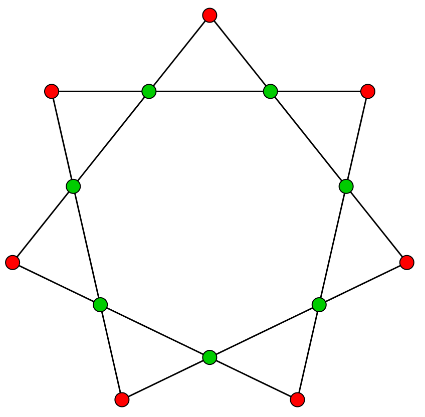
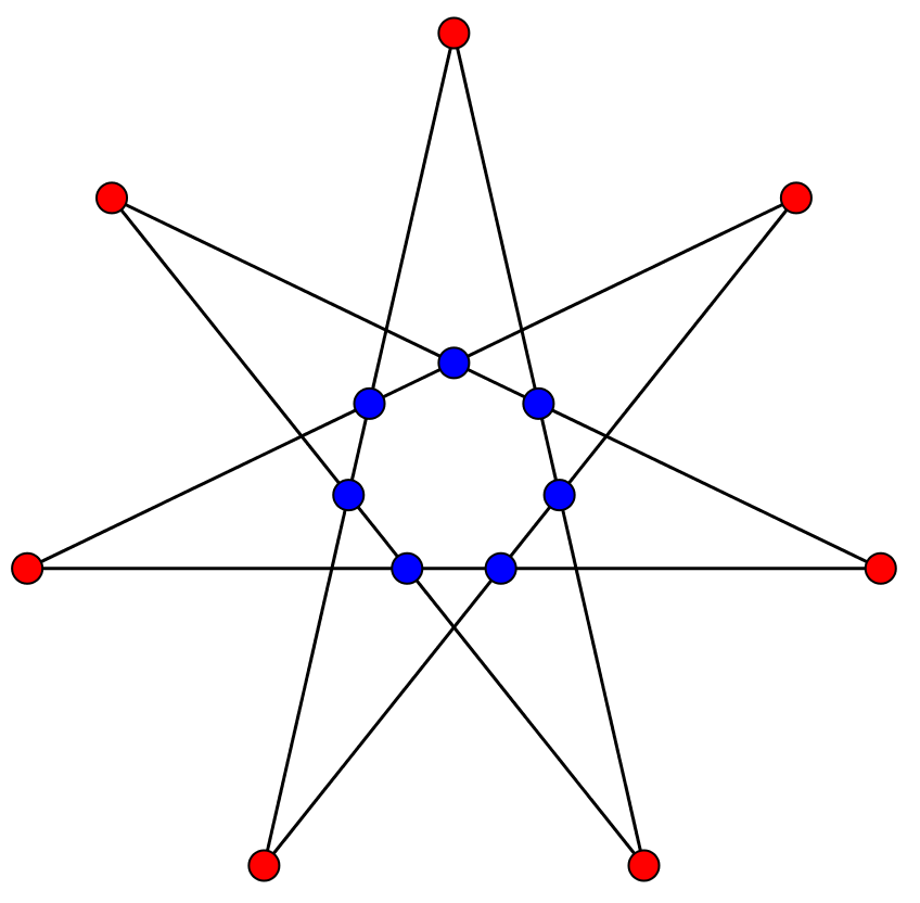
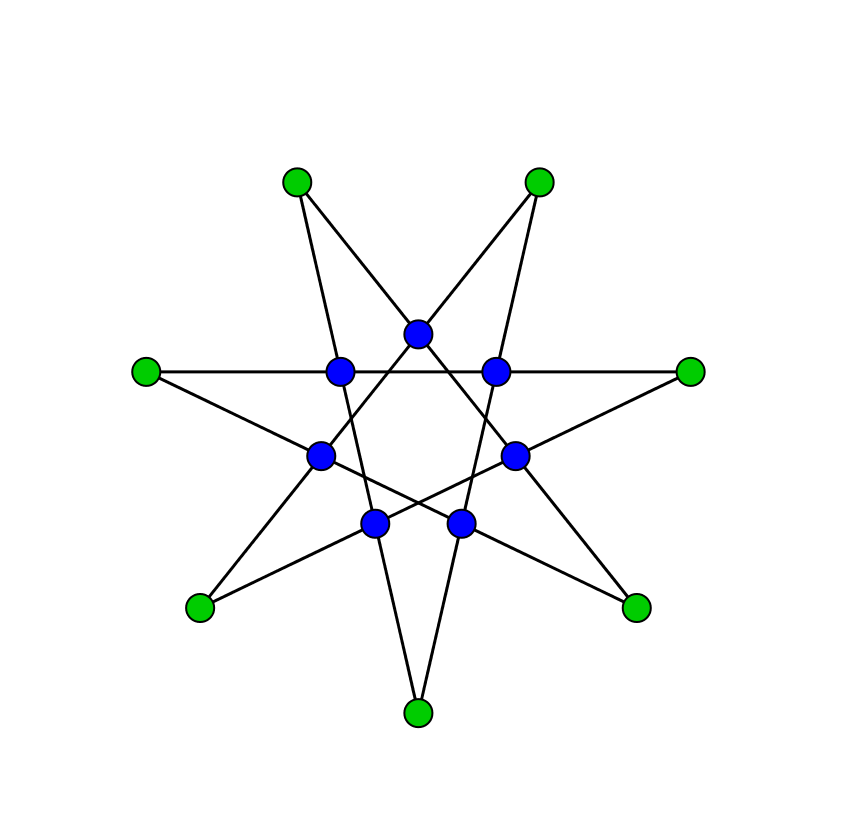
Figure 7: Subconfigurations of type $(14_{2},7_{4})$ in the Grünbaum–Rigby configuration. Left: $\mathrm{S}_{12}$. Centre: $\mathrm{S}_{13}$. Right: $\mathrm{S}_{23}$. The point orbits $\mathrm{P}_{1}$, $\mathrm{P}_{2}$, $\mathrm{P}_{3}$ are denoted by different colours.

Now consider three configurations $\mathrm{S}^{\prime}_{12}$, $\mathrm{S}^{\prime\prime}_{13}$, and $\mathrm{S}^{\prime\prime\prime}_{23}$, such that the following isomorphisms hold:

$$\varphi_{1}:\mathrm{S}^{\prime}_{12}\rightarrow\mathrm{S}_{12};\quad\varphi_{2}:\mathrm{S}^{\prime\prime}_{13}\rightarrow\mathrm{S}_{13};\quad\varphi_{3}:\mathrm{S}^{\prime\prime\prime}_{23}\rightarrow\mathrm{S}_{23}.$$

Under this correspondence, the point sets of the three new configurations are:

$$\mathrm{P}^{\prime}_{1},\mathrm{P}^{\prime}_{2}\subset\mathrm{S}^{\prime}_{12};\quad\mathrm{P}^{\prime\prime}_{1},\mathrm{P}^{\prime\prime}_{3}\subset\mathrm{S}^{\prime\prime}_{13};\quad\mathrm{P}^{\prime\prime\prime}_{2},\mathrm{P}^{\prime\prime\prime}_{3}\subset\mathrm{S}^{\prime\prime\prime}_{23}.$$

We have the following conjecture.

Conjecture 2.9.

Suppose that the point set $\mathrm{P}^{\prime}_{1}$ is inscribed in a conic $C_{1}$, and the point set $\mathrm{P}^{\prime}_{2}$ is inscribed in a conic $C_{2}$. Then $\mathrm{S}^{\prime}_{12}$, $\mathrm{S}^{\prime\prime}_{13}$, and $\mathrm{S}^{\prime\prime\prime}_{23}$ can be chosen in such a way that their union forms a configuration isomorphic to $\mathrm{GR}(21_{4})$, where

• $\mathrm{P}^{\prime}_{1}$ is identified with $\mathrm{P}^{\prime\prime}_{1}$,

• $\mathrm{P}^{\prime}_{2}$ is identified with $\mathrm{P}^{\prime\prime\prime}_{2}$,

• $\mathrm{P}^{\prime\prime}_{3}$ is identified with $\mathrm{P}^{\prime\prime\prime}_{3}$;

moreover, $\mathrm{P}^{\prime\prime}_{3}=\mathrm{P}^{\prime\prime\prime}_{3}$ is inscribed in a conic $C_{3}$.

Remark 2.10.

$\mathrm{S}^{\prime}_{12}$ does not play a distinguished role in the statement above. In fact, it can be replaced either by $\mathrm{S}^{\prime\prime}_{13}$ or by $\mathrm{S}^{\prime\prime\prime}_{23}$ (followed by appropriate cyclic permutation of these subconfigurations).

Loosely speaking, the conjecture tells us that the shape of the Grünbaum–Rigby configuration can change in such a way that if both its outermost and intermediate point heptad have a circumconic, then its third point heptad also has a circumconic. Figure 8 shows an example of such a general shape, together with the circumconics.

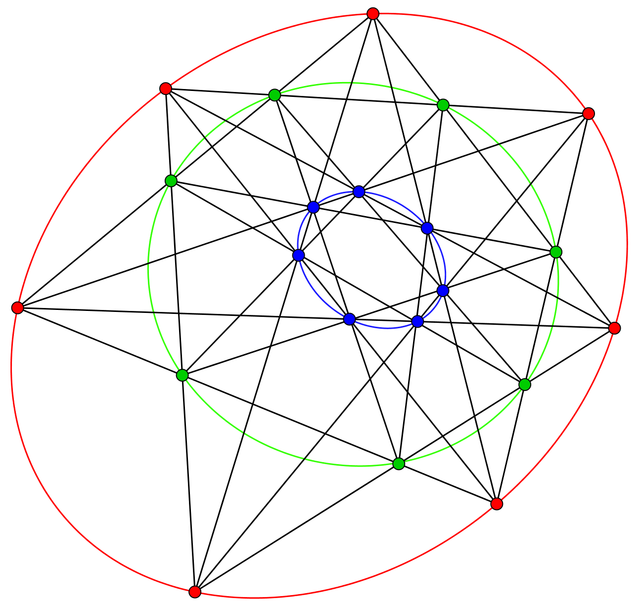
Figure 8: Illustration for Conjecture 2.9.

So far, we have no proof of this conjecture, but by use of dynamic geometry software, we have experimental evidence. In particular, such experiments show that there are infinitely many projectively inequivalent versions of this configuration. This means that if the conjecture is true, then it implies movability of the Grünbaum–Rigby configuration (by the definition given by Grünbaum [14, Section 5.7]). In the forthcoming section we deliver an evidence for this claim via the geometry of the moduli space of a certain Grünbaum–Rigby arrangement.

2.6 On the moduli space of a Grünbaum–Rigby arrangement

Our prediction, based on computer algebra experiments, tells us that the Grünbaum–Rigby configuration has to be movable in the sense of Grünbaum. By the comments of the referee, which we really appreciate, our aim is to understand one component of the moduli space of realizations of the the Grünbaum–Rigby configuration. In order to do so, we have to fix the whole intersection poset, i.e., this is not only about the incidences between quadruple points and lines, but we also fix other intersection points. More precisely, there exists a geometric realization of a Grünbaum–Rigby configuration that has exactly $21$ quadruple points and $84$ double points. This realization, denoted here by $\mathcal{GR}$, form an arrangement of $21$ lines, and our aim is to proceed our computations for this object. It is worth pointing our here that, by selecting this particular geometric realization, we will find a component of the moduli space parametrizing all possible geometric realization of the intersection poset that we present below. Let us present the incidences that allow us to construct a rank $3$ matroid that is representable over the real and it is associated to $\mathcal{GR}$ – here $[a,b,c,d]$ means that we have a quadruple points being an intersection of lines labeled by $a,b,c,d$.

$$\mathcal{I}_{\mathcal{GR}}=\bigg{\{}[1,2,15,21],[1,3,8,13],[1,6,9,14],[4,5,15,16],[4,6,8,10],[8,11,15,18],[9,13,17,21],\\ [11,14,16,20],[2,4,9,11],[9,12,15,19],[3,5,12,14],[8,12,17,20],[10,13,16,19],[3,4,17,18],\\ [2,3,19,20],[10,14,18,21],[1,7,16,17],[5,6,20,21],[5,7,11,13],[2,7,10,12],[6,7,18,19]\bigg{\}}.$$

Based on the data $\mathcal{I}_{\mathcal{GR}}$ we construct a rank $3$ matroid for which we compute the moduli space. To do this, we followed the algorithmic setup described in [1]. Consider a $3\times n$ matrix $A$ of $3n$ variables $x_{i,j}$ in $\mathbb{C}[x_{i,j}\mid 1\leq i\leq 3,1\leq j\leq n]$. Then let $I$ be the ideal of all $3\times 3$ minors of $A$ corresponding to triples of lines intersecting in a point. Similarly, let $J$ be the set of all $3\times 3$ minors of $A$ corresponding to triples of lines that do not intersect in a point. The moduli space is then $V(I)\setminus\bigcup_{p\in J}V(p)$ as an affine variety in $\mathbb{C}^{3n}$. To obtain the moduli space of arrangements up to projective equivalences, one can set certain values of the matrix $A$ to $0$ or $1$ depending on the combinatorics of the arrangement (cf. [1] for details). It turns out that the component of the moduli space is a Zariski open set of $\mathbb{P}^{3}_{\mathbb{C}}$, but the precise description of this set is rather involving and we have to omit it here. In that spot we would like to warmly thank L. Kühne for his help with involving computations.

3 Klein’s arrangements of conics

3.1 Polars to the Klein quartic

Now we would like to construct, using two different methods, Klein arrangements consisting of smooth conics. The first construction, the classical one, dates back to Gerbaldi in 1882 [10], and it is based on the so-called polars to the Klein quartic curve. Now we are going to explain how to extract from this construction $21$ conics.

We start with the notion of the Steinerian curve which is the locus of points $p$ such that the polar to a given curve $C$ with respect to $p$ is singular. By Bertini [3], the Steinerian of a general quartic curve has $21$ nodes and $24$ cusps. Recall that the Steinerian curve is invariant under the action of $G$ and the set of $21$ nodes forms an orbit $\mathcal{O}_{21}$ of the length $21$. Moreover, since the Steinerian curve is an invariant curve of degree $12$, it must be a linear combination of $\Phi_{4}^{3}$ and $\Phi_{6}^{2}$. One can observe that the only linear combination of these forms which vanishes at $\mathcal{O}_{21}$ is $4\Phi_{4}^{3}+\Phi_{6}^{2}$, so this is the equation of the Steinerian.

It turns out that each polar to $\Phi_{4}$ with respect to each point $p\in\mathcal{O}_{21}$ splits as a smooth conic and a line meeting transversely at two points. Now we explain how to achieve this goal.

Consider the following gradient map $\nabla(\Phi_{4})$ given by the partial derivatives of the Klein quartic equation

$$\mathbb{P}^{2}_{\mathbb{C}}\ni(x:y:z)\xrightarrow{9:1}(u:v:w)=(3x^{2}y+z^{3}:3y^{2}z+x^{3}:3z^{2}x+y^{3})\in\mathbb{P}^{2}_{\mathbb{C}}.$$

By definition, the polar $P_{p}(\Phi_{4})$ with respect to the point $p=(a:b:c)\in\mathbb{P}^{2}_{\mathbb{C}}$ is the preimage under $\nabla(\Phi_{4})$ of the line dual to $p$, $V(au+bv+cw)\subset\mathbb{P}^{2}_{\mathbb{C}}$. Since the Klein quartic is non-singular, the partial derivatives never vanish, so the gradient map is defined everywhere. We can sum up the most important features of the obtained arrangement of conics and lines – see [20, Proposition 2.1].

Proposition 3.1.

The Klein quartic $\Phi_{4}$ has exactly $21$ reducible polars and each consists of a line and a conic meeting transversely at two points. They are the polars with respect to the $21$ quadruple points of $\Phi_{21}$. The $21$ lines which are components of the reducible polars are also the components of $\Phi_{21}$, whereas each of the $21$ conics intersect the Klein curve at the eight points of contact of four bitangents. The nodes of the $21$ reducible polars are all distinct and form the orbit $\mathcal{O}_{42}$.

Extracting the $21$ conics from the above, we have the following observation.

Proposition 3.2.

The arrangement $\mathcal{K}_{2}$ consisting of the $21$ smooth conics extracted from the $21$ reducible polars has only transversal intersection points as the singularities, namely $224=8\cdot 21+56$ triple and $168=21\cdot 8$ double points.

We can find the equations of $21$ conics using the following Singular script - we hope that this might be useful to the reader who wants to use these conics for different purposes.

ring R=(0,e),(x,y,z),dp;
minpoly=e6+e5+e4+e3+e2+e+1;
poly Phi4=x3y+y3z+z3x;
ideal jf=jacob(Phi4);
poly Phi6=-det(jacob(jf))/54;
ideal jfh=jf+ideal(Phi6);
matrix bh[4][4]=transpose(jacob(jfh)),jacob(Phi6);
poly Phi14=det(bh)/9;
poly Phi21=det(jacob(ideal(Phi4,Phi6,Phi14)))/14; // the equation of lines
map f=R,jacob(Phi4);
poly Phi63=f(Phi21);
poly Phi42=Phi63/Phi21;
factorize(Phi42); // the equations of conics

Remark 3.3.

Based on the construction presented above, we dare to call the arrangement $\mathcal{K}_{2}$ as a polar Klein arrangement of smooth conics.

3.2 The dual curve to the Klein quartic and an associated conic arrangement

Now we pass to the second construction that was presented by Roulleau [21]. This construction is based on the dual curve $\check{C}$ to the Klein quartic curve. It is known that the degree of $\check{C}$ is $12$, since the Klein quartic curve is smooth, and we verify by Plücker formulae that $\check{C}$ has $52$ singular points, i.e., it has exactly $28$ nodes $\mathcal{P}_{28}$ corresponding to the $28$ bitangents and $24$ cusps $\mathcal{P}_{24}$ corresponding to the $24$ flex points of the quartic.

One can check, using computer software like Singular, that there exists a set of $21$ conics passing through exactly $8$ element subsets of the set $\mathcal{P}_{28}$, and through each point of $\mathcal{P}_{28}$ there are $6$ conics passing through them. It means, we obtained a $(28_{6},21_{8})$ point-conic configuration. One can also check that these $21$ conics, considered as an arrangement of curves, has additionally $420$ double intersection points. One can easily check that there are no other singular points via the following combinatorial count

$$840=4\cdot\binom{21}{2}=\sum_{r\geq 2}\binom{r}{2}t_{r}=t_{2}+\binom{6}{2}t_{6}=420+15\cdot 28.$$

Proposition 3.4 (Roulleau).

There exists a set of $21$ smooth conics determined by the set $\mathcal{P}_{28}$ of all nodes of the dual curve $\check{C}$ to the Klein quartic $\Phi_{4}$. These $21$ conics form an arrangement having $28$ sixtuple points and $420$ double intersection points.

Because the defining equation of the above conic arrangement is quite complicated, we skip it here and refer to [22] for necessary computations performed by X. Roulleau in MAGMA.

3.3 Real point-conic configurations derived from $\mathcal{K}$

One can derive two different $(21_{7})$ point-conic configurations from the Grünbaum–Rigby configuration in such a way that conics are circumscribed on 7-tuples of points of $\mathrm{GR}(21_{4})$ [11]. One of them has the special combinatorial property that it is resolvable, which means that the set of conics can be partitioned into 7 classes (called resolution classes) such that within each class the conics partition the point set of the configuration [11, Figure 5] (we note that the configuration $K^{\prime}(12_{3})$ described in Section 2.3 is also resolvable). This particular version is interesting in the light of our Conjecture 2.9. Experiments show that when applying the circumconics of the conjecture and destroying the original $\mathrm{D}_{7}$ symmetry, the conics circumscribed on the point 7-tuples of the configuration are preserved as circumconics; as a result, added the three new conics, we have a movable $(21_{8},24_{7})$ point-conic configuration (provided the conjecture is true).

A class of point-conic configurations can be derived from the point-line $\mathrm{GR}_{\mathrm{d}12}(28_{3},21_{4})$ configuration presented in Section 2.3. Taking suitable 8-element subsets of points of this configuration, one can circumscribe 28 conics on them. In this way we obtain a $(28_{8})$ point-conic configuration (see Figure 9).

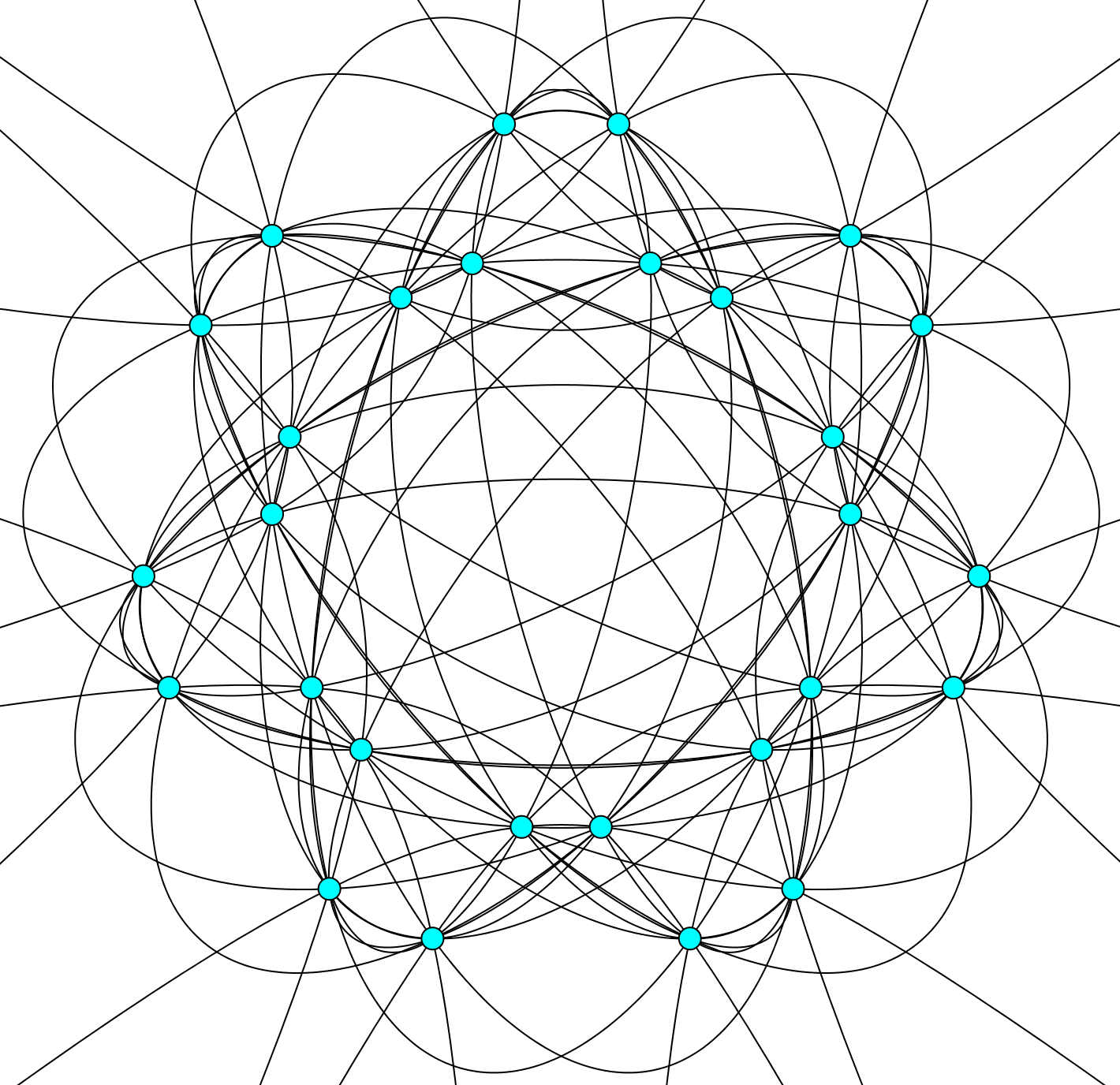
Figure 9: A point-conic $(28_{8})$ configuration derived from the point-line configuration $\mathrm{GR}_{\mathrm{d}12}(28_{3},21_{4})$.

The set of conics of this configuration decomposes into four orbits under the action of the $\mathrm{D}_{7}$ geometric symmetry group of $\mathrm{GR}_{\mathrm{d}12}(28_{3},21_{4})$ (namely, three orbits of ellipses and one orbit of hyperbolas). Each orbit of conics forms a $(28_{2},7_{8})$ subconfiguration. A consequence of this combinatorial regularity of the distribution of points among the conics is that we have four distinct subconfigurations of type $(28_{6},21_{8})$; these are obtained by removing respectively one of the four orbits of conics. So far, it is not decided whether they are pairwise non-isomorphic. It is also subject to further investigation as to whether any of them is isomorphic to the complex $(28_{6},21_{8})$ configuration mentioned in the previous section.

An additional (balanced) point-conic configuration can be derived in an analogous way from the point-line configuration $\mathrm{GR}_{\mathrm{d}12}(49_{4})$ depicted in Figure 3(b). Its type is $(49_{8})$ (cf. Figure 10). It preserves the $\mathrm{D}_{7}$ geometric symmetry of the underlying point-line configuration; the set of conics is partitioned into 7 orbits (4 of ellipses and 3 of hyperbolas) under the action of this group. The distribution of the points among the conics is a little less regular then in the case above, so subconfigurations of type $(28_{2},7_{8})$ are provided only by three of these orbits (possibly with isomorphic pairs among them).

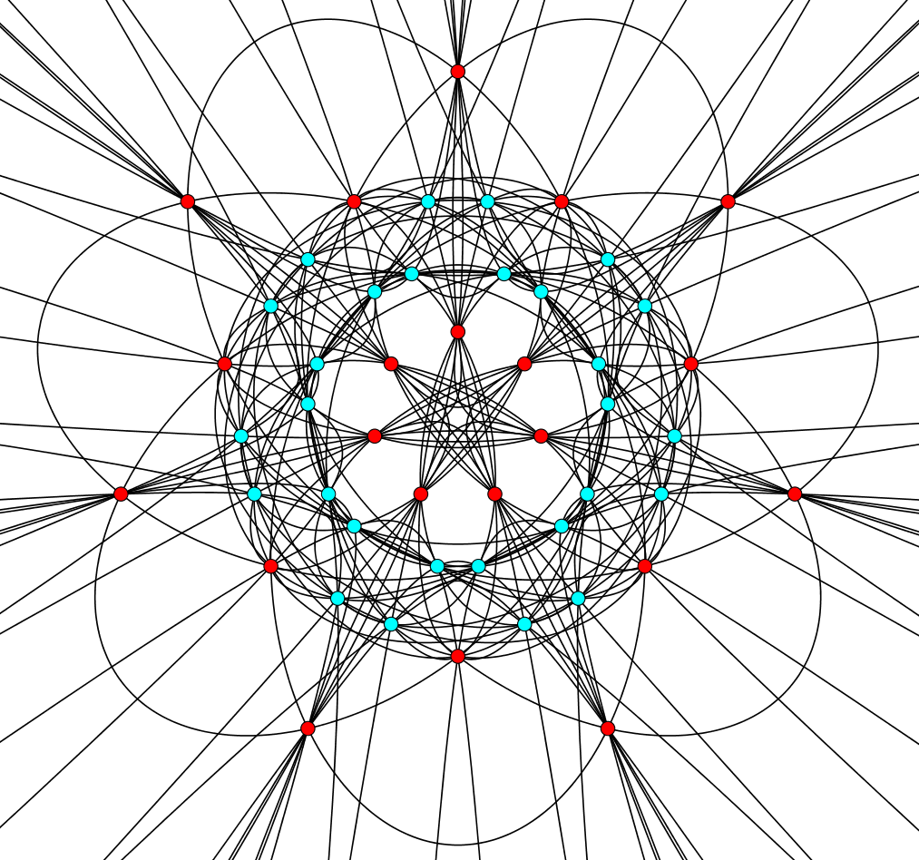
Figure 10: A point-conic $(49_{8})$ configuration derived from the point-line configuration $\mathrm{GR}_{\mathrm{d}12}(49_{4})$.

We note that from the non-balanced $(28_{2},7_{8})$ subconfigurations considered above, one can form 4-factor Cartesian products, including repeated use of any of the factors (for Cartesian products of point-conic configurations realized in plane, see [13]). These products form balanced $(614656_{8})$ configurations (where $614656=28^{4}$).

An additional product can be derived from the $(49_{8})$ configuration: omitting three suitably chosen orbits of conics and 21 points chosen accordingly, one obtains in the first step a $(28_{4},14_{8})$ subconfiguration (see Figure 11). Then, in the second step, we take the Cartesian square of this latter (non-balanced) configuration. This provides a balanced $(784_{8})$ configuration.

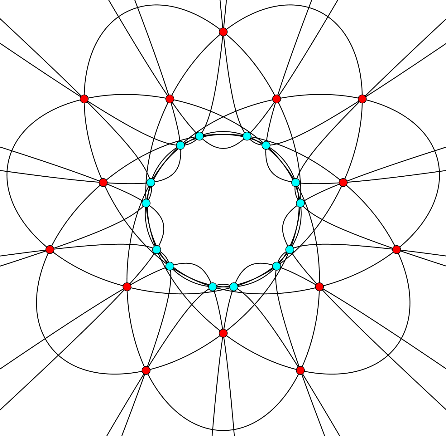
Figure 11: The $(28_{4},14_{8})$ subconfiguration of the point-conic $(49_{8})$ configuration.

Gábor Gévay
Bolyai Institute, University of Szeged
Aradi vértanúk tere 1, H-6720 Szeged, Hungary
E-mail address: gevay@math.u-szeged.hu
ORCID: https://orcid.org/0000-0002-5469-5165

Piotr Pokora
Department of Mathematics, Pedagogical University of Krakow
Podchora̧żych 2, PL-30-084 Kraków, Poland
E-mail address: piotr.pokora@up.krakow.pl
ORCID: http://orcid.org/0000-0001-8526-9831

References

- [1] M. Barakat and L. Kühne, Computing the nonfree locus of the moduli space of arrangements and Terao?s freeness conjecture, Math. Comp., 92 (2023), 1431–1452.
- [2] A. Berardinelli and L. W. Berman, Systematic celestial 4-configurations, Ars Math. Contemp., 7 (2014), 361–377.
- [3] E. Bertini, Le tangenti multiple della Cayleyana di una quartica piana generale, Atti Acad. Sci. Torino, 32 (1896), 32–33.
- [4] M. Boben, G. Gévay and T. Pisanski, Danzer’s configuration revisited, Adv. Geom. 15 (2015), 393–408.
- [5] J. Bokowski and P. Pokora, On the Sylvester-Gallai and the orchard problem for pseudoline arrangements, Period. Math. Hung., 77(2) (2018), 164–174.
- [6] H. S. M. Coxeter, Introduction to Geometry, Wiley, New York, 1961.
- [7] H. S. M. Coxeter, My graph, Proc. London Math. Soc. (3) 46 (1983), 117–136.
- [8] H. S. M. Coxeter and S. L. Greitzer, Geometry Revisited, The Mathematical Association of America, Washington, D.C., 1967.
- [9] M. Cuntz, A greedy algorithm to compute arrangements of lines in the projective plane. Discrete Comput. Geom. 68(1) (2022), 107–124.
- [10] F. Gerbaldi, Sul gruppi di sei coniche in involuzione, Atti Accad. Sci. Torino, 17 (1882), 566–580.
- [11] G. Gévay, Resolvable configurations, Discrete Appl. Math. 266 (2019), 319–330.
- [12] G. Gévay and T. Pisanski, Kronecker covers, -construction, unit-distance graphs and isometric point-circle configurations, Ars Math. Contemp., 7 (2014), 317–336.
- [13] G. Gévay, N. Bašić, J. Kovič and T. Pisanski, Point-ellipse configurations and related topics, Beitr. Algebra Geom. 63 (2022), 459–475.
- [14] B. Grünbaum, Configurations of Points and Lines, American Mathematical Society, Providence, Rhode Island, 2009.
- [15] B. Grünbaum and J. F. Rigby, The real configuration , J. London Math. Soc. 41 (1990), 336–346.
- [16] R. H. Jeurissen, C. H. van Os, J. H. M. Steenbrink, The configuration of bitangents of the Klein curve, Discrete Math. 132(1-3) (1994), 83–96.
- [17] F. Klein, Ueber die Transformationen siebenter Ordnung der elliptischen Funktionen, Math. Ann. 14 (3) (1878), 428–471.
- [18] A. M. Macbeath, Hurwitz groups and surfaces, in: S. Levy (ed.) The Eightfold Way: The Beauty of Klein’s Quartic Curve, MSRI Publicatons 35, Cambridge University Press, Cambridge, 1999.
- [19] T. Pisanski and B. Servatius, Configurations from a Graphical Viewpoint, Birkhäuser Advanced Texts, Birkhäuser, New York, 2013.
- [20] P. Pokora and J. Roé, The 21 reducible polars of Klein?s quartic, Exp. Math. 30 (2021), 1–18.
- [21] X. Roulleau, Conic configurations via dual of quartic curves, Rocky Mountain J. Math. 51 (2) (2021), 721–732.
- [22] X. Roulleau, Conic configurations via dual of quartic curves - ancillary file with the Magma computations, https://arxiv.org/src/2002.05681v2/anc/AllMagmaComputations.txt.
- [23] M. Zacharias, Untersuchungen über ebene Konfigurationen , Deutsche Math. 6 (1941) 147–170.