Statistical Majorana Bound State Spectroscopy
Abstract
Tunnel spectroscopy data for the detection of Majorana bound states (MBS) is often criticized for its proneness to misinterpretation of genuine MBS with low-lying Andreev bound states. Here, we suggest a protocol removing this ambiguity by extending single shot measurements to sequences performed at varying system parameters. We demonstrate how such sampling, which we argue requires only moderate effort for current experimental platforms, resolves the statistics of Andreev side lobes, thus providing compelling evidence for the presence or absence of a Majorana center peak.
Introduction.—About a decade after the first proposals for MBS engineering in topological quantum devices Alicea (2012); Leijnse and Flensberg (2012); Beenakker (2013); DasSarma, Freedman, and Nayak (2015), numerous reports of experimental signatures have been published, see, e.g., Refs. Mourik et al. (2012); Nadj-Perge et al. (2014); Lutchyn et al. (2018); Liu et al. (2018); Li et al. (2022); MicrosoftQuantum (2022). However, opinions remain divided as to whether “Majoranas have been seen” or not. Broadly speaking, experiments aimed at MBS detection can be categorized into two groups: tunnel spectroscopy detecting midgap resonances caused by the assumed presence of an MBS Sengupta et al. (2001); Law, Lee, and Ng (2009); Flensberg (2010); Sun et al. (2016); Zazunov, Egger, and Levy Yeyati (2016), and experiments going after unambiguous intrinsic properties of topological states, from unconventional noise correlations Bolech and Demler (2007); Nilsson, Akhmerov, and Beenakker (2008); Golub and Horovitz (2011); Haim et al. (2015); Liu, Cheng, and Lutchyn (2015); Tripathi, Das, and Rao (2016); Jonckheere et al. (2017, 2019); Manousakis et al. (2020) to full-feathered braiding protocols Aasen et al. (2016); Beenakker (2020); Flensberg, von Oppen, and Stern (2021); Sbierski et al. (2022). While the second group remains at the level of theoretical proposals, the former are straightforwardly realizable as a part of the core MBS experiments. However, the downside is that tunnel spectroscopy data can be prone to misinterpretation. Among various other candidates for midgap signatures, pairs of conventional Andreev bound states — which in symmetry class D Altland and Zirnbauer (1997); Beenakker (2015) superconductor environments111 Strictly speaking, the system is either in class B or in class D depending on whether a MBS is present or not. For simplicity, we refer to both cases as “class D”. have a tendency to cluster around zero energy — may leave experimental signatures hard to distinguish from a single MBS Bagrets and Altland (2012); Liu et al. (2012); Aguado (2017); Moore, Stanescu, and Tewari (2018); Vuik et al. (2019); Prada et al. (2020); Valentini et al. (2021); Yu et al. (2021). At any rate, as witnessed by the current debate on the “topological gap protocol” by the Microsoft Quantum team MicrosoftQuantum (2022); Frolov and Mourik (2022); Akhmerov (2022), the community at large does not appear to be ready to take tunnel spectroscopy signatures, even of high quality, as unambiguous evidence for MBS formation.
In this paper, we propose a relatively straightforward upgrade from single shot tunnel spectroscopy measurements to parametric sequences of measurements. Their realization for individual samples neither requires essential new hardware nor measurement protocols beyond what is already available. We argue that the compounded measurement data collected by statistical tunnel spectroscopy does contain compelling evidence for or against MBS formation. Crucially, both the presence and the absence of an MBS will leave unique imprints, provided the required statistical resolution has been met. A second key feature is that disorder or device imperfections, usually considered as unwelcome obstructions to MBS observability Akhmerov et al. (2011); Wimmer et al. (2011); Brouwer et al. (2011); Neven, Bagrets, and Altland (2013); Diez et al. (2014); Haim and Stern (2019), here assume the role of a resource: our approach works best for significantly disordered systems.
To understand its principle, we need to recall a few signatures of the spectrum of class D superconductors Altland and Zirnbauer (1997); Beenakker (2015); Bagrets and Altland (2012). In confined geometries subject to disorder or other sources of “integrability breaking”, the Andreev spectrum is discrete, symmetric around zero energy, and subject to statistical level correlations. Specifically, in the absence of topological midgap states, Andreev bound states exhibit a slight statistical tendency to attraction to zero energy, while they repel amongst themselves. Conversely, if a topological midgap state is present, Andreev states get pushed away from zero energy, and still repel amongst themselves. These signatures find a quantitative representation in the ensemble-averaged spectral density Bagrets and Altland (2012); Beenakker (2015),
| (1) |
where is the average (Andreev bound state) energy-spacing and () in the presence (absence) of a MBS. The sinusoidal oscillations in Eq. (1) describe a tendency of the spectrum to “crystallize” into a statistically uniform sequence around zero, with diminishing () rigor. Equation (1) encodes a nonlocal fragmentation of the Hilbert space and is obtained under the idealizing assumption of an infinite ensemble subject to disorder strong enough to couple a large number of levels (random matrix limit Mehta (2004); Beenakker (2015)).
In experimental reality, there is no mathematical ensemble, disorder may not be quite so strong, and the recorded tunnel conductance data contains wave function fluctuations next to spectral signatures. Further, the MBS peak, if present, will be broadened by spectroscopic resolutions, temperature, and possibly other forms of environmental coupling. However, as we are going to argue, and demonstrate by numerical simulations, even relatively small sequences of measurements performed for an engineered ensemble of configurations at limited resolution can reveal the principal signature of the spectral data: a statistical oscillation of period with opposite sign, depending on the presence or absence of Majorana states. In other words, a positive sign signal assumes the role of a control measurement revealing sufficient resolution for what in the presence of a MBS must flip sign to become a negative sign sequence. These rigidity patterns are deeply non-perturbative signatures of the class D spectrum, which in the case do require a single midgap state (aka Majorana). On this basis, we reason that a “smoking gun” signature is at hand. While our approach in principle applies to arbitrary Majorana platforms, we illustrate it below for the example of a proximitized topological insulator (TI) slab pierced by a vortex Fu and Kane (2008); Hasan and Kane (2010); Ioselevich, Ostrovsky, and Feigel’man (2012); Akzyanov et al. (2014); Røising et al. (2019); Ziesen and Hassler (2021); de Mendonça et al. (2022), where Andreev states correspond to Caroli-de Gennes-Matricon subgap states Caroli, De Gennes, and Matricon (1964). In addition, in the SM sup , we comment on alternative implementations in iron-based superconductors Lei et al. (2010); Xu et al. (2016); Wang et al. (2018); Jiang, Dai, and Wang (2019); Machida et al. (2019); Kong et al. (2019); Zhang et al. (2018); Zhu et al. (2020); Li et al. (2022), planar phase-controlled Josephson junctions Hell, Leijnse, and Flensberg (2017); Pientka et al. (2017); Fornieri et al. (2019); Ren et al. (2019), or semiconductor hybrid nanowires Lutchyn et al. (2018); Flensberg, von Oppen, and Stern (2021); Marra (2022).
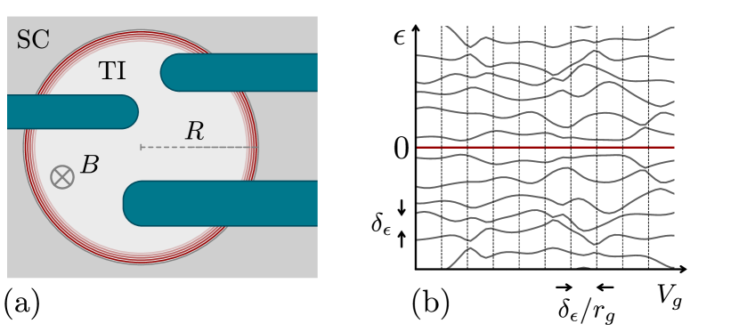
Statistical spectroscopy principles.—We propose a protocol where an effectively averaged spectral density is obtained by variation of external control parameters. To understand the principle, we note that if integrability is broken by impurities and/or asymmetric system boundaries, the variation of any system parameter will result in new realizations of the chaotic scattering potential Goldberg et al. (1991). Similar approaches have previously been applied in semiconductor devices Zumbühl et al. (2002) and nanowires Contamin et al. (2022) for generating effective ensemble averages of the tunneling conductance. As concrete example, we here formulate the approach for a TI vortex, cf. Fig. 1(a): An -wave superconductor is deposited on a TI surface except for a circular region of radius . Through this region an integer number, , of superconducting flux quanta is threaded ( throughout). For odd parity of , this synthetic vortex binds a zero energy MBS Hasan and Kane (2010).
Variations in the voltage of nearby finger gates, , parametrically change the system Hamiltonian. Even in the absence of “intrinsic” disorder, they break integrability and realize an effective ensemble average, provided the perturbation is strong enough to effectively scramble the spectrum of vortex states, cf. Fig.1(b). To estimate the required voltage variations, we make the conservative assumption that the Coulomb interaction across the vortex is strongly screened, and that only local wave functions right under the geometric finger gate surface are susceptible to the perturbation. To first order in perturbation theory, this leads to the estimate for the distortion of the energy, , of individual states. Here, the integral extends over the area underneath the gate, we assume approximate statistical uniformity of the wave function modulus, and is the fraction of the gate area relative to that of the vortex. Variations strong enough that the perturbation exceeds the level spacing, , effectively define a new realization of the spectrum, cf. Fig.1(b).
Provided the broadening, , of Andreev states due to disorder exceeds the level spacing , we expect level repulsion, and in the consequence the emergence of the spectral density in Eq. (1) upon averaging over an ensemble. Presently, this ensemble average is realized by sampling a large number of configurations distinguished by changes , and subsequently collecting the results in a histogram.
In a concrete experiment where each level spacing is divided into bins and the number of runs is , an average number of levels will be counted per bin. This number is subject to statistical fluctuations . To obtain a reliable result, the relative fluctuation must be smaller than the relative change , computed according to Eq. (1). A straightforward estimate for, say, leads to the conclusion that runs are required to obtain statistical certainty.
TI vortex.—In the following, we test the statistical protocol for the TI vortex setup in Fig. 1(a). The single-particle Bogoliubov-de Gennes Hamiltonian describing the proximitized TI surface is given by Hasan and Kane (2010)
| (2) |
where is the surface-state velocity, the chemical potential, and Pauli matrices () act in particle-hole (spin) space. In the London gauge, the pair potential is , with polar coordinates relative to the vortex center and assumed as step function like. The Hamiltonian (2) satisfies particle-hole symmetry, with and complex conjugation, placing it into symmetry class D. (For completeness, we mention that in the field free case, , we also have time reversal symmetry, with , implying an upgrade to class DIII.)
We add disorder to the vortex core in the form of a Gaussian correlated random potential with zero mean and variance . The corresponding scattering mean free path computed in Born approximation is given by sup . Comparison with the bound-state spacing of the clean vortex, , shows that the threshold to strong disorder mixing, , is reached when , i.e., when the quasi-particle motion crosses over from ballistic to diffusive. For stronger disorder, the characteristic level spacing shrinks to , i.e., from the inverse of the ballistic time of flight, , to the inverse of the diffusion time across the vortex, , see the SM sup for details.
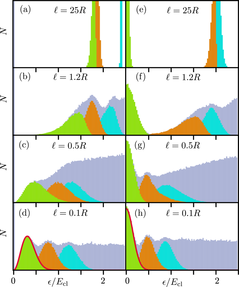
Our statistical approach to MBS spectroscopy works for disorder beyond the ballistic/diffusive threshold. To illustrate this point, Fig. 2 shows data histograms obtained from disorder realizations and for disorder strengths ranging from an almost perfectly ballistic regime, , to a diffusive one with . The columns on the left (right) are for a vortex with (without) MBS, realized here by setting (). In the ballistic regime, we observe weakly broadened states with spacings varying strongly at scales . Upon crossing into the diffusive regime, they start to overlap, along with a tendency towards a more uniform spacing — the level crystallization symptomatic for quantum chaotic spectra.
Real experiments have access to the cumulative contribution of all levels, here indicated in grey, where we observe the gradual approach to the profile in Eq. (1), as well as to the distribution of individual levels, cf. the green/orange/cyan histograms for the lowest three positive energy levels. For disorder deep in the diffusive regime, we expect the statistics of these levels to be described by the principles of random matrix theory Mehta (2004); Beenakker (2015). Specifically, for class D one expects the probability distribution for the lowest lying level in the case with [without] MBS to be given by Altland and Zirnbauer (1997); Beenakker (2015); sup . Figure 2 shows that these distributions, indicated as red curves, are clearly realized by the disordered vortex in the strong disorder regime. However, the most important conclusion is that the presence or absence of a MBS is clearly resolved via the statistics of the cumulative histogram, provided the focus of attention is shifted to the side bands, and the disorder is sufficient to induce inter-level correlations.
Experimental reality.—The analysis above assumed arbitrary energy resolution, and averaging over a large number of realizations. What happens under less ideal conditions? In an experiment, the potential describing impurities or scattering off device irregularities is fixed and different realizations of the spectrum are generated by variation of externally adjustable parameters. In the TI vortex, the magnetic field strength is likewise fixed, which leaves gate electrodes as the next best choice for generating a parameter set. To generate samples required for bins per level spacing (see above estimate), one may need to work with finger gates and the resulting -dimensional parameter space. As the gate voltages are meant to mimic “disorder”, it is best to use an asymmetric geometric design as indicated in Fig. 1. Electrodes with large electrode-to-vortex area ratio, , will generate optimal sensitivity of energy levels, .
The simulations discussed in the following were performed for bins, requiring runs. We worked with electrodes sup , and varying each of their voltages over a range generated the parameter space for up to statistically independent samples 222If no independent information on the characteristic level spacing is available, the latter may be estimated by measuring the spacing between peaks in the averaged spectral density.. Finally, we account for the broadening of individual levels due to temperature or environmental coupling by introducing a Lorentzian line width, , with . Here, is required to resolve the oscillatory pattern of the target spectral density, i.e., our method requires the resolvability of individual states 333Another source of uncertainty is due to the fact that tunnel spectroscopy measures point conductance, i.e., a quantity proportional to the product of spectral density and wave function moduli, where the latter remain unknown. However, one may expect that in a large data set, these variations efficiently average out..
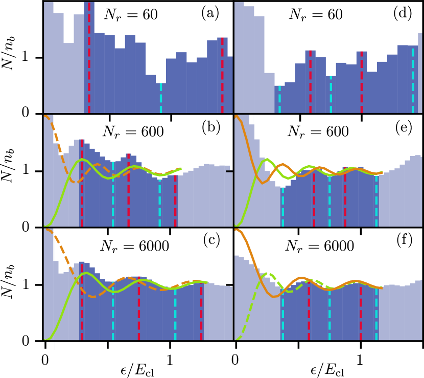
Given this setup, the minimal goal is a statistically sound distinction between the cases in Eq. (1). Figure 3 illustrates how the two cases are distinguished through a phase shift in the oscillatory spectral density at finite energy. In either case, a midgap peak is present (caused by a broadened MBS for , or a statistical accumulation of Andreev states for ). While these two peaks are difficult to distinguish, our method focuses on the spectrum away from the center. We note that in either case, the average spectral density contains a sequence of extrema at . The difference is that this sequence starts with a maximum (for ) or a minimum (for ). A more refined signature is obtained by subtracting a constant background and fitting the remaining oscillatory signal for the first, say, five extrema to Eq. (1), using as single fit parameter.
Fig. 3 shows data processed in this way for increasing number of runs , either with (left column) and without (right) MBS. The quality of the data may be assessed, e.g., by calculating the sum of squared distances between the extrema of the fit function and the data. For too low sample number, e.g., for , no unambiguous pattern of extrema is identifiable. At samples, side lobes begin to emerge, but a reliable assignment of extrema is still difficult to ascertain. However, for , the extremal energies are evenly spaced, and the squared distance fit accurately determines the correct sign of . Additional information on system parameters, such as knowledge of the effective broadening , may be exploited to develop more informed fitting protocols for the ensemble averaged data. However, we found that such refinements lead only to minor improvements of the results.
Let us briefly comment on the experimental feasibility of the TI vortex setup. Generally speaking the vortex area should be chosen small enough that its quantized levels can be resolved, and large enough that neighboring levels are coupled by disorder and gate variations. With , and given typical values m/s, nm Taskin et al. (2011), with spectral resolution eV, one needs to have m. Choosing nm and finger gates of width nm, we have . For these values, individual levels can be distinguished and a few finger gate electrodes could be placed over the vortex core. We are thus confident that the requirements for our proposal to work are met by existing setups.
Conclusions.—We have proposed a novel scheme for the detection of MBS in existing device structures which combines tunnel spectroscopy with elements of statistics. The focus of attention is here shifted from the center peak ubiquitous in spectroscopic data — which is notorious for its misinterpretability — to the pattern of side bands. The unavoidable presence of effective disorder becomes a resource in that it induces correlations between levels which, upon averaging over different parametric realizations, lead to the effectively crystalline structure in Eq. (1). The latter originates in a combination of statistics and topology which is unambiguously linked to the presence or absence of a MBS, even if the latter cannot be clearly identified in isolation. Another advantage of the approach is that it includes its own validation: If neither the positive, , nor the negative, , signal can be resolved, the method has not been implemented with sufficient accuracy. The principal conditions for it to work are resolvability of individual levels (where one may argue that this condition must be met anyway for the MBS to become a useful resource), sufficient statistics provided by at least runs, and effective disorder strong enough to cause level correlation. (If the “native” disorder is too weak, one may contemplate lowering the level spacing by increasing the vortex size for diagnostic purposes.) These criteria are realistic for the vortex platform, and we are confident that the same holds for other realizations, such as planar Josephson junctions, leaving sufficient freedom for the placement of gate electrodes. We conclude that this approach has the potential to settle the issue of MBS existence with available measurement protocols and hardware.
Acknowledgements.
We thank Y. Ando, C. Marcus, J. Schluck, and S. Vaitiekenas for discussions. We acknowledge funding by the Deutsche Forschungsgemeinschaft (DFG, German Research Foundation), Projektnummer 277101999 – TRR 183 (AA and RE, projects A01, A03, B04, and C01), under project No. EG 96/13-1, and under Germany’s Excellence Strategy – Cluster of Excellence Matter and Light for Quantum Computing (ML4Q) EXC 2004/1 – 390534769.References
- Alicea (2012) J. Alicea, Rep. Prog. Phys. 75, 076501 (2012).
- Leijnse and Flensberg (2012) M. Leijnse and K. Flensberg, Semiconductor Science and Technology 27, 124003 (2012).
- Beenakker (2013) C. W. J. Beenakker, Annual Review of Condensed Matter Physics 4, 113 (2013).
- DasSarma, Freedman, and Nayak (2015) S. DasSarma, M. Freedman, and C. Nayak, njp Quantum Inf. 1, 51001 (2015).
- Mourik et al. (2012) V. Mourik, K. Zuo, S. M. Frolov, S. R. Plissard, E. P. A. M. Bakkers, and L. P. Kouwenhoven, Science 336, 1003 (2012).
- Nadj-Perge et al. (2014) S. Nadj-Perge, I. K. Drozdov, J. Li, H. Chen, S. Jeon, J. Seo, A. H. MacDonald, B. A. Bernevig, and A. Yazdani, Science 346, 602 (2014).
- Lutchyn et al. (2018) R. M. Lutchyn, E. P. A. M. Bakkers, L. P. Kouwenhoven, P. Krogstrup, C. M. Marcus, and Y. Oreg, Nat. Rev. Mat. 3, 52 (2018).
- Liu et al. (2018) Q. Liu, C. Chen, T. Zhang, R. Peng, Y.-J. Yan, C.-H.-P. Wen, X. Lou, Y.-L. Huang, J.-P. Tian, X.-L. Dong, G.-W. Wang, W.-C. Bao, Q.-H. Wang, Z.-P. Yin, Z.-X. Zhao, and D.-L. Feng, Phys. Rev. X 8, 041056 (2018).
- Li et al. (2022) M. Li, G. Li, L. Cao, X. Zhou, X. Wang, C. Jin, C.-K. Chiu, S. J. Pennycook, Z. Wang, and H.-J. Gao, Nature 606, 890 (2022).
- MicrosoftQuantum (2022) MicrosoftQuantum, “Inas-al hybrid devices passing the topological gap protocol,” (2022), arXiv:2207.02472.
- Sengupta et al. (2001) K. Sengupta, I. Žutić, H.-J. Kwon, V. M. Yakovenko, and S. Das Sarma, Phys. Rev. B 63, 144531 (2001).
- Law, Lee, and Ng (2009) K. T. Law, P. A. Lee, and T. K. Ng, Phys. Rev. Lett. 103, 237001 (2009).
- Flensberg (2010) K. Flensberg, Phys. Rev. B 82, 180516 (2010).
- Sun et al. (2016) H.-H. Sun, K.-W. Zhang, L.-H. Hu, C. Li, G.-Y. Wang, H.-Y. Ma, Z.-A. Xu, C.-L. Gao, D.-D. Guan, Y.-Y. Li, C. Liu, D. Qian, Y. Zhou, L. Fu, S.-C. Li, F.-C. Zhang, and J.-F. Jia, Phys. Rev. Lett. 116, 257003 (2016).
- Zazunov, Egger, and Levy Yeyati (2016) A. Zazunov, R. Egger, and A. Levy Yeyati, Phys. Rev. B 94, 014502 (2016).
- Bolech and Demler (2007) C. J. Bolech and E. Demler, Phys. Rev. Lett. 98, 237002 (2007).
- Nilsson, Akhmerov, and Beenakker (2008) J. Nilsson, A. R. Akhmerov, and C. W. J. Beenakker, Phys. Rev. Lett. 101, 120403 (2008).
- Golub and Horovitz (2011) A. Golub and B. Horovitz, Phys. Rev. B 83, 153415 (2011).
- Haim et al. (2015) A. Haim, E. Berg, F. von Oppen, and Y. Oreg, Phys. Rev. Lett. 114, 166406 (2015).
- Liu, Cheng, and Lutchyn (2015) D. E. Liu, M. Cheng, and R. M. Lutchyn, Phys. Rev. B 91, 081405 (2015).
- Tripathi, Das, and Rao (2016) K. M. Tripathi, S. Das, and S. Rao, Phys. Rev. Lett. 116, 166401 (2016).
- Jonckheere et al. (2017) T. Jonckheere, J. Rech, A. Zazunov, R. Egger, and T. Martin, Phys. Rev. B 95, 054514 (2017).
- Jonckheere et al. (2019) T. Jonckheere, J. Rech, A. Zazunov, R. Egger, A. L. Yeyati, and T. Martin, Phys. Rev. Lett. 122, 097003 (2019).
- Manousakis et al. (2020) J. Manousakis, C. Wille, A. Altland, R. Egger, K. Flensberg, and F. Hassler, Phys. Rev. Lett. 124, 096801 (2020).
- Aasen et al. (2016) D. Aasen, M. Hell, R. V. Mishmash, A. Higginbotham, J. Danon, M. Leijnse, T. S. Jespersen, J. A. Folk, C. M. Marcus, K. Flensberg, and J. Alicea, Phys. Rev. X 6, 031016 (2016).
- Beenakker (2020) C. W. J. Beenakker, SciPost Phys. Lect. Notes , 15 (2020).
- Flensberg, von Oppen, and Stern (2021) K. Flensberg, F. von Oppen, and A. Stern, Nat. Rev. Mat. 6, 944 (2021).
- Sbierski et al. (2022) B. Sbierski, M. Geier, A.-P. Li, M. Brahlek, R. G. Moore, and J. E. Moore, Phys. Rev. B 106, 035413 (2022).
- Altland and Zirnbauer (1997) A. Altland and M. R. Zirnbauer, Phys. Rev. B 55, 1142 (1997).
- Beenakker (2015) C. W. J. Beenakker, Rev. Mod. Phys. 87, 1037 (2015).
- Bagrets and Altland (2012) D. Bagrets and A. Altland, Phys. Rev. Lett. 109, 227005 (2012).
- Liu et al. (2012) J. Liu, A. C. Potter, K. T. Law, and P. A. Lee, Phys. Rev. Lett. 109, 267002 (2012).
- Aguado (2017) R. Aguado, Riv. Nuovo Cimento 40, 523 (2017).
- Moore, Stanescu, and Tewari (2018) C. Moore, T. D. Stanescu, and S. Tewari, Phys. Rev. B 97, 165302 (2018).
- Vuik et al. (2019) A. Vuik, B. Nijholt, A. R. Akhmerov, and M. Wimmer, SciPost Phys. 7, 061 (2019).
- Prada et al. (2020) E. Prada, P. San-Jose, M. W. A. de Moor, A. Geresdi, E. J. H. Lee, J. Klinovaja, D. Loss, J. Nygård, R. Aguado, and L. P. Kouwenhoven, Nat. Rev. Phys. 2, 225 (2020).
- Valentini et al. (2021) M. Valentini, F. Peñaranda, A. Hofmann, M. Brauns, R. Hauschild, P. Krogstrup, P. San-Jose, E. Prada, R. Aguado, and G. Katsaros, Science 373, 82 (2021).
- Yu et al. (2021) P. Yu, J. Chen, M. Gomenko, G. Badawy, E. P. A. M. Bakkers, K. Zuo, V. Mourik, and S. Frolov, Nat. Phys. 17, 482 (2021).
- Frolov and Mourik (2022) S. Frolov and V. Mourik, (2022), majorana fireside podcast, https://youtu.be/RnYghkDaHH0.
- Akhmerov (2022) A. R. Akhmerov, (2022), what can we learn from the reported discovery of Majorana states? Journal Club Condensed Matter, see https://doi.org./10.36471/JCCM_July_2022_01.
- Akhmerov et al. (2011) A. R. Akhmerov, J. P. Dahlhaus, F. Hassler, M. Wimmer, and C. W. J. Beenakker, Phys. Rev. Lett. 106, 057001 (2011).
- Wimmer et al. (2011) M. Wimmer, A. R. Akhmerov, J. P. Dahlhaus, and C. W. J. Beenakker, New Journal of Physics 13, 053016 (2011).
- Brouwer et al. (2011) P. W. Brouwer, M. Duckheim, A. Romito, and F. von Oppen, Phys. Rev. Lett. 107, 196804 (2011).
- Neven, Bagrets, and Altland (2013) P. Neven, D. Bagrets, and A. Altland, New Journal of Physics 15, 055019 (2013).
- Diez et al. (2014) M. Diez, I. C. Fulga, D. I. Pikulin, J. Tworzydło, and C. W. J. Beenakker, New Journal of Physics 16, 063049 (2014).
- Haim and Stern (2019) A. Haim and A. Stern, Phys. Rev. Lett. 122, 126801 (2019).
- Mehta (2004) M. L. Mehta, Random Matrices (Academic Press, 2004).
- Fu and Kane (2008) L. Fu and C. L. Kane, Phys. Rev. Lett. 100, 096407 (2008).
- Hasan and Kane (2010) M. Z. Hasan and C. L. Kane, Rev. Mod. Phys. 82, 3045 (2010).
- Ioselevich, Ostrovsky, and Feigel’man (2012) P. A. Ioselevich, P. M. Ostrovsky, and M. V. Feigel’man, Phys. Rev. B 86, 035441 (2012).
- Akzyanov et al. (2014) R. S. Akzyanov, A. V. Rozhkov, A. L. Rakhmanov, and F. Nori, Phys. Rev. B 89, 085409 (2014).
- Røising et al. (2019) H. S. Røising, R. Ilan, T. Meng, S. H. Simon, and F. Flicker, SciPost Phys. 6, 055 (2019).
- Ziesen and Hassler (2021) A. Ziesen and F. Hassler, Journal of Physics: Condensed Matter 33, 294001 (2021).
- de Mendonça et al. (2022) B. S. de Mendonça, A. L. R. Manesco, N. Sandler, and L. G. G. V. D. da Silva, “Can caroli-de gennes-matricon and majorana vortex states be distinguished in the presence of impurities?” (2022), arXiv:2204.05078.
- Caroli, De Gennes, and Matricon (1964) C. Caroli, P. De Gennes, and J. Matricon, Physics Letters 9, 307 (1964).
- (56) See the online Supplementary Material (SM), where we provide additional details on peak spacing distributions, on the mean free path, on our numerical simulations, and on other Majorana platforms.
- Lei et al. (2010) H. Lei, R. Hu, E. S. Choi, J. B. Warren, and C. Petrovic, Phys. Rev. B 81, 094518 (2010).
- Xu et al. (2016) G. Xu, B. Lian, P. Tang, X.-L. Qi, and S.-C. Zhang, Phys. Rev. Lett. 117, 047001 (2016).
- Wang et al. (2018) D. Wang, L. Kong, P. Fan, H. Chen, S. Zhu, W. Liu, L. Cao, Y. Sun, S. Du, J. Schneeloch, R. Zhong, G. Gu, L. Fu, H. Ding, and H.-J. Gao, Science 362, 333 (2018).
- Jiang, Dai, and Wang (2019) K. Jiang, X. Dai, and Z. Wang, Phys. Rev. X 9, 011033 (2019).
- Machida et al. (2019) T. Machida, Y. Sun, S. Pyon, S. Takeda, Y. Kohsaka, T. Hanaguri, T. Sasagawa, and T. Tamegai, Nature Materials 18, 811 (2019).
- Kong et al. (2019) L. Kong, S. Zhu, M. Papaj, H. Chen, L. Cao, H. Isobe, Y. Xing, W. Liu, D. Wang, P. Fan, et al., Nature Physics 15, 1181 (2019).
- Zhang et al. (2018) P. Zhang, K. Yaji, T. Hashimoto, Y. Ota, T. Kondo, K. Okazaki, Z. Wang, J. Wen, G. D. Gu, H. Ding, and S. Shin, Science 360, 182 (2018).
- Zhu et al. (2020) S. Zhu, L. Kong, L. Cao, H. Chen, M. Papaj, S. Du, Y. Xing, W. Liu, D. Wang, C. Shen, F. Yang, J. Schneeloch, R. Zhong, G. Gu, L. Fu, Y.-Y. Zhang, H. Ding, and H.-J. Gao, Science 367, 189 (2020).
- Hell, Leijnse, and Flensberg (2017) M. Hell, M. Leijnse, and K. Flensberg, Phys. Rev. Lett. 118, 107701 (2017).
- Pientka et al. (2017) F. Pientka, A. Keselman, E. Berg, A. Yacoby, A. Stern, and B. I. Halperin, Phys. Rev. X 7, 021032 (2017).
- Fornieri et al. (2019) A. Fornieri, A. M. Whiticar, F. Setiawan, E. Portolés, A. C. C. Drachmann, A. Keselman, S. Gronin, C. Thomas, T. Wang, R. Kallaher, G. C. Gardner, E. Berg, M. J. Manfra, A. Stern, C. M. Marcus, and F. Nichele, Nature 569, 89 (2019).
- Ren et al. (2019) H. Ren, F. Pientka, S. Hart, A. T. Pierce, M. Kosowsky, L. Lunczer, R. Schlereth, B. Scharf, E. M. Hankiewicz, L. W. Molenkamp, B. I. Halperin, and A. Yacoby, Nature 569, 93 (2019).
- Marra (2022) P. Marra, Journal of Applied Physics 132, 231101 (2022).
- Goldberg et al. (1991) J. Goldberg, U. Smilansky, M. V. Berry, W. Schweizer, G. Wunner, and G. Zeller, Nonlinearity 4, 1 (1991).
- Zumbühl et al. (2002) D. M. Zumbühl, J. B. Miller, C. M. Marcus, K. Campman, and A. C. Gossard, Phys. Rev. Lett. 89, 276803 (2002).
- Contamin et al. (2022) L. C. Contamin, L. Jarjat, W. Legrand, A. Cottet, T. Kontos, and M. R. Delbecq, Nature Communications 13, 6188 (2022).
- Taskin et al. (2011) A. A. Taskin, Z. Ren, S. Sasaki, K. Segawa, and Y. Ando, Phys. Rev. Lett. 107, 016801 (2011).