Flow: Per-instance Personalized Federated Learning

Abstract

Federated learning (FL) suffers from data heterogeneity, where the diverse data distributions across clients make it challenging to train a single global model effectively. Existing personalization approaches aim to address the data heterogeneity issue by creating a personalized model for each client from the global model that fits their local data distribution. However, these personalized models may achieve lower accuracy than the global model in some clients, resulting in limited performance improvement compared to that without personalization. To overcome this limitation, we propose a per-instance personalization FL algorithm Flow. Flow creates dynamic personalized models that are adaptive not only to each client’s data distributions but also to each client’s data instances. The personalized model allows each instance to dynamically determine whether it prefers the local parameters or its global counterpart to make correct predictions, thereby improving clients’ accuracy. We provide theoretical analysis on the convergence of Flow and empirically demonstrate the superiority of Flow in improving clients’ accuracy compared to state-of-the-art personalization approaches on both vision and language-based tasks. The source code is available on GitHub .

1 Introduction

Federated Learning (FL) is a distributed machine learning paradigm that enables edge devices, known as “clients”, which collaboratively train a machine learning model called a “global model” [1]. However, because the server, which is the FL training orchestrator, does not have access to or knowledge of client data distributions, it poses a challenge of statistical heterogeneity [2, 3]. This heterogeneity hinders the server’s ability to train an ML model on a large quantity and variety of data and also impacts the client’s ability to benefit from a generalizable model without sharing any information about its data. To address this challenge, personalization has been studied [4, 5] to improve prediction performance. Recent literature consistently demonstrates that personalized models achieve higher prediction performance than the global model aggregated over clients [5, 6, 7, 8, 9, 10]. These approaches typically create a personalized model specific to each client’s data distribution, and thus we refer to them as “per-client personalization”.

However, we have identified two factors that limit the performance improvement of existing per-client personalization approaches in terms of clients’ accuracy. First, as reported in the evaluation in Sec. 5, we found that personalized models can achieve lower accuracy than the global model on up to 31% clients, causing limited improvement in accuracy averaged across all clients. Second, even if personalized models achieve higher accuracy on a client compared to the global model, they can still produce incorrect predictions on up to 11% of data instances on clients that could be correctly handled by the global model, causing limited accuracy improvement from personalization on that client. These observations reveal a significant drawback of existing per-client personalization approaches: each client’s personalized model is a static network that cannot accommodate the heterogeneity of the local client’s data instances. As a result, every data instance on a client is constrained to use its personalized model for prediction, even though some instances could benefit from the better generalizability of the global model.

To overcome the above limitation, this paper proposes a per-instance and per-client personalized FL algorithm Flow via dynamic routing to improve clients’ accuracy. Flow creates dynamic personalized models that are adaptive to each client’s individual data instances (per-instance) as well as their data distribution (per-client). In a FL round of Flow, each client has both the global model parameters that are shared across clients and the local model parameters that are adapted to the local data distribution of the client by fine-tuning the global model parameters. Flow creates a dynamic personalized model per client that consists of local and global model components and a dynamic routing module. The dynamic routing module allows each data instance on a client to determine whether it prefers the local model parameters or their global model counterparts to make correct predictions, thereby improving the personalized model’s accuracy on the client compared to that of a local model or a global model. At the same time, through dynamic routing, Flow could identify instances in each client that agree with the global data distribution to further improve the performance of the global model, offering a good starting point for any new client to personalize from. Since Flow is a client-side personalization approach, it can work with server-side optimization methods like FedYogi [11].

We theoretically analyze how dynamic routing affects the convergence of the global model and personalized model in Flow and also empirically demonstrate the effectiveness of Flow in improving clients’ accuracy compared to state-of-the-art personalization approaches on cross-device language and vision tasks. For the newly joined clients, the global model from Flow achieves 2.81% (Stackoverflow), 3.46% (Shakespeare), and 0.95%-1.41% (CIFAR10) better accuracy on the global model against its best performing baselines respectively. After personalization, the dynamic personalized model from Flow sees improvements of 3.79% (Stackoverflow), 2.25% (Shakespeare), and 3.28%-4.58% (CIFAR10) against the best performing baselines. Our in-depth analysis shows that Flow achieves the highest percentage of clients who benefit from personalization compared to all baselines and reduces the number of instances that are misclassified by the personalized model but correctly classified by the global model, contributing to the better personalized accuracy from Flow.

We summarize the contributions as follows:

• We propose a per-instance and per-client personalization approach Flow that creates personalized models via dynamic routing, which improves both the performance of the personalized model and the generalizability of the global model.

• We derive convergence analysis for both global and personalized models, showing how the routing policy influences convergence rates based on the across- and within- client heterogeneity.

• We empirically evaluate the superiority of Flow in both generalization and personalized accuracy on various vision and language tasks in cross-device FL settings.

2 Related Work

Personalized Federated Learning. Personalization in FL has been explored primarily on client-level granularity. APFL [6] interpolates client-specific local model weights with the global model weights which are sent by the server. Meanwhile, Flow is an intermediate-output interpolation method and also includes a dynamic policy to interpolate at instance-level granularity. We note that Dapper [12] interpolates the client dataset with a global dataset, which is impractical for the cross-device use cases FL focused on in this paper. Regularization is another popular way of creating a personalized model. It encourages a personalized model of each client to be close to the global model as explored in Ditto [13] and pFedMe [14]. Finetuning partial or entire global model to get the personalized model has been studied in LGFedAvg [7], which finetunes and personalizes the feature extractor and globally shares the classifier head, FedBabu [15] which freezes the classifier head and only updates and aggregates the feature extractor, and FedRep [8] which finetunes and personalizes the classifier head and globally shares the feature extractor. Learning personalized representations of the global model has been explored in FedHN [16] where a central hypernetwork model is trained to generate a personalized model for each client. PartialFed [17] makes a layer-wise choice between global and local models to create a personalized model, but it sends the personalized models back to the server in lieu of a separate global model. This method has limitations in terms of training the base global model (on which the personalized model would be based) with FedAvg, which has been observed to be insufficient against non-iid data [18]. Besides, the strategy does not create a dynamic personalized model during inference. None of the above work has explored instance-level personalization.

Personalized models from previous work knnPer [19] exhibits per-instance personalization behavior. The personalized model of a client makes a prediction based on features extracted from the global model from an instance as well as features from the instance’s nearest neighbors. However, knnPer trains the global model parameters in the same way as FedAvg, which has been shown to perform poorly in heterogeneous data settings [18]. In contrast, Flow’s dynamic routing mechanism results in a global model with better-generalized performance amidst heterogeneous instances, which ultimately leads to a higher boost in the performance of personalized models as well.

Dynamic Routing. Motivated by saving compute effort for “easy to predict” instances, instance-level dynamic routing has been a matter of discussion in works related to early exiting [20, 21, 22], layer skipping [23], and multi-branching [24, 25]. SkimRNN [26] explored temporal dynamic routing where depending on the input instance, a trained policy can determine whether to skim through the instance with a smaller RNN layer (which just updates the hidden states partially), or read the instance with a standard (bigger) RNN layer (updating the entire hidden state). Our work is motivated by the question of Depending on the models’ utility and instances’ heterogeneity, which route to pick?. This can be achieved by using a routing policy to dynamically pick from two versions of a model, which are equivalent in terms of computational cost but different in terms of the data they are trained on.

3 Our Approach

We introduce Flow, a per-instance and per-client personalization method that dynamically determines when to use a client’s local parameters and when to use the global parameters based on the input instance. Table 1 summarizes the notation used in this paper.

Table 1: Notations

$K$	#Epochs for training
$M$	Total number of sampled clients
$m$	Client index $\in[M]$
$\mathcal{M}{}$	Set of available clients
$p$	Client sampling rate
$\eta_{\ell}$	Local learning rate
$w_{g}$	Global model
$\psi_{g}$	Policy module
$w_{g,m}{}$	Local version of the global model
$w_{\ell,m}{}$	Local model of $m^{th}$ client
$w_{p,m}{}$	Personalized model of $m^{th}$ client
$\mathcal{D}_{m}$	Data distribution of $m^{th}$ client

Algorithm 1 describes the workflow of Flow. During each FL round, the server samples $M$ participating clients with a sampling rate of $p$. Upon receiving the global model $w_{g}$ and policy parameters $\psi_{g}$ (Line 1), each participating client personalizes and trains $w_{g}$ in five major stages: (1) Split the training dataset into two halves: $\zeta_{m,\ell}$ and $\zeta_{m,g}$ (Line 1). $\zeta_{m,\ell}$ will be used to update the parameters in the local model parameters while $\zeta_{m,g}$ will be used to train the parameters in the global model and a routing module. (2) Derive the local parameters $w_{\ell}$ by finetuning the global parameters $w_{g}$ for $K_{1}$ epochs with $\zeta_{m,\ell}$ (Line 1). (3) Construct a dynamic personalized model $w_{p,m}$ by integrating the local versions of the global parameters $w_{g,m}$ and policy parameters $\psi_{g,m}{}$, and the local parameters $w_{\ell}$. Here, the routing policy $\psi_{g}$ determines whether the execution path of an instance should use $w_{\ell}$ or $w_{g}$. (4) Train the routing policy $\psi_{g,m}{}$ and the local version of the global parameters $w_{g,m}{}$ alternatively for $K_{2}$ epochs (Lines 1-1) with $\zeta_{m,g}$. Although $K_{1}$ and $K_{2}$ can be different, we later use $K$ to denote both $K_{1}$ and $K_{2}$ for ease of theoretical analysis. (5) Send the local version of the global model parameters $w_{g,m}{}$ and the policy parameters $\psi_{g,m}{}$ back to the server for aggregation (Line 1). Aggregation strategies are orthogonal to this work and we adopt FedAvg [1].

Next, we discuss the design of the dynamic personalized model $w_{p}$ in detail. Figure 1 illustrates the design of $w_{p}$. In Flow, $w_{p}$ is made of three components, the local model $w_{\ell}$ and global model $w_{g}$ and the routing module $\psi_{g}$ that selects the execution of local or global model layers for each data instance.

Local Parameters.

We use finetuning to get the local parameters $w^{(r)}_{\ell,m}$ in the $r$-th round since finetuning has proven to be a less complex yet very effective method of personalization [27, 28]. Given a global model of the previous round, $w^{(r)}_{g,m}$, we finetune it for $K$ epochs to get $w^{(r)}_{\ell,m}$. This local model would be reflective of the client’s data distribution $\mathcal{D}_{m}$. Note that we use one half of the dataset to get $w^{(r)}_{\ell,m}$ and reserve the other half of the training dataset for updating the global model and the policy (i.e., the routing module) parameters. This is to make sure that the policy parameters, which would decide between local and global layers based on each input instance, are not overfitted in favor of the local parameters. In Figure 1, the local parameters are shaded green, denoted by $w_{\ell}$. The update rule for $w^{(r)}_{\ell,m}$ is:

$$w^{(r,K)}_{\ell,m}\leftarrow w^{(r,0)}_{\ell,m}-\eta_{\ell}\sum_{k=1}^{K}\nabla f_{m}(w^{(r,0)}_{\ell,m};\zeta_{m,\ell}),\text{ where }w^{(r,0)}_{\ell,m}:=w^{(r)}_{g}.$$ (1)

1 Server randomly initializes the global model $w_{g}$ and the policy module $\psi_{g}$ 2 for each round do 3       Send $w_{g}$, $\psi_{g}$ to sampled $M$ clients 4       5      for $m\in[M]$ in parallel do 6             $w_{g,m}{}\leftarrow w_{g}$; $\psi_{g,m}{}\leftarrow\psi_{g}$; $w_{\ell,m}{}\leftarrow w_{g,m}{}$ 7             Creating two mutually exclusive datasets $\zeta_{m,\ell},\zeta_{m,g}\leftarrow\mathcal{D}_{m}$ 8             Train $w_{\ell,m}{}$ for $K_{1}$ epochs 9             for $k\in[K_{2}]$ epochs do 10                   Update $\psi_{g,m}{}$ according to Equation 4 11                   Update $w_{g,m}{}$ according to Equation 5 12             end for 13            Send back $w_{g,m}{}$, $\psi_{g,m}{}$, $n_{m}$ := $|\zeta_{m,g}|$ 14       end for 15      Update $w_{g}$ and $\psi_{g}$ with weighted average of each client’s $w_{g,m}{}$ and $\psi_{g,m}{}$ 16       17 end for Algorithm 1 Pseudocode of Flow

Figure 1: Illustration of the dynamic personalized model design proposed by Flow.

Routing Module.

The routing module is a model with fully connected layers, shown as $\psi_{\text{base}}$ in Figure 1. After each layer $\psi_{\text{base}}$, the model has early exits denoted as $\psi_{\text{exit}}$ which outputs a probability of choosing the layer in the global model $w_{g}$ or the local model $w_{\ell}$. This probability at layer $j\in[L]$ is computed as,

$$\mathbf{q}^{(j)}=[\mathbf{q}^{(j)}_{0},\mathbf{q}^{(j)}_{1}]=\text{softmax}(\psi^{(j)}_{\text{exit}}(\psi^{(j)}_{\text{base}}(\hat{x})))\in[0,1]^{2}\text{ where }\begin{cases}\hat{x}\leftarrow x_{m}\quad\text{if $j=0;$}\\ \hat{x}\leftarrow\psi^{(j-1)}_{\text{base}}(\cdot)\text{ otherwise,}\end{cases}$$ (2)

where $\mathbf{q}^{(j)}_{0}$ and $\mathbf{q}^{(j)}_{1}$ are the probability of picking the global parameter $w^{(j)}_{g,m}$ and the local parameter $w^{(j)}_{\ell,m}$ respectively.

In order to train the routing parameters, we compute the training loss based on the output of the personalized model $w^{(r)}_{p,m}$, which averages the global model’s output and local model’s output weighted by $\mathbf{q}^{(j)}$, for each layer $j\in[L]$:

$$w^{(j)}_{p,m}(\hat{x})\leftarrow\mathbf{q}^{(j)}_{0}\cdot w^{(j)}_{g,m}(\hat{x})+\mathbf{q}^{(j)}_{1}\cdot w^{(j)}_{\ell,m}(\hat{x})\text{ where }\begin{cases}\hat{x}\leftarrow x_{m}\quad\text{if $j=0$;}\\ \hat{x}\leftarrow w^{(j-1)}_{p,m}(\cdot)\quad\text{ otherwise.}\end{cases}$$ (3)

Let $f_{m}(\cdot)$ denote the loss function on client $m$. Using the above personalized model $w^{(r)}_{p,m}$, Flow updates the policy parameters as follows,

$$\psi^{(r+1)}_{g,m}\leftarrow\psi^{(r)}_{g,m}-\eta_{\ell}\nabla_{\psi^{(r)}_{g,m}}\left[f_{m}(w^{(r)}_{p,m};w_{g}^{(r)},\zeta_{m,g})-\frac{\gamma}{L}\sum_{j\in[L]}\log(\mathbf{q}^{(j)}_{0})\right],$$ (4)

where $-\frac{\gamma}{L}\sum_{j\in[L]}\log(\mathbf{q}^{(j)}_{0})$ is a regularization term that encourages the global model to learn on heterogeneous instances to improve the global model’s generalizability.

Global Parameters.

Global parameters $w_{g}$ are trained alternatively with the routing parameters $\psi_{g}$. Flow updates the global parameters as follows,

$$w^{(r+1)}_{g,m}\leftarrow w^{(r)}_{g,m}-\eta_{\ell}\nabla_{w^{(r)}_{g,m}}f_{m}(w^{(r)}_{p,m};\psi^{(r+1)}_{g,m},\zeta_{m,g})$$ (5)

The goal of the alternative training is for the instances that are characterized better by the global data distribution to get diverted to the global model and the rest of the instances that are captured better by the local data distribution routed to the local model. This improves the stability of the global model compared to approaches like APFL or knnPer which still use the global model trained on all the instances, regardless of the level of heterogeneity. The effectiveness of the alternative training is validated empirically and discussed in Appendix D.2.

Soft versus Hard Policy.

During training, we use soft policy where the probability in Equation 2 ranges over $[0,1]$ to update the parameters in the global model and the routing module. But during inference, we use a discrete version of the policy round$(\mathbf{q}^{(j)})\in\{0,1\}^{2}$ for $\mathbf{q}^{(j)}$ in Eq. 3. The rationale behind this is twofold: (a) Using hard policy saves compute resources during inference by executing either the global or the local layer for an instance instead of both. (b) Our empirical evaluation shows negligible difference in performance of personalized models with soft and hard policies during the inference.

The dynamic nature of the personalized model in Flow introduces additional storage and computational overhead compared to the canonical method FedAvg with Fine Tuning (called FedAvgFT). However, compared to other state-of-the-art personalization methods such as Ditto and APFL, Flow requires similar or even less storage and computational overhead. Detailed analysis and comparison with baselines is in Appendix C.

4 Theoretical Analysis

In this section, we give convergence bounds for the global model $w_{g}$ and the personalized model $w_{p}$ of an arbitrary client $m$ in smooth non-convex cases. The bounds for strong and general convex cases are available in Appendix E, Sections E.3 and E.5. To derive the bounds, we adopt two commonly used assumptions in FL convergence analysis from AFO (Assumption 2, [11]) and SCAFFOLD (Assumption 1, [18]): (1) We assume local variance between a client’s expected and true gradient is $\sigma_{\ell}$-bounded. (2) We also assume that the dissimilarity between aggregated gradients of local expected risk and the true global gradient is $(G,B)$-bounded, where both $G$ and $B$ are constants capturing the extent of gradient dissimilarities. A detailed description is in Appendix Section E.2.

Now we present the bounds on the norm of expected global (and local) risks on global (and personalized) models respectively, at $R$-th (last) round. The proofs are in Appendix Sections E.3 and E.5.

Theorem 4.1 (Convergence of the Global Model).

If each client’s objective function $f_{m}$ (and hence the global objective function $F$) satisfies $\beta$-smoothness, $\sigma_{\ell}$-bounded local gradient variance, $(G,B)$-dissimilarity assumptions, using the learning rate $\frac{1}{2\beta}\leq\eta_{\ell}\leq\frac{1}{2\sqrt{5}\beta BK^{2}\sqrt{R}}$ [for non-convex case] in Flow, then the following convergence holds:

$$\frac{1}{R}\sum_{r=1}^{R}\mathbb{E}\left\|\nabla F(w^{(r)}_{g})\right\|^{2} \leq\frac{2}{\eta_{\ell}\mathbf{q}^{2}_{0}R}\left[\mathbb{E}\left[F(w^{(1)}_{g})\right]-\mathbb{E}\left[F(w^{(R+1)}_{g})\right]\right]$$

$$\qquad+\frac{\sigma_{\ell}^{2}}{2\sqrt{5}BM\mathbf{q}^{2}_{0}K\sqrt{R}}+\frac{2\mathbf{q}^{2}_{1}G^{2}}{\mathbf{q}^{2}_{0}B^{2}R}+\frac{\sigma_{\ell}^{2}}{B^{2}KR}.$$

Discussion.

Here, $\mathbf{q}_{0}^{2}$ (and $\mathbf{q}_{1}^{2}$) are the probability of picking the global (and local) weights averaged over all instances sampled from the global data distribution. Given a fixed $\mathbf{q}_{0}^{2}$ and $\mathbf{q}_{1}^{2}$, a larger $G$ increases the bound, indicating slower convergence of the global model due to higher heterogeneity. We made two additional observations on the convergence of Flow depending on $\mathbf{q}_{0}^{2}$ in the bound.

One the one hand, when $\mathbf{q}_{0}^{2}\rightarrow 1$, Flow matches the linear (strong convex) and sub-linear (general convex and non-convex) convergence rates of FedAvg [18]. Specifically, $\mathbf{q}_{0}^{2}=1$ results in convergence rate of $\mathcal{O}(1/R^{2})$ (strong convex), $\mathcal{O}(1/R^{2/3})$ (general convex), and $\mathcal{O}(1/R)$ (non-convex). When $\mathbf{q}_{0}^{2}=1$, which also indicates $\mathbf{q}_{1}^{2}=0$, the local parameters do not influence global model updates since all instances on a client will be routed to the global model and their gradients solely depend on the global model parameters. Flow degrades to FedAvg in this case in terms of the convergence of the global model.

On the other hand, when $\mathbf{q}_{0}^{2}\rightarrow 0$ indicating all instances are likely to be routed to the local model, the bound goes to infinity. It is because the global model parameters won’t get updated and thus won’t be able to converge. This observation validates the necessity of the regularization term in Eq. 4 to encourage instances to pick global model parameters.

Now we present the convergence bounds of the personalized model for the $m$-th client. The bound uses a definition of gradient diversity (noted as $\delta_{m}$) to quantify the diversity of a client’s gradient with respect to the global aggregated gradient, following the prior work [29]. Higher diversity implies higher heterogeneity of the client.

Theorem 4.2 (Convergence of the Personalized Model).

If each client’s objective function $f_{m}$ satisfies $\beta$-smoothness, $\sigma_{\ell}$-bounded local gradient variance, $(G,B)$-dissimilarity assumptions, and using the learning rate $\eta_{\ell}\leq\frac{1}{K\sqrt{12\beta R}}$ [for non-convex case] in Flow, then the following convergence holds:

$$\frac{1}{R}\sum_{r=1}^{R} \mathbb{E}||\nabla f_{m}(w^{(r,K)}_{p,m})||^{2}\leq\frac{2}{R}\left(\mathbb{E}\left[f_{m}(w^{(1,K)}_{p,m})\right]-\mathbb{E}\left[f_{m}(w^{(R,K)}_{p,m})\right]\right)$$

$$\qquad+\mathcal{O}\left(\frac{\beta^{2}}{R^{2}K^{2}}\left(\sigma_{\ell}^{2}+\left(\delta^{\psi_{g}}_{m}+\frac{\delta^{\psi_{g}}}{M}\right)K\right)\left(G^{2}+\frac{\mathbf{q}^{2}_{1,m}G^{2}}{\mathbf{q}^{2}_{0,m}R}\right)\right)$$

Discussion.

The theorem implies two main properties of the personalized models in Flow. First, for all convex and non-convex cases, the convergence rate of the personalized model in Flow is affected by the routing policy through the ratio ${\mathbf{q}^{2}_{1,m}}G^{2}/{\mathbf{q}^{2}_{0,m}}$. We know that a higher value of the gradient dissimilarity constant $G$, indicates higher heterogeneity between the aggregated and expected global model. The ratio of ${\mathbf{q}^{2}_{1,m}}/{\mathbf{q}^{2}_{0,m}}$ would be higher for a heterogeneous client, since the client would get a higher probability of picking the local route ($\mathbf{q}^{2}_{1,m}\rightarrow 1$). The higher $G$ and $\mathbf{q}^{2}_{1,m}$ results in slower convergence. On the contrary, a homogeneous client would benefit from a low value of ${\mathbf{q}^{2}_{1,m}}/{\mathbf{q}^{2}_{0,m}}$, which would offset the high value of $G$. Hence a homogeneous client’s personalized model would converge faster than the one of a heterogeneous client. Second, we observe that gradient diversity of the policy model, $\delta_{m}^{\psi_{g}}$, linearly affects the personalized model’s convergence. Since the policy model is also globally aggregated, a heterogeneous client would have a high $\delta_{m}^{\psi_{g}}$ and need more epochs per round to converge.

5 Experiments and Results

We empirically evaluate the performance of Flow against various personalization approaches for five non-iid vision and language tasks in terms of clients’ accuracy.

Datasets, Tasks, and Models. We have experiments on two language and three vision tasks. The first three datasets which are described below represent real-world heterogeneous data where each author or user is one client. (a) Stackoverflow [30] dataset is used for the next word prediction task, using a model with 1 LSTM and 2 subsequent fully connected layers. (b) Shakespeare [31] dataset is for the next character prediction task, using a 2 layer LSTM + 1 layer fully connected model. (c) EMNIST [32] dataset is for 62-class image classification, which uses 2 CNN layers followed by 2 fully-connected layers. The models for the above three datasets have been described in [11]. The next two datasets are federated and artificially heterogeneous versions of CIFAR10/100 datasets. (d-e) CIFAR10/100 [33] datasets are for 10- and 100-class image classification tasks with ResNet18 [34] model. Both CIFAR10/100 have two heterogeneous versions each: 0.1-Dirichlet is more heterogeneous, and 0.6-Dirichlet is less heterogeneous. Details about the datasets and the hyperparameters are in Appendix B.

Baselines and Metrics. We compare Flow with the following baselines: the classic FL algorithms FedAvg [35], state-of-the-art personalized FL approaches including FedAvgFT (FedAvg + Finetuning) [36], PartialFed [17], APFL [6], FedRep [8], LGFedAvg [7], Ditto [13], HypCluster [12], and knnPer [19], and the Local baseline which trains a local model on each client’s dataset without any collaboration. We use the adaptive version of PartialFed as it shows better performance compared to the alternatives in [17]. We evaluate Flow and these baselines in terms of generalized accuracy and personalized accuracy, which correspond to the accuracy of the global model and the personalized model on clients’ test data split.

We use Flower [37] library to implement Flow and all its baselines. We use an NVidia 2080ti GPU to run all the experiments with 3 runs for each. The random seeds used are 0, 44, and 56. We do not observe significant difference in results using other random seeds (see results in Appendix D.4).

5.1 Performance Comparison

Generalized and Personalized Accuracy. The performance of Flow and its baselines are reported in Table 2 for four datasets. Note that the local baseline has only personalized accuracy as it doesn’t create a global model collaboratively. The FedAvg has only generalized accuracy as it doesn’t personalize the global model for each client. Since PartialFed is a stateful approach, we are unable to run it on the cross-device datasets (Stackoverflow, Shakespeare, EMNIST). Results for the rest of the datasets and their variance across 3 different runs are reported in Appendix D.

Table 2: Generalized ($Acc_{g}$) and Personalized ($Acc_{p}$) accuracy (the higher, the better) for Flow and baselines.

Datasets	Stackoverflow		Shakespeare		CIFAR10 (0.1)		CIFAR10 (0.6)
Baselines	$Acc_{g}$	$Acc_{p}$	$Acc_{g}$	$Acc_{p}$	$Acc_{g}$	$Acc_{p}$	$Acc_{g}$	$Acc_{p}$
Local	-	15.93%	-	18.70%	-	49.78%	-	62.74%
FedAvg	23.15%	-	52.00%	-	60.98%	-	67.50%	-
FedAvgFT	23.83%	24.41%	52.12%	53.68%	61.23%	73.03%	68.19%	72.21%
knnPer	23.16%	24.49%	51.87%	53.10%	59.62%	75.14%	69.22%	70.14%
PartialFed	-	-	-	-	62.57%	73.20%	66.93%	70.38%
APFL	22.96%	25.70%	52.38%	53.64%	62.87%	72.86%	69.53%	72.53%
Ditto	22.59%	24.36%	52.44%	53.95%	62.06%	72.06%	68.12%	70.31%
FedRep	18.92%	21.04%	46.71%	50.09%	64.85%	68.62%	69.77%	63.61%
LGFedAvg	22.61%	24.03%	51.08%	51.43%	56.63%	73.19%	67.48%	68.94%
HypCluster	23.75%	22.43%	51.92%	52.74%	63.64%	71.55%	65.44%	72.40%
Flow (Ours)	26.64%	29.49%	55.90%	56.20%	66.26%	76.47%	70.88%	77.11%

Overall, Flow achieves 1.11-3.46% higher generalized accuracy and 1.33-4.58% higher personalized accuracy over the best performing baseline. In particular, Flow outperforms knnPer, another per-instance per-client personalization approach, by 1.66-6.64% and 1.33-6.97% in generalized and personalized accuracy metrics respectively. knnPer allows each instance to personalize the prediction of the global model based on its k-nearest neighbors at inference time. However, the global model is trained through the classic FL method FedAvg, which is agnostic to the heterogeneity of data instances. In contrast, Flow trains the global model differently via a parameterized dynamic routing module, which learns to put emphasis on data instances that are more aligned with the global data distribution to improve the performance of the global model.

Flow also outperforms the per-client personalization approaches including APFL, Ditto, HypCluster, and FedAvgFT by 1.35-3.46 % (generalized accuracy) and 2.25-4.58% (personalized accuracy).

Table 3: % of clients for which $Acc_{p}>Acc_{g}$ (the higher, the better).

	Stackoverflow	Shakespeare	CIFAR10 (0.1)	CIFAR10 (0.6)
FedAvgFT	79.26%	79.00%	97.18%	99.33%
knnPer	82.73%	68.87%	90.00%	90.00%
PartialFed	-	-	88.30%	84.80%
APFL	69.66%	79.22%	87.48%	90.63%
Ditto	74.59%	73.74%	90.52%	89.61%
FedRep	91.53%	79.78%	92.30%	84.64%
LGFedAvg	83.47%	88.43%	88.41%	89.59%
HypCluster	80.46%	74.84%	95.11%	98.18%
Flow (Ours)	92.74%	89.77%	98.33%	99.62%

We see improvements in generalized accuracy of Flow because of the fact that the global model in Flow is trained based on the instances which align more with the global distribution. We see improvements in personalized accuracy due to the limitation of the per-client approaches where some instances being correctly classified by the global model are incorrect on the personalized model. We next give insights on why Flow achieves better performance in personalized and generalized accuracy compared to these personalized baselines.

Percentage of Clients Benefiting from Personalization. The goal of personalization is to achieve higher prediction accuracy in each client by creating a per-client personalized model from the global model. We can thus measure the effectiveness of personalization by computing the percentage of clients for which the personalized model achieves higher task accuracy than the global model. The higher the percentage is, the better (or more effective) the personalization approach is.

Table 3 reports the results. We observed that Flow achieves the highest percentage of clients who benefit from personalization compared to all personalization baselines, echoing the better personalized accuracy from Flow. The percentage of clients who prefer personalized models can be as low as 68.87% (KnnPer on Shakespeare), which means personalization hurts up to 31% of clients’ accuracy, as mentioned in the introduction. As a contrast, Flow improves the percentage of clients benefiting from personalization to 89.77%-99.62% because each instance, in a client, has a choice between the global model parameters and the local model parameters and can choose the one that better fits it. Note that the comparison is in favor of the baselines since Flow also achieves better generalized accuracy, which makes it even harder for personalized models to further improve prediction accuracy.

Breakdown of Correctly Classified Instances. Figure 3 further shows the breakdown of the percentage of instances that are (a) correctly classified by the global model but not the personalized model (noted as global-only, colored in yellow ), (b) correctly classified by the personalized model but not the local model (noted as personalized-only, colored in blue ), and (c) correctly classified by both models (noted as both-correct, colored in green in Flow and baselines on Stackoverflow. The percentage of instances in y-axis is averaged over the test splits of all clients.

Overall, Flow increases the both-correct bars compared to all the baselines, which are the instances that contribute to the generalized performance of the global model. This explains the better generalized accuracy of Flow. Flow also increases the personalized-only bars and decreases the global-only bars, which correspond to the heterogeneous instances that prefer personalized models instead of the global model. This further explains the better personalized accuracy of Flow. Notably, for Stackoverflow dataset, existing personalization approaches still result in up to 4.74-7.93% of instances incorrectly classified by the personalized model but correctly by the global model. Flow reduces it to 1.12-2.42%. Similarly for the CIFAR10 (0.6) dataset, as mentioned in the introduction, we notice up to 11.4% of instances falling under the global-only category, which Flow reduces to 2.55%. It echoes the aforementioned effectiveness of personalization in Flow. The instance-wise accuracy breakdown for the rest of the datasets is detailed in Appendix D, Figure 10.

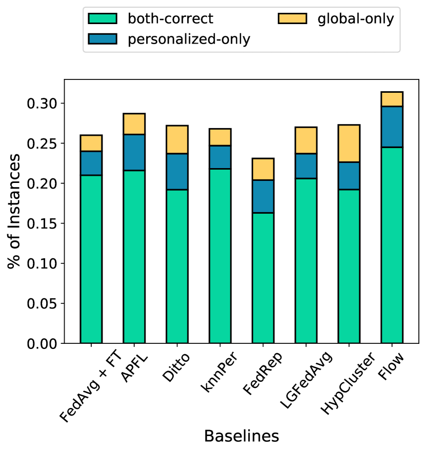
Figure 2: $w_{g}$ and $w_{p}$ accuracies for Stackoverflow.

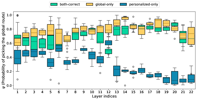
Figure 3: Behavior of the routing policy from $\psi_{g}$ for all instances at each layer for Stackoverflow.

Analysis of Routing Decisions. We further analyze the behavior of routing decisions for instances of a client that fall in the above three cases, global-only, personalized-only, and both-correct. Figure 3 shows the per-layer routing policies of the dynamic personalized model from Flow on Stackoverflow. For instances that fall into each category, we average the policy value from Eq. 2 and report the statistics on the probability of picking the global parameters for each layer. The statistics for the rest of the datasets are detailed in Appendix D.

For instances that are correctly classified by $w_{g}$ but not by $w_{p}$ (global-only), we see a clear trend of the routing parameters getting more confident about picking the global parameters. As a contrast, for instances that are correctly classified by $w_{p}$ but not by $w_{g}$ (personalized-only), we see the trend of routing policy being more confident in picking the local parameters. For instances that can be correctly classified by both models (both-correct), the routing policy still prefers the global parameters over local parameters. This is due to the regularization term in Eq. 4, which encourages instances to pick the global model over the local model in order to improve the generalizability of the global model. Our ablation study in the next section demonstrates the importance of regularization.

5.2 Ablation Studies

Here we highlight some results of three ablation studies on regularization, per-instance personalization, dynamic routing, and hard policies during inference. More results are in Appendix D.

(a) Ablation on the regularization term

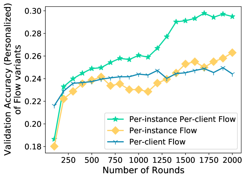
(b) Ablation on per-instance personalization design

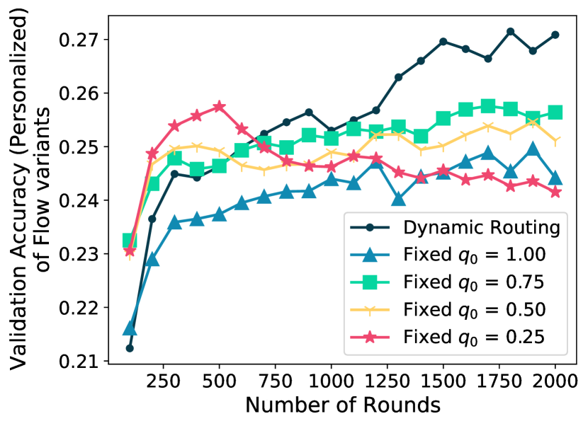
(c) Ablation on dynamic routing component

Figure 4: Ablation studies on Stackoverflow dataset.

Regularization. The regularization term in Eq. 4 promotes the global model layers whenever possible. It helps boost the generalized performance of the global model, which in turn also produces better personalized models. We use the results on the Stackoverflow dataset in Figure 4(a) to illustrate the importance of regularization. At the end of the training, we get 26.64% $\pm$ 0.23% generalized accuracy with regularization, compared to 24.16% $\pm$ 0.34% without regularization, and 29.49% $\pm$ 0.28% personalized accuracy with regularization, compared to 27.59% $\pm$ 0.36% without regularization. The importance of regularization in the policy update rule is also highlighted in Theorem 4.1, which states that only picking local route does not lead to global model convergence; the regularization term can encourage the global model to converge faster.

Per-instance Personalization. The dynamic personalized model in Flow allows each instance to choose between the local model and global model layers. To verify this per-instance personalization design, we create two variants of Flow, named “Per-Instance” Flow (pi-Flow) where both paths of a dynamic model are global models, and “Per-Client” Flow (pc-Flow) which is simply FedAvgFT. Compared to the personalized accuracy of per instance and per client Flow (29.49% $\pm$ 0.28%), pi-Flow and pc-Flow achieve $26.31\%\pm 0.19\%$ and $24.41\%\pm 0.26\%$ respectively on Stackoverflow dataset, as shown in Figure 4(b). The results demonstrate the effectiveness of the per-instance personalization design in Flow.

Dynamic Routing. This ablation study aims to learn whether dynamically interpolating global and local routes has any advantages over fixing the routing policy throughout the training. In Figure 4(c), we compare the validation accuracy curves of dynamic routing in Flow and dynamic routing with instance-agnostic static routing during the training phase. We observe that (a) For the case of fixed policy of $\mathbf{q}_{0}=0.25$, the validation accuracy has bad performance due to the fixed policy only choosing the local route. This is due to using hard policy during inference, and (b) The cases of fixed policy $\mathbf{q}_{0}\in[0.50,0.75,1.00]$ will only pick the global route during inference, which are also outperformed by the dynamic routing variant. With dynamic routing, the choice between local and global parameters depends on each instance during inference.

Soft versus Hard Decisions during Inference. We did not use soft decisions during inference since it only negligibly improves the accuracy of Flow. The test accuracies after personalization for Flow on Stackoverflow with hard decisions are 29.49% $\pm$ 0.28%, while with soft decisions, we observed 29.57% $\pm$ 0.22%. The rest of the datasets show a similar trend (see Appendix D, Table 8).

6 Conclusion

This paper proposed Flow, a per-instance and per-client personalization method to address the statistical heterogeneity issue in Federated Learning. Flow is motivated by the observation that the personalized models from existing personalized approaches achieve lower accuracy in a significant portion of clients compared to the global model. To overcome this limitation, Flow creates dynamic personalized models with a routing policy that allow instances on each client to choose between global and local parameters to improve clients’ accuracy. We derived error bounds for global and personalized models of Flow, showing how the routing policy affects the rate of convergence. The theoretical analysis validates our empirical observations related to clients preferring either a global or a local route based on the heterogeneity of individual instances. Extensive evaluation on both vision and language-based prediction tasks demonstrates the effectiveness of Flow in improving both the generalized and personalized accuracy.

Appendix A Limitations, Future Work, and Broader Impact

Learning on naturally heterogeneous datasets can be challenging, as the true data distributions of individual clients are unknown, making it difficult to correlate the divergence between client data distribution and the global data distribution with routing policy decisions. In our approach, we estimate the distribution divergence by measuring the difference between inference losses on global and local models, which helps us reason about routing probabilities for global and local routes. To further improve our understanding of the model performance, we plan to propose a metric that quantifies the difference in performance when a particular dataset is included versus excluded.

Flow has shown the promise of per-instance personalization in improving clients’ accuracy. This approach also holds the potential of preserving privacy by protecting against gradient leakage [38, 39, 40] and membership inference [41, 42] attacks that are easier to carry out in vanilla FL. Studying the relationship between personalization and privacy, and comparing our approach to traditional methods like Differential Privacy (DP) [43, 44] can reveal properties of personalization that go beyond improved accuracy.

Appendix B Datasets and Hyperparameters

Stackoverflow

The Stackoverflow dataset [30] is comprised of separate clients designated for training, validation, and testing. The dataset contains a total of 342,477 train clients, whose combined sample count equals 135,818,730. Similarly, the dataset contains 38,758 validation and 204,088 test clients, whose combined sample counts equal 16,491,230 and 16,586,035, respectively. This dataset is naturally heterogeneous [45] since each user of Stackoverflow represents a client, with their posts forming the dataset for that client. The heterogeneity of the dataset arises from the fact that users have different writing styles, meaning the clients’ datasets are not i.i.d., and the total number of posts from each user varies, leading to different dataset sizes per client.

We have trained Flow and its baselines on the Stackoverflow dataset for 2000 rounds. The one layer LSTM we have used has 96 as embedding dimension, 670 as hidden state size, and 20 as the maximum sequence length [11]. The batch size used for each client on each baseline is 16. The vocabulary of this language task is limited to 10k most frequent tokens. The default learning rate used is 0.1. The number of clients per round is set to 10, as is the common practice in [13, 46, 12, 10, 47]. For client-side training, the default epoch count is 3 for all the algorithms.

For knnPer, we used 5 nearby neighbors, and the mixture parameter is $\lambda=0.5$. For APFL, mixture hyperparameter $\alpha$ is set to 0.25. Ditto has regularization hyperparameter $\lambda=0.1$. There are 2 clusters by default for HypCluster. Flow and its variants were tested on the following choices of regularizing hyperparameters $\gamma\in\{$1e-1, 1e-2, 1e-3, 1e-4$\}$, where 1e-3 gave the best personalized accuracy.

Shakespeare

The Shakespeare dataset [31] consists of 715 distinct clients, each of which has its own training, validation, and test datasets. The combined training datasets of all clients contain a total of 12,854 instances, while the combined validation and test datasets contain 3,214 and 2,356 instances, respectively. The Shakespeare dataset is considered heterogeneous due to the fact that each client is a play written by William Shakespeare, and these plays have varying settings and characters.

All the baselines and Flow variants have been run for 1500 rounds, with 10 clients per round. The 2 layer LSTM used [11] has 8 as embedding size, vocabulary size of 90 most frequently used characters, and 256 as hidden size. The default epoch count is 5 for each client, for each algorithm. The batch size is 4 since bigger batch sizes resulted in the divergence of the global model across all the different runs. The default learning rate is 0.1.

Since each client has a sample count under 20, we have used 3 as the nearest neighbor sample count for knnPer. $\lambda$ and $\alpha$, the mixture parameters, for knnPer and APFL respectively, are set to 0.45 and 0.3. The regularization parameter $\lambda$ for Ditto is set to 0.1. For Flow, the learning rate is set to 0.11 and the regularization parameter is picked from $\gamma\in\{$1e-1, 1e-2, 1e-3, 1e-4$\}$ similar to Stackoverflow.

EMNIST

The EMNIST dataset [32] comprises 3400 distinct clients, each of which has its own training, validation, and test datasets. The combined total number of instances in the train datasets of all clients is 671,585, whereas the validation and test datasets of all clients combined contain 77,483 instances each. The heterogeneity of EMNIST clients is due to the individual writing styles of each client, with each client representing a single person. This is discussed in Appendix C.2 of [11].

The default round count for all the baselines and Flow variants is 1500, with 10 clients participating per round. Similar to AFO [11], we have used a shallow convolution neural network with 2 convolution layers. Each client uses 3 local epochs for on-device training. The default batch size is 20, and the default learning rate is 0.01.

For Local only training, we have used 10 epochs per client with a learning rate of 0.05. The nearest sample count for knnPer is 10 and the mixture parameter is $\lambda=0.4$. For APFL, we have the default mixture parameter as $\alpha=0.25$. Ditto has regularization hyperparameter as $\lambda=0.1$. There are 2 clusters for the clustering algorithm HypCluster. And for Flow, along with its variants, we have picked $\gamma\in\{$1e-1, 1e-2, 1e-3, 1e-4$\}$ as the regularizing hyperparameter.

CIFAR10

The CIFAR10 dataset is derived from the centralized version of the CIFAR10 dataset [33], which comprises 50,000 images. The federated CIFAR10 dataset consists of 500 unique clients, each of which has 100 training samples and 20 testing samples. The training and testing samples for each client are determined according to the Dirichlet distribution [11]. The heterogeneity of a client is determined by the Dirichlet distribution parameter $\alpha\in[0,1]$, where a client is more heterogeneous than $\alpha\rightarrow 0$. In this context, heterogeneity refers to the dissimilarity of the dataset instances sampled from a distribution. We conducted experiments on clients with $\alpha$ values of 0.1 and 0.6.

We ran all the experiments for 4000 rounds for the CIFAR10 dataset. ResNet18 [34] is used for all the algorithms. The default batch size is 20 and the default learning rate is 0.05. Each client individually trains their local versions of the global model for 3 epochs.

For Local only training, 20 epochs per client were used. The learning rate was 0.1 for the same. The nearest sample count and the mixture hyperparameter for knnPer are set to 5 and 0.5. PartialFed learning rate is set to 0.11, with the local epoch count is 5. APFL has mixture hyperparameter set as $\alpha=0.2$. And Ditto has a regularization hyperparameter set as $\lambda=0.01$. Flow and its variants have their regularization hyperparameter as $\gamma\in\{$1e-1, 1e-2, 1e-3, 1e-4$\}$.

CIFAR100

Like CIFAR10, the CIFAR100 dataset [48] is derived from the CIFAR100 dataset [33] consisting of 50,000 images. The number of clients and the count of training and testing images are identical to those of CIFAR10. Similarly, we also conducted experiments with the Dirichlet parameter set to $\alpha=0.1$ and $\alpha=0.6$.

Similar to CIFAR10, we have a 4000 round count for all the algorithms ran on the CIFAR100 dataset. We have again used ResNet18 [34]. The default local epoch count is 3, and the default learning rate is 0.05. We have used 20 batch size for all the algorithms. For each round, 10 clients participate as is the norm stated in the Stackoverflow dataset description.

Local only training has 20 epochs per client, and 0.1 learning rate. 5 nearest samples are used for knnPer, while the mixture parameter $\lambda$ is set to 0.4. PartialFed, just like in CIFAR10, has 0.11 learning rate and 5 local epochs per client. APFL has 0.25 as mixture parameter $\alpha$. Ditto has 1e-2 as regularization parameter $\lambda$. For both CIFAR10 and CIFAR100, we have 2 as the default cluster count for HypCluster. Flow and its variants get {1e-1, 1e-2, 1e-3, 1e-4} as the regularization hyperparameter $\gamma$.

Appendix C Computation, Communication, and Storage

While Flow introduces additional storage and computational overhead compared to the canonical method FedAvg with Fine Tuning (called FedAvgFT), compared to other state-of-the-art personalization methods such as Ditto and APFL, Flow requires similar or even less storage and computational overhead.

To illustrate, Table 4 compares the storage, computational overhead, and communication cost for personalized models from Flow and baselines using the CNN for EMNIST, and RNN for Stackoverflow.

Referring to Table 4, for Flow, $\psi_{g}$ is the policy module. For our experiments on Flow, the policy module has 1.23% for Stackoverflow RNN, 8.39% for Shakespeare RNN, 27.86% for EMNIST CNN, 35.51% for CIFAR10/100 parameters of $w_{g}$. For EMNIST CNN, for one epoch, the dynamic routing takes $0.3M$ FLOPs, while the rest of the model computations take $2.9M$ FLOPs. Hence the overhead is 10.34%. For Stackoverflow RNN one epoch, the dynamic routing takes $0.89M$ FLOPs, while the rest of the model computations take $12.34M$ FLOPs, making the overhead 7.21%.

Below, we highlight the computational and storage analysis on Stackoverflow dataset for the best performing methods, APFL, and Hypcluster. The computational overhead is calculated for one epoch of training, which is then multiplied with however many epochs the baseline needs for convergence. APFL needs to train two separate local models for more numbers of epochs than Flow, hence the higher computational overhead. In comparison with HypCluster, Flow introduces 7.23% overhead. With respect to both APFL and HypCluster, Flow introduces only 1.23% storage overhead.

Moreover, from Table 4, we can see that compared to some other state-of-the-art personalization techniques (e.g., FedRep, APFL), Flow requires similar or even less computations, even with the dynamic routing operations.

Table 4: Computational and Communication costs, and Storage of Flow and its baselines.
$A$ = Local Storage of Personalized Model (unit: parameter count) for general case,
$B$ = Local Storage of Personalized Model (unit: parameter count) for Stackoverflow RNN case,
$C$ = Computational Overhead of Personalized Model of the RNN used for Stackoverflow (unit: FLOPs for training),
$D$ = Communication Cost (unit: parameter count) for general case, and
$E$ = Communication Cost (unit: parameter count) for Stackoverflow RNN case.

Baselines	$A$	$B$	$C$	$D$	$E$
FedAvgFT	$|w_{g}|$	$72.38M$	Not Applicable	$|w_{g}|$	$72.38M$
knnPer	$|w_{g}|$ + (#instances	$72.42M$	$12.46M$	$|w_{g}|$	$72.38M$
	* $|$intermediate representation$|$ )
PartialFed	$|w_{g}|$ + $2*$# layers of $w_{g}$	$72.38M$	$36.9M$	$|w_{g}|$	$72.38M$
APFL	$3|w_{g}|$	$217.14M$	$73.8M$	$|w_{g}|$	$72.38M$
Ditto	$2|w_{g}|$	$144.76M$	$36.9M$	$|w_{g}|$	$72.38M$
FedRep	$|w_{g}|$	$72.38M$	$51M$	$|w_{g}({\textsf{base}})|$	$70.98M$
LGFedAvg	$|w_{g}|$	$72.38M$	$10.5M$	$|w_{g}({\textsf{head}})|$	$1.39M$
HypCluster	$2|w_{g}|$	$144.76M$	$36.9M$	$|w_{g}|$	$72.38M$
Flow (ours)	$2|w_{g}|+|\psi_{g}|$	$145.651M$	$39.57M$	$|w_{g}|+|\psi_{g}|$	$73.271M$

Appendix D Additional Results

D.1 Generalized and Personalized Accuracy

Generalized (Personalized) accuracy is calculated based on the global (personalized) model, where each participating client’s test dataset is used to compute accuracy of the global (personalized) model.

Generalized accuracy is formulated as

$$Acc_{g}=\frac{1}{M}\sum_{m\in[M]}\frac{\sum_{(x,y)\in\mathcal{S}^{\text{test}}_{m}}\mathbbm{1}\{y=w_{g}(x)\}}{\mathcal{S}^{\text{test}}_{m}}.$$ (6)

Personalized accuracy is formulated as

$$Acc_{p}=\frac{1}{M}\sum_{m\in[M]}\frac{\sum_{(x,y)\in\mathcal{S}^{\text{test}}_{m}}\mathbbm{1}\{y=w_{p,m}(x)\}}{\mathcal{S}^{\text{test}}_{m}}.$$ (7)

We have reported Generalized (Personalized) Accuracy $Acc_{g}$ ($Acc_{p}$) of Flow, averaged across 1000 clients in Table 5, for all the datasets. Similarly, variance of accuracies across 3 different runs (based on seeds 0, 44, 56) is reported in Table 6. The learning curves for both Generalized and Personalized accuracies for all datasets for Flow and its baselines are in Figures 5 and 6.

Table 5: Generalized ($Acc_{g}$) and Personalized ($Acc_{p}$) accuracy (the higher, the better) for Flow and baselines. Variance across different runs is reported in Appendix D, Table 6.

Datasets	Stackoverflow		Shakespeare		EMNIST		CIFAR10 (0.1)		CIFAR100 (0.1)		CIFAR10 (0.6)		CIFAR100 (0.6)
Baselines	$Acc_{g}$	$Acc_{p}$	$Acc_{g}$	$Acc_{p}$	$Acc_{g}$	$Acc_{p}$	$Acc_{g}$	$Acc_{p}$	$Acc_{g}$	$Acc_{p}$	$Acc_{g}$	$Acc_{p}$	$Acc_{g}$	$Acc_{p}$
Local	-	15.93%	-	18.70%	-	28.18%	-	49.78%	-	36.19%	-	62.74%	-	21.31%
FedAvg	23.15%	-	52.00%	-	85.10%	-	60.98%	-	28.11%	-	67.50%	-	30.33%	-
FedAvgFT	23.83%	24.41%	52.12%	53.68%	89.57%	90.14%	61.23%	73.03%	29.60%	31.02%	68.19%	72.21%	31.15%	37.24%
knnPer	23.16%	24.49%	51.87%	53.10%	85.20%	88.28%	59.62%	75.14%	28.08%	33.62%	69.22%	70.14%	30.66%	34.39%
PartialFed	-	-	-	-	-	-	62.57%	73.20%	34.79%	40.64%	66.93%	70.38%	37.72%	40.18%
APFL	22.96%	25.70%	52.38%	53.64%	88.40%	89.44%	62.87%	72.86%	31.05%	32.56%	69.53%	72.53%	36.37%	36.74%
Ditto	22.59%	24.36%	52.44%	53.95%	89.08%	91.30%	62.06%	72.06%	28.14%	35.45%	68.12%	70.31%	35.11%	36.07%
FedRep	18.92%	21.04%	46.71%	50.09%	89.95%	89.77%	64.85%	68.62%	26.10%	33.72%	69.77%	63.61%	28.42%	31.02%
LGFedAvg	22.61%	24.03%	51.08%	51.43%	87.43%	91.70%	56.63%	73.19%	31.65%	39.63%	67.48%	68.94%	35.01%	33.90%
HypCluster	23.75%	22.43%	51.92%	52.74%	89.47%	90.49%	63.64%	71.55%	31.57%	33.04%	65.44%	72.40%	34.76%	36.22%
Flow (Ours)	26.64%	29.49%	55.90%	56.20%	90.88%	94.18%	66.26%	76.47%	34.00%	42.42%	70.88%	77.11%	39.70%	40.08%

Table 6: Variance of generalized and personalized accuracies across 3 different runs (seeds = 0, 44, 56) for Flow and its baselines.

Datasets	SO NWP		Shakespeare		EMNIST		CIFAR10 (0.1)		CIFAR100 (0.1)		CIFAR10 (0.6)		CIFAR100 (0.6)
Baselines	$Acc_{g}$	$Acc_{p}$	$Acc_{g}$	$Acc_{p}$	$Acc_{g}$	$Acc_{p}$	$Acc_{g}$	$Acc_{p}$	$Acc_{g}$	$Acc_{p}$	$Acc_{g}$	$Acc_{p}$	$Acc_{g}$	$Acc_{p}$
Local	-	0.25%	-	0.46%	-	1.14%	-	1.56%	-	0.43%	-	0.89%	-	0.25%
FedAvg	0.07%	-	0.39%	-	1,32%	-	1.12%	-	0.31%	-	0.82%	-	0.15%	-
FedAvgFT	0.09%	0.26%	0.51%	0.59%	1.16%	1.21%	0.99%	0.89%	0.46%	0.62%	1.10%	1.26%	0.33%	0.42%
knnPer	0.16%	0.24%	0.36%	0.41%	0.95%	1.02%	1.41%	1,57%	0.34%	0.57%	0.91%	1.06%	0.24%	0.29%
PartialFed	-	-	-	-	-	-	1.36%	1.39%	0.29%	0.46%	0.96%	1.97%	0.09%	0.19%
APFL	0.19%	0.20%	0.41%	0.53%	1.41%	1.50%	1.24%	1.31%	0.36%	0.72%	0.70%	0.97%	0.42%	0.59%
Ditto	0.12%	0.15%	0.49%	0.56%	1.12%	1.22%	1.35%	1.41%	0.43%	0.69%	0.84%	0.87%	0.28%	0.34%
FedRep	0.15%	0.29%	0.50%	0.65%	0.89%	0.94%	0.95%	1.02%	0.59%	0.79%	0.96%	1.14%	0.14%	0.10%
LGFedAvg	0.08%	0.16%	0.32%	0.56%	1.10%	1.17%	1.21%	1.24%	0.47%	0.51%	0.82%	0.96%	0.23%	0.21%
HypCluster	0.20%	0.19%	0.56%	0.73%	0.90%	1.13%	1.43%	1.49%	0.39%	0.47%	0.98%	0.76%	0.35%	0.46%
Flow	0.23%	0.28%	0.40%	0.49%	1.16%	1.21%	1.23%	1.25%	0.32%	0.36%	0.78%	0.86%	0.21%	0.27%

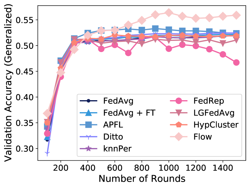
(a) Shakespeare

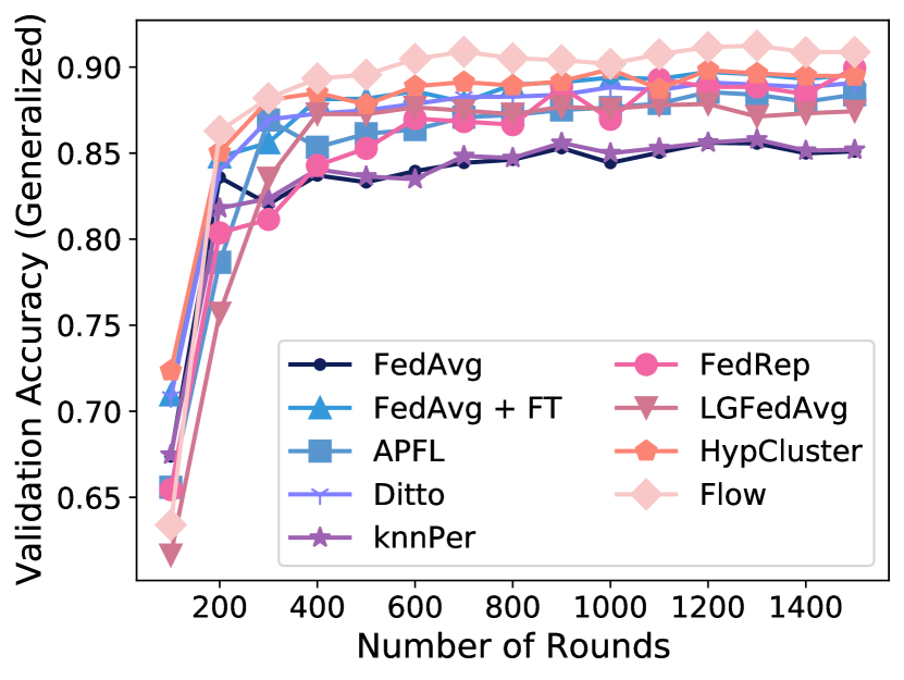
(b) EMNIST

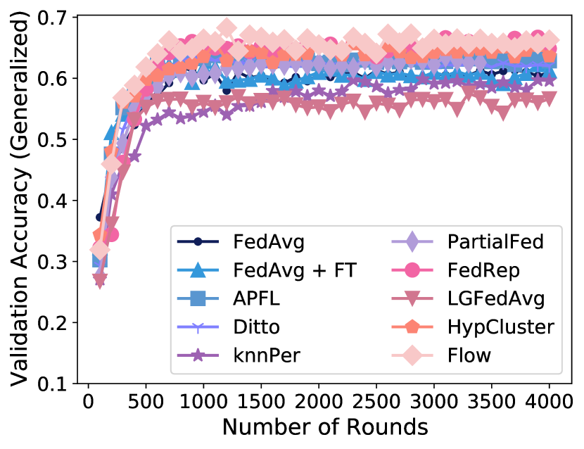
(c) CIFAR10 (0.1)

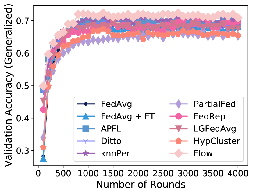
(d) CIFAR 10 (0.6)

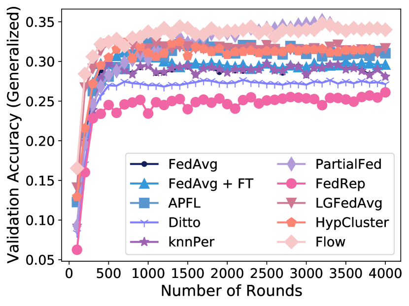
(e) CIFAR100 (0.1)

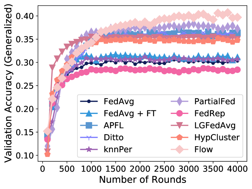
(f) CIFAR100 (0.6)

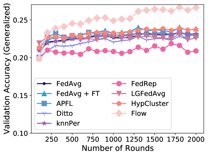
(g) Stackoverflow

Figure 5: Learning curves on Generalized Accuracy Metric of Flow and its baselines.

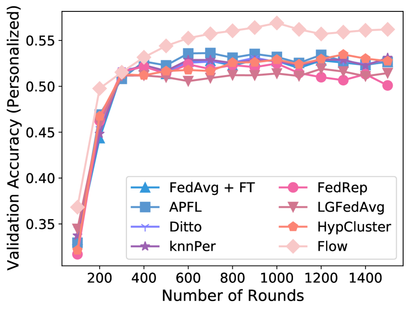
(a) Shakespeare

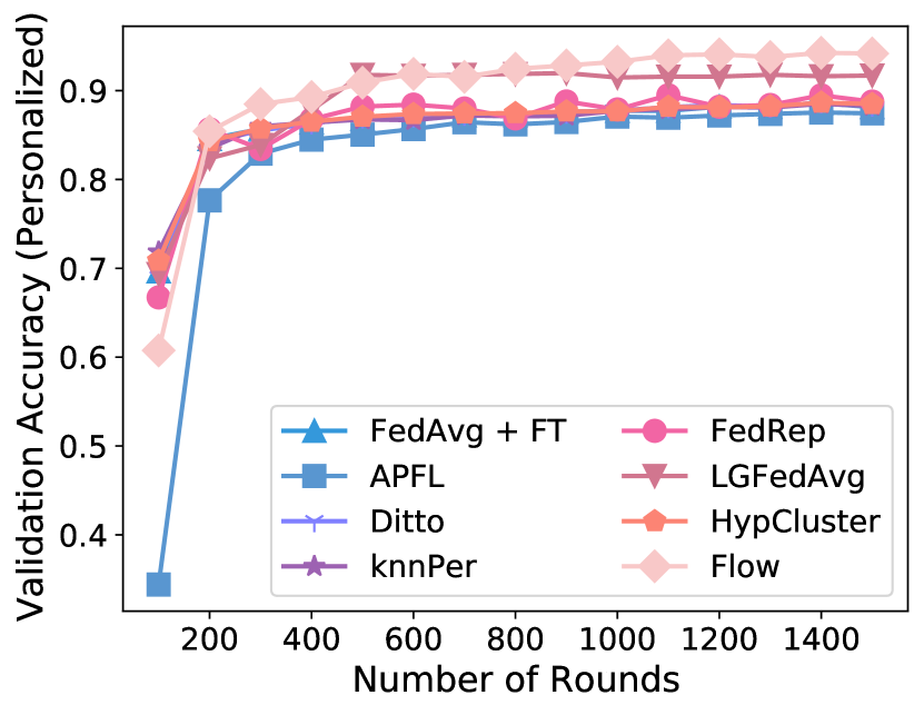
(b) EMNIST

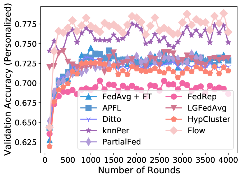
(c) CIFAR10 (0.1)

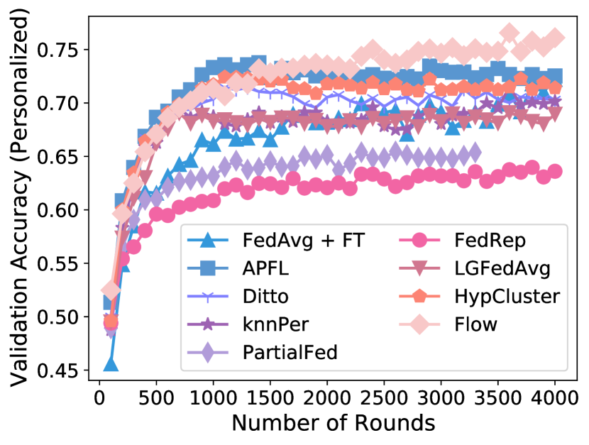
(d) CIFAR 10 (0.6)

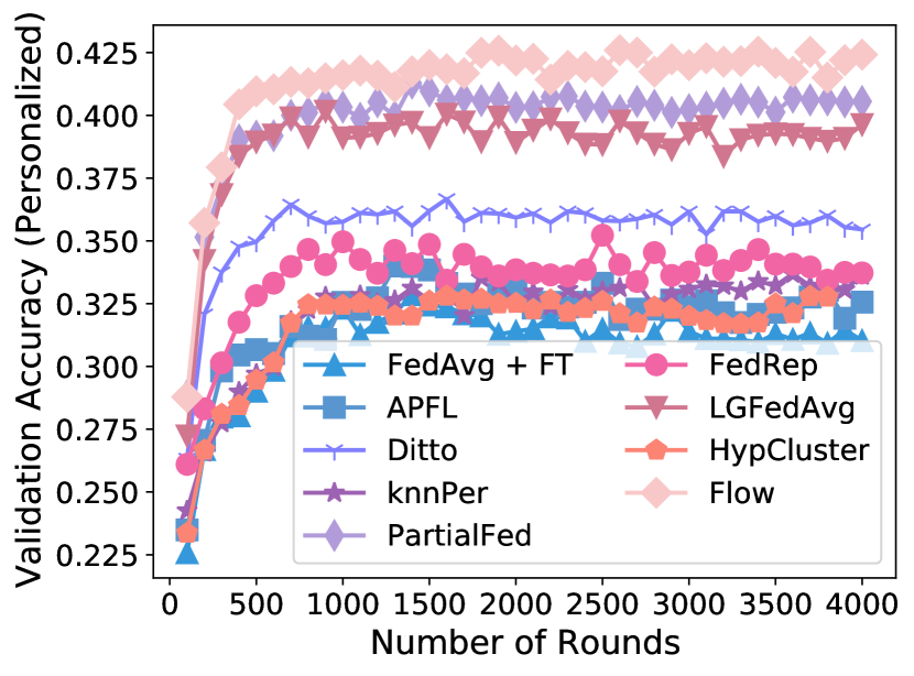
(e) CIFAR100 (0.1)

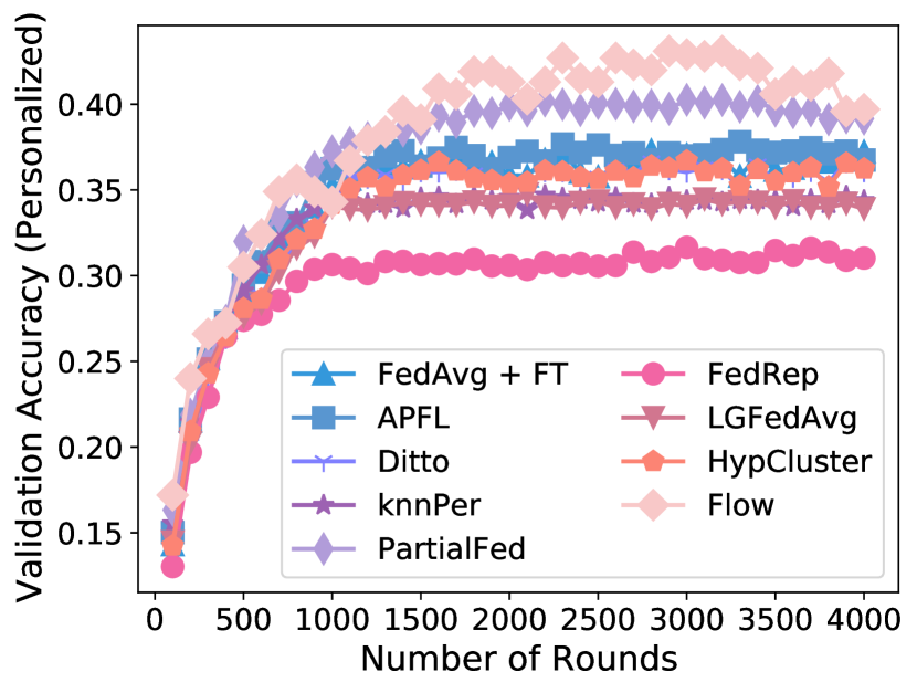
(f) CIFAR100 (0.6)

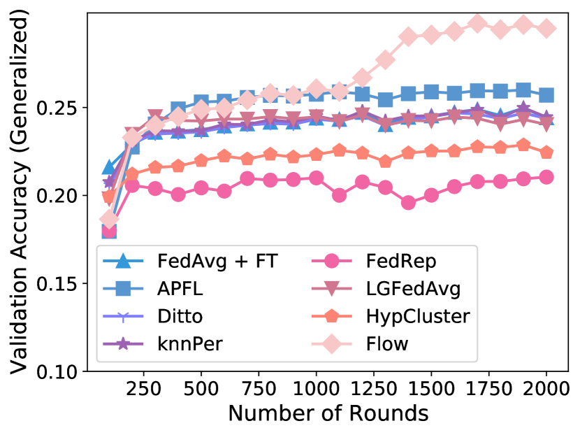
(g) Stackoverflow

Figure 6: Learning curves on Personalized Accuracy Metric of Flow and its baselines.

Flow sees an improvement of 1.11-3.46% in $Acc_{g}$ and 1.33-4.58% in $Acc_{p}$ over the best performing baseline. Besides the main observations listed in Section 5, we discuss results on the CIFAR100 dataset here. For CIFAR100 (0.6), Flow (40.08% $\pm$ 0.27%) matches the personalized accuracy of the highest performing baseline, PartialFed (40.18% $\pm$ 0.19%), while achieving $1.98\%$ point increase in generalized accuracy. And for CIFAR100 (0.1), Flow improves personalized accuracy by $1.78\%$ points. For generalized accuracy, Flow ($34.00\%\pm 0.32\%$) reaches close to the best performing baseline, PartialFed ($34.79\%\pm 0.29\%$). The reason behind the on-par performance of Flow with PartialFed can be attributed to the statefulness of PartialFed. With the assumption of full device participation, PartialFed makes use of each client’s previous state of the personalized model to further train its layer-wise model building policy. With Flow, both the assumptions of full device participation and statefulness of the personalized model are not necessary. Since the clients do not necessarily have to carry their personalized model states to the upcoming rounds, the personalized model recreated by Flow might be unable to compete against stateful approaches like PartialFed. Although because of the per-instance routing, Flow still manages to outperform PartialFed for the CIFAR10 (0.1/0.6) datasets, and gives comparable performance for the CIFAR100 (0.1/0.6) datasets.

D.2 Effectiveness of the Alternative Training of the Global Model

We experimented with three modes of training for the global model: (a) Global model trained first, then the policy module, (b) Policy module trained first, then the global model, (c) Global model and Policy module trained alternatively. The results are shown in Figure 9. We see that the alternate training results in a more stable training compared to the other two modes of training. These results are in conformance with other works [49, 50] which have also used alternative training for policy and model weights training.

D.3 Dataset Split

We experimented with the Stackoverflow Next Word Prediction task on initial rounds for the local and global training dataset splits. The plot is shown in Figure 9. We observe that for the dataset split size of 0.75:0.25 for local and global datasets respectively, the global model does not get sufficient samples to converge, resulting in worse personalized model performance since the personalized model is based on the global model. While a split of 0.25:0.75 for local and global datasets has closer performance to that of a 0.50:0.50 split, lesser data (and hence fewer iterations) to the local model leads to local model weights being similar to that of global model, diminishing the impact of personalization.

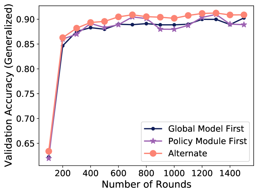
Figure 7: Results for different modes of training for EMNIST
a
a

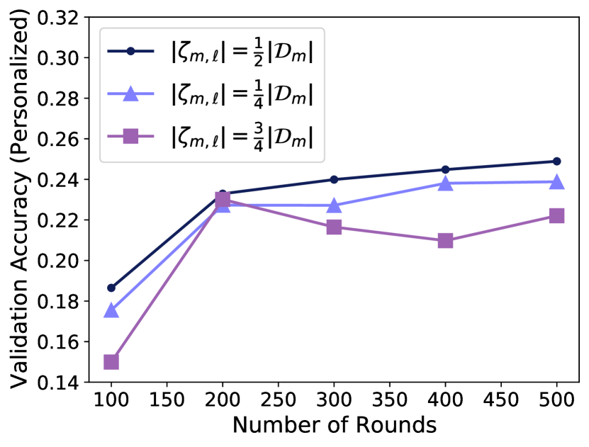
Figure 8: Earlier stages of Stackoverflow NWP training with different local:global dataset splits

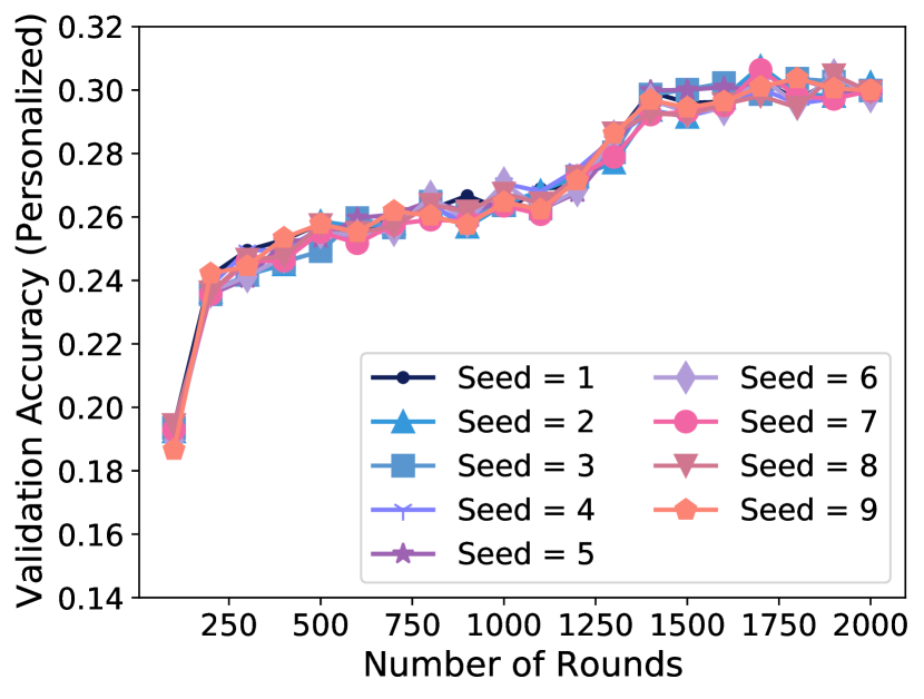
Figure 9: Stackoverflow NWP training with seed choices of [1,9]
a

D.4 More Seeds

We have re-run Stackoverflow experiment with seeds in {1, 2, 3, 4, 5 , 6, 7, 8, 9}, the results show no material difference. See Figure 9.

D.5 Percentage of Clients Benefiting from Personalization

In this section we discuss the effect of personalization, by comparing each client’s performance on their individual personalized models with their performance on the global model. The evaluation, just as in section D.1, is done on the test datasets of all the clients. The goal with any personalization method is to make each client’s personalized model more beneficial (for us, in terms of accuracy) compared to the global model. Hence we want $Acc_{p}>Acc_{g}$, to incentivize personalization for each client. As shown in Table 7, compared to the best performing baseline, Flow improves the utility of personalization by up to 3.31% points.

Table 7: % of clients for which $Acc_{p}>Acc_{g}$ (the higher, the better).

	Stackoverflow	EMNIST	Shakespeare	CIFAR10 (0.1)	CIFAR100 (0.1)	CIFAR10 (0.6)	CIFAR100 (0.6)
FedAvgFT	79.26%	81.48%	79.00%	97.18%	91.74%	99.33%	88.54%
knnPer	82.73%	89.97%	68.87%	90.00%	94.71%	90.00%	96.37%
PartialFed	-	-	-	88.30%	90.32%	84.80%	98.64%
APFL	69.66%	93.39%	79.22%	87.48%	86.18%	90.63%	92.03%
Ditto	74.59%	79.26%	73.74%	90.52%	91.45%	89.61%	97.45%
FedRep	91.53%	82.20%	79.78%	92.30%	78.81%	84.64%	99.54%
LGFedAvg	83.47%	66.16%	88.43%	88.41%	86.39%	89.59%	91.73%
HypCluster	80.46%	80.70%	74.84%	95.11%	93.70%	98.18%	99.73%
Flow (Ours)	92.74%	96.70%	89.77%	98.33%	97.29%	99.62%	99.75%

D.6 Breakdown of Correctly Classified Instances

Here we show a detailed view of how instances (across all the clients) get classified correctly between global and personalized models for each of the baselines. For the plots in Figures 10, $y$-axis represent % of instances correctly classified by (a) Both the global and the personalized models (both-correct), (b) Only the global model (global-only), and (c) Only the personalized model (personalized-only). This % of instances metric is averaged across all clients, and is based on their test datasets. The goal here is to increase the % of instances for both-correct and personalized-only, and reduce the % of instances for global-only.

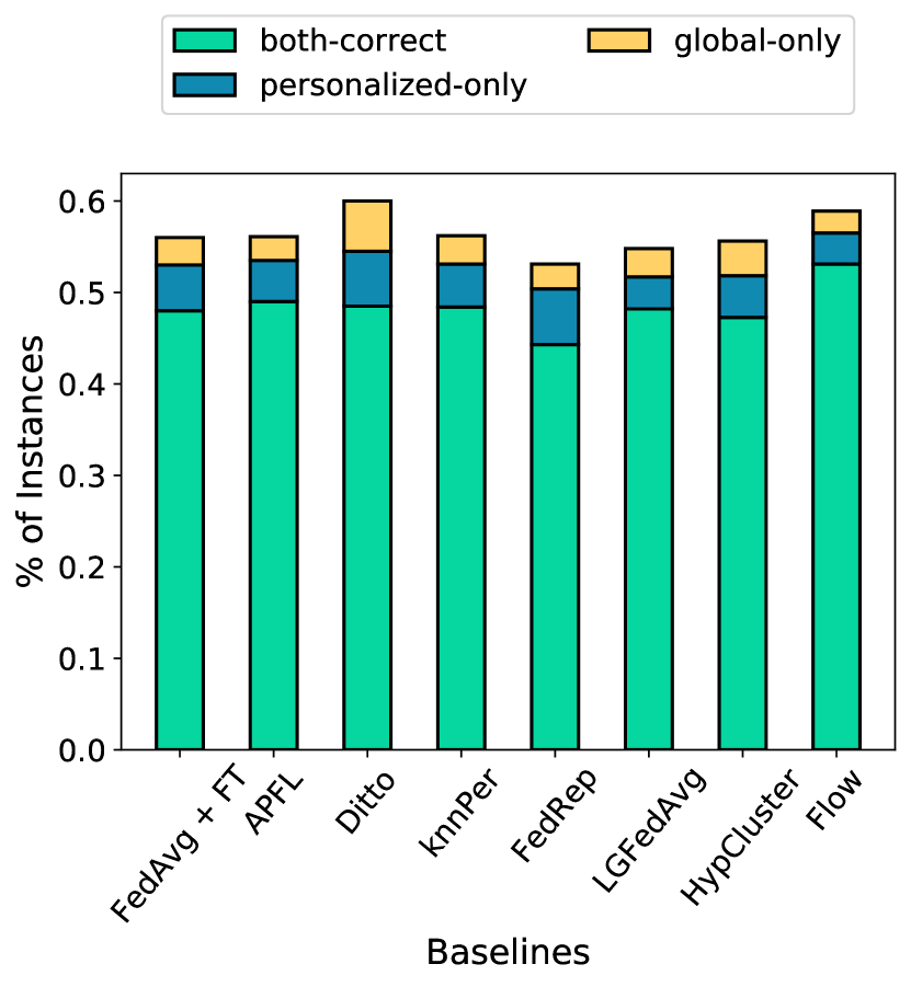
(a) Shakespeare

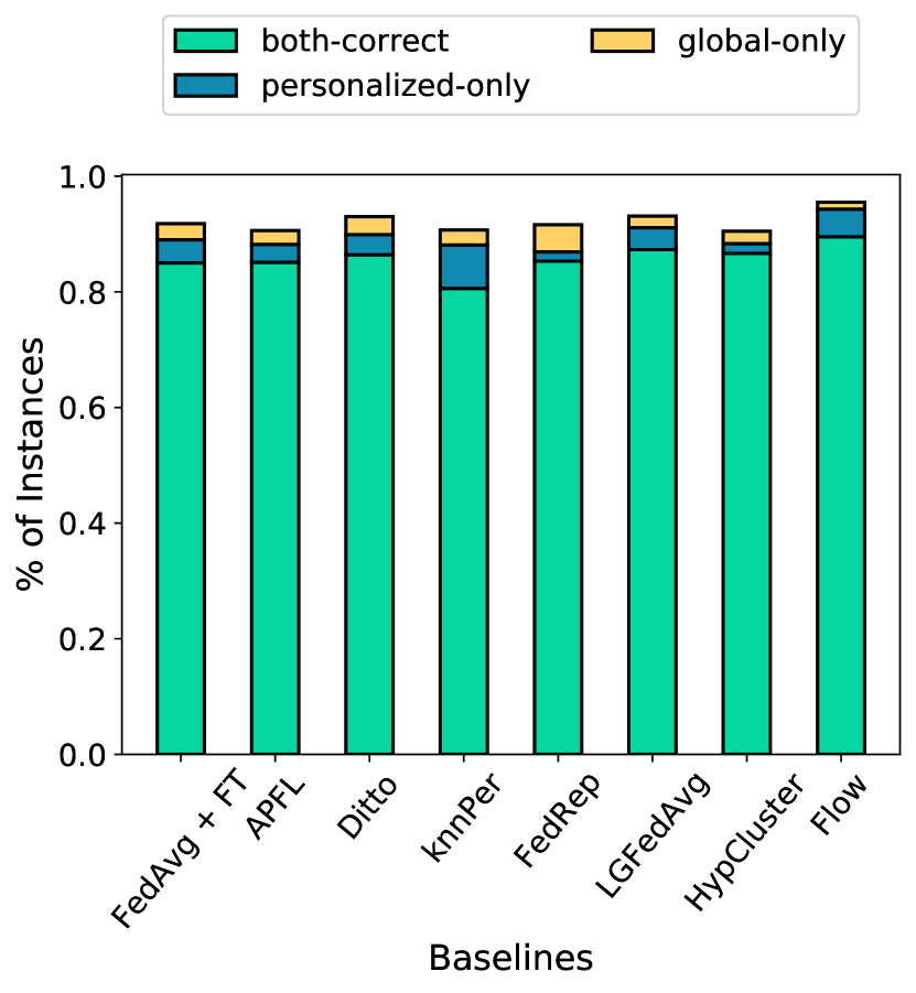
(b) EMNIST

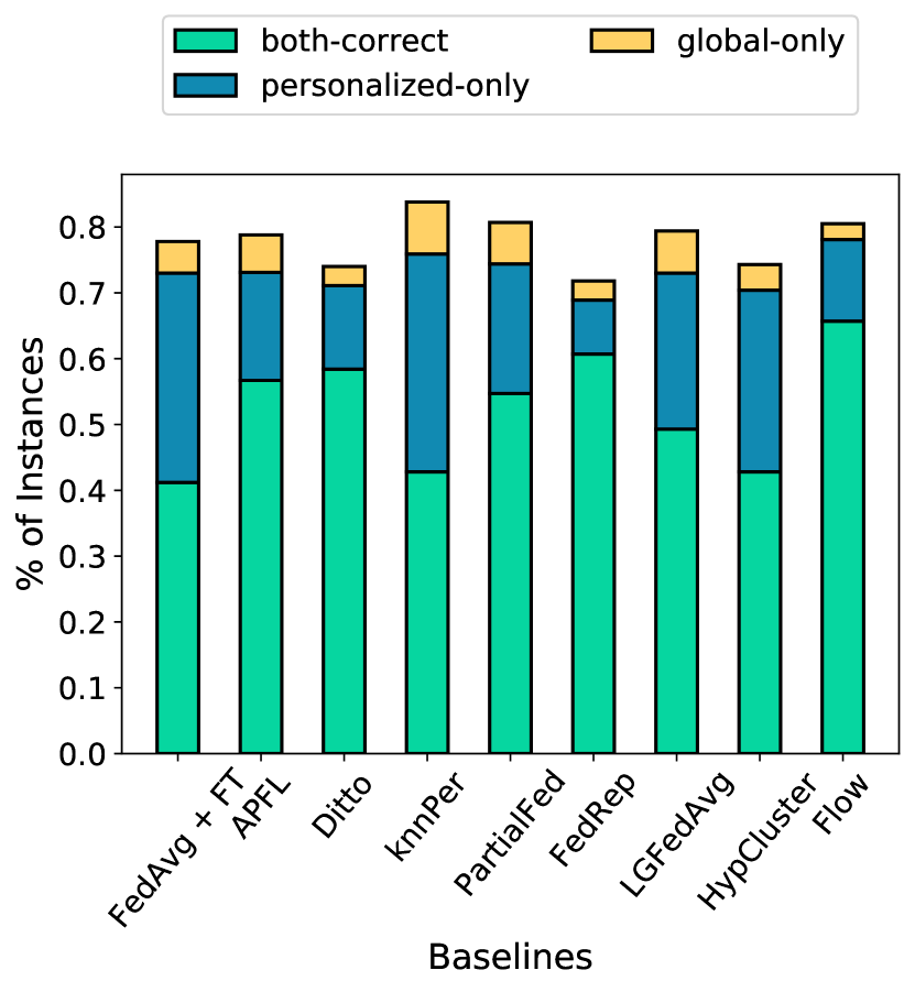
(c) CIFAR10 (0.1)

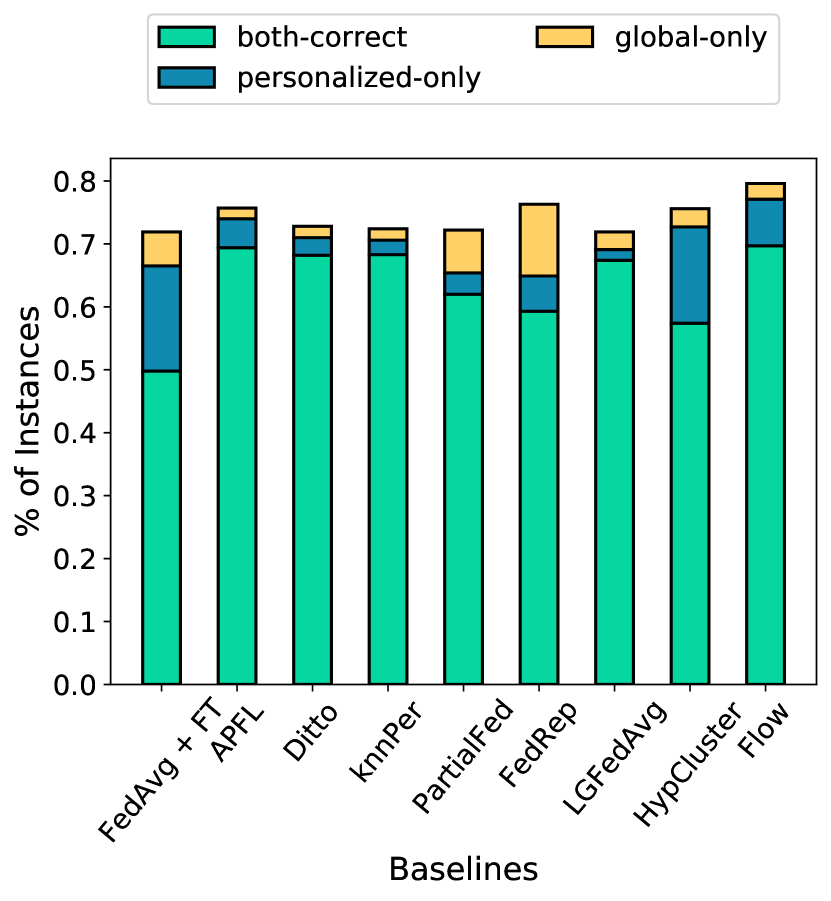
(d) CIFAR 10 (0.6)

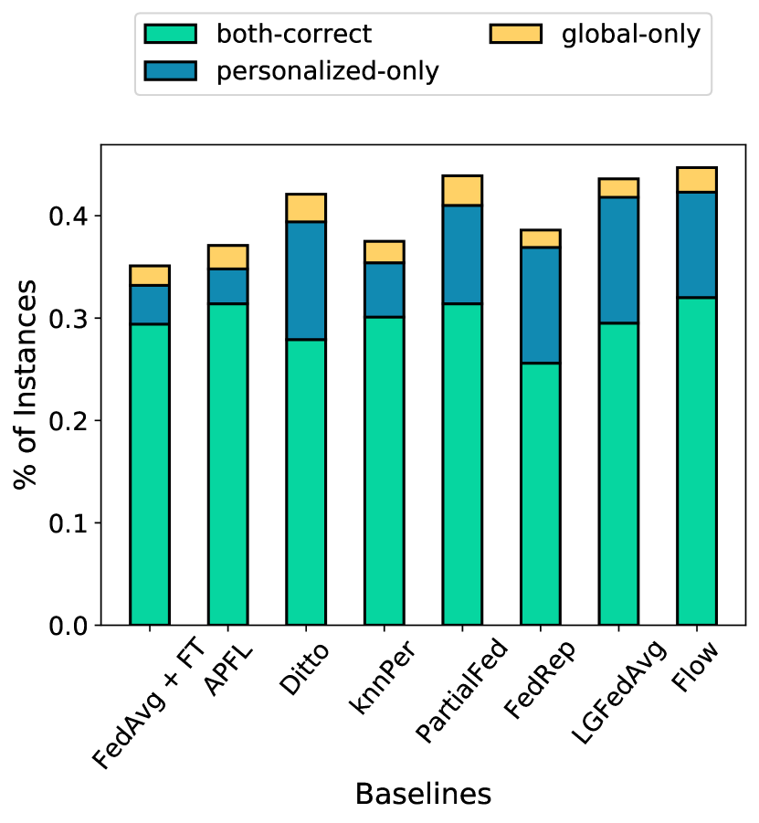
(e) CIFAR100 (0.1)

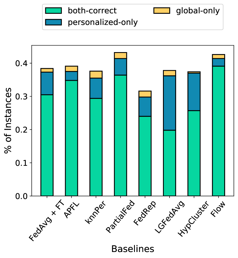
(f) CIFAR100 (0.6)

Figure 10: Different combinations of $w_{g}$ and $w_{p}$ accuracies.

We make the following observations for each of the datasets: Since Flow improves both the generalized and personalized accuracies, we see higher both-correct for Stackoverflow (by 2.75% points), Shakespeare (by 4.34% points), EMNIST (by 3.17% points), CIFAR10 (0.1) (by 5.24% points), CIFAR10 (0.6) (by 0.03% points), CIFAR100 (0.1) (by 0.63% points) and CIFAR100 (0.6) (by 2.78% points).

Due per-instance personalization, we see improvements in personalized accuracy, but those improvements are also included in the both-correct bars, so solely comparing personalized-only bar lengths is not a right comparison. Similarly, we see fewer instances in global-only bars due to the increase in instances which fall under both-correct.

D.7 Analysis of Routing Decisions

Now we show probability value analysis of the routing policy for CIFAR10/100 datasets. Here we have fixed the client as the client which had the highest loss difference between its global and personalized models for Flow. This analysis was done during the inference stage, on the test dataset of the above-mentioned client. The box plots show statistics on the probability of picking the global route for all the instances. Echoing the observations made in Section 5, in Figure 11, we see a trend in increasing probability for the global parameters for the instances which are correctly classified by only the global model. In the contrary, for the instances which can only be classified by the personalized model, the probability for taking the global route is lower as the input passes through more layers.

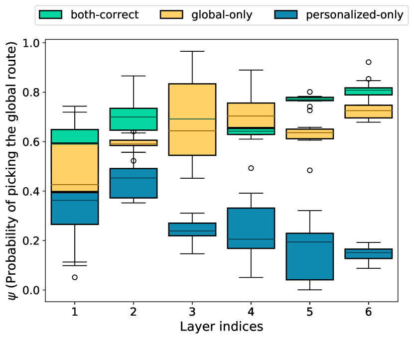
(a) CIFAR10 (0.1)

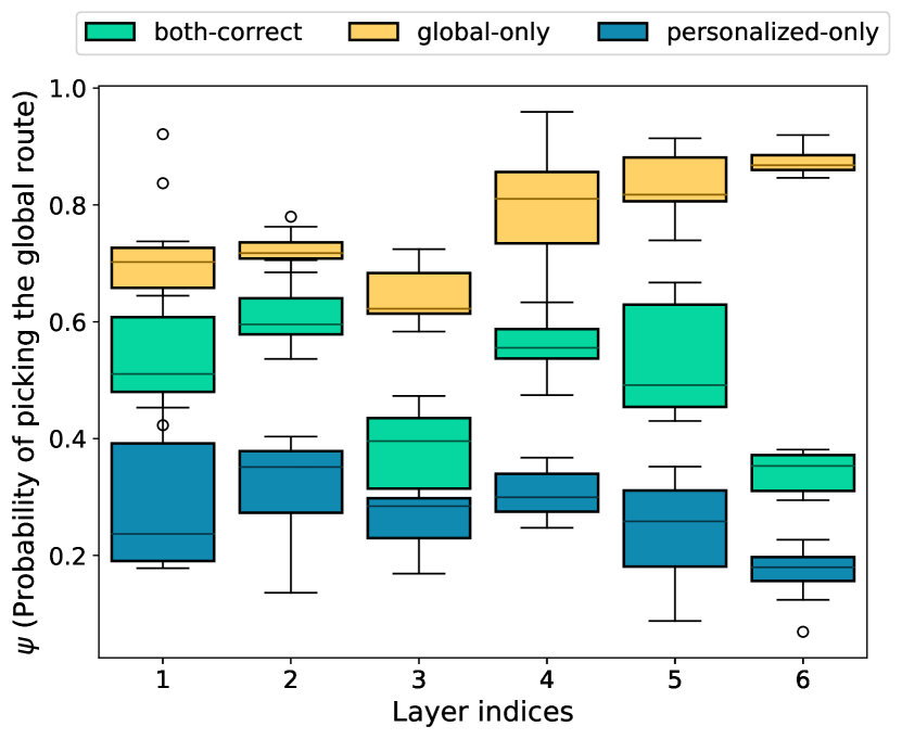
(b) CIFAR 10 (0.6)

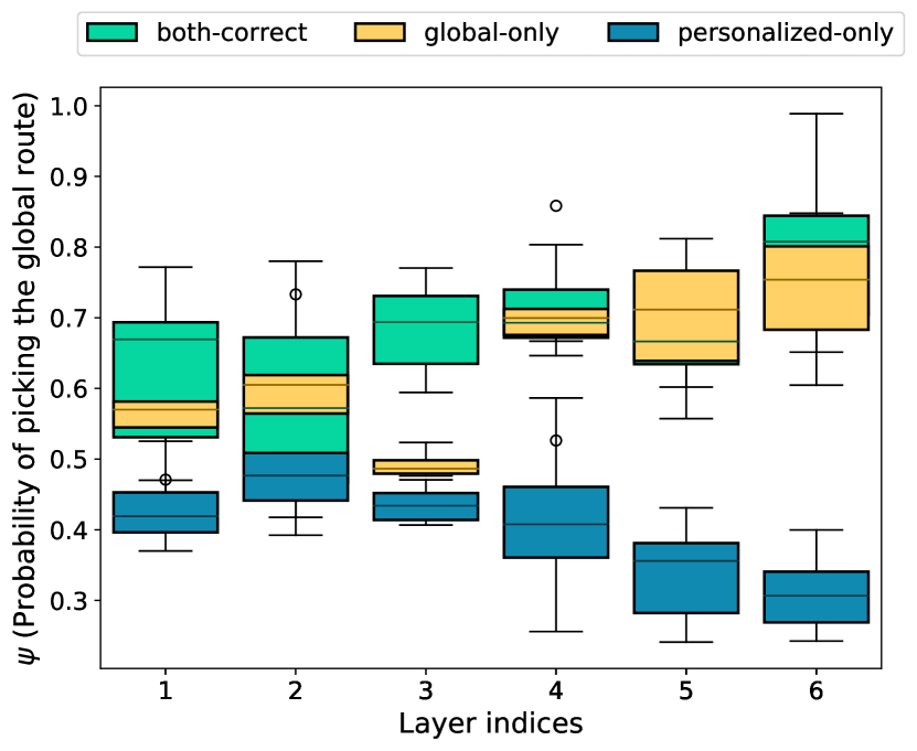
(c) CIFAR100 (0.1)

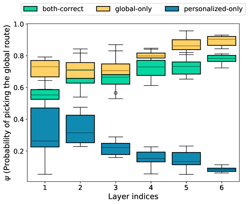
(d) CIFAR100 (0.6)

Figure 11: Behavior of $\psi_{g}$ for all instances with respect to each layer of a client with highest loss difference between personalized and global models.

D.8 Ablation Study: Regularization

Figures 12 and 13 show the validation curves for generalized and personalized accuracy with and without the regularization term used in the policy learning objective as shown in Equation 4. With regularization, we see an improvement of 2.18% (Stackoverflow), 1.86% (Shakespeare), 3.98% (EMNIST), 2.55% (CIFAR10 0.1), 4.36% (CIFAR10 0.6), 0.91% (CIFAR100 0.1), 3.46% (CIFAR100 0.6) for the generalized accuracy. And for the personalized accuracy, we see an improvement of 1.92% (Stackoverflow), 2.02% (Shakespeare), 3.01% (EMNIST), 0.65% (CIFAR10 0.1), 3.98% (CIFAR10 0.6), 2.42% (CIFAR100 0.1), 2.19% (CIFAR100 0.6).

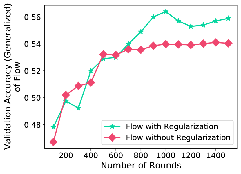
(a) Shakespeare

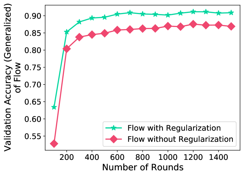
(b) EMNIST

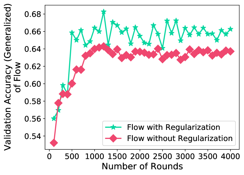
(c) CIFAR10 (0.1)

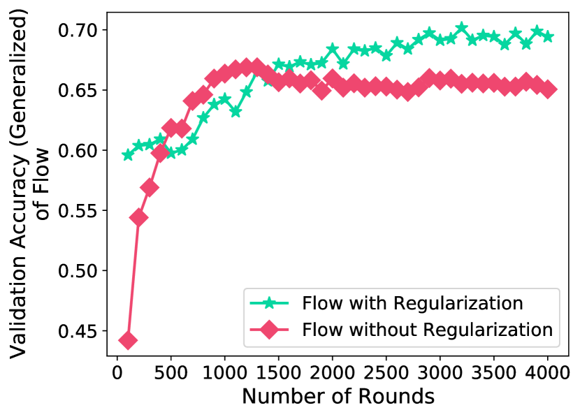
(d) CIFAR 10 (0.6)

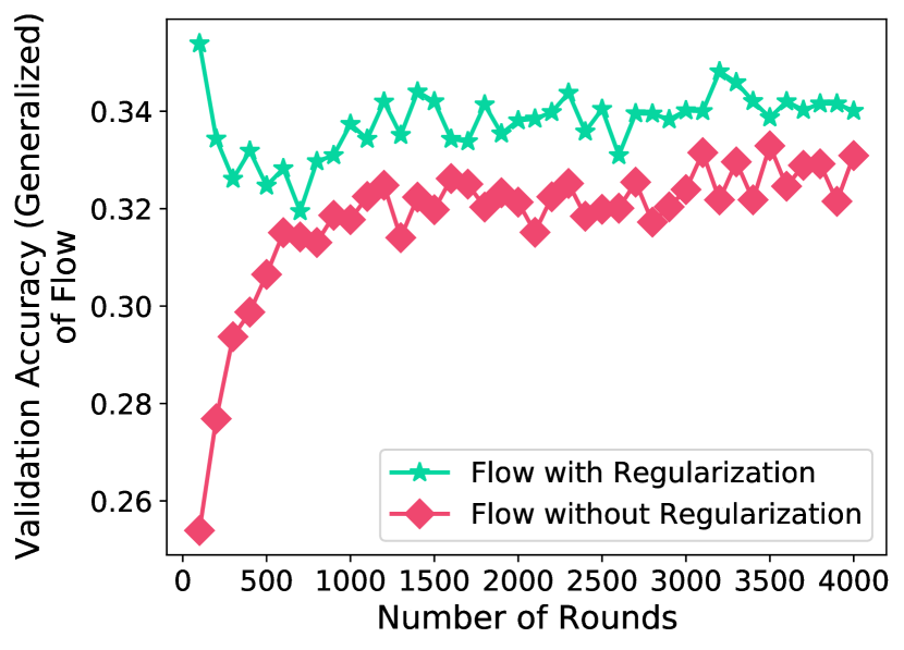
(e) CIFAR100 (0.1)

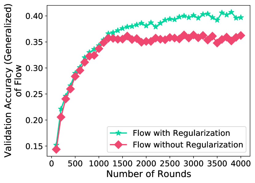
(f) CIFAR100 (0.6)

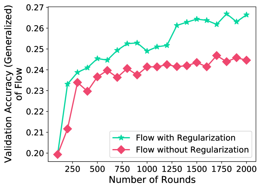
(g) Stackoverflow

Figure 12: Generalized accuracy of the ablation study on the regularization term used in the policy learning objective.

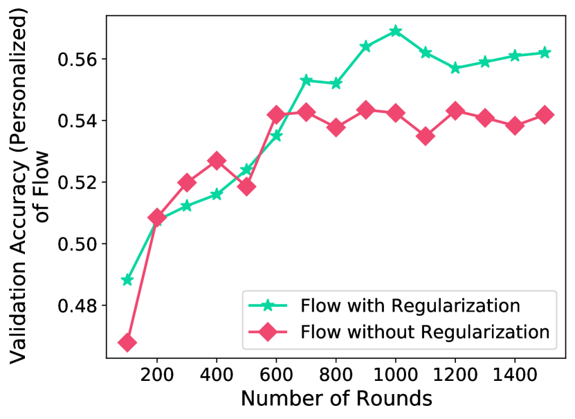
(a) Shakespeare

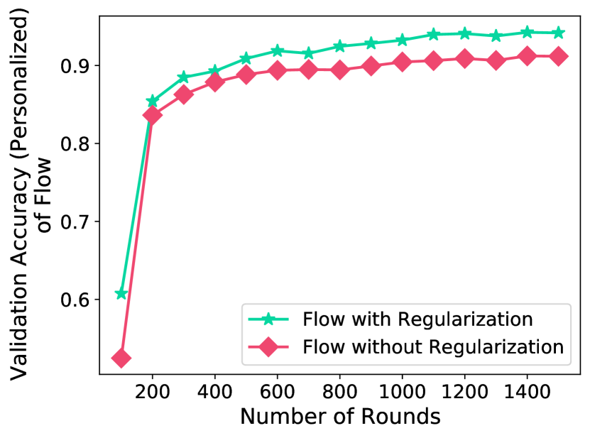
(b) EMNIST

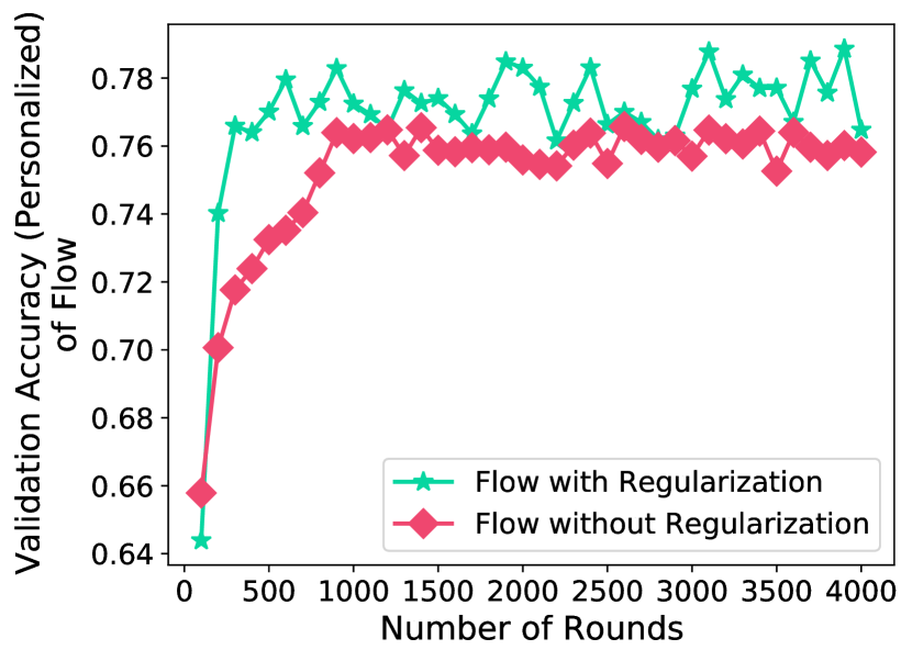
(c) CIFAR10 (0.1)

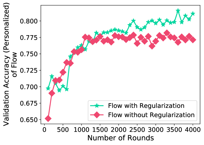
(d) CIFAR 10 (0.6)

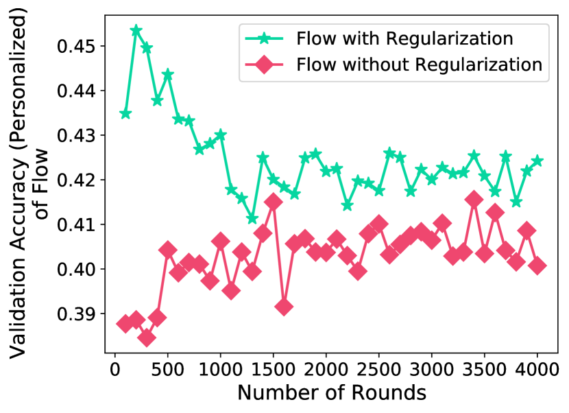
(e) CIFAR100 (0.1)

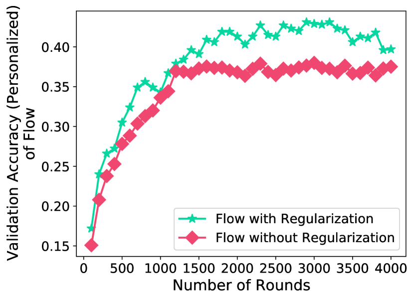
(f) CIFAR100 (0.6)

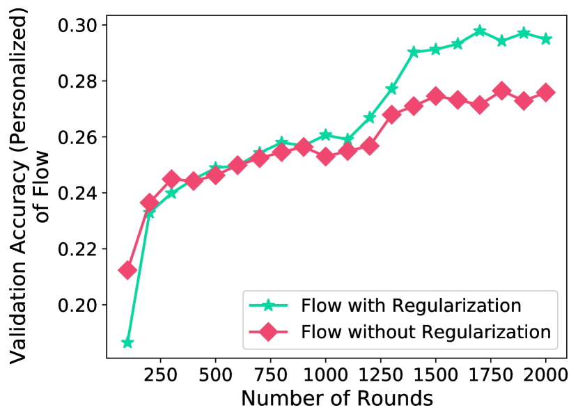
(g) Stackoverflow

Figure 13: Personalized accuracy of the ablation study on the regularization term used in the policy learning objective.

D.9 Ablation Study: Per-instance Personalization

Figure 14 show the validation curves for 3 Flow variants: (a) Per-instance Per-client Flow, which is the primary design proposed in this work, (b) Per-instance Flow, which makes choices between two global routes solely based on each client’s instances, (c) Per-client Flow, which is simply FedAvgFT where the personalization only depends on a client, and not on any specific instances.

With all the datasets, we see a trend of Per-instance Flow outperforming Per-client Flow by 1.88% (Stackoverflow), 0.82% (Shakespeare), 5.07% (EMNIST), 2.90% (CIFAR10 0.1), 2.41% (CIFAR10 0.6), 7.52% (CIFAR100 0.1), 1.09% (CIFAR100 0.6). We also see the trend of Per-instance Flow outperforming Per-Instance Per-Client Flow by 3.19% (Stackoverflow), 1.24% (Shakespeare), 0.94% (EMNIST), 0.55% (CIFAR10 0.1), 4.49% (CIFAR10 0.6), 3.88% (CIFAR100 0.1), 1.37% (CIFAR100 0.6).

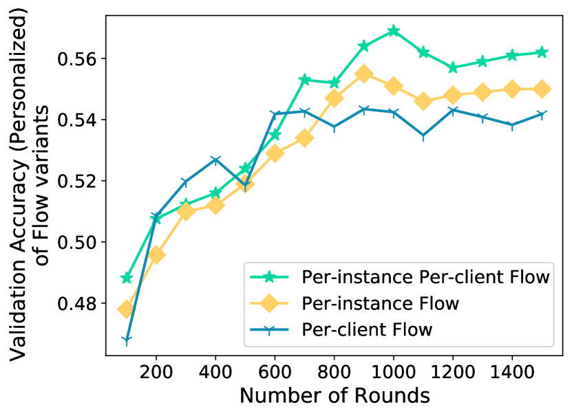
(a) Shakespeare

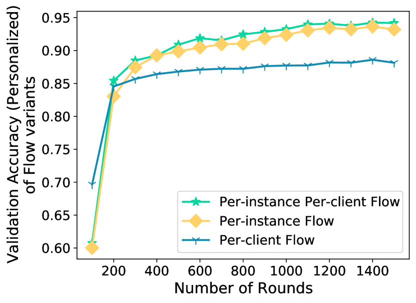
(b) EMNIST

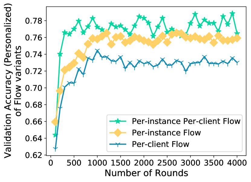
(c) CIFAR10 (0.1)

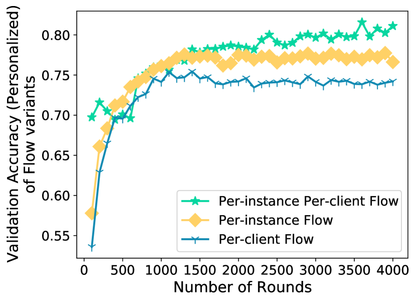
(d) CIFAR 10 (0.6)

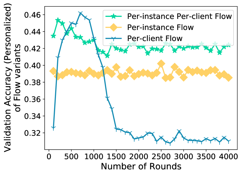
(e) CIFAR100 (0.1)

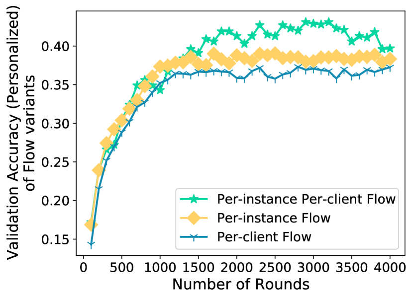
(f) CIFAR100 (0.6)

(g) Stackoverflow

Figure 14: Ablation of the dynamic routing component (Per-client Flow), and the local component (Per-instance Flow).

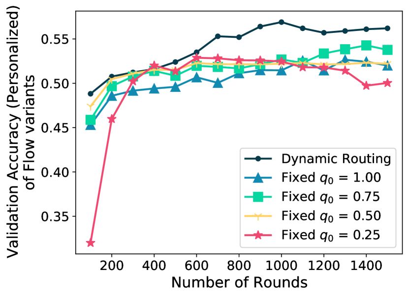
(a) Shakespeare

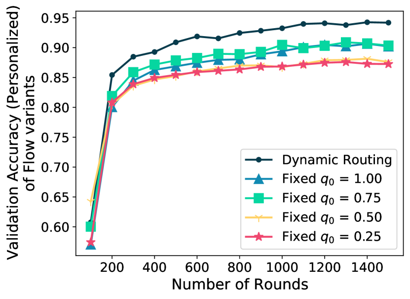
(b) EMNIST

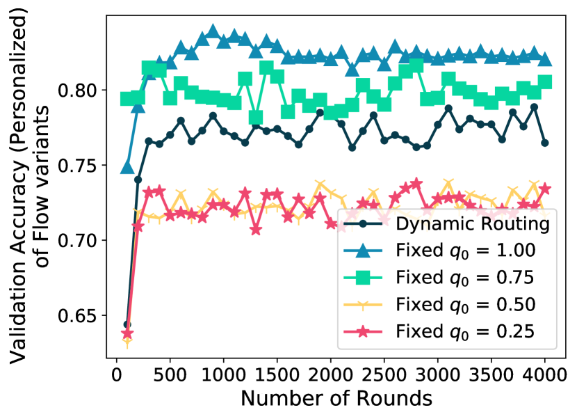
(c) CIFAR10 (0.1)

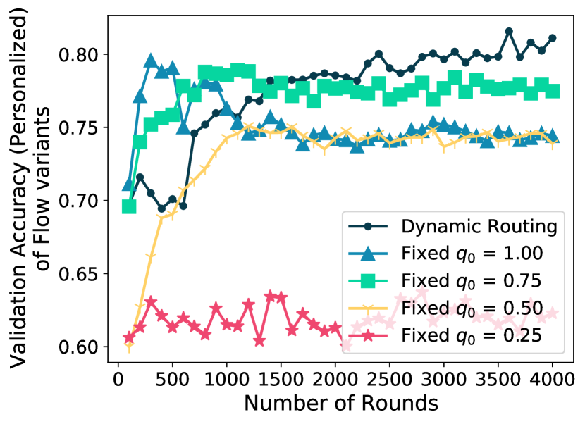
(d) CIFAR 10 (0.6)

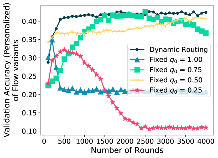
(e) CIFAR100 (0.1)

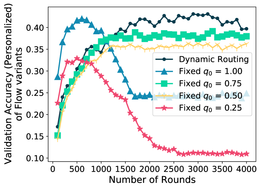
(f) CIFAR100 (0.6)

(g) Stackoverflow

Figure 15: Personalized Accuracy of the Ablation Study on the Dynamic Routing Component.

D.10 Ablation Study: Soft versus Hard Policy

Table 8 shows the personalized accuracy of the test clients while using soft and hard policies during inference. We see that the accuracy difference between the two designs are statistically insignificant. Hence, using a hard policy for inference not only saves half the compute resources, but also doesn’t affect the personalized model’s performance.

D.11 Ablation Study: Dynamic Routing

The accuracy curves are given in Figure 15. The curves show that the phenomena of “dynamic probabilities based on each instance works consistently better than the fixed probabilities for all the clients throughout the training” is indeed observable across all the datasets. The intuition behind that is discussed in Section 5.2, under “Dynamic Routing”.

Table 8: Test (personalized) accuracy of two of the Flow variants: (a) Soft Policy variant where the probability $\mathbf{q}$ is continuous in the range of $[0,1]$ during inference. (b) Hard Policy variant where the probability $\mathbf{q}$ is discrete over the set {0,1} during inference.

Datasets	Stackoverflow	Shakespeare	EMNIST
Soft Policy	29.57% $\pm$ 0.22%	57.01% $\pm$ 0.53%	94.97% $\pm$ 1.06%
Hard Policy	29.49% $\pm$ 0.28%	56.20% $\pm$ 0.49%	94.18% $\pm$ 1.21%

Datasets	CIFAR 10 (0.1)	CIFAR 100 (0.1)	CIFAR 10 (0.6)	CIFAR 100 (0.6)
Soft Policy	77.24% $\pm$ 1.30%	42.75% $\pm$ 0.30%	77.02% $\pm$ 0.90%	39.74% $\pm$ 0.13%
Hard Policy	76.47% $\pm$ 1.25%	42.42% $\pm$ 0.36%	77.11% $\pm$ 0.86%	40.08% $\pm$ 0.27%

Appendix E Proofs

E.1 Flow: Detailed

Here we give a detailed version of Flow (Algorithm 2) for proving its convergence properties. Here we are assuming that the global and local model output interpolation is model-wise (after the final layer), not layer-wise.

Input: $R$: Total number of rounds, $r\in[R]$: Round index, $M$: Total number of clients, $m\in[M]$: Client index, $\mathcal{M}{}$: Set of available clients , $p$: Client sampling rate, $K$: Total local epoch count, $k\in[K]$: Epoch index, $\eta_{\ell}$: Local learning rate, $w^{(r)}_{g}$: Global model at $r^{th}$ round, $w^{(r,k)}_{g,m}$: $m^{th}$ client’s local update of the global model for $r^{th}$ round and $k^{th}$ epoch, $w^{(r,k)}_{\ell,m}$: $m^{th}$ client’s local model for $r^{th}$ round and $k^{th}$ epoch, $w^{(r,k)}_{p,m}$: $m^{th}$ client’s personalized model for $r^{th}$ round and $k^{th}$ epoch, $\psi^{(r)}_{g}$: Global policy model at $r^{th}$ round, $\psi^{(r,k)}_{g,m}$: $m^{th}$ client’s routing policy for $r^{th}$ round and $k^{th}$ epoch, $\mathcal{D}_{m}$: Data distribution of $m^{th}$ client, $\mathcal{S}_{m}$: Dataset of $m^{th}$ client, $\zeta_{m,\ell}$: Dataset used to train $w_{\ell}$, $\zeta_{m,g}$: Dataset used to train $w_{g}$ and $\psi_{g}$

Output: $w^{(R+1)}_{g}$: Global model at the end of the training

1 Server randomly initializes $w^{(1)}_{g}$

2 for $r\in[R]$ round do

3       Sample $M$ clients from $\mathcal{M}{}$ with the rate of $p$

4       Send $w^{(r)}_{g}$, $\psi^{(r)}_{g}$ to all the clients

5       for $m\in[M]$ in parallel do

6             $w^{(r,0)}_{g,m}\leftarrow w_{g}^{(r)}$; $\psi^{(r,0)}_{g,m}\leftarrow\psi^{(r)}_{g}$; $w^{(r,0)}_{\ell,m}\leftarrow w^{(r,0)}_{g,m}$

             $\zeta_{m,\ell},\zeta_{m,g}\leftarrow\mathcal{S}_{m}$ /* Creating two mutually exclusive datasets */

7             for $k\in[K_{1}]$ epochs  do

8                   $w^{(r,k)}_{\ell,m}\leftarrow w^{(r,k-1)}_{\ell,m}-\eta_{\ell}\nabla f_{m}(w^{(r,k-1)}_{\ell,m};\zeta_{m,\ell})$

9             end for

10             for $k\in[K_{2}]$ epochs do

11                   $\forall\;(x_{m},y_{m})\sim\zeta_{m,g}$, define $\tilde{w}^{(r,k-1)}_{p,m}(x_{m})\leftarrow\psi^{(r,k-1)}_{g,m}(x_{m})\cdot w^{(r,k-1)}_{g,m}(x_{m})+(1-\psi^{(r,k-1)}_{g,m}(x_{m}))\cdot w^{(r,K)}_{\ell,m}(x_{m})$

12                   $\psi^{(r,k)}_{g,m}\leftarrow\psi^{(r,k-1)}_{g,m}-\eta_{\ell}\nabla_{\psi^{(r,k-1)}_{g,m}}\left[f_{m}(\tilde{w}^{(r,k-1)}_{p,m};\zeta_{m,g})\right]$

13                   $\forall\;(x_{m},y_{m})\sim\zeta_{m,g}$, define $w^{(r,k-1)}_{p,m}(x_{m})\leftarrow\psi^{(r,k)}_{g,m}(x_{m})\cdot w^{(r,k-1)}_{g,m}(x_{m})+(1-\psi^{(r,k)}_{g,m}(x_{m}))\cdot w^{(r,K)}_{\ell,m}(x_{m})$

14                   $w^{(r,k)}_{g,m}\leftarrow w^{(r,k-1)}_{g,m}-\ \eta_{\ell}\nabla_{w^{(r,k-1)}_{g,m}}f_{m}(w^{(r,k-1)}_{p,m};\zeta_{m,g})$

15             end for

16            Send back $w^{(r,K)}_{g,m}$, $\psi^{(r,K)}_{g,m}$, $n_{m}$ := $|\zeta_{m,g}|$

17       end for

18      $w^{(r+1)}_{g}\leftarrow\frac{1}{nM}\sum_{m\in[M]}n_{m}w^{(r,K)}_{g,m}$

19       $\psi^{(r+1)}_{g}\leftarrow\frac{1}{nM}\sum_{m\in[M]}n_{m}\psi^{(r,K)}_{g,m}$

20 end for

Algorithm 2 Flow

E.2 Basics

We perform theoretic analysis of Flow based on the following setup: There are total $M$ clients. A client is denoted by a unique integer $m$ associated with it where $m\in[M]$. Each client $m$ has a dataset $\mathcal{S}_{m}=\{(x_{m}^{(i)},y_{m}^{(i)});i\in[n_{m}]\}$ where $(x_{m}^{(i)},y_{m}^{(i)})$ has been sampled from $\mathcal{D}_{m}$ distribution of the $m^{th}$ client. $n_{m}=|\mathcal{S}_{m}|$ is the total sample count of the $m^{th}$ client. Total sample count across all the participating client is $n=\sum_{m\in[M]}n_{m}$. The ratio of $m^{th}$ client’s sample count to total sample count is $\alpha=\frac{n_{m}}{n}$.

The global distribution is defined as $\mathcal{D}=\sum_{m\in[M]}q_{m}\mathcal{D}_{m}$ where $q_{m}$ is the weight associated with $m^{th}$ client and $\sum_{m\in[M]}q_{m}=1$.

Note that $w_{p,m}$ is a combination of outputs of $w_{g,m}$ (Global parameters) and $w_{\ell,m}$ (Local parameters) on each layer. For tractability of analysis, we will assume that the combination is only after the last layer. Hence,

$$w_{p,m}(x_{m})\leftarrow\psi_{g,m}(x_{m})w_{g,m}(x_{m})+(1-\psi_{g,m}(x_{m}))w_{\ell,m}(x_{m}).$$

The local model update rule is,

$$w^{(r,k)}_{\ell,m}\leftarrow w^{(r,k-1)}_{\ell,m}-\eta_{\ell}\nabla f_{m}(w^{(r,k-1)}_{\ell,m}(x_{m}),y_{m})$$

where $w^{(r,0)}_{\ell,m}=w^{(r,0)}_{g,m}=w^{(r)}_{g}$. Indices $r\in[R]$ and $k\in[K]$ are the global round and the local epoch indices.

The policy update rule is,

$$\psi^{(r,k)}_{g,m}\leftarrow\psi^{(r,k-1)}_{g,m}-\eta_{\ell}\nabla_{\psi_{g}}f_{m}(w^{(r,k-1)}_{p,m}(x_{m}),y_{m}).$$

The global model update rule is,

$$w^{(r,k)}_{g,m}\leftarrow w^{(r,k-1)}_{g,m}-\eta_{\ell}\nabla_{w_{g}}f_{m}(w^{(r,k-1)}_{p,m}(x_{m}),y_{m}).$$

We list out all the optimization problems relevant to Flow:

• Local true risk of the personalized model

  $$F_{m}(w_{p,m}):=\mathbb{E}_{(x_{m},y_{m}\sim\mathcal{D}_{m})}[f_{m}(w_{p,m}(x_{m}),y_{m})]$$

  where $f_{m}$ is a loss function associated with the $m^{th}$ client.

• Local empirical risk of the personalized model

  $$\hat{F}_{m}(w_{p,m}):=\frac{1}{n_{m}}\sum_{i\in[n_{m}]}f_{m}(w_{p,m}(x^{(i)}_{m}),y^{(i)}_{m})$$

• Local true risk of the global model

  $$F_{m}(w_{g,m}):=\mathbb{E}_{(x_{m},y_{m}\sim\mathcal{D}_{m})}[f_{m}(w_{g,m}(x_{m}),y_{m})]$$

• Local empirical risk of the global model

  $$\hat{F}_{m}(w_{g,m}):=\frac{1}{n_{m}}\sum_{i\in[n_{m}]}f_{m}(w_{g,m}(x^{(i)}_{m}),y^{(i)}_{m})$$

• Local minimizer of local empirical risk of the personalized model

  $$w_{p,m}^{*}\in\mathcal{H}\text{ such that }\hat{F}_{m}(w_{p,m})\geq\hat{F}_{m}(w_{p,m}^{*});\;\forall w_{p,m}\in\mathcal{H},\;\exists\epsilon>0,\;||w_{p,m}-w_{p,m}^{*}||<\epsilon$$

• Global true risk of the global model

  $$F(w_{g})=\frac{1}{nM}\sum_{m\in[M]}n_{m}\mathbb{E}_{(x_{m},y_{m})\sim\mathcal{S}_{m}}[f_{m}(w_{g,m}(x_{m}),y_{m})]\text{ where }n=|\mathcal{S}|=|\bigcup_{m\in[M]}\mathcal{S}_{m}|$$

• Global empirical risk of the global model

  $$\hat{F}(w_{g})=\frac{1}{nM}\sum_{m\in[M]}n_{m}\hat{F}_{m}(w_{g,m}(x_{m}),y_{m})=\frac{1}{nM}\sum_{m\in[M]}\sum_{i\in[n_{m}]}f_{m}(w_{g,m}(x_{m}^{(i)}),y_{m}^{(i)})$$

• Local minimizer of global empirical risk

  $$w_{g}^{*}\in\mathcal{H}\text{ such that }\hat{F}(w_{g})\geq\hat{F}(w_{g}^{*});\;\forall w_{g}\in\mathcal{H},\;\exists\epsilon>0,\;||w_{g}-w_{g}^{*}||<\epsilon$$

We also use the following assumptions similar to [11, 18, 6]:

Assumption E.1 (Strong Convexity).

$f_{m}$ is $\mu$-convex for $\mu\geq 0$. Hence,

$$\left<\nabla f_{m}(w),v-w\right>\leq f_{m}(v)-f_{m}(w)-\frac{\mu}{2}||w-v||^{2},\;\forall m\in[M]\text{ and }w,v\in\mathcal{H}.$$

We also generalize our convergence analysis for $\mu=0$, general convex cases.

Assumption E.2 (Smoothness).

The gradient of $f_{m}$ is $\beta$-Lipschitz,

$$||\nabla f_{m}(w)-\nabla f_{m}(v)||\leq\beta||w-v||,\;\forall m\in[M]\text{ and }w,v\in\mathcal{H}.$$

Assumption E.3 (Bounded Local Variance).

$h_{m}(w):=\nabla f_{m}(w(x_{m}),y_{m})$ is an unbiased stochastic gradient of $f_{m}$ with variance bounded by $\sigma_{\ell}^{2}$.

$$\mathbb{E}_{(x_{m},y_{m}\sim\mathcal{D}_{m})}||h_{m}(w)-\nabla f_{m}(w(x_{m}),y_{m})||^{2}\leq\sigma_{\ell}^{2},\;\forall m\in[M]\text{ and }w\in\mathcal{H}.$$

Assumption E.4 (($G,B$)-Bounded Gradient Dissimilarity).

There exists constants $G\geq 0$ and $B\geq 1$ such that

$$\frac{1}{M}\sum_{m\in[M]}||\nabla f_{m}(w)||^{2}\leq G^{2}+2\beta B^{2}(F(w)-F(w^{*}))$$

for a convex $f_{m}$. And for a non-convex $f_{m}$,

$$\frac{1}{M}\sum_{m\in[M]}||\nabla f_{m}(w)||^{2}\leq G^{2}+B^{2}||\nabla F(w)||^{2}.$$

The derivation is given in Section D.1 of Scaffold [18].

We also use a definition to quantify the diversity of a client’s gradient with respect to the global gradient as defined in [29]:

Definition E.5 (Gradient Diversity).

The difference between gradients of the $m^{th}$ client’s true risk and the global true risk based on the global model $w$ is,

$$\delta_{m}=\sup_{w\in\mathcal{H}}||\nabla f_{m}(w)-\nabla F(w)||^{2}$$

E.3 Convergence Proof for the Global Model: Convex (Strong and General) Cases

A client’s local update for one local epoch on the global model, starting with $w^{(r,0)}_{g,m}\leftarrow w^{(r)}_{g}$, is

$$w^{(r,k+1)}_{g,m}=w^{(r,k)}_{g,m}-\eta_{\ell}h_{m}(w^{(r,k)}_{p,m}).$$ (8)

And a client’s local update for $K$ epochs on the global model, would be

$$w^{(r,K)}_{g,m} =w^{(r,0)}_{g,m}-\eta_{\ell}\sum_{k=1}^{K}h_{m}(w^{(r,k-1)}_{p,m})$$ (9)

$$=w^{(r,0)}_{g,m}-\eta_{\ell}\sum_{k=1}^{K}h_{m}(\psi^{(r,k)}_{g,m}(x_{m})w^{(r,k-1)}_{g,m}(x_{m})+(1-\psi^{(r,k)}_{g,m}(x_{m}))w^{(r,K)}_{\ell,m}(x_{m}),y_{m}).$$ (10)

In both the above cases, the gradient is with respect to $w_{g}$ parameters.

The global model update is,

$$w^{(r+1)}_{g}=\frac{1}{nM}\sum_{m\in[M]}n_{m}w^{(r,K)}_{g,m}$$ (11)

We first start with a lemma which binds the deviation between the local model $w^{(r,K)}_{\ell,m}$ and the global model starting point $w^{(r)}_{g}$ for it at round $r$.

Lemma E.6 (Local model progress).

If $m^{th}$ client’s objective function $f_{m}$ satisfies Assumptions E.2, E.3, and condition $\eta_{\ell}\leq\frac{1}{\beta\sqrt{2K(K-1)}}$ in Algorithm 2, the following is satisfied:

$$\mathbb{E}||w^{(r,K)}_{\ell,m}-w^{(r,0)}_{\ell,m}||^{2}\leq 6K^{2}\eta_{\ell}^{2}\mathbb{E}||\nabla f_{m}(w^{(r)}_{g})||^{2}+3K\eta_{\ell}^{2}\sigma_{\ell}^{2}$$

Proof.

$$\mathbb{E}||w^{(r,K)}_{\ell,m}-w^{(r,0)}_{\ell,m}||^{2} =\mathbb{E}||w^{(r,K-1)}_{\ell,m}-\eta_{\ell}\nabla f_{m}(w^{(r,K-1)}_{\ell,m})-w^{(r,0)}_{\ell,m}||^{2}$$ (12)

$$\leq\left(1+\frac{1}{K-1}\right)\mathbb{E}||w^{(r,K-1)}_{\ell,m}-w^{(r,0)}_{\ell,m}||^{2}+K\eta_{\ell}^{2}\mathbb{E}||\nabla f_{m}(w^{(r,K-1)}_{\ell,m})||^{2}+\eta_{\ell}^{2}\sigma_{\ell}^{2}$$ (13)

Here we have used triangle inequality and variance separation.

$$\leq\left(1+\frac{1}{K-1}\right)\mathbb{E}||w^{(r,K-1)}_{\ell,m}-w^{(r,0)}_{\ell,m}||^{2}+K\eta_{\ell}^{2}\mathbb{E}||\nabla f_{m}(w^{(r,K-1)}_{\ell,m})||^{2}+\eta_{\ell}^{2}\sigma_{\ell}^{2}$$ (14)

$$\leq\left(1+\frac{1}{K-1}\right)\mathbb{E}||w^{(r,K-1)}_{\ell,m}-w^{(r,0)}_{\ell,m}||^{2}+\eta_{\ell}^{2}\sigma_{\ell}^{2}$$

$$\qquad+K\eta_{\ell}^{2}\mathbb{E}||\nabla f_{m}(w^{(r,K-1)}_{\ell,m})-\nabla f_{m}(w^{(r,0)}_{\ell,m})+\nabla f_{m}(w^{(r,0)}_{\ell,m})||^{2}$$ (15)

$$\leq\left(1+\frac{1}{K-1}\right)\mathbb{E}||w^{(r,K-1)}_{\ell,m}-w^{(r,0)}_{\ell,m}||^{2}+2K\eta_{\ell}^{2}\mathbb{E}||\nabla f_{m}(w^{(r,K-1)}_{\ell,m})-\nabla f_{m}(w^{(r,0)}_{\ell,m})||^{2}$$

$$\qquad+2K\eta_{\ell}^{2}\mathbb{E}||\nabla f_{m}(w^{(r,0)}_{\ell,m})||^{2}+\eta_{\ell}^{2}\sigma_{\ell}^{2}$$ (16)

$$\leq\left(1+\frac{1}{K-1}\right)\mathbb{E}||w^{(r,K-1)}_{\ell,m}-w^{(r,0)}_{\ell,m}||^{2}+2K\beta^{2}\eta_{\ell}^{2}\mathbb{E}||w^{(r,K-1)}_{\ell,m}-w^{(r,0)}_{\ell,m}||^{2}$$

$$\qquad+2K\eta_{\ell}^{2}\mathbb{E}||\nabla f_{m}(w^{(r,0)}_{\ell,m})||^{2}+\eta_{\ell}^{2}\sigma_{\ell}^{2}$$ (17)

Assuming $\eta_{\ell}\leq\frac{1}{\beta\sqrt{2K(K-1)}}$, we get

$$\mathbb{E}||w^{(r,K)}_{\ell,m}-w^{(r,0)}_{\ell,m}||^{2} \leq\left(1+\frac{2}{K-1}\right)\mathbb{E}||w^{(r,K-1)}_{\ell,m}-w^{(r,0)}_{\ell,m}||^{2}$$

$$+2K\eta_{\ell}^{2}\mathbb{E}||\nabla f_{m}(w^{(r,0)}_{\ell,m})||^{2}+\eta_{\ell}^{2}\sigma_{\ell}^{2}$$ (18)

Unrolling the above recursion,

$$\mathbb{E}||w^{(r,K)}_{\ell,m}-w^{(r,0)}_{\ell,m}||^{2} \leq\sum_{i=1}^{K}\left(2K\eta_{\ell}^{2}\mathbb{E}||\nabla f_{m}(w^{(r,0)}_{\ell,m})||^{2}+\eta_{\ell}^{2}\sigma_{\ell}^{2}\right)\left(1+\frac{2}{K-1}\right)^{i}$$ (19)

$$\leq 3K\left(2K\eta_{\ell}^{2}\mathbb{E}||\nabla f_{m}(w^{(r,0)}_{\ell,m})||^{2}+\eta_{\ell}^{2}\sigma_{\ell}^{2}\right)$$ (20)

$$=6K^{2}\eta_{\ell}^{2}\mathbb{E}||\nabla f_{m}(w^{(r,0)}_{\ell,m})||^{2}+3K\eta_{\ell}^{2}\sigma_{\ell}^{2}$$ (21)

∎

Now we move forward to a lemma which binds the deviation between the local version of the global model $w^{(r,k)}_{g,m}$ and the global model starting point $w^{(r)}_{g}$ for it round $r$.

Lemma E.7 (Local version of the global model progress).

If $m^{th}$ client’s objective function $f_{m}$ satisfies Assumptions E.1, E.2, E.3, and condition $\eta_{\ell}\leq\frac{1}{\beta\sqrt{2k}}$ in Algorithm 2, the following is satisfied:

$$\mathbb{E}||w^{(r,k)}_{g,m}-w^{(r,0)}_{g,m}||^{2} \leq 8k^{3}\eta_{\ell}^{2}\mathbb{E}||\psi^{(r,k)}_{g,m}||^{2}\mathbb{E}||\nabla f_{m}(w^{(r)}_{g})||^{2}+4k\eta_{\ell}^{2}\sigma_{\ell}^{2}$$

Proof.

We start by expanding $w^{(r,k)}_{g,m}$ in terms of its previous epoch iterate.

$$\mathbb{E}||w^{(r,k)}_{g,m}-w^{(r,0)}_{g,m}||^{2} =\mathbb{E}||w^{(r,k-1)}_{g,m}-\eta_{\ell}\nabla_{w^{(r,k-1)}_{g,m}}f_{m}(w^{(r,k-1)}_{p,m})-w^{(r,0)}_{g,m}||^{2}$$ (22)

Using triangle inequality and separation of variance, we get,

$$\leq\left(1+\frac{1}{k-1}\right)\mathbb{E}||w^{(r,k-1)}_{g,m}-w^{(r,0)}_{g,m}||^{2}+k\eta_{\ell}^{2}\mathbb{E}||\nabla_{w^{(r,k-1)}_{g,m}}f_{m}(w^{(r,k-1)}_{p,m})||^{2}+\eta_{\ell}^{2}\sigma_{\ell}^{2}$$ (23)

Using the convex property of $f_{m}$, we get

$$\leq\left(1+\frac{1}{k-1}\right)\mathbb{E}||w^{(r,k-1)}_{g,m}-w^{(r,0)}_{g,m}||^{2}+k\eta_{\ell}^{2}\mathbb{E}||\psi^{(r,k)}_{g,m}\nabla f_{m}(w^{(r,k-1)}_{g,m})||^{2}+\eta_{\ell}^{2}\sigma_{\ell}^{2}$$ (24)

$$\leq\left(1+\frac{1}{k-1}\right)\mathbb{E}||w^{(r,k-1)}_{g,m}-w^{(r,0)}_{g,m}||^{2}+\eta_{\ell}^{2}\sigma_{\ell}^{2}$$

$$\qquad+k\eta_{\ell}^{2}\mathbb{E}||\psi^{(r,k)}_{g,m}(\nabla f_{m}(w^{(r,k-1)}_{g,m})-\nabla f_{m}(w^{(r,0)}_{g,m})+\nabla f_{m}(w^{(r,0)}_{g,m}))||^{2}$$ (25)

$$\leq\left(1+\frac{1}{k-1}\right)\mathbb{E}||w^{(r,k-1)}_{g,m}-w^{(r,0)}_{g,m}||^{2}+\eta_{\ell}^{2}\sigma_{\ell}^{2}+2k\eta_{\ell}^{2}\mathbb{E}||\psi^{(r,k)}_{g,m}||^{2}\mathbb{E}||\nabla f_{m}(w^{(r,0)}_{g,m}))||^{2}$$

$$\qquad+2k\eta_{\ell}^{2}\mathbb{E}||\psi^{(r,k)}_{g,m}||^{2}\mathbb{E}||(\nabla f_{m}(w^{(r,k-1)}_{g,m})-\nabla f_{m}(w^{(r,0)}_{g,m})||^{2}$$ (26)

$$\leq\left(1+\frac{1}{k-1}+2k\eta_{\ell}^{2}\beta^{2}\mathbb{E}||\psi^{(r,k)}_{g,m}||^{2}\right)\mathbb{E}||w^{(r,k-1)}_{g,m}-w^{(r,0)}_{g,m}||^{2}+\eta_{\ell}^{2}\sigma_{\ell}^{2}$$

$$\qquad+2k\eta_{\ell}^{2}\mathbb{E}||\psi^{(r,k)}_{g,m}||^{2}\mathbb{E}||\nabla f_{m}(w^{(r,0)}_{g,m}))||^{2}$$ (27)

Unrolling the recursion,

$$\mathbb{E}||w^{(r,k)}_{g,m}-w^{(r,0)}_{g,m}||^{2} \leq\sum_{i=1}^{k}\biggl{(}\left(2k\eta_{\ell}^{2}\mathbb{E}||\psi^{(r,k)}_{g,m}||^{2}\mathbb{E}||\nabla f_{m}(w^{(r,0)}_{g,m})||^{2}+\eta_{\ell}^{2}\sigma_{\ell}^{2}\right)$$

$$\qquad\cdot\left(1+\frac{1}{k-1}+2k\eta_{\ell}^{2}\beta^{2}\mathbb{E}||\psi^{(r,k)}_{g,m}||^{2}\right)^{i}\biggl{)}$$ (28)

Assuming that $\eta_{\ell}\leq\frac{1}{\beta\sqrt{2k}}$ we get $k\eta_{\ell}^{2}\beta^{2}\leq 1$,

$$\mathbb{E}||w^{(r,k)}_{g,m}-w^{(r,0)}_{g,m}||^{2} \leq\left(2k\eta_{\ell}^{2}\sum_{i=1}^{k}\mathbb{E}||\psi^{(r,i)}_{g,m}||^{2}\mathbb{E}||\nabla f_{m}(w^{(r,0)}_{g,m})||^{2}+\eta_{\ell}^{2}\sigma_{\ell}^{2}\right)\sum_{i=1}^{k}\left(1+\frac{1}{k-1}+2\right)^{i}$$ (29)

$$\leq 4k\left(2k^{2}\eta_{\ell}^{2}\mathbb{E}||\psi^{(r,k)}_{g,m}||^{2}\mathbb{E}||\nabla f_{m}(w^{(r)}_{g})||^{2}+\eta_{\ell}^{2}\sigma_{\ell}^{2}\right)$$ (30)

$$\leq 8k^{3}\eta_{\ell}^{2}\mathbb{E}||\psi^{(r,k)}_{g,m}||^{2}\mathbb{E}||\nabla f_{m}(w^{(r)}_{g})||^{2}+4k\eta_{\ell}^{2}\sigma_{\ell}^{2}$$ (31)

∎

Lemma E.8 (Deviation of the personalized model from the global model).

If $m^{th}$ client’s objective function $f_{m}$ satisfies Assumptions E.1, E.2, E.3, and condition $\eta_{\ell}\leq\min{\left(\frac{1}{\beta\sqrt{2K(K-1)}},\frac{1}{\beta\sqrt{2K}}\right)}$ in Algorithm 2, the following is satisfied:

$$\mathbb{E}||w^{(r,k)}_{p,m}-w^{(r,0)}_{g,m}||^{2} \leq 16k^{3}\eta_{\ell}^{2}\mathbb{E}||1-\psi^{(r,k)}_{g,m}||^{2}\mathbb{E}||\nabla f_{m}(w^{(r)}_{g})||^{2}+8k\eta_{\ell}^{2}\sigma_{\ell}^{2}\mathbb{E}||\psi^{(r,k)}_{g,m}||^{2}$$

$$\qquad+12K^{2}\eta_{\ell}^{2}\mathbb{E}||1-\psi^{(r,k)}_{g,m}||^{2}\mathbb{E}||\nabla f_{m}(w^{(r)}_{g})||^{2}+6K\eta_{\ell}^{2}\sigma_{\ell}^{2}\mathbb{E}||\psi^{(r,k)}_{g,m}||^{2}$$

Proof.

$$\mathbb{E}||w^{(r,k)}_{p,m}-w^{(r,0)}_{g,m}||^{2} =\mathbb{E}||\psi^{(r,k)}_{g,m}w^{(r,k)}_{g,m}+(1-\psi^{(r,k)}_{g,m})w^{(r,K)}_{\ell,m}-w^{(r,0)}_{g,m}||^{2}$$ (32)

$$=\mathbb{E}||\psi^{(r,k)}_{g,m}(w^{(r,k)}_{g,m}-w^{(r,k)}_{\ell,m})+(w^{(r,K)}_{\ell,m}-w^{(r,0)}_{g,m})||^{2}$$ (33)

$$=\mathbb{E}||\psi^{(r,k)}_{g,m}(w^{(r,k)}_{g,m}-w^{(r,0)}_{g,m}+w^{(r,0)}_{g,m}-w^{(r,k)}_{\ell,m})+(w^{(r,K)}_{\ell,m}-w^{(r,0)}_{g,m})||^{2}$$ (34)

$$\leq 2\mathbb{E}||\psi^{(r,k)}_{g,m}(w^{(r,k)}_{g,m}-w^{(r,0)}_{g,m})||^{2}+2\mathbb{E}||(1-\psi^{(r,k)}_{g,m})(w^{(r,K)}_{\ell,m}-w^{(r,0)}_{\ell,m})||^{2}$$ (35)

Using lemmas E.6 and E.7,

$$\mathbb{E}||w^{(r,k)}_{p,m}-w^{(r,0)}_{g,m}||^{2} \leq 2\mathbb{E}||\psi^{(r,k)}_{g,m}||^{2}\left(8k^{3}\eta_{\ell}^{2}\mathbb{E}||\psi^{(r,k)}_{g,m}||^{2}\mathbb{E}||\nabla f_{m}(w^{(r)}_{g})||^{2}+6K^{2}\eta_{\ell}^{2}\mathbb{E}||\nabla f_{m}(w^{(r)}_{g})||^{2}\right)$$

$$\qquad+2\mathbb{E}||1-\psi^{(r,k)}_{g,m}||^{2}\left(4k\eta_{\ell}^{2}\sigma_{\ell}^{2}+3K\eta_{\ell}^{2}\sigma_{\ell}^{2}\right)$$ (36)

$$\leq 16k^{3}\eta_{\ell}^{2}\mathbb{E}||1-\psi^{(r,k)}_{g,m}||^{2}\mathbb{E}||\nabla f_{m}(w^{(r)}_{g})||^{2}+8k\eta_{\ell}^{2}\sigma_{\ell}^{2}\mathbb{E}||\psi^{(r,k)}_{g,m}||^{2}$$

$$\qquad+12K^{2}\eta_{\ell}^{2}\mathbb{E}||1-\psi^{(r,k)}_{g,m}||^{2}\mathbb{E}||\nabla f_{m}(w^{(r)}_{g})||^{2}+6K\eta_{\ell}^{2}\sigma_{\ell}^{2}\mathbb{E}||\psi^{(r,k)}_{g,m}||^{2}$$ (37)

∎

Theorem E.9 (Convergence of the Global Model for Convex Cases).

If each client’s objective function $f_{m}$ satisfies Assumptions E.1, E.2, E.3, E.4 using the learning rate $\frac{1}{\mu R}\leq\eta_{\ell}\leq\min{\left(\frac{1}{4\sqrt{10}\beta BK^{2}},\frac{1}{8B^{2}{\beta}}\right)}$ in Algorithm 2, then the following convergence holds:
(Strong Convex Case)

$$\mathbb{E}\left[F(w^{(R)}_{g})\right]-F(w_{g}^{*}) \leq\frac{\mu}{\mathbf{q}^{2}_{0}K}\mathbb{E}||w^{(0)}_{g}-w_{g}^{*}||^{2}\exp\left(-\frac{\eta_{\ell}\mu KR}{2M}\right)+\frac{2G^{2}}{\mathbf{q}^{2}_{0}\mu R}$$

$$\qquad+\frac{40K^{2}\beta}{\mu^{2}R^{2}}\left(\frac{\beta^{2}}{\mu R}+1\right)\frac{\mathbf{q}^{2}_{1}}{\mathbf{q}^{2}_{0}}G^{2}+\frac{28K\beta}{\mu^{2}R^{2}}\left(\frac{2\beta^{2}K}{\mu^{2}R^{2}}+1\right)\sigma_{\ell}^{2}$$

(General Convex Case)

$$\mathbb{E} \left[F(w^{(R)}_{g})\right]-F(w_{g}^{*})\leq\frac{1}{\eta_{\ell}K\mathbf{q}^{2}_{0}(R+1)}\mathbb{E}||w^{(0)}_{g}-w_{g}^{*}||^{2}+\eta_{\ell}\left(\frac{2G^{2}}{\mathbf{q}^{2}_{0}}\right)^{1/2}+$$

$$\qquad+\eta_{\ell}^{2}\left(40K^{2}\beta\frac{\mathbf{q}^{2}_{1}}{\mathbf{q}^{2}_{0}}G^{2}\right)^{1/3}+\eta_{\ell}^{3}\left(40K^{2}\beta^{3}\frac{\mathbf{q}^{2}_{1}}{\mathbf{q}^{2}_{0}}G^{2}\right)^{1/4}+\eta_{\ell}^{2}\left(28K\beta\sigma_{\ell}^{2}\right)^{1/3}+\eta_{\ell}^{4}\left(56K\beta^{3}\sigma_{\ell}^{2}\right)^{1/5}$$

where $\mathbf{q}^{2}_{0/1}$ are the probabilities of picking global/local routes averaged over all the instances sampled from the global distribution.

Proof.

From the update rules stated in Equations 10 and 11:

$$w^{(r+1)}_{g}-w_{g}^{*} =\frac{1}{nM}\sum_{m\in[M]}n_{m}\left[w^{(r)}_{g,m}-\eta_{\ell}\sum_{k=1}^{K}h_{m}(w^{(r,k-1)}_{p,m})\right]-w_{g}^{*}$$ (38)

$$=\frac{1}{nM}\sum_{m\in[M]}n_{m}w^{(r)}_{g,m}-\frac{\eta_{\ell}}{nM}\sum_{m\in[M]}n_{m}\sum_{k=1}^{K}h_{m}(w^{(r,k-1)}_{p,m})-w_{g}^{*}$$ (39)

$$=w^{(r)}_{g}-w_{g}^{*}-\frac{\eta_{\ell}}{nM}\sum_{m\in[M]}n_{m}\sum_{k=1}^{K}h_{m}(w^{(r,k-1)}_{p,m})$$ (40)

Taking squared norm and expectation on both sides with respect to the choice of $h_{m}$,

$$\mathbb{E}\left[||w^{(r+1)}_{g}-w_{g}^{*}||^{2}\right] \leq\mathbb{E}\left[||w^{(r)}_{g}-w_{g}^{*}||^{2}\right]-2\eta_{\ell}\left<\frac{1}{nM}\sum_{m\in[M]}n_{m}\sum_{k=1}^{K}\mathbb{E}[h_{m}(w^{(r,k-1)}_{p,m})],w^{(r)}_{g}-w_{g}^{*}\right>$$

$$\qquad+\eta_{\ell}^{2}\mathbb{E}\left[\left|\left|\frac{1}{nM}\sum_{m\in[M]}n_{m}\sum_{k=1}^{K}h_{m}(w^{(r,k-1)}_{p,m})\right|\right|^{2}\right]$$ (41)

Separating mean and variance according to Lemma 4 of Scaffold [18],

$$\leq\mathbb{E}\left[||w^{(r)}_{g}-w_{g}^{*}||^{2}\right]\underbrace{-2\eta_{\ell}\left<\frac{1}{nM}\sum_{m\in[M]}n_{m}\sum_{k=1}^{K}\mathbb{E}[\nabla_{w^{(r,k-1)}_{g,m}}f_{m}(w^{(r,k-1)}_{p,m})],w^{(r)}_{g}-w_{g}^{*}\right>}_{T_{1}}$$

$$\qquad\underbrace{+\eta_{\ell}^{2}\mathbb{E}\left[\left|\left|\frac{1}{nM}\sum_{m\in[M]}n_{m}\sum_{k=1}^{K}\nabla_{w^{(r,k-1)}_{g,m}}f_{m}(w^{(r,k-1)}_{p,m})\right|\right|^{2}\right]}_{T_{2}}+\frac{\eta_{\ell}^{2}\sigma_{\ell}^{2}K}{M}$$ (42)

Bounding $T_{1}$

$$T_{1} =-2\eta_{\ell}\left<\frac{1}{nM}\sum_{m\in[M]}n_{m}\sum_{k=1}^{K}\mathbb{E}[\nabla_{w^{(r,k-1)}_{g,m}}f_{m}(w^{(r,k-1)}_{p,m})],w^{(r)}_{g}-w_{g}^{*}\right>$$ (43)

$$=2\eta_{\ell}\left<\frac{1}{nM}\sum_{m\in[M]}n_{m}\sum_{k=1}^{K}\mathbb{E}[\nabla_{w^{(r,k-1)}_{g,m}}f_{m}(w^{(r,k-1)}_{p,m})],w_{g}^{*}-w^{(r)}_{g}\right>$$ (44)

Using perturbed strong convexity lemma (Lemma 5) from [18], we get,

$$T_{1} \leq\frac{2\eta_{\ell}}{nM}\sum_{m\in[M]}n_{m}\sum_{k=1}^{K}\left(\mathbb{E}[\nabla f_{m}(w_{g}^{*})]-\nabla f_{m}(w^{(r)}_{g})-\frac{\mu}{4}\mathbb{E}||w^{(r)}_{g}-w_{g}^{*}||^{2}+\beta\underbrace{\mathbb{E}||w^{(r,k-1)}_{p,m}-w^{(r)}_{g}||^{2}}_{\text{Lemma \ref{lma:deviation-personalized-model-global-convex}}}\right)$$ (45)

$$\leq-2\eta_{\ell}K\left(\mathbb{E}[F(w^{(r)}_{g})]-F(w_{g}^{*})\right)-\frac{\eta_{\ell}\mu K}{2M}\mathbb{E}||w^{(r)}_{g}-w_{g}^{*}||^{2}$$

$$\qquad+\frac{2\eta_{\ell}\beta}{nM}\sum_{m\in[M]}n_{m}\sum_{k=1}^{K}\Big{(}16k^{3}\eta_{\ell}^{2}\mathbb{E}||1-\psi^{(r,k)}_{g,m}||^{2}\mathbb{E}||\nabla f_{m}(w^{(r)}_{g})||^{2}+8k\eta_{\ell}^{2}\sigma_{\ell}^{2}\mathbb{E}||\psi^{(r,k)}_{g,m}||^{2}$$

$$\qquad+12K^{2}\eta_{\ell}^{2}\mathbb{E}||1-\psi^{(r,k)}_{g,m}||^{2}\mathbb{E}||\nabla f_{m}(w^{(r)}_{g})||^{2}+6K\eta_{\ell}^{2}\sigma_{\ell}^{2}\mathbb{E}||\psi^{(r,k)}_{g,m}||^{2}\Big{)}$$ (46)

$$\leq-2\eta_{\ell}K\left(\mathbb{E}[F(w^{(r)}_{g})]-F(w_{g}^{*})\right)-\frac{\eta_{\ell}\mu K}{2M}\mathbb{E}||w^{(r)}_{g}-w_{g}^{*}||^{2}$$

$$\qquad+\frac{2\eta_{\ell}\beta}{nM}\sum_{m\in[M]}n_{m}\Big{(}16K^{4}\eta_{\ell}^{2}\mathbb{E}||\nabla f_{m}(w^{(r)}_{g})||^{2}\mathbb{E}||1-\psi^{(r,K)}_{g,m}||^{2}+8K^{2}\eta_{\ell}^{2}\sigma_{\ell}^{2}\mathbb{E}||\psi^{(r,K)}_{g,m}||^{2}$$

$$\qquad+12K^{3}\eta_{\ell}^{2}\mathbb{E}||\nabla f_{m}(w^{(r)}_{g})||^{2}\mathbb{E}||1-\psi^{(r,K)}_{g,m}||^{2}+6K^{2}\eta_{\ell}^{2}\sigma_{\ell}^{2}\mathbb{E}||\psi^{(r,K)}_{g,m}||^{2}\Big{)},$$ (47)

Next, using Assumption E.4,

$$T_{1} \leq-2\eta_{\ell}K\left(\mathbb{E}[F(w^{(r)}_{g})]-F(w_{g}^{*})\right)-\frac{\eta_{\ell}\mu K}{2M}\mathbb{E}||w^{(r)}_{g}-w_{g}^{*}||^{2}$$

$$\qquad+32\eta_{\ell}^{3}K^{4}\beta\mathbb{E}||1-\psi^{(r)}_{g}||^{2}\left(G^{2}+2\beta B^{2}\left(\mathbb{E}\left[F(w^{(r)}_{g})\right]-F(w_{g}^{*})\right)\right)+16\eta_{\ell}^{3}K^{2}\beta\sigma_{\ell}^{2}\mathbb{E}||\psi^{(r)}_{g}||^{2}$$

$$\qquad+24\eta_{\ell}^{3}K^{3}\beta\mathbb{E}||1-\psi^{(r)}_{g}||^{2}\left(G^{2}+2\beta B^{2}\left(\mathbb{E}\left[F(w^{(r)}_{g})\right]-F(w_{g}^{*})\right)\right)+12\eta_{\ell}^{3}K^{2}\beta\sigma_{\ell}^{2}\mathbb{E}||\psi^{(r)}_{g}||^{2}$$ (48)

$$\leq-2\eta_{\ell}K\left(\mathbb{E}[F(w^{(r)}_{g})]-F(w_{g}^{*})\right)-\frac{\eta_{\ell}\mu K}{2M}\mathbb{E}||w^{(r)}_{g}-w_{g}^{*}||^{2}$$

$$\qquad+16\eta_{\ell}^{3}K^{3}\beta^{2}B^{2}(4K+3)\mathbb{E}||1-\psi^{(r)}_{g}||^{2}\left(\mathbb{E}[F(w^{(r)}_{g})]-F(w_{g}^{*})\right)$$

$$\qquad+8\eta_{\ell}^{3}K^{3}\beta(4K+3)\mathbb{E}||1-\psi^{(r)}_{g}||^{2}G^{2}+28\eta_{\ell}^{3}K^{2}\beta\sigma_{\ell}^{2}\mathbb{E}||\psi^{(r)}_{g}||^{2}$$

Bounding $T_{2}$

$$T_{2} =\eta_{\ell}^{2}\mathbb{E}\left[\left|\left|\frac{1}{nM}\sum_{m\in[M]}n_{m}\sum_{k=1}^{K}\nabla_{w^{(r,k-1)}_{g,m}}f_{m}(w^{(r,k-1)}_{p,m})\right|\right|^{2}\right]$$ (50)

$$=\eta_{\ell}^{2}\mathbb{E}\left[\left|\left|\frac{1}{nM}\sum_{m\in[M]}n_{m}\sum_{k=1}^{K}(\nabla_{w^{(r,k-1)}_{g,m}}f_{m}(w^{(r,k-1)}_{p,m})-\nabla f_{m}(w^{(r)}_{g})+\nabla f_{m}(w^{(r)}_{g}))\right|\right|^{2}\right]$$ (51)

$$\leq 2\eta_{\ell}^{2}\mathbb{E}\left[\left|\left|\frac{1}{nM}\sum_{m\in[M]}n_{m}\sum_{k=1}^{K}(\nabla_{w^{(r,k-1)}_{g,m}}f_{m}(w^{(r,k-1)}_{p,m})-\nabla f_{m}(w^{(r)}_{g}))\right|\right|^{2}\right]$$

$$\qquad+2\eta_{\ell}^{2}\mathbb{E}\left[\left|\left|\frac{1}{nM}\sum_{m\in[M]}n_{m}\sum_{k=1}^{K}\nabla f_{m}(w^{(r)}_{g}))\right|\right|^{2}\right]$$ (52)

$$\leq 2\eta_{\ell}^{2}\beta^{2}K\cdot\frac{1}{nM}\sum_{m\in[M]}n_{m}\sum_{k=1}^{K}\underbrace{\mathbb{E}\left[\left|\left|w^{(r,k-1)}_{p,m}-w^{(r)}_{g}\right|\right|^{2}\right]}_{\text{Lemma \ref{lma:deviation-personalized-model-global-convex}}}$$

$$\qquad+2\eta_{\ell}^{2}K\cdot\frac{1}{nM}\sum_{m\in[M]}n_{m}\sum_{k=1}^{K}\mathbb{E}\left[\left|\left|\nabla f_{m}(w^{(r)}_{g}))\right|\right|^{2}\right]$$ (53)

$$\leq 16\eta_{\ell}^{4}K^{4}\beta^{3}B^{2}(4K+3)\mathbb{E}||1-\psi^{(r)}_{g}||^{2}\left(\mathbb{E}[F(w^{(r)}_{g})]-F(w_{g}^{*})\right)$$

$$\qquad+8\eta_{\ell}^{4}K^{4}\beta^{3}(4K+3)\mathbb{E}||1-\psi^{(r)}_{g}||^{2}G^{2}$$

$$\qquad+56\eta_{\ell}^{5}K^{3}\beta^{3}\sigma_{\ell}^{2}\mathbb{E}||\psi^{(r)}_{g}||^{2}+2\eta_{\ell}^{2}K\left(G^{2}+2\beta B^{2}\mathbb{E}[F(w^{(r)}_{g})]-F(w_{g}^{*})\right)$$ (54)

Plugging in $T_{1}$ and $T_{2}$ bounds,

$$\mathbb{E}\left[||w^{(r+1)}_{g}-w_{g}^{*}||^{2}\right] \leq\mathbb{E}\left[||w^{(r)}_{g}-w_{g}^{*}||^{2}\right]-2\eta_{\ell}K\left(\mathbb{E}[F(w^{(r)}_{g})]-F(w_{g}^{*})\right)-\frac{\eta_{\ell}\mu K}{2M}\mathbb{E}||w^{(r)}_{g}-w_{g}^{*}||^{2}$$

$$\qquad+16\eta_{\ell}^{3}K^{3}\beta^{2}B^{2}(4K+3)(\eta_{\ell}\beta+1)\mathbb{E}||1-\psi^{(r)}_{g}||^{2}\left(\mathbb{E}[F(w^{(r)}_{g})]-F(w_{g}^{*})\right)$$

$$\qquad+8\eta_{\ell}^{3}K^{3}\beta(4K+3)(\eta_{\ell}\beta^{2}+1)\mathbb{E}||1-\psi^{(r)}_{g}||^{2}G^{2}+28\eta_{\ell}^{3}K^{2}\beta\sigma_{\ell}^{2}\mathbb{E}||\psi^{(r)}_{g}||^{2}$$

$$\qquad+56\eta_{\ell}^{5}K^{3}\beta^{3}\sigma_{\ell}^{2}\mathbb{E}||\psi^{(r)}_{g}||^{2}+2\eta_{\ell}^{2}K\left(G^{2}+2\beta B^{2}\mathbb{E}[F(w^{(r)}_{g})]-F(w_{g}^{*})\right)$$ (55)

Rearranging the terms, and replacing $\mathbb{E}||\psi^{(r)}_{g}||^{2}$ and $\mathbb{E}||1-\psi^{(r)}_{g}||^{2}$ with $\mathbf{q}^{2}_{0}$ (probability of picking global route averaged over the instances sampled from the global distribution) and $\mathbf{q}^{2}_{1}$ respectively,

$$\mathbb{E}\left[||w^{(r+1)}_{g}-w_{g}^{*}||^{2}\right] \leq\left(1-\frac{\eta_{\ell}\mu K}{2M}\right)\mathbb{E}\left[||w^{(r)}_{g}-w_{g}^{*}||^{2}\right]$$

$$\qquad-\left(2\eta_{\ell}K-80\eta_{\ell}^{3}K^{4}\beta^{2}B^{2}(\eta_{\ell}\beta+1)\mathbf{q}^{2}_{1}-4\eta_{\ell}^{2}K\beta B^{2}\right)\left(\mathbb{E}\left[F(w^{(r)}_{g})\right]-F(w_{g}^{*})\right)$$

$$\qquad+40\eta_{\ell}^{3}K^{3}\beta(\eta_{\ell}\beta^{2}+1)\mathbf{q}^{2}_{1}G^{2}+2\eta_{\ell}^{2}KG^{2}+28\eta_{\ell}^{3}K^{2}\beta(2\eta_{\ell}^{2}\beta^{2}K+1)\mathbf{q}^{2}_{0}\sigma_{\ell}^{2}$$ (56)

Assuming $\frac{\eta_{\ell}K}{2}\geq 80\eta_{\ell}^{3}K^{4}\beta^{2}B^{2}(\eta_{\ell}\beta+1)\implies\eta_{\ell}\leq\frac{1}{4\sqrt{10}\beta BK^{2}}$ and $\frac{\eta_{\ell}K}{2}\geq 4\eta_{\ell}^{2}K\beta B^{2}\implies\eta_{\ell}\leq\frac{1}{8B^{2}{\beta}}$, we get

$$\mathbb{E}\left[||w^{(r+1)}_{g}-w_{g}^{*}||^{2}\right] \leq\left(1-\frac{\eta_{\ell}\mu K}{2M}\right)\mathbb{E}\left[||w^{(r)}_{g}-w_{g}^{*}||^{2}\right]-\eta_{\ell}K(1-\mathbf{q}_{1})^{2}\left(\mathbb{E}\left[F(w^{(r)}_{g})\right]-F(w_{g}^{*})\right)$$

$$\qquad+40\eta_{\ell}^{3}K^{3}\beta(\eta_{\ell}\beta^{2}+1)\mathbf{q}^{2}_{1}G^{2}+2\eta_{\ell}^{2}KG^{2}+28\eta_{\ell}^{3}K^{2}\beta(2\eta_{\ell}^{2}\beta^{2}K+1)\mathbf{q}^{2}_{0}\sigma_{\ell}^{2}$$ (57)

Moving $\mathbb{E}\left[F(w^{(r)}_{g})\right]-F(w_{g}^{*})$ to the left-hand side, and rest of the terms on right-hand side,

$$\eta_{\ell}K\mathbf{q}^{2}_{0} \left(\mathbb{E}\left[F(w^{(r)}_{g})\right]-F(w_{g}^{*})\right)\leq\left(1-\frac{\eta_{\ell}\mu K}{2M}\right)\mathbb{E}\left[||w^{(r)}_{g}-w_{g}^{*}||^{2}\right]-\mathbb{E}\left[||w^{(r+1)}_{g}-w_{g}^{*}||^{2}\right]$$

$$\qquad+40\eta_{\ell}^{3}K^{3}\beta(\eta_{\ell}\beta^{2}+1)\mathbf{q}^{2}_{1}G^{2}+2\eta_{\ell}^{2}KG^{2}+28\eta_{\ell}^{3}K^{2}\beta(2\eta_{\ell}^{2}\beta^{2}K+1)\mathbf{q}^{2}_{0}\sigma_{\ell}^{2}$$ (58)

$$\therefore\mathbb{E} \left[F(w^{(r)}_{g})\right]-F(w_{g}^{*})\leq\frac{1}{\eta_{\ell}K\mathbf{q}^{2}_{0}}\left(1-\frac{\eta_{\ell}\mu K}{2M}\right)\mathbb{E}\left[||w^{(r)}_{g}-w_{g}^{*}||^{2}\right]-\frac{1}{\eta_{\ell}K\mathbf{q}^{2}_{0}}\mathbb{E}\left[||w^{(r+1)}_{g}-w_{g}^{*}||^{2}\right]$$

$$\qquad+40\eta_{\ell}^{2}K^{2}\beta(\eta_{\ell}\beta^{2}+1)\frac{\mathbf{q}^{2}_{1}}{\mathbf{q}^{2}_{0}}G^{2}+\frac{2\eta_{\ell}G^{2}}{\mathbf{q}^{2}_{0}}+28\eta_{\ell}^{2}K\beta(2\eta_{\ell}^{2}\beta^{2}K+1)\sigma_{\ell}^{2}$$ (59)

Unrolling the recursion over $R$ rounds and then using the linear convergence lemma (Lemma 1) for strong convex case from Scaffold [18],

$$\mathbb{E}\left[F(w^{(R)}_{g})\right]-F(w_{g}^{*}) \leq\frac{\mu}{\mathbf{q}^{2}_{0}K}\mathbb{E}||w^{(0)}_{g}-w_{g}^{*}||^{2}\exp\left(-\frac{\eta_{\ell}\mu KR}{2M}\right)+\frac{2G^{2}}{\mathbf{q}^{2}_{0}\mu R}$$

$$\qquad+\frac{40K^{2}\beta}{\mu^{2}R^{2}}\left(\frac{\beta^{2}}{\mu R}+1\right)\frac{\mathbf{q}^{2}_{1}}{\mathbf{q}^{2}_{0}}G^{2}+\frac{28K\beta}{\mu^{2}R^{2}}\left(\frac{2\beta^{2}K}{\mu^{2}R^{2}}+1\right)\sigma_{\ell}^{2}$$ (60)

Unrolling the recursion over $R$ rounds and then using the sublinear convergence lemma (Lemma 2) for general convex case from Scaffold [18],

$$\mathbb{E} \left[F(w^{(R)}_{g})\right]-F(w_{g}^{*})\leq\frac{1}{\eta_{\ell}K\mathbf{q}^{2}_{0}(R+1)}\mathbb{E}||w^{(0)}_{g}-w_{g}^{*}||^{2}+\eta_{\ell}\left(\frac{2G^{2}}{\mathbf{q}^{2}_{0}}\right)^{1/2}+$$

$$\qquad+\eta_{\ell}^{2}\left(40K^{2}\beta\frac{\mathbf{q}^{2}_{1}}{\mathbf{q}^{2}_{0}}G^{2}\right)^{1/2}+\eta_{\ell}^{3}\left(40K^{2}\beta^{3}\frac{\mathbf{q}^{2}_{1}}{\mathbf{q}^{2}_{0}}G^{2}\right)^{1/3}+\eta_{\ell}^{2}\left(28K\beta\sigma_{\ell}^{2}\right)^{1/3}+\eta_{\ell}^{4}\left(56K\beta^{3}\sigma_{\ell}^{2}\right)^{1/5}$$ (61)

∎

E.4 Convergence Proof for the Global Model: Non-convex Case

We start with a non-convex version of Lemmas E.7 and E.8,

Lemma E.10 (Local version of the global model progress).

If $m^{th}$ client’s objective function $f_{m}$ satisfies Assumptions E.2, E.3, in Algorithm 2, the following is satisfied:

$$\mathbb{E}||w^{(r,k)}_{g,m}-w^{(r,0)}_{g,m}||^{2} \leq 4k^{2}\eta_{\ell}^{2}\mathbb{E}||\nabla f_{m}(w^{(r)}_{g})||^{2}+2k\eta_{\ell}^{2}\sigma_{\ell}^{2}+4k^{2}\eta_{\ell}^{2}\beta^{2}\sum_{i=1}^{k}\mathbb{E}||w^{(r,i-1)}_{p,m}-w^{(r)}_{g}||^{2}$$

Proof.

We start by expanding $w^{(r,k)}_{g,m}$ in terms of its previous epoch iterate.

$$\mathbb{E}||w^{(r,k)}_{g,m}-w^{(r,0)}_{g,m}||^{2} =\mathbb{E}||w^{(r,k-1)}_{g,m}-\eta_{\ell}\nabla_{w^{(r,k-1)}_{g,m}}f_{m}(w^{(r,k-1)}_{p,m})-w^{(r,0)}_{g,m}||^{2}$$ (62)

Using triangle inequality and separation of variance, we get,

$$\leq\left(1+\frac{1}{k-1}\right)\mathbb{E}||w^{(r,k-1)}_{g,m}-w^{(r,0)}_{g,m}||^{2}+k\eta_{\ell}^{2}\mathbb{E}||\nabla_{w^{(r,k-1)}_{g,m}}f_{m}(w^{(r,k-1)}_{p,m})||^{2}+\eta_{\ell}^{2}\sigma_{\ell}^{2}$$ (63)

$$\leq\left(1+\frac{1}{k-1}\right)\mathbb{E}||w^{(r,k-1)}_{g,m}-w^{(r,0)}_{g,m}||^{2}+\eta_{\ell}^{2}\sigma_{\ell}^{2}$$

$$\qquad+k\eta_{\ell}^{2}\mathbb{E}||\nabla f_{m}(w^{(r,k-1)}_{p,m})-\nabla f_{m}(w^{(r,0)}_{g,m})+\nabla f_{m}(w^{(r,0)}_{g,m})||^{2}$$ (64)

$$\leq\left(1+\frac{1}{k-1}\right)\mathbb{E}||w^{(r,k-1)}_{g,m}-w^{(r,0)}_{g,m}||^{2}+\eta_{\ell}^{2}\sigma_{\ell}^{2}+2k\eta_{\ell}^{2}\mathbb{E}||\nabla f_{m}(w^{(r)}_{g}))||^{2}$$

$$\qquad+2k\eta_{\ell}^{2}\mathbb{E}||\nabla f_{m}(w^{(r,k-1)}_{p,m})-\nabla f_{m}(w^{(r)}_{g})||^{2}$$ (66)

$$\leq\left(1+\frac{1}{k-1}\right)\mathbb{E}||w^{(r,k-1)}_{g,m}-w^{(r,0)}_{g,m}||^{2}+\eta_{\ell}^{2}\sigma_{\ell}^{2}+2k\eta_{\ell}^{2}\mathbb{E}||\nabla f_{m}(w^{(r)}_{g}))||^{2}$$

$$\qquad+2k\eta_{\ell}^{2}\beta^{2}\mathbb{E}||w^{(r,k-1)}_{p,m}-w^{(r)}_{g}||^{2}$$ (67)

Unrolling the recursion,

$$\mathbb{E}||w^{(r,k)}_{g,m}-w^{(r,0)}_{g,m}||^{2} \leq\sum_{i=1}^{k}\left(2k\eta_{\ell}^{2}\mathbb{E}||\nabla f_{m}(w^{(r)}_{g})||^{2}+\eta_{\ell}^{2}\sigma_{\ell}^{2}+2k\eta_{\ell}^{2}\beta^{2}\mathbb{E}||w^{(r,k-1)}_{p,m}-w^{(r)}_{g}||^{2}\right)$$

$$\qquad\cdot\left(1+\frac{1}{k-1}\right)^{i}$$ (69)

$$\mathbb{E}||w^{(r,k)}_{g,m}-w^{(r,0)}_{g,m}||^{2} \leq 2k\left(2k\eta_{\ell}^{2}\mathbb{E}||\nabla f_{m}(w^{(r)}_{g})||^{2}+\eta_{\ell}^{2}\sigma_{\ell}^{2}+2k\eta_{\ell}^{2}\beta^{2}\sum_{i=1}^{k}\mathbb{E}||w^{(r,i-1)}_{p,m}-w^{(r)}_{g}||^{2}\right)$$ (70)

$$=4k^{2}\eta_{\ell}^{2}\mathbb{E}||\nabla f_{m}(w^{(r)}_{g})||^{2}+2k\eta_{\ell}^{2}\sigma_{\ell}^{2}+4k^{2}\eta_{\ell}^{2}\beta^{2}\sum_{i=1}^{k}\mathbb{E}||w^{(r,i-1)}_{p,m}-w^{(r)}_{g}||^{2}$$ (71)

∎

Lemma E.11 (Deviation of the personalized model from the global model).

If $m^{th}$ client’s objective function $f_{m}$ satisfies Assumptions E.2, E.3, and condition $\eta_{\ell}\leq\frac{1}{2\sqrt{2}\beta K}$ in Algorithm 2, the following is satisfied:

$$\mathbb{E}||w^{(r,k)}_{p,m}-w^{(r,0)}_{g,m}||^{2} \leq 20K^{3}\eta_{\ell}^{2}\mathbb{E}||1-\psi^{(r,k)}_{g,m}||^{2}\mathbb{E}||\nabla f_{m}(w^{(r)}_{g})||^{2}+10K^{2}\eta_{\ell}^{2}\sigma_{\ell}^{2}\mathbb{E}||\psi^{(r,k)}_{g,m}||^{2}.$$

Proof.

$$\mathbb{E}||w^{(r,k)}_{p,m}-w^{(r,0)}_{g,m}||^{2} =\mathbb{E}||\psi^{(r,k)}_{g,m}w^{(r,k)}_{g,m}+(1-\psi^{(r,k)}_{g,m})w^{(r,K)}_{\ell,m}-w^{(r,0)}_{g,m}||^{2}$$ (72)

$$=\mathbb{E}||\psi^{(r,k)}_{g,m}(w^{(r,k)}_{g,m}-w^{(r,k)}_{\ell,m})+(w^{(r,K)}_{\ell,m}-w^{(r,0)}_{g,m})||^{2}$$ (73)

$$=\mathbb{E}||\psi^{(r,k)}_{g,m}(w^{(r,k)}_{g,m}-w^{(r,0)}_{g,m}+w^{(r,0)}_{g,m}-w^{(r,k)}_{\ell,m})+(w^{(r,K)}_{\ell,m}-w^{(r,0)}_{g,m})||^{2}$$ (74)

$$\leq 2\mathbb{E}||\psi^{(r,k)}_{g,m}(w^{(r,k)}_{g,m}-w^{(r,0)}_{g,m})||^{2}+2\mathbb{E}||(1-\psi^{(r,k)}_{g,m})(w^{(r,K)}_{\ell,m}-w^{(r,0)}_{\ell,m})||^{2}$$ (75)

Using lemmas E.6 and E.10,

$$\mathbb{E}||w^{(r,k)}_{p,m}-w^{(r,0)}_{g,m}||^{2} \leq 2\mathbb{E}||1-\psi^{(r,k+1)}_{g,m}||^{2}\Bigg{(}4K^{2}\eta_{\ell}^{2}\mathbb{E}||\nabla f_{m}(w^{(r)}_{g})||^{2}+6K^{2}\eta_{\ell}^{2}\mathbb{E}||\nabla f_{m}(w^{(r)}_{g})||^{2}\Bigg{)}$$

$$\qquad+2\mathbb{E}||\psi^{(r,k+1)}_{g,m}||^{2}\left(2K\eta_{\ell}^{2}\sigma_{\ell}^{2}+3K\eta_{\ell}^{2}\sigma_{\ell}^{2}+4K^{2}\eta_{\ell}^{2}\beta^{2}\sum_{i=1}^{k}\mathbb{E}||w^{(r,i-1)}_{p,m}-w^{(r)}_{g}||^{2}\right)$$ (76)

Assuming $8K^{2}\eta_{\ell}^{2}\beta^{2}\leq 1\implies\eta\leq\frac{1}{2\sqrt{2}\beta K}$ and unrolling the recursion over $w^{(r,i-1)}_{p,m}-w^{(r)}_{g}$,

$$\leq\sum_{i=1}^{k}\Bigg{(}20K^{2}\eta_{\ell}^{2}\mathbb{E}||1-\psi^{(r,k)}_{g,m}||^{2}\mathbb{E}||\nabla f_{m}(w^{(r)}_{g})||^{2}+10K\eta_{\ell}^{2}\sigma_{\ell}^{2}\mathbb{E}||\psi^{(r,k)}_{g,m}||^{2}\Bigg{)}$$ (77)

$$\leq 20K^{3}\eta_{\ell}^{2}\mathbb{E}||1-\psi^{(r,k)}_{g,m}||^{2}\mathbb{E}||\nabla f_{m}(w^{(r)}_{g})||^{2}+10K^{2}\eta_{\ell}^{2}\sigma_{\ell}^{2}\mathbb{E}||\psi^{(r,k)}_{g,m}||^{2}$$ (78)

∎

Theorem E.12 (Convergence of the Global Model for Non-convex Case).

If each client’s objective function $f_{m}$ satisfies Assumptions E.2, E.3, E.4, using the learning rate $\frac{1}{2\beta}\leq\eta_{\ell}\leq\min{\left(\frac{1}{2\sqrt{5}\beta BK^{2}},\frac{1}{\sqrt[3]{40K^{4}\beta^{3}B^{2}}}\right)}$ in Algorithm 2, then the following convergence holds:

$$\frac{1}{R}\sum_{r=1}^{R}\mathbb{E}\left\|\nabla F(w^{(r)}_{g})\right\|^{2} \leq\frac{2}{\eta_{\ell}\mathbf{q}^{2}_{0}R}\left[\mathbb{E}\left[F(w^{(1)}_{g})\right]-\mathbb{E}\left[F(w^{(R+1)}_{g})\right]\right]+\frac{\eta_{\ell}\beta\sigma_{\ell}^{2}K}{M\mathbf{q}^{2}_{0}}$$

$$\qquad+40\frac{\mathbf{q}^{2}_{1}}{\mathbf{q}^{2}_{0}}K^{4}\beta^{2}\eta_{\ell}G^{2}\left(\frac{2\beta\eta_{\ell}^{2}-\eta_{\ell}}{2}\right)+20K^{3}\beta^{2}\eta_{\ell}\sigma_{\ell}^{2}\left(\beta\eta_{\ell}^{2}-\frac{\eta_{\ell}}{2}\right).$$

Proof.

From the update rule stated in Equation 11, and $\beta$-smoothness of $f_{m}$, we have

$$F(w^{(r+1)}_{g})\leq F(w^{(r)}_{g})+\left<\nabla F(w^{(r)}_{g}),w^{(r+1)}_{g}-w^{(r)}_{g}\right>+\frac{\beta}{2}||w^{(r+1)}_{g}-w^{(r)}_{g}||^{2}$$ (79)

Taking expectation on both sides,

$$\mathbb{E}\left[F(w^{(r+1)}_{g})\right] \leq\mathbb{E}\left[F(w^{(r)}_{g})\right]+\mathbb{E}\left[\left<\nabla F(w^{(r)}_{g}),w^{(r+1)}_{g}-w^{(r)}_{g}\right>\right]+\frac{\beta}{2}\lVert w^{(r+1)}_{g}-w^{(r)}_{g}\rVert^{2}$$ (80)

Using Equation 10 for second and third terms, and using the fact that the expectation is with respect to the choice of $h_{m}$,

$$\leq\mathbb{E}\left[F(w^{(r)}_{g})\right]-\eta_{\ell}\left<\nabla F(w^{(r)}_{g}),\frac{1}{M}\sum_{m\in[M]}\alpha_{m}\sum_{k=1}^{K}\mathbb{E}\left[h_{m}(w^{(r,k-1)}_{p,m})\right]\right>$$

$$\qquad+\frac{\beta\eta_{\ell}^{2}}{2}\mathbb{E}\left\|\frac{1}{M}\sum_{m\in[M]}\alpha_{m}\sum_{k=1}^{K}h_{m}(w^{(r,k-1)}_{p,m})\right\|^{2},$$ (81)

where $\alpha_{m}=\frac{n_{m}}{n}$, which are the weights for weighted aggregation according to the sample count, as shown in Equation 11.

Separating mean and variance according to Assumption E.3,

$$\mathbb{E}\left[F(w^{(r+1)}_{g})\right] \leq\mathbb{E}\left[F(w^{(r)}_{g})\right]-\eta_{\ell}\left<\nabla F(w^{(r)}_{g}),\frac{1}{M}\sum_{m\in[M]}\alpha_{m}\sum_{k=1}^{K}\mathbb{E}\left[\nabla_{w^{(r,k-1)}_{g,m}}f_{m}(w^{(r,k-1)}_{p,m})\right]\right>$$

$$\qquad+\frac{\beta\eta_{\ell}^{2}}{2}\mathbb{E}\left[\left\|\frac{1}{M}\sum_{m\in[M]}\alpha_{m}\sum_{k=1}^{K}\nabla_{w^{(r,k-1)}_{g,m}}f_{m}(w^{(r,k-1)}_{p,m})\right\|^{2}\right]+\frac{\eta_{\ell}^{2}\beta\sigma_{\ell}^{2}K}{2M}$$ (82)

Using $\left<a,b\right>=-\frac{1}{2}||a-b||^{2}+\frac{1}{2}||a||^{2}+\frac{1}{2}||b||^{2}$,

$$\mathbb{E}\left[F(w^{(r+1)}_{g})\right] \leq\mathbb{E}\left[F(w^{(r)}_{g})\right]-\eta_{\ell}\left[-\frac{1}{2}\mathbb{E}\left\|\nabla F(w^{(r)}_{g})-\frac{1}{M}\sum_{m\in[M]}\alpha_{m}\sum_{k=1}^{K}\nabla_{w^{(r,k-1)}_{g,m}}f_{m}(w^{(r,k-1)}_{p,m})\right\|^{2}\right]$$

$$\qquad-\eta_{\ell}\left[\frac{1}{2}\mathbb{E}\left\|\nabla F(w^{(r)}_{g})\right\|^{2}+\frac{1}{2}\mathbb{E}\left\|\frac{1}{M}\sum_{m\in[M]}\alpha_{m}\sum_{k=1}^{K}\nabla_{w^{(r,k-1)}_{g,m}}f_{m}(w^{(r,k-1)}_{p,m})\right\|^{2}\right]$$

$$\qquad+\frac{\beta\eta_{\ell}^{2}}{2}\mathbb{E}\left[\left\|\frac{1}{M}\sum_{m\in[M]}\alpha_{m}\sum_{k=1}^{K}\nabla_{w^{(r,k-1)}_{g,m}}f_{m}(w^{(r,k-1)}_{p,m})\right\|^{2}\right]+\frac{\eta_{\ell}^{2}\beta\sigma_{\ell}^{2}K}{2M}$$ (83)

$$\leq\mathbb{E}\left[F(w^{(r)}_{g})\right]-\frac{\eta_{\ell}}{2}\mathbb{E}\left\|\nabla F(w^{(r)}_{g})\right\|^{2}$$

$$\qquad-\left(\frac{\eta_{\ell}}{2}-\frac{\beta\eta_{\ell}^{2}}{2}\right)\mathbb{E}\left\|\frac{1}{M}\sum_{m\in[M]}\alpha_{m}\sum_{k=1}^{K}\nabla_{w^{(r,k-1)}_{g,m}}f_{m}(w^{(r,k-1)}_{p,m})\right\|^{2}$$

$$\qquad+\frac{\eta_{\ell}}{2}\mathbb{E}\left\|\nabla F(w^{(r)}_{g})-\frac{1}{M}\sum_{m\in[M]}\alpha_{m}\sum_{k=1}^{K}\nabla_{w^{(r,k-1)}_{g,m}}f_{m}(w^{(r,k-1)}_{p,m})\right\|^{2}+\frac{\eta_{\ell}^{2}\beta\sigma_{\ell}^{2}K}{2M}$$ (84)

$$\leq\mathbb{E}\left[F(w^{(r)}_{g})\right]-\frac{\eta_{\ell}}{2}\mathbb{E}\left\|\nabla F(w^{(r)}_{g})\right\|^{2}$$

$$\qquad-\left(\frac{\eta_{\ell}}{2}-\frac{\beta\eta_{\ell}^{2}}{2}\right)\mathbb{E}\left\|\nabla F(w^{(r)}_{g})-\frac{1}{M}\sum_{m\in[M]}\alpha_{m}\sum_{k=1}^{K}\nabla_{w^{(r,k-1)}_{g,m}}f_{m}(w^{(r,k-1)}_{p,m})-\nabla F(w^{(r)}_{g}))\right\|^{2}$$

$$\qquad+\frac{\eta_{\ell}}{2}\mathbb{E}\left\|\nabla F(w^{(r)}_{g})-\frac{1}{M}\sum_{m\in[M]}\alpha_{m}\sum_{k=1}^{K}\nabla_{w^{(r,k-1)}_{g,m}}f_{m}(w^{(r,k-1)}_{p,m})\right\|^{2}+\frac{\eta_{\ell}^{2}\beta\sigma_{\ell}^{2}K}{2M}$$ (85)

$$\leq\mathbb{E}\left[F(w^{(r)}_{g})\right]-\left(\frac{3\eta_{\ell}}{2}-\beta\eta_{\ell}^{2}\right)\mathbb{E}\left\|\nabla F(w^{(r)}_{g})\right\|^{2}+\frac{\eta_{\ell}^{2}\beta\sigma_{\ell}^{2}K}{2M}$$

$$\qquad-\left(\frac{\eta_{\ell}}{2}-\beta\eta_{\ell}^{2}\right)\mathbb{E}\left\|\nabla F(w^{(r)}_{g})-\frac{1}{M}\sum_{m\in[M]}\alpha_{m}\sum_{k=1}^{K}\nabla_{w^{(r,k-1)}_{g,m}}f_{m}(w^{(r,k-1)}_{p,m})\right\|^{2}$$ (86)

$$\leq\mathbb{E}\left[F(w^{(r)}_{g})\right]-\left(\frac{3\eta_{\ell}}{2}-\beta\eta_{\ell}^{2}\right)\mathbb{E}\left\|\nabla F(w^{(r)}_{g})\right\|^{2}+\frac{\eta_{\ell}^{2}\beta\sigma_{\ell}^{2}K}{2M}$$

$$\qquad-\left(\frac{\eta_{\ell}}{2}-\beta\eta_{\ell}^{2}\right)\beta^{2}K\cdot\frac{1}{M}\sum_{m\in[M]}\alpha_{m}\sum_{k=1}^{K}\mathbb{E}\left\|w^{(r)}_{g}-w^{(r,k-1)}_{p,m}\right\|^{2}$$ (87)

Using Lemma E.11,

$$\mathbb{E}\left[F(w^{(r+1)}_{g})\right] \leq\mathbb{E}\left[F(w^{(r)}_{g})\right]-\left(\frac{3\eta_{\ell}}{2}-\beta\eta_{\ell}^{2}\right)\mathbb{E}\left\|\nabla F(w^{(r)}_{g})\right\|^{2}+\frac{\eta_{\ell}^{2}\beta\sigma_{\ell}^{2}K}{2M}$$

$$\qquad-\left(\frac{\eta_{\ell}}{2}-\beta\eta_{\ell}^{2}\right)\beta^{2}K\cdot\frac{1}{M}\sum_{m\in[M]}\alpha_{m}\sum_{k=1}^{K}\Bigg{(}20K^{3}\eta_{\ell}^{2}\mathbb{E}||1-\psi^{(r,k)}_{g,m}||^{2}\mathbb{E}||\nabla f_{m}(w^{(r)}_{g})||^{2}$$

$$\qquad\qquad+10K^{2}\eta_{\ell}^{2}\sigma_{\ell}^{2}\mathbb{E}||\psi^{(r,k)}_{g,m}||^{2}\Bigg{)}$$ (88)

Using Assumption E.4 for non-convex case, we get,

$$\mathbb{E}\left[F(w^{(r+1)}_{g})\right] \leq\mathbb{E}\left[F(w^{(r)}_{g})\right]-\left(\frac{3\eta_{\ell}}{2}-\beta\eta_{\ell}^{2}\right)\mathbb{E}\left\|\nabla F(w^{(r)}_{g})\right\|^{2}+\frac{\eta_{\ell}^{2}\beta\sigma_{\ell}^{2}K}{2M}$$

$$\qquad-\left(\frac{\eta_{\ell}}{2}-\beta\eta_{\ell}^{2}\right)20\beta^{2}K^{4}\eta_{\ell}^{2}(G^{2}+B^{2}\mathbb{E}||\nabla F(w^{(r)}_{g})||^{2})\mathbb{E}||1-\psi^{(r)}_{g}||^{2}$$

$$\qquad-\left(\frac{\eta_{\ell}}{2}-\beta\eta_{\ell}^{2}\right)\left(10\beta^{2}K^{3}\eta_{\ell}^{2}\sigma_{\ell}^{2}\mathbb{E}||\psi^{(r)}_{g}||^{2}\right)$$ (89)

Rearranging the terms to put $\mathbb{E}\left\|\nabla F(w^{(r)}_{g})\right\|^{2}$ on left-hand side,

$$\Bigg{(}\frac{3\eta_{\ell}}{2} -\beta\eta_{\ell}^{2}-20K^{4}\beta^{2}\eta_{\ell}^{2}B^{2}\mathbf{q}^{2}_{1}\left(\frac{\eta_{\ell}}{2}-\beta\eta_{\ell}^{2}\right)\Bigg{)}\mathbb{E}\left\|\nabla F(w^{(r)}_{g})\right\|^{2}\leq\mathbb{E}\left[F(w^{(r)}_{g})\right]$$

$$\qquad-\mathbb{E}\left[F(w^{(r+1)}_{g})\right]-20\mathbf{q}^{2}_{1}K^{4}\beta^{2}\eta_{\ell}^{2}G^{2}\left(\frac{\eta_{\ell}}{2}-\beta\eta_{\ell}^{2}\right)$$

$$\qquad-10\mathbf{q}^{2}_{0}K^{3}\beta^{2}\eta_{\ell}^{2}\sigma_{\ell}^{2}\left(\frac{\eta_{\ell}}{2}-\beta\eta_{\ell}^{2}\right)+\frac{\eta_{\ell}^{2}\beta\sigma_{\ell}^{2}K}{2M}$$ (90)

Assuming $10K^{4}\beta^{2}\eta_{\ell}^{3}B^{2}\leq\frac{\eta_{\ell}}{2}\implies\eta_{\ell}\leq\frac{1}{2\sqrt{5}\beta BK^{2}}$ and $20K^{4}\beta^{3}\eta_{\ell}^{4}B^{2}\leq\frac{\eta_{\ell}}{2}\implies\eta_{\ell}\leq\frac{1}{\sqrt[3]{40K^{4}\beta^{3}B^{2}}}$,

$$\left(\frac{\eta_{\ell}}{2}\right)\mathbf{q}^{2}_{0}\mathbb{E}\left\|\nabla F(w^{(r)}_{g})\right\|^{2} \leq\mathbb{E}\left[F(w^{(r)}_{g})\right]-\mathbb{E}\left[F(w^{(r+1)}_{g})\right]+\frac{\eta_{\ell}^{2}\beta\sigma_{\ell}^{2}K}{2M}$$

$$\qquad+20\mathbf{q}^{2}_{1}K^{4}\beta^{2}\eta_{\ell}^{2}G^{2}\left(\frac{2\beta\eta_{\ell}^{2}-\eta_{\ell}}{2}\right)+10\mathbf{q}^{2}_{0}K^{3}\beta^{2}\eta_{\ell}^{2}\sigma_{\ell}^{2}\left(\beta\eta_{\ell}^{2}-\frac{\eta_{\ell}}{2}\right)$$ (91)

$$\mathbb{E}\left\|\nabla F(w^{(r)}_{g})\right\|^{2} \leq\frac{2}{\eta_{\ell}\mathbf{q}^{2}_{0}}\left[\mathbb{E}\left[F(w^{(r)}_{g})\right]-\mathbb{E}\left[F(w^{(r+1)}_{g})\right]\right]+\frac{\eta_{\ell}\beta\sigma_{\ell}^{2}K}{M\mathbf{q}^{2}_{0}}$$

$$\qquad+40\frac{\mathbf{q}^{2}_{1}}{\mathbf{q}^{2}_{0}}K^{4}\beta^{2}\eta_{\ell}G^{2}\left(\frac{2\beta\eta_{\ell}^{2}-\eta_{\ell}}{2}\right)+20K^{3}\beta^{2}\eta_{\ell}\sigma_{\ell}^{2}\left(\beta\eta_{\ell}^{2}-\frac{\eta_{\ell}}{2}\right)$$ (92)

Taking average over all the $R$ rounds,

$$\frac{1}{R}\sum_{r=1}^{R}\mathbb{E}\left\|\nabla F(w^{(r)}_{g})\right\|^{2} \leq\frac{2}{\eta_{\ell}\mathbf{q}^{2}_{0}R}\left[\mathbb{E}\left[F(w^{(1)}_{g})\right]-\mathbb{E}\left[F(w^{(R+1)}_{g})\right]\right]+\frac{\eta_{\ell}\beta\sigma_{\ell}^{2}K}{M\mathbf{q}^{2}_{0}}$$

$$\qquad+40\frac{\mathbf{q}^{2}_{1}}{\mathbf{q}^{2}_{0}}K^{4}\beta^{2}\eta_{\ell}G^{2}\left(\frac{2\beta\eta_{\ell}^{2}-\eta_{\ell}}{2}\right)+20K^{3}\beta^{2}\eta_{\ell}\sigma_{\ell}^{2}\left(\beta\eta_{\ell}^{2}-\frac{\eta_{\ell}}{2}\right)$$ (93)

∎

E.5 Convergence Proof for the Personalized Model: Convex (Strong and General) Cases

Lemma E.13 (Local progress of the personalized model).

If $m^{th}$ client’s objective function $f_{m}$ satisfies Assumptions E.1, E.2, E.3, and E.4 and conditioning on $\eta_{\ell}\leq\frac{1}{\beta\sqrt{6K}}$ in Algorithm 2, the following are satisfied:

$$\mathbb{E}||w^{(r,K)}_{p,m}-\tilde{w}^{(r,0)}_{p,m}||^{2} \leq 18K^{2}\eta_{\ell}^{2}\mathbb{E}\big{\|}\nabla f_{m}(\tilde{w}^{(r,0)}_{p,m})\big{\|}^{2}+108K^{4}\eta_{\ell}^{4}\mathbb{E}||\nabla f_{m}(w^{(r)}_{g})||^{2}+126K^{3}\eta_{\ell}^{4}\sigma_{\ell}^{2}$$

$$\qquad+9K^{2}\eta_{\ell}^{2}\mathbb{E}\big{\|}\psi^{(r,K)}_{g,m}\big{\|}^{2}+144K^{5}\eta_{\ell}^{4}\mathbb{E}||\psi^{(r,K)}_{g,m}||^{2}\mathbb{E}||\nabla f_{m}(w^{(r)}_{g})||^{2}$$

Proof.

$$\mathbb{E}||w^{(r,K)}_{p,m} -\tilde{w}^{(r,0)}_{p,m}||^{2}\leq\mathbb{E}||\psi^{(r,K+1)}_{g,m}w^{(r,K)}_{g,m}+(1-\psi^{(r,K+1)}_{g,m})w^{(r,K)}_{\ell,m}$$

$$\qquad-\psi^{(r,0)}_{g,m}w^{(r,0)}_{g,m}-(1-\psi^{(r,0)}_{g,m})w^{(r,K)}_{\ell,m}||^{2}$$ (94)

$$=\mathbb{E}\Big{\|}\left(\psi^{(r,K)}_{g,m}-\eta_{\ell}\nabla_{\psi^{(r,K)}_{g,m}}f_{m}(\tilde{w}^{(r,K)}_{p,m})\right)\left(w^{(r,K-1)}_{g,m}-\eta_{\ell}\nabla_{w^{(r,K-1)}_{g,m}}f_{m}(w^{(r,K-1)}_{p,m})\right)$$

$$\qquad+\left(1-\psi^{(r,K)}_{g,m}+\eta_{\ell}\nabla_{\psi^{(r,K)}_{g,m}}f_{m}(\tilde{w}^{(r,K)}_{p,m})\right)w^{(r,K)}_{\ell,m}-\psi^{(r,0)}_{g,m}w^{(r,0)}_{g,m}-(1-\psi^{(r,0)}_{g,m})w^{(r,K)}_{\ell,m}\Big{\|}^{2}$$ (95)

$$=\mathbb{E}||\psi^{(r,K)}_{g,m}w^{(r,K-1)}_{g,m}-\psi^{(r,K)}_{g,m}\eta_{\ell}\nabla_{w^{(r,K-1)}_{g,m}}f_{m}(w^{(r,K-1)}_{p,m})-w^{(r,K-1)}_{g,m}\eta_{\ell}\nabla_{\psi^{(r,K)}_{g,m}}f_{m}(\tilde{w}^{(r,K)}_{p,m})$$

$$\qquad+\eta_{\ell}^{2}\nabla_{\psi^{(r,K)}_{g,m}}f_{m}(\tilde{w}^{(r,K)}_{p,m})\nabla_{w^{(r,K-1)}_{g,m}}f_{m}(w^{(r,K-1)}_{p,m})+\left(1-\psi^{(r,K)}_{g,m}\right)w^{(r,K)}_{\ell,m}$$

$$\qquad+w^{(r,K)}_{\ell,m}\eta_{\ell}\nabla_{\psi^{(r,K)}_{g,m}}f_{m}(\tilde{w}^{(r,K)}_{p,m})-\psi^{(r,0)}_{g,m}w^{(r,0)}_{g,m}-(1-\psi^{(r,0)}_{g,m})w^{(r,K)}_{\ell,m}||^{2}$$ (96)

Using the convexity of $f_{m}$,

$$\nabla_{w^{(r,k)}_{g,m}}f_{m}(w^{(r,k)}_{p,m}) =\nabla_{w^{(r,k)}_{g,m}}f_{m}(\psi^{(r,k+1)}_{g,m}w^{(r,k)}_{g,m}+(1-\psi^{(r,k+1)}_{g,m})w^{(r,K)}_{\ell,m})$$ (97)

$$\leq\psi^{(r,k+1)}_{g,m}\nabla f_{m}(w^{(r,k)}_{g,m})$$ (98)

and

$$\nabla_{\psi^{(r,k)}_{g,m}}f_{m}(\tilde{w}^{(r,k)}_{p,m}) =\nabla_{\psi^{(r,k)}_{g,m}}f_{m}(\psi^{(r,k)}_{g,m}[w^{(r,k)}_{g,m}-w^{(r,K)}_{\ell,m}]-w^{(r,K)}_{\ell,m})$$ (99)

$$\leq(w^{(r,k)}_{g,m}-w^{(r,K)}_{\ell,m})\nabla f_{m}(\psi^{(r,k)}_{g,m})$$ (100)

we get,

$$\mathbb{E}||w^{(r,K)}_{p,m} -\tilde{w}^{(r,0)}_{p,m}||^{2}\leq\mathbb{E}||\psi^{(r,K)}_{g,m}w^{(r,K-1)}_{g,m}+\left(1-\psi^{(r,K)}_{g,m}\right)w^{(r,K)}_{\ell,m}-\psi^{(r,0)}_{g,m}w^{(r,0)}_{g,m}-(1-\psi^{(r,0)}_{g,m})w^{(r,K)}_{\ell,m}$$

$$\qquad-\eta_{\ell}(\psi^{(r,K)}_{g,m})^{2}\nabla f_{m}(w^{(r,K-1)}_{g,m})+\eta_{\ell}(w^{(r,K)}_{\ell,m}-w^{(r,K-1)}_{g,m})^{2}\nabla f_{m}(w^{(r,K)}_{g,m})||^{2}$$ (101)

$$\leq\left(1+\frac{1}{K-1}\right)\mathbb{E}||w^{(r,K-1)}_{p,m}-\tilde{w}^{(r,0)}_{p,m}||^{2}+3K\eta_{\ell}^{2}\mathbb{E}\big{\|}\nabla f_{m}(w^{(r,K-1)}_{p,m})\big{\|}^{2}$$

$$\qquad+3K\eta_{\ell}^{2}\mathbb{E}\big{\|}w^{(r,K)}_{\ell,m}-w^{(r,K-1)}_{g,m}\big{\|}^{2}+3K\eta_{\ell}^{2}\mathbb{E}\big{\|}\psi^{(r,K)}_{g,m}\big{\|}^{2}$$ (102)

$$\leq\left(1+\frac{1}{K-1}\right)\mathbb{E}||w^{(r,K-1)}_{p,m}-\tilde{w}^{(r,0)}_{p,m}||^{2}+3K\eta_{\ell}^{2}\mathbb{E}\big{\|}\nabla f_{m}(w^{(r,K-1)}_{p,m})-\nabla f_{m}(\tilde{w}^{(r,0)}_{p,m})+\nabla f_{m}(\tilde{w}^{(r,0)}_{p,m})\big{\|}^{2}$$

$$\qquad+6K\eta_{\ell}^{2}\mathbb{E}\big{\|}w^{(r,K)}_{\ell,m}-w^{(r,0)}_{g,m}\big{\|}^{2}+6K\eta_{\ell}^{2}\mathbb{E}\big{\|}w^{(r,0)}_{g,m}-w^{(r,K-1)}_{g,m}\big{\|}^{2}+3K\eta_{\ell}^{2}\mathbb{E}\big{\|}\psi^{(r,K)}_{g,m}\big{\|}^{2}$$ (103)

Using Lemma E.6 and E.7, and smoothness property,

$$\leq\left(1+\frac{1}{K-1}+6K\eta_{\ell}^{2}\beta^{2}\right)\mathbb{E}||w^{(r,K-1)}_{p,m}-\tilde{w}^{(r,0)}_{p,m}||^{2}+6K\eta_{\ell}^{2}\mathbb{E}\big{\|}\nabla f_{m}(\tilde{w}^{(r,0)}_{p,m})\big{\|}^{2}$$

$$\qquad+6K\eta_{\ell}^{2}\left(6K^{2}\eta_{\ell}^{2}\mathbb{E}||\nabla f_{m}(w^{(r,0)}_{\ell,m})||^{2}+3K\eta_{\ell}^{2}\sigma_{\ell}^{2}\right)+3K\eta_{\ell}^{2}\mathbb{E}\big{\|}\psi^{(r,K)}_{g,m}\big{\|}^{2}$$

$$\qquad+6K\eta_{\ell}^{2}\left(8K^{3}\eta_{\ell}^{2}\mathbb{E}||\psi^{(r,K)}_{g,m}||^{2}\mathbb{E}||\nabla f_{m}(w^{(r)}_{g})||^{2}+4K\eta_{\ell}^{2}\sigma_{\ell}^{2}\right)$$ (104)

$$\mathbb{E}||w^{(r,K)}_{p,m} -\tilde{w}^{(r,0)}_{p,m}||^{2}\leq\sum_{i=1}^{K}\Bigg{(}6K\eta_{\ell}^{2}\mathbb{E}\big{\|}\nabla f_{m}(\tilde{w}^{(r,0)}_{p,m})\big{\|}^{2}+36K^{3}\eta_{\ell}^{4}\mathbb{E}||\nabla f_{m}(w^{(r)}_{g})||^{2}+42K^{2}\eta_{\ell}^{4}\sigma_{\ell}^{2}$$

$$\qquad+3K\eta_{\ell}^{2}\mathbb{E}\big{\|}\psi^{(r,K)}_{g,m}\big{\|}^{2}+48K^{4}\eta_{\ell}^{4}\mathbb{E}||\psi^{(r,K)}_{g,m}||^{2}\mathbb{E}||\nabla f_{m}(w^{(r)}_{g})||^{2}\Bigg{)}\left(1+\frac{1}{K-1}+6K\eta_{\ell}^{2}\beta^{2}\right)^{i}$$ (105)

Assuming $6K\eta_{\ell}^{2}\beta^{2}\leq 1\implies\eta_{\ell}\leq\frac{1}{\beta\sqrt{6K}}$,

$$\mathbb{E}||w^{(r,K)}_{p,m} -\tilde{w}^{(r,0)}_{p,m}||^{2}\leq 3K\Bigg{(}6K\eta_{\ell}^{2}\mathbb{E}\big{\|}\nabla f_{m}(\tilde{w}^{(r,0)}_{p,m})\big{\|}^{2}+36K^{3}\eta_{\ell}^{4}\mathbb{E}||\nabla f_{m}(w^{(r)}_{g})||^{2}+42K^{2}\eta_{\ell}^{4}\sigma_{\ell}^{2}$$

$$\qquad+3K\eta_{\ell}^{2}\mathbb{E}\big{\|}\psi^{(r,K)}_{g,m}\big{\|}^{2}+48K^{4}\eta_{\ell}^{4}\mathbb{E}||\psi^{(r,K)}_{g,m}||^{2}\mathbb{E}||\nabla f_{m}(w^{(r)}_{g})||^{2}\Bigg{)}$$ (106)

$$=18K^{2}\eta_{\ell}^{2}\mathbb{E}\big{\|}\nabla f_{m}(\tilde{w}^{(r,0)}_{p,m})\big{\|}^{2}+108K^{4}\eta_{\ell}^{4}\mathbb{E}||\nabla f_{m}(w^{(r)}_{g})||^{2}+126K^{3}\eta_{\ell}^{4}\sigma_{\ell}^{2}$$

$$\qquad+9K^{2}\eta_{\ell}^{2}\mathbb{E}\big{\|}\psi^{(r,K)}_{g,m}\big{\|}^{2}+144K^{5}\eta_{\ell}^{4}\mathbb{E}||\psi^{(r,K)}_{g,m}||^{2}\mathbb{E}||\nabla f_{m}(w^{(r)}_{g})||^{2}$$ (107)

∎

Lemma E.14 (Deviation of local parameters from the aggregated global parameters).

If $m^{th}$ client’s objective function $f_{m}$ satisfies Assumptions E.3, E.4, in Algorithm 2, the following is satisfied:

$$\mathbb{E}||\tilde{w}^{(r+1,0)}_{p,m} -w^{(r,K)}_{p,m}||^{2}\leq 18\left(K\sigma_{\ell}^{2}\eta_{\ell}^{2}+\left(\delta^{\psi}_{m}+\frac{\delta^{\psi}}{M}\right)K^{2}\eta_{\ell}^{2}\right)\left(K\sigma_{\ell}^{2}\eta_{\ell}^{2}+\left(\delta^{w_{g}}_{m}+\frac{\delta^{w_{g}}}{M}\right)K^{2}\eta_{\ell}^{2}\right)$$

$$\qquad+6(1+\eta_{\ell}^{2}K^{2}\beta^{4})\eta_{\ell}^{2}K^{2}\left(K\sigma_{\ell}^{2}\eta_{\ell}^{2}+\left(\delta^{\psi}_{m}+\frac{\delta^{\psi}}{M}\right)K^{2}\eta_{\ell}^{2}\right)\left(G^{2}+B^{2}\mathbb{E}||\nabla F(w^{(r)}_{g})||^{2}\right)$$

Proof.

Stating the aggregate rule from Algorithm 2, Lines 2 ,2 and 2,

$$\mathbb{E}||\tilde{w}^{(r+1,0)}_{p,m}-w^{(r,K)}_{p,m}||^{2} =\mathbb{E}\Big{\|}\frac{1}{M}\sum_{c\in[M]}\psi_{g,c}^{(r,K)}\frac{1}{M}\sum_{c\in[M]}w_{g,c}^{(r,K)}+\left(1-\frac{1}{M}\sum_{c\in[M]}\psi_{g,c}^{(r,K)}\right)w^{(r+1,K)}_{\ell,m}$$

$$\qquad-\psi^{(r,K)}_{g,m}w^{(r,K)}_{g,m}-(1-\psi^{(r,K)}_{g,m})w^{(r,K)}_{\ell,m}\Big{\|}^{2}$$ (108)

$$\leq 2\mathbb{E}\Big{\|}\frac{1}{M}\sum_{c\in[M]}\psi_{g,c}^{(r,K)}\frac{1}{M}\sum_{c\in[M]}w_{g,c}^{(r,K)}-\psi^{(r,K)}_{g,m}w^{(r,K)}_{g,m}\Big{\|}^{2}$$

$$\qquad+2\mathbb{E}\Big{\|}\left(1-\frac{1}{M}\sum_{c\in[M]}\psi_{g,c}^{(r,K)}\right)w^{(r+1,K)}_{\ell,m}-(1-\psi^{(r,K)}_{g,m})w^{(r,K)}_{\ell,m}\Big{\|}^{2}$$ (109)

$$\leq 2\mathbb{E}\Big{\|}\left(\frac{1}{M}\sum_{c\in[M]}\psi_{g,c}^{(r,K)}-\psi^{(r,K)}_{g,m}\right)\left(\frac{1}{M}\sum_{c\in[M]}w_{g,c}^{(r,K)}-w^{(r,K)}_{g,m}\right)\Big{\|}^{2}$$

$$\qquad+2\mathbb{E}\Big{\|}\left(\psi^{(r,K)}_{g,m}-\frac{1}{M}\sum_{c\in[M]}\psi_{g,c}^{(r,K)}\right)\left(w^{(r+1,K)}_{\ell,m}-w^{(r,K)}_{\ell,m}\right)\Big{\|}^{2}$$ (110)

Using Lemma 8 from [29] and Lemma E.17,

$$\mathbb{E}||\tilde{w}^{(r+1,0)}_{p,m}-w^{(r,K)}_{p,m}||^{2} \leq 18\left(K\sigma_{\ell}^{2}\eta_{\ell}^{2}+\left(\delta^{\psi}_{m}+\frac{\delta^{\psi}}{M}\right)K^{2}\eta_{\ell}^{2}\right)\left(K\sigma_{\ell}^{2}\eta_{\ell}^{2}+\left(\delta^{w_{g}}_{m}+\frac{\delta^{w_{g}}}{M}\right)K^{2}\eta_{\ell}^{2}\right)$$

$$\qquad+6(1+\eta_{\ell}^{2}K^{2}\beta^{4})\eta_{\ell}^{2}K^{2}\left(K\sigma_{\ell}^{2}\eta_{\ell}^{2}+\left(\delta^{\psi}_{m}+\frac{\delta^{\psi}}{M}\right)K^{2}\eta_{\ell}^{2}\right)$$

$$\qquad\left(G^{2}+B^{2}\mathbb{E}||\nabla F(w^{(r)}_{g})||^{2}\right)$$ (111)

∎

Lemma E.15 (One epoch progress of the personalized model).

If $m^{th}$ client’s objective function $f_{m}$ satisfies Assumptions E.1, E.2, E.3, and E.4 in Algorithm 2, the following are satisfied:

$$\mathbb{E}||w^{(r,k+1)}_{p,m}-w^{(r,k)}_{p,m}||^{2} \leq 3\eta_{\ell}^{2}\mathbb{E}\big{\|}\nabla f_{m}(w^{(r,k)}_{p,m})\big{\|}^{2}+3\eta_{\ell}^{2}\mathbb{E}\big{\|}w^{(r,K)}_{\ell,m}-w^{(r,k)}_{g,m}\big{\|}^{2}+3\eta_{\ell}^{2}\mathbb{E}||\psi^{(r,k)}_{g,m}||^{2}$$

and hence,

$$\mathbb{E}||w^{(r,K)}_{p,m}-w^{(r,k)}_{p,m}||^{2} \leq 6\beta\eta_{\ell}^{2}\left(\mathbb{E}[f_{m}(w^{(r,K)}_{p,m})]-f(w_{p,m}^{*})\right)+3\eta_{\ell}^{2}K\sum_{i=k}^{K}\mathbb{E}||\psi^{(r,i)}_{g,m}||^{2}$$

$$\qquad+36K^{3}\eta_{\ell}^{4}\mathbb{E}||\nabla f_{m}(w^{(r)}_{g})||^{2}+40K^{2}\eta_{\ell}^{4}\sigma_{\ell}^{2}$$

$$\qquad+48K^{4}\eta_{\ell}^{4}\mathbb{E}||\nabla f_{m}(w^{(r)}_{g})||^{2}\sum_{i=k}^{K}\mathbb{E}||\psi^{(r,i)}_{g,m}||^{2}$$

Proof.

$$\mathbb{E}||w^{(r,k+1)}_{p,m}-w^{(r,k)}_{p,m}||^{2} =\mathbb{E}||\psi^{(r,k+1)}_{g,m}w^{(r,k+1)}_{g,m}$$

$$\qquad+(1-\psi^{(r,k+1)}_{g,m})w^{(r,K)}_{\ell,m}-\psi^{(r,k)}_{g,m}w^{(r,k)}_{g,m}-(1-\psi^{(r,k)}_{g,m})w^{(r,K)}_{\ell,m}||^{2}$$ (112)

$$=\mathbb{E}\Big{\|}\left(\psi^{(r,k)}_{g,m}-\eta_{\ell}\nabla_{\psi^{(r,k)}_{g,m}}f_{m}(\tilde{w}^{(r,k)}_{p,m})\right)\left(w^{(r,k)}_{g,m}-\eta_{\ell}\nabla_{w^{(r,k)}_{g,m}}f_{m}(w^{(r,k)}_{p,m})\right)$$

$$\qquad+\left(1-\psi^{(r,k)}_{g,m}+\eta_{\ell}\nabla_{\psi^{(r,k)}_{g,m}}f_{m}(\tilde{w}^{(r,k)}_{p,m})\right)w^{(r,K)}_{\ell,m}$$

$$\qquad-\psi^{(r,k)}_{g,m}w^{(r,k)}_{g,m}-(1-\psi^{(r,k)}_{g,m})w^{(r,K)}_{\ell,m}\Big{\|}^{2}$$ (113)

$$=\mathbb{E}\Big{\|}\psi^{(r,k)}_{g,m}w^{(r,k)}_{g,m}-\eta_{\ell}w^{(r,k)}_{g,m}\nabla_{\psi^{(r,k)}_{g,m}}f_{m}(\tilde{w}^{(r,k)}_{p,m})-\eta_{\ell}\psi^{(r,k)}_{g,m}\nabla_{w^{(r,k)}_{g,m}}f_{m}(w^{(r,k)}_{p,m})$$

$$\qquad+\eta_{\ell}^{2}\nabla_{\psi^{(r,k)}_{g,m}}f_{m}(\tilde{w}^{(r,k)}_{p,m})\nabla_{w^{(r,k)}_{g,m}}f_{m}(w^{(r,k)}_{p,m})+(1-\psi^{(r,k)}_{g,m})w^{(r,K)}_{\ell,m}$$

$$\qquad+\eta_{\ell}w^{(r,K)}_{\ell,m}\nabla_{\psi^{(r,k)}_{g,m}}f_{m}(\tilde{w}^{(r,k)}_{p,m})-\psi^{(r,k)}_{g,m}w^{(r,k)}_{g,m}-(1-\psi^{(r,k)}_{g,m})w^{(r,K)}_{\ell,m}\Big{\|}^{2}$$ (114)

$$=\mathbb{E}\Big{\|}\eta_{\ell}\left(w^{(r,K)}_{\ell,m}-w^{(r,k)}_{g,m}\right)\nabla_{\psi^{(r,k)}_{g,m}}f_{m}(\tilde{w}^{(r,k)}_{p,m})$$

$$\qquad-\eta_{\ell}\left(\psi^{(r,k+1)}_{g,m}\right)\nabla_{w^{(r,k)}_{g,m}}f_{m}(w^{(r,k)}_{p,m})\Big{\|}^{2}$$ (115)

Using,

$$\nabla_{w^{(r,k)}_{g,m}}f_{m}(w^{(r,k)}_{p,m}) =\nabla_{w^{(r,k)}_{g,m}}f_{m}(\psi^{(r,k+1)}_{g,m}w^{(r,k)}_{g,m}+(1-\psi^{(r,k+1)}_{g,m})w^{(r,K)}_{\ell,m})$$ (116)

$$\leq\psi^{(r,k+1)}_{g,m}\nabla f_{m}(w^{(r,k)}_{g,m})$$ (117)

and,

$$\nabla_{\psi^{(r,k)}_{g,m}}f_{m}(\tilde{w}^{(r,k)}_{p,m}) =\nabla_{\psi^{(r,k)}_{g,m}}f_{m}(\psi^{(r,k)}_{g,m}[w^{(r,k)}_{g,m}-w^{(r,K)}_{\ell,m}]-w^{(r,K)}_{\ell,m})$$ (118)

$$\leq[w^{(r,k)}_{g,m}-w^{(r,K)}_{\ell,m}]\nabla f_{m}(\psi^{(r,k)}_{g,m}),$$ (119)

we get,

$$\leq\eta_{\ell}^{2}\mathbb{E}\Big{\|}-\left(w^{(r,K)}_{\ell,m}-w^{(r,k)}_{g,m}\right)^{2}\nabla f_{m}(\psi^{(r,k)}_{g,m})-\left(\psi^{(r,k+1)}_{g,m}\right)^{2}\nabla f_{m}(w^{(r,k)}_{g,m})\Big{\|}^{2}$$ (120)

$$\leq\eta_{\ell}^{2}\mathbb{E}\big{\|}\nabla f_{m}(w^{(r,k)}_{p,m})+\left(w^{(r,K)}_{\ell,m}-w^{(r,k)}_{g,m}\right)+\psi^{(r,k+1)}_{g,m}\big{\|}^{2}$$ (121)

$$\leq 3\eta_{\ell}^{2}\mathbb{E}\big{\|}\nabla f_{m}(w^{(r,k)}_{p,m})\big{\|}^{2}+3\eta_{\ell}^{2}\mathbb{E}\big{\|}w^{(r,K)}_{\ell,m}-w^{(r,k)}_{g,m}\big{\|}^{2}+3\eta_{\ell}^{2}\mathbb{E}\big{\|}\psi^{(r,k+1)}_{g,m}\big{\|}^{2}$$ (122)

From Lemmas E.6 and E.7.

Summing over $i=k$ to $K$,

$$\mathbb{E}||w^{(r,K)}_{p,m}-w^{(r,k)}_{p,m}||^{2} =\mathbb{E}||\sum_{i=k}^{K}w^{(r,k+1)}_{p,m}-w^{(r,k)}_{p,m}||^{2}$$ (123)

$$\leq 3\eta_{\ell}^{2}\sum_{i=k}^{K}\mathbb{E}||\nabla f_{m}(w^{(r,i)}_{p,m})||^{2}+3\eta_{\ell}^{2}K\sum_{i=k}^{K}\mathbb{E}||\psi^{(r,i)}_{g,m}||^{2}$$

$$\qquad+6\eta_{\ell}^{2}\sum_{i=k}^{K}\left(6K^{2}\eta_{\ell}^{2}\mathbb{E}||\nabla f_{m}(w^{(r)}_{g})||^{2}+3K\eta_{\ell}^{2}\sigma_{\ell}^{2}\right)$$

$$\qquad+6\eta_{\ell}^{2}\sum_{i=k}^{K}\left(8K^{3}\eta_{\ell}^{2}\mathbb{E}||\psi^{(r,i)}_{g,m}||^{2}\mathbb{E}||\nabla f_{m}(w^{(r)}_{g})||^{2}+4K\eta_{\ell}^{2}\sigma_{\ell}^{2}\right)$$ (124)

$$\leq 6\beta\eta_{\ell}^{2}\left(\mathbb{E}[f_{m}(w^{(r,K)}_{p,m})]-f(w_{p,m}^{*})\right)+3\eta_{\ell}^{2}K\sum_{i=k}^{K}\mathbb{E}||\psi^{(r,i)}_{g,m}||^{2}$$

$$\qquad+36K^{3}\eta_{\ell}^{4}\mathbb{E}||\nabla f_{m}(w^{(r)}_{g})||^{2}+18K^{2}\eta_{\ell}^{4}\sigma_{\ell}^{2}$$

$$\qquad+48K^{4}\eta_{\ell}^{4}\mathbb{E}||\nabla f_{m}(w^{(r)}_{g})||^{2}\sum_{i=k}^{K}\mathbb{E}||\psi^{(r,i)}_{g,m}||^{2}+24K^{2}\eta_{\ell}^{4}\sigma_{\ell}^{2}$$ (125)

$$\therefore\mathbb{E}||w^{(r,K)}_{p,m}-w^{(r,k)}_{p,m}||^{2} \leq 6\beta\eta_{\ell}^{2}\left(\mathbb{E}[f_{m}(w^{(r,K)}_{p,m})]-f(w_{p,m}^{*})\right)+3\eta_{\ell}^{2}K\sum_{i=k}^{K}\mathbb{E}||\psi^{(r,i)}_{g,m}||^{2}$$

$$\qquad+36K^{3}\eta_{\ell}^{4}\mathbb{E}||\nabla f_{m}(w^{(r)}_{g})||^{2}+40K^{2}\eta_{\ell}^{4}\sigma_{\ell}^{2}$$

$$\qquad+48K^{4}\eta_{\ell}^{4}\mathbb{E}||\nabla f_{m}(w^{(r)}_{g})||^{2}\sum_{i=k}^{K}\mathbb{E}||\psi^{(r,i)}_{g,m}||^{2}$$ (126)

∎

Theorem E.16 (Convergence of the Personalized Model for Convex (Strong and General) Cases).

If each client’s objective function $f_{m}$ satisfies Assumptions E.2, E.3, E.4, using the learning rate $\frac{1}{\mu R}\leq\eta_{\ell}\leq\frac{1}{K\beta^{2}}$ in Algorithm 2, then the following convergence holds:
(Strong Convex Case)

$$\mathbb{E} \left[f_{m}(w^{(R,0)}_{p,m})\right]-f_{m}(w_{p,m}^{*})\leq\frac{36\mu^{2}}{RK^{3}}\mathbb{E}||w^{(1,K)}_{p,m}-w_{p,m}^{*}||^{2}\exp\left(\frac{1}{K-1}-\eta_{\ell}\mu KR\right)$$

$$\qquad+12K^{2}\eta_{\ell}^{2}\delta_{m}^{w_{g}}+12K^{2}\eta_{\ell}^{2}\frac{1}{R}\sum_{r=1}^{R}\mathbb{E}||\nabla F(w^{(r+1)}_{g})||^{2}+4K\eta_{\ell}^{2}\sigma_{\ell}^{2}+\frac{\mathbf{q}^{2}_{0}}{2}+16K^{3}\eta_{\ell}^{2}\mathbf{q}^{2}_{0}\delta_{m}^{w_{g}}$$

$$\qquad+16K^{3}\eta_{\ell}^{2}\mathbf{q}^{2}_{0}\frac{1}{R}\sum_{r=1}^{R}\mathbb{E}||\nabla F(w^{(r+1)}_{g})||^{2}+\frac{K^{2}\eta_{\ell}^{2}}{2}\left(\frac{\sigma_{\ell}^{2}}{K}+\left(\delta^{\psi}_{m}+\frac{\delta^{\psi}}{M}\right)\right)\left(\frac{\sigma_{\ell}^{2}}{K}+\left(\delta^{w_{g}}_{m}+\frac{\delta^{w_{g}}}{M}\right)\right)$$

$$\qquad+\frac{1+\eta_{\ell}^{2}K^{2}\beta^{4}}{6}\left(K\sigma_{\ell}^{2}\eta_{\ell}^{2}+\left(\delta^{\psi}_{m}+\frac{\delta^{\psi}}{M}\right)K^{2}\eta_{\ell}^{2}\right)(\frac{2}{R}\sum_{r=1}^{R}\mathbb{E}||\nabla F(w^{(r)}_{g})||^{2}+2\delta_{m}^{w_{g}})$$

(General Convex Case)

$$\mathbb{E} \left[f_{m}(w^{(R,0)}_{p,m})\right]-f_{m}(w_{p,m}^{*})\leq\frac{1}{36\eta_{\ell}^{2}K^{2}R}\left(1+\frac{1}{K-1}\right)\mathbb{E}||w^{(1,K)}_{p,m}-w_{p,m}^{*}||^{2}$$

$$\qquad+\eta_{\ell}^{2}(12K^{2}\frac{1}{R}\sum_{r=1}^{R}\mathbb{E}||\nabla F(w^{(r)}_{g})||^{2})^{1/3}+\eta_{\ell}^{2}(12K^{2}\delta_{m}^{w_{g}})^{1/3}+\eta_{\ell}^{2}(4K\sigma_{\ell}^{2})^{1/3}$$

$$\qquad+\eta_{\ell}^{2}(16K^{3}\mathbf{q}^{2}_{0}\frac{1}{R}\sum_{r=1}^{R}\mathbb{E}||\nabla F(w^{(r+1)}_{g})||^{2})^{1/3}+\frac{\mathbf{q}^{2}_{0}}{2}+\eta_{\ell}^{2}(16K^{3}\mathbf{q}^{2}_{0}\delta^{w_{g}}_{m})^{1/3}$$

$$\qquad+\eta_{\ell}^{2}\left(\frac{K^{2}}{2}\left(\frac{\sigma_{\ell}^{2}}{K}+\left(\delta^{\psi}_{m}+\frac{\delta^{\psi}}{M}\right)\right)\left(\frac{\sigma_{\ell}^{2}}{K}+\left(\delta^{w_{g}}_{m}+\frac{\delta^{w_{g}}}{M}\right)\right)\right)^{1/3}$$

$$\qquad+\eta_{\ell}^{2}\left(\frac{K^{2}}{3}\left(\frac{\sigma_{\ell}^{2}}{K}+\left(\delta^{\psi}_{m}+\frac{\delta^{\psi}}{M}\right)\right)(\frac{2}{R}\sum_{r=1}^{R}\mathbb{E}||\nabla F(w^{(r)}_{g})||^{2}+2\delta_{m}^{w_{g}})\right)^{1/3}$$

where $\frac{1}{R}\sum_{r=1}^{R}\mathbb{E}||\nabla F(w^{(r)}_{g})||^{2}$ is bounded as shown in Theorem E.12.

Proof.

We restate the update rules of the personalized model in Algorithm 2,

1. For all samples $x_{m}$, define $\tilde{w}^{(r,k)}_{p,m}(x_{m})\leftarrow\psi^{(r,k)}_{g,m}(x_{m})w^{(r,k)}_{g,m}(x_{m})+(1-\psi^{(r,k)}_{g,m}(x_{m}))w^{(r,K)}_{\ell,m}(x_{m})$

2. Train policy parameters $\psi^{(r,k+1)}_{g,m}\leftarrow\psi^{(r,k)}_{g,m}-\eta_{\ell}\nabla_{\psi^{(r,k)}_{g,m}}f_{m}(\tilde{w}^{(r,k)}_{p,m}(x_{m}),y_{m})$

3. For all samples $x_{m}$, define
   $w^{(r,k)}_{p,m}(x_{m})\leftarrow\psi^{(r,k+1)}_{g,m}(x_{m})w^{(r,k)}_{g,m}(x_{m})+(1-\psi^{(r,k+1)}_{g,m}(x_{m}))w^{(r,K)}_{\ell,m}(x_{m})$

4. Train global parameters $w^{(r,k)}_{g,m}\leftarrow w^{(r,k-1)}_{g,m}-\eta_{\ell}\nabla_{w^{(r,k-1)}_{g,m}}f_{m}(w^{(r,k)}_{p,m}(x_{m}),y_{m})$

$$\mathbb{E}||w^{(r+1,K)}_{p,m} -w_{p,m}^{*}||^{2}=\mathbb{E}||w^{(r+1,K)}_{p,m}-\tilde{w}^{(r+1,0)}_{p,m}+\tilde{w}^{(r+1,0)}_{p,m}-w^{(r,K)}_{p,m}+w^{(r,K)}_{p,m}-w_{p,m}^{*}||^{2}$$ (127)

$$\leq 2K\underbrace{\mathbb{E}||w^{(r+1,K)}_{p,m}-\tilde{w}^{(r+1,0)}_{p,m}||^{2}}_{\text{Lemma \ref{lma:local-progress-personalized-model-convex}}}+2K\underbrace{\mathbb{E}||\tilde{w}^{(r+1,0)}_{p,m}-w^{(r,K)}_{p,m}||^{2}}_{\text{Lemma \ref{lma:deviation-local-parameters-aggregated-global-convex}}}$$

$$\qquad+\left(1+\frac{1}{K-1}\right)\mathbb{E}||w^{(r,K)}_{p,m}-w_{p,m}^{*}||^{2}$$ (128)

And using Assumption E.4,

$$\leq 36K^{2}\eta_{\ell}^{2}\left[f_{m}(w_{p,m}^{*})-\mathbb{E}\left[f_{m}(w^{(r+1,0)}_{p,m})\right]\right]+216K^{4}\eta_{\ell}^{4}\mathbb{E}||\nabla f_{m}(w^{(r+1)}_{g})||^{2}+126K^{3}\eta_{\ell}^{4}\sigma_{\ell}^{2}$$

$$\qquad+18K^{2}\eta_{\ell}^{2}\mathbb{E}\big{\|}\psi^{(r+1,K)}_{g,m}\big{\|}^{2}+288K^{5}\eta_{\ell}^{4}\mathbb{E}||\psi^{(r+1,K)}_{g,m}||^{2}\mathbb{E}||\nabla f_{m}(w^{(r+1)}_{g})||^{2}$$

$$\qquad+18\left(K\sigma_{\ell}^{2}\eta_{\ell}^{2}+\left(\delta^{\psi}_{m}+\frac{\delta^{\psi}}{M}\right)K^{2}\eta_{\ell}^{2}\right)\left(K\sigma_{\ell}^{2}\eta_{\ell}^{2}+\left(\delta^{w_{g}}_{m}+\frac{\delta^{w_{g}}}{M}\right)K^{2}\eta_{\ell}^{2}\right)$$

$$\qquad+6(1+\eta_{\ell}^{2}K^{2}\beta^{4})\eta_{\ell}^{2}K^{2}\left(K\sigma_{\ell}^{2}\eta_{\ell}^{2}+\left(\delta^{\psi}_{m}+\frac{\delta^{\psi}}{M}\right)K^{2}\eta_{\ell}^{2}\right)\mathbb{E}||\nabla f_{m}(w^{(r)}_{g})||^{2}$$

$$\qquad+\left(1+\frac{1}{K-1}-\mu\eta_{\ell}\right)\mathbb{E}||w^{(r,K)}_{p,m}-w_{p,m}^{*}||^{2}$$ (129)

Rearranging the terms,

$$36K^{2} \eta_{\ell}^{2}\left[\mathbb{E}\left[f_{m}(w^{(r+1,0)}_{p,m})\right]-f_{m}(w_{p,m}^{*})\right]\leq\left(1+\frac{1}{K-1}-\mu\eta_{\ell}\right)\mathbb{E}||w^{(r,K)}_{p,m}$$

$$\qquad+216K^{4}\eta_{\ell}^{4}\mathbb{E}||\nabla f_{m}(w^{(r+1)}_{g})||^{2}+126K^{3}\eta_{\ell}^{4}\sigma_{\ell}^{2}+18K^{2}\eta_{\ell}^{2}\mathbb{E}\big{\|}\psi^{(r+1,K)}_{g,m}\big{\|}^{2}$$

$$\qquad-w_{p,m}^{*}||^{2}-\mathbb{E}||w^{(r,K+1)}_{p,m}-w_{p,m}^{*}||^{2}+288K^{5}\eta_{\ell}^{4}\mathbb{E}||\psi^{(r+1,K)}_{g,m}||^{2}\mathbb{E}||\nabla f_{m}(w^{(r+1)}_{g})||^{2}$$

$$\qquad+18\left(K\sigma_{\ell}^{2}\eta_{\ell}^{2}+\left(\delta^{\psi}_{m}+\frac{\delta^{\psi}}{M}\right)K^{2}\eta_{\ell}^{2}\right)\left(K\sigma_{\ell}^{2}\eta_{\ell}^{2}+\left(\delta^{w_{g}}_{m}+\frac{\delta^{w_{g}}}{M}\right)K^{2}\eta_{\ell}^{2}\right)$$

$$\qquad+6(1+\eta_{\ell}^{2}K^{2}\beta^{4})\eta_{\ell}^{2}K^{2}\left(K\sigma_{\ell}^{2}\eta_{\ell}^{2}+\left(\delta^{\psi}_{m}+\frac{\delta^{\psi}}{M}\right)K^{2}\eta_{\ell}^{2}\right)\mathbb{E}||\nabla f_{m}(w^{(r)}_{g})||^{2}$$ (130)

$$\therefore \mathbb{E}\left[f_{m}(w^{(r+1,0)}_{p,m})\right]-f_{m}(w_{p,m}^{*})\leq\frac{1}{36\eta_{\ell}^{2}K^{2}}\left(1+\frac{1}{K-1}-\mu\eta_{\ell}\right)\mathbb{E}||w^{(r,K)}_{p,m}-w_{p,m}^{*}||^{2}$$

$$\qquad-\frac{1}{36\eta_{\ell}^{2}K^{2}}\mathbb{E}||w^{(r,K+1)}_{p,m}-w_{p,m}^{*}||^{2}+6K^{2}\eta_{\ell}^{2}\mathbb{E}||\nabla f_{m}(w^{(r+1)}_{g})||^{2}+4K\eta_{\ell}^{2}\sigma_{\ell}^{2}+\frac{1}{2}\mathbb{E}\big{\|}\psi^{(r+1,K)}_{g,m}\big{\|}^{2}$$

$$\qquad+8K^{3}\eta_{\ell}^{2}\mathbb{E}||\psi^{(r+1,K)}_{g,m}||^{2}\mathbb{E}||\nabla f_{m}(w^{(r+1)}_{g})||^{2}+\frac{K^{2}\eta_{\ell}^{2}}{2}\left(\frac{\sigma_{\ell}^{2}}{K}+\left(\delta^{\psi}_{m}+\frac{\delta^{\psi}}{M}\right)\right)\left(\frac{\sigma_{\ell}^{2}}{K}+\left(\delta^{w_{g}}_{m}+\frac{\delta^{w_{g}}}{M}\right)\right)$$

$$\qquad+\frac{1+\eta_{\ell}^{2}K^{2}\beta^{4}}{6}\left(K\sigma_{\ell}^{2}\eta_{\ell}^{2}+\left(\delta^{\psi}_{m}+\frac{\delta^{\psi}}{M}\right)K^{2}\eta_{\ell}^{2}\right)\mathbb{E}||\nabla f_{m}(w^{(r)}_{g})||^{2}$$ (131)

For strong convex ($\mu>0$) case, using the linear convergence rate lemma from [18] (Lemma 1) and Definition E.5,

$$\mathbb{E} \left[f_{m}(w^{(R,0)}_{p,m})\right]-f_{m}(w_{p,m}^{*})\leq\frac{36\mu^{2}}{RK^{3}}\mathbb{E}||w^{(1,K)}_{p,m}-w_{p,m}^{*}||^{2}\exp\left(\frac{1}{K-1}-\eta_{\ell}\mu KR\right)$$

$$\qquad+12K^{2}\eta_{\ell}^{2}\delta_{m}^{w_{g}}+12K^{2}\eta_{\ell}^{2}\frac{1}{R}\sum_{r=1}^{R}\mathbb{E}||\nabla F(w^{(r+1)}_{g})||^{2}+4K\eta_{\ell}^{2}\sigma_{\ell}^{2}+\frac{\mathbf{q}^{2}_{0}}{2}+16K^{3}\eta_{\ell}^{2}\mathbf{q}^{2}_{0}\delta_{m}^{w_{g}}$$

$$\qquad+16K^{3}\eta_{\ell}^{2}\mathbf{q}^{2}_{0}\frac{1}{R}\sum_{r=1}^{R}\mathbb{E}||\nabla F(w^{(r+1)}_{g})||^{2}+\frac{K^{2}\eta_{\ell}^{2}}{2}\left(\frac{\sigma_{\ell}^{2}}{K}+\left(\delta^{\psi}_{m}+\frac{\delta^{\psi}}{M}\right)\right)\left(\frac{\sigma_{\ell}^{2}}{K}+\left(\delta^{w_{g}}_{m}+\frac{\delta^{w_{g}}}{M}\right)\right)$$

$$\qquad+\frac{1+\eta_{\ell}^{2}K^{2}\beta^{4}}{6}\left(K\sigma_{\ell}^{2}\eta_{\ell}^{2}+\left(\delta^{\psi}_{m}+\frac{\delta^{\psi}}{M}\right)K^{2}\eta_{\ell}^{2}\right)(\frac{2}{R}\sum_{r=1}^{R}\mathbb{E}||\nabla F(w^{(r)}_{g})||^{2}+2\delta_{m}^{w_{g}})$$ (132)

For general convex ($\mu=0$) case, using the sublinear convergence rate lemma from [18] (Lemma 2), and conditioning on $\eta_{\ell}^{2}K^{2}\beta^{4}\leq 1\implies\eta_{\ell}\leq\frac{1}{K\beta^{2}}$,

$$\mathbb{E} \left[f_{m}(w^{(R,0)}_{p,m})\right]-f_{m}(w_{p,m}^{*})\leq\frac{1}{36\eta_{\ell}^{2}K^{2}R}\left(1+\frac{1}{K-1}\right)\mathbb{E}||w^{(1,K)}_{p,m}-w_{p,m}^{*}||^{2}$$

$$\qquad+\eta_{\ell}^{2}(12K^{2}\frac{1}{R}\sum_{r=1}^{R}\mathbb{E}||\nabla F(w^{(r)}_{g})||^{2})^{1/3}+\eta_{\ell}^{2}(12K^{2}\delta_{m}^{w_{g}})^{1/3}+\eta_{\ell}^{2}(4K\sigma_{\ell}^{2})^{1/3}+\frac{\mathbf{q}^{2}_{0}}{2}$$

$$\qquad+\eta_{\ell}^{2}(16K^{3}\mathbf{q}^{2}_{0}\delta^{w_{g}}_{m})^{1/3}+\eta_{\ell}^{2}(16K^{3}\mathbf{q}^{2}_{0}\frac{1}{R}\sum_{r=1}^{R}\mathbb{E}||\nabla F(w^{(r+1)}_{g})||^{2})^{1/3}$$

$$\qquad+\eta_{\ell}^{2}\left(\frac{K^{2}}{2}\left(\frac{\sigma_{\ell}^{2}}{K}+\left(\delta^{\psi}_{m}+\frac{\delta^{\psi}}{M}\right)\right)\left(\frac{\sigma_{\ell}^{2}}{K}+\left(\delta^{w_{g}}_{m}+\frac{\delta^{w_{g}}}{M}\right)\right)\right)^{1/3}tzo$$

$$\qquad+\eta_{\ell}^{2}\left(\frac{K^{2}}{3}\left(\frac{\sigma_{\ell}^{2}}{K}+\left(\delta^{\psi}_{m}+\frac{\delta^{\psi}}{M}\right)\right)(\frac{2}{R}\sum_{r=1}^{R}\mathbb{E}||\nabla F(w^{(r)}_{g})||^{2}+2\delta_{m}^{w_{g}})\right)^{1/3}$$ (133)

∎

E.6 Convergence Proof for the Personalized Model: Non-convex Case

Lemma E.17 (One round progress of the local model).

If $m^{th}$ client’s objective function $f_{m}$ satisfies Assumptions E.3, E.4, in Algorithm 2, the following is satisfied:

$$\mathbb{E}||w^{(r+1,K)}_{\ell,m}-w^{(r,K)}_{\ell,m}||^{2} \leq(1-2\eta_{\ell}K\beta^{2}+\eta_{\ell}^{2}K^{2}\beta^{4})\eta_{\ell}^{2}K^{2}\left(G^{2}+B^{2}\mathbb{E}||\nabla F(w^{(r)}_{g})||^{2}\right)$$

Proof.

$$\mathbb{E}||w^{(r+1,K)}_{\ell,m}-w^{(r,K)}_{\ell,m}||^{2} =\mathbb{E}||w^{(r+1)}_{g}-\eta_{\ell}\sum_{k=1}^{K}\nabla f_{m}(w^{(r+1)}_{g})-w^{(r)}_{g}+\eta_{\ell}\sum_{k=1}^{K}\nabla f_{m}(w^{(r)}_{g})||^{2}$$ (134)

$$=\mathbb{E}||w^{(r+1)}_{g}-w^{(r)}_{g}-\eta_{\ell}\sum_{k=1}^{K}\left[\nabla f_{m}(w^{(r+1)}_{g})-\nabla f_{m}(w^{(r)}_{g})\right]||^{2}$$ (135)

$$\leq\mathbb{E}||w^{(r+1)}_{g}-w^{(r)}_{g}-\eta_{\ell}K\beta^{2}\left(w^{(r+1)}_{g}-w^{(r)}_{g}\right)||^{2}$$ (136)

$$=\mathbb{E}||(1-\eta_{\ell}K\beta^{2})\left(w^{(r+1)}_{g}-w^{(r)}_{g}\right)||^{2}$$ (137)

$$\leq(1-\eta_{\ell}K\beta^{2})^{2}\mathbb{E}\Big{\|}\frac{1}{M}\sum_{c\in[M]}w^{(r,K)}_{g,m}-w^{(r)}_{g}\Big{\|}^{2}$$ (138)

$$=(1-\eta_{\ell}K\beta^{2})^{2}\mathbb{E}\Big{\|}\frac{1}{M}\sum_{c\in[M]}(w^{(r)}_{g}-\eta_{\ell}\sum_{k=1}^{K}\nabla f_{m}(w^{(r)}_{g}))-w^{(r)}_{g}\Big{\|}^{2}$$ (139)

$$=(1-\eta_{\ell}K\beta^{2})^{2}\mathbb{E}\Big{\|}-\frac{\eta_{\ell}}{M}\sum_{c\in[M]}\sum_{k=1}^{K}\nabla f_{m}(w^{(r)}_{g})\Big{\|}^{2}$$ (140)

$$\leq(1-\eta_{\ell}K\beta^{2})^{2}\eta_{\ell}^{2}\mathbb{E}\Big{\|}\frac{K}{M}\sum_{c\in[M]}\nabla f_{m}(w^{(r)}_{g})\Big{\|}^{2}$$ (141)

$$\leq(1-\eta_{\ell}K\beta^{2})^{2}\eta_{\ell}^{2}K^{2}\left(G^{2}+B^{2}\mathbb{E}||\nabla F(w^{(r)}_{g})||^{2}\right)$$ (142)

$$=(1-2\eta_{\ell}K\beta^{2}+\eta_{\ell}^{2}K^{2}\beta^{4})\eta_{\ell}^{2}K^{2}\left(G^{2}+B^{2}\mathbb{E}||\nabla F(w^{(r)}_{g})||^{2}\right)$$ (143)

The last inequality follows from Assumption E.4. ∎

We proceed with a lemma which binds the deviation of the personalized model $w_{p}$ of an arbitrary client $m$ over one round, i.e., $w^{(r+1)}_{p,m}$ and $w^{(r)}_{p,m}$, for non-convex case.

Lemma E.18 (Local progress of personalized model).

If $m^{th}$ client’s objective function $f_{m}$ satisfies Assumptions E.3, E.4, and $\eta_{\ell}\leq\frac{1}{K\sqrt{12\beta(K-1)}}$, in Algorithm 2, the following is satisfied:

$$\mathbb{E}||w^{(r,k+1)}_{p,m}-w^{(r,0)}_{p,m}||^{2} \leq 18K^{5}\eta_{\ell}^{2}\mathbb{E}||\nabla f_{m}(w^{(r)}_{g})||^{2}+9K^{4}\eta_{\ell}^{2}\sigma_{\ell}^{2}+36K^{3}\eta_{\ell}^{2}\sigma_{\ell}^{2}\mathbb{E}||1-\psi^{(r,k)}_{g,m}||^{2}$$

$$\qquad+24K^{4}\eta_{\ell}^{2}\mathbb{E}||\nabla f_{m}(w^{(r)}_{g})||^{2}\mathbb{E}||\psi^{(r,k)}_{g,m}||^{2}$$

Proof.

We start with using the update rule stated for the personalized model at the beginning of Theorem E.16,

$$\mathbb{E}||w^{(r,k+1)}_{p,m}-w^{(r,0)}_{p,m}||^{2} =\mathbb{E}||\psi^{(r,k+1)}_{g,m}w^{(r,k+1)}_{g,m}+(1-\psi^{(r,k+1)}_{g,m})w^{(r,K)}_{\ell,m}-w^{(r,0)}_{p,m}||^{2}$$ (144)

Expanding by one iterate,

$$=\mathbb{E}||\left(\psi^{(r,k)}_{g,m}-\eta_{\ell}\nabla_{\psi^{(r,k)}_{g,m}}f_{m}(w^{(r,k)}_{p,m})\right)\left(w^{(r,k)}_{g,m}-\eta_{\ell}\nabla_{w^{(r,k)}_{g,m}}f_{m}(w^{(r,k)}_{p,m})\right)$$

$$\qquad+\left(1-\psi^{(r,k)}_{g,m}+\eta_{\ell}\nabla_{\psi^{(r,k)}_{g,m}}f_{m}(w^{(r,k)}_{p,m})\right)w^{(r,K)}_{\ell,m}-w^{(r,0)}_{p,m}||^{2}$$ (145)

$$=\mathbb{E}||\psi^{(r,k)}_{g,m}w^{(r,k)}_{g,m}-w^{(r,k)}_{g,m}\eta_{\ell}\nabla_{\psi^{(r,k)}_{g,m}}f_{m}(w^{(r,k)}_{p,m})-\psi^{(r,k)}_{g,m}\eta_{\ell}\nabla_{w^{(r,k)}_{g,m}}f_{m}(w^{(r,k)}_{p,m})$$

$$\qquad+\eta_{\ell}^{2}\nabla_{\psi^{(r,k)}_{g,m}}f_{m}(w^{(r,k)}_{p,m})\nabla_{w^{(r,k)}_{g,m}}f_{m}(w^{(r,k)}_{p,m})+(1-\psi^{(r,k)}_{g,m})w^{(r,K)}_{\ell,m}$$

$$\qquad+w^{(r,K)}_{\ell,m}\eta_{\ell}\nabla_{\psi^{(r,k)}_{g,m}}f_{m}(w^{(r,k)}_{p,m})-w^{(r,0)}_{p,m}||^{2}$$ (146)

$$=\mathbb{E}||w^{(r,k)}_{p,m}-w^{(r,0)}_{p,m}+(w^{(r,K)}_{\ell,m}-w^{(r,k)}_{g,m})\eta_{\ell}\nabla_{\psi^{(r,k)}_{g,m}}f_{m}(w^{(r,k)}_{p,m})$$

$$\qquad\left(-\psi^{(r,k)}_{g,m}+\eta_{\ell}\nabla_{\psi^{(r,k)}_{g,m}}f_{m}(w^{(r,k)}_{p,m})\right)\eta_{\ell}\nabla_{w^{(r,k)}_{g,m}}f_{m}(w^{(r,k)}_{p,m})||^{2}$$ (147)

$$\leq 3\mathbb{E}||w^{(r,k)}_{p,m}-w^{(r,0)}_{p,m}||^{2}+3\mathbb{E}||w^{(r,K)}_{\ell,m}-w^{(r,k)}_{g,m}||^{2}+3\eta_{\ell}^{2}\mathbb{E}||\nabla_{w^{(r,k)}_{g,m}}f_{m}(w^{(r,k)}_{p,m})||^{2}$$ (148)

The inequality was derived from the fact that $\mathbb{E}||-\eta_{\ell}\nabla_{\psi^{(r,k)}_{g,m}}f_{m}(w^{(r,k)}_{p,m})||^{2}=\mathbb{E}||\psi^{(r,k+1)}_{g,m}-\psi^{(r,k)}_{g,m}||^{2}\leq 1$. Unrolling the recursion across $r\in[R]$, then using Lemmas E.6 and E.10 and Assumption E.4,

$$\mathbb{E}||w^{(r,K)}_{p,m}-w^{(r,0)}_{p,m}||^{2} \leq\sum_{k=1}^{K}\left(\left(1+\frac{1}{K-1}\right)\mathbb{E}||w^{(r,K)}_{\ell,m}-w^{(r,k)}_{g,m}||^{2}+K\eta_{\ell}^{2}\mathbb{E}||\nabla_{w^{(r,k)}_{g,m}}f_{m}(w^{(r,k)}_{p,m})||^{2}\right)$$ (149)

$$\leq\Bigg{(}6K^{4}\eta_{\ell}^{2}\mathbb{E}||\nabla f_{m}(w^{(r)}_{g})||^{2}+3K^{3}\eta_{\ell}^{2}\sigma_{\ell}^{2}+12K^{2}\eta_{\ell}^{2}\sigma_{\ell}^{2}\mathbb{E}||1-\psi_{g,m}{}||^{2}$$

$$\qquad+4\left(1+\frac{1}{K-1}\right)K^{3}\eta_{\ell}^{2}\mathbb{E}||\nabla f_{m}(w^{(r)}_{g})||^{2}\mathbb{E}||\psi_{g,m}{}||^{2}\Bigg{)}$$

$$\qquad\cdot\sum_{k=1}^{K}\left(1+\frac{1}{K-1}+12K^{2}\eta_{\ell}^{2}\beta\right)^{k}$$ (150)

Assuming $\frac{1}{K-1}\geq 12K^{2}\eta_{\ell}^{2}\beta\implies\eta_{\ell}\leq\frac{1}{K\sqrt{12(K-1)\beta}}$,

$$\mathbb{E}||w^{(r,K)}_{p,m}-w^{(r,0)}_{p,m}||^{2} \leq\Bigg{(}6K^{4}\eta_{\ell}^{2}\mathbb{E}||\nabla f_{m}(w^{(r)}_{g})||^{2}+3K^{3}\eta_{\ell}^{2}\sigma_{\ell}^{2}+12K^{2}\eta_{\ell}^{2}\mathbb{E}||1-\psi^{(r,k)}_{g,m}||^{2}$$

$$\qquad+4\left(1+\frac{1}{K-1}\right)K^{3}\eta_{\ell}^{2}\mathbb{E}||\nabla f_{m}(w^{(r)}_{g})||^{2}\mathbb{E}||\psi^{(r,k)}_{g,m}||^{2}\sigma_{\ell}^{2}\Bigg{)}3K$$ (151)

$$=18K^{5}\eta_{\ell}^{2}\mathbb{E}||\nabla f_{m}(w^{(r)}_{g})||^{2}+9K^{4}\eta_{\ell}^{2}\sigma_{\ell}^{2}+36K^{3}\eta_{\ell}^{2}\sigma_{\ell}^{2}\mathbb{E}||1-\psi^{(r,k)}_{g,m}||^{2}$$

$$\qquad+24K^{4}\eta_{\ell}^{2}\mathbb{E}||\nabla f_{m}(w^{(r)}_{g})||^{2}\mathbb{E}||\psi^{(r,k)}_{g,m}||^{2}$$ (152)

∎

Lemma E.19 (One round progress of personalized model).

If $m^{th}$ client’s objective function $f_{m}$ satisfies Assumptions E.3, E.4, in Algorithm 2, the following is satisfied:

$$\mathbb{E}||w^{(r+1,K)}_{p,m}-w^{(r,K)}_{p,m}||^{2} \leq 72(1+\eta_{\ell}^{2})K^{3}\eta_{\ell}^{2}\left(5K(G^{2}+B^{2}\mathbb{E}||\nabla F(w^{(r)}_{g})||^{2})+12\sigma_{\ell}^{2}\right)$$

$$\qquad+36\left(K\sigma_{\ell}^{2}\eta_{\ell}^{2}+\left(\delta^{\psi}_{m}+\frac{\delta^{\psi}}{M}\right)K^{2}\eta_{\ell}^{2}\right)\left(K\sigma_{\ell}^{2}\eta_{\ell}^{2}+\left(\delta^{w_{g}}_{m}+\frac{\delta^{w_{g}}}{M}\right)K^{2}\eta_{\ell}^{2}\right)$$

$$\qquad+12(1+\eta_{\ell}^{2}K^{2}\beta^{4})\eta_{\ell}^{2}K^{2}\left(K\sigma_{\ell}^{2}\eta_{\ell}^{2}+\left(\delta^{\psi}_{m}+\frac{\delta^{\psi}}{M}\right)K^{2}\eta_{\ell}^{2}\right)$$

$$\qquad\left(G^{2}+B^{2}\mathbb{E}||\nabla F(w^{(r)}_{g})||^{2}\right)$$

Proof.

$$\mathbb{E}\big{\|}w^{(r+1,K)}_{p,m}-w^{(r,K)}_{p,m}\big{\|}^{2} =\mathbb{E}\big{\|}w^{(r+1,K)}_{p,m}-w^{(r+1,0)}_{p,m}+w^{(r+1,0)}_{p,m}-w^{(r,K)}_{p,m}\big{\|}^{2}$$ (153)

$$\leq 2\mathbb{E}\big{\|}w^{(r+1,K)}_{p,m}-w^{(r+1,0)}_{p,m}\big{\|}^{2}+2\mathbb{E}\big{\|}w^{(r+1,0)}_{p,m}-w^{(r,K)}_{p,m}\big{\|}^{2}$$ (154)

Using the Lemmas E.18 and E.14, we proceed as

$$\leq 72(1+\eta_{\ell}^{2})K^{3}\eta_{\ell}^{2}\left(5K(G^{2}+B^{2}\mathbb{E}||\nabla F(w^{(r)}_{g})||^{2})+12\sigma_{\ell}^{2}\right)$$

$$\qquad+36\left(K\sigma_{\ell}^{2}\eta_{\ell}^{2}+\left(\delta^{\psi}_{m}+\frac{\delta^{\psi}}{M}\right)K^{2}\eta_{\ell}^{2}\right)\left(K\sigma_{\ell}^{2}\eta_{\ell}^{2}+\left(\delta^{w_{g}}_{m}+\frac{\delta^{w_{g}}}{M}\right)K^{2}\eta_{\ell}^{2}\right)$$

$$\qquad+12(1+\eta_{\ell}^{2}K^{2}\beta^{4})\eta_{\ell}^{2}K^{2}\left(K\sigma_{\ell}^{2}\eta_{\ell}^{2}+\left(\delta^{\psi}_{m}+\frac{\delta^{\psi}}{M}\right)K^{2}\eta_{\ell}^{2}\right)\left(G^{2}+B^{2}\mathbb{E}||\nabla F(w^{(r)}_{g})||^{2}\right)$$ (155)

∎

Theorem E.20 (Convergence of the Personalized Model for Non-convex Cases).

If each client’s objective function $f_{m}$ satisfies Assumptions E.2, E.3, E.4 using the learning rate $\eta_{\ell}\leq\frac{1}{K\sqrt{12\beta}}$ in Algorithm 2, then the following convergence holds:

$$\frac{1}{R}\sum_{r=1}^{R} \mathbb{E}||\nabla f_{m}(w^{(r,K)}_{p,m})||^{2}\leq\frac{2}{R}\left(\mathbb{E}\left[f_{m}(w^{(1,K)}_{p,m})\right]-\mathbb{E}\left[f_{m}(w^{(R,K)}_{p,m})\right]\right)$$

$$\qquad+6(1+\eta_{\ell}^{2})K\left(5K(G^{2}+B^{2}\frac{1}{R}\sum_{r=1}^{R}\mathbb{E}||\nabla F(w^{(r)}_{g})||^{2})+12\sigma_{\ell}^{2}\right)$$

$$\qquad+3K\eta_{\ell}^{2}\left(\sigma_{\ell}^{2}+\left(\delta^{\psi}_{m}+\frac{\delta^{\psi}}{M}\right)K\right)\left(\sigma_{\ell}^{2}+\left(\delta^{w_{g}}_{m}+\frac{\delta^{w_{g}}}{M}\right)K\right)$$

$$\qquad+(1+\eta_{\ell}^{2}K^{2}\beta^{4})\eta_{\ell}^{2}K\left(\sigma_{\ell}^{2}+\left(\delta^{\psi}_{m}+\frac{\delta^{\psi}}{M}\right)K\right)\left(G^{2}+B^{2}\frac{1}{R}\sum_{r=1}^{R}\mathbb{E}||\nabla F(w^{(r)}_{g})||^{2}\right)$$

Proof.

According to the update rule of Equation 10 and $\beta$-smoothness of $f_{m}$, we have,

$$f_{m}(w^{(r+1,K)}_{p,m})\leq f_{m}(w^{(r,K)}_{p,m})+\left<\nabla f_{m}(w^{(r,K)}_{p,m}),w^{(r+1,K)}_{p,m}-w^{(r,K)}_{p,m}\right>+\frac{\beta}{2}||w^{(r+1,K)}_{p,m}-w^{(r,K)}_{p,m}||^{2}$$ (156)

Taking expectation on both sides,

$$\mathbb{E}\left[f_{m}(w^{(r+1,K)}_{p,m})\right] \leq\mathbb{E}\left[f_{m}(w^{(r,K)}_{p,m})\right]+\frac{\beta}{2}\mathbb{E}||w^{(r+1,K)}_{p,m}-w^{(r,K)}_{p,m}||^{2}$$

$$\qquad+\mathbb{E}\left<\nabla f_{m}(w^{(r,K)}_{p,m}),w^{(r+1,K)}_{p,m}-w^{(r,K)}_{p,m}\right>$$ (157)

Using $\left<a,b\right>=\frac{1}{2}||a||^{2}+\frac{1}{2}||b||^{2}-\frac{1}{2}||a-b||^{2}$

$$\mathbb{E}\left[f_{m}(w^{(r+1,K)}_{p,m})\right] \leq\mathbb{E}\left[f_{m}(w^{(r,K)}_{p,m})\right]+\frac{1}{2}\mathbb{E}||\nabla f_{m}(w^{(r,K)}_{p,m})||^{2}+\left(\frac{\beta+1}{2}\right)\mathbb{E}||w^{(r+1,K)}_{p,m}-w^{(r,K)}_{p,m}||^{2}$$

$$\qquad-\frac{1}{2}\mathbb{E}||\nabla f_{m}(w^{(r,K)}_{p,m})-(w^{(r+1,K)}_{p,m}-w^{(r,K)}_{p,m})||^{2}$$ (158)

$$\leq\mathbb{E}\left[f_{m}(w^{(r,K)}_{p,m})\right]+\frac{1}{2}\mathbb{E}||\nabla f_{m}(w^{(r,K)}_{p,m})||^{2}+\left(\frac{\beta+1}{2}\right)\mathbb{E}||w^{(r+1,K)}_{p,m}-w^{(r,K)}_{p,m}||^{2}$$

$$\qquad-\mathbb{E}||\nabla f_{m}(w^{(r,K)}_{p,m})||^{2}-\mathbb{E}||(w^{(r+1,K)}_{p,m}-w^{(r,K)}_{p,m})||^{2}$$ (159)

$$\leq\mathbb{E}\left[f_{m}(w^{(r,K)}_{p,m})\right]-\frac{1}{2}\mathbb{E}||\nabla f_{m}(w^{(r,K)}_{p,m})||^{2}+\left(\frac{\beta-1}{2}\right)\mathbb{E}||w^{(r+1,K)}_{p,m}-w^{(r,K)}_{p,m}||^{2}$$ (160)

Rearranging the terms to put $\frac{1}{2}\mathbb{E}||\nabla f_{m}(w^{(r,K)}_{p,m})||^{2}$ at LHS,

$$\frac{1}{2}\mathbb{E}||\nabla f_{m}(w^{(r,K)}_{p,m})||^{2} \leq\mathbb{E}\left[f_{m}(w^{(r,K)}_{p,m})\right]-\mathbb{E}\left[f_{m}(w^{(r+1,K)}_{p,m})\right]+\left(\frac{\beta-1}{2}\right)\underbrace{\mathbb{E}||w^{(r+1,K)}_{p,m}-w^{(r,K)}_{p,m}||^{2}}_{\text{Lemma \ref{lma:one-round-progress-personalized-non-convex}}}$$ (161)

$$\mathbb{E}||\nabla f_{m}(w^{(r,K)}_{p,m})||^{2} \leq 2\left(\mathbb{E}\left[f_{m}(w^{(r,K)}_{p,m})\right]-\mathbb{E}\left[f_{m}(w^{(r+1,K)}_{p,m})\right]\right)$$

$$\qquad+72\beta(1+\eta_{\ell}^{2})K^{3}\eta_{\ell}^{2}\left(5K(G^{2}+B^{2}\mathbb{E}||\nabla F(w^{(r)}_{g})||^{2})+12\sigma_{\ell}^{2}\right)$$

$$\qquad+36\beta\left(K\sigma_{\ell}^{2}\eta_{\ell}^{2}+\left(\delta^{\psi}_{m}+\frac{\delta^{\psi}}{M}\right)K^{2}\eta_{\ell}^{2}\right)\left(K\sigma_{\ell}^{2}\eta_{\ell}^{2}+\left(\delta^{w_{g}}_{m}+\frac{\delta^{w_{g}}}{M}\right)K^{2}\eta_{\ell}^{2}\right)$$

$$\qquad+12\beta(1+\eta_{\ell}^{2}K^{2}\beta^{4})\eta_{\ell}^{2}K^{2}\left(K\sigma_{\ell}^{2}\eta_{\ell}^{2}+\left(\delta^{\psi}_{m}+\frac{\delta^{\psi}}{M}\right)K^{2}\eta_{\ell}^{2}\right)$$

$$\qquad\cdot\left(G^{2}+B^{2}\mathbb{E}||\nabla F(w^{(r)}_{g})||^{2}\right)$$ (162)

Taking an average over all the rounds $r\in[R]$,

$$\frac{1}{R}\sum_{r=1}^{R} \mathbb{E}||\nabla f_{m}(w^{(r,K)}_{p,m})||^{2}\leq\frac{2}{R}\left(\mathbb{E}\left[f_{m}(w^{(1,K)}_{p,m})\right]-\mathbb{E}\left[f_{m}(w^{(R,K)}_{p,m})\right]\right)$$

$$\qquad+72\beta(1+\eta_{\ell}^{2})K^{3}\eta_{\ell}^{2}\left(5K(G^{2}+B^{2}\frac{1}{R}\sum_{r=1}^{R}\mathbb{E}||\nabla F(w^{(r)}_{g})||^{2})+12\sigma_{\ell}^{2}\right)$$

$$\qquad+36\beta K^{2}\eta_{\ell}^{4}\left(\sigma_{\ell}^{2}+\left(\delta^{\psi}_{m}+\frac{\delta^{\psi}}{M}\right)K\right)\left(\sigma_{\ell}^{2}+\left(\delta^{w_{g}}_{m}+\frac{\delta^{w_{g}}}{M}\right)K\right)$$

$$\qquad+12\beta(1+\eta_{\ell}^{2}K^{2}\beta^{4})\eta_{\ell}^{4}K^{3}\left(\sigma_{\ell}^{2}+\left(\delta^{\psi}_{m}+\frac{\delta^{\psi}}{M}\right)K\right)\left(G^{2}+B^{2}\frac{1}{R}\sum_{r=1}^{R}\mathbb{E}||\nabla F(w^{(r)}_{g})||^{2}\right)$$ (163)

Assuming $12K^{2}\eta_{\ell}^{2}\beta\leq 1\leq 1\implies\eta_{\ell}\leq\frac{1}{K\sqrt{12\beta}}$,

$$\frac{1}{R}\sum_{r=1}^{R} \mathbb{E}||\nabla f_{m}(w^{(r,K)}_{p,m})||^{2}\leq\frac{2}{R}\left(\mathbb{E}\left[f_{m}(w^{(1,K)}_{p,m})\right]-\mathbb{E}\left[f_{m}(w^{(R,K)}_{p,m})\right]\right)$$

$$\qquad+6(1+\eta_{\ell}^{2})K\left(5K(G^{2}+B^{2}\frac{1}{R}\sum_{r=1}^{R}\mathbb{E}||\nabla F(w^{(r)}_{g})||^{2})+12\sigma_{\ell}^{2}\right)$$

$$\qquad+3K\eta_{\ell}^{2}\left(\sigma_{\ell}^{2}+\left(\delta^{\psi}_{m}+\frac{\delta^{\psi}}{M}\right)K\right)\left(\sigma_{\ell}^{2}+\left(\delta^{w_{g}}_{m}+\frac{\delta^{w_{g}}}{M}\right)K\right)$$

$$\qquad+(1+\eta_{\ell}^{2}K^{2}\beta^{4})\eta_{\ell}^{2}K\left(\sigma_{\ell}^{2}+\left(\delta^{\psi}_{m}+\frac{\delta^{\psi}}{M}\right)K\right)\left(G^{2}+B^{2}\frac{1}{R}\sum_{r=1}^{R}\mathbb{E}||\nabla F(w^{(r)}_{g})||^{2}\right)$$ (164)

Plugging in Theorem E.12 to get bounds on $\sum_{r=1}^{R}\mathbb{E}||\nabla F(w^{(r)}_{g})||^{2}$ would get us bounds on $\frac{1}{R}\sum_{r=1}^{R}\mathbb{E}||\nabla f_{m}(w^{(r,K)}_{p,m})||^{2}$. ∎

References

- McMahan et al. [2016] H. Brendan McMahan, Eider Moore, Daniel Ramage, and Blaise Agüera y Arcas. Federated learning of deep networks using model averaging. Proceedings of the 20th International Conference on Artificial Intelligence and Statistics, 2016.
- Li et al. [2020a] Tian Li, Anit Kumar Sahu, Ameet Talwalkar, and Virginia Smith. Federated learning: Challenges, methods, and future directions. IEEE Signal Processing Magazine, 2020a.
- Luo et al. [2022] Bing Luo, Wenli Xiao, Shiqiang Wang, Jianwei Huang, and Leandros Tassiulas. Tackling system and statistical heterogeneity for federated learning with adaptive client sampling. In IEEE INFOCOM 2022 - IEEE Conference on Computer Communications, 2022.
- Tan et al. [2022] Alysa Ziying Tan, Han Yu, Lizhen Cui, and Qiang Yang. Towards personalized federated learning. IEEE Transactions on Neural Networks and Learning Systems, 2022.
- Fallah et al. [2020] Alireza Fallah, Aryan Mokhtari, and Asuman Ozdaglar. Personalized federated learning with theoretical guarantees: A model-agnostic meta-learning approach. In Advances in Neural Information Processing Systems, 2020.
- Deng et al. [2020] Yuyang Deng, Mohammad Mahdi Kamani, and Mehrdad Mahdavi. Adaptive personalized federated learning. arXiv preprint 2003.13461, 2020.
- Liang et al. [2019] Paul Pu Liang, Terrance Liu, Liu Ziyin, Ruslan Salakhutdinov, and Louis-Philippe Morency. Think locally, act globally: Federated learning with local and global representations. Advances in Neural Information Processing Systems Workshop on Federated Learning, 2019.
- Collins et al. [2021] Liam Collins, Hamed Hassani, Aryan Mokhtari, and Sanjay Shakkottai. Exploiting shared representations for personalized federated learning. arXiv preprint 2102.07078, 2021.
- Pillutla et al. [2022] Krishna Pillutla, Kshitiz Malik, Abdelrahman Mohamed, Michael Rabbat, Maziar Sanjabi, and Lin Xiao. Federated learning with partial model personalization. arXiv preprint 2204.03809, 2022.
- Li et al. [2020b] Tian Li, Anit Kumar Sahu, Manzil Zaheer, Maziar Sanjabi, Ameet Talwalkar, and Virginia Smith. Federated optimization in heterogeneous networks. In Proceedings of Machine Learning and Systems, 2020b.
- Reddi et al. [2021] Sashank J. Reddi, Zachary Charles, Manzil Zaheer, Zachary Garrett, Keith Rush, Jakub Konečný, Sanjiv Kumar, and Hugh Brendan McMahan. Adaptive federated optimization. In International Conference on Learning Representations, 2021.
- Mansour et al. [2020] Yishay Mansour, Mehryar Mohri, Jae Ro, and Ananda Theertha Suresh. Three approaches for personalization with applications to federated learning. arxiv preprint 2002.10619, 2020.
- Li et al. [2021] Tian Li, Shengyuan Hu, Ahmad Beirami, and Virginia Smith. Ditto: Fair and robust federated learning through personalization. International Conference on Machine Learning, 2021.
- Dinh et al. [2020] Canh T. Dinh, Nguyen H. Tran, and Tuan Dung Nguyen. Personalized federated learning with moreau envelopes. In Proceedings of the 34th International Conference on Neural Information Processing Systems, 2020.
- Oh et al. [2022] Jaehoon Oh, SangMook Kim, and Se-Young Yun. FedBABU: Toward enhanced representation for federated image classification. In International Conference on Learning Representations, 2022.
- Shamsian et al. [2021] Aviv Shamsian, Aviv Navon, Ethan Fetaya, and Gal Chechik. Personalized federated learning using hypernetworks. In Proceedings of the 38th International Conference on Machine Learning, 2021.
- Sun et al. [2021] Benyuan Sun, Hongxing Huo, Yi Yang, and Bo Bai. Partialfed: Cross-domain personalized federated learning via partial initialization. In Advances in Neural Information Processing Systems, 2021.
- Karimireddy et al. [2020] Sai Praneeth Karimireddy, Satyen Kale, Mehryar Mohri, Sashank Reddi, Sebastian Stich, and Ananda Theertha Suresh. SCAFFOLD: Stochastic controlled averaging for federated learning. In Proceedings of the 37th International Conference on Machine Learning, 2020.
- Marfoq et al. [2022] Othmane Marfoq, Giovanni Neglia, Laetitia Kameni, and Richard Vidal. Personalized federated learning through local memorization. International Conference on Machine Learning, 2022.
- Teerapittayanon et al. [2017] Surat Teerapittayanon, Bradley McDanel, and H. T. Kung. Branchynet: Fast inference via early exiting from deep neural networks. arXiv preprint 1709.01686, 2017.
- Bolukbasi et al. [2017] Tolga Bolukbasi, Joseph Wang, Ofer Dekel, and Venkatesh Saligrama. Adaptive neural networks for efficient inference. In Proceedings of the 34th International Conference on Machine Learning, 2017.
- Huang et al. [2018] Gao Huang, Danlu Chen, Tianhong Li, Felix Wu, Laurens van der Maaten, and Kilian Weinberger. Multi-scale dense networks for resource efficient image classification. In International Conference on Learning Representations, 2018.
- Wang et al. [2018] Xin Wang, Fisher Yu, Zi-Yi Dou, Trevor Darrell, and Joseph E. Gonzalez. Skipnet: Learning dynamic routing in convolutional networks. In The European Conference on Computer Vision, 2018.
- Dai et al. [2020] Xin Dai, Xiangnan Kong, and Tian Guo. Epnet: Learning to exit with flexible multi-branch network. In Proceedings of the 29th ACM International Conference on Information and Knowledge Management. Association for Computing Machinery, 2020.
- Liu and Deng [2018] Lanlan Liu and Jia Deng. Dynamic deep neural networks: Optimizing accuracy-efficiency trade-offs by selective execution. In Association for the Advancement of Artificial Intelligence, 2018.
- Seo et al. [2018] Minjoon Seo, Sewon Min, Ali Farhadi, and Hannaneh Hajishirzi. Neural speed reading via skim-RNN. In International Conference on Learning Representations, 2018.
- Xu et al. [2023] Jian Xu, Xinyi Tong, and Shao-Lun Huang. Personalized federated learning with feature alignment and classifier collaboration. In The Eleventh International Conference on Learning Representations, 2023. URL https://openreview.net/forum?id=SXZr8aDKia.
- Wu et al. [2022] Shanshan Wu, Tian Li, Zachary Charles, Yu Xiao, Ziyu Liu, Zheng Xu, and Virginia Smith. Motley: Benchmarking heterogeneity and personalization in federated learning. arXiv preprint 2206.09262, 2022.
- Woodworth et al. [2020] Blake E Woodworth, Kumar Kshitij Patel, and Nati Srebro. Minibatch vs local sgd for heterogeneous distributed learning. In Advances in Neural Information Processing Systems, 2020.
- Stackoverflow [2023] Stackoverflow. TensorFlow Federated Datasets. https://www.tensorflow.org/federated/api_docs/python/tff/simulation/datasets, 2023. [Online; accessed 09-Jan-2023].
- Shakespeare [2023] Shakespeare. TensorFlow Federated Datasets. https://www.tensorflow.org/federated/api_docs/python/tff/simulation/datasets/shakespeare, 2023. [Online; accessed 09-Jan-2023].
- Cohen et al. [2017] Gregory Cohen, Saeed Afshar, Jonathan Tapson, and André van Schaik. Emnist: Extending mnist to handwritten letters. In 2017 International Joint Conference on Neural Networks (IJCNN), 2017.
- Krizhevsky et al. [2009] Alex Krizhevsky, Geoffrey Hinton, et al. Learning multiple layers of features from tiny images, 2009.
- He et al. [2016] Kaiming He, Xiangyu Zhang, Shaoqing Ren, and Jian Sun. Deep residual learning for image recognition. In Proceedings of the IEEE conference on computer vision and pattern recognition, 2016.
- McMahan et al. [2017] Brendan McMahan, Eider Moore, Daniel Ramage, Seth Hampson, and Blaise Aguera y Arcas. Communication-Efficient Learning of Deep Networks from Decentralized Data. In Proceedings of the 20th International Conference on Artificial Intelligence and Statistics, 2017.
- Collins et al. [2022] Liam Collins, Hamed Hassani, Aryan Mokhtari, and Sanjay Shakkottai. Fedavg with fine tuning: Local updates lead to representation learning. In Alice H. Oh, Alekh Agarwal, Danielle Belgrave, and Kyunghyun Cho, editors, Advances in Neural Information Processing Systems, 2022. URL https://openreview.net/forum?id=G3fswMh9P8y.
- Beutel et al. [2020] Daniel J Beutel, Taner Topal, Akhil Mathur, Xinchi Qiu, Titouan Parcollet, and Nicholas D Lane. Flower: A friendly federated learning research framework. arXiv preprint 2007.14390, 2020.
- Wei et al. [2020a] Wenqi Wei, Ling Liu, Margaret Loper, Ka Ho Chow, Mehmet Emre Gursoy, Stacey Truex, and Yanzhao Wu. A framework for evaluating gradient leakage attacks in federated learning. arxiv preprint 2004.10397, 2020a.
- Jin et al. [2021] Xiao Jin, Pin-Yu Chen, Chia-Yi Hsu, Chia-Mu Yu, and Tianyi Chen. Catastrophic data leakage in vertical federated learning. Advances in Neural Information Processing Systems, 2021.
- Wei et al. [2021] Wenqi Wei, Ling Liu, Yanzhao Wut, Gong Su, and Arun Iyengar. Gradient-leakage resilient federated learning. In IEEE 41st International Conference on Distributed Computing Systems, 2021.
- Nasr et al. [2019] Milad Nasr, Reza Shokri, and Amir Houmansadr. Comprehensive privacy analysis of deep learning: Passive and active white-box inference attacks against centralized and federated learning. In IEEE symposium on security and privacy, 2019.
- Hu et al. [2021] Hongsheng Hu, Zoran Salcic, Lichao Sun, Gillian Dobbie, and Xuyun Zhang. Source inference attacks in federated learning. In IEEE International Conference on Data Mining, 2021.
- Naseri et al. [2022] Mohammad Naseri, Jamie Hayes, and Emiliano De Cristofaro. Toward robustness and privacy in federated learning: Experimenting with local and central differential privacy. Proceedings of the 29th Network and Distributed System Security Symposium, 2022.
- Wei et al. [2020b] Kang Wei, Jun Li, Ming Ding, Chuan Ma, Howard H. Yang, Farhad Farokhi, Shi Jin, Tony Q. S. Quek, and H. Vincent Poor. Federated learning with differential privacy: Algorithms and performance analysis. IEEE Transactions on Information Forensics and Security, 2020b.
- FedML [2022] Stackoverflow Dataset FedML. FedML Federated Stackoverflow Heterogenity . https://github.com/FedML-AI/FedML/blob/ecd2d81222301d315ca3a84be5a5ce4f33d6181c/doc/en/simulation/benchmark/BENCHMARK_MPI.md, 2022. [Online; accessed 14-Sep-2022].
- Wang et al. [2020] Jianyu Wang, Qinghua Liu, Hao Liang, Gauri Joshi, and H Vincent Poor. Tackling the objective inconsistency problem in heterogeneous federated optimization. Advances in neural information processing systems, 2020.
- Jothimurugesan et al. [2022] Ellango Jothimurugesan, Kevin Hsieh, Jianyu Wang, Gauri Joshi, and Phillip Gibbons. Federated learning under distributed concept drift. In NeurIPS 2022 Workshop on Distribution Shifts: Connecting Methods and Applications, 2022.
- CIFAR100 [2023] CIFAR100. TensorFlow Federated Datasets. https://www.tensorflow.org/federated/api_docs/python/tff/simulation/datasets/cifar100/load_data, 2023. [Online; accessed 18-Jan-2023].
- Liu et al. [2019] Hanxiao Liu, Karen Simonyan, and Yiming Yang. DARTS: Differentiable architecture search. In International Conference on Learning Representations, 2019.
- Dong and Yang [2019] Xuanyi Dong and Yi Yang. Searching for a robust neural architecture in four gpu hours. In Proceedings of the IEEE/CVF Conference on Computer Vision and Pattern Recognition, 2019.