Pixel data real-time processing as a next step for HL-LHC upgrades and beyond

Abstract

The experiments at LHC are implementing novel and challenging detector upgrades for the High Luminosity LHC, among which the tracking systems. This paper reports on performance studies, illustrated by an electron trigger, using a simplified pixel tracker. To achieve a real-time trigger (e.g. processing HL-LHC collision events at 40 MHz), simple algorithms are developed for reconstructing pixel-based tracks and track isolation, utilizing look-up tables based on pixel detector information. Significant gains in electron trigger performance are seen when pixel detector information is included. In particular, a rate reduction up to a factor of 20 is obtained with a signal selection efficiency of more than 95% over the whole $\eta$ coverage of this detector. Furthermore, it reconstructs p-p collision points in the beam axis (z) direction, with a high precision of 20 $\mu$m resolution in the very central region ($|\eta|<0.8$), and, up to 380 $\mu$m in the forward region (2.7 $<|\eta|<$ 3.0). This study as well as the results can easily be adapted to the muon case and to the different tracking systems at LHC and other machines beyond the HL-LHC. The feasibility of such a real-time processing of the pixel information is mainly constrained by the Level-1 trigger latency of the experiment. How this might be overcome by the Front-End ASIC design, new processors and embedded Artificial Intelligence algorithms is briefly tackled as well.

1 Introduction

The exploration of the overall Higgs sector will enter a new era with the High-Luminosity LHC (HL-LHC). It will focus on processes with much smaller cross-sections around the femtobarn level and even below. It will request at the same time very high precision for handling huge backgrounds. The new LHC running conditions (higher luminosity and higher pileup) and the huge increase in data rate to be recorded, as well as the more sophisticated selection requested by the Physics, will impose stringent and challenging detector performances, especially at the Level-1 (L1) trigger selection level. This is the main focus of this paper.

All the four main experiments (ALICE, ATLAS, CMS, and LHCb) that will run at the HL-LHC (also denoted as Phase-2) are preparing very new, important, and impressive upgrades of all the key parts of their experiment in order to confront at best these new conditions. The triggering systems of ATLAS, CMS, and LHCb have been the object of innovative redefinition and developments, where the tracking system plays an even more essential role. This work concentrates on this part of the detector and especially on the possible added value of its inner part also called the microvertex or pixel detector at the first stage of the trigger selection for the two general purpose experiments at LHC, ATLAS, and CMS. Both experiments are undergoing complete reconstruction of their tracking system based on Silicon technology, already pioneered by the CMS experiment in Phase-1 CMS-trackPhase1 ; CMS-trackPhase1-Add .

The ATLAS trigger system is drastically upgraded for Phase-2  atlasTDR-TDAQ . A single Level-0 (L0) hardware trigger, processes the data from the calorimeters and muon detectors at 40 MHz, identifying the physics objects and computing event-physics quantities within a total latency budget of 10 $\mu$s. The resulting L0 trigger decision is transmitted to all the detectors with, for the first time in the ATLAS experiment, the overall inner tracking (ITk) detector. Moreover, the innermost pixel-based tracker in the ITk, extending the tracking capability up to $\eta$ of 4.0, is integrated into this trigger strategy Filimonov_2020 . The resulting trigger data and detector data are transmitted through the Data Acquisition (DAQ) system at 1 MHz. The last decision step, i.e. the Event Filter system (EF) is a heterogenous processor farm (including FPGAs and GPUs); it reduces the event rate to 10 KHz. Apart from L0 which is made purely by hardware, the following selection stages in the DAQ chain are based on commercial processing units and the use of advanced algorithms for instance, Graph Neural Networks (GNN) for finding the right track candidates. An important amendment atlasTDR-TDAQ-Add has been added to the original ATLAS TDR  atlasTDR-TDAQ . It is related to the Event Filter design which relies on the industrial progress on new CPUs as well as FPGAs and GPUs and on the Artificial Intelligence (AI) field.

CMS pursues as well at HL-LHC with the original CMS trigger strategy i.e. a 2 stages trigger: the hardware-based L1 at 40 MHz followed in, a second stage, by the software-based High-Level Trigger (HLT). In addition, CMS includes the new outer tracker within the new L1 trigger at HL-LHC. The sophisticated and innovative L1 trigger decisions of CMS for HL-LHC, including the overall calorimeter, the muon detectors, and the outer tracker system, will have to be achieved within the total L1 latency of 12.5 $\mu$s. This is presented in the Phase-2 Upgrade of the CMS Level-1 Trigger TDR by CMS CMS-phase2L1TDR . The CMS-like challenging scenario is chosen here as a showcase scenario.

Over several years, feasibility and performance studies on a L1 pixel-based trigger have been developed within the framework of the CMS Phase-2 upgrade studies. They focused on the possible benefits of including the pixel information for improving the electron selection and including the b tagging, both at L1 Moon_2015 ; Moon_2016 . This option is not currently retained by CMS for Phase-2 CMS-phase2L1TDR . However, the goal here is to further develop these studies, to keep open an eventual beyond-baseline option in Phase-2 for including the pixel information in a beneficial and realistic way in the L1 trigger. Unlike what is presently done by ATLAS at the second 1 MHz step in the trigger chain or CMS HLT, the purpose of this study is to explore the feasibility and interest of including part of the pixel information at 40 MHz, with, as objective, a second stage upgrade after the start of the HL-LHC.

This paper concentrates, as a first example, on a new approach for further improving the electron trigger over the overall pseudorapidity ($\eta$) coverage, benefiting from an increased granularity of the calorimetry and a novel and detailed track reconstruction algorithm in the case of CMS. This can be applied to triggering applications other than the electron case. It stresses the benefits in the L1 trigger performances by including the pixel information in the electron trigger used here as an example case.

Section 2 briefly describes the simulation framework completed for details in Appendix A. The L1 pixel track reconstruction algorithm (PiXTRK), first introduced in [5, 6], is developed in great detail in Section 3. An improvement of this track trigger algorithm by including the track isolation in the pixel clusters is introduced in Section 4. The results and performances are summarized in Section 5. The main technological challenges are tackled in Section 6. Section 7 concludes with the perspectives.

2 Simulation Framework

The simulation framework and generation of MC samples are described in this section and Appendix A. The performance studies are based on a rather generic detector design, although still well representative of the key detector components of a multipurpose experiment for HL-LHC. The fast simulation framework DELPHES Delphes3 , with a simplified CMS Phase-2 like detector design is used here. Besides, the use of DELPHES allows generating very large samples of data as requested for this study. Parton processes generated with PYTHIA 8.2 PYthia8 which includes a library of models for initial- and final-state parton showers, and multiple proton-proton interactions (pileup) from inelastic collisions are parameterized by DELPHES.

Although the DELPHES simulation allows producing more realistic results than a simple “parton-level” framework, it has, as any fast simulation tool, some limitations such as a simplified detector geometry, neglected secondary interactions, multiple scatterings, photon conversion, and bremsstrahlung. To overcome these aspects, a careful comparison is done with studies based on a full detector simulation, e.g. the upgraded CMS detector for HL-LHC. This is detailed in the relevant sections of this paper.

A simplified pixel detector set-up is implemented with 4 barrel layers covering the pseudorapidity range, $|\eta|\;\leq$ 1.457, and 5 disk layers covering 1.457 $<|\eta|\;\leq$ 3.0. Both ATLAS and CMS will use for Phase-2, the same small pitch silicon pixel sensors of 100-150 $\mu$m thickness, with pixel size of 50$\times$50 $\mu$m² for the barrel part and 25$\times$100 $\mu$m² for the endcap and forward parts ATLAS-phase2tracker ; CMS-phase2tracker . The pixel detector set-up is divided into six different $\eta$ regions. This is used in the description of the pixel-based track trigger in Section 4, and shown in Fig. 1. These regions are defined by the 3-out-of-4 pixel clusters track reconstruction strategy (see Section 3). The detector description in this simulation framework also includes a fine-grained barrel calorimeter and an endcap highly granular calorimeter a-la-HGCAL CMS Calorimeter.

In this simulation environment, as well as in any simulation at the first level trigger, the beam spot (B0) is reduced to a point ($\phi$=0, $\eta$=0, z=0) and z0 is the collision position along the beam axis (z=0), in the rest frame of the experiment.

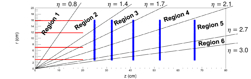
Figure 1: Schematic quadrant view of the pixel detector layout used as a showcase. It covers $|\eta|\;\leq$ 3 in pseudorapidity and shows the segmentation in $\eta$ regions used in this study.

More details on the DELPHES simulation used here are in Appendix A.

3 Real-time Pixel track reconstruction algorithm with vertexing capability

This section presents the PiXTRK algorithm, able to be performed in real-time (i.e. at 40 MHz) and with the determination of the vertex as a “by-product”. The example case is the electron trigger. The used simulation samples for this study are minimum bias data for the background, and single electron gun plus pileup (200) events for the signal. The signal sample consists only of single prompt electrons ($e^{-}$) with a $p_{T}$ range ($p_{T}$ > 10 GeV) corresponding to electron events produced in p-p collisions at 14 TeV c.m energy. The signal windows are defined with the electron sample. For positrons, the $\Delta\phi$ signal windows are directly derived from the ones of the electrons, taking into account their opposite curvature in the transverse plane. Both electrons and positrons have the same $\Delta\eta$ signal windows.

3.1 Real-time Pixel-based track reconstruction algorithm: the strategy

Unlike the tracks reconstructed in real-time (i.e. at 40 MHz) with the outer tracker information in the case of the CMS upgrade for HL-LHC CMS-phase2tracker , the tracks that are based on the pixel information request to be “seeded” i.e. to be searched for within a Region of Interest (RoI) (“L1 clusters/tracks”) that is provided either by the electromagnetic (EM) calorimeter for the electrons, by the muon detectors for the muons, or the outer tracker in the case of the b-tagging. This is due to the very high information rate provided by the extremely high granularity of the microvertex detectors, further increased for the HL-LHC (see Section 6) Therefore the global strategy is based on a seed that can be provided either by the electromagnetic (EM) calorimeter for the electrons, or the muon detectors for the muons, or the outer tracker in the case of the b-tagging.

What is proposed here for the electron case, is easily applicable as well to the muon case. The b-tagging is addressed in Moon_2016 with the specific CMSSW framework; it will be the object of a new paper, because of the increasing importance of the b-tagging at HL-LHC and indeed at future HEP machines.

The pixel-based reconstruction follows the concept of the “PiXTRK” algorithm, first introduced in  Moon_2015 ; Moon_2016 . Its detailed strategy as well as its realistic implementation is developed for the first time in this study.

In order to optimize at best the fast reconstruction efficiency, PiXTRK allows for one missing pixel cluster (e.g. some detector inefficiency) in the pixel track segment. This means, in the detector design considered here, that PiXTRK uses only 3 pixel clusters within 4 selected pixel layers or disks, to reconstruct the pixel tracks in the barrel and/or the endcap or the forward regions of the microvertex. We label it as the “3-out-4 pixel clusters” reconstruction strategy.

The PiXTRK algorithm works in 3 steps:

• Step 1: (RoI) Identifying the pixel clusters in each RoI.

  The first step in pattern recognition for reconstructing the tracks in the microvertex implies identifying the relevant clusters. This procedure is Region of Interest, RoI, based. One RoI is assigned to each L1 e/$\gamma$ candidate that corresponds to an L1 EM trigger cluster with a measured transverse energy, $E_{\textrm{\scriptsize T}}$. The RoI is defined, by linking the L1 EM cluster (EM) to the beam origin, B0, defined by the coordinates ($\phi$ (azimuthal angle)=0, $\eta$ (pseudorapidity)=0, z (beam direction)=0). The RoI is chosen to have an opening of 0.1 rad in $\phi$ and of 3.0 in $|\eta|$. The opening in $|\eta|$ is defined by the present detector design and could be further segmented if needed i.e. if too large for the trigger rate.

  For each RoI, the selected pixel clusters in each layer and/or disks of the pixel detector, are therefore those which are comprised within the $\Delta\phi$ window (Fig. 2):

  $$\centering\Delta\phi=\phi(\textrm{B0},L_{i})-\phi(\textrm{B0},\textrm{EM})<0.1\@add@centering$$ (1)

  The size of the RoI we choose corresponds to a reasonable trigger rate (see Section 5).

  

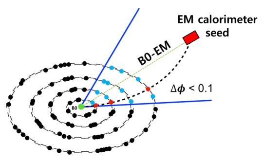
  Figure 2: Step 1 of the PiXTRK algorithm for reconstructing track segments based on pixel only information: definition of the Region of Interest.

• Step 2: (Vector Segment Search) Refined pattern recognition seeded by the L1 EM cluster.

  The next step in the pattern recognition consists in identifying the pixel clusters gathered by pairs, within defined $\Delta\phi$ and $\Delta\eta$ 3$\sigma$ boundaries w.r.t. the segment (B0, EM), as sketched in (Fig. 3). The $\Delta\phi$ and $\Delta\eta$ signal windows are computed as a function of the measured EM E_T. In operation, they will be provided by the analysis of real L1 single electron data allowing the determination of the $\Delta\phi$ and $\Delta\eta$ 3$\sigma$ boundaries.

  For all the pixel clusters selected by the equation 1, for each layer/disk, the algorithm considers each combination of a pair of pixel layers and/or disks in order to form all the possible [$L_{i},L_{j}$] track segments. It then compares the matching in ($\phi$, $\eta$) of each of these [$L_{i},L_{j}$] segments with the segment [B0, EM] joining the beam origin, B0, with the EM cluster. This matching is defined by the following set of boundary conditions:

  $$\centering\Delta\eta_{i,j}=\eta(L_{i},L_{j})-\eta(\textrm{B0},\textrm{EM})<3\sigma\@add@centering$$ (2)

  $$\centering\Delta\phi_{i,j}=\phi(L_{i},L_{j})-\phi(\textrm{B0},\textrm{EM})<3\sigma\@add@centering$$ (3)

  where i, j $=$1…4 or 5 (if disks only) and i $\neq$ j. The pixel cluster in each layer/disk is then only selected if it passes the 3$\sigma$ requirements as specified in Equation 2 and Equation 3.

  

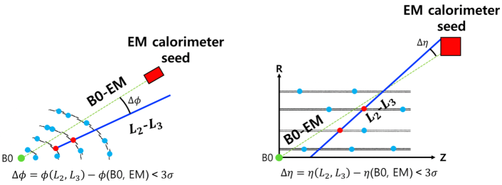
  Figure 3: Step 2 of the PiXTRK algorithm for reconstructing track segments based on pixel only information: refining the coupling in $\eta$ and $\phi$ of the relevant Pixel clusters.

• Step 3: (Bending Correction) The standalone pattern recognition

  This step aims to further reduce the number of combinations with fake clusters. To do so, the algorithm considers all the possible 3-layer combinations with the surviving 2-layer (disk) vector selection in each of the 4 barrel layers or in each of the barrel layers plus disks combinations or in each of the 5 disks combinations, depending on where the RoI is located in $\eta$. The beam origin (B0) is also included. This is sketched in Fig. 4.

  

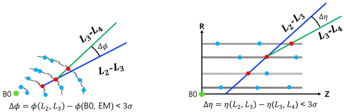
  Figure 4: Step 3 of the PiXTRK algorithm for reconstructing track segments based on pixel only information: The standalone reconstruction is based on 3 out of 4 pixel clusters.

  The pixel clusters must satisfy all the signal windows requirements within 3 standard deviations :

  $$\centering\Delta\eta_{i,j,k}=\eta(L_{i},L_{j})-\eta(L_{j},L_{k})<3\sigma\@add@centering$$ (4)

  $$\centering\Delta\phi_{i,j,k}=\phi(L_{i},L_{j})-\phi(L_{j},L_{k})<3\sigma\@add@centering$$ (5)

  where i, j, k $=$1…4 or 5 (if disks only) and i $\neq$ j $\neq$ k. The pixel cluster in each layer/disk is then only selected if it passes the 3$\sigma$ requirements as specified by Conditions 4 and  5.

  This 3-step procedure thus performs progressively a good pattern recognition. This pattern is then used for a simple track fitting.

The optimized combinations of pixel barrel layers and end-cap disks based on the $\eta$ range they cover in one of the six $\eta$ regions of the microvertex (Fig. 1) are listed in Table 1. This optimization can be used to further decrease the overall data rate when applying the L1 Pixel trigger. It is also a basic tool for the detailed computation of the PiXTRK algorithm explained in Section 3.2.

Region	$\eta$ Range	Pixel Combination
Region 1	$|\eta|<$ 0.8	1-4 layer
Region 2	0.8 $<|\eta|<$ 1.4	1-3 layer, 1 disk
Region 3	1.4 $<|\eta|<$ 1.7	1-2 layer, 1-2 disk
Region 4	1.7 $<|\eta|<$ 2.1	1 layer, 1-3 disk
Region 5	2.1 $<|\eta|<$ 2.7	1-4 disk
Region 6	2.7 $<|\eta|<$ 3.0	2-5 disk

Table 1: The combinations of pixel layers and disks for the different regions in the $\eta$ coverage of the pixel detector.

3.2 Real-time Pixel-based track reconstruction algorithm: the Look-Up-Tables as computing basis

Look-up tables (LUT) are used as a computing basis for efficiently performing the three steps of the PiXTRK algorithm They include the information needed for applying the requirements of Step 2 and Step 3 defined in Section 3.1. These Steps impose constraints on both the $\eta$ and $\phi$ coordinates of the sets of pixels remaining after each of these steps. These constraints (e.g. Conditions 2 and 3 for Step 2 and Conditions 4 and 5 for Step 3) are defined by the size of the 3$\sigma$ windows in $\eta$ and in $\phi$, within which the pixel coordinates must be included. In addition, the size of these windows also varies with the $E_{\textrm{\scriptsize T}}$ of the electron candidate provided by the EM calorimeter at L1.

A detailed study of the dependence in $E_{\textrm{\scriptsize T}}$ of the 3$\sigma$ windows in $\eta$ and $\phi$ for Step 2 and Step 3 is thus performed over the complete acceptance of the pixel detector.

3.2.1 Look-Up Tables describing the dependence in $\eta$

The variation in $\eta$ of the 3$\sigma$ window is studied over the $E_{\textrm{\scriptsize T}}$ range, 10 to 100 GeV, and the full $\eta$ coverage of the pixel detector. This window is found to be constant both in $\eta$ and $\phi$ for Step 2, with a value of $\pm{0.01}$ around zero for the $\Delta\eta$-window. This gives a quick and simple decision about whether or not the considered couple of pixel clusters must be kept at this early decision step.

Three $\Delta\eta$-windows are needed for step 3. They correspond each one to different sectors in $\eta$, namely: $\pm{0.002}$ around zero for $0<\eta<1.7$, $\pm{0.004}$ around zero for $1.7<\eta<2.7$ and $\pm{0.01}$ around zero for $2.7<\eta<3$. If the pixel clusters under consideration do not fulfill the Condition 4 corresponding to their $\eta$ location and as defined here above, they will be discarded without even needing to verify Condition 5. This is a quick and simple cross-check.

Table 2 represents the content of the simple LUT that summarizes the size in $\eta$ of the 3$\sigma$ windows for both Step 2 and Step 3, for applying the Condition 2 to 4 in PiXTRK.

The plots in Fig. 5(a) show the variation as a function of the L1 e/$\gamma$ $E_{\textrm{\scriptsize T}}$ of the size of the 3$\sigma$ window in $\eta$ for three different regions taken as examples: namely for Region 1, Region 4 and Region 6, for Step 2, thus stressing how well this unique value represents all the cases for this step.

For Step 3, the three different values characterizing the size of the 3$\sigma$ window in $\eta$, in the function of L1 e/$\gamma$ $E_{\textrm{\scriptsize T}}$ are presented in Fig. 5(b). The three plots show the variation in function of L1 e/$\gamma$ $E_{\textrm{\scriptsize T}}$ of the size of the 3$\sigma$ window in $\eta$ for Region 1, Region 3, and Region 5 respectively.

Step 2	$\eta$ Region 1-6	3$\sigma$ $\Delta\eta_{i,j}$ = 0.01
Step 3	$\eta$ Region 1-2	3$\sigma$ $\Delta\eta_{i,j,k}$ = 0.002
	$\eta$ Region 3	3$\sigma$ $\Delta\eta_{i,j,k}$ = 0.004
	$\eta$ Region 4-6	3$\sigma$ $\Delta\eta_{i,j,k}$ = 0.01

Table 2: $\eta$-LUT table providing the 3$\sigma$ window size in $|\eta|$ to be applied for Step 2 and Step 3 of the PiXTRK algorithm.

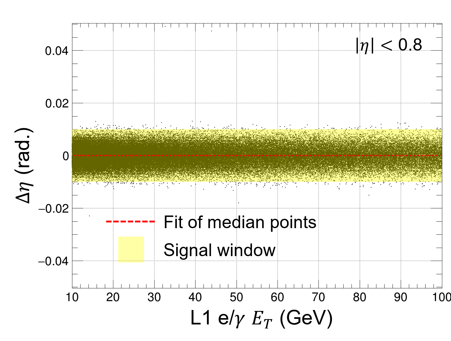
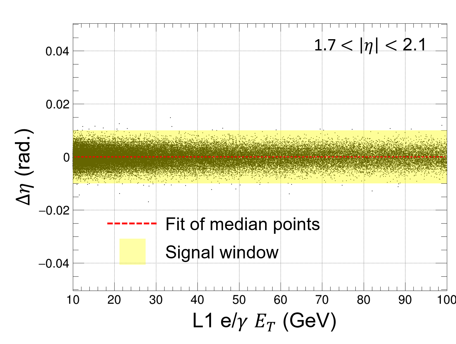
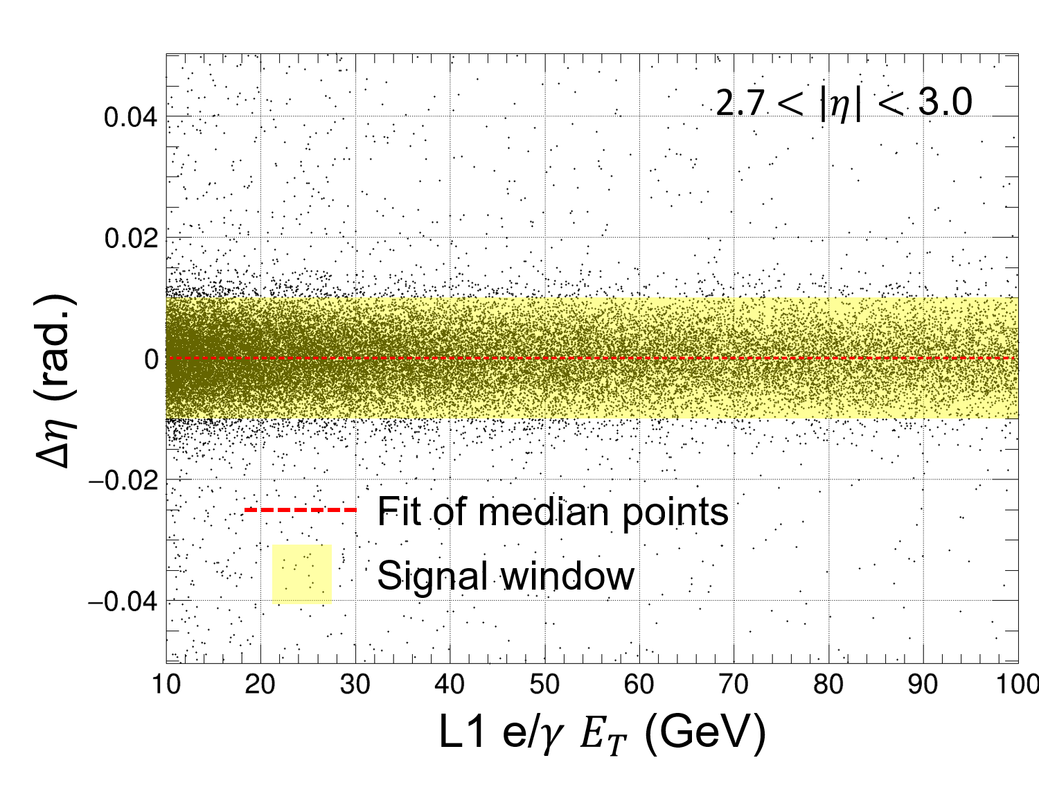
(a) step 2

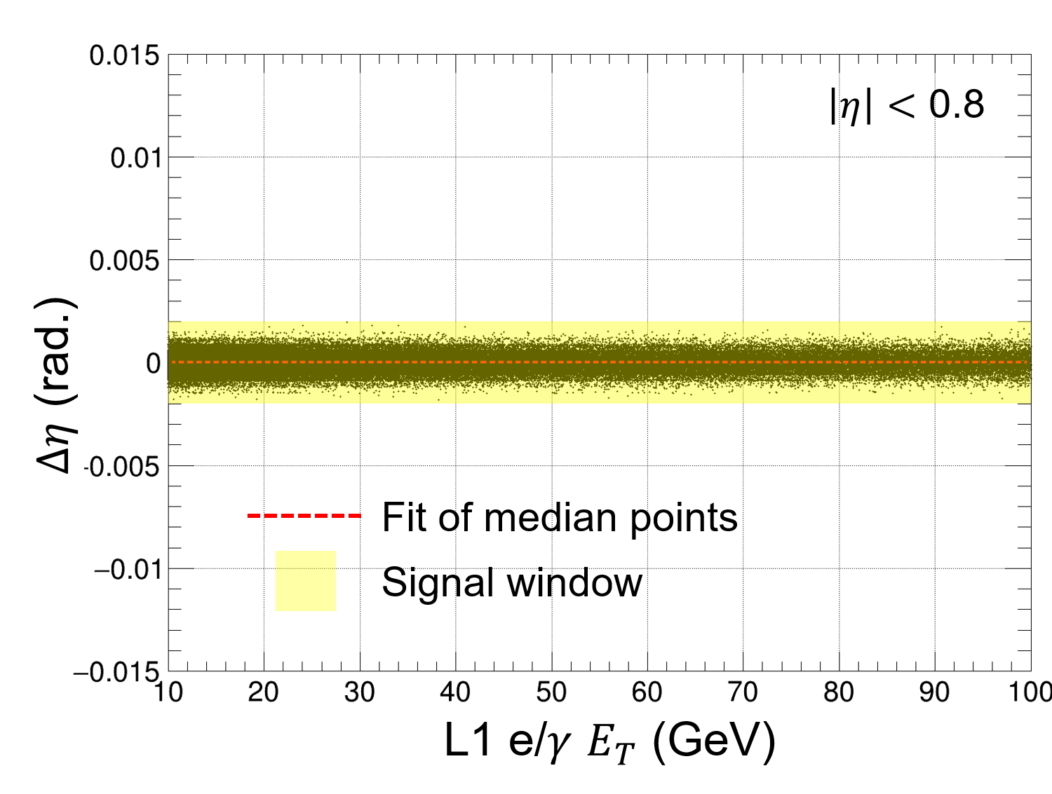
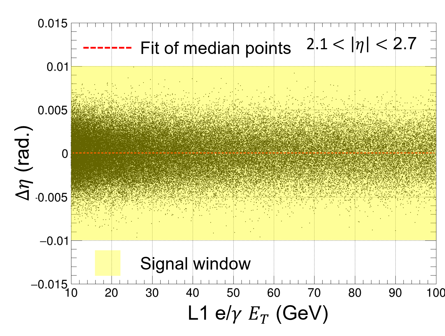
(b) step 3

Figure 5: (a) Step 2: Variation, in function of the L1 e/$\gamma$ $E_{\textrm{\scriptsize T}}$, of the size of the 3$\sigma$ window in $\eta$ (yellow band) and of the residuals in $\eta$ (black points) from Equation 2, for central barrel (left), endcap (middle) and forward (right). (b) Step 3: Equivalent distributions as above, but for step 3, thus corresponding to Equation 4. These curves correspond to the electron case. Both electrons and positrons have the same $\Delta\eta$ distributions.

3.2.2 Look-Up Tables describing the dependence in $\phi$

The variation of the size of the 3$\sigma$ windows in azimuthal angle, over the full $E_{\textrm{\scriptsize T}}$ range is more complex for both Step 2 and Step 3 of the PiXTRK algorithm.

This is so because the typical dependence in $E_{\textrm{\scriptsize T}}$ of the upper and lower bounds of these 3$\sigma$ windows, for Step 2 and Step 3, is not at all constant; it varies quite fast especially in the low $E_{\textrm{\scriptsize T}}$ range between 10 and 20 GeV and in different ways over the full $\eta$ range. Moreover, in Step 2, the $\Delta\phi$ resolution is dominated by the calorimeter granularity and the distance of the calorimeter to the beam axis. The chosen calorimeter design, in this showcase study, is made of a barrel calorimeter with a coarser granularity but a shorter distance (by about a factor of 2) from the beam axis than the endcap calorimeter. This is reflected in the Step 2 results in Fig. 6 as well as in Appendix B.1. Step 3 instead corresponds to the “standalone”-based track reconstruction, thus the $\Delta\phi$ resolution is dominated by the pixel high granularity (see results in Appendix B and Fig. 6). It is typically here, a factor of 10 better.

The variation of the size of the $\Delta\phi$-windows has been carefully studied. The results summarized here below show an impressive agreement between the DELPHES results and those with a full simulation .

• The $\Delta\phi$-window LUT for PiXTRK Step 2

  The variation of the 3$\sigma$ windows in $\phi$ boundaries are studied as a function of L1 e/$\gamma$ $E_{\textrm{\scriptsize T}}$ and in all the 6 regions in $\eta$ as defined in Table 1.

  As a result, a LUT is defined with compressed values, reducing the dimensions of this Table, but still preserving a high precision. It is made of 20 steps in transverse energy ($E_{\textrm{\scriptsize T}}$), where the first 10 steps of 1 GeV each represents the variation from 10 to 20 GeV, then by steps of 2 GeV from 20 to 30 GeV and steps of 5 GeV from 30 to 50 GeV. The value at 50 GeV is kept as a constant step, for $E_{\textrm{\scriptsize T}}$ larger than 50 GeV. The other parameter to include in this LUT represents the three combinatorial possibilities between the 4 barrel layers and the 5 end cap disks, over the full $\eta$ coverage. It can be split into 4 sectors, where the first one extends from 0 to 2.1 in $\eta$ (thus merging in one sector the 3 first regions) and the other sectors correspond each to regions 4, 5, and 6 as defined in Table 1. The total number of $\Delta\phi$ values included in this $\Delta\phi$-LUT is 160 and their detailed values are in Appendix B.1. Note that, unlike the $\Delta\eta$-LUT, the $\Delta\phi$-LUT does not define the size of the 3$\sigma$ window in $\Delta\phi$ by just one $\Delta$-like value centered around 0, but indeed by two values which correspond to the lower and upper boundaries for each L1 $E_{\textrm{\scriptsize T}}$ of the defined windows.

  One may note that the $E_{\textrm{\scriptsize T}}$ dependence of the $\Delta\phi$-windows is sharper in the first 3 regions in $\eta$ (i.e Regions 1, 2 and 3) than for the 3 other Regions 4, 5 and 6. Indeed the curve flattens when corresponding to larger $\eta$ regions and thus, especially, when getting to Region 6.

  As examples we show some plots of the 3$\sigma$ windows in Fig. 6; they correspond, from left to right, to Region 1, Region 4, and Region 5, respectively.

  

  

  

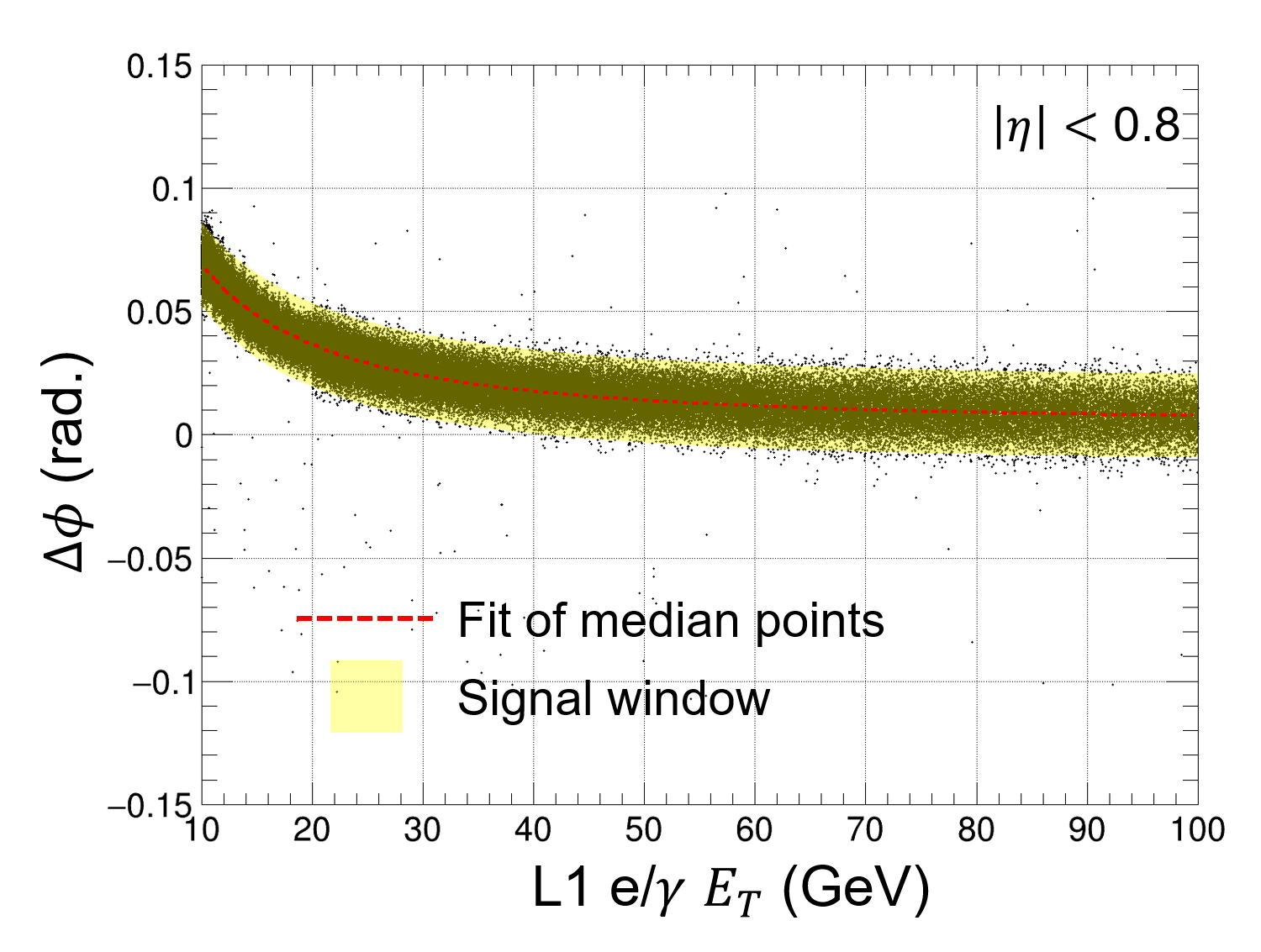
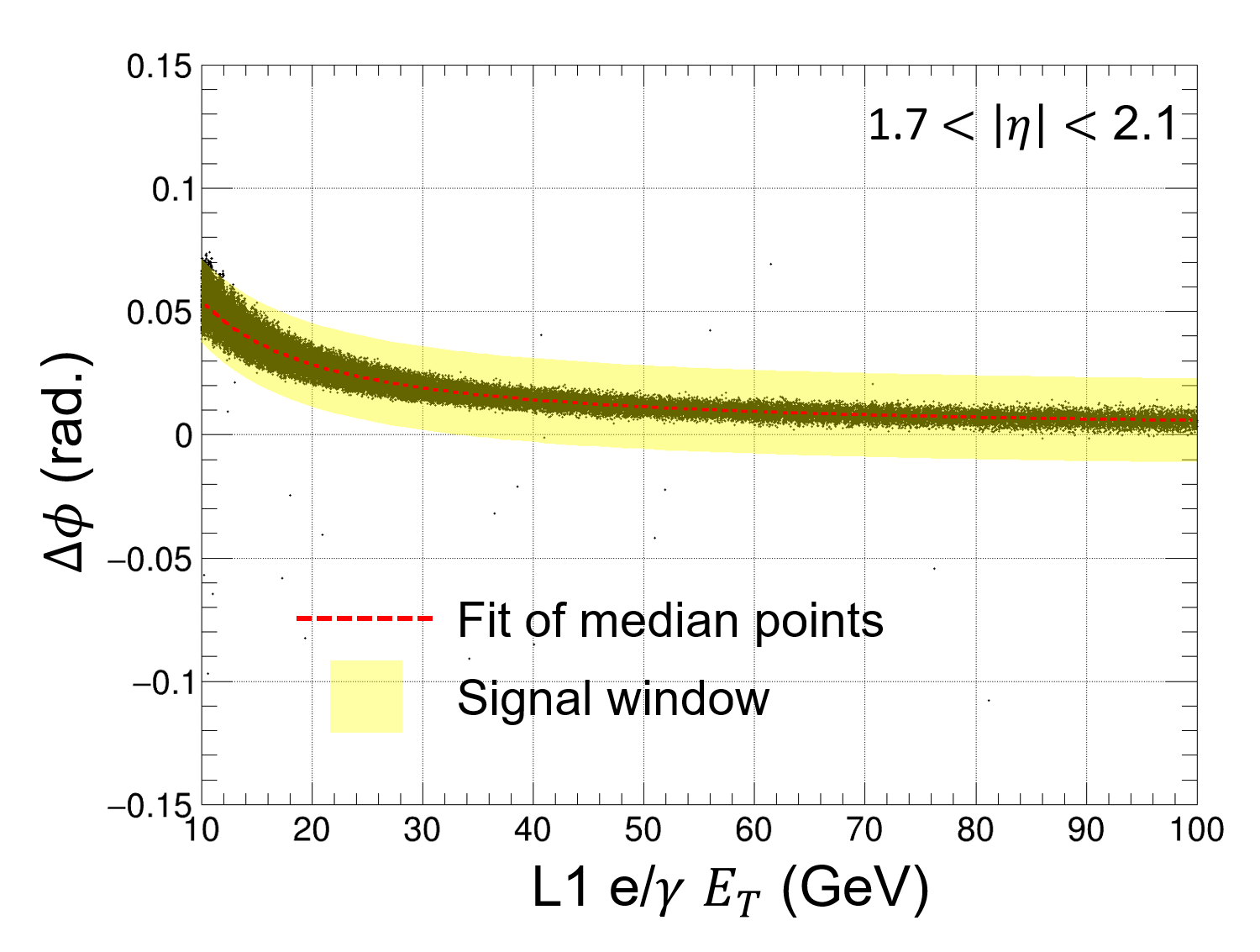
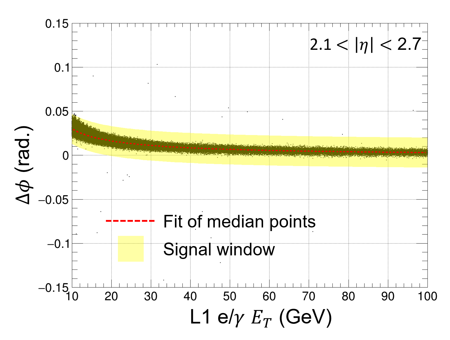
  (a) Step 2

  

  

  

  (b) Step 3

  Figure 6: (a) Step 2: Variation, in the function of the L1 e/$\gamma$ $E_{\textrm{\scriptsize T}}$, of the size of the 3$\sigma$ window in $\Delta\phi$ (yellow band) and of the residuals in $\phi$ (black points) from Equation 3, for central barrel (left), endcap (middle) and forward (right). (b) Step 3: Equivalent distributions as above, but for step 3, thus corresponding to Equation 5. These curves correspond to the electron case. The corresponding $\Delta\phi$ distributions for the positrons are symmetrical w.r.t. $\Delta\phi$ = 0 axis, to the ones of the electrons presented in this Figure.

  At this stage in Step 2, the PiXTRK algorithm cross-checks Condition 3 only for the pixel clusters satisfying Condition 2. To do so, it looks for the specific $\Delta\phi$ window size as provided in Step 2 $\Delta\phi$-LUT, that corresponds to the $\Delta\eta$ region in the detector and the transverse energy of the electron candidate which is measured by the EM calorimeter at L1. Only the pixel clusters satisfying Condition 3 will go to Step 3.

• The $\Delta\phi$-window LUT for PiXTRK Step 3

  This step corresponds to the standalone (track bending) part of PiXTRK, defined with all the combinations between 3 pixel clusters in different layers and/or disks, remaining after the 2 first selection steps.

  The study of the $\Delta\phi$-window evolution with the $\eta$ and $\phi$ positions of the remaining pixel clusters and on the $E_{\textrm{\scriptsize T}}$ of the electron candidate shows that higher precision is required on those parameters. Indeed, the corresponding $\Delta\phi$-LUT contains, in this case, 2400 values, namely: 400 boundary values for each of the six regions in $\eta$, to start with.

  The goal is to compress this large data sample without jeopardizing the precision. This is successfully achieved by combining in each region the ranges in transverse energy with the same boundaries. An overall reduction factor of almost 5 is obtained, leading to a total of 526 values to be reported in this LUT.

  This study gives a precision on Conditions 3 and 5 of 1 mrad in $\Delta\phi$. The details of the content of these LUTs can be found in Appendix B.2.

  Applying Condition 5 to the remaining pixel clusters after passing Conditions 1 to 4, is the last selection step of the PiXTRK algorithm.

3.3 Vertexing performance in z-direction with pixel-based information

The vertexing capability i.e. the capability to reconstruct vertex in the collision points is indeed a fundamental role of the microvertex detectors installed in the closest neighbourhood of the beam pipe. The microvertex information is used for vertexing the collision point, in the z-direction, at the High-Level Trigger (HLT) which is the final stage of the triggering system in both the ATLAS and CMS experiments for instance.

The feasibility studies for using the pixel cluster information in real-time i.e. at 40 MHz have already been performed both for the electron trigger and the b-tagging case and reported in Moon_2015 ; Moon_2016 . In the b-tagging case Moon_2016 the seed is provided by the L1 track defined with the outer tracker CMS-phase2tracker ; we then look for the pixel track segment (defined by 2 pixel clusters) compatible with the L1 track reconstructed by the L1 track trigger system CMS-phase2L1TDR .

As this paper focuses on the electron case, we thus stress here the potential of the pixel detector for a high precision reconstruction of the z-vertex for the electron trigger(s); this would be similar for the muon trigger(s), as the bremsstrahlung is in the transverse plane (see for instance CMS-HLTPhase2TDR ). This trigger, as explained above, is provided by the pixel detector plus the EM calorimeter: the seed element, namely the L1 e/$\gamma$ reconstructed object, is provided by the L1 EM calorimeter system.

The data samples we use are single electron gun events produced at 14 TeV with 200 superimposed pileup. The reconstructed z-vertex position is obtained as a direct outcome of the PiXTRK as described in Section 3.1 and Moon_2015 . The straight line joining the two most distant pixel clusters out of the three used by PiXTRK to reconstruct the pixel track segment (i.e. the cluster in the innermost and the one in the outermost layer or disk), is further extended till the beam axis. The intercepting “$z_{vtx}$” point, fits quite closely with the z-coordinate of the true vertex.

In order to verify the validity of this approach and to evaluate its precision, we study the difference between the reconstructed z-vertex position along the beam axis, $z_{vtx}$, and the z-vertex position of the “true” primary vertex as given at the generator level (gen-level), in the six different $\eta$ regions as defined in Table 1.
Figure 7 gives the resolution in the determination of the z-vertex position as given by this simple vertex determination method. The resolution of each distribution is defined by a standard deviation from a fitted Gaussian function. Excellent 1$\sigma$ resolutions are obtained: in the barrel with 20$\mu$m resolution for $\eta$ up to 0.8 and with 30$\mu$m for 0.8 <$\eta$< 1.4) as well as in the intermediate region 1.4 < $\eta$ < 2.1, with 60$\mu$m. The resolution increases by about a factor 4 in the end-cap (2.1 < $\eta$ < 2.7) and by a factor 6 in the very forward region ($\eta$ > 2.7 reaching a maximum value of about 360$\mu$m.
The 1$\sigma$ resolution of this vertex reconstruction method for $\eta$ < 2.5, is shown in Fig. 8. A resolution of 46.4$\mu$m, on average, is obtained over this overall $\eta$ range. It should be noted here, that because the single electrons sample includes a large fraction of central electrons, this average estimate is biased towards values corresponding to $\eta$ < 1.4.
For completion, these results can be compared to the vertex resolution of 37$\mu$m in the central part ($\eta$ < 1.5), with the same method applied to the b-tagging case Moon_2016 using top pair events and improving by more than an order of magnitude the resolution with the outer tracker only.

(a)

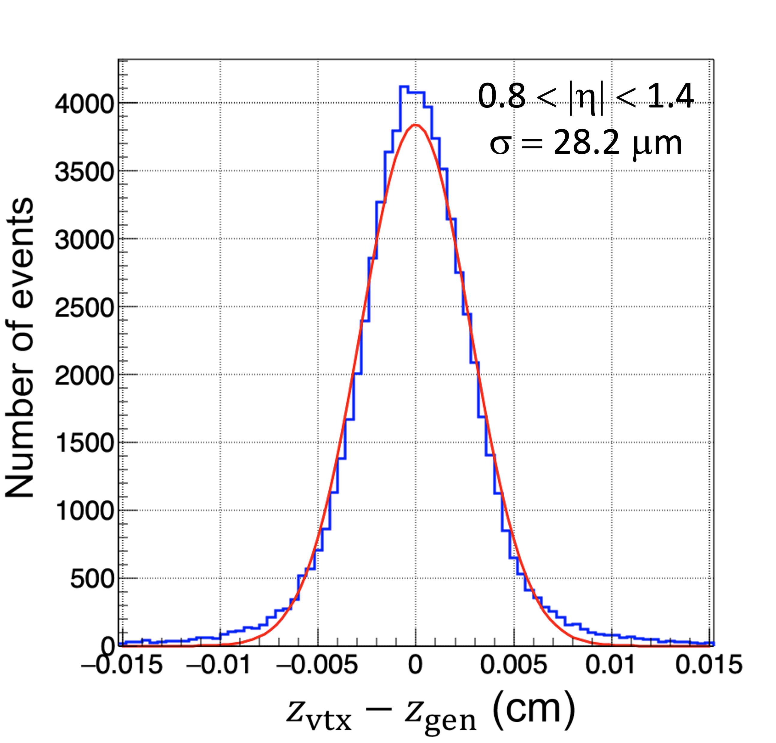
(b)

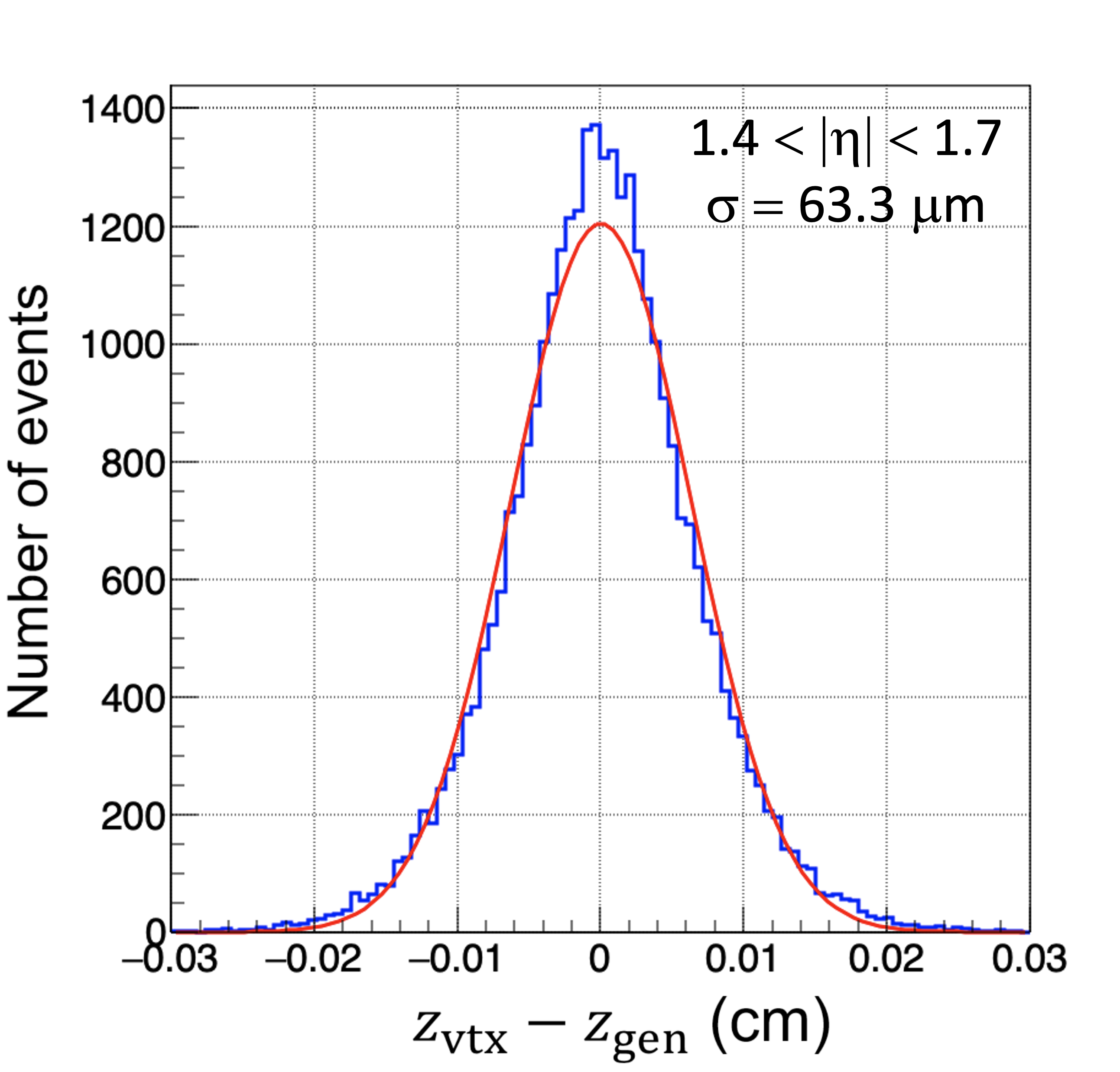
(c)

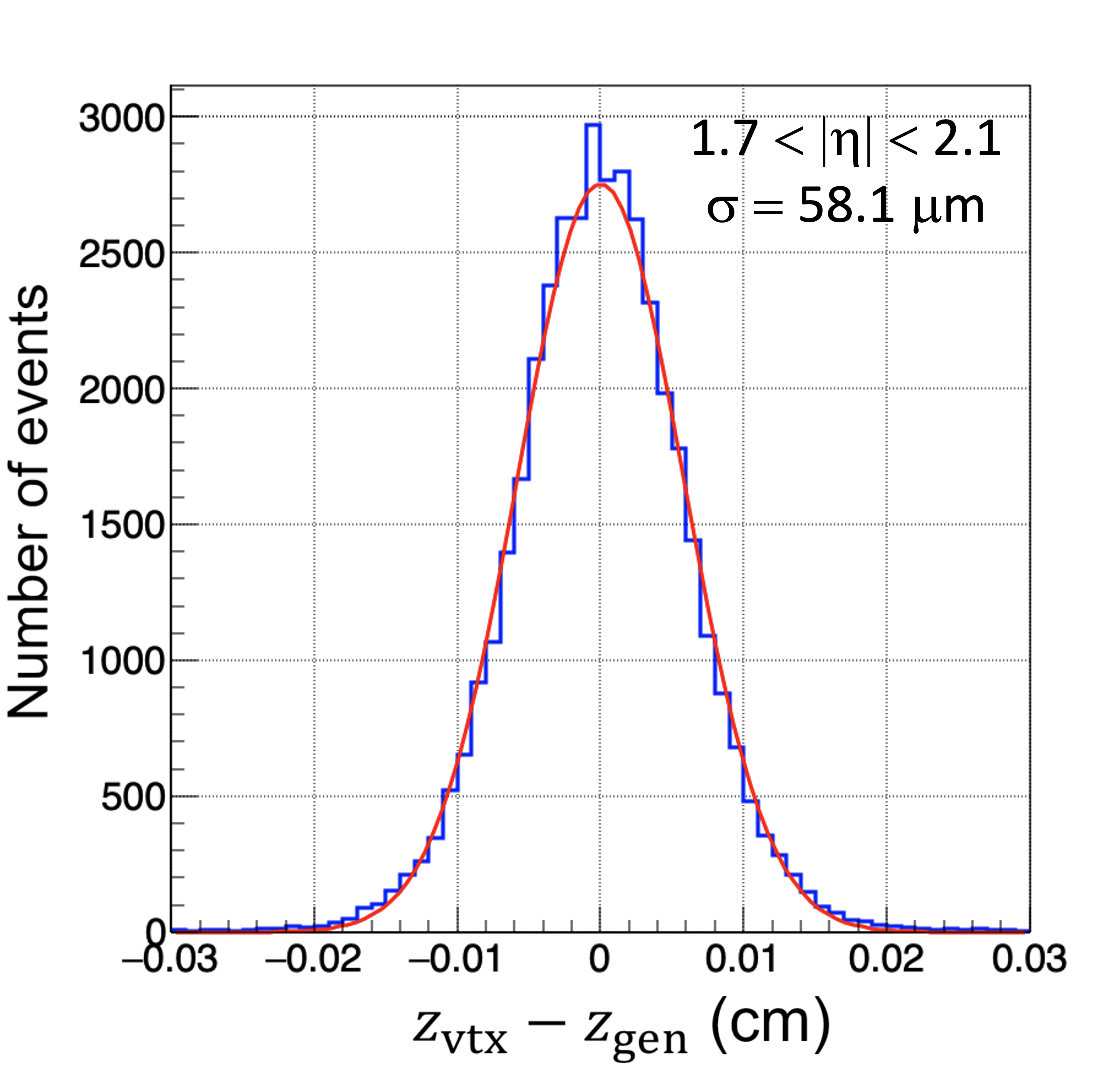
(d)

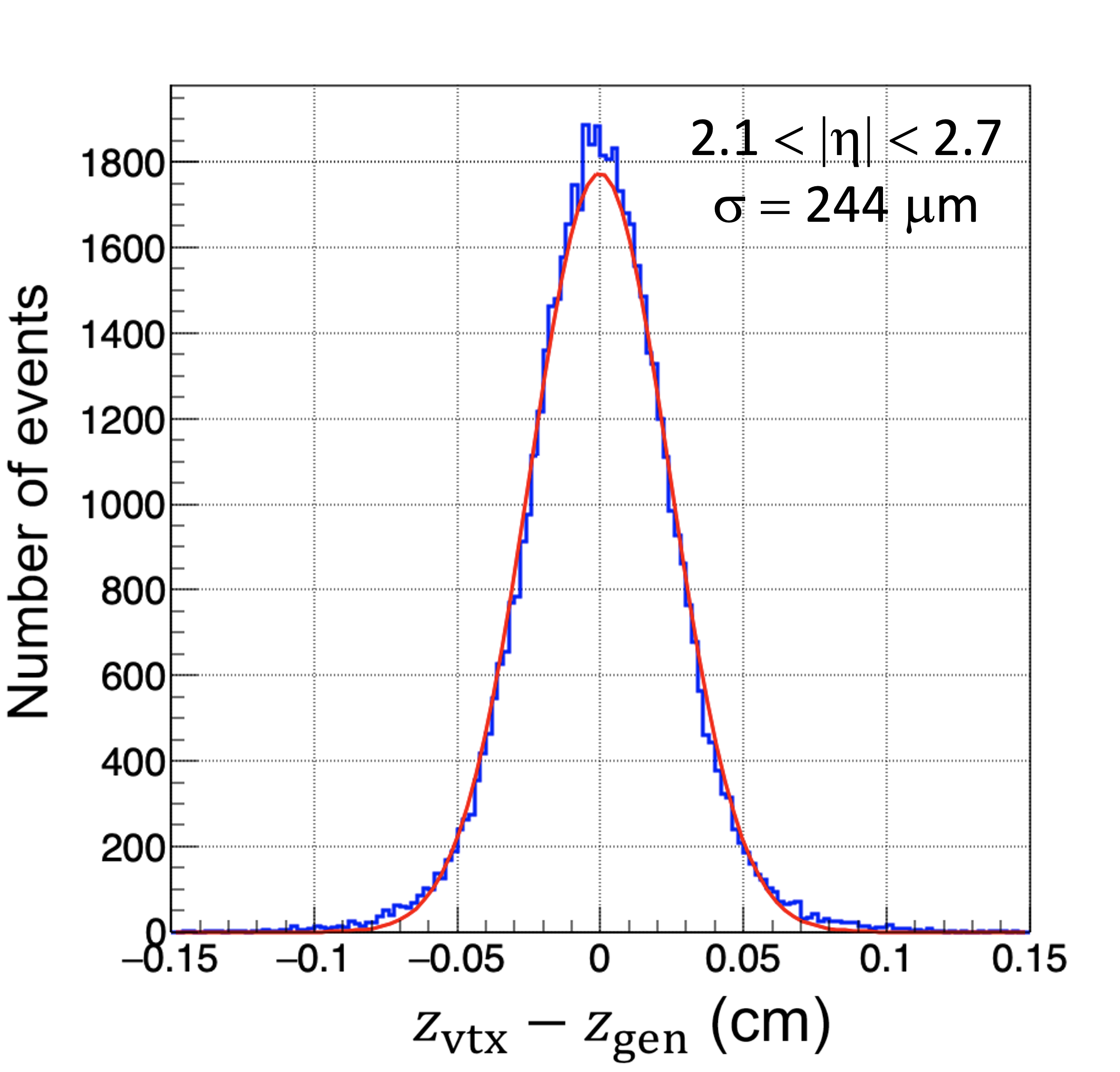
(e)

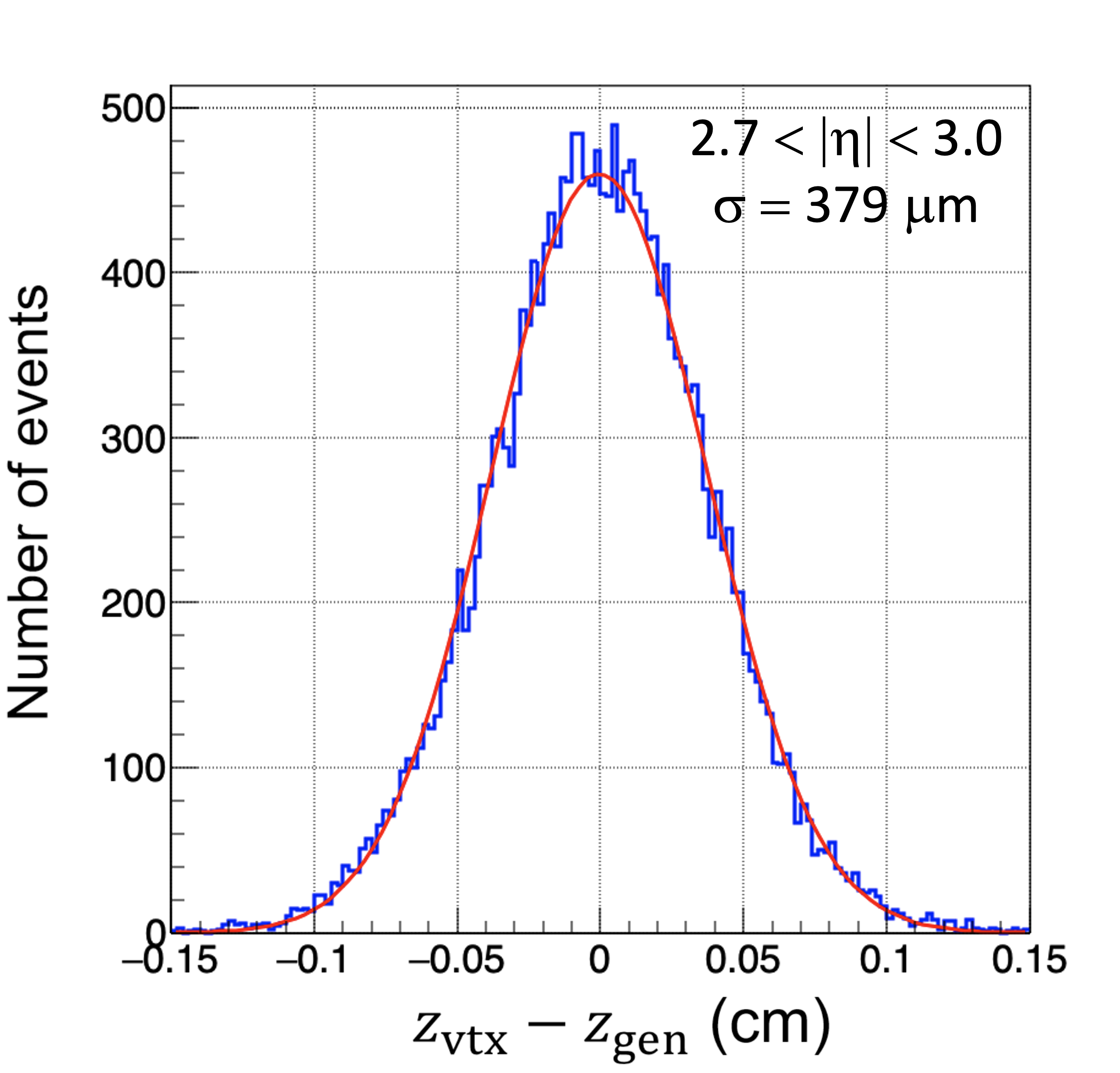
(f)

Figure 7: Distributions of the distance between the vertex of the L1 e/$\gamma$ object determined by the simple method described above and the true vertex at generator level, in different $\eta$ regions. The fit performed with a Gaussian function is shown in red. The standard deviation ($\sigma$) of the fitted Gaussian function represents the resolution of each distribution.

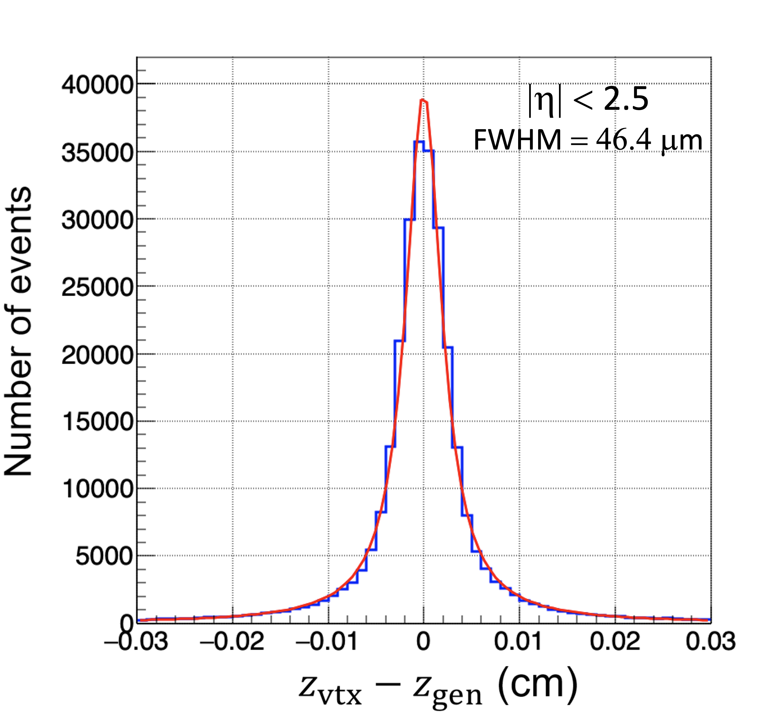
Figure 8: Distribution of the distance between the vertex of the L1 e/$\gamma$ object determined by the simple method described above and the true vertex at generator level, over the overall range in $\eta<2.5$. The fit with the Cauchy distribution function is shown in red.

4 Track Isolation based on the Pixel Detector Only Information

The track isolation using only the pixel-based tracks is implemented to further improve the performances of the PiXTRK algorithm, for the single electron trigger as a showcase. The isolation consists of counting the number of reconstructed pixel-based tracks included in an isolation cone. It follows the main steps here below:

• Reconstruction of the leading electron track and definition of the isolation cone

• Reconstruction of all the pixel-based tracks within the isolation cone.

  1) Look for all the pixel clusters within the isolation cone

  2) Reconstructing the track segments.

  3) Reconstructing the pixel tracks within the cone

  4) Measuring the azimuthal $\phi$ curvature

• Computation of the pixel-based tracks $p_{\textrm{\scriptsize T}}$ and application to pixel track isolation

• Estimate of the electron track isolation

4.1 Reconstruction of the leading electron track and definition of the isolation cone

The pixel-based track reconstruction of the considered electron, labeled as “leading or L1 electron track” is performed with PixTRK (Section 3). Its z-vertex ($z_{\textrm{\scriptsize vtx}}$) position is defined as in (Section 3.3). A cone with a typical aperture of 0.2 to 0.4, is defined around the leading electron track, originating from the z-vertex position ($z_{\textrm{\scriptsize vtx}}$), as sketched in Fig. 9.

4.2 Reconstruction of all the pixel-based tracks within the isolation cone

4.2.1 Look for all the pixel clusters within the isolation cone

Each pixel cluster position within this cone is defined with its $\phi$, $\eta$ coordinates, and corresponding z-vertex position. The $\eta$ pixel cluster is evaluated assuming that the particle originated at the electron z vertex. The coordinates in $\phi$, $\eta$ of the ith-cluster, for this cluster to be included in the cone, must verify that $\Delta R$ as defined in Equation 6 is within the chosen cone aperture.

$$\centering\Delta R=\sqrt{(\phi_{\textrm{\scriptsize L1 electron}}-\phi_{\textrm{\scriptsize pixel cluster}}^{i\textrm{\scriptsize th}})^{2}+(\eta_{\textrm{\scriptsize L1 electron}}-\eta_{\textrm{\scriptsize pixel cluster}}^{i\textrm{\scriptsize th}})^{2}}\@add@centering$$ (6)

where $\phi_{\textrm{\scriptsize L1 electron}}$ and $\eta_{\textrm{\scriptsize L1 electron}}$ are the azimuthal angle and the pseudorapidity angle of the L1 electron track while $\phi_{\textrm{\scriptsize pixel cluster}}^{i\textrm{\scriptsize th}}$ and $\eta_{\textrm{\scriptsize pixel cluster}}^{i\textrm{\scriptsize th}}$ are the azimuthal angle and the pseudorapidity angle of the $i$th-cluster.

Figure  9 illustrates the tracks that might be fully included or just crossing the cone space (pileup tracks for instance).

4.2.2 Reconstructing the track segments

Pixel track segments combining two pixel clusters within this cone are formed. Their intercept with the z-beam axis, defines the corresponding $z^{\prime}$ value (Fig. 9).
The $z^{\prime}$ value is compared to the z-vertex ($z_{\textrm{\scriptsize vtx}}$) as defined above. $\Delta z$ defined as the distance along the z-axis between the track segment joining these two pixel clusters and the $z_{\textrm{\scriptsize vtx}}$ from the leading electron, which must satisfy Equation 7.

$$\centering\Delta z=|z_{\textrm{\scriptsize vtx}}-z^{\prime}|<3\sigma\@add@centering$$ (7)

If Equation 7 is not satisfied the combination of corresponding two pixel clusters is disregarded.

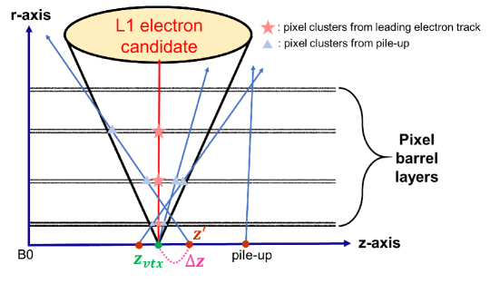
Figure 9: A schematic of the cone from the $z_{\textrm{\scriptsize vtx}}$ to the L1 electron pixel-based track to select pixel clusters satisfying $\Delta R<$0.3. It illustrates how additional pixel track segments can be fully included or just crossed in the cone space. Here the $r$-axis is defined as $r=\sqrt{x^{2}+y^{2}}$, where $x$ and $y$ axes are perpendicular to the z-axis (i.e. in the transverse plane).

In the considered pixel design, four possible combinations of layers or disks have to be taken into account. As an example, the possible combinations of two pixel clusters from different pixel barrel layers for measuring $\Delta z$ are shown in Table 3, for the detector region defined by $|\eta|<$ 0.8.

Pixel barrel layers	Combinations of two pixel clusters for measuring $\Delta z$
1st, 2nd, 3rd layer	1st-2nd layer	1st-3rd layer	2nd-3rd layer
1st, 2nd, 4th layer	1st-2nd layer	1st-4th layer	2nd-4th layer
1st, 3rd, 4th layer	1st-3rd layer	1st-4th layer	3rd-4th layer
2nd, 3rd, 4th layer	2nd-3rd layer	2nd-4th layer	3rd-4th layer

Table 3: The combination of pixel barrel layers for measuring $\Delta z$ in the region: $|\eta|<$ 0.8.

4.2.3 Reconstructing the pixel tracks within the cone

A third pixel cluster must be found that combines the two first pixel clusters selected above. To do so, the pseudorapidity angle difference among the three pixel clusters as shown in Fig. 10 (a) is measured. It can be expressed as (8):

$$\Delta\eta_{\textrm{\scriptsize pix}}=\eta\left(L_{i},L_{j}\right)-\eta\left(L_{j},L_{k}\right)<3\sigma$$ (8)

where i, j, k $=$1…4 or 5 (if disks only) and i $\neq$ j $\neq$ k.

The pixel track segment is made by the connection between the leading electron track vertex and the selected pixel cluster (Fig. 10 (b)). The reconstructed electron vertex is used to calculate the pseudorapidity angle. The angle difference is calculated according to (9):

$$^{ji}\Delta\eta_{\textrm{\scriptsize vtx}}=\eta\left(z_{\textrm{\scriptsize vtx}},L_{i}\right)-\eta\left(z_{\textrm{\scriptsize vtx}},L_{j}\right)<3\sigma$$ (9)

where i, j $=$1…4 or 5 (if disks only) and i $\neq$ j. Based on the measured pseudorapidity angle difference, the pixel clusters generated from pileup can be excluded from the pixel track reconstruction.

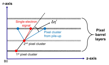
(a)

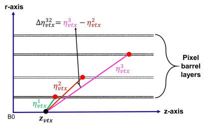
(b)

Figure 10: Examples of reconstructing pixel track segment (a) using three pixel clusters and (b) using the L1 electron PiXTRK reconstructed vertex and pixel clusters. The example here is with layers 1, 2, and 3 starting from the innermost layer.

The duplicated pixel tracks are removed by indexing each reconstructed track.

4.2.4 Measuring the azimuthal $\phi$ curvature

The $\Delta\phi$ angle difference in the transverse plane (see Fig. 11). is expressed as follows:

$$\Delta\phi\;\textrm{difference}=[\phi(\textrm{B0},L_{i})-\phi(L_{i},L_{j})]-[\phi(L_{i},L_{j})-\phi(L_{j},L_{k})]<3\sigma$$ (10)

where i, j, k $=$1…4 or 5 (if disks only) and i $\neq$ j $\neq$ k. The $\Delta\phi$ difference of the pixel track segments will be smaller when the corresponding track $p_{\textrm{\scriptsize T}}$ is higher.

This is the last stage to reject fake tracks coming from combinatorial backgrounds.

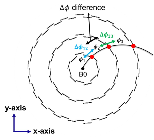
Figure 11: Schematic transverse view of the $\Delta\phi$ difference for the barrel region.

4.3 Computation of the pixel-based tracks $p_{\textrm{\scriptsize T}}$

After reconstructing the pixel-based tracks, additional information is provided by this detector, namely the $p_{\textrm{\scriptsize T}}$ of the tracks. A new method is developed to compute this parameter. It is based on the well known formula:

$$\centering p_{\textrm{\scriptsize T}}=0.003*B*R_{track}\@add@centering$$ (11)

where $B$ is the magnitude of the magnetic field in which the tracker is merged, and $R_{track}$ (in cm) is the radius of the circle made with B0 and two of the pixel clusters relative to the reconstructed pixel track in the transverse plane (see Appendix C for details).
The track $p_{\textrm{\scriptsize T}}$ is computed using a DELPHES sample of single electrons with $p_{\textrm{\scriptsize T}}$ ranging from 0 to 100 GeV and no pileup included. The $p_{\textrm{\scriptsize T}}$ resolution is defined by:

$$\frac{(\textrm{reconstructed track}\>p_{\textrm{\scriptsize T}}-\textrm{gen-level track}\>p_{\textrm{\scriptsize T}})}{\textrm{gen-level track}\>p_{\textrm{\scriptsize T}}}$$ (12)

where the gen-level quantity is provided by the simulated single electron tracks.
The results as a function of the gen-level $p_{\textrm{\scriptsize T}}$, are shown in Fig. 12. Note that this is a pure electron sample i.e. with no PU. For example, the top plot shows the resolution for tracks with the two clusters in the central barrel (Layers 1 and 4). The bottom plot corresponds to tracks in the endcap-forward region with the two clusters in Disk 2 and Disk 5. The tracks with only $p_{\textrm{\scriptsize T}}$ between 0.5 and 10 GeV are plotted, as rather low $p_{\textrm{\scriptsize T}}$ tracks are relevant for computing the track isolation.
In the central barrel, the resolution is smaller than 1% up to 3 GeV $p_{\textrm{\scriptsize T}}$ and smaller than 3% up to 10 GeV $p_{\textrm{\scriptsize T}}$. For most of the central tracks the $p_{\textrm{\scriptsize T}}$ resolution remains within 10% even for tracks up to 30 GeV. For tracks in the endcap and forward regions, the $p_{\textrm{\scriptsize T}}$ resolution increases to 5% up to 10 GeV and stays around at most 20% for tracks larger than 10-15 GeV $p_{\textrm{\scriptsize T}}$.

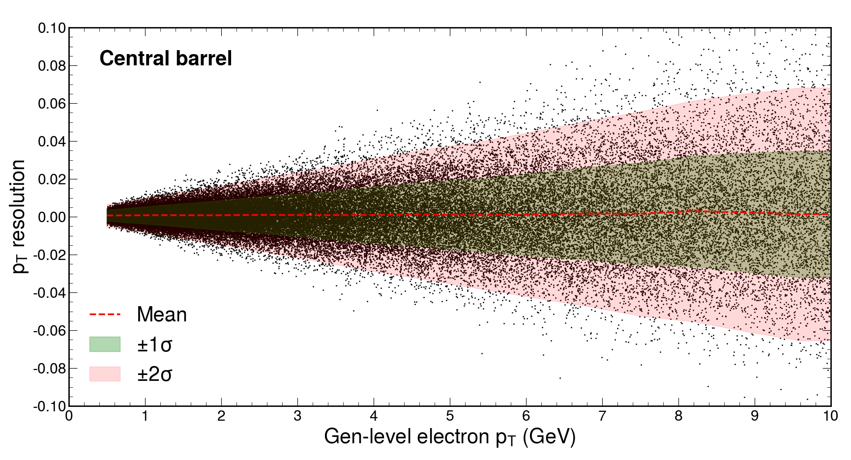
(a)

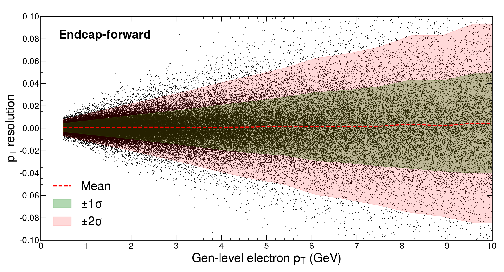
(b)

Figure 12: The resolution of the reconstructed track $p_{\textrm{\scriptsize T}}$ as defined in Equation 12, in function of the gen-level track $p_{\textrm{\scriptsize T}}$ is shown on the top plot for tracks in the central barrel and on the bottom plot for tracks in the endcap region, based on a pure electron sample thus with no PU.

4.4 Estimate of the electron track isolation

If the number of pixel tracks is zero or one in the isolation cone, the L1 electron track is isolated. If the isolation cone contains n >1 pixel tracks, with $p_{\textrm{\scriptsize T}}^{1}$ to $p_{\textrm{\scriptsize T}}^{n}$ in increasing order, the pixel track isolation value is calculated as the ratio of two linear $p_{\textrm{\scriptsize T}}$ sum shown in Equation 13.

$$\centering\textrm{Pixel Track Isolation}=\frac{\sum_{i=1}^{n-1}p_{\textrm{\scriptsize T}}^{i}}{\sum_{i=1}^{n}p_{\textrm{\scriptsize T}}^{i}}\@add@centering$$ (13)

The numerator is a linear sum of all the reconstructed pixel tracks $p_{\textrm{\scriptsize T}}$ except the one of the leading track, i.e. the electron track. The denominator is a linear sum of all the pixel tracks $p_{\textrm{\scriptsize T}}$. A minimum $p_{\textrm{\scriptsize T}}$ of 0.5 GeV for all the reconstructed tracks in the cone is assumed, except for the one of the electron track, which is at least of 10 GeV.

In order to validate the procedure for determining the pixel track isolation, the isolation distributions of the electron (signal) events are compared with the background events. A sample of single electrons with 200 pileup is used for the signal events while a minimum bias sample is used for the background.

Since the pixel track isolation algorithm depends on the number of tracks inside of the isolation cone, the simulation must well reproduce the content of the overall track including the soft tracks. The additional tracks from bremsstrahlung have thus to be included in the signal events of the DELPHES simulation, as DELPHES does not include this physics process.

Figure 13 shows the isolation distributions of the signal events (in blue) and the overall background, i.e. minimum bias plus bremsstrahlung events, (in red), in each $\eta$ range, and for electrons with $E_{\textrm{\scriptsize T}}$ larger than 20 GeV.

The distribution in a number of events as a function of the pixel track isolation value, for the signal (in blue) and for the background (in red), are normalized to one. The first bin corresponds to a pixel track isolation equal to zero, i.e. no additional track with at least 0.5 GeV in the isolation cone.

The pixel track isolation for the electron tracks depends on the $\eta$ range (Fig. 13). Additional tracks can be produced by bremsstrahlung due to the higher material budget in the endcap regions. These tracks contribute to a fair fraction of the single electron signal events in the forward region (2.1 $<|\eta|<$ 3.0) thus increasing the value of the pixel track isolation. As a result, the background rejection is lowered in the endcaps.

(a) Region 1

(b) Region 2

(c) Region 3

(d) Region 4

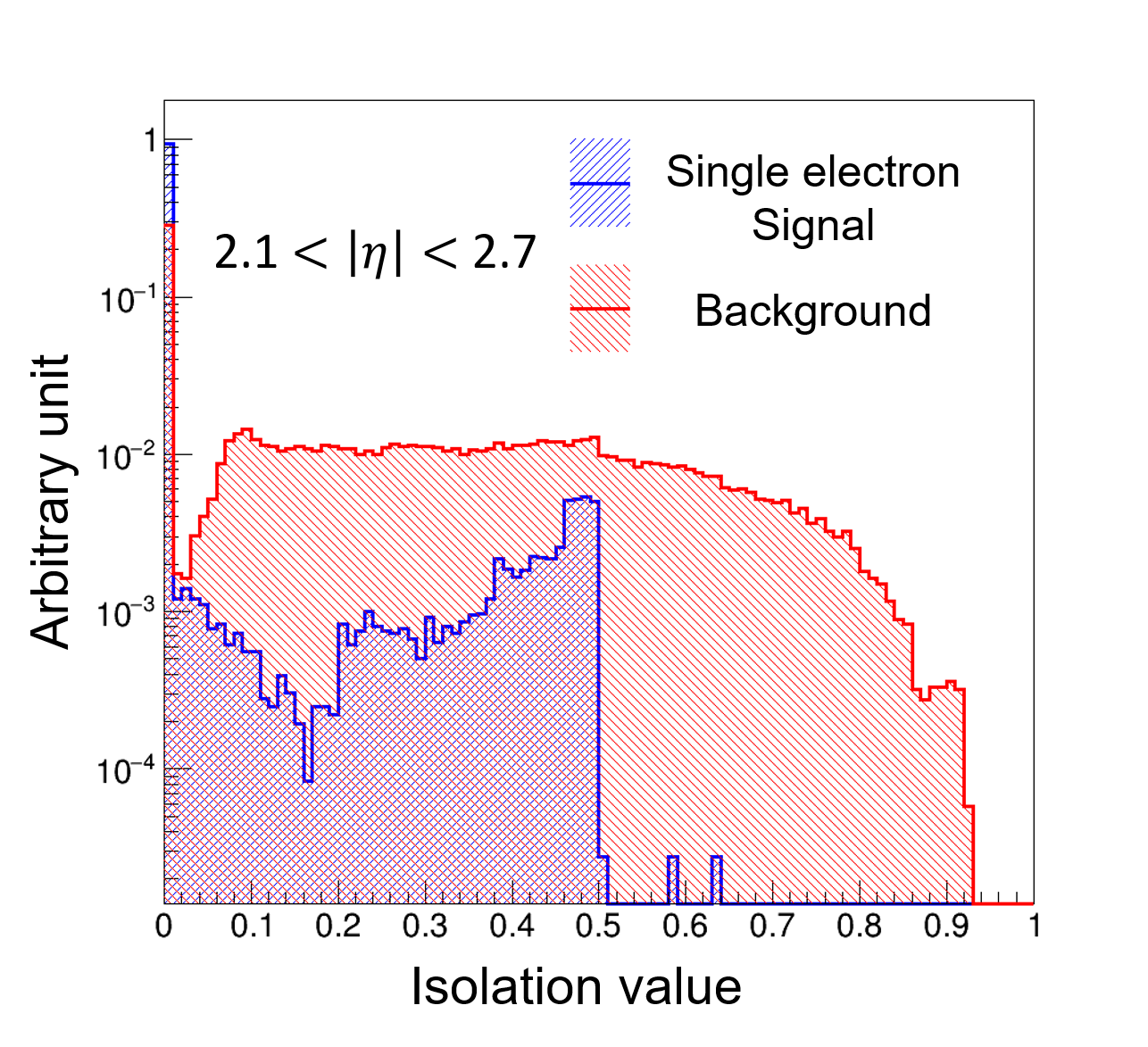
(e) Region 5

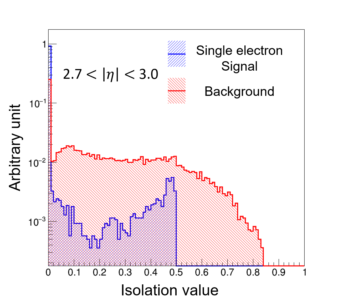
(f) Region 6

Figure 13: The pixel-based track isolation distributions of signal events (blue) and background events (red) in different $\eta$ regions.

Using these distributions, a cut value in this isolation parameter is determined for disentangling at best the signal from the background. The results are summarized in Table 4, in terms of the obtained signal efficiency and the corresponding overall background rejection, for each of the six regions in $\eta$ and the corresponding isolation cut value. Another option is also considered for the two largest $\eta$ regions, corresponding to $\eta>2.1$, for an electron of 20 GeV and results are shown in Table 5.

$\eta$ range	Isolation cut value	Signal efficiency	Background rejection
$|\eta|<$ 0.8	0.10	99.8%	74.2%
0.8 $<|\eta|<$ 1.4	0.10	99.6%	54.7%
1.4 $<|\eta|<$ 1.7	0.17	99.6%	53.0%
1.7 $<|\eta|<$ 2.1	0.28	98.0%	59.0%
2.1 $<|\eta|<$ 2.7	0.27	95.4%	46.3%
2.7 $<|\eta|<$ 3.0	0.21	94.8%	45.7%

Table 4: The signal efficiency and background rejection obtained with the pixel track isolation algorithm for each $\eta$ region, for an electron of 20 GeV.

$\eta$ range	Isolation cut value	Signal efficiency	Background rejection
2.1 $<|\eta|<$ 2.7	0.44	98.0%	22.5%
2.7 $<|\eta|<$ 3.0	0.47	98.0%	17.6%

Table 5: The signal efficiency and background rejection obtained with the pixel track isolation algorithm for the two largest $\eta$ regions, corresponding to $|\eta|>2.1$, for an electron of 20 GeV.

A signal efficiency of 99.8% with a background rejection of 75% is obtained in the central barrel region i.e. for $\eta$ up to 0.8. The signal efficiency remains at about the same value between 99.8 and 99.6% with a background rejection between 55 and 59% for $\eta$ between 0.8 and 2.1.

It then slightly drops to 95.8% and 95.2% while keeping the background rejection at around 45% in the forward region i.e. $\eta$ between 2.1 and 3.0, if we choose to slightly decrease the performance in signal efficiency while we maintain a relatively high background rejection. This is the option 1. A second option (option 2) is based on choosing to keep a very high efficiency around 98% for the two more forward regions while the rejection rate is decreased to about 20%, with thus a bit higher L1 trigger rate.

Because of a simplified detector layout and simulation, the results reported here are underestimated with respect to what will be achievable with the sophisticated designs of the ATLAS and CMS pixel detectors for HL-LHC also serving as examples for future machines.

5 Results and Performances

This section summarized the main results of the performance studies. It stresses the benefits of the L1 trigger performances by including the pixel information in the electron trigger as an example. Section 6 summarizes the two main categories of technological challenges to be overcome to make this option feasible within the HL-LHC scenario. This implies the Pixel Front-End ASIC and the real-time related algorithms to perform this triggering scheme, thanks also to the novel development in the processor technology. Section 7 concludes by showing the perspectives for a possible beyond baseline upgrade at HL-LHC and also for application to future colliders.

5.1 Performance in real-time selection: efficiency and rate reduction

The performance of the real-time selection is measured in terms of the real-time selection efficiency (also called Level-1 trigger efficiency) over the full $\eta$ range of the detector and of the corresponding trigger rate reduction.

The efficiency of the PiXTRK real-time track reconstruction algorithm without (blue) or with (green) including the pixel charged isolation (in green for option 1 and orange for option 2 in the endcaps) is measured as the trigger efficiency for electrons with a threshold of 35 GeV in $E_{\textrm{\scriptsize T}}$.

The efficiency is shown in Fig. 14, as a function of the $\eta$ at the generator level, $|\eta_{GEN}|$, of the electron candidates for the two presented options, on the overall covered $\eta$ range by the pixel detector.

Table 6 shows the average trigger efficiency for the different L1 trigger cases in four different regions, namely:$|\eta|<$ 1.0, 1. $<|\eta|<$ 1.5, 1.5 $<|\eta|<$ 2.5 and 2.5 $<|\eta|<$ 3.0 and taking into account the two considered options for the far-end or forward regions.

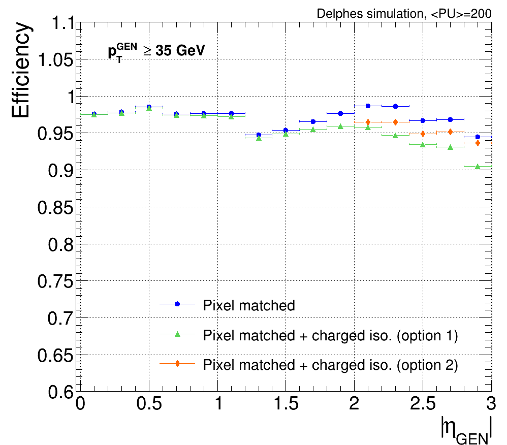
Figure 14: Real-time trigger efficiency as a function of $\eta$ at the generator level, $|\eta_{GEN}|$, for electrons of at least 35 GeV in $E_{\textrm{\scriptsize T}}$, and 200 pileup at the HL-LHC, as achieved by the PiXTRK algorithm without (blue) and with (green) pixel track isolation if option 1 or with (orange) pixel track isolation if option 2, with DELPHES based simulation.

L1 trigger	$|\eta|<$ 1.0	1.0 $<|\eta|<$ 1.5	1.5 $<|\eta|<$ 2.5	2.5 $<|\eta|<$ 3.0
Pixel matched	97.8%	95.8%	97.7%	95.2%
Pixel matched + track iso. (option 1)	97.7%	95.5%	95.2%	90.9%
Pixel matched + track iso. (option 2)			96.1%	93.9%

Table 6: Average efficiency for the electron track reconstruction of the real-time PiXTRK algorithm, in the barrel ($|\eta|<$ 1), the transition region barrel-endcap (1.0 $<|\eta|<$ 1.5), the near-endcap region (1.5 $<|\eta|<$ 2.5) and the far-endcap or forward (2.5 $<|\eta|<$ 3.0) regions.

Another important parameter in the real-time selection performances of a detector is the impact on the trigger rate reduction. This is determined as a function of L1 e/$\gamma$ object $E_{\textrm{\scriptsize T}}$ threshold, over the overall $\eta$ coverage of the detector.

The rate reduction is compared to what is achieved by the Level-1 calorimeter trigger (black), by the PiXTRK real-time reconstruction algorithm without (red), and with the pixel track isolation for the two considered options (green for option 1 and magenta for option 2). The corresponding curves, of the rate reduction as a function of the L1 e/$\gamma$ object $E_{\textrm{\scriptsize T}}$ threshold provided by the L1 EM calorimeter, for the different regions in $\eta$, namely: in the extended barrel ($|\eta|<$ 1.5), the near-endcap region (1.5 $<|\eta|<$ 2.5), the combined overall $|\eta|<$ 2.5 region and the far-endcap or forward region (2.5 $<|\eta|<$ 3.0) where tracking can only be made by the pixel detector, are shown on Fig. 15.

The results in rate reduction are summarized as well, in Table 7. It gives the average rates obtained by applying PiXTRK algorithm without or with track isolation, for the electron reconstruction in the extended barrel ($|\eta|<$ 1.5), the endcap region (1.5 $<|\eta|<$ 2.5), the overall region covered by the outer tracker ($|\eta|<$ 2.5) and the far-endcap or forward region (2.5 $<|\eta|<$ 3.0) only covered by the pixel tracker. It is worth noting that, in the considered scenario the (2.5 $<|\eta|<$ 3.0 end-cap/forward region) is only covered by the Pixel detector, from the tracking system point of view, while the endcap calorimeter covers this region.

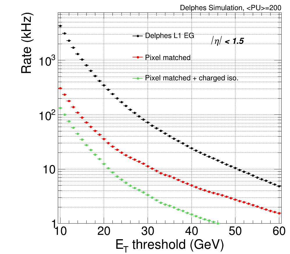
(a) Rate reduction in the barrel ($|\eta|<$ 1.5)

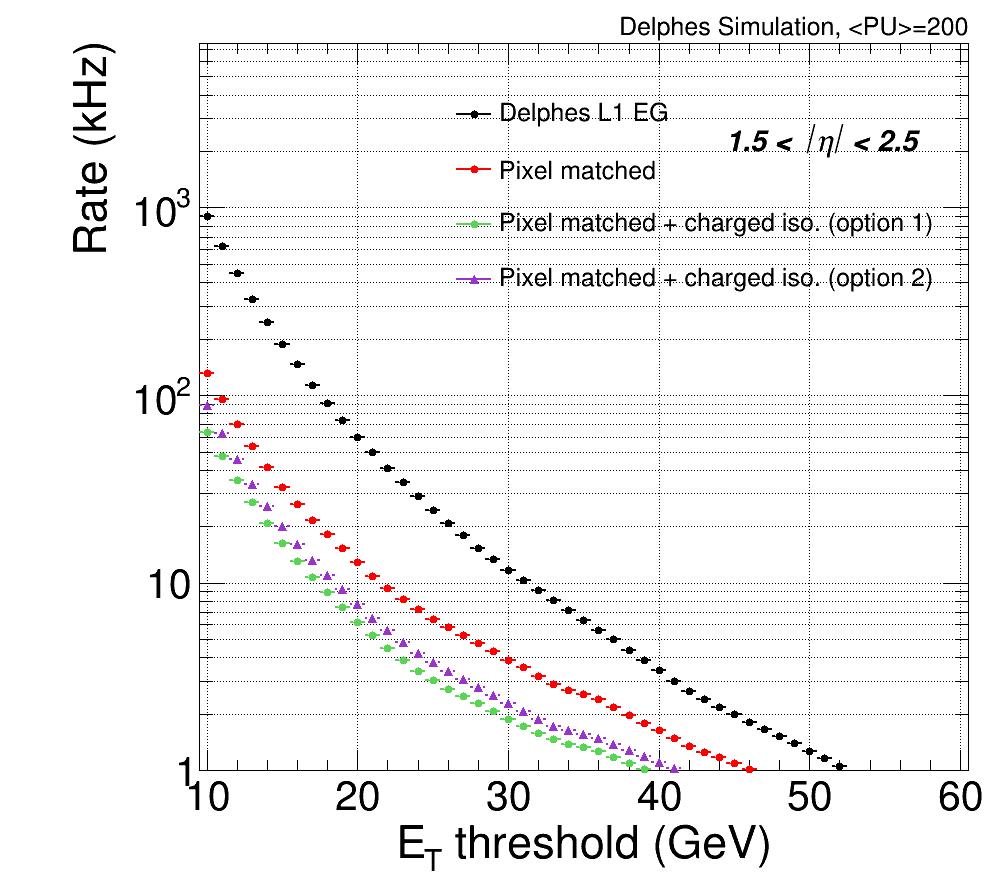
(b) Rate reduction in endcap (1.5 $<|\eta|<$ 2.5)

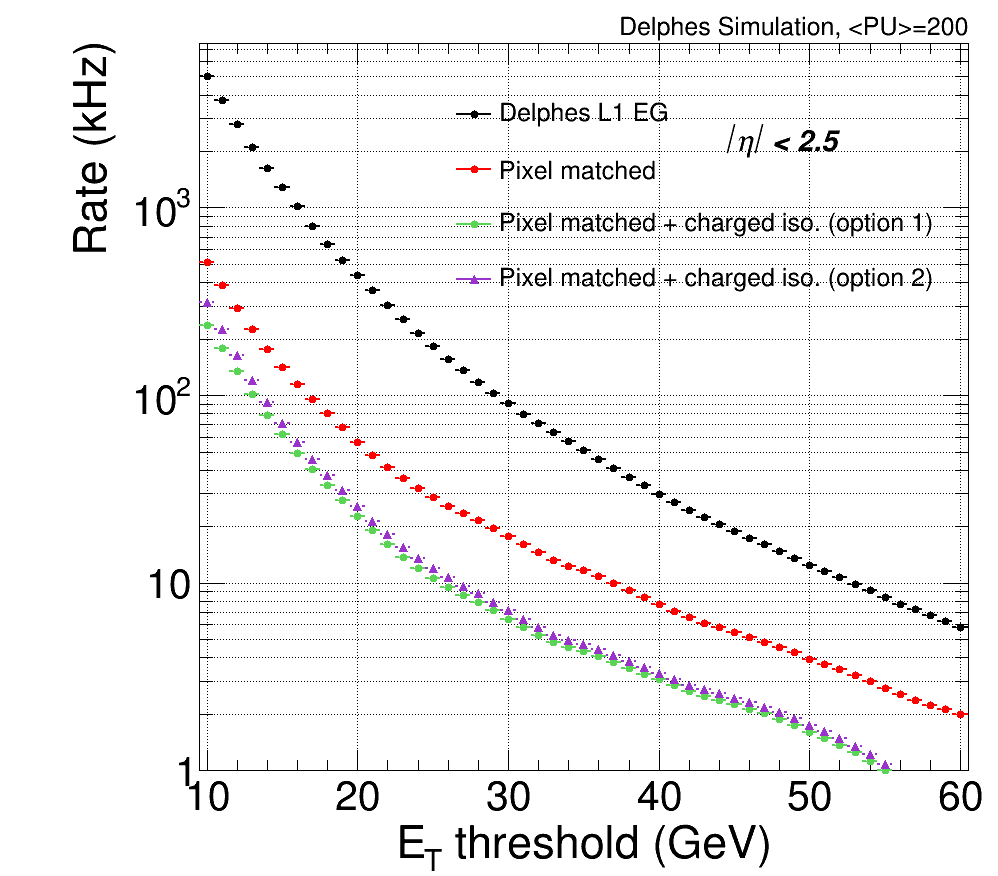
(c) Rate reduction for overall region ($|\eta|<$ 2.5)

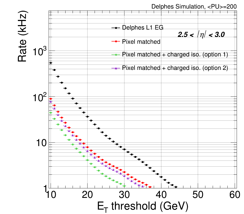
(d) Rate reduction in forward (2.5 $<|\eta|<$ 3.0)

Figure 15: Real-time trigger rate as a function of $E_{\textrm{\scriptsize T}}$ with DELPHES based simulation for different $\eta$ regions and including for the endcap and forward regions the two considered options by choosing two different isolation cut values.

L1 trigger	$|\eta|<$ 1.5		1.5 $<|\eta|<$ 2.5		2.5 $<|\eta|<$ 3.0
	Rate	Rej. factor	Rate	Rej. factor	Rate	Rej. factor
Calorimeter-only	345 kHz	-	60.0 kHz	-	36.8 kHz	-
Pixel matched	35.6 kHz	9.7	12.8 kHz	4.7	7.9 kHz	4.6
Pixel matched + track iso. (option 1)	12.4 kHz	27.8	6.2 kHz	9.7	4.1 kHz	8.9
Pixel matched + track iso. (option 2)			7.7 kHz	7.8	6.5 kHz	5.6

Table 7: Rates and rejection factor at $E_{\textrm{\scriptsize T}}=$ 20 GeV threshold obtained by PiXTRK for the electron reconstruction in the barrel ($|\eta|<$ 1.5), endcap (1.5 $<|\eta|<$ 2.5), and forward (2.5 $<|\eta|<$ 3.0) regions.

5.2 Real-time processing of the pixel detector information: further potential

Beyond the improvements in the real-time selection (or Level-1 trigger), this section summarizes the additional benefits the pixel information provides if processed in real-time. Because of its location and design, the innermost part of tracking systems, made of extremely fine granularity pixels presents the challenge of the huge data rate (thus the need for seeded handling of its information) but in counterpart offers three major virtues: closest to the beam-pipe and thus to the interaction point, low material budget, very forward expandability.

This device is thus unique for determining with a very high resolution of the primary vertex position of the events, tagging b- or c-quarks produced in the interaction (high resolution secondary vertex position), handling the pileup, discriminating tracks from bremsstrahlung, reconstructing relatively low $p_{\textrm{\scriptsize T}}$ tracks, being the tracking device linked to the endcap and forward parts of the calorimeters and the muon detectors because covering a tracking region that cannot be addressed by the outer tracker. All this is performed at the High-Level Trigger and off-line. But having these possibilities in real-time will be more and more needed by physics and achievable thanks to the advances in AI-based algorithms and new processors.

This study does not address all of them, but using the electron case, a fair amount of the potential of this device for real-time processing is shown.

By being closest to the interaction point and with the finest granularity, the vertexing capability of this device is unique. Section  3.3 describes a detailed study of how to exploit it in real-time with the electrons as a showcase. Table 8 here below, summarizes the results of this study with the performances in the resolution of the primary vertex position as determined, with the Pixel detector information for single electrons plus 200 pileup events.

$\eta$ Range	Vertex resolution
$|\eta|<$ 0.8	19.7 $\mu$m
0.8 $<|\eta|<$ 1.4	28.2 $\mu$m
1.4 $<|\eta|<$ 1.7	63.3 $\mu$m
1.7 $<|\eta|<$ 2.1	58.1 $\mu$m
2.1 $<|\eta|<$ 2.7	244 $\mu$m
2.7 $<|\eta|<$ 3.0	379 $\mu$m

Table 8: Resolution on the primary vertex position for the electron plus 200 pileup events, in the six considered regions corresponding to different $\eta$ ranges.

The z-resolution in the central region ($\eta$<1.4) is below 30 $\mu$m. It remains around 60 $\mu$m up to $\eta$ of 2.1. In the forward region, it reaches 380 $\mu$m. More generally, the vertex position resolution obtained with the pixel detector is better than an order of magnitude compared to the one obtained with the outer tracker only, as reported in the performance study, including the pixel information in a real-time b-tagging trigger  Moon_2016 .

The low material budget and again the fine granularity of this device provide other advantages of interest for the real-time processing of its information. Among these advantages, the capability to consider tracks with very low $p_{\textrm{\scriptsize T}}$ means that they can be measured them with fairly good resolution. This is addressed in detail in the study of the track isolation (Section  4). Decreasing the $p_{\textrm{\scriptsize T}}$ cut threshold for the tracks in the isolation cone from 2 GeV to 0.5 GeV diminishes the background rejection from 65% to 10% but allows keeping 99% instead of 92% of the signal events.

To optimize the real-time selection, one has to make a compromise between the efficiency and the rate reduction. It is worth noting that keeping the trigger efficiency very high to the expense of a decrease in rate reduction gives rather similar results in terms of rate reduction for $|\eta|$ up to 2.5. Instead, for $\eta>2.5$, the charged isolation does not have a real impact on rate reduction but this trigger rate is not dramatically high, and indeed still affordable.

Besides the benefits of the real-time selection, lowering the $p_{\textrm{\scriptsize T}}$ cut threshold of smaller values, has an important impact on increasing the Physics reach on a number of important topics such as Heavy Flavour Physics, rare $\tau$ lepton decays, etc.

The expandability of the pixel detector to very large values in $\eta$ is another asset of this device. It makes it unique as a tracking device in the forward regions, to be coupled with the calorimeters and the muon detectors. Although the simplified pixel layout considered here extends only to $\eta$ of 3, because of the present coverage of the endcap calorimeters for HL-LHC, this study already indicates the tracking capability and performances of the pixel detectors in the forward region as covered for the first phase (at least) of the HL-LHC. It must be noted that the present microvertex being built for HL-LHC covers up to $\eta$ of 4. It should be pointed out that, because of the Physics needs at the HL-LHC, an extension of the calorimetry and of the muon detection down to $\eta$ of 4, might be part of the second stage of the HL-LHC upgrades of the experiments for 2032. Thus, the results of this study can be extended with a still good efficiency and rejection rate for the electron case to $\eta$ of 4 and extrapolated as well to other physics objects such as muons or jets.

The extension of the current pixel detectors of both ATLAS and CMS down to $\eta$ of 4, will thus be of unique value for reconstructing forward electrons. Following the example of the electrons, muons as well as $\tau$ leptons, forward jets, or tagging of b-quarks to the forward regions (boosted objects) will be feasible, all this in real-time triggering. This will be the object of other studies on jet real-time reconstruction performances and b-tagging performances with the pixel detectors.

It is important for the physics potential at the HL-LHC, and even more when considering future machines with higher c.m. energy. to extend the tracker to larger $\eta$. In that later case, preliminary designs for FCC-hh FCC for instance, extend the usable $\eta$ range of the pixel trackers to at least $|\eta|$ of 4 or even 6, because of the Physics requirements.

Besides, the HL-LHC will be a unique playground for learning how to handle these physics cases even more important at higher energy machines.

6 Pixel information in real-time: Main Technological challenges

This section underlines the feasibility of including the microvertex detector information in the real-time selection stage, i.e. at 40 MHz input rate and latency of order ten microseconds (namely 10 or 12.5 $\mu$s for ATLAS or CMS respectively). This mainly adverts to very demanding challenges on 1) the hardware aspect, especially on the Front-End Electronics (FEE), and 2) the software computing aspect with the implementation of fast (real-time) and highly performing algorithms and processor units. The first challenge is primarily on the Front-End pixel ASIC, sitting at the forefront of the signal processing. The second challenge is on an intelligent processing of the Front-End information delivered by the FEE, able to provide within the short trigger latency, relevant and beneficial information, further improving this first selection stage. This second challenge is related to real-time algorithms and fast new processors. These two challenges are briefly tackled below.

6.1 The Front-End hardware challenges

The Front-End ASIC, PSI46V2  Barbaro-PSI_2006 , of the first Pixel detector designed and built by the PSI group in CMS already addressed the implementation of the pixel information in the L1 trigger via the double column concept. A cluster multiplicity counter, i.e. a fast trigger signal was made available to the L1 trigger system. It included two thresholds that could be set by this mechanism: one setting the minimum number of hits within a double column, whereas the other tuning the number of hit double columns above which a trigger signal is issued.

Both ATLAS and CMS are developing a FE ASIC within the international R&D collaboration RD53 Garcia-Sciveres:2113263 . ATLAS pioneered some of the key features of this device, with the development of a new FE ASIC for the upgrade of the ATLAS Microvertex at the LHC Phase-1 GARCIASCIVERES2011S155 ; Garcia_Sciveres_2018 . This FE chip (FEI4) includes together with advanced processing of the pixel hits, two main features, namely: i) the logic to gather several pixel hits within a single “cluster” (clusterization) and ii) a two-trigger-signal scheme by adding to the usual 40 MHz L1 trigger, a second fast real-time trigger signal (labeled as L0). The L0 trigger allows a prompt extraction of the clusters of pixel hits that correspond to the 40 MHz trigger and their transmission to the next level of signal processing. These two features are essential assets to perform real-time signal processing at the front-end level.

The experience gained with this first generation of new “intelligent” FE ASICs operating in harsh HL-LHC conditions will be instrumental in the development of the updated version which will be able to fully address the challenges of a real-time L1 pixel-based trigger.

6.2 The use of AI and new Processor tools

Over the last 5 years, the use of AI-based tools in several aspects of the signal and data processing chain is making impressive advances in the HEP domain and especially the LHC experiments. This goes together with the increase in performances of the new processors (e.g. new FPGAs).

The application of AI (e.g. Neural Networks etc.) software tools allows performing sophisticated algorithms in record times and with high data rates. This is more and more developed in different triggering levels (even at the L1 level) or DAQ stages, coupled with high performance FPGA or GPU units in the LHC experiments.

Besides the use of AI at the software level, new interesting developments have recently occurred based on embedding AI in the hardware processing of the detector signal. The developed hls4ml tool hls4ml is an open-source software-hardware codesign workflow to interpret and translate machine learning algorithms for implementation with both FPGA and ASIC technologies. It allows near-sensor real-time processing. It is already used in the design and fabrication of a reconfigurable neural network ASIC for detector front-end data compression at HL-LHC MLhardware-appli . Preliminary applications to high granularity devices (pixel detectors or high granularity calorimeters) are considered or under study.

The study reported in this paper is done with simple algorithms and software tools (e.g. LUTs) easily performed with the present software and processor tools (current FPGAs). It stresses the improvements in the trigger performances by including the pixel information. A benchmarking platform using the new hardware based developments (i.e. new Front-End ASIC design and AI-based tools) applied to a pixel detector demonstrator is the subject of an R&D, to be reported in another paper.

7 Perspectives and concluding remarks

A second phase of the HL-LHC is foreseen with the aim to reach an even higher instantaneous luminosity (7.5$\times$10³⁴cm^-2s^-1) and thus get 4 ab^-1 total integrated luminosity by the end of HL-LHC atlasTDR-TDAQ . Besides, a possible slight increase of the LHC collider c.m. energy could be feasible in the labeled Run 4 (after 2030). This is part of the worldwide developments on Higher Field Magnets for future hadron colliders. Furthermore, various detector upgrade stages are part of the routine life of the experiments at long-life machines. This will apply to the HL-LHC which will last for more than 10 years.

ATLAS first defined an evolution scenario for handling the Run 4 challenges atlasTDR-TDAQ . It keeps the 3 stages strategy as reminded in this paper but with an increased input rate at L1 (up to 2 or 4 MHz) and an extension of the L1 trigger latency to 30 or 35 $\mu$s. Within this scheme as in the first part of the HL-LHC, the pixel information will be partly included in the overall track trigger of the ATLAS experiment part of the L1 trigger, working with 2 up to 4 MHz reduced input rate, after the L0-trigger which works with the full 40 MHz input rate. This is now superseded by the amendment to the TDR atlasTDR-TDAQ-Add . The objective is to keep, over the whole HL-LHC, the same trigger scheme and to overcome the machine’s increased performances in a possible second stage of HL-LHC, thanks to a revised Event Filter, as described in this amendment. This Event Filter relies on the advances in the industrial world, on CPUs, GPUs, and FPGAs as well as on the AI field. The ongoing impressive progress in these areas will allow for the building of a fancy and highly performing heterogeneous system associated with sophisticated and quite efficient algorithms on the software side. CMS has developed a Track Trigger detector and associated FEE for the outer Tracker part (all but the Microvertex) able to work at a 40 MHz input rate. The Pixel information is used at the High-Level Trigger stage.

Moreover, let us stress the interest in developing a similar first level trigger for the pixel based timing detectors, under active R&D for HL-LHC. The accurate timing information at the first level trigger will be of utmost importance (e.g. increase of pile-ups). This is a piece of major information to incorporate at the first level trigger in the forthcoming trigger system upgrades.

The performance-based study presented in this paper goes beyond the ATLAS and CMS HL-LHC track trigger present scenarios by showing the benefits of using the Microvertex information, in the trigger architecture, at the real-time level. It shows how including the information from this essential detector, will improve the overall trigger real-time selection performances. This will be highly beneficial for increasing the Physics potential of these detectors. It will allow extracting most of the HL-LHC era Physics and get ready for the next generation(s) of detectors to be running at future high-energy machines. The setting up of a dedicated benchmark platform including the hardware devices and software tools will be the subject of another paper.

Appendix A The DELPHES simulation

The DELPHES simulation, used as a framework for these performance studies, is detailed in this Appendix. As pointed out in Section 1, including the pixel detector within the overall L1 trigger CMS upgrade for HL-LHC has not been endorsed by the CMS collaboration CMS-phase2L1TDR . Therefore, the work reported here is performed at a “generic level” and in a more general approach, but also keeping the overall CMS-Phase2 upgrade as an example case.

Three types of simulated MC samples are generated using DELPHES in this study: (i) 5 million single electron gun events without pileup to measure 3$\sigma$ boundaries of signal windows; (ii) 1 million single electron gun events with 200 PU for measuring the L1 trigger efficiency; (iii) 10 million of minimum bias events with 200 PU for estimating the L1 trigger rate; (ii) and (iii) samples are used for the pixel-based charged isolation algorithm.

The calorimeter only information (no tracking included) allows the defining of the so-called L1 electron/photon (L1 e/$\gamma$) objects. A more precise L1 e/$\gamma$ definition is provided through the L1 tower objects. The Phase-2 CMS calorimetry is taken as a showcase. The barrel calorimeter made of crystals has a granularity of (0.0174, 0.0174) in ($\eta,\phi$)  CMS-barrelECAL . The endcap calorimeter, based on silicon sensors, provides position resolution better than 1 mm because of the small cell sizes; the angular uncertainty in $\theta$ is of 7 mrad for a $p_{\textrm{\scriptsize T}}$ shower of 25 GeV without corrections and tuning CMS-HGCAL .

As for the Phase-2 upgrades of ATLAS and CMS  ATLAS-phase2tracker ; CMS-phase2tracker , the microvertex detector simulation considers small pitch silicon pixel sensors of 100-150 $\mu$m thickness, with pixel size of 50$\times$50 $\mu$m² for the barrel part, and 25$\times$100 $\mu$m² for the endcap and forward parts. Pixel clusters are built from contiguous pixels. A threshold of 1200 electrons is set in the Time over Threshold based readout, with 4 bit charge resolution CMS-phase2tracker .

DELPHES provides a simplified description of the two L1 key parameters, i.e. the trigger towers for the calorimetry, and the L1 tracks for the tracking system. These are the physical/detector entities we refer to at Level-1; they are described in detail in a full detector simulation such as CMSSW for CMS. Tower objects are produced to match the granularity of the Phase-2 CMS calorimeter. Pixel clusters are simulated from the tracks in DELPHES simulation by smearing position resolution to be consistent for instance with that of CMSSW.

The resolutions of the $\phi$ and $\eta$ position parameters of the produced DELPHES L1 e/$\gamma$ objects are shown in Fig. 16 and Fig. 17. The angular resolutions $\Delta\phi=\phi_{\textrm{\scriptsize gen}}-\phi_{\textrm{\scriptsize tower}}$ and $\Delta\eta=\eta_{\textrm{\scriptsize gen}}-\eta_{\textrm{\scriptsize tower}}$ are defined as a function of the generator level (gen-level) electron $p_{\textrm{\scriptsize T}}$, while the vertex correction is applied to the L1 e/$\gamma$ objects. The parameters $\phi_{\textrm{\scriptsize gen}}$ and $\eta_{\textrm{\scriptsize gen}}$ are the “true” generated $\phi$ and $\eta$ position parameters. The parameters $\phi_{\textrm{\scriptsize tower}}$ and $\eta_{\textrm{\scriptsize tower}}$ are the position parameters in $\phi$ and $\eta$ of the single crystal tower in the barrel EM calorimeter, respectively the elementary tower element in the HGCAL endcap EM calorimeter. For measuring the position resolution of L1 e/$\gamma$ objects, a single electron sample is used. It is worth noting that because of the highest granularity of the HGCAL end cap calorimeter, the region with $\eta$ above 1.7 shows a higher resolution.

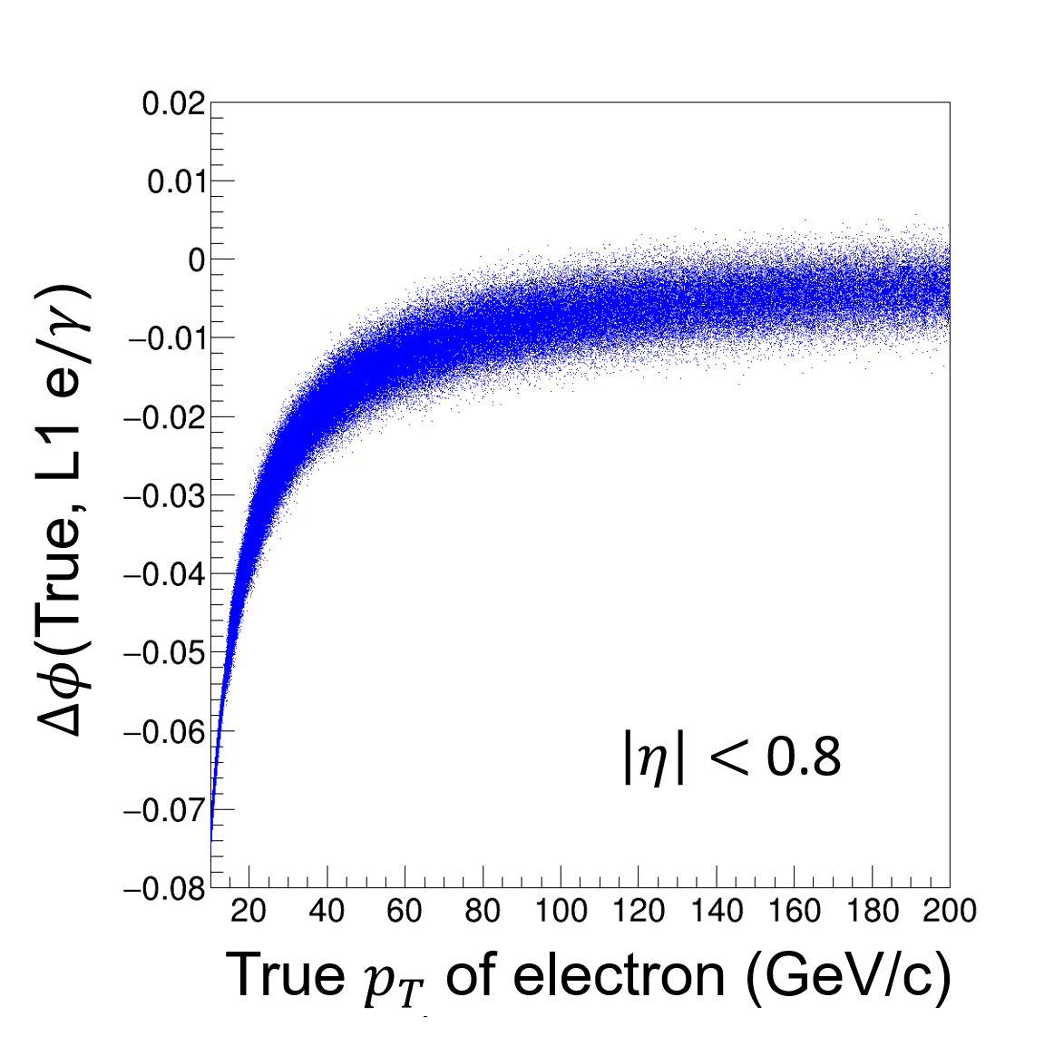
(a)

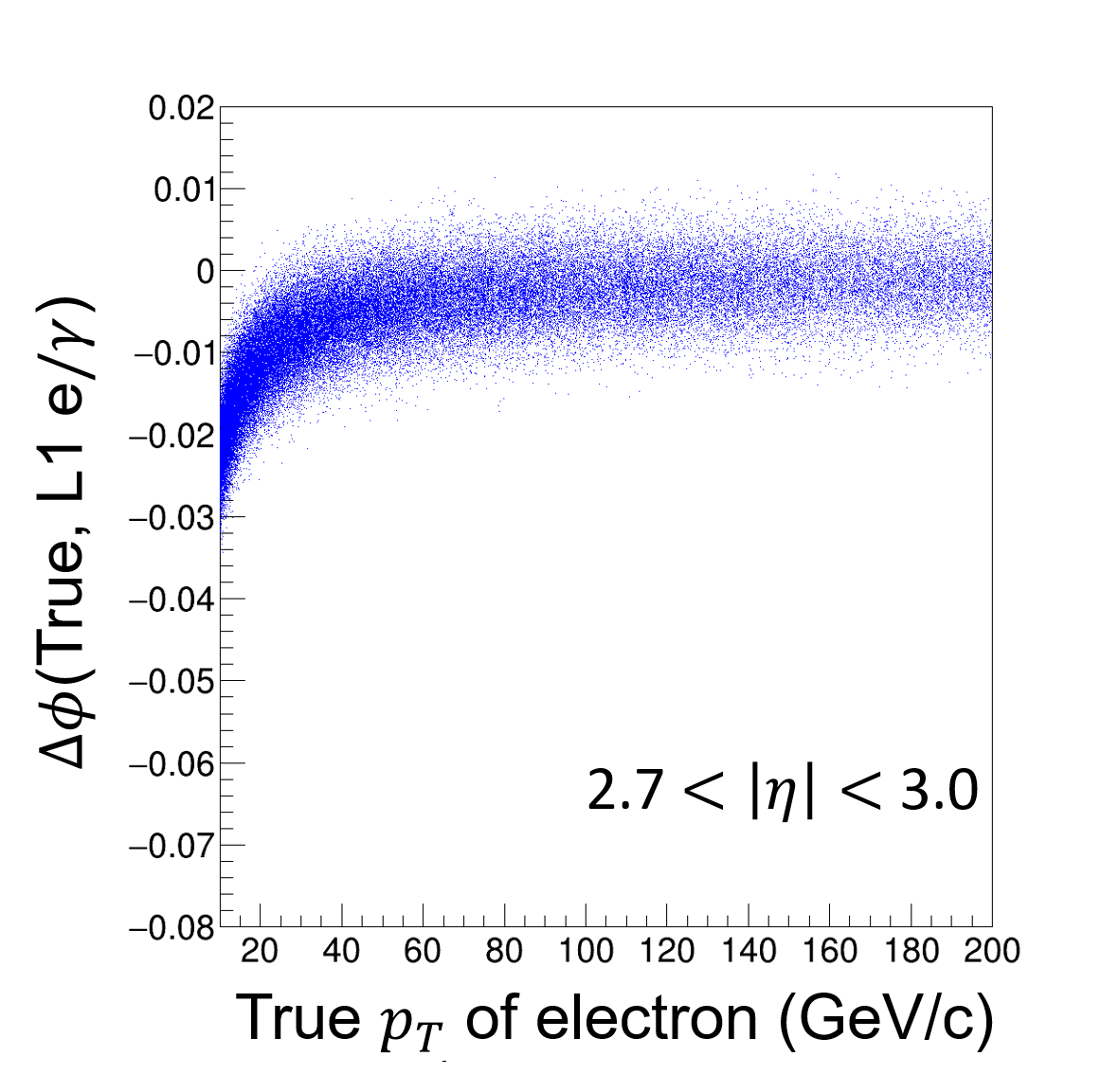
(b)

Figure 16: $\Delta\phi$ distributions showing the difference in $\phi$ between the “true” $\phi$ i.e. from the gen-level electron and the $\phi$ from the L1 e/$\gamma$ object, as a function of the “true” gen-level $p_{\textrm{\scriptsize T}}$, for the considered $\eta$ regions. The corresponding $\Delta\phi$ distributions for the positrons are symmetrical w.r.t. $\Delta\phi$ = 0 axis, to the ones of the electrons.

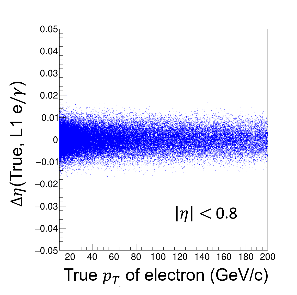
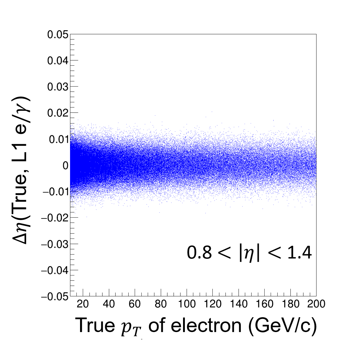
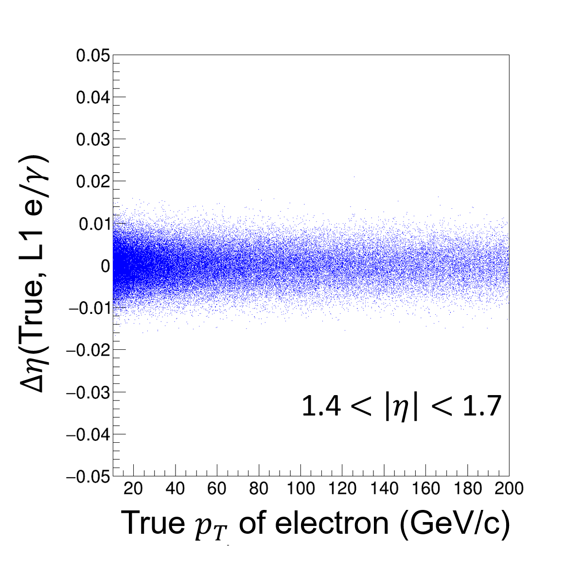
(a)

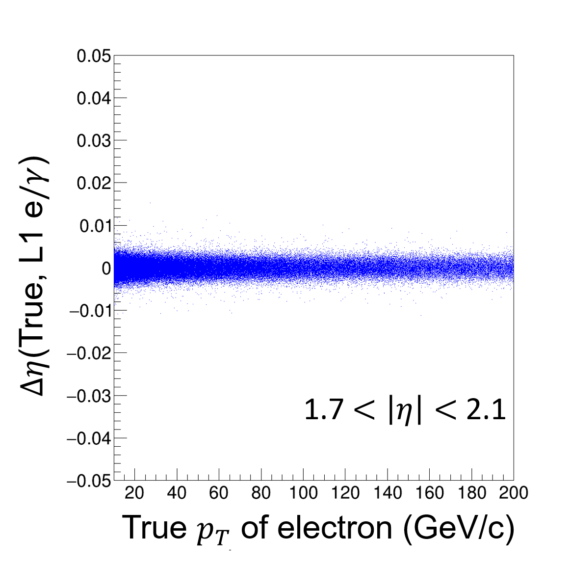
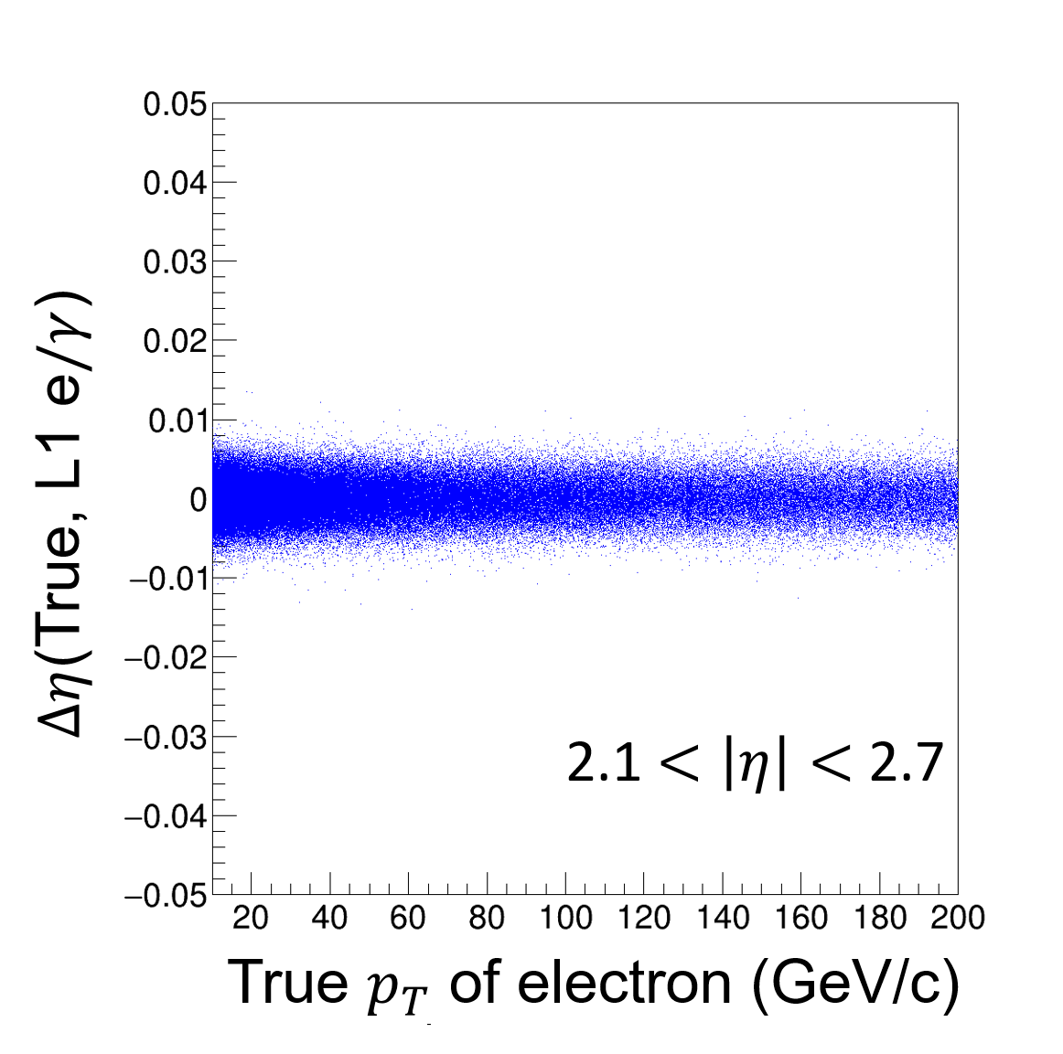
(b)

Figure 17: $\Delta\eta$ distributions representing the difference in $\eta$ between the “true” $\eta$ i.e. from the gen-level electron and the one from the L1 e/$\gamma$ object, as a function of the “true” gen-level $p_{\textrm{\scriptsize T}}$, for the considered $\eta$ regions. Positrons have the same $\Delta\eta$ distributions.

Appendix B $\Delta\phi$-LUT for real-time pixel-based track reconstruction algorithm

B.1 Step 2 cases

L1 e/$\gamma$ $E_{\textrm{\scriptsize T}}$ (GeV)	10	11	12	13	14	15	16	17	18	19	20	22	24	26	28	30	35	40	45	50
3$\sigma$ upper boundary	0.089	0.082	0.077	0.072	0.069	0.065	0.063	0.060	0.058	0.056	0.054	0.050	0.047	0.045	0.043	0.041	0.038	0.035	0.033	0.031
3$\sigma$ lower boundary	0.048	0.043	0.038	0.034	0.030	0.027	0.025	0.022	0.020	0.018	0.016	0.013	0.011	0.009	0.007	0.005	0.002	-0.001	-0.003	-0.004

Table 9: Step 2: $\Delta\phi$-LUT for $\eta$ Region 1, 2, 3, i.e. $\eta$<1.7

L1 e/$\gamma$ $E_{\textrm{\scriptsize T}}$ (GeV)	10	11	12	13	14	15	16	17	18	19	20	22	24	26	28	30	35	40	45	50
3$\sigma$ upper boundary	0.071	0.067	0.063	0.060	0.057	0.054	0.052	0.050	0.048	0.046	0.045	0.042	0.040	0.039	0.037	0.036	0.033	0.031	0.029	0.028
3$\sigma$ lower boundary	0.033	0.029	0.025	0.022	0.020	0.017	0.015	0.014	0.012	0.010	0.009	0.007	0.005	0.003	0.002	0.000	-0.002	-0.004	-0.006	-0.007

Table 10: Step 2: $\Delta\phi$-LUT for $\eta$ Region 4, i.e. 1.7<$\eta$<2.1.

L1 e/$\gamma$ $E_{\textrm{\scriptsize T}}$ (GeV)	10	11	12	13	14	15	16	17	18	19	20	22	24	26	28	30	35	40	45	50
3$\sigma$ upper boundary	0.048	0.046	0.043	0.042	0.040	0.039	0.037	0.036	0.035	0.034	0.033	0.032	0.031	0.030	0.029	0.028	0.027	0.026	0.025	0.024
3$\sigma$ lower boundary	0.010	0.008	0.006	0.005	0.004	0.003	0.002	0.001	0.000	-0.001	-0.001	-0.003	-0.004	-0.005	-0.006	-0.006	-0.008	-0.009	-0.010	-0.011

Table 11: Step 2: $\Delta\phi$-LUT for $\eta$ Region 5, i.e. 2.1<$\eta$<2.7.

L1 e/$\gamma$ $E_{\textrm{\scriptsize T}}$ (GeV)	10	11	12	13	14	15	16	17	18	19	20	22	24	26	28	30	35	40	45	50
3$\sigma$ upper boundary	0.037	0.035	0.034	0.032	0.031	0.031	0.030	0.029	0.028	0.028	0.027	0.026	0.026	0.025	0.025	0.024	0.023	0.022	0.022	0.021
3$\sigma$ lower boundary	0.000	-0.001	-0.002	-0.003	-0.004	-0.004	-0.005	-0.006	-0.006	-0.007	-0.007	-0.008	-0.009	-0.010	-0.010	-0.011	-0.011	-0.012	-0.013	-0.013

Table 12: Step 2: $\Delta\phi$-LUT for $\eta$ Region 6, i.e. 2.7<$\eta$<3.0.

B.2 Step 3 cases

L1 e/$\gamma$ $E_{\textrm{\scriptsize T}}$ (GeV)	10	11	13	15	19	24	35	50
3$\sigma$ upper boundary	0.006	0.005	0.005	0.004	0.004	0.003	0.003	0.002
3$\sigma$ lower boundary	0.002	0.002	0.001	0.001	0.000	0.000	-0.001	-0.001

Table 13: Step 3: $\Delta\phi$-LUT for $\eta$<0.8, with pixel track reconstruction using the beam origin B0, and the two innermost barrel layers 1 and 2, thus the triplet (B0L1L2).

L1 e/$\gamma$ $E_{\textrm{\scriptsize T}}$ (GeV)	10	13	19	35
3$\sigma$ upper boundary	0.007	0.006	0.005	0.004
3$\sigma$ lower boundary	0.001	0.000	-0.001	-0.002

Table 14: Step 3: $\Delta\phi$-LUT for 1.7<$\eta$<2.1, with the pixel track reconstruction using the beam origin B0, the innermost barrel layer and nearest to barrel disk, thus triplet (B0L1D1).

L1 e/$\gamma$ $E_{\textrm{\scriptsize T}}$ (GeV)	10	12	19
3$\sigma$ upper boundary	0.006	0.005	0.004
3$\sigma$ lower boundary	0.000	-0.001	-0.002

Table 15: Step 3: $\Delta\phi$-LUT for 2.1<$\eta$<2.7, with the pixel track reconstruction using the beam origin B0, the second and third nearest to barrel disks, thus triplet (B0D2D3).

Appendix C Method for the determination of the $p_{\textrm{\scriptsize T}}$ of the track based on the pixel clusters

We reconstruct in the transverse plane the circle passing by the B0 coordinate in that plane and two of the pixel clusters of the considered track. The reconstructed circle is rotated by an azimuthal angle $\phi$ with respect to the electron candidate (Fig. 18).

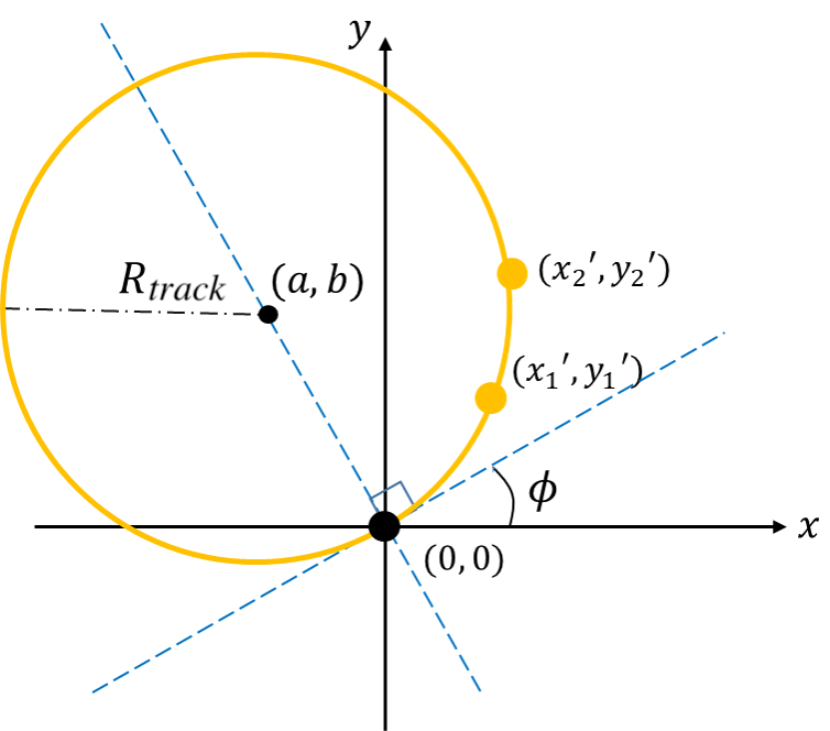
(a) Before rotation

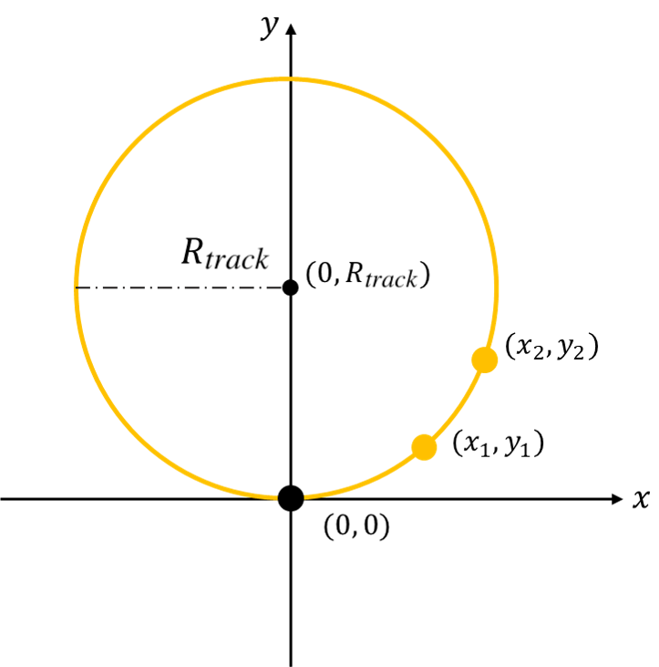
(b) After rotation

Figure 18: Schematic of the reconstructed circle in the transverse plane before rotation (a) and after rotation (b).

The rotated coordinates can be expressed with the following equations:

$$\begin{split}x_{i}=x_{i}^{{}^{\prime}}\,cos(-\phi)-y_{i}^{{}^{\prime}}\,sin(-\phi)\\ y_{i}=x_{i}^{{}^{\prime}}\,sin(-\phi)+y_{i}^{{}^{\prime}}\,cos(-\phi)\end{split}$$ (14)

where $i=$ 1 or 2. The equation of the circle in the new rotated frame is:

$$x^{2}+(y-R_{track})^{2}=R_{track}^{2}$$ (15)

By substituting two rotated coordinates $x_{i}$ and $y_{i}$ into Equation 15, we obtain:

$$\begin{split}x_{1}^{2}+(y_{1}-R_{track})^{2}=R_{track}^{2}\\ x_{2}^{2}+(y_{2}-R_{track})^{2}=R_{track}^{2}\end{split}$$ (16)

Replacing $x_{i}^{2}+y_{i}^{2}$ by $R_{i}^{2}$ after expanding Equation 16, we get:

$$\begin{split}R_{1}^{2}-2y_{1}R_{track}=0\\ R_{2}^{2}-2y_{2}R_{track}=0\end{split}$$ (17)

And thus the radius of the circle $R_{track}$ is:

$$R_{track}=\frac{R_{1}^{2}-R_{2}^{2}}{2(y_{1}-y_{2})}\;\textrm{or}\;\frac{R_{1}^{2}+R_{2}^{2}}{2(y_{1}+y_{2})}$$ (18)

References

- (1) CMS Collaboration, The CMS tracker system project: Technical Design Report, CERN-LHCC-98-006; CMS-TDR-5.
- (2) CMS Collaboration, Addendum to the CMS Tracker TDR, CERN-LHCC-2000-16; CMS-TDR-5-add-1.
- (3) ATLAS Collaboration. Technical Design Report for the Phase-II Upgrade of the ATLAS TDAQ System, CERN-LHCC-2017-020; ATLAS-TDR-029.
- (4) V. Filiminov, B. Bauss, V. Buscher, U. Schaefer, D. Bao Ta, Global Trigger Technological Demonstrator for ATLAS Phase II upgrade, IEEE Transactions on Nuclear Science, Oct 2020, 2010.07667.
- (5) ATLAS Collaboration. Technical Design Report for the Phase-II Upgrade of the ATLAS Trigger and Data Acquisition System - Event Filter Tracking Amendment, CERN-LHCC-2022-004; ATLAS-TDR-029-ADD-1.
- (6) CMS Collaboration, The Phase-2 Upgrade of the CMS Level-1 Trigger, CERN-LHCC-2020-004; CMS-TDR-021.
- (7) CMS Collaboration, The Phase-2 Upgrade of the CMS Data Acquisition and High-Level Trigger, CERN-LHCC-2021-007; CMS-TDR-022.
- (8) A. Bocci, V. Innocente, M. Kortelainen,F. Pantaleo, M. Rovere, Heterogeneous Reconstruction of Tracks and Primary Vertices With the CMS Pixel Tracker, Frontiers in Big Data, Dec. 21, 2020, 10.3389/fdata.2020.601728.
- (9) C.-S. Moon and A. Savoy-Navarro, Level-1 pixel based tracking trigger algorithm for LHC upgrade, 2015 JINST 10 C10001.
- (10) C.-S. Moon, A level-1 pixel based track trigger for the CMS upgrade, in Proceedings of 38th International Conference on High Energy Physics, Chicago, U.S.A. (2016).
- (11) The DELPHES 3 collaboration, DELPHES 3: a modular framework for fast simulation of a generic collider experiment, JHEP 02 (2014) 057.
- (12) Torbjörn Sjöstrand et al., An introduction to PYTHIA 8.2, Comput. Phys. Commun. 191 (2015) 159.
- (13) ATLAS Collaboration, Technical Design Report for the ATLAS Inner Tracker Pixel Detector, CERN-LHCC-2017-021; ATLAS-TDR-030.
- (14) CMS Collaboration, The Phase-2 Upgrade of the CMS Tracker, CERN-LHCC-2017-009; CMS-TDR-014.
- (15) V. Rekovic, L1 Trigger Emulator Phase-2 Upgrade Instructions, https://twiki.cern.ch/twiki/bin/view/CMSPublic/SWGuideL1TPhase2Instructions#CMSSW_10_1_7.
- (16) CMS Collaboration, The Phase-2 Upgrade of the CMS Barrel Calorimeters, CERN-LHCC-2017-011; CMS-TDR-015.
- (17) CMS Collaboration, The Phase-2 Upgrade of the CMS Endcap Calorimeter, CERN-LHCC-2017-023; CMS-TDR-019.
- (18) Clement Helsens, Michelangelo L. Mangano, Micehel Selvaggi, Requirements from physics for the FCC-hh detector design, CERN-FCC-PHYS-2020-0004.
- (19) H.Chr.Kaestli, M. Barbaro, W.Erdmann, Ch. Hoermann, R. Horisberger, D.Kotlinski, B.Meier, Design and Performance of the CMS Pixel Detector Readout Chip, Nucl. Instrum. Meth. , A 565 (2006), 188 - 194.
- (20) RD53 Collaboration, RD53A Integrated Circuit Specifications, CERN-RD53-PUB-15-001.
- (21) Maurice Garcia-Sciveres et al., The FE-I4 pixel readout integrated circuit, Nucl. Instrum. Meth. A 636 (2011) S155.
- (22) Maurice Garcia-Sciveres and Norbert Wermes, A review of advances in pixel detectors for experiments with high rate and radiation, Rep. Prog. Phys. 81 (2018) 066101.
- (23) Farah Fahim et al, hls4ml: An Open-Source Codesign Workflow to Empower Scientific Low-Power Machine Learning Devices, arXiv:2103.05579.
- (24) Giuseppe Di Guglielmo et al, A reconfigurable neural network ASIC for detector, front-end data compression at the HL-LHC, arXiv:2105.01683v1.