Enhanced Fast Iterative Shrinkage Thresholding Algorithm For Linear Inverse Problem

Abstract

The linear inverse problem emerges from various real-world applications such as Image deblurring, inpainting, etc., which are still thrust research areas for image quality improvement. In this paper, we have introduced a new algorithm called the Enhanced fast iterative shrinkage thresholding algorithm (EFISTA) for linear inverse problems. This algorithm uses a weighted least square term and a scaled version of the regularization parameter to accelerate the objective function minimization. The image deblurring simulation results show that EFISTA has a superior execution speed, with an improved performance than its predecessors in terms of peak-signal-to-noise ratio (PSNR), particularly at a high noise level. With these motivating results, we can say that the proposed EFISTA can also be helpful for other linear inverse problems to improve the reconstruction speed and handle noise effectively.

I Introduction

We have taken Image deblurring as a linear inverse problem to demonstrate our proposed iterative reconstruction algorithm. A linear inverse problem in the form of a discrete system can mathematically be represented as,

$$b=Ax_{org}+w,$$ (1)

where $b\in\mathbb{R}^{M}$, $A\in\mathbb{R}^{M\times N}$ are known, $w$ is the unknown noise, and $x_{org}\in\mathbb{R}^{N}$ is the ”true” and unknown image to be estimated. Image deblurring is the process in which we estimate the underlying image from its blurred image. In the case of image deblurring problems, $b$ represents the blurred image, and $A$ represents the blur operator.

A classical approach to this estimation problem is the Least Squares (LS) approach. In which we minimize the square error of the deblurred image for the problem (1). It is represented as

$$\hat{x}_{LS}=\arg\min_{x}\frac{1}{2}\|Ax-b\|_{2}^{2}.$$ (2)

In many applications like image deblurring, it is often found that $A$ is ill-conditioned. Normally we have $M<N$, which indicates that the inverse problem is ill-poised and has infinitely many solutions. In such cases, the LS solution gives a huge norm and it becomes meaningless. To overcome this problem, we use different regularization methods to stabilize the solution. Among them, the $l_{1}$ regularization method has received considerable attention in the image processing literature.

In regularization methods, the problem (1) can be recast as

$$\hat{x}=\arg\min_{x}f(x)+g(x),$$ (3)

where $f(x)=\frac{1}{2}\|Ax-b\|_{2}^{2}$, and $g(x)$ is the regularization function. $l_{1}$ regularization term refers to $\|x\|_{1}$, the sum of the absolute value of the components. Generally, it is used to induce sparsity in the optimal solution. In this case, $g(x)=\lambda\|x\|_{1}$, where $\lambda$ is the regularization parameter that trade-off $f(x)$ and $\|x\|_{1}$. To solve the problem (3), there are a number of first-order gradient-based approaches like Iterative Shrinkage Thresholding Algorithm (ISTA) [1], Fast ISTA (FISTA) [2], Monotone FISTA (MFISTA) [3], and Improved FISTA (IFISTA) [4].

Starting with an initial guess $x_{0}$, a gradient descent (GD) based iterative solution of (2) can be obtained by using the following step.

$$x_{k+1}= x_{k}-\eta\nabla f(x_{k}),$$ (4)

where $x_{k}$ is $k^{\text{th}}$ estimation of $x$, the step size is $\eta$, the gradient of $f(x)$ for $x_{k}$ is $\nabla f(x_{k})=A^{T}(Ax_{k}-b)$. The step size $\eta$ can be chosen in between $0$ and ${2}/{\lambda_{\text{max}}(A^{T}A)}$, with ${\lambda_{\text{max}}(A^{T}A)}$ being maximum eigenvalue of the matrix $A^{T}A$. In order to find an iterative solution to (3), ISTA uses a proximal operator followed by the iteration mentioned in (4). It iterates $x_{k+1}$ as

$$x_{k+1}=S_{\lambda\eta}[x_{k}-\eta\nabla f(x_{k})]$$

where $S_{\gamma}:\mathbb{R}^{n}\rightarrow\mathbb{R}^{n}$ is the proximal operator, defined as

$$S_{\gamma}[x]^{[i]}=\max\left(0,|x^{[i]}|-\gamma\right).\text{sign}\left(x^{[i]}\right),$$

where $x^{[i]}$ refers to the $i^{\text{th}}$ entry of a vector $x$, $\gamma$ is a positive real number, and $\text{sign}\left(.\right)$ refers to the signum function that gives the sign of any input real number. This operator is also famously known as the shrinkage operator.

Since ISTA iterations converge slowly at the rate of $O(\frac{1}{k})$, where $k$ is the iteration number. In order to improve the speed, a variant of ISTA called FISTA has been proposed by Beck et al. FISTA integrates the Nesterove’s momentum into ISTA to achieve a faster convergence rate of $O(\frac{1}{k^{2}})$ [2]. The following are the iteration steps of FISTA.

$$x_{k+1}= S_{\lambda\eta}[y_{k}-\eta\nabla f(y_{k})]$$

where $y_{k}$ is the Nesterove’s momentum that combines previous two estimates $x_{k}$ and $x_{k-1}$. That is

$$y_{k}= x_{k}+\frac{\alpha_{k-1}-1}{\alpha_{k}}(x_{k}-x_{k-1}),$$ (5)

where $\alpha_{k}$’s are generated sequence of numbers.

To further accelerate the convergence of FISTA, Zulfiquar et al. has proposed IFISTA [4]. The contribution of IFISTA is to fast-forward the least square gradient descent iteration (4) by $n$ steps as follows.

$$x_{k+1}=x_{k}-\eta W_{n}\nabla f(x_{k})$$ (6)

where $W_{n}$ is the weighting matrix and which is defined as

$$W_{n}= \sum_{i=1}^{n}\prescript{n\mkern-0.5mu}{}{C}_{i}(-1)^{i-1}(\eta A^{T}A)^{i-1}.$$ (7)

Since $W_{n}$ is pre-determined, the computation cost per iteration will remain the same as that of FISTA. The image de-blurring results in [4] show that the IFISTA algorithm provides competent image restoration capability with an improved convergence rate than the FISTA Algorithm.

We should note that the demonstration is only done for low Additive White Gaussian Noise (AWGN) scenarios. However, increasing the power of AWGN, the objective value starts diverging over the iteration of IFISTA, which can be seen from Fig. 1 of our result section. In this paper, we have proposed an Enhancement of FISTA for linear inverse problems with high AWGN, and we evaluated its performance for the image deblurring problem. EFISTA accelerates the least square step of FISTA and effectively handles the noise incursion issue with a modified version of the regularization function.

I-A Motivation

Eq. (6) can be seen as an $n^{th}$ order of exponential decay of the initial vector ${x}_{0}$. The same result can be achieved by $n$-iterations of (4), which is only a single gradient descent step. Thus an improved convergence rate is achieved in IFISTA by replacing (4) with (6). This accelerated least square step works better for low AWGN. However, at high AWGN values, the noise incursion becomes prominent due to the accelerated LS. This can be noticed in the deblurring results of Fig. 4(c). The motivation of this work is to retain the benefits of the accelerated least square while taking care of the noise incursion. As a result, we can Enhance the convergence of FISTA in presence of strong AWGN with an acceptable reconstruction quality. To answer this, we are going to update the regularization term in such a way that we can balance both the weighted least square term in the minimization problem.

I-B Contribution

We have enhanced FISTA by accelerating the least square problem followed by a proper shrinkage to get a noise-free reconstruction. The proposed enhancement can also be extended to some modern algorithms like MFISTA-VA (MFISTA-variable acceleration) [5], IFISTA-BN [6], OMFISTA (Over-relaxed MFISTA) [7].

I-C Organization

The development of EFISTA is described in section II. We have shown the convergence of EFISTA in section III. In section IV, Numerical results are presented and discussed, and finally, we draw some conclusions in section V.

II Enhanced FISTA

Let us consider the $n$ steps of the gradient descent iteration mentioned in (4) starting at an initial guess $x_{0}$.

$$x_{n}=(I-\eta A^{T}A)^{n}x_{0}+\sum_{i=1}^{n}(I-\eta A^{T}A)^{i-1}\eta A^{T}b,$$ (8)

By doing this we will get a closer estimate of the least square problem (2) than a single step. With an appropriate choice of $\eta$ the matrix $(I-\eta A^{T}A)$ will be a positive definite matrix. We can find a $W_{n}$ that satisfy the relation $(I-\eta A^{T}A)^{n}=(I-\eta W_{n}A^{T}A)$, and the Eq. (8) can be written as follows.

$$x_{n}= (I-\eta W_{n}A^{T}A)x_{0}+\eta W_{n}A^{T}b,$$

$$= x_{0}-\eta W_{n}[A^{T}(Ax_{0}-b)]=x_{0}-\eta W_{n}\nabla f(x_{0})$$

The expression for $W_{n}$ can be derived using the properties of the Gram-matrix $A^{T}A$, as shown in Eq. (7). Thus the IFISTA iteration step mentioned in Eq. (6) is exactly identical to (8), which is indeed an $n$ step fast forward of the gradient descent. The next step is to incorporate this accelerated least square into the regularized minimization problem Eq. (3).

Here the $l_{1}$ regularization used in [2] is considered. The solution to the problem in Eq. (3) is obtained by applying the proximal operator $S_{\gamma}$ after the accelerated gradient descent step.

$$x_{k+1}=S_{\gamma}[x_{k}-\eta W_{n}\nabla f(x_{k})]$$

where $x_{k}$ is the previous estimate. The objective of the proximal operator is to perform denoising through shrinkage. The parameter $\gamma$ controls the strength of denoising happening to the estimated signal [8]. Thus the $\gamma=\lambda\eta$ is set to perform appropriate denoising in the case of ISTA. In order to get a view of the noise power after the gradient descent step (4), we can find the covariance matrix of $x_{k+1}$.

$$C_{x_{k+1}} =E[(x_{k+1}-Ex_{k+1})^{T}(x_{k+1}-Ex_{k+1})]$$

$$=E[A^{T}ww^{T}A]\eta^{2}=A^{T}C_{w}A\eta^{2}$$ (9)

Here we have assumed the noise is uncorrelated with the previous estimates, and the additive noise vector is a zero mean white Gaussian noise. From the above expression, the noise variance at each pixel/index of the estimate $x_{k+1}$ can be upper bounded as

$$\sigma_{x}^{2}\leq\lambda_{\text{max}}(A^{T}A)\sigma^{2}_{w}\eta^{2},$$

where $\sigma^{2}_{w}$ is the variance of the noise in the measurement, and $\lambda_{\text{max}}(A^{T}A)$ is the maximum eigenvalue of the matrix $A^{T}A$.

Using a similar analysis as Eq. (II), in the scenario of the accelerated gradient descent step as mentioned in (6), the noise variance in the estimate will be as follows,

$$C_{x_{k+1}}=W_{n}A^{T}C_{w}AW_{n}^{T}.$$

Thus the noise variance at each pixel/index of the estimate $x_{k+1}$ can be upper bounded as

$$\sigma_{x}^{2}\leq\lambda_{\text{max}}(A^{T}A)\lambda_{\text{max}}(W_{n}W_{n}^{T})\sigma^{2}_{w}\eta^{2}.$$

We can notice that the maximum noise variance got scaled by the maximum eigenvalue of the matrix $W_{n}W_{n}^{T}$ in the case of accelerated gradient descent. Since $W_{n}=W_{n}^{T}$ is a symmetric matrix, we can write $\lambda_{\text{max}}(W_{n}W_{n}^{T})=\lambda^{2}_{\text{max}}(W_{n})$. Taking the scaling of the noise variance into account better denoising can be performed by scaling the shrinkage threshold parameter $\gamma=\lambda\eta$. Thus we proposed to use a new threshold parameter as $\gamma=p\lambda\eta$ to perform proper denoising.

$$x_{k+1}=S_{p\lambda\eta}[x_{k}-\eta W_{n}\nabla f(x_{k})]$$

where $p\in\left[1,\lambda_{\text{max}}(W_{n})\right]$, as the factor of increment in the noise standard deviation. Similar to FISTA, the accelerated gradient descent can be used on Nesterove’s momentum mentioned in Eq. (5). The following is the complete description of the algorithm.

Algorithm 1 : Enhanced FISTA (EFISTA)

Input: $b$, $A$, $\lambda\propto\sigma_{w}$, $\eta\in\left[0,{\lambda^{-1}_{\text{max}}(A^{T}A)}\right]$, ${p\in\left[1,\lambda_{\text{max}}(W_{n})\right]}$
Initialization: ${W_{n}=\sum\limits_{i=1}^{n}\prescript{n\mkern-0.5mu}{}{C}_{i}(-1)^{i-1}(\eta A^{T}A)^{i-1}}$, $k=0$,
$\alpha_{0}=1$, $x_{0}$, and $y_{0}=x_{0}$
While stopping criteria is not met,

$$x_{k+1}= S_{p\lambda\eta}[y_{k}-\eta W_{n}\nabla f(y_{k})]$$

$$\alpha_{k+1}= \frac{1+\sqrt{1+{{4\alpha_{k}}^{2}}}}{2}$$

$$y_{k+1}= x_{k+1}+\frac{\alpha_{k}-1}{\alpha_{k+1}}(x_{k+1}-x_{k})$$

$$k= k+1$$

Output: $\hat{x}=x_{N}$

III Convergence analysis of the proposed EFISTA algorithm

Let us consider the regularized minimization problem given in (2), where the objective function

$$F(x)=f(x)+g(x).$$

The convergence rate of the EFISTA is obtained in a similar manner to FISTA [2]. First of all, we approximate $F(x)$ at a given point $z$ as

$$Q(x,z)= f(z)+(x-z)^{T}\nabla{f(z)}$$

$$+\frac{1}{2\eta}\|x-z\|_{W_{n}^{-1}}^{2}+pg(x)$$ (10)

where $Q(x,z)\geq F(x)$ for a choice of $0<\eta<\infty$, $W_{n}^{-1}>0$, and $p\in\left[1,\lambda_{\text{max}}(W_{n})\right]$. The next step is to minimize this above approximation function $Q(x,z)$. After ignoring constant terms, we can get the solution as

$$x=S_{p\lambda\eta}[z-\eta W_{n}\nabla f(z)].$$

By putting $x=x_{k+1}$, and $z=y_{k}$, we obtain EFISTA update step,

$$x_{k+1}=S_{\gamma}[y_{k}-\eta W_{n}\nabla{f(y_{k})}],$$ (11)

where $\gamma=\eta\lambda p$ is threshold parameter. Eq. (11) can be seen as a sequence generating function in the EFISTA iterations, ${x_{k+1}=P_{\gamma}(y_{k})}$.

In the next step, we extend Lemma 2.3 given in [2] for the function $F(x)$ and $Q(x,z)$ for considering $n=1$, and $W_{n}=I$.

Lemma III.1

For any $x$ , the relation

$$F(x)-F(P_{\gamma}(z))\geq \frac{1}{2\eta}\|P_{\gamma}(z)-z\|_{W_{n}^{-1}}^{2}$$

$$+\frac{1}{\eta}(z-x)^{T}W_{n}^{-1}(P_{\gamma}(z)-z)$$ (12)

holds true.

The proof of this lemma will be similar to [4]. Similarly, we can extend Lemma 4.1 given in [2] as follows.

Lemma III.2

The sequence $(x_{k},y_{k})$ generated by EFISTA satisfies

$$2\eta(\alpha_{k-1}^{2}d_{k}-\alpha_{k}^{2}d_{k+1})\geq\|u_{k}\|_{W_{n}^{-1}}^{2}-\|u_{k-1}\|_{W_{n}^{-1}}^{2}$$

where,  $d_{k}=F(x_{k})-F(x^{*})$ and $u_{k}=\alpha_{k}x_{k+1}-(\alpha_{k}-1)x_{k}-x^{*}$.

Here, we can interpret $d_{k}$ as the difference of function value at $x_{k}$ w.r.t functional value at optimal $x^{*}$.

With the help of the above two Lemmas, we can prove The following lemma [4].

Lemma III.3

Let $(x_{k},y_{k})$ be the sequence generated by the EFISTA algorithm. Then for any $k>1$, we obtain

$$F(x_{k})-F(x^{*})\leq\frac{\|x_{0}-x^{*}\|_{W_{n}^{-1}}}{(k+1)^{2}}$$

This is the main result of the convergence of EFISTA, which shows that EFISTA minimizes the difference in the objective function value between the optimal solution and the initial guess at a rate proportional to $1/(k+1)^{2}$ in $k$ iterations.

IV Numerical result

In this section, we compare the performance of EFISTA with IFISTA and FISTA for image deblurring applications. The original image in all the test cases is normalized to $(0,1)$. A gaussian blur of size [$7,7$] with a standard deviation of $4$ is used to blur the original image. The blurred images are contaminated with AWGN of zero-mean and standard deviation $\sigma$. In all the tests, we have used the reflexive boundary conditions [9] and the shrinkage operation is performed on an 8-stage CDF 9/7 wavelet transform domain. We have used a weighting matrix $W_{8}$ as described in Eq. (7) if it is not stated. The regularization parameter is set to $\lambda=10\sigma^{2}$, the step size $\eta=1$. All tests are carried out using MATLAB R$2021$b on an Intel Core i$7-8700$ CPU $3.20$GHz processor.

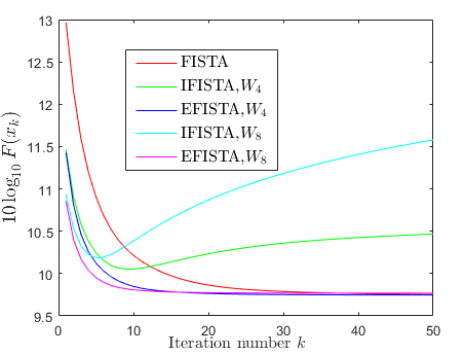
Figure 1: objective function vs iteration number

In Test $1$, we have used the blurred Cameraman image of size $256\times 256$ with $\sigma=10^{-2}$. We have calculated the weighting matrices $W_{8}$ and $W_{4}$ as described in Eq. (7), which can easily be done using spectral decomposition. We have considered $p$ value as $8=\lambda_{max}(W_{8})$ for $W_{8}$ and $4=\lambda_{max}(W_{4})$ for $W_{4}$. We have iterated the above algorithms for $50$ number of iterations and have taken $10$ number of trials to plot the curve between the objective function value $F(x_{k})$ and iteration number $k$ in Fig. 1. In this figure, we can see that the objective function value for both EFISTA and IFISTA converges faster than FISTA. However, IFISTA starts diverging after the initial few iterations for both the weighting matrices due to noise incursion. We can notice that EFISTA starts converging after $35^{th}$ iteration and $15^{th}$ iteration for $W_{4}$ and $W_{8}$ matrices, respectively.

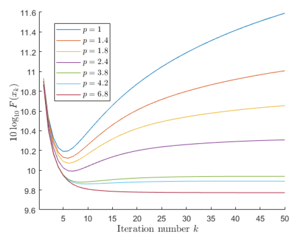
Figure 2: Objective function vs iteration number at $W_{8}$

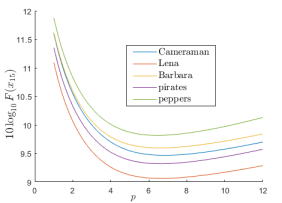
Figure 3: Objective function value at $15^{th}$ iteration vs $p$ at $W_{8}$ for different test image

In Test $2$, we repeat Test $1$ only for EFISTA with weighting matrix $W_{8}$ for different values of $p$ and plotted in Fig. 2. From this test, we observed that there is no more divergence at $p=6.8$. In Test $3$, we repeat Test $2$ of EFISTA with the same parameters for different standard test images of size $256\times 256$. The objective function value at $15^{\text{th}}$ iteration vs $p$ values is plotted in Fig. 3, which shows a clear minimization of the objective function when $p$ is closer to $\lambda_{max}(W_{8})$.

(a) Original

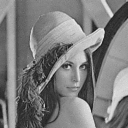
(b) FISTA

(c) IFISTA

(d) EFISTA

Figure 4: De-blurrred images for Lena test image

Noise level	Algorithms	Cameraman	Lena	Barbara	Pirate	Peppers
$\sigma=10^{-2}$	FISTA	25.39	30.21	24.34	28.30	27.50
	IFISTA	23.59	25.26	22.88	24.80	24.49
	EFISTA	25.39	30.28	24.34	28.32	27.49
$\sigma=10^{-3}$	FISTA	30.05	33.47	27.78	32.17	32.07
	IFISTA	28.79	31.06	27.24	30.43	30.13
	EFISTA	30.05	33.56	27.77	32.24	32.13

TABLE I: Average PSNR Value for different noise levels

In Test $4$, we have done deblurring of five standard test images at two noise levels, i.e., $\sigma=10^{-2}$ and $\sigma=10^{-3}$. From Test $1$ it is evident that EFISTA and IFISTA converge faster than FISTA. Therefore, in each image reconstruction, if we have used $K$ iterations for FISTA, then we have used $K/3$ iterations for both IFISTA and EFISTA. We used $K=45$ iteration for $\sigma=10^{-2}$, $K=180$ iteration for $\sigma=10^{-3}$. The PSNR values of the reconstructed images for all algorithms are presented in Table. I. We have also plotted deblurred images for noise level, $\sigma=10^{-2}$ in Fig. 4. We can notice that EFISTA performs a better reconstruction, while IFISTA incurred noise.

V Conclusion

An Enhancement Fast Iterative Shrinkage Thresholding Algorithm (EFISTA) is developed in this paper by introducing a scaled regularization term with the weighted least square term in the minimization problem. The EFISTA regulates the noise incursion effectively while taking advantage of the accelerated convergence and provides competitive image restoration performance. The simulation results confirm its superior execution speed and reconstruction quality. In the case of high AWGN, the simulation shows a better PSNR for EFISTA over IFISTA. The EFISTA Algorithm could be used as an alternative to its predecessor.

References

- [1] M. D. Daubechies and C. D. Mol, “An iterative thresholding algorithm for linear inverse problems with a sparsity constraint,” Comm. Pure Appl. Mat, no. 57, p. 1413–1457, 2004.
- [2] A. Beck and M. Teboulle, “A fast iterative shrinkage-thresholding algorithm for linear inverse problems,” SIAM journal on imaging sciences, vol. 2, no. 1, pp. 183–202, 2009.
- [3] A. Beck and M. Teboulle, “Fast gradient-based algorithms for constrained total variation image denoising and deblurring problems,” IEEE Transactions on Image Processing, vol. 18, no. 11, pp. 2419–2434, 2009.
- [4] M. Zulfiquar Ali Bhotto, M. O. Ahmad, and M. Swamy, “An improved fast iterative shrinkage thresholding algorithm for image deblurring,” SIAM journal on imaging sciences, vol. 8, no. 3, pp. 1640–1657, 2015.
- [5] M. V. Zibetti, E. S. Helou, R. R. Regatte, and G. T. Herman, “Monotone fista with variable acceleration for compressed sensing magnetic resonance imaging,” IEEE Transactions on Computational Imaging, vol. 5, no. 1, pp. 109–119, 2019.
- [6] Z. Wang, J. Wang, W. Wang, C. Gao, and S. Chen, “A novel thresholding algorithm for image deblurring beyond nesterov’s rule,” IEEE Access, vol. 6, pp. 58119–58131, 2018.
- [7] M. V. W. Zibetti, E. S. Helou, and D. R. Pipa, “Accelerating overrelaxed and monotone fast iterative shrinkage-thresholding algorithms with line search for sparse reconstructions,” IEEE Transactions on Image Processing, vol. 26, no. 7, pp. 3569–3578, 2017.
- [8] S. H. Chan, X. Wang, and O. A. Elgendy, “Plug-and-play admm for image restoration: Fixed-point convergence and applications,” IEEE Transactions on Computational Imaging, vol. 3, no. 1, pp. 84–98, 2017.
- [9] P. C. Hansen, J. G. Nagy, and D. P. O’Leary, Deblurring Images: Matrices, Spectra, and filtering, Fundam. Algorithms 3. 2006.