The Pristine Inner Galaxy Survey (PIGS) VI: Different vertical distributions between two DIBs at 442.8 nm and 862.1 nm

Abstract

Although diffuse interstellar bands (DIBs) were discovered over 100 years ago, for most of them, their origins are still unknown. Investigation on the correlations between different DIBs is an important way to study the behavior and distributions of their carriers. Based on stacking thousands of spectra from the Pristine Inner Galaxy Survey, we study the correlations between two DIBs at 442.8 nm ($\lambda$442.8) and 862.1 nm ($\lambda$862.1), as well as the dust grains, in a range of latitude spanning ${\sim}22^{\circ}$ ($4\degr\,{<}\,|b|\,{<}\,15\degr$) toward the Galactic center ($|\ell|\,{<}\,11^{\circ}$). Tight linear intensity correlations can be found between $\lambda$442.8, $\lambda$862.1, and dust grains for $|b|\,{<}\,12^{\circ}$ or $E(B\,{-}\,V)\,{>}\,0.3$ mag. For $|b|\,{>}\,12^{\circ}$, $\lambda$442.8 and $\lambda$862.1 present larger relative strength with respect to the dust grains. A systematic variation of the relative strength between $\lambda$442.8 and $\lambda$862.1 with $|b|$ and $E(B\,{-}\,V)$ concludes that the two DIBs do not share a common carrier. Furthermore, the carrier of $\lambda$862.1 is more abundant at high latitudes than that of $\lambda$442.8. This work can be treated as an example showing the significance and potentials to the DIB research covering a large latitude range.

1 Introduction

After over 100 years since the discovery of the diffuse interstellar bands (DIBs) in 1919 (Heger, 1922), over 600 DIBs have been confirmed between 0.4 and 2.4 µm (Cox et al., 2014; Galazutdinov et al., 2017b; Fan et al., 2019; Hamano et al., 2022; Ebenbichler et al., 2022). As a set of weak and broad absorption features, today DIBs are thought to be produced by carbon-bearing molecules, like carbon or hydrocarbon chains (e.g., Maier et al., 2011; Zack & Maier, 2014), polycyclic aromatic hydrocarbons (PAHs; e.g., Salama et al., 1996; Shen et al., 2018; Omont et al., 2019), and fullerenes and their derivatives (e.g., Fulara et al., 1993; Cami, 2014; Omont, 2016). However, due to the difficulties in the experimental research on complex molecules (Hardy et al., 2017; Kofman et al., 2017) and in the comparison between the experimental measurements and astronomical observations, buckminsterfullerene $(C_{60}^{+})$ is the first and only identified DIB carrier for five near-infrared DIBs so far (e.g., Foing & Ehrenfreund, 1994; Campbell et al., 2015; Walker et al., 2016; Linnartz et al., 2020), although some debates about the wavelength match and the relative strength of these bands still exist (Galazutdinov et al., 2017a; Galazutdinov et al., 2021).

Besides the comparison between astronomical observations and experimental results, investigating the correlations between different DIBs is also one of the most important ways to study the relations between their carriers and even to find the common carrier for a set of DIBs (e.g., Friedman et al., 2011; Ensor et al., 2017; Elyajouri et al., 2017; Elyajouri et al., 2018). The tightest correlation was found between two DIBs at 619.6 nm and 661.4 nm (in this work, we cite DIBs with their central wavelengths in nanometer) with very high Pearson coefficient ($r_{p}\,{>}\,0.98$; e.g., McCall et al. 2010; Friedman et al. 2011; Kos & Zwitter 2013; Bondar 2020). But the variation of their strength ratio has also been reported by Krełowski et al. (2016) and Fan et al. (2017), verifying that only a tight intensity correlation is not enough to conclude a common origin for different DIBs. The behavior of the relative strength between different DIBs as a function of $f_{\rm H_{2}}\,{\equiv}\,2N({\rm H_{2}})/[N(\text{H\,{i}})+2{N}({\rm H_{2}})]$ was used by Fan et al. (2017) to study the relative positions of the DIB carriers. Lan et al. (2015) also investigated the correlation between DIB strength and $N(\text{H\,{i}})$ and $N({\rm H_{2}})$ for 20 DIBs at high latitudes. Nevertheless, it is hard to measure $N(\text{H\,{i}})$ and $N({\rm H_{2}})$ in ultraviolet spectra or decipher the positions of H i and $\rm H_{2}$ from the radio observations. Another way is to explore the spatial distributions of different DIBs, which requires the probing of interstellar medium (ISM) above and below the Galactic plane over a large range of latitudes if we would like to get more information and conclusions from the correlation study on different DIBs. McIntosh & Webster (1993) studied the variation of the relative strength between DIBs $\lambda$442.8 , $\lambda$578.0, and $\lambda$579.7 as a function of Galactic latitudes based on a sample of 65 stars. They found the carrier abundance of $\lambda$442.8 to be highest at low latitudes, which agrees with our results (see Sect. 5.2).

The DIB research benefits from the arrival of large spectroscopic surveys allowing to perform large statistically studies. The three-dimensional (3D) distributions of the DIB carriers have been mapped by Kos et al. (2014) and Gaia collaboration, Schultheis et al. (2022) for DIB $\lambda$862.1 (we take here its central wavelength as 862.086 nm measured in Gaia collaboration, Schultheis et al. 2022), and Zasowski et al. (2015) for DIB $\lambda$1527.3, based on the data from the Radial Velocity Experiment (RAVE; Steinmetz et al., 2006), Gaia–DR3 (Gaia collaboration, Vallenari et al., 2022), and the Apache Point Observatory Galactic Evolution Experiment (APOGEE; Majewski et al., 2017), respectively. Zasowski et al. (2015), Zhao et al. (2021b), and Gaia collaboration, Schultheis et al. (2022) made preliminary studies on the kinematics of the DIB carriers with the APOGEE, Gaia–ESO (Gilmore et al., 2012), and Gaia data sets. Nevertheless, the individual spectra in large spectroscopic surveys usually have less integral time than specifically designed DIB observations, resulting in a lower signal-to-noise ratio ($\rm S/N$). Taking this into account, stacking spectra in an arbitrary spatial volume is a practical and useful method to achieve better $\rm S/N$ and to precisely measure DIB features (e.g., Kos et al., 2013; Lan et al., 2015; Baron et al., 2015a, b).

Based on the survey data, some studies devoted to the investigation on the intensity correlations between different DIBs. Elyajouri et al. (2017) made use of $\sim$300 spectra of early-type stars in APOGEE to explore the correlations between the strong DIB at 1.5273 µm and the three weak DIBs at 1.5627, 1.5653, and 1.5673 µm. A comparison between the DIB at 1.5273 µm and some optical DIBs was done as well. Based on 250 stacked spectra at high latitudes, Baron et al. (2015b) successfully clustered 26 weak DIBs into six groups and four of them were tightly associated with $\rm C_{2}$ or CN. A data-driven analysis was also done by Fan et al. (2022) for 54 strong DIBs measured in 25 high-quality spectra of early-type stars. And they suggested a continuous change of properties of the DIB carriers between different groups. The results of Puspitarini et al. (2015) showed a similar variation of the strength with the distance of background stars for DIBs $\lambda$661.4 and $\lambda$862.1 in a field centered at $(\ell,b)\,{=}\,(212.9^{\circ},{-}2.0^{\circ})$. But a direct comparison between $\lambda$661.4 and $\lambda$862.1 was not made.

In this work, we take advantage of the data from the metal-poor Pristine Inner Galaxy Survey (PIGS; Arentsen et al., 2020b) which contain a large number of spectra (13 235) and two strong DIBs ($\lambda$442.8 and $\lambda$862.1) in its blue-band and red-band spectra, respectively. Metal-poor stars have the advantage that the DIBs are less or not at all affected by stellar lines. We measure the two DIBs in stacked spectra and investigate their relative vertical distributions. In Sect. 2, we briefly introduce the PIGS survey. The stacking of spectra and the DIB measurements are described in Sect. 3. The results of the intensity correlations and vertical distributions of the two DIBs and dust grains are presented in Sect. 4 and discussed in Sect. 5. The main conclusions are summarized in Sect. 6.

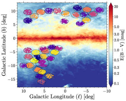
Figure 1: Spatial distribution ($\ell,b$) of 6980 PIGS targets, overplotted on the dust reddening map of Planck Collaboration et al. (2016). Colored dots represent the targets assigned into different fields (black circles), as a result of the k-means clustering with $N=36$ (see Sect. 3 for details).

2 Pristine Inner Galaxy Survey (PIGS)

The Pristine Inner Galaxy Survey (PIGS; Arentsen et al., 2020b, a, 2021) is an extension of the Pristine survey, which uses the metallicity-sensitive narrow-band $CaHK$ filter on the Canada-France-Hawaii-Telescope (CFHT) to search for and study the most metal-poor stars (Starkenburg et al., 2017). PIGS aims at obtaining spectra for the metal-poor stars in the Galactic bulge and studying their kinematics (Arentsen et al., 2020a), as well as the chemical and dynamical evolution of the inner Galaxy (Arentsen et al., 2020b, 2021; Sestito et al., 2022). The PIGS targets were selected with a magnitude limit of $13.5\,{<}\,G\,{<}\,16.5$ mag for Gaia (Gaia Collaboration et al., 2018) or $14.0\,{<}\,g\,{<}\,17.0$ mag for Pan–STARRS1 (Chambers et al., 2016), and an reddening limit of $E(B\,{-}\,V)\,{\lesssim}\,0.7$ mag from Green et al. (2018). Most of these targets (88%) have $\rm[Fe/H]\,{<}\,{-}1.0$ dex, with a peak around –1.5 dex and a tail down to –3.0 dex (Arentsen et al., 2020b). The targets were observed with AAOmega+2dF on the AAT, obtaining simultaneous blue-band (370–550 nm, $R\,{\sim}\,1300$) and red-band (840–880 nm, $R\,{\sim}\,11\,000$) spectra.

The spectra were analyzed with the FERRE code, which simultaneously derived effective temperatures, surface gravities, metallicities, and carbon abundances. For details on the analysis, see Arentsen et al. (2020b). In the original analysis, both the observed and model spectra were normalized using a running mean. For this work, we perform a re-normalization of the original observed and best-fitting synthetic spectra using the fit-continuum task in the Python specutils package. A third and fifth order Chebyshev polynomial was used for red-band and blue-band spectra, respectively.

There are 13 235 PIGS spectra observed between 2017 and 2020, of which we make use of 6980 of them, distributed into 36 fields (see Fig. 1), with $\rm S/N\,{>}\,50$ measured between 840–880 nm and $T_{\rm eff}\,{<}\,7000$ K, which assures the quality of the observed and synthetic spectra. For this subsample, $\rm S/N$ is mostly below 150 per pixel for red-band (computed between 840–880 nm) with a mean of 77, and below 50 per pixel for blue-band (computed between 400–410 nm) with a mean of 30. Thus, in this work, we only fit and measure two strong DIBs, $\lambda$442.8 and $\lambda$862.1, in stacked blue-band and red-band spectra, respectively, due to the low $\rm S/N$ of individual PIGS spectra. We applied a simple k-means algorithm (Lloyd, 1982) to cluster targets into different fields to avoid the possible overlap of observed PIGS fields, especially in the southern footprint, and to have a cleaner selection of target stars in the same $(\ell,\,b)$ range, because an overlap of fields would smooth the variation of dust reddening and DIB strength with $(\ell,\,b)$. In some cases it is also helpful for fields with worse quality spectra, to have a larger number of stars, such as the field at $(\ell_{0},\,b_{0})=(9.91^{\circ},\,{-}10.11^{\circ})$. The clustering was completed by the Python scikit-learn package (Pedregosa et al., 2011) with $N=36$, and the result is shown in Fig. 1. In the following analysis, the PIGS “fields” refer to the assigned clustered regions, which follow but are not exactly the same as their observational footprints. Discrete footprints are well clustered (e.g., the targets at $5^{\circ}\,{<}\,b\,{<}\,12^{\circ}$), while in crowded regions, such as the targets around $(\ell,\,b)=(5^{\circ},\,{-}8^{\circ})$, the clustered fields may be different from the observational ones. The central coordinates $(\ell_{0},b_{0})$, radius, and target number of each field are listed in Table 1.

Table 1: Field information and fitting results of DIB $\lambda$442.8 in the blue-band stacked ISM spectra.

Field	$\ell_{0}$	$b_{0}$	radius	$N^{a}$	$E(B\,{-}\,V)^{b}$	$\rm S/N^{c}$	$\lambda_{C}^{d}\pm{\rm err}$	$\rm FWHM^{e}\pm{\rm err}^{e}$	$\rm EW_{fit}^{f}\pm err$
Nr	(∘)	(∘)	(∘)		(mag)		(nm)	(nm)	(Å)
1	6.66	–7.15	1.14	259	$0.37\pm 0.05$	145.5	$442.76^{+0.08}_{-0.08}$	$1.99^{+0.18}_{-0.16}$	$1.10\pm 0.08$
2	–2.94	11.04	1.09	257	$0.31\pm 0.05$	104.7	$442.71^{+0.10}_{-0.09}$	$2.01^{+0.18}_{-0.18}$	$0.93\pm 0.09$
3	8.96	6.37	1.10	236	$0.57\pm 0.09$	119.0	$442.79^{+0.07}_{-0.08}$	$1.83^{+0.16}_{-0.16}$	$1.53\pm 0.09$
4	6.20	–13.97	1.00	196	$0.14\pm 0.02$	119.7	$442.54^{+0.10}_{-0.10}$	$2.07^{+0.18}_{-0.18}$	$0.73\pm 0.10$
5	3.22	–3.30	0.98	224	$0.66\pm 0.10$	89.7	$442.68^{+0.08}_{-0.08}$	$2.18^{+0.18}_{-0.18}$	$1.98\pm 0.16$
6	–4.59	8.63	1.00	104	$0.26\pm 0.06$	101.7	$442.53^{+0.10}_{-0.10}$	$2.23^{+0.20}_{-0.18}$	$0.99\pm 0.11$
7	3.86	10.00	1.09	135	$0.40\pm 0.10$	93.5	$442.77^{+0.09}_{-0.09}$	$2.03^{+0.18}_{-0.16}$	$1.13\pm 0.10$
8	–3.64	5.29	1.02	180	$0.68\pm 0.09$	112.6	$442.73^{+0.08}_{-0.08}$	$2.08^{+0.16}_{-0.16}$	$1.84\pm 0.10$
9	9.91	–10.11	1.11	99	$0.32\pm 0.07$	141.4	$442.71^{+0.09}_{-0.09}$	$2.40^{+0.20}_{-0.18}$	$1.13\pm 0.09$
10	–8.22	10.31	1.11	185	$0.29\pm 0.04$	122.5	$442.52^{+0.09}_{-0.09}$	$2.00^{+0.18}_{-0.18}$	$0.92\pm 0.09$
11	3.53	–7.45	0.95	203	$0.33\pm 0.03$	128.8	$442.65^{+0.09}_{-0.08}$	$2.12^{+0.18}_{-0.18}$	$1.25\pm 0.12$
12	0.22	6.16	0.98	225	$0.75\pm 0.07$	105.7	$442.81^{+0.07}_{-0.07}$	$1.97^{+0.16}_{-0.16}$	$2.11\pm 0.12$
13	5.51	–9.18	1.61	292	$0.27\pm 0.07$	133.7	$442.74^{+0.08}_{-0.08}$	$1.93^{+0.18}_{-0.18}$	$1.23\pm 0.09$
14	5.32	–3.97	1.09	249	$0.70\pm 0.10$	117.4	$442.75^{+0.07}_{-0.07}$	$2.10^{+0.16}_{-0.16}$	$2.01\pm 0.10$
15	8.93	9.50	1.06	182	$0.39\pm 0.04$	126.2	$442.66^{+0.09}_{-0.09}$	$2.05^{+0.18}_{-0.16}$	$1.24\pm 0.09$
16	9.00	–4.50	0.99	183	$0.61\pm 0.11$	98.2	$442.72^{+0.09}_{-0.09}$	$2.26^{+0.18}_{-0.18}$	$1.77\pm 0.12$
17	1.76	9.98	1.18	146	$0.59\pm 0.16$	122.3	$442.82^{+0.08}_{-0.09}$	$2.05^{+0.18}_{-0.18}$	$1.20\pm 0.10$
18	8.91	–6.86	1.04	130	$0.39\pm 0.08$	133.4	$442.68^{+0.09}_{-0.09}$	$2.13^{+0.18}_{-0.16}$	$1.35\pm 0.10$
19	–5.27	10.50	1.05	212	$0.25\pm 0.03$	121.7	$442.65^{+0.10}_{-0.10}$	$1.86^{+0.18}_{-0.18}$	$0.72\pm 0.08$
20	5.87	9.60	1.08	238	$0.53\pm 0.18$	127.7	$442.68^{+0.08}_{-0.08}$	$2.14^{+0.18}_{-0.16}$	$1.40\pm 0.11$
21	8.58	–10.02	1.06	250	$0.36\pm 0.06$	130.4	$442.72^{+0.09}_{-0.09}$	$1.95^{+0.18}_{-0.18}$	$0.95\pm 0.06$
22	7.42	8.06	1.06	104	$0.46\pm 0.10$	112.3	$442.74^{+0.09}_{-0.09}$	$1.94^{+0.16}_{-0.16}$	$1.33\pm 0.09$
23	–0.14	8.98	1.10	136	$0.52\pm 0.12$	120.6	$442.71^{+0.08}_{-0.08}$	$1.97^{+0.18}_{-0.16}$	$1.49\pm 0.10$
24	–5.09	6.64	1.06	177	$0.42\pm 0.12$	121.9	$442.67^{+0.08}_{-0.09}$	$2.18^{+0.18}_{-0.18}$	$1.31\pm 0.10$
25	5.12	–6.68	1.08	151	$0.35\pm 0.05$	128.1	$442.66^{+0.09}_{-0.09}$	$1.97^{+0.18}_{-0.16}$	$1.22\pm 0.09$
26	5.54	–12.41	0.98	185	$0.15\pm 0.02$	135.8	$442.62^{+0.09}_{-0.10}$	$1.98^{+0.18}_{-0.18}$	$0.74\pm 0.07$
27	2.47	–5.12	1.06	279	$0.40\pm 0.08$	140.5	$442.78^{+0.08}_{-0.08}$	$2.24^{+0.18}_{-0.16}$	$1.54\pm 0.09$
28	7.06	–5.25	1.04	179	$0.54\pm 0.06$	102.4	$442.68^{+0.08}_{-0.08}$	$2.25^{+0.18}_{-0.18}$	$1.71\pm 0.13$
29	7.39	–8.16	1.07	289	$0.37\pm 0.09$	139.7	$442.80^{+0.08}_{-0.08}$	$1.92^{+0.18}_{-0.16}$	$1.14\pm 0.07$
a The number of spectra used for stacking in each field.
b Median $E(B\,{-}\,V)$ $\pm$ its standard deviation in each field derived from the Planck map.
c Signal-to-noise ratio of the stacked blue-band ISM spectra.
d Measured central wavelength in the heliocentric frame.
e Full width at half maximum of DIB $\lambda$442.8.
f Fitted equivalent width of DIB $\lambda$442.8.

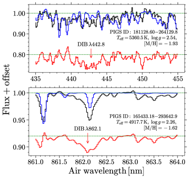
Figure 2: Two examples showing the DIB signals of $\lambda$442.8 (upper panel) and $\lambda$862.1 (lower panel) in their ISM spectra, respectively, derived by the observed blue-band and red-band PIGS spectra (black lines) and the corresponding synthetic spectra (blue lines). The DIB positions are marked. The PIGS ID and stellar atmospheric parameters of the two background stars are indicated as well.

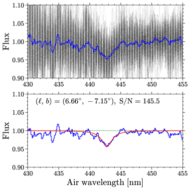
Figure 3: Upper panel: Example of stacking ISM spectra in the field $\left(\ell_{0},b_{0}\right)=\left(6.66^{\circ},{-}7.15^{\circ}\right)$. Black lines are individual ISM spectra, and the blue line is the stacked ISM spectrum. Lower panel: Fit of DIB $\lambda$442.8 in the stacked ISM spectrum after local renormalization (blue line). The red line shows the fitted Lorentzian profile. Field position and $\rm S/N$ of the stacked ISM spectrum are indicated.

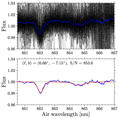
Figure 4: The same as Fig. 3, but for DIB $\lambda$862.1.

3 Fit and measure DIBs in stacked spectra

Limited by the PIGS sample size and the low S/N of individual spectra, we choose to stack spectra in each field according to their Galactic coordinates $(\ell,b)$ without taking the stellar distance into account. Thus the DIB measured in the stacked spectra is a measure of the average column density of its carrier toward a given sightline.

Before stacking spectra in each field, the stellar components in observed spectra are first subtracted by the synthetic spectra, providing the ISM spectra for each target. Figure 2 shows two ISM spectra derived from the blue-band and red-band observed spectra, respectively, subtracted by their synthetic spectra. The DIB signals are clear, although their profiles are contaminated by noise and the residuals of stellar lines, such as the Fe i line close to the center of $\lambda$862.1. We emphasize that in the stacked ISM spectra these contamination are significantly alleviated (see Figs. 3 and 4) due to the averaging of a substantial number of spectra and the large velocity dispersion of stars in each field (standard deviation ${>}100\,\rm km\,s^{-1}$). The second step is to shift the ISM spectra back to the heliocentric frame using the stellar radial velocities (${\rm RV_{star}}$, in $\rm km\,s^{-1}$), that is $\lambda_{\rm pixel}^{\prime}=\lambda_{\rm pixel}+{\rm RV_{star}}\times\lambda_{\rm pixel}/c$, where $\lambda_{\rm pixel}^{\prime}$ and $\lambda_{\rm pixel}$ are the wavelength pixels in the heliocentric and stellar frames, respectively, and $c\,{=}\,3\,{\times}\,10^{5}\,\rm km\,s^{-1}$ is the speed of light. Finally, stacking of individual ISM spectra in each field is done for the blue band and red band, respectively, by taking the median value of their flux which could reduce the influence of the outlier pixels and discrepancy between the individual observed and synthetic spectra. A $\rm S/N$ is calculated between 860.5 and 861.5 nm for red-band stacked ISM spectra by $\rm mean(flux)/std(flux)$. For blue-band stacked ISM spectra, fluxes are used in two windows, that is 430–433 nm and 452–455 nm. Examples for blue-band and red-band stacked ISM spectra can be found in the upper panels in Figs. 3 and 4, respectively. The $\rm S/N$ of stacked spectra (listed in Tables 1 and 2) are dramatically increased.

Compared to the red band, the blue-band stacked ISM spectra are more noisy and have much more residual features with stellar origins. This could partly be due to the abundance variations which are common at low metallicity. Thus, fitting a continuum straight through the ISM spectra could lead to an underestimation of the strength of $\lambda$442.8. Therefore, we apply the Gaussian process regression (GPR; Gershman & Blei, 2012; Rasmussen & Williams, 2006) to fit the profile of $\lambda$442.8, the stellar residuals, and the random noise simultaneously. This method has been successfully applied to the spectra of early-type stars (Kos, 2017; Zhao et al., 2021a). Specifically, the blue-band stacked ISM spectra are first locally renormalized with the spectral window of 430–455 nm by an iterated method using a second-order polynomial (see Sect. 2.2 in Zhao et al. 2021a for details). Then the ISM spectra are initially fitted by a Lorentzian function for the profile of $\lambda$442.8, as suggested by Snow et al. (2002), and a constant continuum. Finally, GPR is applied with a Lorentzian function as its mean function and a Matérn 3/2 kernel to model the correlated noise, including both the stellar residuals and random noise. Only one kernel is used here because DIB $\lambda$442.8 is the broadest feature in the ISM spectra. The priors of fitting parameters mainly follow those in Kos (2017) and Zhao et al. (2021a), that is Gaussian priors centered at the initial fitting results with a width of 0.15 nm for the DIB central wavelength and the Lorentzian width and a flat prior for the scale length of the Matérn 3/2 kernel. Details about GPR and the priors can be found in Kos (2017) and Zhao et al. (2021a).

The stellar residuals are much less in the red-band stacked ISM spectra. Among them, the strongest one is from the Ca ii line around 866.5 nm. But it is far away from the DIB $\lambda$862.1. Using stacked Gaia–RVS spectra (Gaia collaboration, Seabroke et al., 2022), Zhao et al. (2022) confirmed that the weak DIB around 864.8 nm is very broad, with a Full Width at Half Maximum (FWHM) of $\sim$1.6 nm, and its profile could affect the placement of the continuum (see Fig. 1 in Zhao et al. 2022). Therefore, we fit each red-band stacked ISM spectrum between 860.5 and 867 nm with a Gaussian function for the profile of $\lambda$862.1, a Lorentzian function for the profile of $\lambda$864.8, and a linear continuum. Nevertheless, the DIB $\lambda$864.8 profile cannot be well described due to the lower quality of the individual ISM spectra at longer wavelength (see upper panel in Fig. 4). We emphasize that because DIBs are absorption features, the usage of the whole spectra between 860.5 and 867 nm can help us to get a better placement of the continuum, although the $\lambda$864.8 profile cannot be well fitted.

The parameter optimization, for both red band and blue band, is implemented by a Markov Chain Monte Carlo (MCMC) procedure (Foreman-Mackey et al., 2013). The 50% values in the posterior distribution generated by MCMC are treated as the best estimates, with lower and upper errors derived from the differences of 16% and 84% to 50% values, respectively. Fit examples of $\lambda$442.8 and $\lambda$862.1 are shown in Figs. 3 and 4, respectively.

Table 2: Fitting results of DIB $\lambda$862.1 in the red-band stacked ISM spectra. The field numbers are the same as Table 1.

Field	$\rm S/N^{a}$	$\lambda_{C}^{b}\pm{\rm err}$	$\rm FWHM^{c}\pm err$	$\rm EW_{fit}^{d}\pm err$	$\rm EW_{int}^{e}$
Nr		(nm)	(nm)	(Å)	(Å)
1	853.6	$862.06^{+0.02}_{-0.02}$	$0.45^{+0.06}_{-0.05}$	$0.088\pm 0.004$	0.091
2	555.0	$862.07^{+0.02}_{-0.02}$	$0.46^{+0.06}_{-0.05}$	$0.091\pm 0.003$	0.093
3	756.1	$862.06^{+0.02}_{-0.02}$	$0.48^{+0.05}_{-0.05}$	$0.157\pm 0.006$	0.159
4	996.9	$862.06^{+0.03}_{-0.02}$	$0.56^{+0.08}_{-0.07}$	$0.105\pm 0.006$	0.107
5	529.5	$862.06^{+0.02}_{-0.02}$	$0.47^{+0.05}_{-0.04}$	$0.189\pm 0.004$	0.190
6	519.3	$862.04^{+0.03}_{-0.03}$	$0.46^{+0.08}_{-0.07}$	$0.085\pm 0.005$	0.091
7	930.8	$862.06^{+0.02}_{-0.02}$	$0.47^{+0.05}_{-0.05}$	$0.105\pm 0.004$	0.111
8	595.4	$862.04^{+0.02}_{-0.02}$	$0.46^{+0.05}_{-0.05}$	$0.187\pm 0.005$	0.191
9	447.1	$862.05^{+0.03}_{-0.03}$	$0.42^{+0.07}_{-0.06}$	$0.071\pm 0.004$	0.072
10	583.6	$861.96^{+0.02}_{-0.02}$	$0.48^{+0.06}_{-0.05}$	$0.094\pm 0.004$	0.093
11	722.8	$862.08^{+0.02}_{-0.02}$	$0.48^{+0.06}_{-0.06}$	$0.109\pm 0.005$	0.112
12	563.9	$862.05^{+0.01}_{-0.01}$	$0.46^{+0.03}_{-0.03}$	$0.220\pm 0.007$	0.227
13	780.2	$862.07^{+0.02}_{-0.02}$	$0.46^{+0.05}_{-0.04}$	$0.140\pm 0.004$	0.145
14	754.3	$862.07^{+0.01}_{-0.01}$	$0.47^{+0.03}_{-0.03}$	$0.199\pm 0.005$	0.203
15	740.9	$862.04^{+0.02}_{-0.02}$	$0.49^{+0.05}_{-0.05}$	$0.123\pm 0.004$	0.127
16	719.3	$862.09^{+0.02}_{-0.02}$	$0.47^{+0.04}_{-0.04}$	$0.170\pm 0.007$	0.172
17	868.2	$862.06^{+0.02}_{-0.02}$	$0.48^{+0.07}_{-0.06}$	$0.103\pm 0.007$	0.111
18	830.6	$862.08^{+0.02}_{-0.02}$	$0.45^{+0.06}_{-0.05}$	$0.100\pm 0.004$	0.102
19	579.6	$862.07^{+0.02}_{-0.02}$	$0.48^{+0.07}_{-0.06}$	$0.084\pm 0.004$	0.087
20	944.7	$862.06^{+0.02}_{-0.02}$	$0.49^{+0.05}_{-0.04}$	$0.129\pm 0.004$	0.135
21	915.9	$862.06^{+0.02}_{-0.02}$	$0.48^{+0.06}_{-0.05}$	$0.090\pm 0.003$	0.094
22	730.9	$862.06^{+0.01}_{-0.02}$	$0.46^{+0.04}_{-0.04}$	$0.124\pm 0.006$	0.127
23	886.1	$862.07^{+0.02}_{-0.02}$	$0.50^{+0.06}_{-0.05}$	$0.140\pm 0.007$	0.147
24	589.3	$862.04^{+0.02}_{-0.02}$	$0.46^{+0.05}_{-0.04}$	$0.114\pm 0.004$	0.117
25	882.8	$862.07^{+0.02}_{-0.02}$	$0.45^{+0.07}_{-0.06}$	$0.113\pm 0.006$	0.116
26	674.8	$862.05^{+0.02}_{-0.02}$	$0.52^{+0.08}_{-0.07}$	$0.100\pm 0.005$	0.105
27	627.4	$862.07^{+0.02}_{-0.02}$	$0.47^{+0.06}_{-0.05}$	$0.133\pm 0.003$	0.134
28	491.1	$862.06^{+0.02}_{-0.02}$	$0.49^{+0.07}_{-0.06}$	$0.137\pm 0.005$	0.142
29	547.3	$862.05^{+0.02}_{-0.02}$	$0.42^{+0.04}_{-0.04}$	$0.102\pm 0.004$	0.101
a Signal-to-noise ratio of the red-band stacked ISM spectra.
b Measured central wavelength in the heliocentric frame.
c Full width at half maximum of DIB $\lambda$862.1.
d Fitted equivalent width of DIB $\lambda$862.1.
e Integrated equivalent width of DIB $\lambda$862.1.

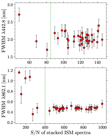
Figure 5: FHWM versus $\rm S/N$ of stacked ISM spectra for DIBs $\lambda$442.8 (upper panel) and $\lambda$862.1 (lower panel). The dashed green lines indicate $\rm S/N=85$ and 400, respectively.

4 Result

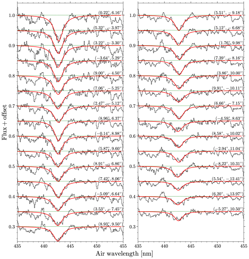
Figure 13: Fits of $\lambda$442.8 in blue-band stacked ISM spectra. The black lines are the stacked ISM spectra, and the red lines are the fitted DIB profile. The results are sorted by the measured $\rm EW_{442.8}$. The Galactic coordinates $(\ell,b)$ of each field are also indicated.

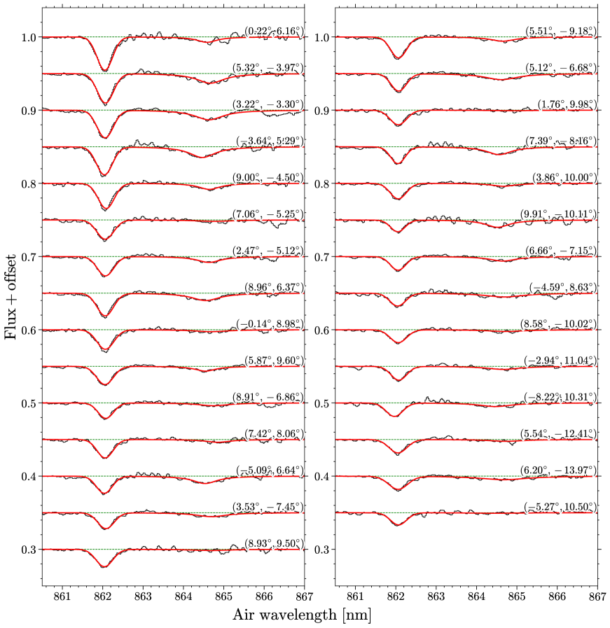
Figure 14: The same as Fig. 13, but for DIB $\lambda$862.1.

The goodness of fit is significantly affected by the $\rm S/N$ of the stacked ISM spectra. Figure 5 shows the $\rm S/N$ of each stacked ISM spectrum versus the corresponding fitted FWHMs of DIBs $\lambda$442.8 and $\lambda$862.1. It can be seen that in the spectra with low $\rm S/N$, the fitted FWHM could be much larger than the average value and/or have much larger uncertainties than average. Therefore, we limit $\rm S/N\,{>}\,85$ and $\rm S/N\,{>}\,400$ for blue-band and red-band stacked ISM spectra, respectively, which gives us 29 fields with reliable fitting results of the two DIBs. Further analysis is based on this sample. The stacked ISM spectra and fits to the two DIBs are shown in Figs. 13 and 14, respectively. The measured central wavelength, FWHM, and fitted equivalent width (EW) of the two DIBs $\lambda$442.8 and $\lambda$862.1 are listed in Tables 1 and 2, respectively. The EW uncertainty is calculated as ${\rm\Delta EW}\,{=}\,\sqrt{6\,{\rm FWHM}\,\delta\lambda}\times{\it R_{C}}$, where $\delta\lambda$ is the spectral pixel resolution (0.1 nm for blue-band and 0.025 nm for red-band) and $R_{C}\,{=}\,{\rm std(data-model)}$ is the noise level of the profile. This formula is similar to those in Vos et al. (2011) and Vollmann & Eversberg (2006), who considered the main source of EW uncertainty as S/N and the placement of the continuum. ${\rm EW_{442.8}}$ has larger uncertainties than that of ${\rm EW_{862.1}}$ due to the lower $\rm S/N$ of the blue band than that of the red band.

The integrated EW of $\lambda$862.1 is also calculated and listed in Table 2. This is not done for $\lambda$442.8 because of the stellar residuals within the DIB profile. The comparison between fitted and integrated $\rm EW_{862.1}$ is presented in Fig 6. The EW difference is on average smaller than its uncertainty. But the integrated EW tends to be slightly larger than the fitted EW, which could be caused by the residuals of stellar lines near the DIB or the potential asymmetry of the DIB profile. The fitted ${\rm EW_{442.8}}$ and ${\rm EW_{862.1}}$ are used for following analysis.

The average FWHM of $\lambda$442.8 measured in this work is $2.06\,{\pm}\,0.13$ nm, which is slightly larger than the report in Snow et al. (2002, 1.725 nm). Lai et al. (2020) attributed the wide range of FWHM values of $\lambda$442.8 in literature (e.g., 1.7 nm in Galazutdinov et al. 2020; 2.4 nm in Fan et al. 2019; 3.37 nm in Lai et al. 2020) to the differences in the local radiation field. The average FWHM of $\lambda$862.1 measured in this work is $0.47\,{\pm}\,0.03$ nm, which is close to the measure of 0.43 nm in Herbig & Leka (1991) and 0.469 nm in Maíz Apellániz (2015).

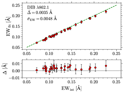
Figure 6: Upper panel: Comparison between integrated and fitted EW for DIB $\lambda$862.1. The dashed green line traces the one-to-one correspondence. The average difference between integrated and fitted EW ($\rm\Delta=EW_{int}-EW_{fit}$) and the mean EW uncertainty ($\rm\bar{\sigma}_{EW}$) are indicated. Lower panel: The EW differences as a function of the integrated EW. The dashed black line marks a zero difference.

4.1 Latitude groups

In this work, we derive $E(B\,{-}\,V)$ for each PIGS target from the map of Planck Collaboration et al. (2016) using the python package dustmaps (Green, 2018) because these target stars are mainly very distant and at high latitudes ($93.6\%$ with $|b|\,{>}\,4^{\circ}$). The median $E(B\,{-}\,V)$ in each PIGS field, together with its standard deviation as a measure of uncertainty, are listed in Table 1. To check the reliability of the Planck map for PIGS targets, we compare the reddening values with estimates from two other sources: the 3D reddening values derived with the StarHorse algorithm (Queiroz et al., 2018) specifically for the PIGS stars using the PIGS spectroscopic stellar parameters, Pan–STARRS1 photometry, and Gaia parallaxes (Arentsen et al. in prep.), and the 3D Bayestar reddening map (Green et al., 2019) applying the StarHorse distances. The usage of PIGS stellar parameters into StarHorse delivers a more constrained and less uncertain reddening and distances than those from the StarHorse Gaia database (Anders et al., 2022) for the same stars, but that only used photometry and parallaxes as input. About 80% PIGS target stars have StarHorse and Bayestar $E(B\,{-}\,V)$, among which, 90% stars are further than 5 kpc. The comparison between the Planck, StarHorse, and Bayestar reddenings is presented in Fig. 7. $E(B\,{-}\,V)$ from Planck and StarHorse are highly consistent with each other (the mean difference is smaller than one thousandth magnitude), while the Bayestar $E(B\,{-}\,V)$ is slightly larger (0.033 mag on average) than the Planck values, which could be due to the different methods of reddening inference. The differences of median $E(B\,{-}\,V)$ in the 29 used PIGS fields (red squares in Fig. 7) between Planck, StarHorse, and Bayestar are mostly smaller than their uncertainties. This ensures that the usage of Planck $E(B\,{-}\,V)$, which can be derived for all the PIGS targets, can be a safe measure of the dust column densities toward these sightlines.

In our sample, $E(B\,{-}\,V)$ is strongly correlated with the Galactic latitude. Thus, the PIGS fields are divided into three latitude stripes to highlight the effect of latitude in the following analysis. The middle stripe is further separated into two at $\ell\,{=}\,{-}1^{\circ}$ considering the effect of $\ell$ toward the Galactic center (GC). Finally, we roughly define four latitude groups (see Fig. 8): G1: $|b|\,{>}\,12^{\circ}$ (red), G2: $8^{\circ}\,{<}\,|b|\,{<}\,12^{\circ}$ and $\ell\,{>}\,{-}1^{\circ}$ (yellow), G3: $8^{\circ}\,{<}\,|b|\,{<}\,12^{\circ}$ and $\ell\,{<}\,{-}1^{\circ}$ (cyan), and G4: $|b|\,{<}\,8^{\circ}$ (blue).

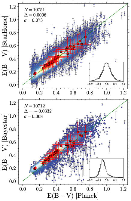
Figure 7: Comparison of $E(B\,{-}\,V)$ derived from Planck Collaboration et al. (2016) with those from the StarHorse algorithm (upper panel) and from the Bayestar map (lower panel). The colored dots with uncertainties are for individual PIGS target stars. Their colors represent the number densities estimated by a Gaussian kernel density estimation. The zoom-in panels show the $E(B\,{-}\,V)$ differences of Planck–StarHorse and Planck–Bayestar, respectively. The number of PIGS target stars ($N$), the mean differences ($\Delta$), and its standard deviation ($\sigma$) are indicated in the panels. The red squares with errorbars are the median $E(B\,{-}\,V)$ and their standard deviations calculate in 29 used PIGS fields. The dashed green lines trace the one-to-one correspondence.

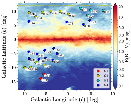
Figure 8: Spatial distribution $(\ell,b)$ of 29 PIGS fields, overplotted on the dust reddening map of Planck Collaboration et al. (2016). Different colors indicate different latitude groups defined in Sect. 4.1, that is red: G1, $|b|\,{>}\,12^{\circ}$; yellow: G2, $8^{\circ}\,{<}\,|b|\,{<}\,12^{\circ}$ and $\ell\,{>}\,{-}1^{\circ}$; cyan: G3, $8^{\circ}\,{<}\,|b|\,{<}\,12^{\circ}$ and $\ell\,{<}\,{-}1^{\circ}$, and blue: G4, $|b|\,{<}\,8^{\circ}$. The median $E(B\,{-}\,V)$ of each filed is also indicated.

4.2 Linear relations between different interstellar materials

One of the basic characteristics of most strong DIBs is the increase of their strength with dust reddenings. Figure 9 shows the correlation between DIB strength ($\rm EW_{442.8}$ and $\rm EW_{862.1}$) and $E(B\,{-}\,V)$. Linear correlation with $E(B\,{-}\,V)$ can be found for both $\lambda$442.8 and $\lambda$862.1 with a Pearson coefficient of $r_{p}\,{=}\,0.92$ and $r_{p}\,{=}\,0.83$, respectively. The two outliers in G2 (yellow points) are due to the local variation of $E(B\,{-}\,V)$, that one with $E(B\,{-}\,V)\,{=}\,0.59$ mag is higher than its vicinity and the other with $E(B\,{-}\,V)\,{=}\,0.27$ mag is lower than its neighboring values (see Fig. 8). Deviations from the linear correlation between DIB and $E(B\,{-}\,V)$ can also be found at high latitudes (see red points in Fig. 9), which will be discussed in detail below. A linear fit of $E(B\,{-}\,V)=0.363(\pm 0.041)\times{\rm EW_{442.8}}-0.048(\pm 0.051)$ corresponds to ${\rm EW_{442.8}}/E(B\,{-}\,V)\,{=}\,2.75$ Å mag^-1, which is in the intermediate range compared to the results in literature (e.g., 2.89 of Isobe et al. 1986 and 2.01 of Fan et al. 2019). For $\lambda$862.1, we derived a coefficient of $E(B\,{-}\,V)/{\rm EW_{862.1}}\,{=}\,3.500\pm 0.459$ mag Å^-1 with a very small intercept (${-}0.007\pm 0.059$). This value is slightly larger than previous results (e.g., Munari et al., 2008; Kos et al., 2013; Krełowski et al., 2019) but between the values derived from Gaia–DR3 DIB results with different $E(B\,{-}\,V)$ sources (see Table 3 in Gaia collaboration, Schultheis et al., 2022).

It has been known that the ratio of $E(B\,{-}\,V)/{\rm EW}$ can vary significantly from one sightline to another and is also affected by the use of different data samples and methods. Nevertheless, we argue that the positive correlation between DIB strength and dust reddening in diffuse or intermediate ISM with a proper coefficient can be treated as a validation of the DIB measurement. For our results, the range of $\rm EW_{442.8}$ at given $E(B\,{-}\,V)$ between 0.2 and 0.8 mag is consistent with archival data shown in Fig. 5 in Lai et al. (2020) and early results of Herbig (1975) shown in Fig. 6 in Snow et al. (2002). The variation of $\rm EW_{862.1}$ relative to $E(B\,{-}\,V)$ is also within the regions, considering the scatter, shown in Fig. 8 in Gaia collaboration, Schultheis et al. (2022).

The tight linear correlation ($r_{p}\,{=}\,0.94$) between the DIB strength of $\lambda$442.8 and $\lambda$862.1 can be seen in Fig. 10 for $\rm EW_{442.8}\,{>}\,0.9$ Å. A linear fit yields $\rm EW_{862.1}/EW_{442.8}=0.098\pm 0.007$ with a very small offset of ${-}0.008\pm 0.009$. Note that the strongest DIB $\lambda$442.8 is stronger than $\lambda$862.1 by a factor of 10 for our results, which is consistent with the average of their relative strength measured in Fan et al. (2019). However, three fields with $\rm EW_{442.8}\,{<}\,0.9$ Å have $\rm EW_{862.1}$ much larger than that expected by the linear relation.

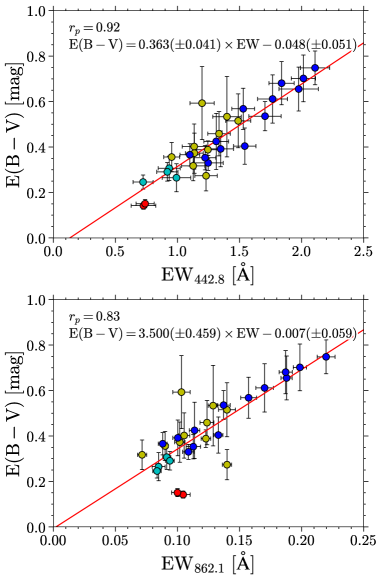
Figure 9: Correlation between DIB EW of $\lambda$442.8 (upper panel) and $\lambda$862.1 (lower panel) measured in stacked ISM spectra and median $E(B\,{-}\,V)$ from Planck map in corresponding fields. The red lines are the linear fits. The fitting results and the Pearson coefficient ($r_{p}$) are also indicated. The points in different colors belong to different latitude groups defined in Sect. 4.1 and shown in Fig. 8.

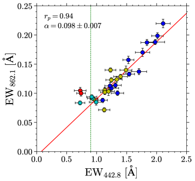
Figure 10: Correlation between $\rm EW_{442.8}$ and $\rm EW_{862.1}$ measured in blue-band and red-band stacked ISM spectra, respectively. The red line is the linear fit to the dots with $\rm EW_{442.8}>0.9$ Å (indicated by the dashed green line). The fitted slope ($\alpha$) and Pearson coefficient ($r_{p}$) are indicated. The points are colored differently according to the latitude groups they are assigned to (see Sect. 4.1 and Fig. 8).

4.3 Variation of the relative strength with Galactic latitude and reddening

The systematic variation of $\rm EW_{862.1}/EW_{442.8}$ with the Galactic latitude ($|b|$) and dust reddening ($E(B\,{-}\,V)$) are presented in the upper panels in Figs. 11 and 12, respectively, whose uncertainty considers both the contribution of $\rm EW_{862.1}$ and $\rm EW_{442.8}$ by error propagation. $\rm EW_{862.1}/EW_{442.8}$ becomes larger than average for $|b|\,{\gtrsim}\,10^{\circ}$ or $E(B\,{-}\,V)\,{\lesssim}\,0.3$ mag, where an increase of $\rm EW_{862.1}/EW_{442.8}$ can be found with the increasing $|b|$ and the decreasing $E(B\,{-}\,V)$. The uncertainty of $\rm EW_{862.1}/EW_{442.8}$ tends to be larger in the fields with high latitudes or small $E(B\,{-}\,V)$, which have a risk to blur the variation of the DIB relative strength. But we notice that for the G1 fields (red points in Figs. 11 and 12) with $E(B\,{-}\,V)\,{<}\,0.2$ mag and $|b|\,{>}\,12^{\circ}$, the increasing magnitude of their mean $\rm EW_{862.1}/EW_{442.8}$ 0.140) to the fitted coefficient (0.098) is 0.042, which is bigger than their mean uncertainty (0.018) by a factor of two. Moreover, a tight negative correlation ($r_{p}\,{=}\,{-}0.88$) can be found between $\rm EW_{862.1}/EW_{442.8}$ and $E(B\,{-}\,V)$ for $E(B\,{-}\,V)\,{<}\,0.31$ mag, which also confirms that the variation of $\rm EW_{862.1}/EW_{442.8}$ with $|b|$ and $E(B\,{-}\,V)$ is not caused by the EW uncertainty but indicates the different distributions of the carriers of the two DIBs (see Sect. 5 for more discussions). For $E(B\,{-}\,V)\,{\gtrsim}\,0.45$ mag, $\rm EW_{862.1}/EW_{442.8}$ tends to slightly increase with $E(B\,{-}\,V)$ (see top panel in Fig. 12), but more data are needed to confirm this trend. We also emphasize that in Fig. 10, three G3 fields (cyan points) with $\rm EW_{442.8}\,{>}\,0.9$ Å were used for the linear fit of DIB strength to make the offset of the line close to zero, but their $\rm EW_{862.1}/EW_{442.8}$ already present a systematic variation with respect to $E(B\,{-}\,V)$.

In our sample, fields at high latitudes in general have small $E(B\,{-}\,V)$, but the dust distribution shown in Fig 8 also varies with longitudes and sightlines. Consequently, we can find a G3 field, with $(\ell,b)\,{=}\,({-}4.59^{\circ},8.63^{\circ})$ and $E(B\,{-}\,V)\,{=}\,0.26$ mag, that follows the negative trend between $\rm EW_{862.1}/EW_{442.8}$ and $E(B\,{-}\,V)$ but does not present a clear variation of $\rm EW_{862.1}/EW_{442.8}$ with $|b|$. The non-monotonic relationship between $|b|$ and $E(B\,{-}\,V)$, as well as the averaging of ISM and the complicated environments toward the GC, also introduces the scatters in Figs. 11 and 12.

Similar pictures can also be found for ${\rm EW_{442.8}}/E(B\,{-}\,V)$ and ${\rm EW_{862.1}}/E(B\,{-}\,V)$ which are shown in the middle and lower panels in Figs. 11 and 12, respectively. A remarkable increase of ${\rm EW}/E(B\,{-}\,V)$ can be found for two G1 fields in our sample for both $\lambda$442.8 and $\lambda$862.1. ${\rm EW_{862.1}}/E(B\,{-}\,V)$ stay around the linear relation in a wide range of $|b|\,{\lesssim}\,11^{\circ}$ or $E(B\,{-}\,V)\,{\gtrsim}\,0.3$ mag. Nevertheless, ${\rm EW_{442.8}}/E(B\,{-}\,V)$ presents larger scatters with respect to $|b|$ and $E(B\,{-}\,V)$ than ${\rm EW_{862.1}}/E(B\,{-}\,V)$, which implies that the carrier abundance of $\lambda$442.8 would be more sensitive to the dust column densities and latitudes than that of $\lambda$862.1. ${\rm EW}/E(B\,{-}\,V)$ tends to be larger than average for $E(B\,{-}\,V)$ between 0.25 and 0.4 mag, but no linear tendency can be found.

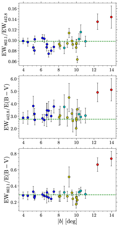
Figure 11: Variation of relative strength between DIBs $\lambda$442.8, $\lambda$862.1, and dust with Galactic latitude ($|b|$). The dashed green lines indicate their average strength ratios from linear fits (see Sect. 4.2). See Sect. 4.1 and Fig. 8 for the point colors representing different latitude groups.

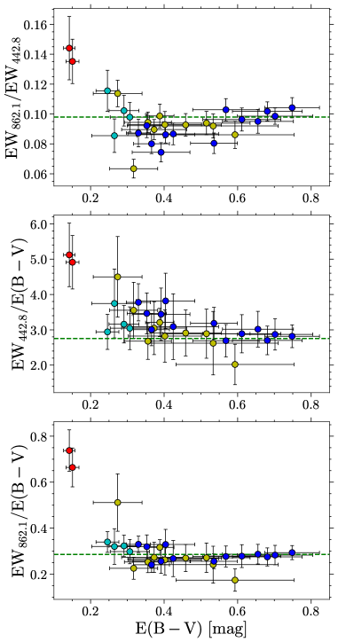
Figure 12: The same as Fig. 11, but for the variation with $E(B\,{-}\,V)$.

5 Discussion

5.1 Relative vertical distributions between DIB carriers and dust grains

By covering a wide range of Galactic latitude ($4\degr\,{<}\,|b|\,{<}\,15\degr$) and dust reddening ($0.1\,{<}\,E(B\,{-}\,V)\,{<}\,0.8$ mag), our results show that the DIBs $\lambda$442.8 and $\lambda$862.1 engage similar behavior with dust grains, that is the change of their ${\rm EW}/E(B\,{-}\,V)$ is constant and around the mean value considering the uncertainties for $|b|\,{<}\,12^{\circ}$ or $E(B\,{-}\,V)\,{>}\,0.3$ mag, which indicates that the abundance of the DIB carriers and dust grains increase with each other in the Galactic middle plane. On the other hand, ${\rm EW}/E(B\,{-}\,V)$ becomes significantly larger than average in the G1 fields at high latitudes. This phenomenon could be interpreted as an evidence that DIBs and dust grains have different vertical distributions in the Milky Way, because in our sample small $E(B\,{-}\,V)$ generally indicate sight lines towards higher latitudes. However, clearly more data especially at higher galactic latitudes are necessary to confirm the different vertical distributions between the DIBs and the dust.

For our present sample, we cannot quantitatively estimate a scale height for the DIB carrier or dust because of the limited sample size and the gaps at $|b|\,{\sim}\,12^{\circ}$ and $E(B\,{-}\,V)\,{\sim}\,0.2\,$mag. But the increase of ${\rm EW}/E(B\,{-}\,V)$ at high latitudes indicates the decrease of the column density of dust grains with respect to that of the DIB carriers, implying a larger scale height of the DIB carriers for both $\lambda$442.8 and $\lambda$862.1 than that of the dust grains if we assume a simple disk model for them and that one with a larger scale height would have a larger scale length as well. This result is consistent with the detection of DIBs toward sightlines with negligible reddenings at high latitudes (Baron et al., 2015b) and the result of Kos et al. (2014) who measured $\lambda$862.1 in RAVE spectra in a range of $240^{\circ}\,{\leqslant}\,\ell\,{\leqslant}\,330^{\circ}$. However, based on the Gaia–DR3 results, Gaia collaboration, Schultheis et al. (2022) determined a scale height of DIB $\lambda$862.1 as $98.69^{{+}10.81}_{{-}8.35}$ pc in a range of $0^{\circ}\,{\leqslant}\,{\ell}\,{\leqslant}\,360^{\circ}$ and $4^{\circ}\,{\leqslant}\,{|b|}\,{\leqslant}\,12^{\circ}$, which is smaller than the usually suggested scale height of dust grains, such as $134.4{\pm}8.5$ pc (Drimmel & Spergel, 2001) and $125^{{+}17}_{{-}7}$ pc (Marshall et al., 2006). The discrepancy could be a result of the variation of the distribution of DIB carriers and dust grains from one sightline to another (see the wavy pattern of the dust shown in Lallement et al. 2022 for example). Furthermore, the vertical distribution of interstellar materials would be more complicated than a single exponential model. Guo et al. (2021) fitted the dust distribution with a two-disk model and got two scale heights of $72.7{\pm}2.4$ pc and $224.6{\pm}0.7$ pc for the thin and thick disks. Similarly, Su et al. (2021) also characterized the molecular disk, traced by ¹²CO $J\,{=}\,(1{-}0)$ emission (Su et al., 2019), by two components with a thickness of ${\sim}85$ pc and ${\sim}280$ pc, respectively, in a range of $16^{\circ}\,{\leqslant}\,{\ell}\,{\leqslant}\,25^{\circ}$ and ${|b|}\,{<}\,5.1^{\circ}$. The Gaia result presents an average of the scale height of the carrier of $\lambda$862.1 in vicinity of the Sun ($\lesssim$3 kpc). Nevertheless, the PIGS target stars are located toward the GC ($\ell\,{<}\,11^{\circ}$) and more distant (90% $>$5 kpc) that could trace a different relative vertical distribution between DIB carriers and dust grains, if we expect their distributions vary in different manners.

5.2 Different vertical distributions between carriers of different DIBs

Tight intensity correlations have been reported for many strong optical DIBs (e.g., Friedman et al., 2011; Xiang et al., 2012; Kos & Zwitter, 2013). But most of these works rely on OB stars that mainly reside in the Galactic middle plane, where one can always get a linear relationship between different interstellar materials in a broad enough distance range. Thus, a tight linearity is a necessary but not sufficient condition to conclude a common origin for different DIBs. An example is $\lambda$578.8 and $\lambda$579.7 that they have been proved to have different origins (e.g., Krełowski & Westerlund, 1988; Cami et al., 1997; Kos & Zwitter, 2013) but high-level correlations can still be found with $r_{p}\,{>}\,0.9$ (e.g., Friedman et al., 2011; Xiang et al., 2012; Kos & Zwitter, 2013).

The variation of $\rm EW_{862.1}/EW_{442.8}$ with $|b|$ and $E(B\,{-}\,V)$ is a strong evidence that $\lambda$442.8 and $\lambda$862.1 do not share a common carrier. Moreover, their carriers could be well mixed in the fields with high reddenings or low latitudes seen though their tight intensity correlation ($r_{p}\,{=}\,0.94$). But the carrier of $\lambda$862.1 becomes more abundant with respect to $\lambda$442.8 at higher latitudes, which is consistent with McIntosh & Webster (1993) who found that the strength of $\lambda$442.8 relative to those of $\lambda$578.0 and $\lambda$5797.7 was greatest at low latitude and decreased with increasing latitude. Baron et al. (2015a) also showed that $\lambda$442.8 was absent in their spectra at high latitudes while $\lambda$578.0 and $\lambda$5797.7 tended to have higher EW per reddening. Our results are in agreement with their findings that different DIB carriers could present different vertical distributions and the carrier of $\lambda$442.8 seems to be mainly located in the Galactic plane compared to other DIBs. A different origin for $\lambda$442.8 and $\lambda$862.1 is not unexpected as they are far away from each other in wavelength and their profiles show different shapes. However, they can be treated as an example to illustrate the significance to explore the spatial distributions, especially for high-latitude regions, of different DIBs when we would like to confirm a common or different origin for them.

A potential risk of the above interpretation is the change of the environmental conditions, like temperature, from the Galactic middle plane to the regions far away from it. It is therefore possible that a single DIB carrier produces two DIBs from two different transitions that show different vertical structures. As $C_{60}^{+}$ is the only identified DIB carrier and the variation of its DIBs with environments has not been observed, it is hard to characterize this effect. Further studies, combined with other known atomic or molecular species, could address this problem to some extent. In the future, much can be gained from the large sky-area spectroscopic surveys to investigate if there exists a layered structure along the vertical direction for a set of DIBs, revealing a hierarchical distribution of various macromolecules or a dependence of their electronic transitions on the interstellar environments.

6 Conclusions

Based on stacking blue-band and red-band ISM spectra from the PIGS sample, we successfully fitted and measured two DIBs $\lambda$442.8 and $\lambda$862.1 in 29 fields with a mean radii of 1°. Their FWHM was estimated as $2.06\,{\pm}\,0.13$ nm for $\lambda$442.8 and $0.47\,{\pm}\,0.03$ nm for $\lambda$862.1, which are both consistent with previous measurements.

Our results depict a general image of the relative distributions of two DIBs and dust grains toward the GC with $|\ell|\,{<}\,11^{\circ}$ and $4\degr\,{<}\,|b|\,{<}\,15\degr$. The DIB carriers and dust grains are well mixed with each other for $|b|\,{<}\,12^{\circ}$ or $E(B\,{-}\,V)\,{>}\,0.3$ mag. Tight linear correlations are derived between EW and $E(B\,{-}\,V)$ for both $\lambda$442.8 ($r_{p}\,{=}\,0.92$) and $\lambda$862.1 ($r_{p}\,{=}\,0.83$). For $|b|\,{>}\,12^{\circ}$, $\lambda$442.8 and $\lambda$862.1 have larger relative strength with respect to the dust grains, which implies a larger scale heights of the carriers of $\lambda$442.8 and $\lambda$862.1 than that of dust grains toward the GC.

A tight linear intensity correlation ($r_{p}\,{=}\,0.94$) is also found between $\lambda$442.8 and $\lambda$862.1 when $|b|\,{\lesssim}\,10^{\circ}$ or $E(B\,{-}\,V)\,{\gtrsim}\,0.3$ mag, with a relative strength of $\rm EW_{862.1}/EW_{442.8}=0.098\pm 0.007$. But an increase of $\rm EW_{862.1}/EW_{442.8}$ with the increasing $|b|$ and the decreasing $E(B\,{-}\,V)$ for the fields at high latitudes concludes different carriers for the two DIBs. Our results suggest that the carrier of $\lambda$862.1 could have a larger scale height than that of $\lambda$442.8.

This work can be treated as an example to show the significance and potentials of the DIB research covering a large range of latitudes listed below:

1. The variation of the DIB relative strength at high latitudes is a strong evidence to conclude a common or different origin for different DIBs.

2. Vertical distributions of different DIBs can help us to reveal the structure of the Galactic ISM, especially the carbon-bearing macromolecules which are supposed to be the DIB carriers.

3. Relative distributions between different DIBs are also clues of their carrier properties. For example, a DIB with larger scale height would imply that its carrier can be formed earlier or more quickly in the Galactic plane and then be transported to the high-latitude regions. Alternatively, we would trace carriers formed in the Galactic halo.

Data Availability

The DIB fitting results in each fields are shown in Tables 1 and 2. The spectra underlying this article will be shared on reasonable request to Anke Arentsen.

Appendix A DIB fitting in stacked ISM spectra

References

- Allende Prieto et al. (2006) Allende Prieto C., Beers T. C., Wilhelm R., Newberg H. J., Rockosi C. M., Yanny B., Lee Y. S., 2006, ApJ, 636, 804
- Anders et al. (2022) Anders F., et al., 2022, A&A, 658, A91
- Arentsen et al. (2020a) Arentsen A., et al., 2020a, MNRAS, 491, L11
- Arentsen et al. (2020b) Arentsen A., et al., 2020b, MNRAS, 496, 4964
- Arentsen et al. (2021) Arentsen A., et al., 2021, MNRAS, 505, 1239
- Baron et al. (2015a) Baron D., Poznanski D., Watson D., Yao Y., Prochaska J. X., 2015a, MNRAS, 447, 545
- Baron et al. (2015b) Baron D., Poznanski D., Watson D., Yao Y., Cox N. L. J., Prochaska J. X., 2015b, MNRAS, 451, 332
- Bondar (2020) Bondar A., 2020, MNRAS, 496, 2231
- Cami (2014) Cami J., 2014, in The Diffuse Interstellar Bands. pp 370–374, doi:10.1017/S1743921313016141
- Cami et al. (1997) Cami J., Sonnentrucker P., Ehrenfreund P., Foing B. H., 1997, A&A, 326, 822
- Campbell et al. (2015) Campbell E. K., Holz M., Gerlich D., Maier J. P., 2015, Nature, 523, 322
- Chambers et al. (2016) Chambers K. C., et al., 2016, arXiv e-prints, p. arXiv:1612.05560
- Cox et al. (2014) Cox N. L. J., Cami J., Kaper L., Ehrenfreund P., Foing B. H., Ochsendorf B. B., van Hooff S. H. M., Salama F., 2014, A&A, 569, A117
- Drimmel & Spergel (2001) Drimmel R., Spergel D. N., 2001, ApJ, 556, 181
- Ebenbichler et al. (2022) Ebenbichler A., et al., 2022, A&A, 662, A81
- Elyajouri et al. (2017) Elyajouri M., Lallement R., Monreal-Ibero A., Capitanio L., Cox N. L. J., 2017, A&A, 600, A129
- Elyajouri et al. (2018) Elyajouri M., et al., 2018, A&A, 616, A143
- Ensor et al. (2017) Ensor T., Cami J., Bhatt N. H., Soddu A., 2017, ApJ, 836, 162
- Fan et al. (2017) Fan H., et al., 2017, ApJ, 850, 194
- Fan et al. (2019) Fan H., et al., 2019, ApJ, 878, 151
- Fan et al. (2022) Fan H., et al., 2022, MNRAS, 510, 3546
- Foing & Ehrenfreund (1994) Foing B. H., Ehrenfreund P., 1994, Nature, 369, 296
- Foreman-Mackey et al. (2013) Foreman-Mackey D., Hogg D. W., Lang D., Goodman J., 2013, PASP, 125, 306
- Friedman et al. (2011) Friedman S. D., et al., 2011, ApJ, 727, 33
- Fulara et al. (1993) Fulara J., Jakobi M., Maier J. P., 1993, Chemical physics letters, 206, 203
- Gaia Collaboration et al. (2018) Gaia Collaboration et al., 2018, A&A, 616, A1
- Gaia collaboration, Schultheis et al. (2022) Gaia collaboration, Schultheis M., et al., 2022, arXiv e-prints, p. arXiv:2206.05536
- Gaia collaboration, Seabroke et al. (2022) Gaia collaboration, Seabroke et al., 2022, A&A
- Gaia collaboration, Vallenari et al. (2022) Gaia collaboration, Vallenari A., et al., 2022, arXiv e-prints, p. arXiv:2208.00211
- Galazutdinov et al. (2017a) Galazutdinov G. A., Shimansky V. V., Bondar A., Valyavin G., Krełowski J., 2017a, MNRAS, 465, 3956
- Galazutdinov et al. (2017b) Galazutdinov G. A., Lee J.-J., Han I., Lee B.-C., Valyavin G., Krełowski J., 2017b, MNRAS, 467, 3099
- Galazutdinov et al. (2020) Galazutdinov G., Bondar A., Lee B.-C., Hakalla R., Szajna W., Krełowski J., 2020, AJ, 159, 113
- Galazutdinov et al. (2021) Galazutdinov G. A., Valyavin G., Ikhsanov N. R., Krełowski J., 2021, AJ, 161, 127
- Gershman & Blei (2012) Gershman S. J., Blei D. M., 2012, Journal of Mathematical Psychology, 56, 1
- Gilmore et al. (2012) Gilmore G., et al., 2012, The Messenger, 147, 25
- Green (2018) Green G. M., 2018, Journal of Open Source Software, 3, 695
- Green et al. (2018) Green G. M., et al., 2018, MNRAS, 478, 651
- Green et al. (2019) Green G. M., Schlafly E., Zucker C., Speagle J. S., Finkbeiner D., 2019, ApJ, 887, 93
- Guo et al. (2021) Guo H. L., et al., 2021, ApJ, 906, 47
- Hamano et al. (2022) Hamano S., et al., 2022, arXiv e-prints, p. arXiv:2206.03131
- Hardy et al. (2017) Hardy F. X., Rice C. A., Maier J. P., 2017, ApJ, 836, 37
- Heger (1922) Heger M. L., 1922, Lick Observatory Bulletin, 10, 146
- Herbig (1975) Herbig G. H., 1975, ApJ, 196, 129
- Herbig & Leka (1991) Herbig G. H., Leka K. D., 1991, ApJ, 382, 193
- Isobe et al. (1986) Isobe S., Sasaki G., Norimoto Y., Takahashi J., 1986, PASJ, 38, 511
- Kofman et al. (2017) Kofman V., Sarre P. J., Hibbins R. E., ten Kate I. L., Linnartz H., 2017, Molecular Astrophysics, 7, 19
- Kos (2017) Kos J., 2017, MNRAS, 468, 4255
- Kos & Zwitter (2013) Kos J., Zwitter T., 2013, ApJ, 774, 72
- Kos et al. (2013) Kos J., et al., 2013, ApJ, 778, 86
- Kos et al. (2014) Kos J., et al., 2014, Science, 345, 791
- Krełowski & Westerlund (1988) Krełowski J., Westerlund B. E., 1988, A&A, 190, 339
- Krełowski et al. (2016) Krełowski J., Galazutdinov G. A., Bondar A., Beletsky Y., 2016, MNRAS, 460, 2706
- Krełowski et al. (2019) Krełowski J., Galazutdinov G., Godunova V., Bondar A., 2019, Acta Astron., 69, 159
- Lai et al. (2020) Lai T. S. Y., Witt A. N., Alvarez C., Cami J., 2020, MNRAS, 492, 5853
- Lallement et al. (2022) Lallement R., Vergely J. L., Babusiaux C., Cox N. L. J., 2022, A&A, 661, A147
- Lan et al. (2015) Lan T.-W., Ménard B., Zhu G., 2015, MNRAS, 452, 3629
- Linnartz et al. (2020) Linnartz H., Cami J., Cordiner M., Cox N. L. J., Ehrenfreund P., Foing B., Gatchell M., Scheier P., 2020, Journal of Molecular Spectroscopy, 367, 111243
- Lloyd (1982) Lloyd S., 1982, IEEE transactions on information theory, 28, 129
- Maier et al. (2011) Maier J. P., Walker G. A. H., Bohlender D. A., Mazzotti F. J., Raghunandan R., Fulara J., Garkusha I., Nagy A., 2011, ApJ, 726, 41
- Maíz Apellániz (2015) Maíz Apellániz J., 2015, Mem. Soc. Astron. Italiana, 86, 553
- Majewski et al. (2017) Majewski S. R., et al., 2017, AJ, 154, 94
- Marshall et al. (2006) Marshall D. J., Robin A. C., Reylé C., Schultheis M., Picaud S., 2006, A&A, 453, 635
- McCall et al. (2010) McCall B. J., et al., 2010, ApJ, 708, 1628
- McIntosh & Webster (1993) McIntosh A., Webster A., 1993, MNRAS, 261, L13
- Munari et al. (2008) Munari U., et al., 2008, A&A, 488, 969
- Omont (2016) Omont A., 2016, A&A, 590, A52
- Omont et al. (2019) Omont A., Bettinger H. F., Tönshoff C., 2019, A&A, 625, A41
- Pedregosa et al. (2011) Pedregosa F., et al., 2011, Journal of Machine Learning Research, 12, 2825
- Planck Collaboration et al. (2016) Planck Collaboration et al., 2016, A&A, 596, A109
- Puspitarini et al. (2015) Puspitarini L., et al., 2015, A&A, 573, A35
- Queiroz et al. (2018) Queiroz A. B. A., et al., 2018, MNRAS, 476, 2556
- Rasmussen & Williams (2006) Rasmussen C. E., Williams C. K., 2006, Gaussian Process for Machine Learning. The MIT Press
- Salama et al. (1996) Salama F., Bakes E. L. O., Allamandola L. J., Tielens A. G. G. M., 1996, ApJ, 458, 621
- Sestito et al. (2022) Sestito F., et al., 2022, arXiv e-prints, p. arXiv:2208.13791
- Shen et al. (2018) Shen B., Tatchen J., Sanchez-Garcia E., Bettinger H. F., 2018, Angewandte Chemie, 130, 10666
- Snow et al. (2002) Snow T. P., Zukowski D., Massey P., 2002, ApJ, 578, 877
- Starkenburg et al. (2017) Starkenburg E., et al., 2017, MNRAS, 471, 2587
- Steinmetz et al. (2006) Steinmetz M., et al., 2006, AJ, 132, 1645
- Su et al. (2019) Su Y., et al., 2019, ApJS, 240, 9
- Su et al. (2021) Su Y., et al., 2021, ApJ, 910, 131
- Vollmann & Eversberg (2006) Vollmann K., Eversberg T., 2006, Astronomische Nachrichten, 327, 862
- Vos et al. (2011) Vos D. A. I., Cox N. L. J., Kaper L., Spaans M., Ehrenfreund P., 2011, A&A, 533, A129
- Walker et al. (2016) Walker G. A. H., Campbell E. K., Maier J. P., Bohlender D., Malo L., 2016, ApJ, 831, 130
- Xiang et al. (2012) Xiang F., Liu Z., Yang X., 2012, PASJ, 64, 31
- Zack & Maier (2014) Zack L. N., Maier J. P., 2014, in The Diffuse Interstellar Bands. pp 237–246, doi:10.1017/S1743921313015949
- Zasowski et al. (2015) Zasowski G., et al., 2015, ApJ, 798, 35
- Zhao et al. (2021a) Zhao H., et al., 2021a, A&A, 645, A14
- Zhao et al. (2021b) Zhao H., Schultheis M., Rojas-Arriagada A., Recio-Blanco A., de Laverny P., Kordopatis G., Surot F., 2021b, A&A, 654, A116
- Zhao et al. (2022) Zhao H., et al., 2022, A&A, 666, L12