A mathematical theory of super-resolution and diffraction limit

Abstract

This paper is devoted to elucidating the essence of super-resolution and deals mainly with the stability of super-resolution and the diffraction limit with respect to the signal-to-noise ratio. The goal is to determine the number, locations, and amplitudes of point sources from noisy Fourier data. The first contribution in this paper is two location-amplitude identities characterizing the relations between source locations and amplitudes in the super-resolution problem. These identities allow us to directly derive the super-resolution capability for number, location, and amplitude recovery in the super-resolution problem and improve state-of-the-art estimations to an unprecedented level to have practical significance. The nonlinear inverse problems studied in this paper are known to be very challenging and have only been partially solved in recent years. However, thanks to this paper, we now have a clear and simple picture of all of these problems, which allows us to solve them in a unified way in just a few pages. The second crucial result of this paper is the theoretical proof of a two-point diffraction limit in spaces of general dimensionality under only an assumption on the noise level. The two-point diffraction limit is given by

$$\mathcal{R}=\frac{4\arcsin\left(\left(\frac{\sigma}{m_{\min}}\right)^{\frac{1}{2}}\right)}{\Omega}$$

for $\frac{\sigma}{m_{\min}}\leq\frac{1}{2}$, where $\frac{\sigma}{m_{\min}}$ represents the inverse of the signal-to-noise ratio ($SNR$) and $\Omega$ is the cutoff frequency. In the case when $\frac{\sigma}{m_{\min}}>\frac{1}{2}$, there is no super-resolution in certain cases. This solves the long-standing puzzle and debate about the diffraction limit for imaging (and line spectral estimation) in general setting. Our results also show that, for the resolution of any two point sources, when $SNR>2$, one can definitely exceed the Rayleigh limit $\frac{\pi}{\Omega}$. We also find the optimal algorithm that achieves the optimal resolution when distinguishing two sources. By this work, it is expected that the analysis of the resolution based on the signal-to-noise ratio would become a feasible method in the field of imaging.

Mathematics Subject Classification: 65R32, 42A10, 15A09, 94A08, 94A12

Keywords: source number detection, location and amplitude recovery, location-amplitude identities, super-resolution, diffraction limit, line spectral estimation, Vandermonde matrix, phase transition

1 Introduction

Since the first report of the use of microscopes for observation in the 17th century, optical microscopes have played a central role in helping to untangle complex biological mysteries. Numerous scientific advancements and manufacturing innovations over the past three centuries have led to advanced optical microscope designs with significantly improved image quality. However, due to the physical nature of wave propagation and diffraction, there is a fundamental diffraction barrier in optical imaging systems which is called the resolution limit. This resolution limit is one of the most important characteristics of an imaging system. In 19th century, Rayleigh [34] gave a well-known criterion for determining the resolution limit (Rayleigh’s diffraction limit) for distinguishing two point sources, which is extensively used in optical microscopes for analyzing the resolution. The problem to resolve point sources separated below the Rayleigh diffraction limit is then called super-resolution and is commonly known to be very challenging for single snapshot. However, Rayleigh’s criterion is based on intuitive notions and is more applicable to observations with the human eye. It also neglects the effect of the noise in the measurements and the aberrations in the modeling. On the other hand, due to the rapid advancement of technologies, modern imaging data is generally captured using intricate imaging techniques and sensitive cameras, and may also be subject to analysis by complex processing algorithms. Thus Rayleigh’s deterministic resolution criterion is not well adapted to current quantitative imaging techniques, necessitating new and more rigorous definitions of resolution limit with respect to the noise, model and imaging methods [33].

Our previous works [26, 25, 24, 22] have achieved certain success in this respect and enable us to understand the performance of some super-resolution algorithms. Nevertheless, the derived estimates are still lacking enough guiding significance in practice on the possibility of super-resolution.

In this paper, we present new and direct understandings for the stability of super-resolution problem and substantially improve many estimates to have practical significance. Many new facts are disclosed by our results, for instance, it is theoretically demonstrated here that the super-resolution is actually possible.

1.1 Resolution limit, super-resolution and diffraction limit

1.1.1 Classical criteria for the resolution limit

The resolution of an optical microscope is usually defined as the shortest distance between two points on a specimen that can still be distinguished by the observer or camera system as separate entities, but it is in some sense ambiguous. In fact, it does not explicitly require that just the source number should be detected or the source locations should be stably reconstructed. From the mathematical perspective, recovering the source number and stably reconstructing the source locations are actually two different tasks [25] demanding different separation distances.

Historically, the resolution of optical microscopy focuses mainly on detecting correctly the source number, rather than on stably recovering the locations, despite the practical experiments concern both the number and location recovery. This can be seen from the below discussions of the classical and semi-classical results on the resolution.

In the 18th and 19th centuries, many classical criteria were proposed to determine the resolution limit. For example, Rayleigh thought that two point sources observed are regarded as just resolved when the principal diffraction maximum of one Airy disk coincides with the first minimum of the other, as is shown by Figure 1.1. Since the separation of sources is still relatively large, not only the source number can be detected, but also the source locations can be stably recovered.

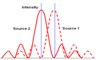
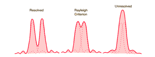
Figure 1.1: Rayleigh’s criterion and Rayleigh’s diffraction limit.

However, Rayleigh’s choice of resolution limit is based on presumed resolving ability of human visual system, which at first glance seems arbitrary. In fact, Rayleigh said about his criterion that

“This rule is convenient on account of its simplicity and it is sufficiently accurate in view of the necessary uncertainty as to what exactly is meant by resolution."

As is shown in Figure 1.1, the Rayleigh diffraction limit results in an $\sim 20\%$ dip in intensity between the two peaks of Airy disks [9]. Schuster pointed out in 1904 [37] that the dip in intensity necessary to indicate resolution is a physiological phenomenon and there are other forms of spectroscopic investigation besides that of eye observation. Many alternative criteria were proposed by other physicists as illustrated in Figure 1.2.

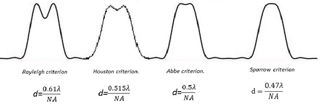
Figure 1.2: Different resolution limits.

A more mathematically rigorous criterion was proposed by Sparrow [41], who advocates that the resolution limit should be the distance between two point sources where the images no longer have a dip between the central peaks of each Airy disk (as illustrated by Figure 1.2). Based on Sparrow’s criterion, the two point sources are so close that the source locations may not be stably resolved although the source number is detected. Indeed, the Sparrow resolution limit is less relevant with practical use [6, 9] because it is very signal-to-noise dependent and has no easy comparison to a readily measured value in real images. Therefore, these classical resolution criteria focus on the smallest distance between two sources above which we can be sure that there are two sources, regardless of whether their locations can be resolved stably or not.

The classical resolution criteria mentioned above deal with calculated images that are described by a known and exact mathematical model of the intensity distribution. However, if one has perfect access to the intensity profile of the diffraction image of two point sources, one could locate the exact source despite the diffraction. There would be no resolution limit for the reconstruction. This simple fact has been noticed by many researchers in the field [12, 10, 6]. On the other hand, an imaging system constructed without any aberration or irregularity is not practical, because the shape of the point-spread function is never known exactly and the measurement noise is inevitable [35, 10]. Therefore, a rigorous and practically meaningful resolution limit could only be set when taking into account the aberrations and measurement noises [35, 16]. In this setting, the images (detected by detectors in practice) were categorized as detected images by Ronchi [35] and their resolution was advocated to be more important to investigate than the resolution defined by those classical criteria. Inspired by this, many researchers have analyzed the two-point resolution from the perspective of statistical inference [18, 19, 28, 27, 16, 38, 39, 40]. For instance, in [19] Helstrom has shown that the resolution of two identical objects depends on deciding whether they are both present in the field of view or only one of them is there, and their resolvability is measured by the probability of making this decision correctly. In all the papers mentioned above, the authors have derived quasi-explicit formulas or estimations for the minimum SNR that is required to discriminate two point sources or for the possibility of a correct decision. Although the resolutions (or the requirement) in this respect were thoroughly explored in these works which spanned the course of several decades, these results are rarely (even never) utilized in the practical applications. This is mainly because the derived resolution formulas are complicated and the results highly depend on the statistical model of the noise, which prohibits their applicability. Especially, the inevitable aberrations in the modeling will not satisfy these statistical assumptions. Overall, despite many efforts made from the 19th century to date, in practice, our understanding of when exactly two point sources can or cannot be resolved has rarely risen above heuristic arguments.

In the present paper, one of our major contributions is the theoretical and rigorous derivation of the two-point diffraction limit in imaging under only an assumption on the noise level. The diffraction limit is given by a simple and exact formula (1.2) and demonstrates that super-resolution is definitely possible when $SNR>2$. Compared to the former results on the two-point resolution, our formula is simple, effective and widely applicable due to the extremely general assumption on the noise and the imaging model.

1.1.2 Concept of super-resolution

We next introduce the concept of super-resolution. Super-resolution microscopy is a series of techniques in optical microscopy that allow such images to have resolutions higher than those imposed by the diffraction limit (Rayleigh resolution limit). Due to the breakthrough in super-resolution techniques in recent years, this topic becomes increasingly popular in various fields and the concept of super-resolution becomes very general. Some literature claims super-resolution although theoretically the sources should be separated by a distance above the Rayleigh limit. Bounds on the recovery of the amplitudes (or intensities) of the sources have been derived. Nevertheless, the original concept of super-resolution actually focuses mainly on both detecting the source number and recovering the source locations.

To the best of our knowledge, there is no unique and mathematically rigorous definition of super-resolution. On the other hand, as we have said, the number detection and location recovery are two inherently different [25] but important tasks in the super-resolution, thus we consider two different super-resolutions in the current paper. One is achieving resolution better than the Rayleigh diffraction limit in detecting the correct source number and is named "super-resolution in number detection". The other is achieving resolution better than the Rayleigh diffraction limit in stably recovering the source locations and is named "super-resolution in location recovery".

1.1.3 Previous mathematical contributions

Based on Rayleigh’s criterion, the corresponding resolution limit for imaging with the point spread function $\mathrm{sinc}(||\boldsymbol{\mathbf{x}}||_{2})^{2}$ is $\frac{\pi}{\Omega}$. On the other hand, it was shown by many mathematical studies that $\frac{\pi}{\Omega}$ is also the critical limit for the imaging model (1.1). To be more specific, in [13] Donoho demonstrated that for sources on grid points spacing by $\Delta\geq\frac{\pi}{\Omega}$, the stable recovery is possible from (1.1) in dimension one, but the stability becomes much worse in the case when $\Delta<\frac{\pi}{\Omega}$. Therefore, in the same way as [13], we regard $\frac{\pi}{\Omega}$ as the Rayleigh limit in this paper, and super-resolution refers to obtaining a better resolution than $\frac{\pi}{\Omega}$.

For the mathematical theory of super-resolving $n$ point sources or infinity point sources, to the best of our knowledge, the first result was derived by Donoho in 1992 [13]. He developed a theory from the optimal recovery point of view to explain the possibility and difficulties of super-resolution via sparsity constraint. He considered measures supported on a lattice $\{k\Delta\}_{k=-\infty}^{\infty}$ and regularized by a so-called “Rayleigh index” $R$. The available measurement is the noisy Fourier data of the discrete measure with frequency cutoff $\Omega$. He showed that the minimax error $E^{*}$ for the amplitude recovery with noise level $\sigma$ was bounded as

$$\beta_{1}(R,\Omega)\left(\frac{1}{\Delta}\right)^{2R-1}\sigma\leq E^{*}\leq\beta_{2}(R,\Omega)\left(\frac{1}{\Delta}\right)^{4R+1}\sigma$$

for certain small $\Delta$. His results emphasize the importance of sparsity in the super-resolution. In recent years, due to the impressive development of super-resolution modalities in biological imaging [17, 46, 20, 4, 36] and super-resolution algorithms in applied mathematics [5, 14, 32, 44, 43, 31, 30, 11], the inherent super-resolving capacity of the imaging problem becomes increasingly popular and the one-dimensional case was well-studied. In [8], the authors considered resolving the amplitudes of $n$-sparse point sources supported on a grid and improved the results of Donoho. Concretely, they showed that the scaling of the noise level for the minimax error should be $SRF^{2n-1}$, where $SRF:=\frac{1}{\Delta\Omega}$ is the super-resolution factor. Similar results for multi-clumps cases were also derived in [2, 21]. Recently in [3], the authors derived sharp minimax errors for the location and the amplitude recovery of off-the-grid sources. They showed that for $\sigma\lesssim(SRF)^{-2p+1}$, where $p$ is the number of nodes that form a cluster of certain type, the minimax error rate for reconstruction of the clustered nodes is of the order $(SRF)^{2p-2}\frac{\sigma}{\Omega}$, while for recovering the corresponding amplitudes the rate is of the order $(SRF)^{2p-1}\sigma$. Moreover, the corresponding minimax rates for the recovery of the non-clustered nodes and amplitudes are $\frac{\sigma}{\Omega}$ and $\sigma$ respectively. We also refer the readers to [29, 6] for understanding the resolution limit from the perceptive of sample complexity and to [42, 7] for the resolving limit of some algorithms.

On the other hand, in order to characterize the exact resolution rather than the minimax error in recovering multiple point sources, in the earlier works [26, 25, 24, 22] we have defined the so-called "computational resolution limits", which characterize the minimum required distance between point sources so that their number and locations can be stably resolved under certain noise level. By developing a nonlinear approximation theory in so-called Vandermonde spaces, we have derived sharp bounds for computational resolution limits in the one-dimensional super-resolution problem. In particular, we have showed in [25] that the computational resolution limits for the number and location recoveries should be bounded above by respectively $\frac{4.4e\pi}{\Omega}\left(\frac{\sigma}{m_{\min}}\right)^{\frac{1}{2n-2}}$ and $\frac{5.88e\pi}{\Omega}\left(\frac{\sigma}{m_{\min}}\right)^{\frac{1}{2n-1}}$. By these works, we raise our understanding of the stability of the super-resolution above only heuristic arguments. In the present paper, we substantially improve these estimates to have practical significance.

1.2 Our main contributions in this paper

This paper is devoted to elucidating the essence of super-resolution and deals mainly with the stability of super-resolution and the diffraction limit. We consider the imaging problem as recovering the sources $\mu=\sum_{j=1}^{n}a_{j}\delta_{\boldsymbol{\mathbf{y}}_{j}},\boldsymbol{\mathbf{y}}_{j}\in\mathbb{R}^{k}$ from its noisy Fourier data,

$$\mathbf{Y}(\boldsymbol{\mathbf{\omega}})=\mathcal{F}[\mu](\boldsymbol{\mathbf{\omega}})+\mathbf{W}(\boldsymbol{\mathbf{\omega}})=\sum_{j=1}^{n}a_{j}e^{i\boldsymbol{\mathbf{y}}_{j}\cdot\boldsymbol{\mathbf{\omega}}}+\mathbf{W}(\boldsymbol{\mathbf{\omega}}),\ \boldsymbol{\mathbf{\omega}}\in\mathbb{R}^{k},\ ||\boldsymbol{\mathbf{\omega}}||_{2}\leq\Omega,$$ (1.1)

where $\boldsymbol{\mathbf{W}}$ represents the total effect of noise and aberrations. This is a common model in mathematics for theoretically analyzing the imaging problem [13, 5, 3]. It is directly the model in the frequency domain for the imaging modalities with $\mathrm{sinc}(||\boldsymbol{\mathbf{x}}||_{2})$ being the point spread function [10]. Its discrete form is also a standard model called line spectral estimation in the fields of array processing, signal processing, and wireless communications. On the other hand, even for imaging with general point spread functions or optical transfer functions, some of the imaging enhancements such as inverse filtering method [15] will modify the measurements in the frequency domain to (1.1). This ensures that our model has sufficient practical background and significance and that our results can be applied to a wide range of imaging systems.

From model (1.1) in dimension one, our first contribution is two location-amplitude-identities characterizing the relations between source locations and amplitudes in the one-dimensional super-resolution problem. These identities allow us to directly derive the super-resolution capability for number, location, and amplitude recovery in the super-resolution problem and improve state-of-the-art estimations to an unprecedented level to have practical significance. Although these nonlinear inverse problems are known to be very challenging, we now have a clear and simple picture of all of them, which allows us to solve them in a unified way in just a few pages. To be more specific, we prove that it is definitely possible to detect the correct source number when the sources are separated by

$$\min_{p\neq j}\Big{|}y_{p}-y_{j}\Big{|}\geq\frac{2e\pi}{\Omega}\Big{(}\frac{\sigma}{m_{\min}}\Big{)}^{\frac{1}{2n-2}},$$

where $y_{j}$’s are one-dimensional source locations and $\frac{\sigma}{m_{\min}}$ represents the inverse of the signal-to-noise ratio ($SNR$). This substantially improves the estimate in [25] and indicates that super-resolution in detecting correct source number (i.e., surpassing the diffraction limit $\frac{\pi}{\Omega}$) is definitely possible when $\frac{m_{\min}}{\sigma}\geq(2e)^{2n-2}$. Moreover, for the case when resolving two sources, the requirement for the separation is improved to

$$\min_{p\neq j}\Bigg{|}y_{p}-y_{j}\Bigg{|}\geq\frac{2\arcsin\left(2\left(\frac{\sigma}{m_{\min}}\right)^{\frac{1}{2}}\right)}{\Omega},$$

indicating that surpassing the Rayleigh limit in distinguishing two sources is definitely possible when $SNR>4$. This is the first time where it is demonstrated theoretically that super-resolution (’in number detection’) is actually possible. For the stable location recovery, the estimate is improved to

$$\min_{p\neq j}\left|y_{p}-y_{j}\right|\geq\frac{2.36e\pi}{\Omega}\Big{(}\frac{\sigma}{m_{\min}}\Big{)}^{\frac{1}{2n-1}}$$

as compared to the previous result in [25], indicating that the location recovery is stable when $\frac{m_{\min}}{\sigma}\geq(2.36e)^{2n-1}$. These results provide us with quantitative understandings of the super-resolution of multiple sources. Moreover, since our method is rather direct, it is very hard to substantially improve the estimates now and we even roughly know to what extent the constant factor in the estimates can be improved.

Our second crucial result is the theoretical proof of a two-point diffraction limit in spaces of general dimensionality under only an assumption on the noise level. It is given by

$$\mathcal{R}=\frac{4\arcsin\left(\left(\frac{\sigma}{m_{\min}}\right)^{\frac{1}{2}}\right)}{\Omega}$$ (1.2)

for $\frac{\sigma}{m_{\min}}\leq\frac{1}{2}$. In the case when $\frac{\sigma}{m_{\min}}>\frac{1}{2}$, there is no super-resolution under certain circumstances. This solves the long-standing puzzle and debate about the diffraction limit for imaging in general setting. We also generalize the results to the case when resolving two arbitrary sources. Our results show that, for the resolution of any two point sources, when $SNR>2$, one can definitely exceed the Rayleigh limit. When $SNR>4$, one can already achieve $1.5$ times improvement of the Rayleigh limit. This finding indicates that obtaining resolution far better than the Rayleigh limit is actually possible by refined sensors.

Our results can be directly extended to the following more general setting:

$$\mathbf{Y}(\boldsymbol{\mathbf{\omega}})=\chi(\boldsymbol{\mathbf{\omega}})\mathcal{F}[\mu](\boldsymbol{\mathbf{\omega}})+\mathbf{W}(\boldsymbol{\mathbf{\omega}})=\sum_{j=1}^{n}a_{j}\chi(\boldsymbol{\mathbf{\omega}})e^{i\boldsymbol{\mathbf{y}}_{j}\cdot\boldsymbol{\mathbf{\omega}}}+\mathbf{W}(\boldsymbol{\mathbf{\omega}}),\ \boldsymbol{\mathbf{\omega}}\in\mathbb{R}^{k},\ ||\boldsymbol{\mathbf{\omega}}||_{2}\leq\Omega,$$ (1.3)

where $\chi(\boldsymbol{\mathbf{\omega}})=0$ or $1$, $\chi(\boldsymbol{\mathbf{0}})=1$ and $\chi(\boldsymbol{\mathbf{\omega}})=1,||\boldsymbol{\mathbf{\omega}}||_{2}=\Omega$. This enables the application of our results to imaging from discretely sampled data and line spectral estimations in array processing. Moreover, our findings can be applied to imaging systems with general optical transfer functions. A new fact revealed in this paper is that the two-point resolution is actually determined by the boundary points of the transfer function and is not that dependent to the interior frequency information. Also, as revealed in Section 3.1, the measurements at $\boldsymbol{\mathbf{\omega}}=\boldsymbol{\mathbf{0}}$ and $\left|\left|{\boldsymbol{\mathbf{\omega}}}\right|\right|=\Omega$ are already enough for the algorithm which provably achieves the resolution limit.

In the last part of the paper, we find an algorithm that achieves the optimal resolution when distinguishing two sources and conduct many numerical experiments to manifest its optimal performance and phase transition. Although the noise and the aberration is inevitable and the point source is not an exact delta point, our results still indicate that super-resolving two sources in practice is possible for general imaging modalities, due to the proved excellent noise tolerance. We plan to examine the practical feasibility of our method in a near future.

To summarize, by this paper we have shed lights on understanding quantitatively when super-resolution is definitely possible and when is not. It has been disclosed by our results that super-resolution when distinguishing two sources is far more possible than what was commonly recognized. By this work, we hope to inspire a start of a new period where examining the resolution based on the signal-to-noise ratio becomes a feasible method in the field of imaging, which is also the hope of many physicists and opticists [35].

1.3 Organization of the paper

The paper is organized in the following way. In Section 2, we present the theory of location-amplitude identities. In Section 3, we derive stability results for recovering the number, locations, and amplitudes of sources in the one-dimensional super-resolution problem. In Section 4, we derive the exact formula of the two-point resolution limit and, in Section 5, we devise algorithms achieving exactly the optimal resolution in distinguishing images from one and two sources. The Appendix consists of some useful inequalities.

2 Location-amplitude identities

In this section, we intend to derive two location-amplitude identities that characterize the relations between source locations and amplitudes in the super-resolution problem. We start from the following elementary model:

$$\mathcal{F}[\hat{\mu}](\omega)=\mathcal{F}[\mu](\omega)+\boldsymbol{\mathbf{w}}(\omega),\quad\omega\in[0,\Omega],$$ (2.1)

where $\hat{\mu},\mu$ are discrete measures, $\mathcal{F}[f]=\int_{\mathbb{R}}e^{iy\omega}f(y)dy$ denotes the Fourier transform, $\boldsymbol{\mathbf{w}}$ represents the noise or the aberration, and $\Omega$ is the cutoff frequency of the imaging system. To be more specific, we set $\mu=\sum_{j=1}^{n}a_{j}\delta_{y_{j}}$ and $\hat{\mu}=\sum_{j=1}^{k}\hat{a}_{j}\delta_{\hat{y}_{j}}$ with $a_{j},\hat{a}_{j}$ being the source amplitudes and $y_{j},\hat{y}_{j}$ the source locations.

2.1 Statement of the identities

Based on the above model, we have the following location-amplitude identities.

Theorem 2.1.

[Location-amplitude identities] Consider the model

$$\mathcal{F}[\hat{\mu}](\omega)=\mathcal{F}[\mu](\omega)+\boldsymbol{\mathbf{w}}(\omega),\quad\omega\in[0,\Omega],$$

where $\hat{\mu}=\sum_{j=1}^{k}\hat{a}_{j}\delta_{\hat{y}_{j}}$ with distinct $\hat{y}_{j}$’s and $\mu=\sum_{j=1}^{n}a_{j}\delta_{y_{j}}$ with distinct $y_{j}$’s. For any $y_{j}$, let $\hat{y}_{j^{\prime}}$ be the one in the set of the $\hat{y}_{j}$’s that is the closest to $y_{j}$. Denote by $S$ the set containing exactly $y_{p},1\leq p\leq n,p\neq j,$ and those $\hat{y}_{l},l\neq j^{\prime},l=1,\cdots,k,$ that are not equal to any $y_{p}$. Then for any $0<\omega^{*}\leq\frac{\Omega}{\#S}$ such that $e^{iy_{j}\omega^{*}},e^{iq\omega^{*}},q\in S$ are still pairwise distinct, we have the following relations:

$$\hat{a}_{j^{\prime}}\Pi_{q\in S}\frac{e^{i\hat{y}_{j^{\prime}}\omega^{*}}-e^{iq\omega^{*}}}{e^{iy_{j}\omega^{*}}-e^{iq\omega^{*}}}=a_{j}+\frac{\boldsymbol{\mathbf{w}}_{1}^{\top}\boldsymbol{\mathbf{v}}}{\Pi_{q\in S}(e^{iy_{j}\omega^{*}}-e^{iq\omega^{*}})}.$$ (2.2)

Moreover, for any $0<\omega^{*}\leq\frac{\Omega}{\#S+1}$ such that $e^{iy_{j}\omega^{*}},e^{iq\omega^{*}},q\in S$ are still pairwise distinct, we have

$$(e^{i\hat{y}_{j^{\prime}}\omega^{*}}-e^{iy_{j}\omega^{*}})a_{j}=\frac{\left(e^{i\hat{y}_{j^{\prime}}\omega^{*}}\boldsymbol{\mathbf{w}}_{1}-\boldsymbol{\mathbf{w}}_{2}\right)^{\top}\boldsymbol{\mathbf{v}}}{\Pi_{q\in S}(e^{iy_{j}\omega^{*}}-e^{iq\omega^{*}})}.$$ (2.3)

Here, $\boldsymbol{\mathbf{w}}_{1}=(\boldsymbol{\mathbf{w}}(0),\boldsymbol{\mathbf{w}}(\omega^{*}),\cdots,\boldsymbol{\mathbf{w}}((\#s)\omega^{*}))^{\top}$, $\boldsymbol{\mathbf{w}}_{2}=(\boldsymbol{\mathbf{w}}(1),\boldsymbol{\mathbf{w}}(\omega^{*}),\cdots,\boldsymbol{\mathbf{w}}((\#s+1)\omega^{*}))^{\top}$ and the vector $\boldsymbol{\mathbf{v}}$ is given by

$$\left((-1)^{\#S}\sum_{(q_{1},\cdots,q_{\#S})\in S_{\#S}}e^{iq_{1}\omega^{*}}\cdots e^{iq_{\#S}\omega^{*}},(-1)^{\#S-1}\sum_{(q_{1},\cdots,q_{\#S-1})\in S_{\#S-1}}e^{iq_{1}\omega^{*}}\cdots e^{iq_{\#S-1}\omega^{*}},\cdots,(-1)\sum_{(q_{1})\in S_{1}}e^{iq_{1}\omega^{*}},1\right)^{\top},$$

where $S_{j}:=\left\{(q_{1},\cdots,q_{j})\bigg{|}q_{t}\in S,1\leq t\leq j,q_{t}\neq q_{t^{\prime}}\text{ for }t\neq t^{\prime}\right\}$, $\ j=1,\cdots,\#S$.

Theorem 2.1 reveals in depth the essence of the super-resolution problem. From (2.2), we observe that

$$\hat{a}_{j^{\prime}}g-a_{j}=\frac{\boldsymbol{\mathbf{w}}_{1}^{\top}\boldsymbol{\mathbf{v}}}{\Pi_{q\in S}(e^{iy_{j}\omega^{*}}-e^{iq\omega^{*}})}$$ (2.4)

for a certain $g$ that is close to $1$ when $\hat{y}_{j^{\prime}}$ and $y_{j}$ are close to each other. This shows the relation between the amplitudes of the underlying sources and the recovered sources. Note that the quantity $\boldsymbol{\mathbf{w}}_{1}^{T}\boldsymbol{\mathbf{v}}$ in the RHS of (2.4) is from the noise or the aberration and is of order of the noise level. Thus the stability of the amplitude recovery is obviously determined by $\frac{1}{\Pi_{q\in S}(e^{iy_{j}\omega^{*}}-e^{iq\omega^{*}})}$, which is further determined by the distribution of the locations of the underlying sources and the recovered ones. As there are around $2n-2$ sources in $S$ for a stable recovery, the noise amplification factor is thus around $\left(\frac{1}{d_{\min}}\right)^{2n-2}$ with $d_{\min}$ being the minimum separation distance between the sources. This is why the factors $\left(\frac{1}{d_{\min}}\right)^{2n-2},\left(\frac{1}{d_{\min}}\right)^{2n-1}$ frequently appear in the stability analysis of the amplitude and the location (by (2.3)) recoveries [3, 25] even when the problem is explored by methods different from those introduced here. Transforming the stability of the amplitude recovery into a simpler problem of analyzing $\frac{1}{\Pi_{q\in S}(e^{iy_{j}\omega^{*}}-e^{iq\omega^{*}})}$ under certain conditions, enables us to derive a stability result for the amplitude recovery in Section 3.3 in a rather straightforward manner.

On the other hand, identity (2.3) reveals directly the relation between the locations of the underlying sources and the recovered ones. It is rather obvious now that the stability of location recovery is exactly determined by $\frac{\sigma}{\Pi_{q\in S}(e^{iy_{j}\omega^{*}}-e^{iq\omega^{*}})}$ with $\sigma$ representing the noise level. By this understanding, we prove in Sections 3.1 and 3.2 respectively the stability of the number detection and location recovery in the super-resolution problem.

For the convenience of the applications of our location-amplitude identities, we derive the following corollary, as a direct consequence of Theorem 2.1.

Corollary 2.1.

Consider the model

$$\mathcal{F}[\hat{\mu}](\omega)=\mathcal{F}[\mu](\omega)+\boldsymbol{\mathbf{w}}(\omega),\quad\omega\in[0,\Omega],$$

where $\hat{\mu}=\sum_{j=1}^{k}\hat{a}_{j}\delta_{\hat{y}_{j}}$ with distinct $\hat{y}_{j}$’s and $\mu=\sum_{j=1}^{n}a_{j}\delta_{y_{j}}$ with distinct $y_{j}$’s and assume that $|\boldsymbol{\mathbf{w}}(\omega)|<\sigma,\omega\in[0,\Omega]$. For any $y_{j}$, let $\hat{y}_{j^{\prime}}$ be the one in the set of the $\hat{y}_{j}$’s that is the closest to $y_{j}$. Denote by $S$ the set containing exactly $y_{p},1\leq p\leq n,p\neq j,$ and those $\hat{y}_{l},l\neq j^{\prime},l=1,\cdots,k,$ that are not equal to any $y_{p}$. Then for any $0<\omega^{*}\leq\frac{\Omega}{\#S}$ such that $e^{iy_{j}\omega^{*}},e^{iq\omega^{*}},q\in S$ are still pairwise distinct, we have

$$\left|\hat{a}_{j^{\prime}}\Pi_{q\in S}\frac{e^{i\hat{y}_{j^{\prime}}\omega^{*}}-e^{iq\omega^{*}}}{e^{iy_{j}\omega^{*}}-e^{iq\omega^{*}}}-a_{j}\right|<\frac{2^{\#S}\sigma}{\Pi_{q\in S}\left|e^{iy_{j}\omega^{*}}-e^{iq\omega^{*}}\right|}.$$ (2.5)

Moreover, for any $0<\omega^{*}\leq\frac{\Omega}{\#S+1}$ such that $e^{iy_{j}\omega^{*}},e^{iq\omega^{*}},q\in S$ are still pairwise distinct,

$$\left|(e^{i\hat{y}_{j^{\prime}}\omega^{*}}-e^{iy_{j}\omega^{*}})a_{j}\right|<\frac{2^{\#S+1}\sigma}{\Pi_{q\in S}\left|e^{iy_{j}\omega^{*}}-e^{iq\omega^{*}}\right|}.$$ (2.6)

Proof.

This is a direct consequence of Theorem 2.1 in view of

$$|\boldsymbol{\mathbf{w}}_{1}^{\top}\boldsymbol{\mathbf{v}}|\leq 2^{\#S}\sigma,\qquad|(e^{i\hat{y}_{j^{\prime}}\omega^{*}}\boldsymbol{\mathbf{w}}_{1}-\boldsymbol{\mathbf{w}}_{2})^{\top}\boldsymbol{\mathbf{v}}|\leq 2^{\#S+1}\sigma.$$

∎

2.2 Proof of Theorem 2.1

Proof.

Before starting the proof, we first introduce some notation and lemmas. Denote by

$$\phi_{p,q}(t)=\left(t^{p},t^{p+1},\cdots,t^{q}\right)^{\top}.$$ (2.7)

The following lemma on the inverse of the Vandermonde matrix is standard.

Lemma 2.2.

Let $V_{k}$ be the Vandermonde matrix $\left(\phi_{0,k-1}(t_{1}),\cdots,\phi_{0,k-1}(t_{k})\right)$. Then its inverse $V_{k}^{-1}=B$ can be specified as follows:

$$B_{jq}=\left\{\begin{array}[]{cc}(-1)^{k-q}\left(\frac{\sum_{\begin{subarray}{c}1\leq m_{1}<\ldots<m_{k-q}\leq k\\ m_{1},\ldots,m_{k-q}\neq j\end{subarray}}t_{m_{1}}\cdots t_{m_{k-q}}}{\prod_{\begin{subarray}{c}1\leq m\leq k\\ m\neq j\end{subarray}}\left(t_{j}-t_{m}\right)}\right),&\quad 1\leq q<k,\\ \frac{1}{\prod_{\begin{subarray}{c}1\leq m\leq k\\ m\neq j\end{subarray}}\left(t_{j}-t_{m}\right)},&\quad q=k.\end{array}\right.$$

The following lemma can be deduced from the inverse of the Vandermonde matrix and the readers can check Lemma 5 in [25] for a simple proof, although the numbers there are real numbers.

Lemma 2.3.

Let $t_{1},\cdots,t_{k},$ be $k$ different complex numbers. For $t\in\mathbb{C}$, we have

$$\left(V_{k}^{-1}\phi_{0,k-1}(t)\right)_{j}=\Pi_{1\leq q\leq k,q\neq j}\frac{t-t_{q}}{t_{j}-t_{q}},$$

where $V_{k}:=\big{(}\phi_{0,k-1}(t_{1}),\cdots,\phi_{0,k-1}(t_{k})\big{)}$ with $\phi_{0,k-1}(\cdot)$ being defined by (2.7).

Now we start the main proof. We only prove the theorem for $\omega^{*}\leq\frac{\Omega}{\#S+1}$. The case when $\omega^{*}\leq\frac{\Omega}{\#S}$ for (2.2) is obvious afterwards. From (2.1), we can write

$$\hat{A}\hat{a}=Aa+W$$ (2.8)

where $\hat{a}=(\hat{a}_{1},\cdots,\hat{a}_{k})^{\top}$, $a=(a_{1},\cdots,a_{n})^{\top},W=(\boldsymbol{\mathbf{w}}(0),\cdots,\boldsymbol{\mathbf{w}}(\#S+1))^{\top}$ and

$$\hat{A}=\left(\phi_{0,\#S+1}(e^{i\hat{y}_{1}\omega^{*}}),\ \phi_{0,\#S+1}(e^{i\hat{y}_{2}\omega^{*}}),\ \cdots,\ \phi_{0,\#S+1}(e^{i\hat{y}_{k}\omega^{*}})\right),$$

$$A=\left(\phi_{0,\#S+1}(e^{iy_{1}\omega^{*}}),\ \phi_{0,\#S+1}(e^{iy_{2}\omega^{*}}),\ \cdots,\ \phi_{0,\#S+1}(e^{iy_{n}\omega^{*}})\right),$$

with $0<\omega^{*}\leq\frac{\Omega}{\#S+1}$. We further decompose (2.8) into the following two equations:

$$\hat{a}_{j^{\prime}}\phi_{0,\#S}(e^{i\hat{y}_{j^{\prime}}\omega^{*}})=B_{1}b+\boldsymbol{\mathbf{w}}_{1},\quad\hat{a}_{j^{\prime}}\phi_{1,\#S+1}(e^{i\hat{y}_{j^{\prime}}\omega^{*}})=B_{2}b+\boldsymbol{\mathbf{w}}_{2}$$ (2.9)

where $\boldsymbol{\mathbf{w}}_{1}=(\boldsymbol{\mathbf{w}}(0),\cdots,\boldsymbol{\mathbf{w}}(\#S))^{\top}$, $\boldsymbol{\mathbf{w}}_{2}=(\boldsymbol{\mathbf{w}}(1),\cdots,\boldsymbol{\mathbf{w}}(\#S+1))^{\top}$ and

$$B_{1} =\left(\phi_{0,\#S}(e^{iy_{1}\omega^{*}}),\cdots,\phi_{0,\#S}(e^{iy_{n}\omega^{*}}),\phi_{0,\#S}(e^{i\hat{y}_{j_{1}}\omega^{*}}),\cdots,\phi_{0,\#S}(e^{i\hat{y}_{j_{\#S+1-n}}\omega^{*}})\right),$$

$$B_{2} =\left(\phi_{1,\#S+1}(e^{iy_{1}\omega^{*}}),\cdots,\phi_{1,\#S+1}(e^{iy_{n}\omega^{*}}),\phi_{1,\#S+1}(e^{i\hat{y}_{j_{1}}\omega^{*}}),\cdots,\phi_{1,\#S+1}(e^{i\hat{y}_{j_{\#S+1-n}}\omega^{*}})\right)$$

with the $\hat{y}_{j_{q}}$’s being contained in $S$. Thus the $b=(b_{1},\cdots,b_{\#S+1})$ in (2.9) should be

$$b_{l}=\left\{\begin{array}[]{ll}a_{j},&l=j,\\ a_{l}-\hat{a}_{q_{l}},&1\leq l\leq n,l\neq j,\text{and $y_{l}=\hat{y}_{q_{l}}$ for certain $q_{l}$},\\ a_{l},&1\leq l\leq n,l\neq j,\text{and $y_{l}\neq\hat{y}_{q},q=1,\cdots,k$},\\ \hat{a}_{j_{l-n}},&l>n.\end{array}\right.$$

Note that the fact that $b_{l}=a_{j},l=j$ is because $\hat{y}_{j^{\prime}}$ is the point in $\hat{y}_{q}$’s that is the closest to $y_{j}$, there is no other $\hat{y}_{q}$ equals to $y_{j}$. Observe that

$$B_{2}=B_{1}\mathrm{diag}\left(e^{iy_{1}\omega^{*}},\cdots,e^{iy_{n}\omega^{*}},e^{i\hat{y}_{j_{1}}\omega^{*}},\cdots,e^{i\hat{y}_{j_{\#S+1-n}}\omega^{*}}\right),\ \phi_{1,\#S+1}(e^{iy_{l}\omega^{*}})=e^{iy_{l}\omega^{*}}\phi_{0,\#S}(e^{iy_{l}\omega^{*}}),$$

we rewrite (2.9) as

$$\hat{a}_{j^{\prime}}\phi_{0,\#S}(e^{i\hat{y}_{j^{\prime}}\omega^{*}})=B_{1}b+W_{1},$$ (2.10)

$$e^{i\hat{y}_{j^{\prime}}\omega^{*}}\hat{a}_{j^{\prime}}\phi_{0,\#S}(e^{i\hat{y}_{j^{\prime}}\omega^{*}})=B_{1}\mathrm{diag}\left(e^{iy_{1}\omega^{*}},\cdots,e^{iy_{n}\omega^{*}},e^{i\hat{y}_{j_{1}}\omega^{*}},\cdots,e^{i\hat{y}_{j_{\#S+1-n}}\omega^{*}}\right)b+W_{2}.$$

Since $e^{iy_{j}\omega^{*}}$ and all the points $e^{iq\omega^{*}}$ for $q$ in $S$ are pairwise distinct according to the setting of the theorem, $B_{1}$ is a regular matrix. We multiply both sides of the above equations by the inverse of $B_{1}$ to get from Lemma 2.3 that

$$\hat{a}_{j^{\prime}}\Pi_{q\in S}\frac{e^{i\hat{y}_{j^{\prime}}\omega^{*}}-e^{iq\omega^{*}}}{e^{iy_{j}\omega^{*}}-e^{iq\omega^{*}}} =a_{j}+(B_{1}^{-1})_{j}\boldsymbol{\mathbf{w}}_{1},$$ (2.11)

$$e^{i\hat{y}_{j^{\prime}}\omega^{*}}\hat{a}_{j^{\prime}}\Pi_{q\in S}\frac{e^{i\hat{y}_{j^{\prime}}\omega^{*}}-e^{iq\omega^{*}}}{e^{iy_{j}\omega^{*}}-e^{iq\omega^{*}}} =e^{iy_{j}\omega^{*}}a_{j}+(B_{1}^{-1})_{j}\boldsymbol{\mathbf{w}}_{2},$$ (2.12)

where $(B_{1}^{-1})_{j}$ is the $j$-th row of $B_{1}^{-1}$. By Lemma 2.2, it follows that

$$(B_{1}^{-1})_{j}W_{1}=\frac{\sum_{p=0}^{\#S-1}\left(\boldsymbol{\mathbf{w}}(p)(-1)^{\#S-p}\sum_{(q_{1},\cdots,q_{\#S-p})\in S_{\#S-p}}e^{iq_{1}\omega^{*}}\cdots e^{iq_{\#S-p}\omega^{*}}\right)+\boldsymbol{\mathbf{w}}(\#s)}{\Pi_{q\in S}(y_{j}-q)}.$$ (2.13)

This proves (2.2). Furthermore, equation (2.11) times $e^{i\hat{y}_{j^{\prime}}\omega^{*}}$ minus (2.12) yields

$$(e^{i\hat{y}_{j^{\prime}}\omega^{*}}-e^{iy_{j}\omega^{*}})a_{j}=(B_{1}^{-1})_{j}\left(e^{i\hat{y}_{j^{\prime}}\omega^{*}}\boldsymbol{\mathbf{w}}_{1}-\boldsymbol{\mathbf{w}}_{2}\right).$$

Similarly, further expanding $(B_{1}^{-1})_{j}\left(e^{i\hat{y}_{j^{\prime}}\omega^{*}}\boldsymbol{\mathbf{w}}_{1}-\boldsymbol{\mathbf{w}}_{2}\right)$ explicitly by Lemma 2.2 yields (2.3). This completes the proof. ∎

3 Stability of super-resolution

In this section, based on our location-amplitude identities, we analyze the super-resolution capability of the reconstruction of the numbers, locations, and amplitudes of the off-grid sources in the super-resolution problem. Note that these problems have been analyzed in [25, 3] from different perspectives but the proofs are over several tens of pages. Now, by our method, we have a direct and clear picture of all these problems, which allows us to prove them in a unified way and in less than ten pages. In particular, this new method improves the estimation of computational resolution bounds in our previous work [25] to an unprecedented level to have practical meanings. This is also the ultimate goal of our definition of computational resolution limits.

We consider only the one-dimensional super-resolution problem since the generalization to multi-dimensions is straightforward by the method in [24]. Let us introduce the model setting. We consider the collection of point sources as a discrete measure $\mu=\sum_{j=1}^{n}a_{j}\delta_{y_{j}}$, where $y_{j}\in\mathbb{R},j=1,\cdots,n$, represent the location of the point sources and the $a_{j}$’s their amplitudes. Noting that the $y_{j}$’s are the supports of the Dirac masses in $\mu$. Throughout the paper, we will use the supports recovery for a substitution of the location reconstruction.

We denote by

$$m_{\min}=\min_{j=1,\cdots,n}|a_{j}|,\quad d_{\min}=\min_{p\neq j}|y_{p}-y_{j}|.$$ (3.1)

The measurement is the noisy Fourier data of $\mu$ in a bounded interval, that is,

$$\mathbf{Y}(\omega)=\mathcal{F}[\mu](\omega)+\mathbf{W}(\omega)=\sum_{j=1}^{n}a_{j}e^{iy_{j}\omega}+\mathbf{W}(\omega),\quad\omega\in[-\Omega,\Omega],$$ (3.2)

with $\mathbf{W}(\omega)$ being the noise and $\Omega$ the cutoff frequency of the imaging system. We assume that

$$|\mathbf{W}(\omega)|<\sigma,\qquad\omega\in[-\Omega,\Omega],$$

with $\sigma$ being the noise level. Note that although we consider the absolute bound here, our estimates can be extended to other kinds of bounds of the noise.

Since we focus on the resolution limit case, we consider the case when the point sources are tightly spaced and form a cluster. To be more specific, we define the interval

$$I(n,\Omega):=\Big{(}-\frac{(n-1)\pi}{2\Omega},\quad\frac{(n-1)\pi}{2\Omega}\Big{)},$$

which is of the length of several Rayleigh limits and assume that $y_{j}\in I(n,\Omega),1\leq j\leq n$. This assumption is a common assumption for super-resolving the off-the-grid sources [25, 3] and is necessary for the analysis. Since we are interested in resolving closely-spaced sources, it is also reasonable.

The reconstruction process is usually targeting at some specific solutions in a so-called admissible set, which comprises discrete measures whose Fourier data are sufficiently close to $\boldsymbol{\mathbf{Y}}$. In general, every admissible measure is possibly the ground truth and it is impossible to distinguish which one is closer to the ground truth without any additional prior information. In our problem, we introduce the following concept of $\sigma$-admissible discrete measures. For simplicity, we also call them $\sigma$-admissible measures.

Definition 3.1.

Given the measurement $\mathbf{Y}$, $\hat{\mu}=\sum_{j=1}^{k}\hat{a}_{j}\delta_{\hat{y}_{j}}$ is said to be a $\sigma$-admissible discrete measure of   $\mathbf{Y}$ if

$$\left|{\mathcal{F}[\hat{\mu}](\omega)-\mathbf{Y}(\omega)}\right|<\sigma,\quad\omega\in[-\Omega,\Omega].$$

3.1 Stability of number detection

In this section, we estimate the super-resolving capability of number detection in the super-resolution problem. We introduce the concept of computational resolution limit for number detection [26, 25, 24] and present a sharp bound for it. We improve the estimate substantially and make it have some practical meaning.

Note the set of $\sigma$-admissible measures of $\mathbf{Y}$ characterizes all possible solutions to our super-resolution problem with the given measurement $\mathbf{Y}$. Detecting the source number $n$ is possible only if all of the admissible measures have at least $n$ supports, otherwise, it is impossible to detect the correct source number without additional a prior information. Thus, following definitions similar to those in [25, 26, 24], we define the computational resolution limit for the number detection problem as follows.

Definition 3.2.

The computational resolution limit to the number detection problem in the super-resolution of one-dimensional source is defined as the smallest nonnegative number $\mathcal{D}_{num}$ such that for all $n$-sparse measure $\sum_{j=1}^{n}a_{j}\delta_{y_{j}},y_{j}\in I(n,\Omega)$ and the associated measurement $\boldsymbol{\mathbf{Y}}$ in (3.2), if

$$\min_{p\neq j}|y_{j}-y_{p}|\geq\mathcal{D}_{num},$$

then there does not exist any $\sigma$-admissible measure of   $\mathbf{Y}$ with less than $n$ supports.

The definition of “computational resolution limit” emphasizes the essential impossibility of correctly detecting the number of very close sources by any means, in contrast to the Rayleigh limit, which only concerns the visual capacity of human eyes. Moreover, it depends crucially on the signal-to-noise ratio and the sparsity of the sources, which is fundamentally different from all the classical resolution limits [1, 45, 34, 37, 41] that depend only on the cutoff frequency. We now present a sharp upper bound for it.

Theorem 3.1.

Let $\mathbf{Y}$ be a measurement generated by a measure $\mu=\sum_{j=1}^{n}a_{j}\delta_{y_{j}}$ which is supported on $I(n,\Omega)$. Let $n\geq 2$ and assume that the following separation condition is satisfied

$$\min_{p\neq j}\Big{|}y_{p}-y_{j}\Big{|}\geq\frac{2e\pi}{\Omega}\Big{(}\frac{\sigma}{m_{\min}}\Big{)}^{\frac{1}{2n-2}},$$ (3.3)

where $m_{\min}$ is defined in (3.1). Then there does not exist any $\sigma$-admissible measures of  $\mathbf{Y}$ with less than $n$ supports. Moreover, for the cases when $n=2$ and $n=3$, if

$$\min_{p\neq j}\Bigg{|}y_{p}-y_{j}\Bigg{|}\geq\frac{2\arcsin\left(2\left(\frac{\sigma}{m_{\min}}\right)^{\frac{1}{2}}\right)}{\Omega},\quad\min_{p\neq j}\Bigg{|}y_{p}-y_{j}\Bigg{|}\geq\frac{2\pi}{\Omega}\Big{(}\frac{8\sigma}{m_{\min}}\Big{)}^{\frac{1}{4}},\quad\text{respectively},$$

then there does not exist any $\sigma$-admissible measures of  $\mathbf{Y}$ with only $n-1$ supports.

Theorem 3.1 gives a better upper bound for the computational resolution limit $\mathcal{D}_{num}$ compared to the one in [25]. By the new estimate (3.1), it is already possible to surpass the Rayleigh limit $\frac{\pi}{\Omega}$ in detecting source number when $\frac{m_{\min}}{\sigma}\geq(2e)^{2n-2}$. Moreover, this upper bound is shown to be sharp by a lower bound provided in [23]. Thus, we can conclude that

$$\frac{2e^{-1}}{\Omega}\Big{(}\frac{\sigma}{m_{\min}}\Big{)}^{\frac{1}{2n-2}}<\mathcal{D}_{num}\leq\frac{2e\pi}{\Omega}\Big{(}\frac{\sigma}{m_{\min}}\Big{)}^{\frac{1}{2n-2}}.$$

In particular, for the case when $n=2$, our estimate demonstrates that when the signal-to-noise ratio $SNR>4$, then the resolution is definitely better than the Rayleigh limit and the "super-resolution in number detection" can be exactly achieved thusly. This result is already practically important. As we will see later, our estimate is very sharp and very close to the true diffraction limit.

Remark 3.1.

Note that the resolution estimate in Theorem 3.1 for the case when $n=2$ holds in general dimensional spaces. We will discuss the extension in Section 4 and give an exact two-point resolution there. It is also easy to generalize the estimates in Theorem 3.1 to high-dimensions by the methods in [24, 22], whereby we can obtain that

$$\frac{C_{1}(k,n)}{\Omega}\Big{(}\frac{\sigma}{m_{\min}}\Big{)}^{\frac{1}{2n-2}}<\mathcal{D}_{k,num}\leq\frac{C_{2}(k,n)}{\Omega}\Big{(}\frac{\sigma}{m_{\min}}\Big{)}^{\frac{1}{2n-2}}$$

with the constants $C_{1}(k,n),C_{2}(k,n)$ having explicit forms, for the computational resolution limit $\mathcal{D}_{k,num}$ defined in the $k$-dimensional space. This is out of scope of the current paper and we leave these further estimates to a future work.

Remark 3.2.

We remark that our new techniques also provide a way to analyze the stability of number detection for sources with multi-cluster patterns. Our former method (also the only one we know of) for analyzing the stability of number detection cannot handle such cases. The technique here is the first known method that can tackle the issue. But since the current paper focuses on understanding the resolution limits in the super-resolution, the multi-cluster case is out of scope and we leave it as a future work.

We now present the proof of Theorem 3.1. The problem being essentially a nonlinear approximation problem where we have to optimize the approximation over the coupled factors: source number $k$, source locations $\hat{y}_{j}$’s and amplitudes $\hat{a}_{j}$’s. This is indeed a very complicated problem. In [25], we have analyzed for the first time its stability by developing an approximation theory in the Vandermonde space at the cost of many efforts. Here, taking advantage of the location-amplitude identities, we can prove it in a rather simple and direct way. It takes only three pages, while the previous proof in [25] extends over several tens of pages in different papers. This shows the power of the location-amplitude identities. Moreover, since it is a simple method, revealing what happened in the number detection problem, the bound here is nearly optimal for the super-resolution problem (difficult to be substantially improved). This also means the result of [25] is also very good and that the method used there does not invoke much amplification in the estimation, even if it looks complex.

In order to prove Theorem 3.1, we denote for an integer $k\geq 1$,

$$\zeta(k)=\left\{\begin{array}[]{cc}(\frac{k-1}{2}!)^{2},&\text{if $k$ is odd,}\\ (\frac{k}{2})!(\frac{k-2}{2})!,&\text{if $k$ is even,}\end{array}\right.\quad\xi(k)=\left\{\begin{array}[]{cc}\frac{1}{2},&\text{if }k=1,\\ \frac{(\frac{k-1}{2})!(\frac{k-3}{2})!}{4},&\text{if $k$ is odd,\,\,$k\geq 3$,}\\ \frac{(\frac{k-2}{2}!)^{2}}{4},&\text{if $k$ is even}.\end{array}\right.$$ (3.4)

We also define for positive integers $p,q$, and $z_{1},\cdots,z_{p},\hat{z}_{1},\cdots,\hat{z}_{q}\in\mathbb{C}$, the following vector in $\mathbb{R}^{p}$

$$\eta_{p,q}(z_{1},\cdots,z_{p},\hat{z}_{1},\cdots,\hat{z}_{q})=\left(\begin{array}[]{c}|(z_{1}-\hat{z}_{1})|\cdots|(z_{1}-\hat{z}_{q})|\\ |(z_{2}-\hat{z}_{1})|\cdots|(z_{2}-\hat{z}_{q})|\\ \vdots\\ |(z_{p}-\hat{z}_{1})|\cdots|(z_{p}-\hat{z}_{q})|\end{array}\right).$$ (3.5)

We recall the following useful lemmas.

Lemma 3.1.

Let $-\frac{\pi}{2}\leq\theta_{1}<\theta_{2}<\cdots<\theta_{k}\leq\frac{\pi}{2}$ with $\min_{p\neq j}|\theta_{p}-\theta_{j}|=\theta_{\min}$. We have the estimate

$$\Pi_{1\leq p\leq k,p\neq j}{\left|e^{i\theta_{j}}-e^{i\theta_{p}}\right|}\geq\zeta(k)\left(\frac{2\theta_{\min}}{\pi}\right)^{k-1},\ j=1,\cdots,k,$$

where $\zeta(k)$ is defined in (3.4).

Proof.

Note that

$$\left|e^{i\theta_{j}}-e^{i\theta_{p}}\right|\geq\frac{2}{\pi}\left|\theta_{j}-\theta_{p}\right|,\quad\mbox{for all}\,\,\theta_{j},\theta_{p}\in\Big{[}-\frac{\pi}{2},\frac{\pi}{2}\Big{]}.$$ (3.6)

Then we have

$$\Pi_{1\leq p\leq k,p\neq j}{\left|e^{i\theta_{j}}-e^{i\theta_{p}}\right|}\ \geq\left(\frac{2}{\pi}\right)^{k-1}\Pi_{1\leq p\leq k,p\neq j}{\left|\theta_{j}-\theta_{p}\right|}\geq\zeta(k)\left(\frac{2\theta_{\min}}{\pi}\right)^{k-1}.$$

∎

Lemma 3.2.

Let $-\frac{\pi}{2}\leq\theta_{1}<\theta_{2}<\cdots<\theta_{k+1}\leq\frac{\pi}{2}$. Assume that $\min_{p\neq j}|\theta_{p}-\theta_{j}|=\theta_{\min}$. Then for any $\hat{\theta}_{1},\cdots,\hat{\theta}_{k}\in\mathbb{R}$, we have the following estimate:

$$\left|\left|{\eta_{k+1,k}(e^{i\theta_{1}},\cdots,e^{i\theta_{k+1}},e^{i\hat{\theta}_{1}},\cdots,e^{i\hat{\theta}_{k}})}\right|\right|_{\infty}\geq\xi(k)\left(\frac{2\theta_{\min}}{\pi}\right)^{k},$$

where $\eta_{k+1,k}$ is defined as in (3.5).

Proof.

See Corollary 7 in [25]. ∎

Proof.

We are now ready to prove Theorem 3.1. Suppose that $\hat{\mu}=\sum_{j=1}^{k}\hat{a}_{j}\delta_{\hat{y}_{j}},k\leq n-1$ is an admissible measure of $\boldsymbol{\mathbf{Y}}$. The model problem (3.2) reads

$$\mathcal{F}[\hat{\mu}](\omega)=\mathcal{F}[\mu](\omega)+\boldsymbol{\mathbf{W}}_{1}(\omega),\quad\omega\in[-\Omega,\Omega]$$

for some $\boldsymbol{\mathbf{W}}_{1}$ with $|\boldsymbol{\mathbf{W}}_{1}(\omega)|<2\sigma$. Note that by adding some point sources in $\hat{\mu}$, from above we can actually construct $\hat{\mu}=\sum_{j=1}^{n-1}\hat{a}_{j}\delta_{\hat{y}_{j}}$ such that

$$\mathcal{F}[\hat{\mu}](\omega)=\mathcal{F}[\mu](\omega)+\boldsymbol{\mathbf{W}}_{2}(\omega),\quad\omega\in[-\Omega,\Omega],$$

for some $\boldsymbol{\mathbf{W}}_{2}$ with $|\boldsymbol{\mathbf{W}}_{2}(\omega)|<2\sigma$. For ease of exposition, we consider in the following that the measure $\hat{\mu}$ is with $n-1$ point sources. On the other hand, the above equation implies that $\hat{\rho}=\sum_{j=1}^{n-1}e^{-\hat{y}_{j}\Omega}\hat{a}_{j}\delta_{\hat{y}_{j}}$ and $\rho=\sum_{j=1}^{n}e^{-y_{j}\Omega}a_{j}\delta_{y_{j}}$ satisfy

$$\mathcal{F}[\hat{\rho}](\omega)=\mathcal{F}[\rho](\omega)+\boldsymbol{\mathbf{W}}_{3}(\omega),\quad\omega\in[0,2\Omega],$$ (3.7)

for some $\boldsymbol{\mathbf{W}}_{3}$ with $|\boldsymbol{\mathbf{W}}_{3}(\omega)|<2\sigma,\omega\in[0,2\Omega]$. For any $y_{j}$, let $\hat{y}_{j^{\prime}}$ be the one in $\hat{y}_{j}$’s that is the closest to $y_{j}$ and $S$ be the set containing exactly $y_{p},1\leq p\leq n,p\neq j,$ and those $\hat{y}_{l},l\neq j^{\prime}$ that are not equal to any $y_{p}$. Let $\omega^{*}=\frac{2\Omega}{2n-2}$. Since (3.7) holds, by (2.6) we obtain that

$$\left|(e^{i\hat{y}_{j^{\prime}}\omega^{*}}-e^{iy_{j}\omega^{*}})a_{j}\right|<\frac{2^{\#S+2}\sigma}{\Pi_{q\in S}\left|e^{iy_{j}\omega^{*}}-e^{iq\omega^{*}}\right|}.$$

We first consider the following case:

none of $$e^{i\hat{y}_{j}\omega^{*}} e^{iy_{p}\omega^{*}}$$ is equal to some . (3.8)

Hence, $\#S=2n-3$ and above relation gives

$$1< \frac{2^{2n-1}\sigma}{\left|(e^{i\hat{y}_{j^{\prime}}\omega^{*}}-e^{iy_{j}\omega^{*}})a_{j}\right|\Pi_{q\in S}\left|e^{iy_{j}\omega^{*}}-e^{iq\omega^{*}}\right|}$$

$$\leq \frac{1}{\left|(e^{i\hat{y}_{j^{\prime}}\omega^{*}}-e^{iy_{j}\omega^{*}})\right|\Pi_{q\in S}\left|e^{iy_{j}\omega^{*}}-e^{iq\omega^{*}}\right|}\frac{2^{2n-1}\sigma}{m_{\min}}$$

$$= \frac{1}{\Pi_{q=1,\cdots,n,q\neq j}\left|(e^{iy_{j}\omega^{*}}-e^{iy_{q}\omega^{*}})\right|\Pi_{q=1,\cdots,n-1}\left|e^{iy_{j}\omega^{*}}-e^{i\hat{y}_{q}\omega^{*}}\right|}\frac{2^{2n-1}\sigma}{m_{\min}}.$$

Therefore, it follows that

$$1< \min_{j=1,\cdots,n}\frac{1}{\Pi_{q=1,\cdots,n,q\neq j}\left|(e^{iy_{j}\omega^{*}}-e^{iy_{q}\omega^{*}})\right|}\frac{1}{\Pi_{q=1,\cdots,n-1}\left|e^{iy_{j}\omega^{*}}-e^{i\hat{y}_{q}\omega^{*}}\right|}\frac{2^{2n-1}\sigma}{m_{\min}}$$ (3.9)

$$\leq \max_{j=1,\cdots,n}\frac{1}{\Pi_{q=1,\cdots,n,q\neq j}\left|(e^{iy_{j}\omega^{*}}-e^{iy_{q}\omega^{*}})\right|}\min_{j=1,\cdots,n}\frac{1}{\Pi_{q=1,\cdots,n-1}\left|e^{iy_{j}\omega^{*}}-e^{i\hat{y}_{q}\omega^{*}}\right|}\frac{2^{2n-1}\sigma}{m_{\min}}.$$

Denote $y_{q}\omega^{*}$ by $\theta_{q}$ and $\theta_{\min}=\min_{p\neq q}|\theta_{p}-\theta_{q}|$. Since the $y_{j}$’s are in $I(n,\Omega)$ and $\omega^{*}=\frac{2\Omega}{2n-2}$, we have that the $\theta_{j}$’s are in $(-\frac{\pi}{2},\frac{\pi}{2})$. Thus, by Lemma 3.1, we get

$$\max_{j=1,\cdots,n}\frac{1}{\Pi_{q=1,\cdots,n,q\neq j}\left|(e^{iy_{j}\omega^{*}}-e^{iy_{q}\omega^{*}})\right|}\leq\frac{1}{\zeta(n)}\left(\frac{\pi}{2\theta_{\min}}\right)^{n-1}.$$ (3.10)

Moreover, using Lemma 3.2 yields

$$\min_{j=1,\cdots,n}\frac{1}{\Pi_{q=1,\cdots,n-1}\left|e^{iy_{j}\omega^{*}}-e^{i\hat{y}_{q}\omega^{*}}\right|}\leq\frac{1}{\xi(n-1)}\left(\frac{\pi}{2\theta_{\min}}\right)^{n-1}.$$ (3.11)

Combining the above two estimates, it follows that

$$1<\frac{1}{\zeta(n)\xi(n-1)}\left(\frac{\pi}{2\theta_{\min}}\right)^{2n-2}\frac{2^{2n-1}\sigma}{m_{\min}}.$$ (3.12)

Thus,

$$\theta_{\min}\leq\pi\left(\frac{2}{\zeta(n)\xi(n-1)}\right)^{\frac{1}{2n-2}}\left(\frac{\sigma}{m_{\min}}\right)^{\frac{1}{2n-2}},$$

and consequently,

$$d_{\min}=\frac{\theta_{\min}}{\omega^{*}}<\frac{(2n-2)\pi}{2\Omega}\left(\frac{2}{\zeta(n)\xi(n-1)}\right)^{\frac{1}{2n-2}}\left(\frac{\sigma}{m_{\min}}\right)^{\frac{1}{2n-2}}\leq\frac{2\pi e}{\Omega}\left(\frac{\sigma}{m_{\min}}\right)^{\frac{1}{2n-2}},$$ (3.13)

where $d_{\min}:=\min_{p\neq q}|y_{p}-y_{q}|$ and the last inequality is from Lemma A.1.

Therefore, if $d_{\min}\geq\frac{2\pi e}{\Omega}\left(\frac{\sigma}{m_{\min}}\right)^{\frac{1}{2n-2}}$, then there is no $\sigma$-admissible measure of $\boldsymbol{\mathbf{Y}}$ with less than $n$ supports $\hat{y}_{j}$ satisfying (3.8). On the other hand, under the same separation condition, for the case when the $\hat{y}_{j}$’s do not satisfy (3.8), if $\hat{\mu}=\sum_{j=1}^{k}\hat{a}_{j}\delta_{\hat{y}_{j}},k<n$ is a $\sigma$-admissible measure of $\boldsymbol{\mathbf{Y}}$, then the measure $\hat{\rho}=\sum_{j=1}^{k}\hat{a}_{j}\delta_{\hat{y}_{j}+\epsilon},k<n$ for very small $\epsilon$ is also a $\sigma$-admissible measure of $\boldsymbol{\mathbf{Y}}$ and satisfies (3.8) together with the same minimum separation condition. This is a contradiction. Thus, if $d_{\min}\geq\frac{2\pi e}{\Omega}\left(\frac{\sigma}{m_{\min}}\right)^{\frac{1}{2n-2}}$, then there is no $\sigma$-admissible measure of $\boldsymbol{\mathbf{Y}}$ with less than $n$ supports.

The last part consists in proving the cases when $n=2,3$. When $n=3$, the result is enhanced by noting that $\frac{2}{\zeta(n)\xi(n-1)}=8$ in (3.13). When $n=2$, the result is enhanced by improving the estimates (3.10) and (3.11). For (3.10), we now have

$$\frac{1}{|e^{iy_{1}\omega^{*}}-e^{iy_{2}\omega^{*}}|}\leq\frac{1}{2\sin\left(\frac{\theta_{\min}}{2}\right)},$$

where $\theta_{\min}=|y_{1}\omega^{*}-y_{2}\omega^{*}|$ and $\omega^{*}=\Omega$. For (3.11), we have

$$\frac{1}{\max_{j=1,2}\left|e^{iy_{j}\omega^{*}}-e^{i\hat{y}_{1}\omega^{*}}\right|}\leq\frac{1}{2\sin\left(\frac{\theta_{\min}}{4}\right)}.$$

Thus, similarly to (3.12), we obtain that

$$1<\frac{1}{2\sin\left(\frac{\theta_{\min}}{2}\right)}\frac{1}{2\sin\left(\frac{\theta_{\min}}{4}\right)}\frac{2^{3}\sigma}{m_{\min}}\leq\frac{1}{2\sin\left(\frac{\theta_{\min}}{2}\right)}\frac{1}{\sin\left(\frac{\theta_{\min}}{2}\right)}\frac{2^{3}\sigma}{m_{\min}}=\frac{1}{\sin\left(\frac{\theta_{\min}}{2}\right)^{2}}\frac{4\sigma}{m_{\min}}.$$

It then follows that

$$d_{\min}=\frac{\theta_{\min}}{\omega^{*}}<\frac{2\arcsin\left(2\left(\frac{\sigma}{m_{\min}}\right)^{\frac{1}{2}}\right)}{\Omega},$$

which completes the proof. ∎

Remark 3.3.

Some comments on the previous proof are in order. Note that the only parts in the proof that will amplify the estimate of the resolution are the noise amplification in Corollary 2.1 and equation (3.9). This shows that our estimate is in fact very sharp and that is difficult to improve it substantially. In addition, it indicates the path on which we can improve the estimate, which is also an interesting problem with practical importance. In particular, by further improving the estimate of $\Pi_{q\in S}\left|e^{iy_{j}\omega^{*}}-e^{iq\omega^{*}}\right|$ and the amplification of noise to $O(\sigma)$ in Corollary 2.1, it seems that the estimate in (3.9) can at most be improved to

$$1<C\frac{1}{\left((n-1)!\right)^{2}}\left(\frac{\pi}{2\theta_{\min}}\right)^{2n-2}\frac{\sigma}{m_{\min}},$$

for certain $C$ and thus we expect to improve at most the requirement of $d_{\min}$ to around

$$d_{\min}\geq\frac{e\pi}{2\Omega}\left(\frac{\sigma}{m_{\min}}\right)^{\frac{1}{2n-2}}.$$

This is very close to the real limit. As for the case when $n=2$, indicated by Section 4, we should expect

$$d_{\min}\geq\frac{\sqrt{2}\pi}{\Omega}\left(\frac{\sigma}{m_{\min}}\right)^{\frac{1}{2n-2}}.$$

3.2 Stability of location reconstruction

We now consider the location (support) recovery problem in the one-dimensional super-resolution. We first introduce the following concept of $\delta$-neighborhood of a discrete measure.

Definition 3.3.

Let $\mu=\sum_{j=1}^{n}a_{j}\delta_{y_{j}}$ be a discrete measure and let $0<\delta$ be such that the $n$ intervals $(y_{k}-\delta,y_{k}+\delta),1\leq k\leq n$ are pairwise disjoint. We say that $\hat{\mu}=\sum_{j=1}^{n}\hat{a}_{j}\delta_{\hat{y}_{j}}$ is within a $\delta$-neighborhood of $\mu$ if each $\hat{y}_{j}$ is contained in one and only one of the n intervals $(y_{k}-\delta,y_{k}+\delta),1\leq k\leq n$.

According to the above definition, a measure in a $\delta$-neighborhood preserves the inner structure of the true set of sources. For any stable support recovery algorithm, the output should be a measure in some $\delta$-neighborhood, otherwise it is impossible to distinguish which is the reconstructed location of some $y_{j}$’s. We now introduce the computational resolution limit for stable support recoveries. For ease of exposition, we only consider measures supported in $I(n,\Omega)$, where $n$ is the number of sources.

Definition 3.4.

The computational resolution limit to the stable support recovery problem in the super-resolution of one-dimensional source is defined as the smallest nonnegative number $\mathcal{D}_{supp}$ such that for all $n$-sparse measure $\sum_{j=1}^{n}a_{j}\delta_{y_{j}},y_{j}\in I(n,\Omega)$ and the associated measurement $\boldsymbol{\mathbf{Y}}$ in (3.2), if

$$\min_{p\neq j}\left|y_{j}-y_{p}\right|\geq\mathcal{D}_{supp},$$

then there exists $\delta>0$ such that any $\sigma$-admissible measure for $\mathbf{Y}$ with $n$ supports in $I(n,\Omega)$ is within a $\delta$-neighborhood of $\mu$.

To state the results on the resolution limit to stable support recovery, we introduce the super-resolution factor which is defined as the ratio between Rayleigh limit and the minimum separation distance of sources:

$$SRF:=\frac{\pi}{\Omega d_{\min}},$$

where $d_{\min}=\min_{p\neq j}|y_{p}-y_{j}|$. Leveraging the location-amplitude identities, we derive the following theorem for stably recovering the source locations.

Theorem 3.2.

Let $n\geq 2$, assume that the measure $\mu=\sum_{j=1}^{n}a_{j}\delta_{y_{j}}$ is supported on $I(n,\Omega)$ and that

$$d_{\min}:=\min_{p\neq j}\left|y_{p}-y_{j}\right|\geq\frac{2.36e\pi}{\Omega}\Big{(}\frac{\sigma}{m_{\min}}\Big{)}^{\frac{1}{2n-1}}.$$ (3.14)

If $\hat{\mu}=\sum_{j=1}^{n}\hat{a}_{j}\delta_{\hat{y}_{j}}$ supported on $I(n,\Omega)$ is a $\sigma$-admissible measure for the measurement generated by $\mu$, then $\hat{\mu}$ is within the $\frac{d_{\min}}{2}$-neighborhood of $\mu$. After reordering the $\hat{y}_{j}$’s, we have

$$\Big{|}\hat{y}_{j}-y_{j}\Big{|}<\frac{C(n)}{\Omega}SRF^{2n-2}\frac{\sigma}{m_{\min}},\quad 1\leq j\leq n,$$ (3.15)

where $C(n)={2^{2n-\frac{3}{2}}e^{2n-1}}\left(\max(\sqrt{n-2},1)\pi\right)^{-\frac{1}{2}}$. Moreover, for the case when $n=2$, the minimum separation can be improved to

$$d_{\min}\geq\frac{3}{\Omega}\arcsin\left(2\left(\frac{\sigma}{m_{\min}}\right)^{\frac{1}{3}}\right).$$

Theorem 3.2 gives an upper bound for the computational resolution limit $\mathcal{D}_{supp}$ that is better than the one in [25]. It shows that surpassing the Rayleigh limit in the location recovery is definitely possible when $\frac{m_{\min}}{\sigma}\geq(2.36e)^{2n-1}$. This upper bound is shown to be sharp by a lower bound provided in [23], by which we can conclude now that

$$\frac{2e^{-1}}{\Omega}\Big{(}\frac{\sigma}{m_{\min}}\Big{)}^{\frac{1}{2n-1}}<\mathcal{D}_{supp}\leq\frac{2.36e\pi}{\Omega}\Big{(}\frac{\sigma}{m_{\min}}\Big{)}^{\frac{1}{2n-1}}.$$

Especially, for the case when $n=2$, our estimate demonstrates that when the signal-to-noise ratio $SNR>12.5$, then the resolution is definitely better than the Rayleigh limit and the "super-resolution in location recovery" can be exactly achieved. This result is already of practical importance.

Remark 3.4.

Note that the resolution estimate in Theorem 3.2 for the case when $n=2$ holds in general dimensional spaces. It is also easy to generalize the estimates in Theorem 3.2 to high-dimensions by the methods of [24, 22], whereby we can obtain that

$$\frac{C_{3}(k,n)}{\Omega}\Big{(}\frac{\sigma}{m_{\min}}\Big{)}^{\frac{1}{2n-1}}<\mathcal{D}_{k,supp}\leq\frac{C_{4}(k,n)}{\Omega}\Big{(}\frac{\sigma}{m_{\min}}\Big{)}^{\frac{1}{2n-1}},$$

where $C_{3}(k,n),C_{4}(k,n)$ are constants of explicit forms and $\mathcal{D}_{k,supp}$ denotes the computational resolution limit in the $k$-dimensional space. Since this is out of scope of the current paper, we leave such further estimates to a future work.

Remark 3.5.

We remark that similar to results in Section 2.1 of [23], by Theorems 3.1 and 3.2, we can directly show that when

$$\min_{p\neq j}\left|y_{p}-y_{j}\right|\geq\frac{2.36e\pi}{\Omega}\Big{(}\frac{\sigma}{m_{\min}}\Big{)}^{\frac{1}{2n-1}},$$

targeting at a sparest solution in the $\sigma$-admissible measure set will give a solution comprising exactly $n$ sources and the recovered locations are stable.

We now present the proof of Theorem 3.2. It follows in a straightforward manner after employing the location-amplitude identities.

Proof.

We first recall the following auxiliary lemma.

Lemma 3.3.

For $-\frac{\pi}{2}\leq\theta_{1}<\theta_{2}<\cdots<\theta_{k}\leq\frac{\pi}{2}$ and $\hat{\theta}_{1},\hat{\theta}_{2},\cdots,\hat{\theta}_{k}\in[-\frac{\pi}{2},\frac{\pi}{2}]$, if

$$\left|\left|{\eta_{k,k}(e^{i\theta_{1}},\cdots,e^{i\theta_{k}},e^{i\hat{\theta}_{1}},\cdots,e^{i\hat{\theta}_{k}})}\right|\right|_{\infty}<\left(\frac{2}{\pi}\right)^{k}\epsilon,\text{ and }\theta_{\min}=\min_{q\neq j}|\theta_{q}-\theta_{j}|\geq\Big{(}\frac{4\epsilon}{\lambda(k)}\Big{)}^{\frac{1}{k}},$$

where $\eta_{k,k}$ is defined by (3.5) and $\lambda(k)$ is given by

$$\lambda(k)=\left\{\begin{array}[]{ll}1,&k=2,\\ \xi(k-2),&k\geq 3,\end{array}\right.$$ (3.16)

with $\xi(\cdot)$ being defined in (3.4), then after reordering $\hat{\theta}_{j}$’s, we have

$$\left|\hat{\theta}_{j}-\theta_{j}\right|<\frac{\theta_{\min}}{2}\text{ and }\left|\hat{\theta}_{j}-\theta_{j}\right|\leq\frac{2^{k-1}\epsilon}{(k-2)!(\theta_{\min})^{k-1}},\quad j=1,\cdots,k.$$ (3.17)

Proof.

See Corollary 9 in [25]. ∎

Now we start the proof. Since $\hat{\mu}=\sum_{j=1}^{n}\hat{a}_{j}\delta_{\hat{y}_{j}},\hat{y}_{j}\in I(n,\Omega)$ is an admissible measure of $\boldsymbol{\mathbf{Y}}$, from the model (3.2) we have

$$\mathcal{F}[\hat{\mu}](\omega)=\mathcal{F}[\mu](\omega)+\boldsymbol{\mathbf{W}}_{1}(\omega),\quad\omega\in[-\Omega,\Omega],$$

for some $\boldsymbol{\mathbf{W}}_{1}$ with $|\boldsymbol{\mathbf{W}}_{1}(\omega)|<2\sigma,\omega\in[-\Omega,\Omega]$. This implies that $\hat{\rho}=\sum_{j=1}^{n-1}e^{-\hat{y}_{j}\Omega}\hat{a}_{j}\delta_{\hat{y}_{j}}$ and $\rho=\sum_{j=1}^{n}e^{-y_{j}\Omega}a_{j}\delta_{y_{j}}$ satisfy

$$\mathcal{F}[\hat{\rho}](\omega)=\mathcal{F}[\rho](\omega)+\boldsymbol{\mathbf{W}}_{2}(\omega),\quad\omega\in[0,2\Omega],$$ (3.18)

for some $\boldsymbol{\mathbf{W}}_{2}$ with $|\boldsymbol{\mathbf{W}}_{2}(\omega)|<2\sigma,\omega\in[0,2\Omega]$. For any $y_{j}$, let $\hat{y}_{j^{\prime}}$ be the one in $\hat{y}_{j}$’s that is the closest to $y_{j}$ and let $S$ be the set containing exactly $y_{p},1\leq p\leq n,p\neq j,$ and those $\hat{y}_{l},l\neq j^{\prime}$ that are not equal to any $y_{p}$. Let $\omega^{*}=\frac{2\Omega}{2n-1}$. Since (3.18) holds, by (2.6) we have

$$\left|(e^{i\hat{y}_{j^{\prime}}\omega^{*}}-e^{iy_{j}\omega^{*}})a_{j}\right|<\frac{2^{\#S+2}\sigma}{\Pi_{q\in S}\left|e^{iy_{j}\omega^{*}}-e^{iq\omega^{*}}\right|}.$$ (3.19)

We first consider the following case:

none of $$e^{i\hat{y}_{j}\omega^{*}} e^{iy_{p}\omega^{*}}$$ is equal to some . (3.20)

Hence, $\#S=2n-2$ and above relation gives

$$1< \frac{2^{2n}\sigma}{\left|(e^{i\hat{y}_{j^{\prime}}\omega^{*}}-e^{iy_{j}\omega^{*}})a_{j}\right|\Pi_{q\in S}\left|e^{iy_{j}\omega^{*}}-e^{iq\omega^{*}}\right|}$$

$$\leq \frac{1}{\left|(e^{i\hat{y}_{j^{\prime}}\omega^{*}}-e^{iy_{j}\omega^{*}})\right|\Pi_{q\in S}\left|e^{iy_{j}\omega^{*}}-e^{iq\omega^{*}}\right|}\frac{2^{2n}\sigma}{m_{\min}}$$

$$= \frac{1}{\Pi_{q=1,\cdots,n,q\neq j}\left|(e^{iy_{j}\omega^{*}}-e^{iy_{q}\omega^{*}})\right|\Pi_{q=1,\cdots,n}\left|e^{iy_{j}\omega^{*}}-e^{i\hat{y}_{q}\omega^{*}}\right|}\frac{2^{2n}\sigma}{m_{\min}}.$$

Therefore,

$$1< \min_{j=1,\cdots,n}\frac{1}{\Pi_{q=1,\cdots,n,q\neq j}\left|(e^{iy_{j}\omega^{*}}-e^{iy_{q}\omega^{*}})\right|}\frac{1}{\Pi_{q=1,\cdots,n}\left|e^{iy_{j}\omega^{*}}-e^{i\hat{y}_{q}\omega^{*}}\right|}\frac{2^{2n}\sigma}{m_{\min}}$$

$$\leq \max_{j=1,\cdots,n}\frac{1}{\Pi_{q=1,\cdots,n,q\neq j}\left|(e^{iy_{j}\omega^{*}}-e^{iy_{q}\omega^{*}})\right|}\min_{j=1,\cdots,n}\frac{1}{\Pi_{q=1,\cdots,n}\left|e^{iy_{j}\omega^{*}}-e^{i\hat{y}_{q}\omega^{*}}\right|}\frac{2^{2n}\sigma}{m_{\min}}.$$

It then follows that

$$\max_{j=1,\cdots,n}{\Pi_{q=1,\cdots,n}\left|e^{iy_{j}\omega^{*}}-e^{i\hat{y}_{q}\omega^{*}}\right|}<\max_{j=1,\cdots,n}\frac{1}{\Pi_{q=1,\cdots,n,q\neq j}\left|(e^{iy_{j}\omega^{*}}-e^{iy_{q}\omega^{*}})\right|}\frac{2^{2n}\sigma}{m_{\min}}.$$

Denote $y_{q}\omega^{*},\hat{y}_{q}\omega^{*}$ by respectively $\theta_{q},\hat{\theta}_{q}$ and $\theta_{\min}=\min_{p\neq q}|\theta_{p}-\theta_{q}|$. Since $y_{j}$’s in $I(n,\Omega)$ and $\omega^{*}=\frac{2\Omega}{2n-1}$, we have $\theta_{j},\hat{\theta}_{j}$’s in $\left(-\frac{\pi}{2},\frac{\pi}{2}\right)$. By Lemma 3.1 we further get

$$\max_{j=1,\cdots,n}\Pi_{q=1,\cdots,n}\left|e^{iy_{j}\omega^{*}}-e^{iy_{q}\omega^{*}}\right|<\frac{1}{\zeta(n)}\left(\frac{\pi}{2\theta_{\min}}\right)^{n-1}\frac{2^{2n}\sigma}{m_{\min}}.$$ (3.21)

We then utilize Lemma 3.3 to estimate the recovery of the locations. For this purpose, let $\epsilon=\frac{\pi^{2n-1}}{\zeta(n)(\theta_{\min})^{n-1}}\frac{2\sigma}{m_{\min}}$. Then (3.21) is equivalent to

$$\left|\left|{\eta_{n,n}(e^{i\theta_{1}},\cdots,e^{i\theta_{n}},e^{i\hat{\theta}_{1}},\cdots,e^{i\hat{\theta}_{n}})}\right|\right|_{\infty}<(\frac{2}{\pi})^{n}\epsilon.$$

We thus only need to check the following condition:

$$\theta_{\min}\geq\Big{(}\frac{4\epsilon}{\lambda(n)}\Big{)}^{\frac{1}{n}},\quad\mbox{or equivalently}\,\,\,(\theta_{\min})^{n}\geq\frac{4\epsilon}{\lambda(n)}.$$ (3.22)

Indeed, by the separation condition (3.14),

$$\theta_{\min}=d_{\min}\omega^{*}\geq\frac{2.36\pi e}{n-\frac{1}{2}}\Big{(}\frac{\sigma}{m_{\min}}\Big{)}^{\frac{1}{2n-1}}\geq\pi\Big{(}\frac{4}{\lambda(n)\zeta(n)}\frac{2\sigma}{m_{\min}}\Big{)}^{\frac{1}{2n-1}},$$ (3.23)

where we have used Lemma A.2 in the last inequality. Then

$$(\theta_{\min})^{2n-1}\geq\frac{4\pi^{2n-1}}{\lambda(n)\zeta(n)}\frac{2\sigma}{m_{\min}},$$

whence we get (3.22). Therefore, we can apply Lemma 3.3 to get that, after reordering $\hat{\theta}_{j}$’s,

$$\left|\hat{\theta}_{j}-\theta_{j}\right|<\frac{\theta_{\min}}{2},$$ (3.24)

$$\left|\hat{\theta}_{j}-\theta_{j}\right|<\frac{2^{n}\pi^{2n-1}}{\zeta(n)(n-2)!(\theta_{\min})^{2n-2}}\frac{\sigma}{m_{\min}},1\leq j\leq n.$$

Finally, we estimate $\left|\hat{y}_{j}-y_{j}\right|$. Since $\left|\hat{\theta}_{j}-\theta_{j}\right|<\frac{\theta_{\min}}{2}$, it is clear that $\left|\hat{y}_{j}-y_{j}\right|<\frac{d_{\min}}{2}.$ Thus $\hat{\mu}$ is within the $\frac{d_{\min}}{2}$-neighborhood of $\mu$. On the other hand,

$$\left|\hat{y}_{j}-y_{j}\right|=\frac{2n-1}{2\Omega}\left|\hat{\theta}_{j}-\theta_{j}\right|,\quad j=1,\cdots,n.$$

Using (3.24) and Lemma A.3, a direct calculation shows that

$$\left|\hat{y}_{j}-y_{j}\right|<\frac{C(n)}{\Omega}\left(\frac{\pi}{\Omega d_{\min}}\right)^{2n-2}\frac{\sigma}{m_{\min}},$$ (3.25)

where $C(n)={2^{2n-\frac{3}{2}}e^{2n-1}}\left(\max(\sqrt{n-2},1)\pi\right)^{-\frac{1}{2}}$.

Therefore, if $d_{\min}\geq\frac{2.36\pi e}{\Omega}\left(\frac{\sigma}{m_{\min}}\right)^{\frac{1}{2n-1}}$, for any $\sigma$-admissible measure $\hat{\mu}$ of $\boldsymbol{\mathbf{Y}}$ with $n$ supports $\hat{y}_{j}$’s in $I(n,\Omega)$ satisfying (3.20), $\hat{\mu}$ is in a $\frac{d_{\min}}{2}$-neighborhood of $\mu$. Under the same separation condition, when $\hat{\mu}=\sum_{j=1}^{n}\hat{a}_{j}\delta_{\hat{y}_{j}}$ is a $\sigma$-admissible measure but $\hat{y}_{j}$’s do not satisfy (3.20), then the source $\hat{\rho}=\sum_{j=1}^{n}\hat{a}_{j}\delta_{\hat{y}_{j}+\epsilon}$ for very small $\epsilon$ is also a $\sigma$-admissible measure of $\boldsymbol{\mathbf{Y}}$ and satisfies (3.20) and the same minimum separation condition. $\hat{\rho}$ is thus in a $\frac{d_{\min}}{2}$-neighborhood of $\mu$. Since $\epsilon$ can be arbitrary close to $0$, $\hat{\mu}$ is thus in a $\frac{d_{\min}}{2}$-neighborhood of $\mu$. In the same manner, (3.25) holds as well.

The last part is to prove the case when $n=2$. When $n=2$, by (3.19) we have

$$\left|(e^{i\hat{y}_{1}\omega^{*}}-e^{iy_{1}\omega^{*}})a_{j}\right|<\frac{2^{\#S+2}\sigma}{\left|e^{iy_{1}\omega^{*}}-e^{iy_{2}\omega^{*}}\right|\left|e^{iy_{1}\omega^{*}}-e^{i\hat{y}_{2}\omega^{*}}\right|}.$$

Denote $\omega^{*}|y_{1}-y_{2}|=\theta_{\min}$. Note that $|\hat{y}_{1}-y_{1}|\leq|\hat{y}_{2}-y_{1}|$ by the assumption on $\hat{y}_{1}$. Thus, if $|\hat{y}_{1}-y_{1}|\omega^{*}\geq\frac{\theta_{\min}}{2}$, then we have $|\hat{y}_{2}-y_{1}|\omega^{*}\geq\frac{\theta_{\min}}{2}$ and

$$2\sin\left(\frac{\theta_{\min}}{4}\right)m_{\min}\leq\left|(e^{i\hat{y}_{1}\omega^{*}}-e^{iy_{1}\omega^{*}})a_{j}\right|<\frac{2^{4}\sigma}{2\sin\left(\frac{\theta_{\min}}{2}\right)2\sin\left(\frac{\theta_{\min}}{4}\right)}.$$

This yields

$$\sin\left(\frac{\theta_{\min}}{2}\right)m_{\min}<\frac{2^{3}\sigma}{\sin\left(\frac{\theta_{\min}}{2}\right)\sin\left(\frac{\theta_{\min}}{2}\right)}.$$

It then follows that

$$\theta_{\min}<2\arcsin\left(\frac{8\sigma}{m_{\min}}\right)^{\frac{1}{3}}$$

and

$$d_{\min}=\frac{\theta_{\min}}{\omega^{*}}<\frac{3}{\Omega}\arcsin\left(2\left(\frac{\sigma}{m_{\min}}\right)^{\frac{1}{3}}\right),$$

where we have set $\omega^{*}=\frac{2\Omega}{3}$. Therefore, if

$$d_{\min}\geq\frac{3}{\Omega}\arcsin\left(2\left(\frac{\sigma}{m_{\min}}\right)^{\frac{1}{3}}\right),$$

then we must have $|\hat{y}_{1}-y_{1}|\omega^{*}<\frac{\theta_{\min}}{2}$ and consequently, $|\hat{y}_{1}-y_{1}|<\frac{d_{\min}}{2}$. In the same manner, we also have $|\hat{y}_{2}-y_{2}|<\frac{d_{\min}}{2}$. This completes the proof. ∎

3.3 Stability of amplitude reconstruction

We now consider the stability of the amplitude reconstruction. Note that for the off-the-grid case, it takes several tens pages in [3] to prove the stability of the reconstruction of each amplitude $a_{j}$. Here we can take one page to have even stronger understanding for the amplitude reconstruction.

Theorem 3.3.

Let $n\geq 2$ and let the measurement $\boldsymbol{\mathbf{Y}}$ be generated from any $\mu=\sum_{j=1}^{n}a_{j}\delta_{y_{j}},y_{j}\in I(n,\Omega)$ satisfying the separation condition

$$\min_{p\neq j}\left|y_{p}-y_{j}\right|\geq\frac{C}{\Omega}\Big{(}\frac{\sigma}{m_{\min}}\Big{)}^{\frac{1}{2n-1}},$$ (3.26)

for some constant $C$ to ensure a stable location recovery. For any $\sigma$-admissible measure of $\boldsymbol{\mathbf{Y}}$, $\hat{\mu}=\sum_{j=1}^{n}\hat{a}_{j}\delta_{\hat{y}_{j}},\hat{y}_{j}\in I(n,\Omega)$, we have

$$\left|{\hat{a}_{j}-a_{j}}\right|<C_{1}(n)SRF^{2n-1}\sigma,$$ (3.27)

for a certain constant $C_{1}(n)$. Moreover, if $\hat{y}_{j}=y_{j}$, we have

$$\left|{\hat{a}_{j}-a_{j}}\right|<C_{2}(n)SRF^{2n-2}\sigma,$$ (3.28)

for a certain constant $C_{2}(n)$.

Proof.

In the same manner as for proving Theorem 3.2, we can show that when the separation distance $d_{\min}\geq\frac{C}{\Omega}\Big{(}\frac{\sigma}{m_{\min}}\Big{)}^{\frac{1}{2n-1}}$ for a certain large enough constant $C$, $|\hat{y}_{j}-y_{j}|<\frac{d_{\min}}{3},j=1,\cdots,n$. Hence, naturally $\hat{y}_{j}$ is the point in the the set of $\hat{y}_{q}$’s that is the closest to $y_{j}$. We write $y_{j}=\hat{y}_{j}+\epsilon_{j}$ with $0\leq\left|{\epsilon_{j}}\right|<\frac{d_{\min}}{3}$. Since $\hat{\mu}=\sum_{j=1}^{n}\hat{a}_{j}\delta_{\hat{y}_{j}},\hat{y}_{j}\in I(n,\Omega)$ is an admissible measure of $\boldsymbol{\mathbf{Y}}$, from the model (3.2) we have

$$\mathcal{F}[\hat{\mu}](\omega)=\mathcal{F}[\mu](\omega)+\boldsymbol{\mathbf{W}}_{1}(\omega),\quad\omega\in[0,\Omega],$$

for some $\boldsymbol{\mathbf{W}}_{1}$ with $|\boldsymbol{\mathbf{W}}_{1}(\omega)|<2\sigma,\omega\in[0,\Omega]$. Let $\omega^{*}=\frac{\Omega}{2n-1}$. By (2.5), it follows that

$$\left|\hat{a}_{j}\Pi_{q\in S}\frac{e^{i\hat{y}_{j}\omega^{*}}-e^{iq\omega^{*}}}{e^{iy_{j}\omega^{*}}-e^{iq\omega^{*}}}-a_{j}\right|<\frac{2^{\#S}\sigma}{\Pi_{q\in S}\left|e^{iy_{j}\omega^{*}}-e^{iq\omega^{*}}\right|}.$$ (3.29)

Equivalently, we have

$$\left|\hat{a}_{j}-a_{j}\Pi_{q\in S}\frac{e^{iy_{j}\omega^{*}}-e^{iq\omega^{*}}}{e^{i\hat{y}_{j}\omega^{*}}-e^{iq\omega^{*}}}\right|<\frac{2^{\#S}\sigma}{\Pi_{q\in S}\left|e^{i\hat{y}_{j}\omega^{*}}-e^{iq\omega^{*}}\right|}.$$ (3.30)

We rewrite its LHS as

$$\left|\hat{a}_{j}-a_{j}\Pi_{q\in S}\left(\frac{e^{iy_{j}\omega^{*}}-e^{i\hat{y}_{j}\omega^{*}}}{e^{i\hat{y}_{j}\omega^{*}}-e^{iq\omega^{*}}}+1\right)\right|,$$ (3.31)

and expand that

$$\Pi_{q\in S}\left(\frac{e^{iy_{j}\omega^{*}}-e^{i\hat{y}_{j}\omega^{*}}}{e^{i\hat{y}_{j}\omega^{*}}-e^{iq\omega^{*}}}+1\right)=1+(e^{iy_{j}\omega^{*}}-e^{i\hat{y}_{j}\omega^{*}})g(\epsilon_{j},S,\hat{y}_{j},y_{j},\omega^{*})$$ (3.32)

where

$$g(\epsilon_{j},S,\hat{y}_{j},y_{j},\omega^{*})=\frac{1}{e^{iy_{j}\omega^{*}}-e^{i\hat{y}_{j}\omega^{*}}}f\left(\frac{e^{iy_{j}\omega^{*}}-e^{i\hat{y}_{j}\omega^{*}}}{e^{i\hat{y}_{j}\omega^{*}}-e^{iq_{1}\omega^{*}}},\ \cdots,\ \frac{e^{iy_{j}\omega^{*}}-e^{i\hat{y}_{j}\omega^{*}}}{e^{i\hat{y}_{j}\omega^{*}}-e^{iq_{k}\omega^{*}}}\right)$$ (3.33)

with $f$ being a polynomial and $q_{1},\cdots,q_{k}\in S$. Thus combining (3.30), (3.31), and (3.32) yields that

$$\left|\hat{a}_{j}-a_{j}\right|<\left|a_{j}(e^{iy_{j}\omega^{*}}-e^{i\hat{y}_{j}\omega^{*}})g(\epsilon_{j},S,\hat{y}_{j},y_{j},\omega^{*})\right|+\frac{2^{\#S}\sigma}{\Pi_{q\in S}\left|e^{i\hat{y}_{j}\omega^{*}}-e^{iq\omega^{*}}\right|}.$$

Now we estimate the two terms in the RHS of the above equation and hence provide the estimate of the stability of the amplitude recovery. First, by (2.6), we have

$$\left|a_{j}(e^{iy_{j}\omega^{*}}-e^{i\hat{y}_{j}\omega^{*}})\right|<\frac{2^{\#S+1}\sigma}{\Pi_{q\in S}\left|e^{iy_{j}\omega^{*}}-e^{iq\omega^{*}}\right|}.$$

Second, based on the estimate $|\hat{y}_{j}-y_{j}|<\frac{d_{\min}}{3}$, it is easy to prove that

$$\frac{\sigma}{\Pi_{q\in S}\left|e^{i\hat{y}_{j}\omega^{*}}-e^{iq\omega^{*}}\right|}\leq\frac{C_{3}(n)\sigma}{d_{\min}^{2n-2}}$$ (3.34)

holds for some constant $C_{3}(n)$. The only item left is to bound $g(\epsilon_{j},S,\hat{y}_{j},y_{j},\omega^{*})$. It is not hard to see that $\frac{e^{iy_{j}\omega^{*}}-e^{i\hat{y}_{j}\omega^{*}}}{e^{i\hat{y}_{j}\omega^{*}}-e^{iq_{t}\omega^{*}}},t=1,\cdots,k$ in (3.33) are bounded by $1$ since $|\hat{y}_{p}-y_{p}|<\frac{d_{\min}}{3},p=1,\cdots,n$. Thus the value of $f(\cdots)$ in (3.33) is bounded by $C_{4}^{\prime}(n)$ for some constant $C_{4}^{\prime}(n)$. This yields

$$\left|g(\epsilon_{j},S,\hat{y}_{j},y_{j},\omega^{*})\right|\leq\frac{C_{4}(n)}{d_{\min}}$$

for certain constant $C_{4}(n)$. Combining all the above estimates yields

$$\left|\hat{a}_{j}-a_{j}\right|<\frac{C_{5}(n)}{d_{\min}^{2n-1}}\sigma$$

for some constant $C_{5}(n)$. Now we consider the case when $\hat{y}_{j}=y_{j}$. This time, by (3.29), we have

$$\left|{\hat{a}_{j}-a_{j}}\right|<\frac{2^{\#S}\sigma}{\Pi_{q\in S}\left|e^{iy_{j}\omega^{*}}-e^{iq\omega^{*}}\right|}.$$

Further, by (3.34), we demonstrate (3.28). This completes the proof. ∎

4 Two-point resolution

Now we have understood the stability of super-resolving multiple point sources. In particular, we have demonstrated that when the $SNR>4$, we can definitely achieve super-resolution when resolving two point sources. This answers a long-standing puzzle of the super-resolution and indicates that super-resolution is indeed possible from a single snapshot. But we are still not satisfied with only estimation, we want to figure out the exact resolution limit for distinguishing two point sources. In this section, we will derive the exact formula for the resolution limit and the well-known diffraction limit. In particular, in the rest sections, the super-resolution usually refers to the "super-resolution in number detection".

We consider sources in general spaces $\mathbb{R}^{k}$ and consider the model as follows. The source is

$$\mu=\sum_{j=1}^{2}a_{j}\delta_{\boldsymbol{\mathbf{y}}_{j}},$$

where $\delta$ denotes Dirac’s $\delta$-distribution in $\mathbb{R}^{k}$, $\boldsymbol{\mathbf{y}}_{j}\in\mathbb{R}^{k},j=1,2$, represent the location of the point sources and $a_{j}\in\mathbb{C},j=1,2$, their amplitudes. We denote by

$$m_{\min}=\min_{j=1,2}|a_{j}|,\quad d_{\min}=\left|\left|{\boldsymbol{\mathbf{y}}_{1}-\boldsymbol{\mathbf{y}}_{2}}\right|\right|_{2}.$$ (4.1)

The available measurement is the noisy Fourier data of $\mu$ in a bounded region, that is,

$$\mathbf{Y}(\boldsymbol{\mathbf{\omega}})=\mathcal{F}[\mu](\boldsymbol{\mathbf{\omega}})+\mathbf{W}(\boldsymbol{\mathbf{\omega}})=\sum_{j=1}^{n}a_{j}e^{i\boldsymbol{\mathbf{y}}_{j}\cdot\boldsymbol{\mathbf{\omega}}}+\mathbf{W}(\boldsymbol{\mathbf{\omega}}),\ \boldsymbol{\mathbf{\omega}}\in\mathbb{R}^{k},\ ||\boldsymbol{\mathbf{\omega}}||_{2}\leq\Omega,$$ (4.2)

where $\mathcal{F}[\mu]$ denotes the Fourier transform of $\mu$ in the $k$-dimensional space, $\Omega$ is the cut-off frequency, and $\mathbf{W}$ is the noise. We assume that

$$\left|\mathbf{W}(\boldsymbol{\mathbf{\omega}})\right|<\sigma,\ \boldsymbol{\mathbf{\omega}}\in\mathbb{R}^{k},\ ||\boldsymbol{\mathbf{\omega}}||_{2}\leq\Omega,$$

with $\sigma$ being the noise level. Similarly to the one-dimensional case, we define the $\sigma$-admissible measure and the positive $\sigma$-admissible measure as follows.

Definition 4.1.

Given the measurement $\mathbf{Y}$, $\hat{\mu}=\sum_{j=1}^{k}\hat{a}_{j}\delta_{\mathbf{\hat{y}}_{j}}$ is said to be a $\sigma$-admissible discrete measure of   $\mathbf{Y}$ if

$$\left|{\mathcal{F}[\hat{\mu}](\boldsymbol{\mathbf{\omega}})-\mathbf{Y}(\boldsymbol{\mathbf{\omega}})}\right|<\sigma,\quad\left|\left|{\boldsymbol{\mathbf{\omega}}}\right|\right|_{2}\leq\Omega.$$

If further $\hat{a}_{j}>0,j=1,\cdots,k$, then $\hat{\mu}$ is said to be a positive $\sigma$-admissible discrete measure of   $\mathbf{Y}$.

4.1 Exact diffraction limit

We first consider the exact diffraction limit problem. Note that by the discussions in the introduction, the classic diffraction limit problem considers distinguishing two positive sources with identical intensity. To rigorously set the diffraction limit, we introduce the following diffraction limit which is related to the noise level.

Definition 4.2.

The two-point diffraction limit is defined as the largest nonnegative number $\mathcal{R}$ such that for all measures $\mu=\sum_{j=1}^{2}a_{j}\delta_{\boldsymbol{\mathbf{y}}_{j}}$ with $a_{1}=a_{2}>0$, if

$$\left|\left|{\boldsymbol{\mathbf{y}}_{1}-\boldsymbol{\mathbf{y}}_{2}}\right|\right|_{2}<\mathcal{R},$$

then for some image $\boldsymbol{\mathbf{Y}}$ in the model (4.2) it is impossible to determine whether the image $\boldsymbol{\mathbf{Y}}$ is generated from one or two sources from the $\sigma$-admissible measures defined in (4.1). In other words, there exists a $\sigma$-admissible measure of some $\boldsymbol{\mathbf{Y}}$ with only one point source.

By the definition, when $\left|\left|{\boldsymbol{\mathbf{y}}_{1}-\boldsymbol{\mathbf{y}}_{2}}\right|\right|_{2}\geq\mathcal{R}$, one can definitely distinguish two points with identical amplitudes from their image, and conversely, if the separation condition fails to hold, in some cases it is impossible to determine if the image is generated from one or two sources.

Note that Theorem 3.1 already gives an estimate for $\mathcal{R}$, that is,

$$\mathcal{R}\leq\frac{2\arcsin\left(2\left(\frac{\sigma}{m_{\min}}\right)^{\frac{1}{2}}\right)}{\Omega}.$$

This is already a very accurate estimate compared to the real diffraction limit, but there are still some small amplifications in the estimates that cannot be reduced trivially, such as the noise amplification in (2.6). To derive the exact resolution limit, we attack the problem in a more direct way and establish the following theorem.

Theorem 4.1 (Two-point diffraction limit).

Let $\frac{\sigma}{m_{\min}}\leq\frac{1}{2}$. The two-point diffraction limit $\mathcal{R}$ in a space of general dimensionality is given by

$$\mathcal{R}=\frac{4\arcsin\left(\left(\frac{\sigma}{m_{\min}}\right)^{\frac{1}{2}}\right)}{\Omega},$$

where $m_{\min}=a_{1}=a_{2}$. When $\frac{\sigma}{m_{\min}}>\frac{1}{2}$, no matter what the separation distance is, there are always some $\sigma$-admissible measures of some image $\boldsymbol{\mathbf{Y}}$ with only one point source.

Note that Theorem 4.1 resolves the puzzle and debate about the diffraction limit in very general circumstances. It is important that Theorem 4.1 holds even when one has only two measurements at $\omega=0,\Omega$. Also, when $\frac{\sigma}{m_{\min}}<\frac{1}{2}$, the diffraction limit is already less than the Rayleigh limit. Now the formula only holds for the case when $a_{1}=a_{2}$ which may prohibit its applications. In the next two sections, we will generalize it to more general cases and find that the resolution limit in these cases is still the diffraction limit.

Now we introduce the proof.

Proof.

Step 1. We first prove the one-dimensional case. Let $\mu=\sum_{j=1}^{2}a_{j}\delta_{y_{j}}$ and $\hat{\mu}=a\delta_{\hat{y}}$. A crucial relation is

$$\mathcal{F}[\hat{\mu}](\omega)=\mathcal{F}[\mu](\omega)+\boldsymbol{\mathbf{w}}_{1}(\omega),\ |\boldsymbol{\mathbf{w}}_{1}(\omega)|<2\sigma,\ \omega\in[-\Omega,\Omega].$$ (4.3)

Note that if (4.3) holds, $\hat{\mu}$ can be a $\sigma$-admissible measure of some $\boldsymbol{\mathbf{Y}}$ generated by model (4.2). This time, resolving two point sources is impossible. Conversely, if (4.3) does not hold, $\hat{\mu}$ cannot be any $\sigma$-admissible measure of some $\boldsymbol{\mathbf{Y}}$ generated by $\mu$ as in model (4.2). Thus the resolution limit $\mathcal{R}$ is the constant such that (4.3) holds when $|y_{1}-y_{2}|<\mathcal{R}$ and fails to hold in the opposite case. Instead of considering all the $\omega\in[-\Omega,\Omega]$ directly, we consider

$$\mathcal{F}[\hat{\mu}](\omega)=\mathcal{F}[\mu](\omega)+\boldsymbol{\mathbf{w}}_{1}(\omega),\ |\boldsymbol{\mathbf{w}}_{1}(\omega)|<2\sigma,\ \omega\in[0,\Omega].$$ (4.4)

In the sequel, we intend to find $\mathcal{R}$ so that (4.4) holds when $|y_{1}-y_{2}|<\mathcal{R}$ and doe not hold in the opposite case. Afterward, we will show that (4.3) holds as well under some circumstances when $|y_{1}-y_{2}|<\mathcal{R}$.

Step 2. In the setting of diffraction limit, $a_{1}=a_{2}=m_{\min}$. Note that for the general source locations $y_{1},y_{2}$, shifting them by $x$ and get that

$$\mathcal{F}[\hat{\mu}](\omega)e^{ix\omega}=\mathcal{F}[\mu](\omega)e^{ix\omega}+\boldsymbol{\mathbf{w}}_{1}(\omega)e^{ix\omega},\ |\boldsymbol{\mathbf{w}}_{1}(\omega)e^{ix\omega}|<2\sigma,\ \omega\in[-\Omega,\Omega],$$

we can transform the problem into the case when $y_{1}=-y_{2}$. Thus we consider that the underlying source is $\mu=m_{\min}\delta_{y_{1}}+m_{\min}\delta_{y_{2}}$ with $y_{1}>0,y_{1}=-y_{2}$. The measure $\hat{\mu}$ is $a\delta_{\hat{y}}$ with $a$ and $\hat{y}$ to be determined.

From (4.4), we get that

$$\boldsymbol{\mathbf{w}}_{1}(\omega)=ae^{i\hat{y}\omega}-m_{\min}(e^{iy_{1}\omega}+e^{iy_{2}\omega})=ae^{i\hat{y}\omega}-2m_{\min}\cos\left(y_{1}\omega\right).$$

We denote $d_{\min}:=|y_{1}-y_{2}|$ and first consider the case when $0<d_{\min}<\frac{\pi}{\Omega}$. Note that for two non-negative values $x,y$, we have

$$\left|xe^{i\theta}-y\right|^{2}=(x\cos\theta-y)^{2}+x^{2}\sin^{2}=x^{2}+y^{2}-2xy\cos\theta\geq(x-y)^{2}$$

and the equality is attained when $\theta=0$. Since $0<d_{\min}\leq\frac{\pi}{\Omega}$ $\left(0<y_{1}\leq\frac{\pi}{2\Omega}\right)$, we have $\cos(y_{1}\omega)\geq 0,\omega\in[0,\Omega]$. Thus for every $\omega$,

$$|\boldsymbol{\mathbf{w}}_{1}(\omega)|\geq\left||a|-2m_{\min}\cos\left(y_{1}\omega\right)\right|$$

and the minimum is attained when $\hat{y}=0$ and $a$ is a positive number. We now try to find the condition on $y_{1}$ so that there exists $a$ satisfying

$$\left||a|-2m_{\min}\cos\left(y_{1}\omega\right)\right|<2\sigma,\quad\omega\in[0,\Omega].$$

This is equivalent to

$$\max_{\omega,\omega^{\prime}\in[0,\Omega]}\left|2m_{\min}\left(\cos\left(y_{1}\omega\right)-\cos\left(y_{1}\omega^{\prime}\right)\right)\right|<4\sigma.$$ (4.5)

If $d_{\min}=2y_{1}\leq\frac{\pi}{\Omega}$, then $0\leq y_{1}\omega\leq\frac{\pi}{2},\omega\in[0,\Omega]$. Then problem (4.5) becomes

$$2m_{\min}\left|1-\cos\left(\frac{d_{\min}}{2}\Omega\right)\right|<4\sigma.$$

Thus, $4\sin\left(\frac{d_{\min}\Omega}{4}\right)^{2}<\frac{4\sigma}{m_{\min}}$, and equivalently

$$d_{\min}<\frac{4\arcsin\left(\left(\frac{\sigma}{m_{\min}}\right)^{\frac{1}{2}}\right)}{\Omega}.$$

Note that when $d_{\min}<\frac{4\arcsin\left(\left(\frac{\sigma}{m_{\min}}\right)^{\frac{1}{2}}\right)}{\Omega}$, choosing $a=\frac{m_{\min}+m_{\min}\cos(y_{1}\Omega)}{2}$ and $\hat{y}=0$ makes $|\boldsymbol{\mathbf{w}}_{1}(\omega)|<2\sigma,\ \omega\in[0,\Omega]$ according to the above discussions. As $\boldsymbol{\mathbf{w}}_{1}(\omega)=\boldsymbol{\mathbf{w}}_{1}(-\omega)$ this time, the solution also makes

$$|\boldsymbol{\mathbf{w}}_{1}(\omega)|<2\sigma,\ \omega\in[-\Omega,0].$$

Thus this is exactly the diffraction limit $\mathcal{R}$ when $0<d_{\min}\leq\frac{\pi}{\Omega}$, and meanwhile $\frac{\sigma}{m_{\min}}\leq\frac{1}{2}$. Now, we consider the case when $d_{\min}>\frac{\pi}{\Omega}$ and $\frac{\sigma}{m_{\min}}>\frac{1}{2}$. We choose the specific case where $a=m_{\min}$ and $\hat{y}=y_{1}$. Then

$$\boldsymbol{\mathbf{w}}_{1}(\omega)=m_{\min}e^{iy_{1}\omega}-m_{\min}(e^{iy_{1}\omega}+e^{iy_{2}\omega})=m_{\min}e^{iy_{2}\omega},\quad\omega\in[-\Omega,\Omega].$$

Condition $\frac{\sigma}{m_{\min}}>\frac{1}{2}$ gives

$$|\boldsymbol{\mathbf{w}}_{1}(\omega)|<2\sigma.$$

Thus the case when $\frac{\sigma}{m_{\min}}>\frac{1}{2}$ is meaningless. Indeed, there are always some $\sigma$-admissible measures for some images with only one point source.

Step 3. Now we consider the case when the sources $\boldsymbol{\mathbf{y}}_{j}$’s are in $\mathbb{R}^{k}$. We still consider the crucial relation that

$$\mathcal{F}[\hat{\mu}](\boldsymbol{\mathbf{\omega}})=\mathcal{F}[\mu](\boldsymbol{\mathbf{\omega}})+\boldsymbol{\mathbf{w}}_{1}(\boldsymbol{\mathbf{\omega}}),\ |\boldsymbol{\mathbf{w}}_{1}(\boldsymbol{\mathbf{\omega}})|<2\sigma,\ \left|\left|{\boldsymbol{\mathbf{\omega}}}\right|\right|_{2}\leq\Omega.$$ (4.6)

By a similar argument as the one in step 1, we know that the resolution limit $\mathcal{R}$ is the constant such that (4.6) holds when $\left|\left|{\boldsymbol{\mathbf{y}}_{1}-\boldsymbol{\mathbf{y}}_{2}}\right|\right|_{2}<\mathcal{R}$ and fails to hold in the opposite case. Note that by choosing suitable axes or transforming the problem, we can make $\boldsymbol{\mathbf{y}}_{1}=(y_{1},0,\cdots,0)^{\top},\boldsymbol{\mathbf{y}}_{2}=(y_{2},0,\cdots,0)^{\top}$. Consider $\hat{\mu}=a\delta_{\mathbf{\hat{y}}},\mathbf{\hat{y}}\in\mathbb{R}^{k}$ with $a$ and $\mathbf{\hat{y}}$ to be determined. We now have

$$\mathcal{F}[\hat{\mu}](\boldsymbol{\mathbf{\omega}})-\mathcal{F}[\mu](\boldsymbol{\mathbf{\omega}})=ae^{i\mathbf{\hat{y}}\cdot\boldsymbol{\mathbf{\omega}}}-\sum_{j=1}^{2}a_{j}e^{i\boldsymbol{\mathbf{y}}_{j}\cdot\boldsymbol{\mathbf{\omega}}}=ae^{i\mathbf{\hat{y}}_{2:k}\cdot\boldsymbol{\mathbf{\omega}}_{2:k}}e^{\mathbf{\hat{y}}_{1}\boldsymbol{\mathbf{\omega}}_{1}}-\sum_{j=1}^{2}a_{j}e^{i{y}_{j}\boldsymbol{\mathbf{\omega}}_{1}}.$$

Thus analyzing when (4.6) holds can be reduced to the one-dimensional case and it is not hard to see the result for the one-dimensional space still holds for multi-dimensional spaces.

∎

4.2 Resolution limit for detecting two sources

Although we have the exact formula for the diffraction limit now, the specific setting actually prohibits its applicability. To fully understand the resolution limit in resolving two point sources and to have strong practical applications, we still want to know the exact value of our computational resolution limit.

4.2.1 Resolution limit for detecting two positive sources

We first consider resolving positive sources. We define the computational resolution limit for resolving positive sources as follows.

Definition 4.3.

The computational resolution limit to the number detection problem in the super-resolution of positive sources in general space $\mathbb{R}^{k}$ is defined as the smallest nonnegative number $\mathcal{D}_{k,num}^{+}$ such that for all positive $n$-sparse measure $\sum_{j=1}^{n}a_{j}\delta_{\boldsymbol{\mathbf{y}}_{j}},a_{j}>0,\boldsymbol{\mathbf{y}}_{j}\in\mathbb{R}^{k}$ and the associated measurement $\boldsymbol{\mathbf{Y}}$ in (4.2), if

$$\min_{p\neq j}\left|\left|{\boldsymbol{\mathbf{y}}_{j}-\boldsymbol{\mathbf{y}}_{p}}\right|\right|_{2}\geq\mathcal{D}_{k,num}^{+},$$

then there does not exist any positive $\sigma$-admissible measure of   $\mathbf{Y}$ with less than $n$ supports.

We have the following theorem which shows that the resolution limit is the same as the one in Theorem 4.1.

Theorem 4.2.

For $\frac{\sigma}{m_{\min}}\leq\frac{1}{2}$, the resolution limit $\mathcal{D}_{k,num}^{+}$ for resolving two positive sources in $\mathbb{R}^{k}$ is given by

$$\mathcal{D}_{k,num}^{+}=\frac{4\arcsin\left(\left(\frac{\sigma}{m_{\min}}\right)^{\frac{1}{2}}\right)}{\Omega}.$$

It can be attained if $a_{1}=a_{2}$. When $\frac{\sigma}{m_{\min}}>\frac{1}{2}$, no matter what the separation distance is, there are always some $\sigma$-admissible measures of some $\boldsymbol{\mathbf{Y}}$ with only one point source.

Importantly, when $\frac{\sigma}{m_{\min}}<\frac{1}{2}$, the two-point resolution is already less than the Rayleigh limit in any dimensional spaces that

$$\mathcal{D}_{k,num}^{+}<\frac{\pi}{\Omega},$$

which far exceeds all expectations. This indicates that, in contrast to what was commonly supposed, super-resolution from a single snapshot is in fact very possible.

Now we introduce the proof and it is highly non-trivial.

Proof.

Step 1. We only need to consider the case when $\frac{\sigma}{m_{\min}}\leq\frac{1}{2}$, as the case when $\frac{\sigma}{m_{\min}}>\frac{1}{2}$ is trivial. Also, we only consider the one-dimensional case since the treatment for multi-dimensional spaces is similar to the one in the proof of Theorem 4.1.

Similarly to step 1 in the proof of Theorem 4.1, the resolution limit $\mathcal{D}_{k,num}^{+}$ should be the constant such that the following

$$\mathcal{F}[\hat{\mu}](\omega)=\mathcal{F}[\mu](\omega)+\boldsymbol{\mathbf{w}}_{2}(\omega),\ |\boldsymbol{\mathbf{w}}_{2}(\omega)|<2\sigma,\ \omega\in[-\Omega,\Omega],$$ (4.7)

holds when $|y_{1}-y_{2}|<\mathcal{D}_{k,num}^{+}$ and fails to hold in the opposite case. Choosing a suitable axis, we assume that the underlying source is $\mu=m_{\min}\alpha\delta_{y_{1}}+m_{\min}\delta_{y_{2}}$ with $y_{1}=-y_{2}$, $\alpha\geq 1$. We consider $\hat{\mu}=a\delta_{\hat{y}}$ with $a>0$ and $\hat{y}$ to be determined. We shall prove that if

$$\left|y_{1}-y_{2}\right|\geq\frac{4\arcsin\left(\left(\frac{\sigma}{m_{\min}}\right)^{\frac{1}{2}}\right)}{\Omega},$$

then (4.7) doesn’t hold for any $\hat{\mu}$ consisting of only one positive source. On the opposite case, Theorem 4.1 already ensures the existence of such $\hat{\mu}$ making

$$|\boldsymbol{\mathbf{w}}_{2}(\omega)|<2\sigma,\qquad\omega\in[-\Omega,\Omega].$$

By the above two results, we prove the theorem.

From (4.7), we have that

$$\boldsymbol{\mathbf{w}}_{2}(\omega)=ae^{i\hat{y}\omega}-m_{\min}\left(\alpha e^{iy_{1}\omega}+e^{-iy_{1}\omega}\right).$$ (4.8)

In the following proof, we will find a necessary condition for $\min_{a>0,\alpha\geq 1,\hat{y}\in\mathbb{R}}|\boldsymbol{\mathbf{w}}_{2}(\omega)|<2\sigma,\omega\in[-\Omega,\Omega]$. We only consider $d_{\min}\leq\frac{\pi}{\Omega}$, which corresponds to the case when $\frac{\sigma}{m_{\min}}\leq\frac{1}{2}$. The other cases ($\frac{\sigma}{m_{\min}}>\frac{1}{2}$) are trivial.

Step 2. We analyze a necessary condition, that is,

$$\min_{a>0,\alpha\geq 1,\hat{y}\in\mathbb{R}}|\boldsymbol{\mathbf{w}}_{2}(\Omega)|+|\boldsymbol{\mathbf{w}}_{2}(0)|<4\sigma.$$ (4.9)

We thus consider

$$\min_{a>0,\alpha\geq 1,\hat{y}\in\mathbb{R}}\left|ae^{i\hat{y}\Omega}-m_{\min}\left(\alpha e^{iy_{1}\Omega}+e^{-iy_{1}\Omega}\right)\right|+\left|a-m_{\min}\left(\alpha+1\right)\right|.$$ (4.10)

Let $\alpha=1+h,h\geq 0$, and rewrite the above formula as

$$\min_{a>0,h\geq 0,\hat{y}\in\mathbb{R}}\left|ae^{i\hat{y}\Omega}-hm_{\min}e^{iy_{1}\Omega}-2m_{\min}\cos(y_{1}\Omega)\right|+|a-(2m_{\min}+hm_{\min})|.$$

A key observation is that if $2m_{\min}\cos(y_{1}\Omega)+hm_{\min}\leq a\leq 2m_{\min}+hm_{\min}$, then we have

$$\min_{a>0,h\geq 0,\hat{y}\in\mathbb{R}}\left|ae^{i\hat{y}\Omega}-hm_{\min}e^{iy_{1}\Omega}-2m_{\min}\cos(y_{1}\Omega)\right|+|a-(2m_{\min}+hm_{\min})|$$

$$\geq \min_{a>0,h\geq 0,\hat{y}\in\mathbb{R},\hat{x}\in\mathbb{R}}\left|ae^{i\hat{y}\Omega}-hm_{\min}e^{i\hat{x}\Omega}-2m_{\min}\cos(y_{1}\Omega)\right|+|a-(2m_{\min}+hm_{\min})|$$

$$= \min_{a>0,h\geq 0}\left|a-hm_{\min}-2m_{\min}\cos(y_{1}\Omega)\right|+|a-(2m_{\min}+hm_{\min})|$$

$$= \min_{b\in\mathbb{R},\ 2m_{\min}\cos(y_{1}\Omega)\leq b\leq 2m_{\min}}\left|b-2m_{\min}\cos(y_{1}\Omega)\right|+|2m_{\min}-b|$$

$$= 2m_{\min}-2m_{\min}\cos(y_{1}\Omega),$$ (4.11)

where the second equality is because $a\geq 2m_{\min}\cos(y_{1}\Omega)+hm_{\min}$, $hm_{\min}\geq 0$ and $2m_{\min}\cos(y_{1}\Omega)=2m_{\min}\cos(\frac{d_{\min}}{2}\Omega)\geq 0$ by $d_{\min}\leq\frac{\pi}{\Omega}$.

On the other hand, letting $h=0,\hat{y}=0$, we obtain that

$$\min_{a>0}\left|ae^{i\hat{y}\Omega}-hm_{\min}e^{iy_{1}\Omega}-2m_{\min}\cos(y_{1}\Omega)\right|+|a-(2m_{\min}+hm_{\min})|$$

$$= \min_{a>0}\left|a-2m_{\min}\cos(y_{1}\Omega)\right|+|a-2m_{\min}|$$

$$= \min_{a>0}(a-2m_{\min}\cos(y_{1}\Omega))+2m_{\min}-a\quad\big{(}\text{choose $2m_{\min}\cos(y_{1}\Omega)\leq a\leq 2m_{\min}$}\big{)}$$

$$= 2m_{\min}-2m_{\min}\cos(y_{1}\Omega).$$

Together with (4.11), this yields

$$\min_{a>0,h\geq 0,\hat{y}\in\mathbb{R}}\left|ae^{i\hat{y}\Omega}-hm_{\min}e^{iy_{1}\Omega}-2m_{\min}\cos(y_{1}\Omega)\right|+|a-(2m_{\min}+hm_{\min})|$$

$$= 2m_{\min}-2m_{\min}\cos(y_{1}\Omega)$$

in the case when $2m_{\min}\cos(y_{1}\Omega)+hm_{\min}\leq a\leq 2m_{\min}+hm_{\min}$.

Now we consider the case when $a<2m_{\min}\cos(y_{1}\Omega)+hm_{\min}$. In this case, we have

$$\min_{a>0,h\geq 0,a<2m_{\min}\cos(y_{1}\Omega)+hm_{\min},\hat{y}\in\mathbb{R}}\left|ae^{i\hat{y}\Omega}-hm_{\min}e^{iy_{1}\Omega}-2m_{\min}\cos(y_{1}\Omega)\right|+|a-(2m_{\min}+hm_{\min})|$$

$$\geq \min_{a>0,h\geq 0,a<2m_{\min}\cos(y_{1}\Omega)+hm_{\min}}|a-(2m_{\min}+hm_{\min})|$$

$$= \min_{a>0,h\geq 0,a<2m_{\min}\cos(y_{1}\Omega)+hm_{\min}}2m_{\min}+hm_{\min}-a$$

$$> 2m_{\min}-2m_{\min}\cos(y_{1}\Omega).$$

Last, we consider the case when $a>2m_{\min}+hm_{\min}$. This time, we have

$$\min_{a>0,h\geq 0,a>2m_{\min}+hm_{\min},\hat{y}\in\mathbb{R}}\left|ae^{i\hat{y}\Omega}-hm_{\min}e^{iy_{1}\Omega}-2m_{\min}\cos(y_{1}\Omega)\right|+|a-(2m_{\min}+hm_{\min})|$$

$$\geq \min_{a>0,h\geq 0,a>2m_{\min}+hm_{\min},\hat{y}\in\mathbb{R}}\left|ae^{i\hat{y}\Omega}-hm_{\min}e^{iy_{1}\Omega}-2m_{\min}\cos(y_{1}\Omega)\right|$$

$$\geq \min_{a>0,h\geq 0,a>2m_{\min}+hm_{\min}}a-hm_{\min}-2m_{\min}\cos(y_{1}\Omega)$$

$$> 2m_{\min}-2m_{\min}\cos(y_{1}\Omega).$$

Therefore, combining the above discussions yields

$$\min_{a\geq 0,h\geq 0,\hat{y}\in\mathbb{R}}\left|ae^{i\hat{y}\Omega}-hm_{\min}e^{iy_{1}\Omega}-2m_{\min}\cos(y_{1}\Omega)\right|+|a-(2m_{\min}+hm_{\min})|$$

$$= 2m_{\min}-2m_{\min}\cos(y_{1}\Omega),$$

and i.e.,

$$\min_{a\geq 0,\alpha\geq 1,\hat{y}\in\mathbb{R}}\left|ae^{\hat{y}\Omega}-m_{\min}\left(\alpha e^{iy_{1}\Omega}+e^{-iy_{1}\Omega}\right)\right|+\left|a-m_{\min}\left(\alpha+1\right)\right|$$

$$= 2m_{\min}-2m_{\min}\cos(y_{1}\Omega).$$

Thus, (4.9) is equivalent to

$$2m_{\min}-2m_{\min}\cos(y_{1}\Omega)<4\sigma.$$

Similarly to the proof of Theorem 4.1, this shows that

$$d_{\min}<\frac{4\arcsin\left(\left(\frac{\sigma}{m_{\min}}\right)^{\frac{1}{2}}\right)}{\Omega},$$

and completes the proof. ∎

4.2.2 Resolution limit for detecting two complex sources

Now we consider super-resolving complex sources. We first define the computational resolution limit in $\mathbb{R}^{k}$.

Definition 4.4.

The computational resolution limit to the number detection problem in the super-resolution of sources in general space $\mathbb{R}^{k}$ is defined as the smallest nonnegative number $\mathcal{D}_{k,num}$ such that for all $n$-sparse measures $\sum_{j=1}^{n}a_{j}\delta_{\boldsymbol{\mathbf{y}}_{j}},a_{j}\in\mathbb{C},\boldsymbol{\mathbf{y}}_{j}\in\mathbb{R}^{k}$ and the associated measurement $\boldsymbol{\mathbf{Y}}$ in (4.2), if

$$\min_{p\neq j}\left|\left|{\boldsymbol{\mathbf{y}}_{j}-\boldsymbol{\mathbf{y}}_{p}}\right|\right|_{2}\geq\mathcal{D}_{k,num},$$

then there does not exist any $\sigma$-admissible measure of   $\mathbf{Y}$ with less than $n$ supports.

We have the following theorem.

Theorem 4.3.

For $\frac{\sigma}{m_{\min}}\leq\frac{1}{2}$, the resolution limit $\mathcal{D}_{k,num}$ for resolving two sources in $\mathbb{R}^{k}$ is given by

$$\mathcal{D}_{k,num}=\frac{4\arcsin\left(\left(\frac{\sigma}{m_{\min}}\right)^{\frac{1}{2}}\right)}{\Omega}.$$ (4.12)

It can be attained if $a_{1}=a_{2}$. When $\frac{\sigma}{m_{\min}}>\frac{1}{2}$, no matter what the separation distance is, there are always some $\sigma$-admissible measures of some $\boldsymbol{\mathbf{Y}}$ with only one point source.

Theorem 4.3 demonstrates that when $\frac{\sigma}{m_{\min}}<\frac{1}{2}$, the two-point resolution for distinguishing general sources is already better than the Rayleigh limit.

We now prove the theorem.

Proof.

Step 1. We only need to analyze the case when $\frac{\sigma}{m_{\min}}\leq\frac{1}{2}$, as the case when $\frac{\sigma}{m_{\min}}>\frac{1}{2}$ is trivial. Also, we only consider the one-dimensional case since the treatment for multi-dimensional spaces is similar to the one in the proof of Theorem 4.1.

Similarly to step 1 in the proof of Theorem 4.1, the resolution limit $\mathcal{D}_{k,num}$ should be the constant such that the following estimate:

$$\mathcal{F}[\hat{\mu}](\omega)=\mathcal{F}[\mu](\omega)+\boldsymbol{\mathbf{w}}_{2}(\omega),\ |\boldsymbol{\mathbf{w}}_{2}(\omega)|<2\sigma,\ \omega\in[-\Omega,\Omega],$$ (4.13)

holds when $|y_{1}-y_{2}|<\mathcal{D}_{k,num}$ and fails to hold in the opposite case.

Step 2. Without loss of generality, we assume the underlying source is

$$\mu=m_{\min}\alpha e^{-i\beta}\delta_{y_{1}}+m_{\min}e^{i\beta}\delta_{y_{2}}$$

with $y_{1}=-y_{2}$, $0<y_{1}\leq\frac{\pi}{2\Omega}$, $\alpha\geq 1$ and $0\leq\beta\leq\frac{\pi}{2}$. It is not hard to see that the other cases can all be transformed to the above setting. We consider $\hat{\mu}=ae^{i\gamma}\delta_{\hat{y}}$ with $a>0$, $\gamma$ and $\hat{y}$ to be determined. We shall prove that if

$$\left|y_{1}-y_{2}\right|\geq\frac{4\arcsin\left(\left(\frac{\sigma}{m_{\min}}\right)^{\frac{1}{2}}\right)}{\Omega},$$

then (4.13) does not hold for any $\hat{\mu}$ consisting of only one source. On the opposite case, Theorem 4.1 already ensures the existence of such $\hat{\mu}$ that makes

$$|\boldsymbol{\mathbf{w}}_{2}(\omega)|<2\sigma,\qquad\omega\in[-\Omega,\Omega].$$

By the two results, we prove the theorem.

From (4.13), we have

$$\boldsymbol{\mathbf{w}}_{2}(\omega) =ae^{i\gamma}e^{i\hat{y}\omega}-m_{\min}\left(\alpha e^{-i\beta}e^{iy_{1}\omega}+e^{i\beta}e^{-iy_{1}\omega}\right).$$

We rewrite it as

$$\boldsymbol{\mathbf{w}}_{2}(\omega)=ae^{i\gamma}e^{i\hat{y}\omega}-m_{\min}\left(\alpha e^{i(y_{1}\omega-\beta)}+e^{i(\beta-y_{1}\omega)}\right).$$ (4.14)

We then analyze $\boldsymbol{\mathbf{w}}_{2}$ by considering the two cases: (1) $y_{1}\Omega\geq\beta$; (2) $y_{1}\Omega<\beta$.

Part 1: ($y_{1}\Omega\geq\beta$)
In the first case, when $y_{1}\Omega\geq\beta$, we define $\omega^{*}=\frac{\beta}{y_{1}}\in[0,\Omega]$. Considering

$$\boldsymbol{\mathbf{w}}_{3}(\omega):=\boldsymbol{\mathbf{w}}_{2}(\omega+\omega^{*})= ae^{i\gamma}e^{i\hat{y}(\omega+\omega^{*})}-m_{\min}\left(\alpha e^{i(y_{1}\omega-\beta+y_{1}\omega^{*})}+e^{i(\beta-y_{1}\omega^{*}-y_{1}\omega)}\right)$$

$$= ae^{i\gamma+\hat{y}\omega^{*}}e^{i\hat{y}\omega}-m_{\min}\left(\alpha e^{i(y_{1}\omega)}+e^{i(-y_{1}\omega)}\right),$$ (4.15)

$\left|\boldsymbol{\mathbf{w}}_{2}(\omega)\right|<2\sigma,\omega\in[-\Omega,\Omega]$ is equivalent to

$$|\boldsymbol{\mathbf{w}}_{3}(\omega)|=\left|ae^{i\gamma+\hat{y}\omega^{*}}e^{i\hat{y}\omega}-m_{\min}\left(\alpha e^{i(y_{1}\omega)}+e^{i(-y_{1}\omega)}\right)\right|<2\sigma,\quad\omega\in[-\Omega-\omega^{*},\Omega-\omega^{*}].$$

Note that this reduces the problem to a case similar to the one for positive sources. Since the interval $[-\Omega-\omega^{*},\Omega-\omega^{*}]$ includes the interval $[-\Omega,0]$, in the same fashion as the proof for positive sources, we consider the necessary condition that

$$\min_{a>0,\alpha\geq 1,\gamma\in\mathbb{R},\hat{y}\in\mathbb{R},\omega^{*}\in[0,\Omega]}|\boldsymbol{\mathbf{w}}_{3}(-\Omega)|+|\boldsymbol{\mathbf{w}}_{3}(0)|<4\sigma.$$ (4.16)

Note that minimizing over $0\leq\beta\leq y_{1}\Omega$ is now equivalent to minimizing over $0\leq\omega^{*}\leq\Omega$. We thus consider

$$\min_{a>0,\alpha\geq 1,\gamma\in\mathbb{R},\hat{y}\in\mathbb{R},\omega^{*}\in[0,\Omega]}\left|ae^{i\gamma+\hat{y}\omega^{*}}e^{-i\hat{y}\Omega}-m_{\min}\left(\alpha e^{-iy_{1}\Omega}+e^{iy_{1}\Omega}\right)\right|+\left|ae^{i\gamma+\hat{y}\omega^{*}}-m_{\min}\left(\alpha+1\right)\right|.$$

Let $\alpha=1+h,h\geq 0$, and rewrite the above formula as

$$\min_{a>0,h\geq 0,\gamma\in\mathbb{R},\hat{y}\in\mathbb{R},\omega^{*}\in[0,\Omega]}\left|ae^{i\gamma+\hat{y}\omega^{*}}e^{-i\hat{y}\Omega}-hm_{\min}e^{-iy_{1}\Omega}-2m_{\min}\cos(y_{1}\Omega)\right|$$

$$\qquad\qquad\qquad\qquad\qquad+\left|ae^{i\gamma+\hat{y}\omega^{*}}-(2m_{\min}+hm_{\min})\right|.$$

A key observation is that if $2m_{\min}\cos(y_{1}\Omega)+hm_{\min}\leq a\leq 2m_{\min}+hm_{\min}$, we have

$$\min_{a>0,h\geq 0,\gamma\in\mathbb{R},\hat{y}\in\mathbb{R},\omega^{*}\in[0,\Omega]}\left|ae^{i\gamma+\hat{y}\omega^{*}}e^{-i\hat{y}\Omega}-hm_{\min}e^{-iy_{1}\Omega}-2m_{\min}\cos(y_{1}\Omega)\right|$$

$$\qquad\qquad\qquad\qquad\qquad+\left|ae^{i\gamma+\hat{y}\omega^{*}}-(2m_{\min}+hm_{\min})\right|$$

$$\geq \min_{a>0,h\geq 0,\gamma\in\mathbb{R},\hat{y}\in\mathbb{R},\hat{x}\in\mathbb{R}}\left|ae^{-i\hat{y}\Omega}-hm_{\min}e^{-i\hat{x}\Omega}-2m_{\min}\cos(y_{1}\Omega)\right|+|ae^{i\gamma}-(2m_{\min}+hm_{\min})|$$

$$= \min_{a>0,h\geq 0}\left|a-hm_{\min}-2m_{\min}\cos(y_{1}\Omega)\right|+\left|a-(2m_{\min}+hm_{\min})\right|$$

$$= \min_{b\in\mathbb{R},\ 2m_{\min}\cos(y_{1}\Omega)\leq b\leq 2m_{\min}}\left|b-2m_{\min}\cos(y_{1}\Omega)\right|+|2m_{\min}-b|$$

$$= 2m_{\min}-2m_{\min}\cos(y_{1}\Omega),$$ (4.17)

where the second equality is because $2m_{\min}\cos(y_{1}\Omega)+hm_{\min}\leq a\leq 2m_{\min}+hm_{\min}$ and $2m_{\min}\cos(y_{1}\Omega)=2m_{\min}\cos(\frac{d_{\min}}{2}\Omega)\geq 0$ by $d_{\min}\leq\frac{\pi}{\Omega}$.

On the other hand, letting $h=0,\hat{y}=0,\gamma=0,\omega^{*}=0$, we have

$$\min_{a>0}\left|ae^{i\gamma+\hat{y}\omega^{*}}e^{-i\hat{y}\Omega}-hm_{\min}e^{-iy_{1}\Omega}-2m_{\min}\cos(y_{1}\Omega)\right|+\left|ae^{i\gamma+\hat{y}\omega^{*}}-(2m_{\min}+hm_{\min})\right|.$$

$$= \min_{a>0}\left|a-2m_{\min}\cos(y_{1}\Omega)\right|+|a-(2m_{\min}+hm_{\min})|$$

$$= \min_{a>0}(a-2m_{\min}\cos(y_{1}\Omega))+2m_{\min}-a\quad\big{(}\text{choose $2m_{\min}\cos(y_{1}\Omega)\leq a\leq 2m_{\min}$}\big{)}$$

$$= 2m_{\min}-2m_{\min}\cos(y_{1}\Omega).$$

Together with (4.17), this yields

$$\min_{a>0,h\geq 0,\gamma\in\mathbb{R},\hat{y}\in\mathbb{R},\omega^{*}\in[0,\Omega]}\left|ae^{i\gamma+\hat{y}\omega^{*}}e^{-i\hat{y}\Omega}-hm_{\min}e^{-iy_{1}\Omega}-2m_{\min}\cos(y_{1}\Omega)\right|$$

$$\qquad\qquad\qquad\qquad\qquad+\left|ae^{i\gamma+\hat{y}\omega^{*}}-(2m_{\min}+hm_{\min})\right|$$

$$= 2m_{\min}-2m_{\min}\cos(y_{1}\Omega),$$

in the case when $2m_{\min}\cos(y_{1}\Omega)+hm_{\min}\leq a\leq 2m_{\min}+hm_{\min}$.

Now, we consider the case when $a<2m_{\min}\cos(y_{1}\Omega)+hm_{\min}$. In this case, we have

$$\min_{a>0,h\geq 0,\gamma\in\mathbb{R},\hat{y}\in\mathbb{R},\omega^{*}\in[0,\Omega]}\left|ae^{i\gamma+\hat{y}\omega^{*}}e^{-i\hat{y}\Omega}-hm_{\min}e^{-iy_{1}\Omega}-2m_{\min}\cos(y_{1}\Omega)\right|$$

$$\qquad\qquad\qquad\qquad\qquad+\left|ae^{i\gamma+\hat{y}\omega^{*}}-(2m_{\min}+hm_{\min})\right|$$

$$\geq \min_{a>0,h\geq 0,\gamma\in\mathbb{R},\omega^{*}\in[0,\Omega],a<2m_{\min}\cos(y_{1}\Omega)+hm_{\min}}|ae^{i\gamma+\hat{y}\omega^{*}}-(2m_{\min}+hm_{\min})|$$

$$\geq \min_{a>0,h\geq 0,a<2m_{\min}\cos(y_{1}\Omega)+hm_{\min}}|a-(2m_{\min}+hm_{\min})|$$

$$= \min_{a>0,h\geq 0,a<2m_{\min}\cos(y_{1}\Omega)+hm_{\min}}2m_{\min}+hm_{\min}-a$$

$$> 2m_{\min}-2m_{\min}\cos(y_{1}\Omega).$$

Finally, we consider the case when $a>2m_{\min}+hm_{\min}$. In this case, we have

$$\min_{a>0,h\geq 0,\gamma\in\mathbb{R},\hat{y}\in\mathbb{R},\omega^{*}\in[0,\Omega]}\left|ae^{i\gamma+\hat{y}\omega^{*}}e^{-i\hat{y}\Omega}-hm_{\min}e^{-iy_{1}\Omega}-2m_{\min}\cos(y_{1}\Omega)\right|$$

$$\qquad\qquad\qquad\qquad\qquad+\left|ae^{i\gamma+\hat{y}\omega^{*}}-(2m_{\min}+hm_{\min})\right|$$

$$\geq \min_{a>0,h\geq 0,\gamma\in\mathbb{R},\hat{y}\in\mathbb{R},\omega^{*}\in[0,\Omega],a>2m_{\min}+hm_{\min}}\left|ae^{i\gamma+\hat{y}\omega^{*}}e^{-i\hat{y}\Omega}-hm_{\min}e^{-iy_{1}\Omega}-2m_{\min}\cos(y_{1}\Omega)\right|$$

$$\geq \min_{a>0,h\geq 0,a>2m_{\min}+hm_{\min}}a-(2m_{\min}\cos(y_{1}\Omega)+hm_{\min})$$

$$> 2m_{\min}-2m_{\min}\cos(y_{1}\Omega).$$

Therefore, combining all the above discussions, we arrive at

$$\min_{a>0,h\geq 0,\gamma\in\mathbb{R},\hat{y}\in\mathbb{R},\omega^{*}\in[0,\Omega]}\left|ae^{i\gamma+\hat{y}\omega^{*}}e^{-i\hat{y}\Omega}-hm_{\min}e^{-iy_{1}\Omega}-2m_{\min}\cos(y_{1}\Omega)\right|$$

$$\qquad\qquad\qquad\qquad\qquad+\left|ae^{i\gamma+\hat{y}\omega^{*}}-(2m_{\min}+hm_{\min})\right|$$

$$= 2m_{\min}-2m_{\min}\cos(y_{1}\Omega),$$

or equivalently,

$$\min_{a>0,\alpha\geq 1,\gamma\in\mathbb{R},\hat{y}\in\mathbb{R},\omega^{*}\in[0,\Omega]}\left|ae^{i\gamma+\hat{y}\omega^{*}}e^{-i\hat{y}\Omega}-m_{\min}\left(\alpha e^{-iy_{1}\Omega}+e^{iy_{1}\Omega}\right)\right|+\left|ae^{i\gamma+\hat{y}\omega^{*}}-m_{\min}\left(\alpha+1\right)\right|$$

$$= 2m_{\min}-2m_{\min}\cos(y_{1}\Omega).$$

Thus (4.16) is equivalent to

$$2m_{\min}-2m_{\min}\cos(y_{1}\Omega)<4\sigma.$$

Similar to the proof of Theorem 4.1, this yields

$$d_{\min}<\frac{4\arcsin\left(\left(\frac{\sigma}{m_{\min}}\right)^{\frac{1}{2}}\right)}{\Omega}.$$

Part 2: ($y_{1}\Omega<\beta$)
In part 2, because $y_{1}\Omega<\beta$, the trick used in the former proof doesn’t work now. We utilize another finding for the proof. Suppose $d_{\min}\geq\frac{4\arcsin\left(\left(\frac{\sigma}{m_{\min}}\right)^{\frac{1}{2}}\right)}{\Omega}$ and there exist some measure $\hat{\mu}=a\delta_{\hat{y}}$ so that

$$|\mathcal{F}[\hat{\mu}](\omega)-\boldsymbol{\mathbf{Y}}(\omega)|<\sigma,\qquad\omega\in[-\Omega,\Omega].$$

Then, this is in contradiction with (5.3) and (5.4) in Theorem 5.1. Thus we have proved that

$$d_{\min}<\frac{4\arcsin\left(\left(\frac{\sigma}{m_{\min}}\right)^{\frac{1}{2}}\right)}{\Omega}.$$

Note that this new finding can also be used to prove the first part, but we keep the first part for a better understanding of the optimization problem and its underlying difficulty. The new finding comes from an optimal algorithm described in the next section. Now we have completed the proof. ∎

4.3 Two-point resolution for very general imaging models

The two-point resolution estimate in previous sections can actually be generalize to very general imaging problems as we shall discuss next. We assume that the available measurement is

$$\mathbf{Y}(\boldsymbol{\mathbf{\omega}})=\chi(\boldsymbol{\mathbf{\omega}})\left(\mathcal{F}[\mu](\boldsymbol{\mathbf{\omega}})+\mathbf{W}(\boldsymbol{\mathbf{\omega}})\right)=\sum_{j=1}^{n}a_{j}\chi(\boldsymbol{\mathbf{\omega}})e^{i\boldsymbol{\mathbf{y}}_{j}\cdot\boldsymbol{\mathbf{\omega}}}+\chi(\boldsymbol{\mathbf{\omega}})\mathbf{W}(\boldsymbol{\mathbf{\omega}}),\ \boldsymbol{\mathbf{\omega}}\in\mathbb{R}^{k},\ ||\boldsymbol{\mathbf{\omega}}||_{2}\leq\Omega,$$ (4.18)

where $\chi(\boldsymbol{\mathbf{\omega}})=0$ or $1$, $\chi(\boldsymbol{\mathbf{0}})=1$ and $\chi(\boldsymbol{\mathbf{\omega}})=1,||\boldsymbol{\mathbf{\omega}}||_{2}=\Omega$. Moreover, the noise $\boldsymbol{\mathbf{W}}$ is assumed to be bounded:

$$|\boldsymbol{\mathbf{W}}(\boldsymbol{\mathbf{\omega}})|<\sigma,\quad\left|\left|{\boldsymbol{\mathbf{\omega}}}\right|\right|\leq\Omega.$$

For the imaging model (4.18), consider similar definitions to the previous ones for $\sigma$-admissible measures and the computational resolution limit. It is not hard to see that the estimates in the previous sections still hold and we have the following theorem.

Theorem 4.4.

Consider the imaging model (4.18). For $\frac{\sigma}{m_{\min}}\leq\frac{1}{2}$, all of the resolution limits $\mathcal{R},\mathcal{D}_{k,num}^{+},\mathcal{D}_{k,num}$ for resolving two sources in $\mathbb{R}^{k}$ are

$$\frac{4\arcsin\left(\left(\frac{\sigma}{m_{\min}}\right)^{\frac{1}{2}}\right)}{\Omega}.$$ (4.19)

These resolution limits can be attained if $a_{1}=a_{2}$. When $\frac{\sigma}{m_{\min}}>\frac{1}{2}$, no matter what the separation distance is, there are always some $\sigma$-admissible measures of some $\boldsymbol{\mathbf{Y}}$ corresponding to one point source.

Compared to (4.2), the model (4.18) is more general, for instance, super-resolution from discrete measurements can be modeled by (4.18). Thus Theorem 4.4 can be applied directly to super-resolution in practice and line spectral estimations in array processing. Moreover, by the inverse filtering methods, our results can be applied to imaging problems with very general optical transfer functions, such as the one shown in Figure 4.1. We believe that this will inspire new understandings for the resolution of a number of imaging modalities. We remark that it is more appropriate to apply Theorem 4.4 to imaging problems where the noise level at $0$ and $||\boldsymbol{\mathbf{\omega}}||_{2}=\Omega$ are close or comparable after modifying the model to (4.18). When the noise levels at these sample points are not comparable, we suggest to use the same idea as the one introduced in the previous sections in order to derive more accurate estimates.

In fact, Theorem 4.4 reveals the fact that the two-point resolution is actually not that related to the continuous band of frequencies but rather mostly determined by the boundary points. In particular, in the one-dimensional case, if we have only measurements in $[-\Omega+\epsilon,\Omega-\epsilon]$ for $\epsilon>0$, then the resolution in (4.19) does not hold anymore. In the multi-dimensional cases, similar conclusions hold as well. Thus the condition $\left|\left|{\boldsymbol{\mathbf{\omega}}}\right|\right|_{2}=\Omega$ is nearly a necessary condition for Theorem 4.4 to hold.

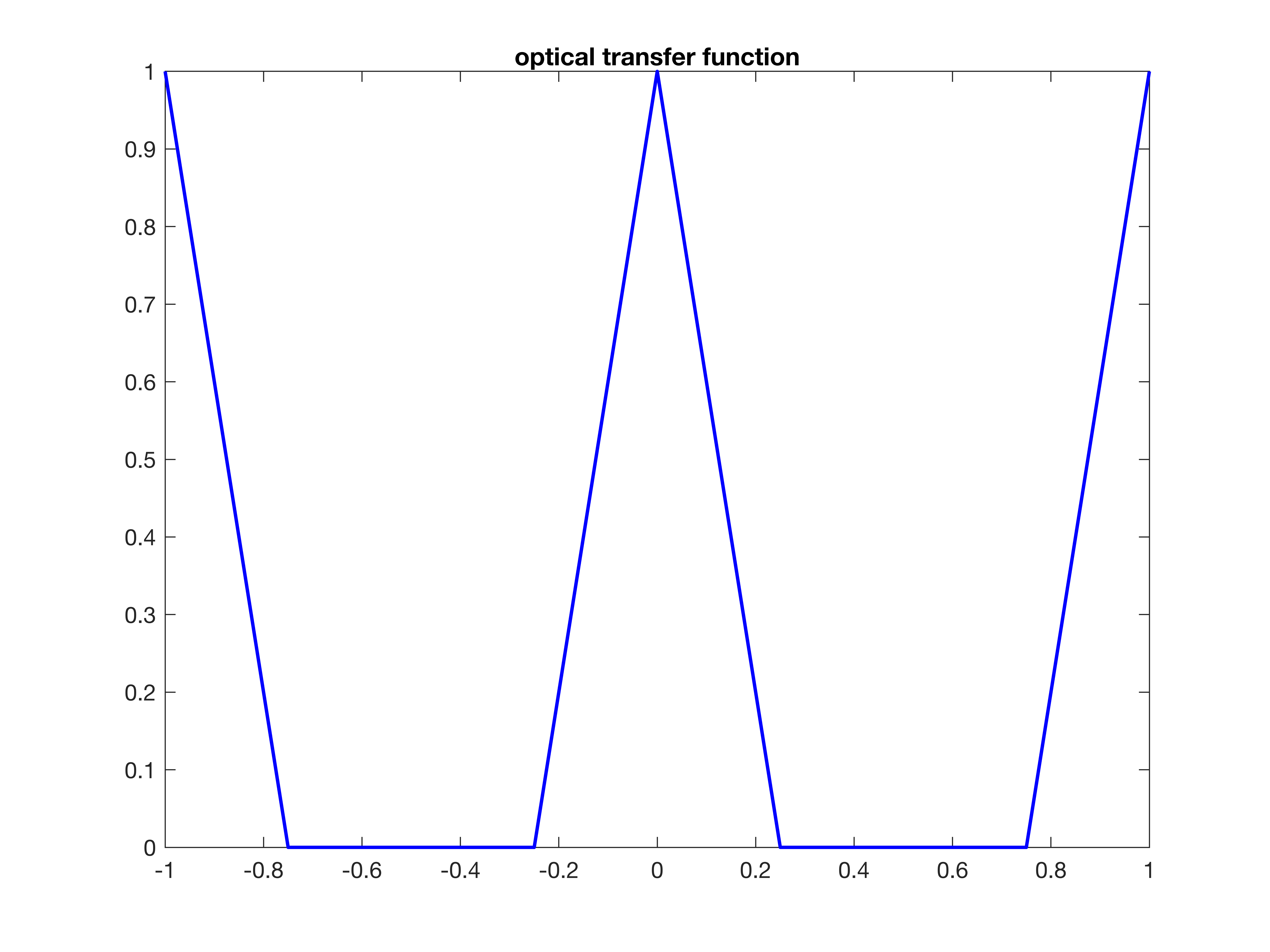
Figure 4.1: Optical transfer function.

5 Optimal Algorithms

We now have the exact resolution limit for determining whether the image is generated by one or two sources. This is a new benchmark for super-resolution and model order detection algorithms. A natural question is whether we can find the optimal algorithm to distinguish between one and two sources in the image. Note that, according to our theoretical results, when the two sources are separated by more than

$$\left|{y_{1}-y_{2}}\right|\geq\frac{4\arcsin\left(\left(\frac{\sigma}{m_{\min}}\right)^{\frac{1}{2}}\right)}{\Omega},$$

any algorithm targeting certain solutions in the set of admissible measures provides a solution with more than one source. But we still cannot confirm that there is more than one source inside. Only by considering the sparest solution in the set of admissible measures can we confirm this fact. However, since $l_{0}$ minimization is intractable, this direction is still unrealistic and we resort to other means. In [25], a simple singular value thresholding-based algorithm was proposed to detect the source number. In this section, we consider a variant of it and theoretically demonstrate that the algorithm exactly attains the resolution limit.

5.1 An optimal algorithm for detecting two sources in dimension one

In [25], the authors proposed a number detection algorithm called sweeping singular value thresholding number detection algorithm. It determines the number of sources by thresholding the singular value of a Hankel matrix formulated from the measurement data. Here we consider a simple variant of it.

To be more specific, we first assemble the following Hankel matrix from the measurements (4.2), that is,

$$\mathbf{H}=\left(\begin{array}[]{cc}\mathbf{Y}(-\Omega)&\mathbf{Y}(0)\\ \mathbf{Y}(0)&\mathbf{Y}(\Omega)\end{array}\right).$$ (5.1)

We denote the singular value decomposition of $\mathbf{H}$ as

$$\mathbf{H}=\hat{U}\hat{\Sigma}\hat{U}^{*},$$

where $\hat{\Sigma}=\text{diag}(\hat{\sigma}_{1},\hat{\sigma}_{2})$ with the singular values $\hat{\sigma}_{1},\hat{\sigma}_{2}$ ordered in a decreasing manner. We then determine the source number by a thresholding of the singular values. We derive the following Theorem 5.1 for the threshold and the resolution of the algorithm.

Theorem 5.1.

Consider $\mu=\sum_{j=1}^{2}a_{j}\delta_{y_{j}},y_{j}\in\mathbb{R}$ and the measurement $\boldsymbol{\mathbf{Y}}$ in (4.2) that is generated from $\mu$. If the following separation condition is satisfied

$$\left|{y_{1}-y_{2}}\right|\geq\frac{4\arcsin\left(\left(\frac{\sigma}{m_{\min}}\right)^{\frac{1}{2}}\right)}{\Omega},$$ (5.2)

then we have

$$\hat{\sigma}_{2}>2\sigma$$ (5.3)

for $\hat{\sigma}_{2}$ being the minimum singular value of the matrix $\boldsymbol{\mathbf{H}}$ in (5.1). On the other hand, if there exists $\hat{\mu}$ consisting of only one source being a $\sigma$-admissible measure of  $\boldsymbol{\mathbf{Y}}$, then

$$\hat{\sigma}_{2}<2\sigma.$$ (5.4)

Proof.

Observe that $\mathbf{H}$ has the decomposition

$$\mathbf{H}=DAD^{\top}+\Delta,$$ (5.5)

where $A=\text{diag}(e^{-iy_{1}\Omega}a_{1},e^{-iy_{2}\Omega}a_{2})$ and $D=\big{(}\phi_{1}(e^{iy_{1}\Omega}),\phi_{1}(e^{iy_{2}\Omega})\big{)}$ with $\phi_{1}(\omega)$ being defined as $(1,\omega)^{\top}$ and

$$\Delta=\left(\begin{array}[]{cc}\mathbf{W}(-\Omega)&\mathbf{W}(0)\\ \mathbf{W}(0)&\mathbf{W}(\Omega)\end{array}\right).$$

We denote the singular values of $DAD^{\top}$ by $\sigma_{1},\sigma_{2}$.

We first estimate $\left|\left|{\Delta}\right|\right|_{2}$. We have

$$\max_{x_{1}^{2}+x_{2}^{2}=1}\left|\left|{\Delta(x_{1},x_{2})^{\top}}\right|\right|_{2}$$

$$= \max_{x_{1}^{2}+x_{2}^{2}=1}\sqrt{(x_{1}\boldsymbol{\mathbf{W}}(-\Omega)+x_{2}\boldsymbol{\mathbf{W}}(0))^{2}+(x_{1}\boldsymbol{\mathbf{W}}(0)+x_{2}\boldsymbol{\mathbf{W}}(\Omega))^{2}}$$

$$= \max_{x_{1}^{2}+x_{2}^{2}=1}\sqrt{\boldsymbol{\mathbf{W}}(0)^{2}+2x_{1}x_{2}\boldsymbol{\mathbf{W}}(0)(\boldsymbol{\mathbf{W}}(-\Omega)+\boldsymbol{\mathbf{W}}(\Omega))+x_{1}^{2}\boldsymbol{\mathbf{W}}(-\Omega)^{2}+x_{2}^{2}\boldsymbol{\mathbf{W}}(\Omega)^{2}}$$

$$< \max_{x_{1}^{2}+x_{2}^{2}=1}\sqrt{\sigma^{2}+4\sigma^{2}x_{1}x_{2}+(x_{1}^{2}+x_{2}^{2})\sigma^{2}}\quad\Big{(}\text{by the condition on the noise}\Big{)}$$

$$= 2\sigma.$$

Thus we have $||\Delta||_{2}<2\sigma$. By Weyl’s theorem, we have

$$|\hat{\sigma}_{j}-\sigma_{j}|\leq||\Delta||_{2}<2\sigma,j=1,2.$$ (5.6)

Now we estimate the minimum singular value of $DAD^{\top}$ in the presence of two sources. Denote $\sigma_{\min}(M)$ and $\lambda_{\min}(M)$ as respectively the minimum singular value and eigenvalue of matrix $M$. We have

$$\sigma_{\min}(DAD^{\top})\geq m_{\min}\sigma_{\min}(D)^{2}=m_{\min}\lambda_{\min}(DD^{*})=4m_{\min}\sin\left(\left|{\frac{y_{1}-y_{2}}{4}}\right|\Omega\right)^{2}.$$

Therefore, when (5.2) holds, $\sigma_{\min}(DAD^{\top})\geq 4\sigma$. This is $\sigma_{2}\geq 4\sigma$. Similarly, by Weyl’s theorem, $|\hat{\sigma}_{2}-\sigma_{2}|\leq||\Delta||_{2}$. Thus, $\hat{\sigma}_{2}\geq 4\sigma-||\Delta||_{2}>2\sigma$. Conclusion (5.3) follows.

On the other hand, note that if there exists $\hat{\mu}=\hat{a}_{1}\delta_{\hat{y}_{1}}$ consisting of one source being a $\sigma$-admissible measure of $\boldsymbol{\mathbf{Y}}$, we can substitute the $D$ in (5.5) by $\big{(}\phi_{1}(e^{i\hat{y}_{1}\Omega})\big{)}$ with the $\boldsymbol{\mathbf{W}}$ and $\Delta$ being modified. Now we have $\sigma_{2}=0$ and also $||\Delta||_{2}<2\sigma$. Thus by (5.6) we get $|\hat{\sigma}_{2}|\leq||\Delta||_{2}<2\sigma$ and prove (5.4). ∎

We summarize the algorithm in the following Algorithm 1. Note that in practical applications one can estimate a noise level although not tight and utilize our algorithm to detect the source number. By Theorem 5.1, for all estimated $\sigma$’s less than $\frac{m_{\min}}{2}$, our algorithm can achieve super-resolution.

Input: Noise level $\sigma$;

Input: Measurement: $\mathbf{Y}(\omega),\omega\in[-\Omega,\Omega]$;

1: Formulate the Hankel matrix

$$\boldsymbol{\mathbf{H}}=\begin{pmatrix}\mathbf{Y}(-\Omega)&\mathbf{Y}(0)\\ \mathbf{Y}(0)&\mathbf{Y}(\Omega)\end{pmatrix}$$

from measurement $\boldsymbol{\mathbf{Y}}(\omega)$;

2: Compute the singular value of $\mathbf{H}$ as $\hat{\sigma}_{1},\hat{\sigma}_{2}$ distributed in a decreasing manner;

3: If $\hat{\sigma}_{2}\geq 2\sigma$, determine source number $n=2$ and otherwise, determine $n=1$;

Return: $n$.

Algorithm 1 Singular-value-thresholding number detection algorithm

Numerical experiments:
We conduct many numerical experiments to elucidate the performance of Algorithm 1. We consider $\Omega=1$ and measurements $\boldsymbol{\mathbf{Y}}$ generated by two sources. The noise level is $\sigma$ and the minimum separation distance between sources is $d_{\min}$. We first perform $100000$ random experiments (the randomness is in the choice of $(d_{\min},\sigma,y_{j},a_{j})$) and the results were shown in Figure 5.1 (a)-(c). The green points and red points represent respectively the cases of successful detection and failed detection. It is indicated that in many cases, our Algorithm 1 can surpass the diffraction limit. We also conduct $100000$ experiments for the worst-case scenario; see results in Figure 5.1 (d)-(f). As shown numerically, our algorithm successfully detects the source number when $d_{\min}$ is above the diffraction limit and failed in exactly the opposite cases. Last, we consider the worst cases when detecting the source number is impossible when $\frac{\sigma}{m_{\min}}>\frac{1}{2}$. The results were presented in Figure 5.1 (g)-(i) and there is no successful case when $\frac{\sigma}{m_{\min}}>\frac{1}{2}$. Note that the failed cases when $\frac{\sigma}{m_{\min}}<\frac{1}{2}$ and $d_{\min}$ above the diffraction limit is due to the fact that $|e^{iy_{1}\Omega}-e^{iy_{2}\Omega}|$ becomes small when $|y_{1}-y_{2}|\Omega$ approaching $2\pi$.

We also conduct several experiments to illustrate that our algorithm can detect the correct source number even if it seems very unlikely to distinguish the two sources by other methods. We consider $5$ cases where the source number is correctly detected by our algorithm; see Figure 5.2 (a). However, as shown by Figure 5.2 (b)-(f), their MUSIC images only have one peak.

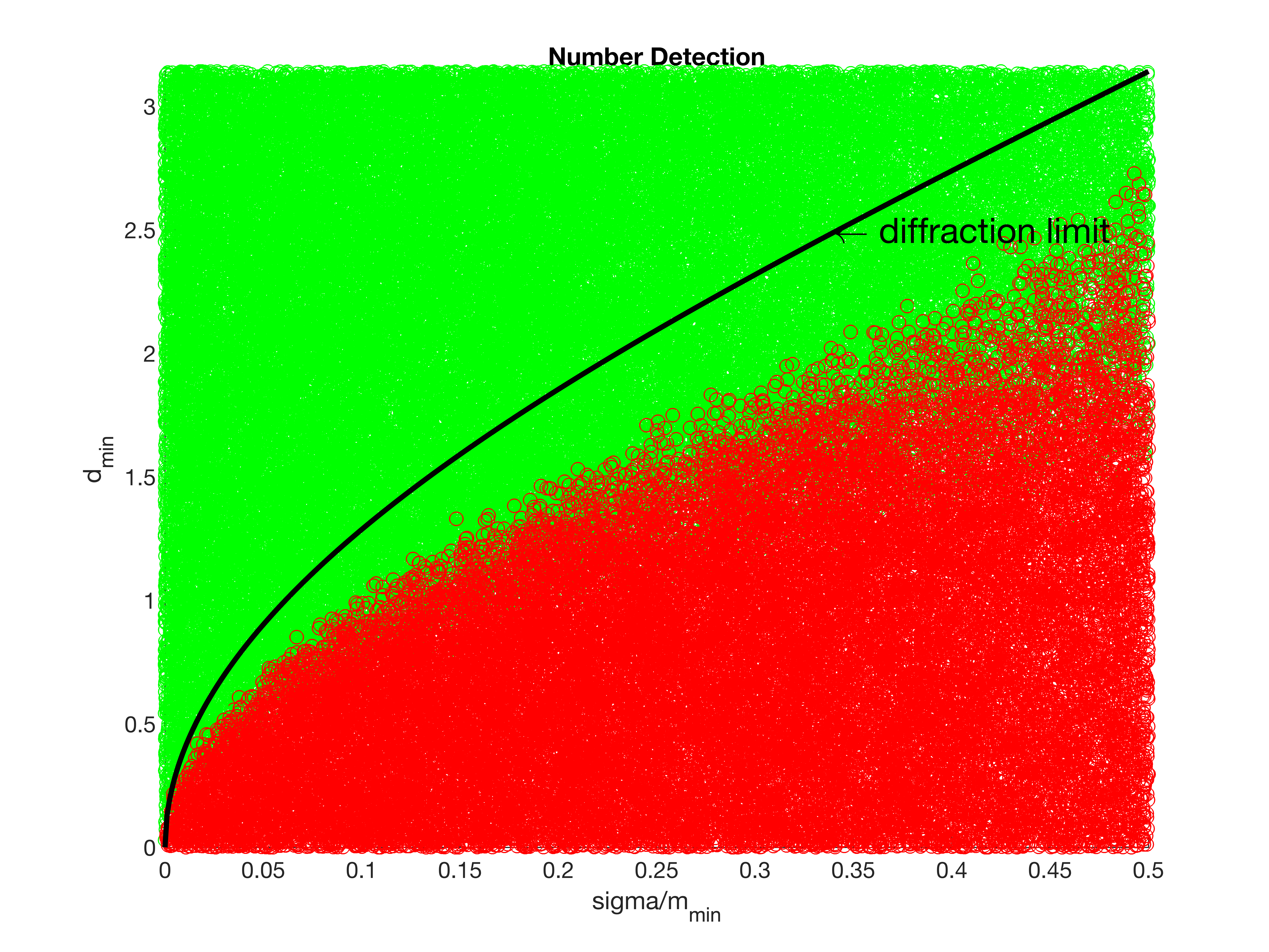
(a) detection results

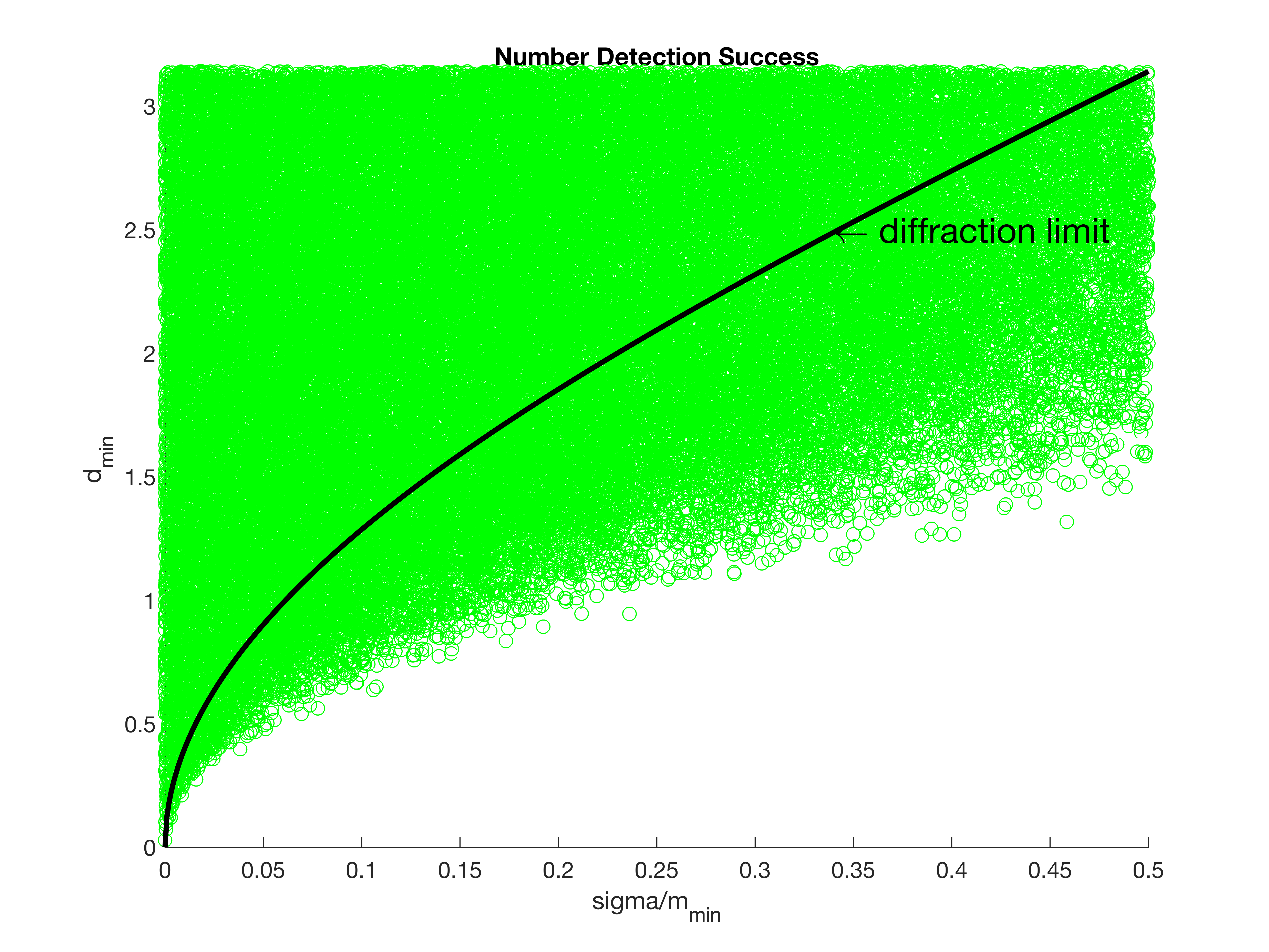
(b) detection success

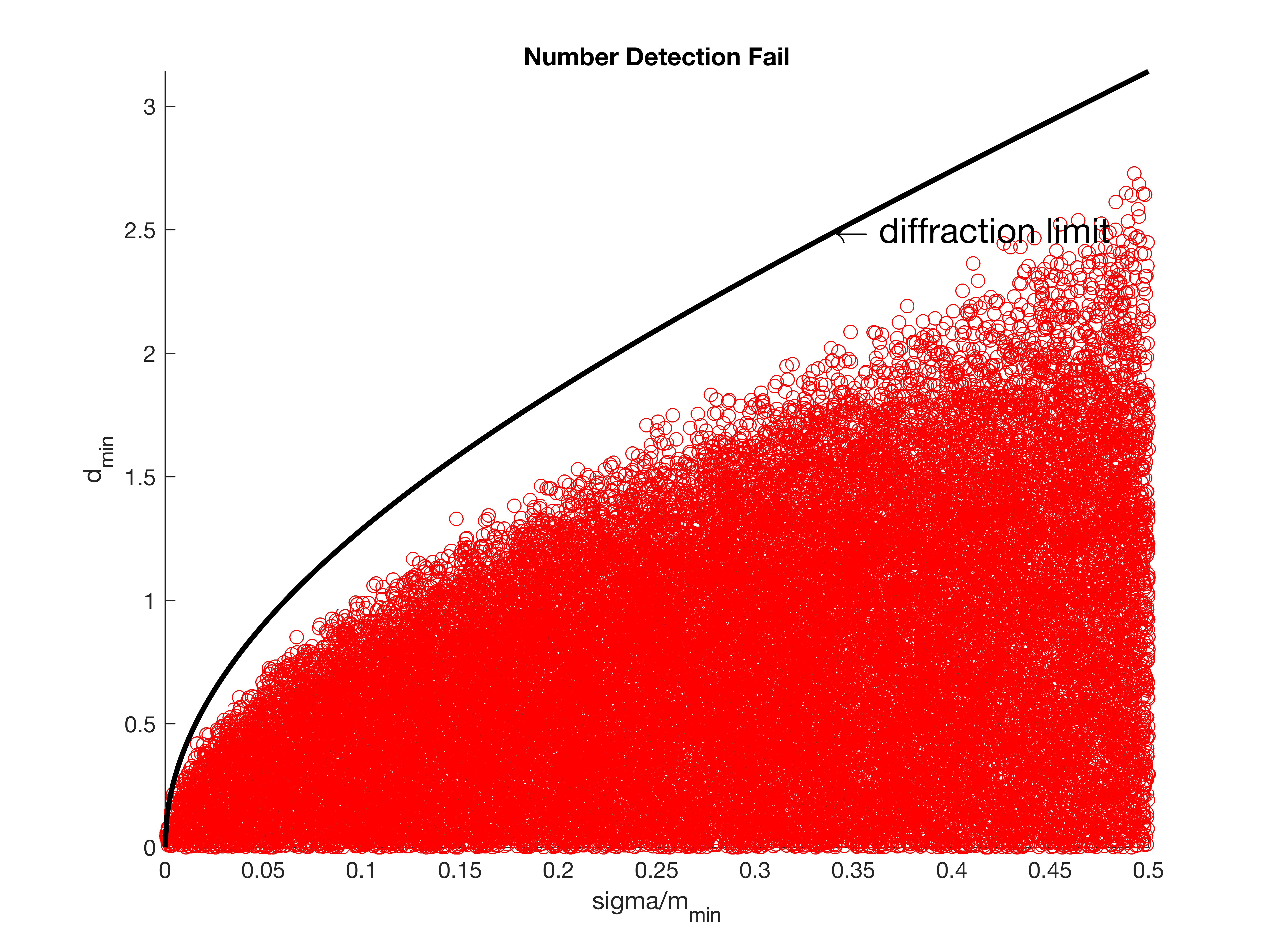
(c) detection fail

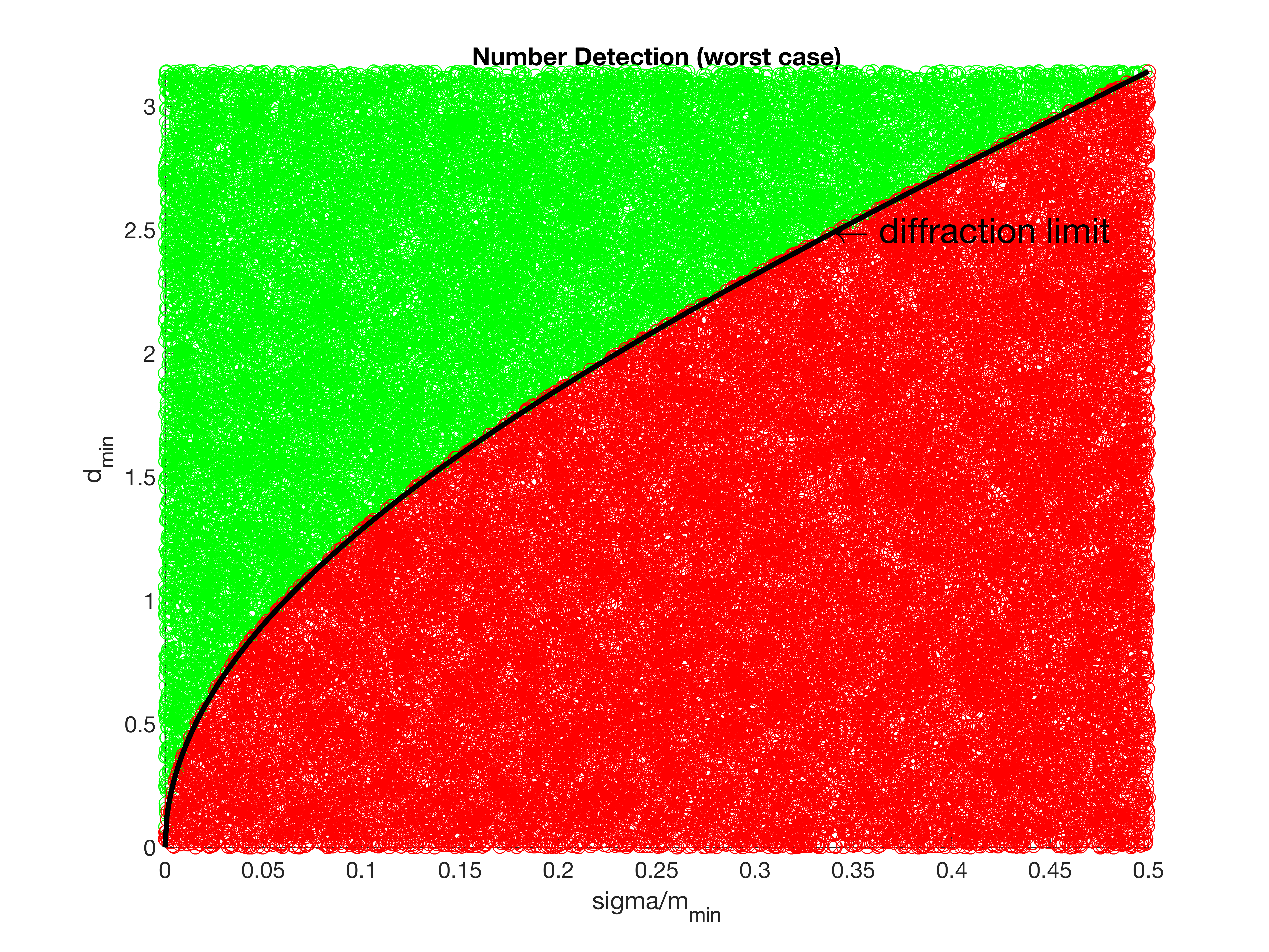
(d) detection results

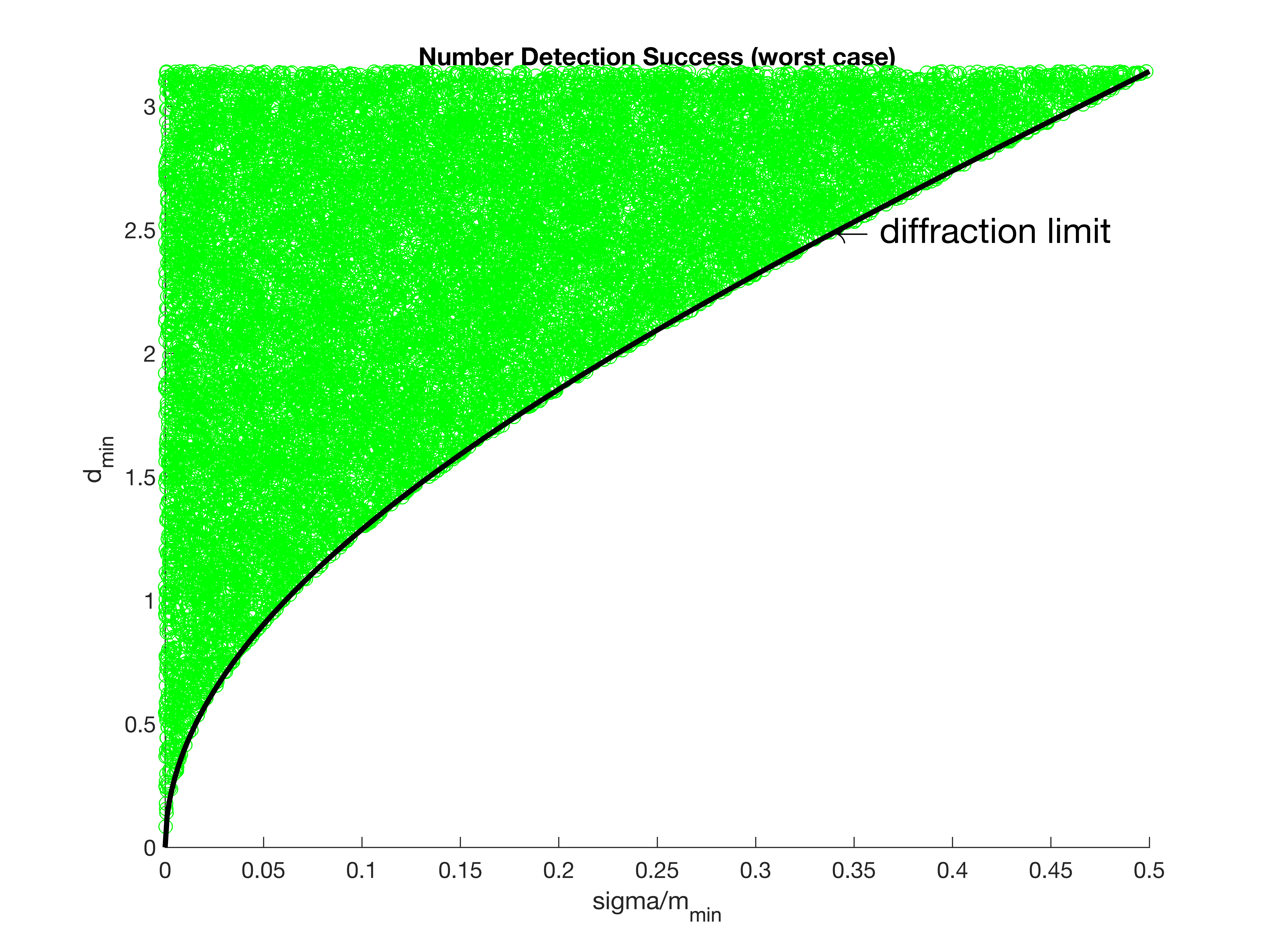
(e) detection success

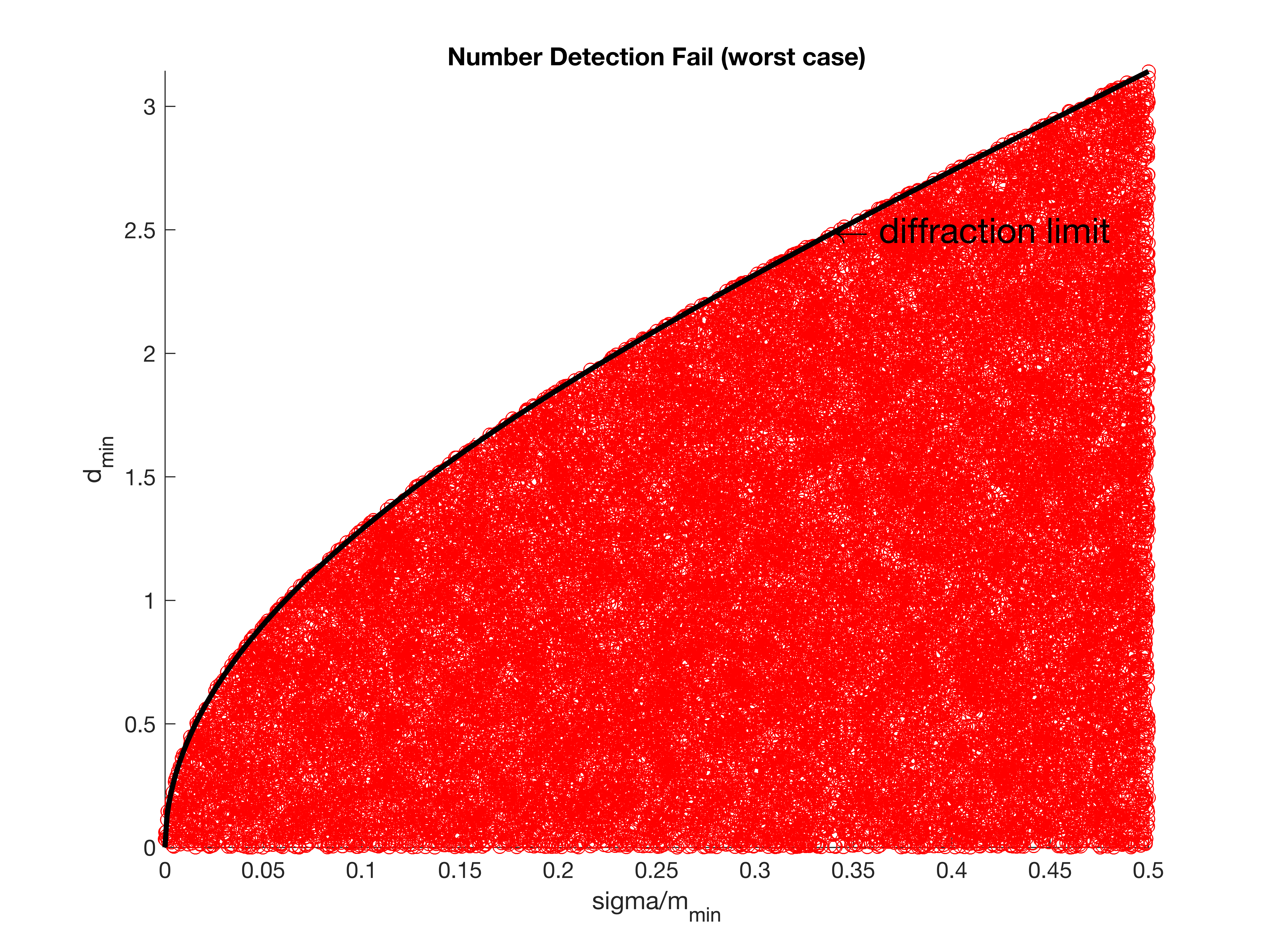
(f) detection fail

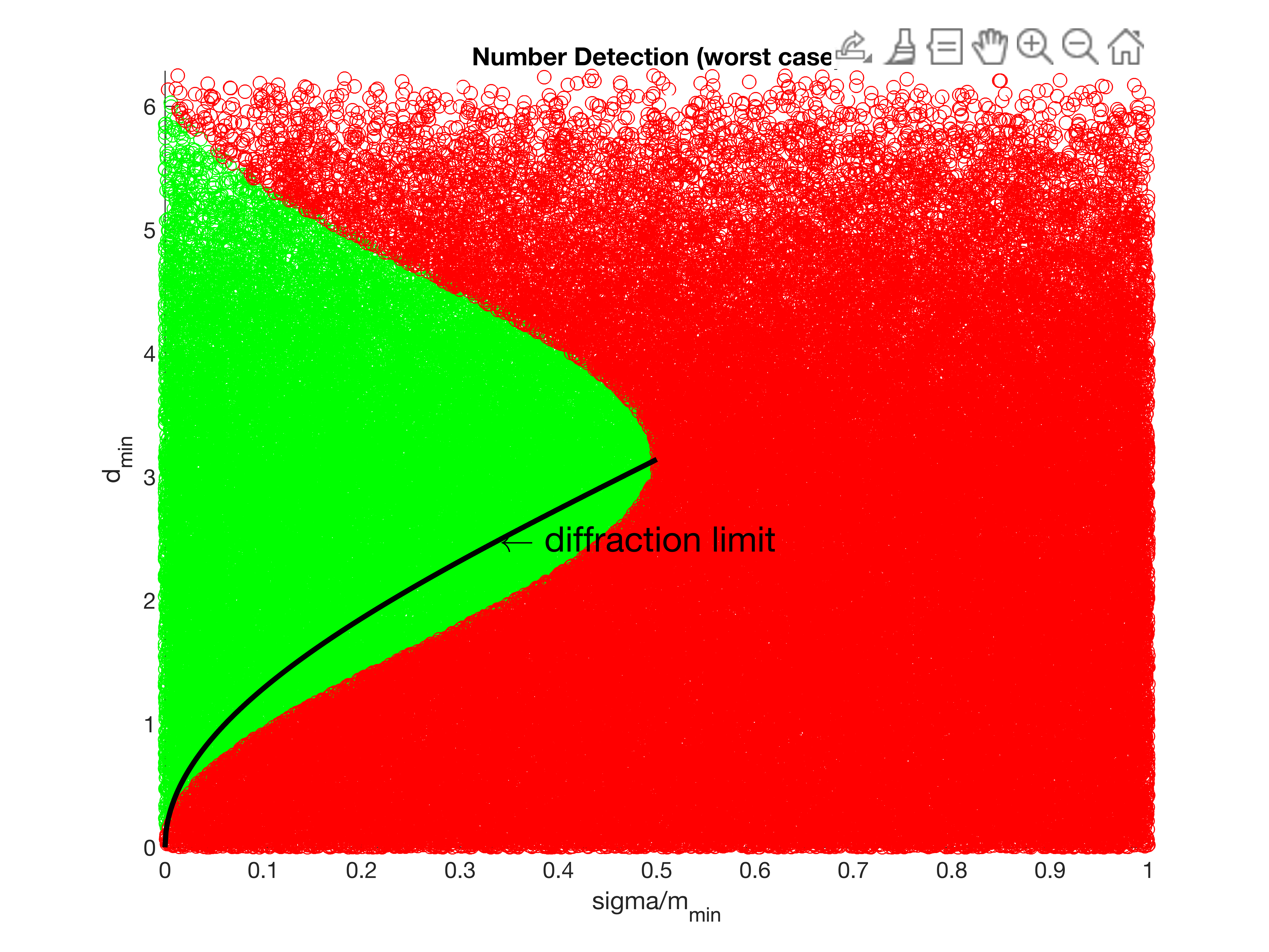
(g) detection results

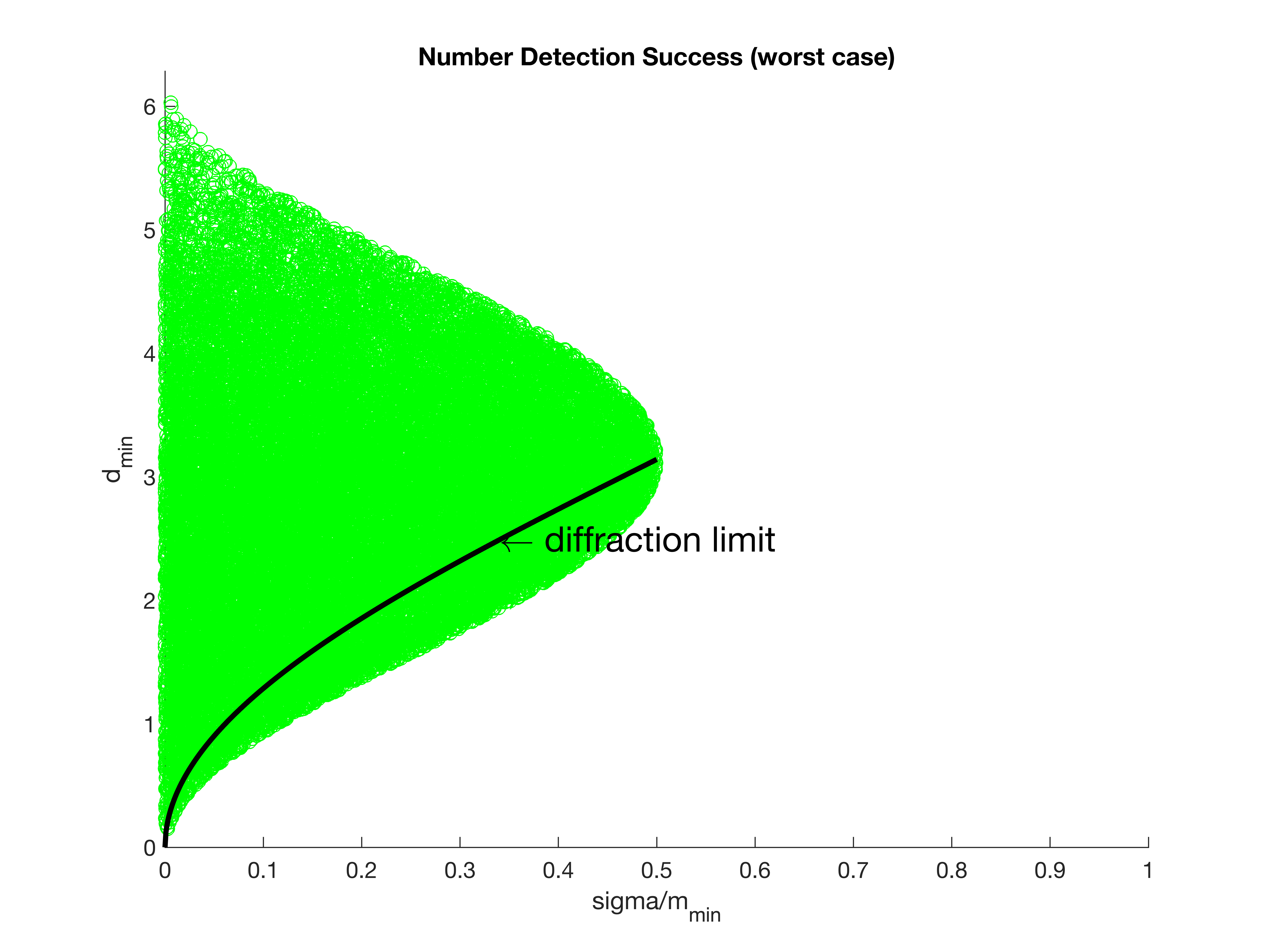
(h) detection success

(i) detection fail

Figure 5.1: Plots of the successful and the unsuccessful number detections by Algorithm 1 depending on the relation between $\frac{\sigma}{m_{\min}}$ and $d_{\min}$. The green points and red points represent respectively the cases of successful detection and failed detection. The black line is the diffraction limit derived in Theorem 4.1.

(a) detection results

(b) MUSIC image

(c) MUSIC image

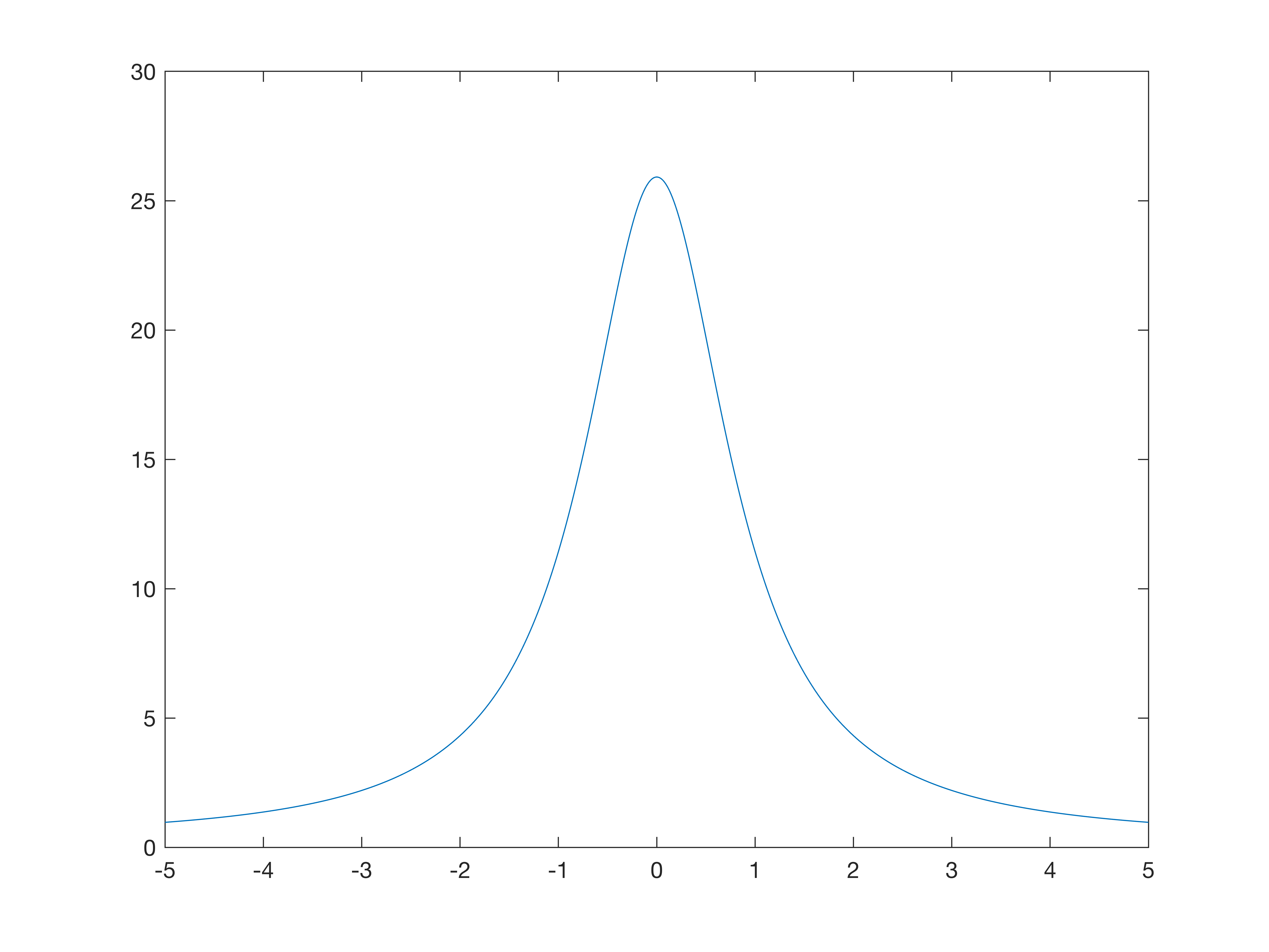
(d) MUSIC image

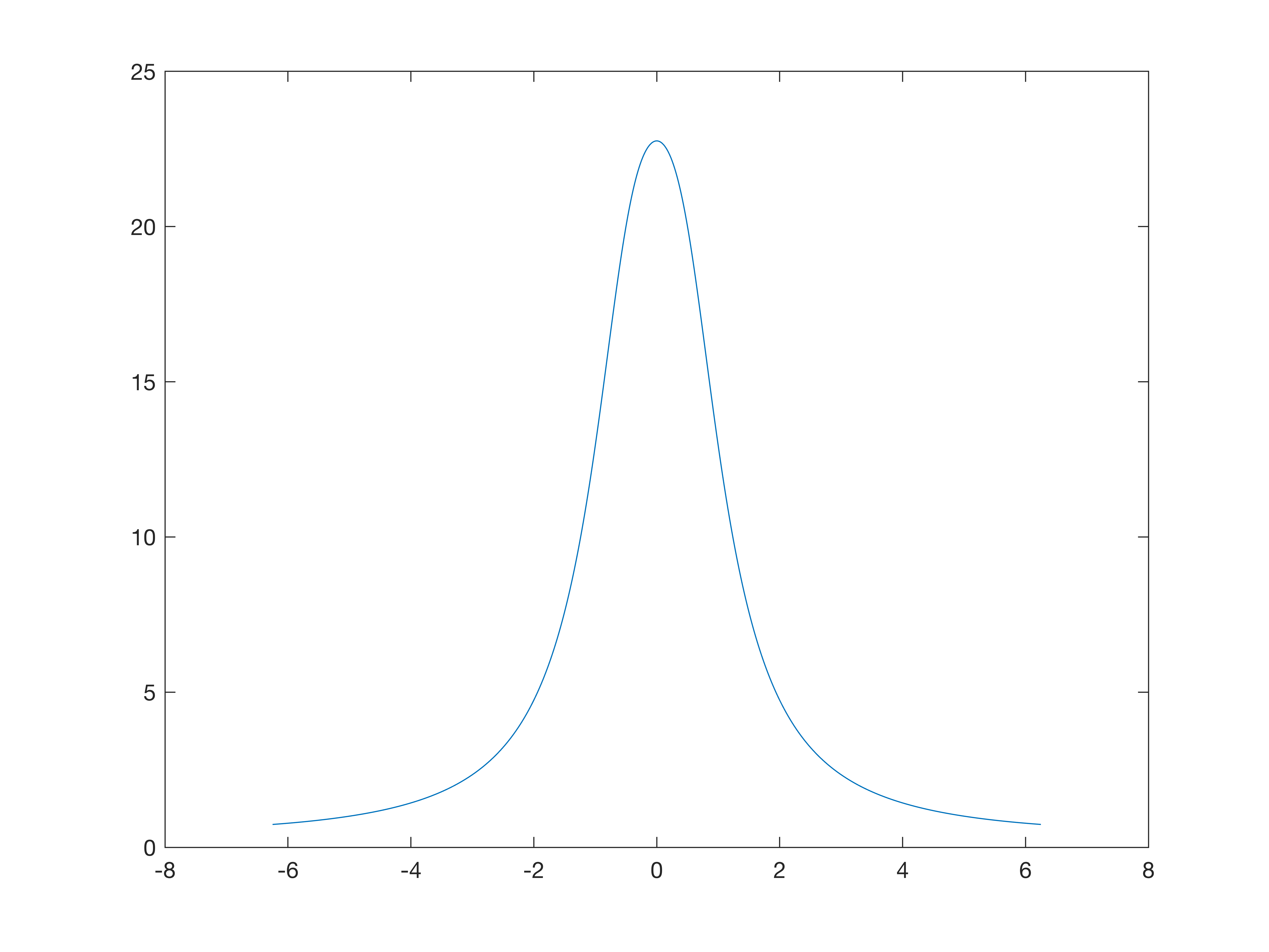
(e) MUSIC image

(f) MUSIC image

Figure 5.2: Plot (a) is the relation between $\frac{\sigma}{m_{\min}}$ and $d_{\min}$ for several cases. Plots (b)-(f) are MUSIC images of these cases. Note that it is impossible to detect the correct source number from these MUSIC images.

5.2 An optimal algorithm for detecting two sources in multi-dimensional spaces

For detecting two sources in multi-dimensional spaces, we can first apply Algorithm 1 to the measurement in several one-dimensional subspaces $V_{j}$’s and save the outputs, then determine the source number as the maximum value among these outputs. If some of the $V_{j}$’s are sufficiently close to the space spanned by $\boldsymbol{\mathbf{y}}_{2}-\boldsymbol{\mathbf{y}}_{1}$, it actually achieves similar resolution to the one in Theorem 5.1.

To be specific, let $\mu=\sum_{j=1}^{2}a_{j}\delta_{\boldsymbol{\mathbf{y}}_{j}},\boldsymbol{\mathbf{y}}_{j}\in\mathbb{R}^{k}$ and $\boldsymbol{\mathbf{Y}}(\boldsymbol{\mathbf{\omega}}),\boldsymbol{\mathbf{\omega}}\in\mathbb{R}^{k},||\boldsymbol{\mathbf{\omega}}||_{2}\leq\Omega$ be the associated measurement in (4.2). We choose $N$ unit vectors $\boldsymbol{\mathbf{v}}_{j}$’s in $\mathbb{R}^{k}$ and formulate the corresponding Hankel matrices $\boldsymbol{\mathbf{H}}_{q}$’s as

$$\mathbf{H}_{q}=\left(\begin{array}[]{cc}\mathbf{Y}(-\Omega\boldsymbol{\mathbf{v}}_{q})&\mathbf{Y}(0)\\ \mathbf{Y}(0)&\mathbf{Y}(\Omega\boldsymbol{\mathbf{v}}_{q})\end{array}\right),\quad q=1,\cdots,N.$$ (5.7)

Denoting $\hat{\sigma}_{q,j}$ the $j$-th singular value of $\boldsymbol{\mathbf{H}}_{q}$, we can detect the source number by thresholding on $\hat{\sigma}_{q,j}$’s. Moreover, we have the following theorem on the resolution and the threshold.

Theorem 5.2.

Consider $\mu=\sum_{j=1}^{2}a_{j}\delta_{\boldsymbol{\mathbf{y}}_{j}},\boldsymbol{\mathbf{y}}_{j}\in\mathbb{R}^{k}$ and the measurement $\boldsymbol{\mathbf{Y}}$ in (4.2) that is generated from $\mu$. If

$$\min_{q=1,\cdots,N}\min\left(\left|\angle(\boldsymbol{\mathbf{y}}_{1}-\boldsymbol{\mathbf{y}}_{2},\boldsymbol{\mathbf{v}}_{q})\right|,\ \pi-\left|\angle(\boldsymbol{\mathbf{y}}_{1}-\boldsymbol{\mathbf{y}}_{2},\boldsymbol{\mathbf{v}}_{q})\right|\right)=\theta_{\min}$$ (5.8)

with $\angle(\cdot,\cdot)$ denoting the angle between vectors, and the following separation condition is satisfied

$$\left|\left|{\boldsymbol{\mathbf{y}}_{1}-\boldsymbol{\mathbf{y}}_{2}}\right|\right|_{2}\geq\frac{4\arcsin\left(\left(\frac{\sigma}{m_{\min}}\right)^{\frac{1}{2}}\right)}{\Omega\cos{\theta_{\min}}},$$ (5.9)

then we have

$$\max_{q=1,\cdots,N}\hat{\sigma}_{q,2}>2\sigma$$ (5.10)

for $\hat{\sigma}_{q,2}$ being the minimum singular value of the Hankel matrix $\boldsymbol{\mathbf{H}}_{q}$ that defined in (5.7). On the other hand, if there exists $\hat{\mu}$ consisting of only one source being the a $\sigma$-admissible measure of  $\boldsymbol{\mathbf{Y}}$, then

$$\hat{\sigma}_{q,2}<2\sigma,\quad q=1,\cdots,N.$$ (5.11)

Proof.

By (5.8), there exists $\boldsymbol{\mathbf{v}}_{q^{*}}$ such that

$$\left|{\boldsymbol{\mathbf{y}}_{1}\cdot\boldsymbol{\mathbf{v}}_{q^{*}}-\boldsymbol{\mathbf{y}}_{2}\cdot\boldsymbol{\mathbf{v}}_{q^{*}}}\right|=\cos\theta_{\min}\left|\left|{\boldsymbol{\mathbf{y}}_{1}-\boldsymbol{\mathbf{y}}_{2}}\right|\right|_{2}\geq\frac{4\arcsin\left(\left(\frac{\sigma}{m_{\min}}\right)^{\frac{1}{2}}\right)}{\Omega}.$$

Hence, similar to the proof of Theorem 5.1, we can show that $\hat{\sigma}_{q^{*},2}>2\sigma$. This proves (5.9). Also, we can show (5.11) in the same way as the one in the proof of Theorem 5.1. ∎

We summarize the algorithm as the following Algorithm 2.

Input: Noise level $\sigma$, measurement: $\mathbf{Y}(\boldsymbol{\mathbf{\omega}}),\boldsymbol{\mathbf{\omega}}\in\mathbb{R}^{k},||\boldsymbol{\mathbf{\omega}}||_{2}\leq\Omega$;

Input: $N$ unit vectors $\boldsymbol{\mathbf{v}}_{q}$’s;

for $q=1,\cdots,N$ do

       Formulate the Hankel matrix:

$$\mathbf{H}_{q}=\left(\begin{array}[]{cc}\mathbf{Y}(-\Omega\boldsymbol{\mathbf{v}}_{q})&\mathbf{Y}(0)\\ \mathbf{Y}(0)&\mathbf{Y}(\Omega\boldsymbol{\mathbf{v}}_{q})\end{array}\right).$$

Compute the singular value of $\mathbf{H}$ as $\hat{\sigma}_{1},\hat{\sigma}_{2}$ distributed in a decreasing manner;

       if $\hat{\sigma}_{2}\geq 2\sigma$ then

            Return $n=2$.

      

Return $n=1$.

Algorithm 2 Multi-dimensional singular-value-thresholding number detection algorithm

Numerical experiments:
We consider detecting two sources in two-dimensional spaces. For large enough $N$, we consider

$$\boldsymbol{\mathbf{v}}_{q}=\left(\cos\left(\frac{q\pi}{N}\right),\ \sin\left(\frac{q\pi}{N}\right)\right)^{\top}\in\mathbb{R}^{2},\quad q=1,\cdots,N.$$ (5.12)

Input $\boldsymbol{\mathbf{v}}_{q}$’s to Algorithm 2, we then determine the source number by Algorithm 2 from measurements $\boldsymbol{\mathbf{Y}}(\boldsymbol{\mathbf{\omega}})$. By Theorem 5.2, we can determine the correct number when

$$\left|\left|{\boldsymbol{\mathbf{y}}_{1}-\boldsymbol{\mathbf{y}}_{2}}\right|\right|_{2}\geq\frac{4\arcsin\left(\left(\frac{\sigma}{m_{\min}}\right)^{\frac{1}{2}}\right)}{\Omega\cos\left({\frac{\pi}{2N}}\right)}.$$

This indicates that we already have an excellent resolution by leveraging only a few $\boldsymbol{\mathbf{v}}_{q}$’s. We use $N=10$ unit vectors in the experiments and conduct $100000$ random experiments for both the general and worst cases. As shown in Figure 5.3 (a) and (c), our algorithm successfully detects the source number when $d_{\min}$ is above nearly the diffraction limit and fails to detect the source number on some cases when $d_{\min}$ is below the diffraction limit. A very interesting phenomenon is that, as shown in Figure 5.3 (b), there are many cases in which our algorithm detects the correct source number even when $d_{\min}$ is much lower than the diffraction limit. This indicates that the tolerance of the noise of the algorithm is in fact excellent. The reason is that the worst cases or nearly worst cases actually only happen when the noise satisfies certain patterns. Because we use the measurements in $N$ one-dimensional subspaces, it becomes more difficult for the noises in all the subspaces to satisfy these patterns. Thus the noise tolerance becomes better in the two-dimensional case.

Note that our theoretical results and algorithms are potentially of great importance in practical applications. We will examine the super-resolving ability of our algorithm in practical examples in a future work.

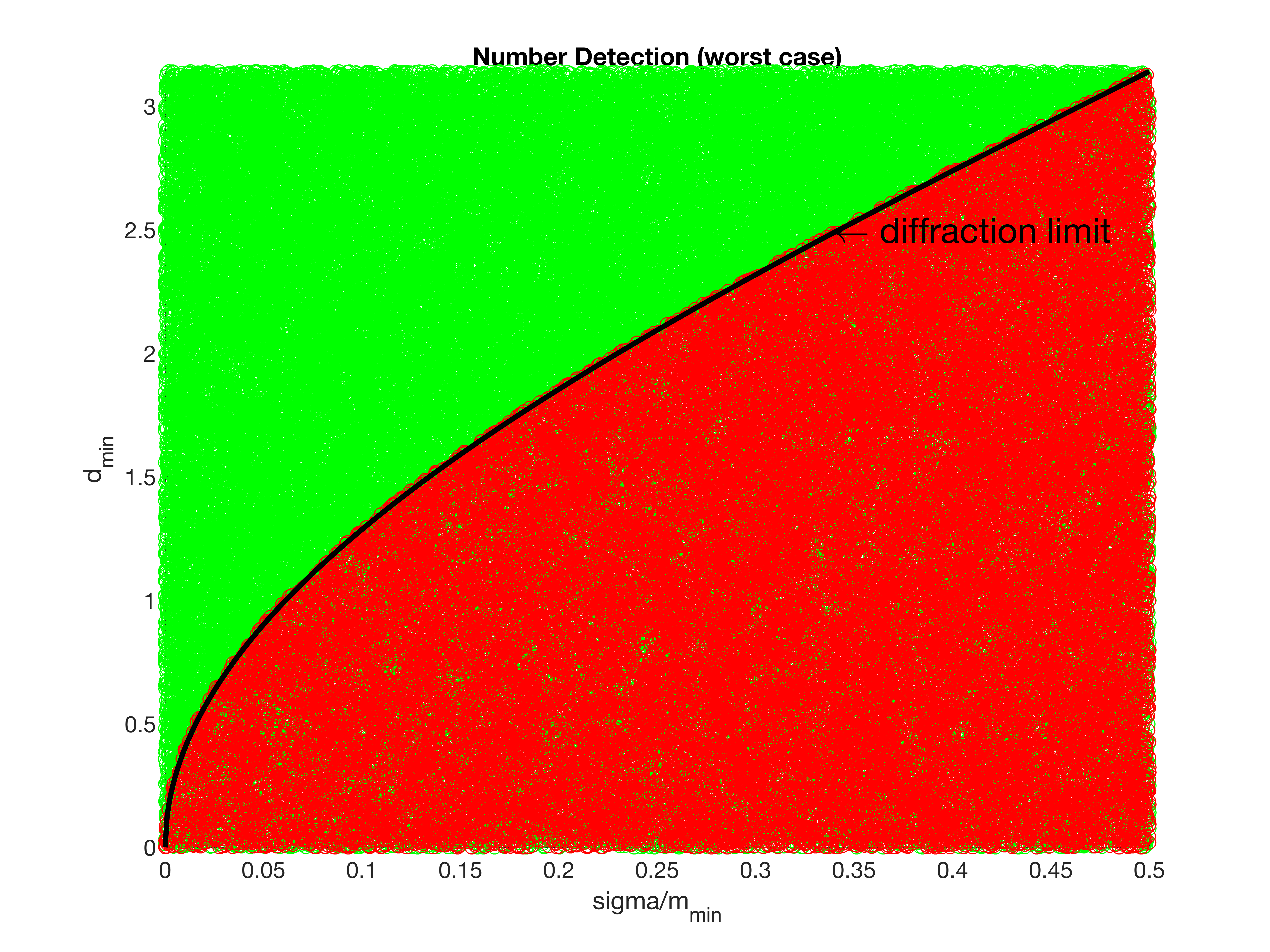
(a) detection results

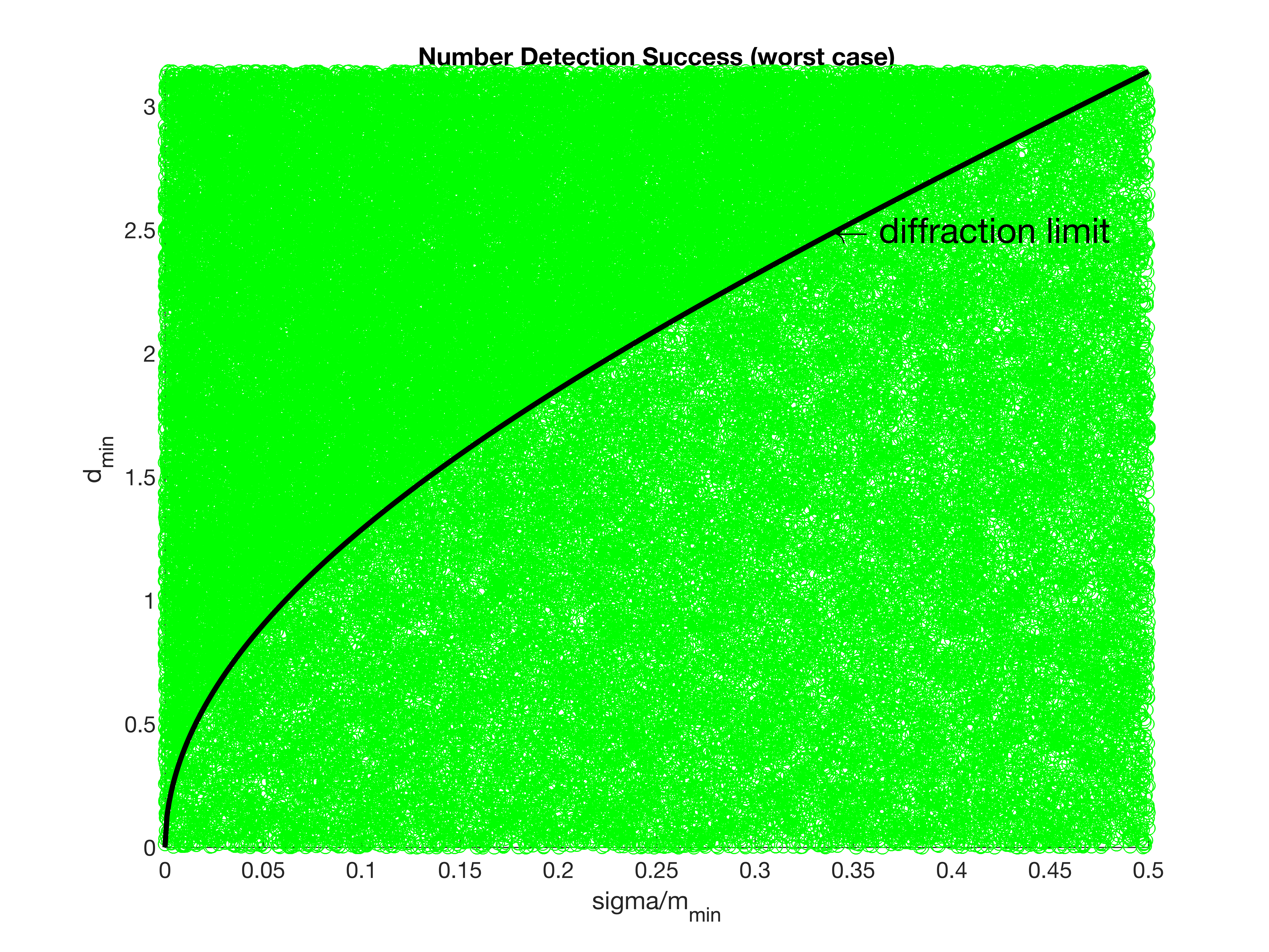
(b) detection success

(c) detection fail

Figure 5.3: Plots of the successful and the unsuccessful number detections by Algorithm 2 depending on the relation between $\frac{\sigma}{m_{\min}}$ and $d_{\min}$. The green points and red points represent respectively the cases of successful detection and failed detection. The black line is the diffraction limit derived in Theorem 4.1.

Appendix A Some inequalities

In this Appendix, we present some inequalities that are used in this paper. We first recall the following Stirling approximation of factorial

$$\sqrt{2\pi}n^{n+\frac{1}{2}}e^{-n}\leq n!\leq en^{n+\frac{1}{2}}e^{-n},$$ (A.1)

which will be used frequently in the subsequent derivations.

Lemma A.1.

Let $\zeta(n)$ and $\xi(n-1)$ be defined as in (3.4). For $n\geq 2$, we have

$$\Big{(}\frac{2}{\zeta(n)\xi(n-1)}\Big{)}^{\frac{1}{2n-2}}\leq\frac{2e}{n-1}.$$

Proof.

For $n=2,3,4$, it is easy to check that the above inequality holds. Using (A.1), we have for odd $n\geq 5$,

$$\zeta(n)\xi(n-1)=(\frac{n-1}{2}!)^{2}\frac{(\frac{n-3}{2}!)^{2}}{4}\geq\pi^{2}(\frac{n-1}{2})^{n}(\frac{n-3}{2})^{n-2}e^{-(2n-4)}$$

$$= (n-1)^{n-2}\frac{\pi^{2}(\frac{n-1}{2})^{n}(\frac{n-3}{2})^{n-2}e^{-(2n-4)}}{(n-1)^{n-2}}$$

$$= \pi^{2}e^{2}\left(\frac{n-1}{2e}\right)^{2n-2}\frac{(n-3)^{n-2}}{(n-2)^{n-2}}$$

$$\geq 0.29\pi^{2}e^{2}\left(\frac{n-1}{2e}\right)^{2n-2}\quad\Big{(}\text{since $n\geq 5$}\Big{)}$$

and for even $n\geq 6$,

$$\zeta(n)\xi(n-1)=(\frac{n}{2})!(\frac{n-2}{2})!\frac{(\frac{n-2}{2})!(\frac{n-4}{2})!}{4}$$

$$\geq \pi^{2}(\frac{n}{2})^{\frac{n+1}{2}}(\frac{n-2}{2})^{n-1}(\frac{n-4}{2})^{\frac{n-3}{2}}e^{-(2n-4)}$$

$$= (n-1)^{2n-2}\frac{\pi^{2}(\frac{n}{2})^{\frac{n+1}{2}}(\frac{n-2}{2})^{n-1}(\frac{n-4}{2})^{\frac{n-3}{2}}e^{-(2n-4)}}{(n-1)^{2n-2}}$$

$$= \pi^{2}e^{2}\left(\frac{n-1}{2e}\right)^{2n-2}\frac{n^{\frac{n+1}{2}}(n-2)^{n-1}(n-4)^{\frac{n-3}{2}}}{(n-1)^{2n-2}}$$

$$> \pi^{2}\left(\frac{n-1}{2e}\right)^{2n-2}.$$

Therefore, for all $n\geq 5$,

$$\Big{(}\frac{2}{\zeta(n)\xi(n-1)}\Big{)}^{\frac{1}{2n-2}}\leq\frac{2e}{n-1}\Big{(}\frac{2}{\pi^{2}}\Big{)}^{\frac{1}{2n-2}}\leq\frac{2e}{n-1}.$$

∎

Lemma A.2.

Let $\zeta(n)$ and $\lambda(n)$ be defined as in (3.4) and (3.16), respectively. For $n\geq 2$, we have

$$\Big{(}\frac{8}{\zeta(n)\lambda(n)}\Big{)}^{\frac{1}{2n-1}}\leq\frac{2.36e}{n-\frac{1}{2}}.$$

Proof.

For $n=2,3,4,5$, the inequality follows from direct calculation. By the Stirling approximation (A.1), we have for even $n\geq 6$,

$$\zeta(n)\lambda(n)=\zeta(n)\xi(n-2)=(\frac{n}{2})!(\frac{n-2}{2})!\frac{(\frac{n-4}{2}!)^{2}}{4}$$

$$\geq \pi^{2}(\frac{n}{2})^{\frac{n+1}{2}}(\frac{n-2}{2})^{\frac{n-1}{2}}(\frac{n-4}{2})^{n-3}e^{-(2n-5)}$$

$$= (n-\frac{1}{2})^{2n-1}\frac{\pi^{2}(\frac{n}{2})^{\frac{n+1}{2}}(\frac{n-2}{2})^{\frac{n-1}{2}}(\frac{n-4}{2})^{n-3}e^{-(2n-5)}}{(n-\frac{1}{2})^{2n-1}}$$

$$= (\frac{n-\frac{1}{2}}{2e})^{2n-1}\frac{\pi^{2}e^{4}2^{2}}{(n-\frac{1}{2})^{2}}\frac{n^{\frac{n+1}{2}}(n-2)^{\frac{n-1}{2}}(n-4)^{n-3}}{(n-\frac{1}{2})^{2n-3}}$$

$$\geq (\frac{n-\frac{1}{2}}{2e})^{2n-1}\frac{4\pi^{2}}{(n-\frac{1}{2})^{2}},$$

and for odd $n\geq 7$,

$$\zeta(n)\lambda(n)=\zeta(n)\xi(n-2)=(\frac{n-1}{2}!)^{2}\frac{(\frac{n-3}{2})!(\frac{n-5}{2})!}{4}$$

$$\geq \pi^{2}(\frac{n-1}{2})^{n}(\frac{n-3}{2})^{\frac{n-2}{2}}(\frac{n-5}{2})^{\frac{n-4}{2}}e^{-(2n-5)}$$

$$= (n-\frac{1}{2})^{2n-1}\frac{\pi^{2}(\frac{n-1}{2})^{n}(\frac{n-3}{2})^{\frac{n-2}{2}}(\frac{n-5}{2})^{\frac{n-4}{2}}e^{-(2n-5)}}{(n-\frac{1}{2})^{2n-1}}$$

$$= (\frac{n-\frac{1}{2}}{2e})^{2n-1}\frac{\pi^{2}e^{4}2^{2}}{(n-\frac{1}{2})^{2}}\frac{(n-1)^{n}(n-3)^{\frac{n-2}{2}}(n-5)^{\frac{n-4}{2}}}{(n-\frac{1}{2})^{2n-3}}$$

$$\geq (\frac{n-\frac{1}{2}}{2e})^{2n-1}\frac{4\pi^{2}}{(n-\frac{1}{2})^{2}}.$$

Therefore, for all $n\geq 6$,

$$\Big{(}\frac{8}{\zeta(n)\lambda(n)}\Big{)}^{\frac{1}{2n-1}}\leq\frac{2e}{n-\frac{1}{2}}\Big{(}\frac{(n-\frac{1}{2})^{2}8}{4\pi^{2}}\Big{)}^{\frac{1}{2n-1}}\leq\frac{2.36e}{n-\frac{1}{2}}.$$

∎

Lemma A.3.

Let $\zeta(n)$ be defined as in (3.4). For $n\geq 2$, we have

$$\frac{(n-\frac{1}{2})^{2n-2}}{\zeta(n)(n-2)!}\leq\frac{2^{n-\frac{3}{2}}e^{2n-1}}{(\sqrt{\pi})^{3}\max(\sqrt{n-2},1)}.$$

Proof: By the Stirling approximation formula (A.1), when $n$ is odd and $n\geq 3$, we have

$$\frac{(n-\frac{1}{2})^{2n-2}}{\zeta(n)(n-2)!}=\frac{(n-\frac{1}{2})^{2n-2}}{(\frac{n-1}{2}!)^{2}(n-2)!}$$

$$\leq \frac{(n-\frac{1}{2})^{2n-{2}}}{(\sqrt{2\pi})^{3}(\frac{n-1}{2})^{n}(n-2)^{n-2+\frac{1}{2}}e^{-(2n-3)}}$$

$$\leq \frac{2^{n}e^{2n}}{(e\sqrt{2\pi})^{3}\sqrt{n-2}}\frac{(n-\frac{1}{2})^{2n-{2}}}{(n-1)^{n}(n-2)^{n-{2}}}\leq\frac{2^{n-\frac{3}{2}}e^{2n-1}}{(\sqrt{\pi})^{3}\sqrt{n-2}}.$$

When $n$ is even and $n\geq 4$, we have

$$\frac{(n-\frac{1}{2})^{2n-{2}}}{\zeta(n)(n-2)!}=\frac{(n-\frac{1}{2})^{2n-{2}}}{(\frac{n}{2})!(\frac{n-2}{2})!(n-2)!}$$

$$\leq \frac{(n-\frac{1}{2})^{2n-{2}}}{(\sqrt{2\pi})^{3}(\frac{n}{2})^{\frac{n+1}{2}}(\frac{n-2}{2})^{\frac{n-1}{2}}(n-2)^{n-2+\frac{1}{2}}e^{-(2n-3)}}$$

$$\leq \frac{2^{n}e^{2n}}{(e\sqrt{2\pi})^{3}\sqrt{n-2}}\frac{(n-\frac{1}{2})^{2n-{2}}}{n^{\frac{n+1}{2}}(n-2)^{\frac{n-1}{2}}(n-2)^{n-{2}}}\leq\frac{2^{n-\frac{3}{2}}e^{2n-1}}{(\sqrt{\pi})^{3}\sqrt{n-2}}.$$

For $n=2$, the inequality follows from a direct calculation.

References

- [1] Ernst Abbe. Beiträge zur theorie des mikroskops und der mikroskopischen wahrnehmung. Archiv für mikroskopische Anatomie, 9(1):413–468, 1873.
- [2] Dmitry Batenkov, Laurent Demanet, Gil Goldman, and Yosef Yomdin. Conditioning of partial nonuniform fourier matrices with clustered nodes. SIAM Journal on Matrix Analysis and Applications, 41(1):199–220, 2020.
- [3] Dmitry Batenkov, Gil Goldman, and Yosef Yomdin. Super-resolution of near-colliding point sources. Information and Inference: A Journal of the IMA, 05 2020. iaaa005.
- [4] Eric Betzig, George H Patterson, Rachid Sougrat, O Wolf Lindwasser, Scott Olenych, Juan S Bonifacino, Michael W Davidson, Jennifer Lippincott-Schwartz, and Harald F Hess. Imaging intracellular fluorescent proteins at nanometer resolution. science, 313(5793):1642–1645, 2006.
- [5] Emmanuel J. Candès and Carlos Fernandez-Granda. Towards a mathematical theory of super-resolution. Communications on Pure and Applied Mathematics, 67(6):906–956, 2014.
- [6] Sitan Chen and Ankur Moitra. Algorithmic foundations for the diffraction limit. pages 490–503, 2021.
- [7] Maxime Ferreira Da Costa and Yuejie Chi. On the stable resolution limit of total variation regularization for spike deconvolution. IEEE Transactions on Information Theory, 66(11):7237–7252, 2020.
- [8] Laurent Demanet and Nam Nguyen. The recoverability limit for superresolution via sparsity. arXiv preprint arXiv:1502.01385, 2015.
- [9] Justin Demmerle, Eva Wegel, Lothar Schermelleh, and Ian M Dobbie. Assessing resolution in super-resolution imaging. Methods, 88:3–10, 2015.
- [10] Arnold Jan Den Dekker and A Van den Bos. Resolution: a survey. JOSA A, 14(3):547–557, 1997.
- [11] Quentin Denoyelle, Vincent Duval, and Gabriel Peyré. Support recovery for sparse super-resolution of positive measures. Journal of Fourier Analysis and Applications, 23(5):1153–1194, 2017.
- [12] G. Toraldo Di Francia. Resolving power and information. JOSA, 45(7):497–501, 1955.
- [13] David L. Donoho. Superresolution via sparsity constraints. SIAM journal on mathematical analysis, 23(5):1309–1331, 1992.
- [14] Vincent Duval and Gabriel Peyré. Exact support recovery for sparse spikes deconvolution. Foundations of Computational Mathematics, 15(5):1315–1355, 2015.
- [15] B Roy Frieden. Image enhancement and restoration. In Picture processing and digital filtering, pages 177–248. Springer, 1975.
- [16] Joseph W Goodman. Statistical optics. John Wiley & Sons, 2015.
- [17] Stefan W Hell and Jan Wichmann. Breaking the diffraction resolution limit by stimulated emission: stimulated-emission-depletion fluorescence microscopy. Optics letters, 19(11):780–782, 1994.
- [18] C Helstrom. The detection and resolution of optical signals. IEEE Transactions on Information Theory, 10(4):275–287, 1964.
- [19] Carl W Helstrom. Detection and resolution of incoherent objects by a background-limited optical system. JOSA, 59(2):164–175, 1969.
- [20] Samuel T Hess, Thanu PK Girirajan, and Michael D Mason. Ultra-high resolution imaging by fluorescence photoactivation localization microscopy. Biophysical journal, 91(11):4258–4272, 2006.
- [21] Weilin Li and Wenjing Liao. Stable super-resolution limit and smallest singular value of restricted fourier matrices. 2018.
- [22] Ping Liu and Habib Ammari. Nearly optimal resolution estimate for the two-dimensional super-resolution and a new algorithm for direction of arrival estimation with uniform rectangular array. arXiv preprint arXiv:2205.07115, 2022.
- [23] Ping Liu, He Yanchen, and Habib Ammari. A mathematical theory of resolution limits for super-resolution of positive sources. arXiv preprint arXiv:2211.13541, 2022.
- [24] Ping Liu and Hai Zhang. A mathematical theory of computational resolution limit in multi-dimensional spaces. Inverse Problems, 37(10):104001, 2021.
- [25] Ping Liu and Hai Zhang. A theory of computational resolution limit for line spectral estimation. IEEE Transactions on Information Theory, 67(7):4812–4827, 2021.
- [26] Ping Liu and Hai Zhang. A mathematical theory of computational resolution limit in one dimension. Applied and Computational Harmonic Analysis, 56:402–446, 2022.
- [27] Leon B Lucy. Resolution limits for deconvolved images. The Astronomical Journal, 104:1260–1265, 1992.
- [28] Leon B Lucy. Statistical limits to super resolution. Astronomy and Astrophysics, 261:706, 1992.
- [29] Ankur Moitra. Super-resolution, extremal functions and the condition number of vandermonde matrices. In Proceedings of the Forty-seventh Annual ACM Symposium on Theory of Computing, STOC ’15, pages 821–830, 2015.
- [30] Veniamin I Morgenshtern. Super-resolution of positive sources on an arbitrarily fine grid. J. Fourier Anal. Appl., 28(1):Paper No. 4., 2021.
- [31] Veniamin I. Morgenshtern and Emmanuel J. Candes. Super-resolution of positive sources: The discrete setup. SIAM Journal on Imaging Sciences, 9(1):412–444, 2016.
- [32] Clarice. Poon and Gabriel. Peyré. Multidimensional sparse super-resolution. SIAM Journal on Mathematical Analysis, 51(1):1–44, 2019.
- [33] Sripad Ram, E Sally Ward, and Raimund J Ober. Beyond rayleigh’s criterion: a resolution measure with application to single-molecule microscopy. Proceedings of the National Academy of Sciences, 103(12):4457–4462, 2006.
- [34] Lord Rayleigh. Xxxi. investigations in optics, with special reference to the spectroscope. The London, Edinburgh, and Dublin Philosophical Magazine and Journal of Science, 8(49):261–274, 1879.
- [35] Vasco Ronchi. Resolving power of calculated and detected images. JOSA, 51(4):458_1–460, 1961.
- [36] Michael J Rust, Mark Bates, and Xiaowei Zhuang. Sub-diffraction-limit imaging by stochastic optical reconstruction microscopy (storm). Nature methods, 3(10):793–796, 2006.
- [37] Arthur Schuster. An introduction to the theory of optics. E. Arnold, 1904.
- [38] Morteza Shahram and Peyman Milanfar. Imaging below the diffraction limit: a statistical analysis. IEEE Transactions on image processing, 13(5):677–689, 2004.
- [39] Morteza Shahram and Peyman Milanfar. Statistical analysis of achievable resolution in incoherent imaging. In Signal and Data Processing of Small Targets 2003, volume 5204, pages 1–9. International Society for Optics and Photonics, 2004.
- [40] Morteza Shahram and Peyman Milanfar. On the resolvability of sinusoids with nearby frequencies in the presence of noise. IEEE Transactions on Signal Processing, 53(7):2579–2588, 2005.
- [41] Carroll Mason Sparrow. On spectroscopic resolving power. The Astrophysical Journal, 44:76, 1916.
- [42] Gongguo Tang. Resolution limits for atomic decompositions via markov-bernstein type inequalities. In 2015 International Conference on Sampling Theory and Applications (SampTA), pages 548–552. IEEE, 2015.
- [43] Gongguo Tang, Badri Narayan Bhaskar, and Benjamin Recht. Near minimax line spectral estimation. IEEE Transactions on Information Theory, 61(1):499–512, 2014.
- [44] Gongguo Tang, Badri Narayan Bhaskar, Parikshit Shah, and Benjamin Recht. Compressed sensing off the grid. IEEE transactions on information theory, 59(11):7465–7490, 2013.
- [45] Harald Volkmann. Ernst abbe and his work. Applied optics, 5(11):1720–1731, 1966.
- [46] Volker Westphal, Silvio O Rizzoli, Marcel A Lauterbach, Dirk Kamin, Reinhard Jahn, and Stefan W Hell. Video-rate far-field optical nanoscopy dissects synaptic vesicle movement. Science, 320(5873):246–249, 2008.