Path Planning for Concentric Tube Robots: a Toolchain with Application to Stereotactic Neurosurgery

Abstract

We present a toolchain for solving path planning problems for concentric tube robots through obstacle fields. First, ellipsoidal sets representing the target area and obstacles are constructed from labelled point clouds. Then, the nonlinear and highly nonconvex optimal control problem is solved by introducing a homotopy on the obstacle positions where at one extreme of the parameter the obstacles are removed from the operating space, and at the other extreme they are located at their intended positions. We present a detailed example (with more than a thousand obstacles) from stereotactic neurosurgery with real-world data obtained from labelled MPRI scans.

^∗∗

1 Introduction

Concentric-tube continuum robots possess great potential to improve stereotactic surgery, due to their ability to trace out curved paths in the body. This is particularly true in neurosurgery where it may be desirable to reach a target area while avoiding various sensitive structures and blood vessels of the brain. The modelling and control of concentric tube robots have received a lot of attention, see Gilbert et al. (2016) for a review. Models of such robots range from those derived from kinematic and/or geometric arguments, such as in Dupont et al. (2009), Bergeles et al. (2015) and Granna et al. (2019), to more complicated ones involving physical effects due to bending and torsion of the tubes, as in Webster et al. (2006) and Rucker (2011). The papers Greiner-Petter and Sattel (2017) and Ha et al. (2018) aim at also describing certain nonlinear effects.

Much research has been done on path planning for concentric tube robots, with a particular focus on stereotactic surgery. Using a model from Webster et al. (2009), the paper by Lyons et al. (2009) is able to state the path planning problem as a finite dimensional optimization problem. A “sample-based motion planning” approach is presented by Torres and Alterovitz (2011) where the problem is addressed with rapidly exploring roadmaps that use the model by Rucker (2011). Also using the model from Rucker (2011), and applying a sample-based approach, the paper Burgner et al. (2013) tries to maximise the volume reachable by the tube tip subject to a constrained workspace. The paper by Peikert et al. (2022) addresses the problem by finding paths of connected voxels that the robot can traverse, subject to constraints on its curvature. Flaßkamp et al. (2019) consider obstacle-avoiding path planning in neurosurgery for a tube robot in two dimensions stated as an optimal control problem. The cost functional is a weighted sum of various costs that try to minimise brain damage and error to the target position. Dhanakoti et al. (2022) also investigate path planning as an optimal control problem with various cost functions, using the model of Rucker (2011). The paper Leibrandt et al. (2017) presents software capable of computing a large set of possible tube configurations as predicted by the kinematic model by Dupont et al. (2009).

The paper by Sauerteig et al. (2022) presents an obstacle-avoiding path planning problem for the model derived in Rucker (2011). The authors model sensitive brain areas as ellipsoids that need to be avoided and investigate the solutions found when optimising either one of two cost functions (one minimising arc length and one penalising distance to the target set). The numerical experiments were conducted on “toy data” to demonstrate the idea.

In the current paper we build on the research done in Sauerteig et al. (2022), using the same model, and present a new toolchain that solves path planning in stereotactic neurosurgery. First, building on the work by Hackenberg et al. (2021), we present a new approach to fit ellipsoids to labelled point clouds that identify a target area, obstacles and the skull. We then present an approach to solve the path planning problem via a homotopy on the obstacle positions, similar to ideas presented in Bergman and Axehill (2018) and De Marinis et al. (2022). We demonstrate the approach with a detailed example using real data labelled by medical professionals. By introducing the homotopy we are able to solve the difficult path planning problem that, due to the presence of over a thousand ellipsoidal obstacles, is initially unsolvable.

The outline of the paper is as follows. Section 2 summarises the concentric tube robot model and the path planning problem. Section 3 presents the approach of fitting ellipsoids to labelled point clouds and the results for a given MRI data set. Section 4 covers the details of the homotopy applied to the computed obstacle positions and the results for the given case-study. Finally, Section 5 concludes the paper, with recommendations for future research.

Notation and concepts from rigid-body motion

Given a vector $\mathbf{x}\in\mathbb{R}^{n}$ and a real symmetric positive definite matrix $Q\in\mathbb{R}^{n\times n}$, $Q\succ 0$, we let $\|\mathbf{x}\|_{Q}^{2}:=\mathbf{x}^{\top}Q\mathbf{x}$ be the $Q$-weighted Euclidean norm. An ellipsoidal set in $\mathbb{R}^{3}$ with centre $\mathbf{c}\in\mathbb{R}^{3}$ and matrix $Q\in\mathbb{R}^{3\times 3}$, $Q\succ 0$, is denoted by $\mathrm{Ell}(\mathbf{c},Q):=\{\mathbf{x}\in\mathbb{R}^{3}:\|\mathbf{x}-\mathbf{c}\|_{Q}^{2}\leq 1\}$. It contains all the points with a $Q$-distance from $\mathbf{c}$ less or equal to 1. The vector $\mathbf{0}_{n}\in\mathbb{R}^{n}$ denotes the $n$-dimensional column vector of zeros. A finite index set is denoted $\mathbb{I}^{K}=\{1,2,\dots,K\}$ with $K\in\mathbb{N}$. The special orthogonal group on $\mathbb{R}^{3}$ is denoted by $\mathrm{SO(3)}=\{\mathbf{M}\in\mathbb{R}^{3\times 3}:\mathbf{M}\mathbf{M}^{\top}=I,\,\,\mathrm{det}(\mathbf{M})=+1\}$, and its associated Lie algebra is denoted by $\mathfrak{so}(3)=\{\mathbf{M}\in\mathbb{R}^{3\times 3}:\mathbf{M}^{\top}=-\mathbf{M}\}$. Given a vector $\mathbf{x}:=(x_{1},x_{2},x_{3})^{\top}\in\mathbb{R}^{3}$ the wedge operator, ${}^{\wedge}:\mathbb{R}^{3}\rightarrow\mathfrak{so}(3)$, produces a skew-symmetric matrix,

$$\hat{\mathbf{x}}=\left(\begin{array}[]{ccc}0&-x_{1}&x_{2}\\ x_{3}&0&-x_{1}\\ -x_{2}&x_{1}&0\end{array}\right)$$

and the vee operator, ${}^{\vee}:\mathfrak{so}(3)\rightarrow\mathbb{R}^{3}$ denotes the inverse of the wedge. The special Eucliden group on $\mathbb{R}^{3}$ is denoted by $\mathrm{SE(3)}:=\mathbb{R}^{3}\times\mathrm{SO(3)}$, which may be identified with the space of all $4\times 4$ matrices of the form $g=\left[\begin{array}[]{cc}\mathbf{R}&\mathbf{p}\\ \mathbf{0}_{3}^{\top}&1\end{array}\right]$, $\mathbf{R}\in\mathrm{SO(3)}$, $\mathbf{p}\in\mathbb{R}^{3}$. Its associated Lie algebra is denoted $\mathfrak{se}(3):=\{(\mathbf{p},\hat{\boldsymbol{\omega}}):\mathbf{p}\in\mathbb{R}^{3},\hat{\boldsymbol{\omega}}\in\mathfrak{so}(3)\}$. Similarly, the wedge operator ${}^{\wedge}:\mathbb{R}^{6}\rightarrow\mathfrak{se}(3)$ maps the twist coordinates $\xi=(\boldsymbol{v}^{\top},\boldsymbol{\omega}^{\top})^{\top}:=(v_{1},v_{2},v_{3},\omega_{1},\omega_{2},\omega_{3})^{\top}\in\mathbb{R}^{6}$ to a matrix (the twist),

$$\hat{\xi}=\left(\begin{array}[]{cc}\hat{\boldsymbol{\omega}}&\boldsymbol{v}\\ \boldsymbol{0}_{3}^{\top}&0\end{array}\right),$$

and ${}^{\vee}:\mathfrak{se}(3)\rightarrow\mathbb{R}^{6}$ denotes its inverse, see for example (Murray et al., 2017, App. A).

2 Tube Robot Model & Path Planning Problem

This section first covers the concentric-tube robot model considered in this paper, as presented in Rucker et al. (2010) and Rucker (2011), see also the paper by Sauerteig et al. (2022). Then, the path planning problem is presented.

2.1 Concentric Tube Robot Model

Consider $n\in\mathbb{N}$ concentric tubes and let $i\in\{1,2,\dots,n\}$ indicate the tube index running from the outer tube to the inner tube (for example, tube 3 runs within tube 2, which runs within tube 1). Each tube has a total length of $L_{i}\in\mathbb{R}_{\geq 0}$ with a part contained inside the actuation unit, for $s\in[\beta_{i},0]$, $\beta_{i}\leq 0$, and a part that extends outside the actuation unit, for $s\in[0,\ell_{i}]$, where $s$ is the arc-length, see Figure 1. Thus, $L_{i}=\ell_{i}-\beta_{i}$.

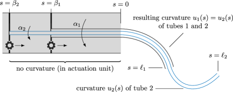
Figure 1: Example of two concentric tubes with pre-curvature $\mathbf{u}_{i}^{\star}$ extended by $\beta_{i}$ and rotated by $\alpha_{i}$, $i=1,2$ inside the actuation unit. This results in a path $\mathbf{p}(s)$ with curvature $\mathbf{u}(s)$, $s\in[\bar{\beta},\bar{\ell}]$ denoting arc length. The tubes are straight for $s\leq 0$, and coincide for $s\in[0,\ell_{1}]$. Image taken from Sauerteig et al. (2022).

Each tube by itself (that is, not yet inserted into any other tube) traces out a curve in $\mathbb{R}^{3}$, denoted $\mathbf{p}_{i}^{\star}(s)\in\mathbb{R}^{3}$. Attached to each tube is a right-handed coordinate frame, continuous with respect to arc-length, with the $z$-axis tangent to the curve’s velocity vector. Thus, each tube has an associated homogeneous transformation, $g_{i}^{\star}(s)\in\mathrm{SE(3)}$,

$$g_{i}^{\star}(s)=\left[\begin{array}[]{cc}\mathbf{R}_{i}^{\star}(s)&\mathbf{p}_{i}^{\star}(s)\\ \mathbf{0}_{3}^{\top}&1\end{array}\right],\quad i=1,2,\dots,n,$$

$s\in[\beta_{i},\ell_{i}]$. Each tube’s pre-curvature as a function of arc-length is specified by $\mathbf{u}_{i}^{\star}(s)=(\mathbf{u}_{ixy}^{\star}(s),u_{iz}^{\star}(s))^{\top}\in\mathbb{R}^{3}$, $\mathbf{u}_{ixy}^{\star}(s)=(u_{ix}^{\star}(s),u_{iy}^{\star}(s))^{\top}\in\mathbb{R}^{2}$ and satisfies,

$$\mathbf{u}_{i}^{\star}(s)=\left((\mathbf{R}_{i}^{\star}(s))^{\top}\dot{\mathbf{R}}_{i}^{\star}(s)\right)^{\vee}\in\mathbb{R}^{3}.$$

Furthermore, each tube’s cross-section is an annulus with constant inner and outer diameter, $\rho_{i}^{\mathrm{i}}$ and $\rho_{i}^{\mathrm{o}}$, respectively; $I_{i}$ denotes its second moment of area (which is constant) about the $x$ or $y$ axis; $E_{i}$ denotes its Young’s modulus; $G_{i}$ denotes its shear modulus; and $J_{i}=2I_{i}$ denotes its polar moment.

When the tubes are inserted into one another they interact and deform, tracing out a curve with position $\mathbf{p}_{i}(s)$ and rotation $\mathbf{R}_{i}(s)$. Let this transformation be denoted,

$$g_{i}(s)=\left[\begin{array}[]{cc}\mathbf{R}_{i}(s)&\mathbf{p}_{i}(s)\\ \mathbf{0}_{3}^{\top}&1\end{array}\right],\quad i=1,2,\dots,n.$$

It is assumed that an outer tube does not extend beyond any of its inner tubes. The effects of various phenomena, such as friction, hysteresis, etc. are ignored, see Rucker (2011) for full assumption details.

Where the tubes overlap, their positions coincide. However, they are free to rotate about their local $z$-axes. This rotation is denoted by $\psi_{i}(s)$, which can be shown to satisfy the following differential equations, for each $i$,

$$\dot{\psi}_{i}(s) =u_{iz}(s),$$

$$\dot{u}_{iz}(s) =A_{i}\sum_{j\in T(s)}E_{j}I_{j}(\mathbf{u}_{ixy}^{\star}(s))^{\top}B_{\psi_{ij}}(s)\mathbf{u}_{jxy}^{\star}(s),$$

for $s\leq\ell_{i}$. Here, $A_{i}\coloneqq\frac{E_{i}I_{i}}{(EI)(s)G_{i}J_{i}}$, $(EI)(s)\coloneqq\sum_{i\in T(s)}E_{i}I_{i}$ and $T(s)\coloneqq\{i\in\{1,2,\dots,n\}:s\leq\ell_{i}\}$ denotes the tube indices of length at least $\ell_{i}$. Moreover,

$$B_{\psi_{ij}}(s)\coloneqq\left[\begin{array}[]{cc}\sin(\psi_{i}(s)-\psi_{j}(s))&-\cos(\psi_{i}(s)-\psi_{j}(s))\\ \cos(\psi_{i}(s)-\psi_{j}(s))&\sin(\psi_{i}(s)-\psi_{j}(s))\end{array}\right].$$

As with the pre-curvatures, we let $\mathbf{u}_{i}(s)=(\mathbf{u}_{ixy}(s),u_{iz}(s))=(u_{ix}(s),u_{iy}(s),u_{iz}(s))^{\top}\in\mathbb{R}^{3}$. Furthermore, the remaining components of the resulting curvature of each tube is given by the following algebraic equation,

$$\mathbf{u}_{ixy}(s)=\frac{1}{(EI)(s)}\sum_{j\in T(s)}C_{\psi_{ij}}(s)E_{j}I_{j}\mathbf{u}^{\star}_{jxy}(s),$$

where

$$C_{\psi_{ij}}(s)\coloneqq\left[\begin{array}[]{cc}\cos(\psi_{j}(s)-\psi_{j}(s))&-\sin(\psi_{j}(s)-\psi_{i}(s))\\ \sin(\psi_{j}(s)-\psi_{i}(s))&\cos(\psi_{j}(s)-\psi_{i}(s))\end{array}\right].$$

The displacement and rotation of a tube inside the actuation unit, $\beta_{i}\in\mathbb{R}_{\leq 0}$ and $\alpha_{i}\in\mathbb{R}$, respectively, produces a tortion on each tube over the section $[\beta_{i},0]$ (inside the actuation unit) resulting in,

$$\psi_{i}(0)=\alpha_{i}-\beta_{i}u_{iz}(0).$$

Furthermore, it is assumed that there is no external load on the tube, and thus,

$$u_{iz}(\ell_{i})=0.$$

Recall the assumption that each tube’s local $z$-axis points in the direction of the curve’s velocity vector. Thus, also taking the relation $\mathbf{u}_{i}(s)=\left((\mathbf{R}_{i}(s))^{\top}\dot{\mathbf{R}}_{i}(s)\right)^{\vee}$ into account, we identify the twist coordinates, $\xi_{i}(s)=(\boldsymbol{e}_{3}^{\top},\mathbf{u}_{i}(s)^{\top})$, $\boldsymbol{e}_{3}\coloneqq(0,0,1)^{\top}$. The matrix $g^{-1}(s)\dot{g}(s)=\left[\begin{array}[]{cc}\mathbf{R}^{\top}(s)\dot{\mathbf{R}}(s)&\mathbf{R}^{\top}(s)\dot{\mathbf{p}}(t)\\ \mathbf{0}_{3}^{\top}&0,\end{array}\right]\in\mathfrak{se}(3)$ is a twist. Thus, we obtain, for each $i\in\{1,2\dots,n\}$,

$$\dot{\mathbf{R}}_{i}(s) =\mathbf{R}_{i}(s)\hat{\mathbf{u}}_{i}(s),$$

$$\dot{\mathbf{p}}_{i}(s) =\mathbf{R}_{i}(s)\boldsymbol{e}_{3},$$

for all $s\in[\beta_{i},\ell_{i}]$.

2.2 The Path Planning Problem

Recall that all the tubes’ positions coincide and that no tube extends beyond any of its inner tubes. Thus, it suffices to only consider the evolution of $\mathbf{p}_{n}$. Our goal is to choose, for $i=1,2,\dots,n$, the precurvatures, $\mathbf{u}_{i}^{\star}$ (which we assume constant for all $s\in[\beta_{i},\ell_{i}]$); the tube lengths, $L_{i}$; the tube inner and outer diameters, $\rho_{i}^{\mathrm{i}}$ and $\rho_{i}^{\mathrm{o}}$; the actuator parameters, $(\alpha_{i},\beta_{i})$; the initial position of the inner-most tube on the skull, $\mathbf{p}_{n}^{0}$; and its initial orientation $\mathbf{R}_{n}^{0}$, such that the resulting curve traced out by the inner tube reaches a target area while avoiding a number of obstacles enclosing sensitive brain areas. The tube is also not allowed to cross from one brain hemisphere to the other.

Let $\mathbf{u}^{\star}\coloneqq(\mathbf{u}^{\star\top}_{1},\mathbf{u}^{\star\top}_{2},\dots,\mathbf{u}^{\star\top}_{n})^{\top}\in\mathbb{R}^{3n}$, $(\boldsymbol{\rho}^{\mathrm{i}},\boldsymbol{\rho}^{\mathrm{o}}):=({\rho}^{\mathrm{i}}_{1},{\rho}^{\mathrm{i}}_{2},\dots,{\rho}^{\mathrm{i}}_{n},{\rho}^{\mathrm{o}}_{1},{\rho}^{\mathrm{o}}_{2},\dots,{\rho}^{\mathrm{o}}_{n})^{\top}\in\mathbb{R}^{2n}$, $(\boldsymbol{\alpha}^{\top},\boldsymbol{\beta}^{\top})^{\top}\coloneqq(\alpha_{1},\alpha_{2},\dots,\alpha_{n},\beta_{1},\beta_{2},\dots,\beta_{n})^{\top}\in\mathbb{R}^{2n}$, $\mathbf{L}\coloneqq(L_{1},L_{2},\dots,L_{n})^{\top}\in\mathbb{R}^{n}$, and let the decision space be denoted by,

$$\mathbb{D}\coloneqq\{(\mathbf{u}^{\star},\mathbf{L},\boldsymbol{\rho}^{\mathrm{i}},\boldsymbol{\rho}^{\mathrm{o}},\boldsymbol{\alpha},\boldsymbol{\beta},\mathbf{p}_{n}^{0},\mathbf{R}_{n}^{0})\in\mathbb{R}^{8n+3}\times\mathrm{SO(3)}\}.$$

Our path planning problem (PPP) may be expressed as follows,

$$(\mathrm{PPP}) \quad\quad\quad\quad\min_{\mathbf{d}\in\mathbb{D}}\quad J(\mathbf{d})$$

$$\mathrm{s.t.}\quad \mathrm{For\ all\ }s\in[0,\ell_{n}]\mathrm{\ and\ all\ }i\in\{1,2,\dots,n\}:$$

$$\mathbf{p}_{n}(s)\in(\mathcal{S}\cap\mathcal{H})\setminus\mathcal{E}.$$

$$\dot{\mathbf{p}}_{n}(s)=\mathbf{R}_{n}(s)\mathbf{e}_{3},$$ (1)

$$\dot{\mathbf{R}}_{n}(s)=\mathbf{R}_{n}(s)\hat{\mathbf{u}}_{n}(s),$$ (2)

$$\dot{\psi}_{i}(s)=u_{iz}(s),$$ (3)

$$\dot{u}_{iz}(s)=A_{i}\sum_{j\in T(s)}E_{j}I_{j}(\mathbf{u}_{ixy}^{\star})^{\top}B_{\psi_{ij}}(s)\mathbf{u}_{jxy}^{\star},$$ (4)

$$\mathbf{u}_{ixy}(s)=\frac{1}{(EI)(s)}\sum_{j\in T(s)}C_{\psi_{ij}}(s)E_{j}I_{j}\mathbf{u}^{\star}_{jxy}.$$ (5)

$$\mathbf{p}_{n}(0)=\mathbf{p}_{n}^{0}\in\partial\mathcal{S},$$ (6)

$$\mathbf{R}_{n}(0)=\mathbf{R}_{n}^{0}\in\mathrm{SO(3)},$$ (7)

$$\mathbf{p}_{n}(\ell_{n})\in\mathbb{P}_{f},$$ (8)

$$0<L_{1}\leq L_{2}\leq\dots\leq L_{n}.$$ (9)

$$u_{iz}(\ell_{i})=0,$$ (10)

$$\psi_{i}(0)=\alpha_{i}-\beta_{i}u_{iz}(0),$$ (11)

$$\ell_{i}=L_{i}+\beta_{i},$$ (12)

$$0\leq\alpha_{i}<2\pi,$$ (13)

$$-L_{i}\leq\beta_{i}\leq 0.$$ (14)

The cost function is chosen to minimise arc length, thus, $J:\mathbb{D}\rightarrow\mathbb{R}_{\geq 0}$ is given by,

$$J(\mathbf{d})\coloneqq\ell_{n}.$$

The skull and brain are modelled by an ellipsoid, $\mathcal{S}=\mathrm{Ell}(\boldsymbol{c}^{\mathcal{S}},Q^{\mathcal{S}})$; $\mathbb{P}_{f}\subset\mathbb{R}^{3}$ indicates the target set; $\mathcal{H}$ is a half space containing the brain hemisphere wherein the target set lies; and $\mathcal{E}\coloneqq\bigcup_{j\in\mathbb{I}^{K}}\mathcal{E}_{j}$, with $\mathcal{E}_{j}=\mathrm{Ell}(\mathbf{c}^{\mathcal{E}_{j}},Q^{\mathcal{E}_{j}})$, and $K\in\mathbb{N}$, denotes the ellipsoidal obstacles. If a solution to the problem exists, we denote it by $\bar{\mathbf{d}}\in \mathbb{D}$.

3 Obtaining the Constraints from Labelled Data

This section describes how we construct the various constraints appearing in (PPP) from labelled data, which we assume to be point clouds (voxel centres) in $\mathbb{R}^{3}$ that indicate relevant areas of a patient’s brain. These are points that define the skull, $\mathbb{V}^{\mathcal{S}}=\left\{\boldsymbol{v}^{\mathcal{S}}_{i}\right\}_{i\in\mathbb{I}^{n_{\mathrm{s}}}}$; the target area, $\mathbb{V}^{\mathrm{t}}=\left\{\boldsymbol{v}^{\mathrm{t}}_{i}\right\}_{i\in\mathbb{I}^{n_{\mathrm{t}}}}$; $K\in\mathbb{N}$ obstacles, $\mathbb{V}^{\mathrm{o}}_{j}=\left\{\boldsymbol{v}^{\mathrm{o}}_{ij}\right\}_{i\in\mathbb{I}^{n­_{\mathrm{oj}}}}$, $j=1,2,\dots,K$; and points on a plane that divide the brain into its hemispheres, $\mathbb{V}^{\mathrm{h}}=\left\{\boldsymbol{v}^{\mathrm{h}}_{i}\right\}_{i\in\mathbb{I}^{n_{\mathrm{h}}}}$.

3.1 Fitting the hyperplane

The plane dividing the hemispheres, which we label $\Pi:=\{\mathbf{x}\in\mathbb{R}^{3}:\mathbf{x}^{\top}\boldsymbol{h}=1\}$, $\boldsymbol{h}\in\mathbb{R}^{3}$, is found by solving for $\boldsymbol{h}$ in the system of equations,

$$(\boldsymbol{v}^{\mathrm{h}}_{i})^{\top}\boldsymbol{h}=1,\quad i\in\mathbb{I}^{n_{\mathrm{h}}},$$

via least-squares linear regression. If all the target points $\mathbb{V}^{\mathrm{t}}$ are contained in one half space defined by this plane, then we take $\mathcal{H}$ to be this half space. Otherwise, if target points appear in both hemispheres, we solve (PPP) twice: once with $\mathcal{H}=\{\mathbf{x}:\mathbf{x}^{\top}\boldsymbol{h}\leq 0\}$, and once with $\mathcal{H}=\{\mathbf{x}:\mathbf{x}^{\top}\boldsymbol{h}\geq 0\}$ and choose the best solution of the two problems.

3.2 Fitting the skull

The ellipsoid containing the brain and the skull, $\mathcal{S}=\mathrm{Ell}(\boldsymbol{c}^{\mathcal{S}},Q^{\mathcal{S}})$, is found as a best-fit ellipsoid for all the points in $\mathbb{V}^{\mathcal{S}}\cap\mathcal{H}$ by solving,

$$\min_{\boldsymbol{c}^{\mathcal{S}},Q^{\mathcal{S}}}\quad \sum_{i\in\mathbb{I}^{n_{\mathrm{s}}}_{\mathrm{new}}}\left(\|\boldsymbol{v}^{\mathcal{S}}_{i}-\boldsymbol{c}^{\mathcal{S}}\|_{Q^{\mathcal{S}}}^{2}-1\right)^{2}$$

s.t. $$Q^{\mathcal{S}}\succ 0,$$

$$\boldsymbol{c}^{\mathcal{S}}\in\mathbb{R}^{3},$$

where $\mathbb{I}^{n_{\mathrm{s}}}_{\mathrm{new}}:=\left\{i\in\mathbb{I}^{n_{\mathrm{s}}}:\boldsymbol{v}^{\mathcal{S}}_{i}\in(\mathbb{V}^{\mathcal{S}}\cap\mathcal{H})\right\}$.

By using fewer points in the fitting as we have done here we obtain faster execution times without loss of accuracy. Positive definiteness for a matrix $Q$ can be achieved in the following two ways. One is the Cholesky decomposition, $Q=GG^{\top}$, with $G\in\mathbb{R}^{3\times 3}$ a lower triangular matrix and the main diagonal entries greater than 0. The second, and in our experiments more stable one, is with rotation matrices, $Q=R^{\top}MR$, with $M\in\mathbb{R}^{3\times 3}$, a diagonal matrix with positive entries on the main diagonal, and $R\in\mathrm{SO(3)}$, described by quaternions. This formulation allows for setting constraints of the eigenvalues of $Q$ easily.

3.3 Fitting the target

The target area is modelled as an ellipsoid enclosed by the target points, so that it lies completely inside the point cloud of the target. The target’s most exterior points, forming the boundary $\partial\mathbb{V}^{\mathrm{t}}$ of the point cloud can be for example found with MATLAB’s boundary-function. A tight boundary (meaning not just the convex hull) is preferred, so that no part of the ellipsoid reaches outside of the point cloud. Let $\delta_{\mathrm{MRI}}$ denote the minimal distance between any two points of $\mathbb{V}^{\mathrm{t}}$. If one of the ellipsoid’s semi-axes was shorter than $\delta_{\mathrm{MRI}}$, it could lie between all the target points and thus exit the point cloud, so the eigenvalues of $Q^{\mathrm{t}}$ are constrained to prevent this, resulting in the optimization problem,

$$\min_{\boldsymbol{c}^{\mathrm{t}},Q^{\mathrm{t}}}\quad \sum_{i\in\mathbb{I}^{n_{\mathrm{t}}}_{\mathrm{new}}}\|\boldsymbol{v}^{\mathrm{t}}_{i}-\boldsymbol{c}^{\mathrm{t}}\|_{Q^{\mathrm{t}}}^{2}$$

s.t. $$\operatorname*{eig}(Q^{\mathrm{t}})>\left(\frac{2}{\delta_{\mathrm{MRI}}}\right)^{2}$$

$$\|\boldsymbol{v}^{\mathrm{t}}_{i}-\boldsymbol{c}^{\mathrm{t}}\|_{Q^{\mathrm{t}}}^{2}\geq 1\quad\forall\ i\in\mathbb{I}^{n_{\mathrm{t}}}_{\mathrm{new}},$$

where $\mathbb{I}^{n_{\mathrm{t}}}_{\mathrm{new}}:=\{i\in\mathbb{I}^{\mathrm{t}}:\boldsymbol{v}^{\mathrm{t}}_{i}\in\partial\mathbb{V}^{\mathrm{t}}\}$, so that,

$$\mathbb{P}_{f}=\left\{\boldsymbol{x}:\|\boldsymbol{x}-\boldsymbol{c}^{\mathrm{t}}\|_{Q^{\mathrm{t}}}^{2}\leq 1\right\}.$$

The minimisation of the target points’ $Q^{\mathrm{t}}$-distance is equivalent to maximising the ellipsoid’s volume, the product of the eigenvalues of $M$, but with faster convergence and more consistent results.

3.4 Fitting the obstacles

The same trick from the previous subsection is used in the formulation of enclosing ellipsoids for the obstacles. For an obstacle set $\mathbb{V}^{\mathrm{o}}_{j}$ we solve,

$$\min_{\boldsymbol{c}^{\mathrm{o}}_{j},Q^{\mathrm{o}}_{j}}\quad -\sum_{i\in\mathbb{I}^{n­_{\mathrm{oj}}}_{\mathrm{new}}:}\|\boldsymbol{v}^{\mathrm{o}}_{ij}-\boldsymbol{c}^{\mathrm{o}}_{j}\|_{Q^{\mathrm{o}}_{j}}^{2}$$

s.t. $$Q^{\mathrm{o}}_{j}\succ 0$$

$$\|\boldsymbol{v}^{\mathrm{o}}_{ij}-\boldsymbol{c}^{\mathrm{o}}_{j}\|_{Q^{\mathrm{o}}_{j}}^{2}\leq 1\quad\forall\ i\in\mathbb{I}^{n­_{\mathrm{oj}}}_{\mathrm{new}}$$ (15)

where $\mathbb{I}^{n­_{\mathrm{oj}}}_{\mathrm{new}}:=\{i\in\mathbb{I}^{n­_{\mathrm{oj}}}:\boldsymbol{v}^{\mathrm{o}}_{ij}\in\mathbb{V}^{\mathrm{o}}_{j}\cap\mathcal{H}\}$. This provides the enclosing ellipsoids, $\mathcal{E}_{j}=\left\{\boldsymbol{x}:\|\boldsymbol{x}-\boldsymbol{c}^{\mathrm{o}}_{j}\|_{Q^{\mathrm{o}}_{j}}^{2}\geq 1\right\}$.

3.5 Division of obstacle points

When building the obstacle ellipsoids, we are interested in fully covering all of the obstacle points, given by the construction of enclosing ellipsoids, but also not include large volumes of non-obstacle regions. One major contributor to this problem is if non-connected areas are captured by the same ellipsoid, as it might happen with the k-means algorithm, shown by Hackenberg et al. (2021). Applying DBSCAN, a density-based clustering algorithm by Ester et al. (1996), beforehand can alleviate this flaw. The distance $\delta_{\mathrm{MRI}}$ is used as the search radius for DBSCAN. To evaluate how well the ellipsoids cover the obstacle points and the surrounding area, the coverage is calculated as the number of obstacle points divided by the number of grid points on the MRI grid inside the cluster. Algorithm 1 shows the pseudo-code describing the steps.

Algorithm 1 Clustering of obstacle points

1:obstacle points $\boldsymbol{v}^{\mathrm{o}}$ and threshold $c_{\mathrm{th}}$

2:Cluster $\boldsymbol{v}^{\mathrm{o}}$ using DBSCAN to get $\boldsymbol{v}^{\mathrm{o}}_{i}$.

3:for each $i$ do

4:     while true do

5:         Cluster $\boldsymbol{v}^{\mathrm{o}}_{i}$ with k-means to get $\boldsymbol{v}^{\mathrm{o}}_{ij}$.

6:         for each $j$ do

7:              Solve (3.4) with $\boldsymbol{v}^{\mathrm{o}}_{ij}$.

8:         end for

9:         if $\frac{\text{\# MRI grid points in ellipsoids}}{\text{\# obstacle points in ellipsoid}}\leq c_{\mathrm{th}}$ then

10:              Increase the number of clusters for k-means.

11:         else

12:              Exit the while loop.

13:         end if

14:     end while

15:     Add the $j$ ellipsoids to the obstacle set.

16:end for

3.6 Numerical results

Figures 4-4 show the optimisation results for the three different types of ellipsoids. In Fig. 4, only the skull points in the admissible half-space are displayed. It shows that an ellipsoid is a good approximation for the skull. As already mentioned before, the ellipsoid in Fig. 4 covers a larger volume than the voxels marked as obstacles. This can be seen as there are parts in the ellipsoid without obstacle points. The target modelling is successful as well, still the ellipsoid underestimates the size of the target region. Overall, this problem has 1179 obstacle ellipsoids resulting in a convoluted obstacle field, partly shown in Fig. 6.

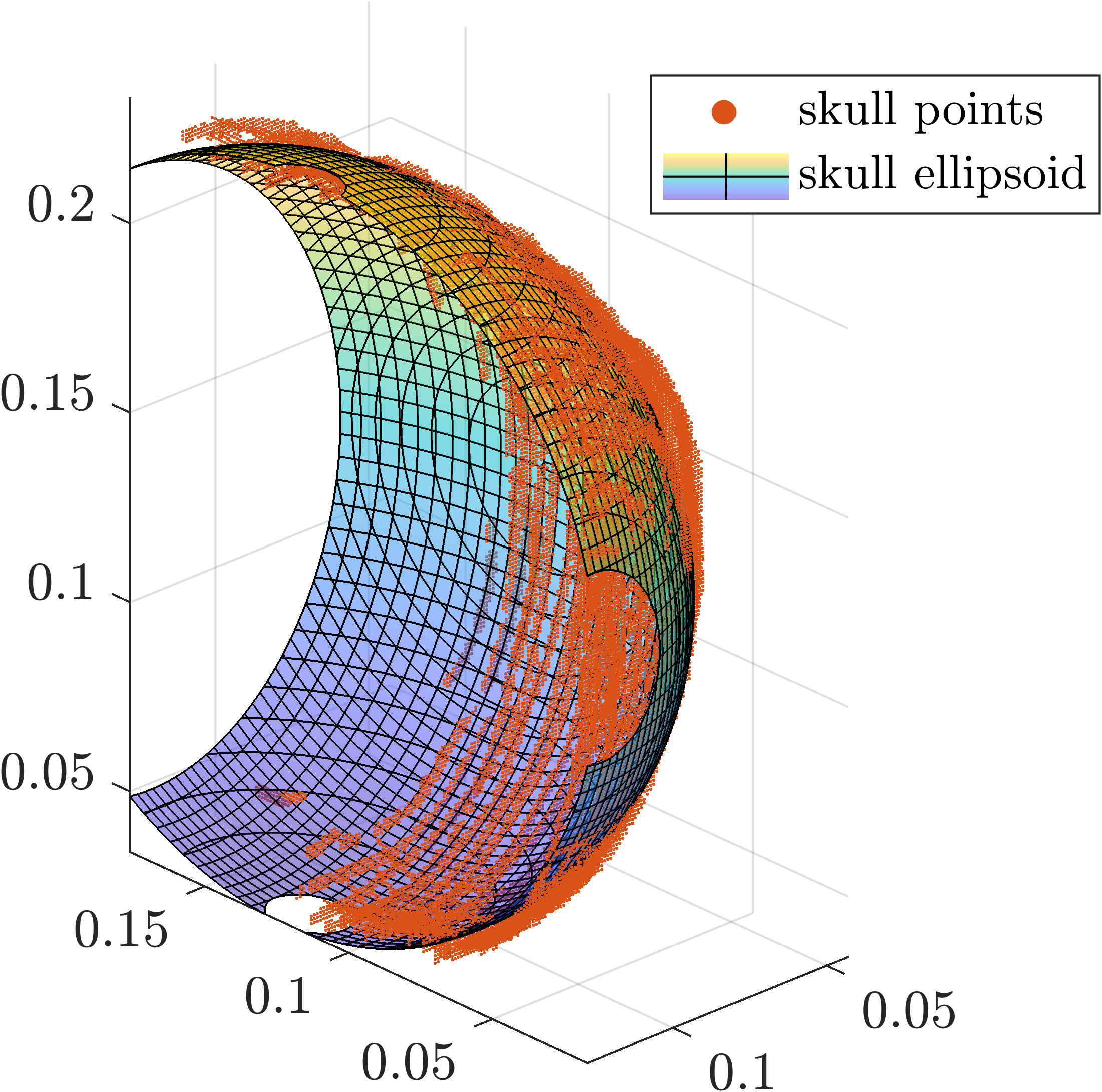
Figure 2: A best-fit ellipsoid is used to model the skull around the allowed hemisphere. An ellipsoid seems to be a good approximation for the skull.

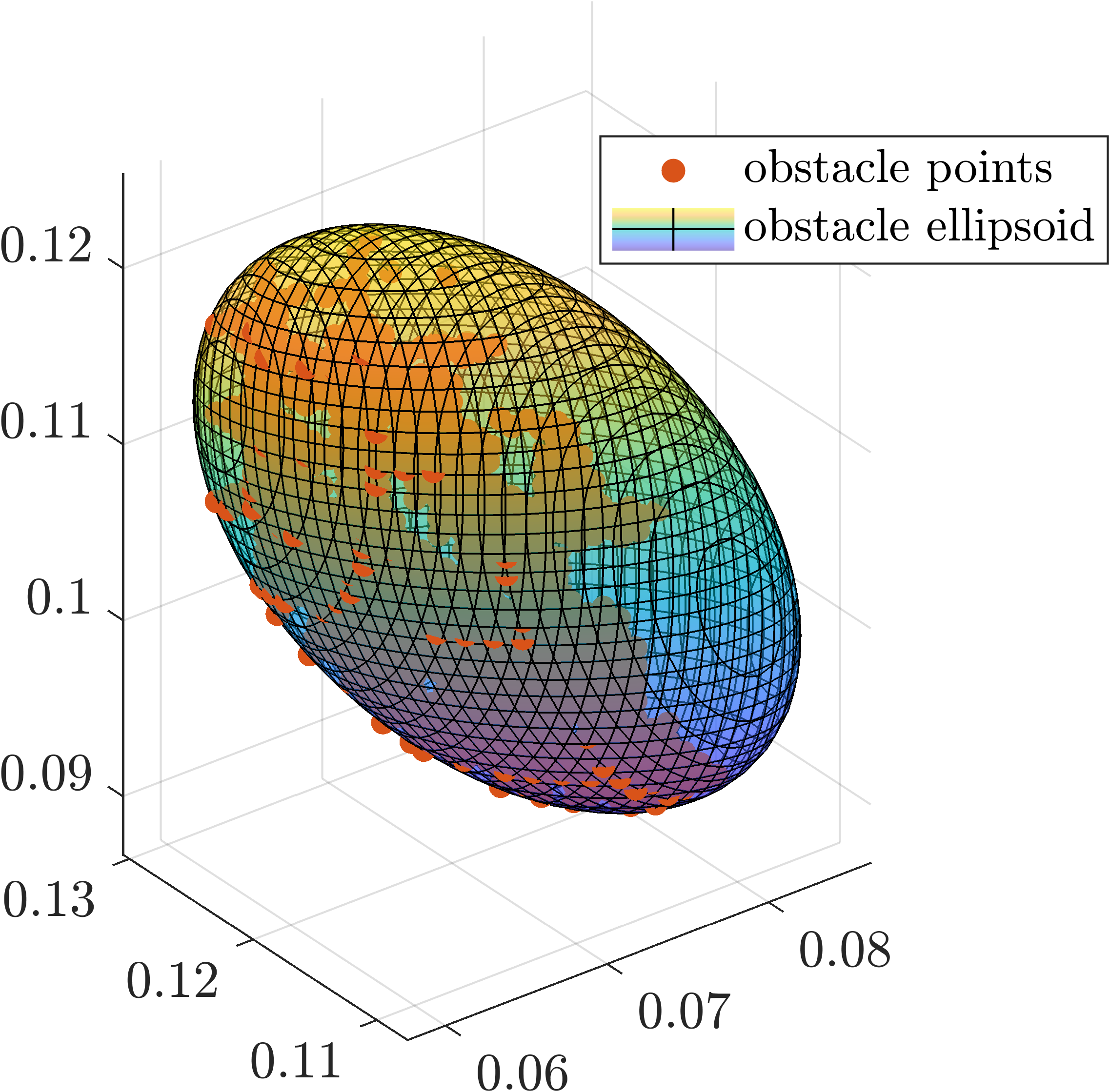
Figure 3: Enclosing ellipsoid as an approximation for the obstacles. Parts of the ellipsoid contain no obstacle points, where the ellipsoid is disallowing non-critical parts of the brain.

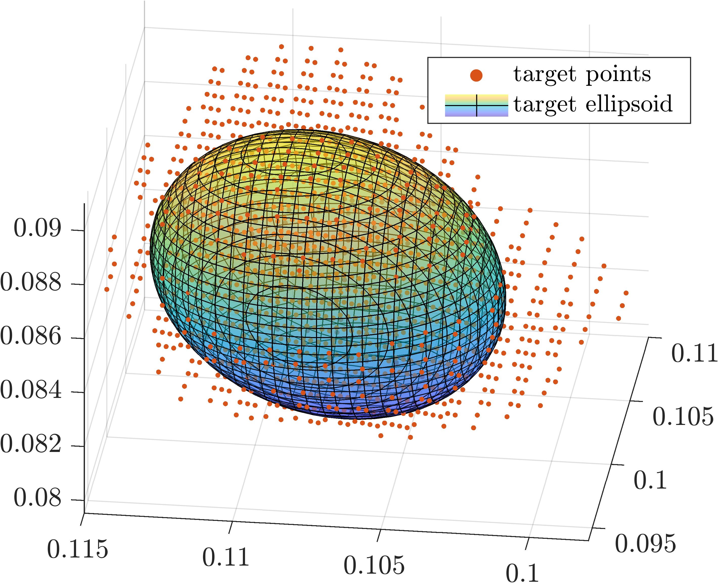
Figure 4: The target volume is modelled as an ellipsoid enclosed by the point cloud. The ellispoid is an underestimation to ensure that the cannula enters the target.

4 Solution Approach via Homotopy

The path planning problem we consider is nonlinear and highly nonconvex. With realistic data (where hundreds of ellipsoids may be present) numerical solvers often do not converge and even if they do, need very long execution times. Thus, using similar ideas from Bergman and Axehill (2018) and De Marinis et al. (2022), we introduce a homotopy on some of the obstacles’ positions, where at the one extreme they are removed from the skull’s interior, and at the other they are located at their original position. We then iteratively solve relaxed problems, using the solution with a current parameter as the initial guess for the solution with the next parameter (see Algorithm 2).

For a given homotopy parameter $\lambda\in[0,1]$ the relaxed problem reads,

$$(\mathrm{PPP}^{\lambda}) \quad\quad\quad\quad\min_{\mathbf{d}\in\mathbb{D}}\quad J(\mathbf{d})$$

$$\mathrm{s.t.}\quad \mathrm{For\ all\ }s\in[0,\ell_{n}]\mathrm{\ and\ all\ }i\in\{1,2,\dots,n\}:$$

$$\mathbf{p}_{n}(s)\in(\mathcal{S}\cap\mathcal{H})\setminus\mathcal{E}^{\mathrm{fix}},$$

$$\mathbf{p}_{n}(s)\in(\mathcal{S}\cap\mathcal{H})\setminus\mathcal{E}^{\lambda},$$

$$\eqref{PPP_eq_1}-\eqref{PPP_eq_2}.$$

Here we let

$$\mathcal{E}^{\mathrm{fix}}=\bigcup_{j\in\mathbb{I}^{\mathrm{fix}}}\mathcal{E}_{j},$$

where $\mathbb{I}^{\mathrm{fix}}\subseteq\mathbb{I}^{K}$ is the index set of ellipsoids we do not want to perturb with $\lambda$; and

$$\mathcal{E}^{\lambda}=\bigcup_{j\in\mathbb{I}\setminus\mathbb{I}^{\mathrm{fix}}}\mathcal{E}_{j}^{\lambda},$$

where

$$\mathcal{E}_{j}^{\lambda}=\mathrm{Ell}([1-\lambda]\mathbf{c}_{j}^{\mathrm{init}}+\lambda\mathbf{c}_{j}^{\mathrm{o}}),Q^{\mathrm{o}}_{j}),$$

indicates the ellipsoids that we want to perturb. Again, if a solutions exists, we denote it by $\bar{\mathbf{d}}^{\lambda}$. Thus, $\lambda$ moves the chosen ellipsoids along the line segment that connects their original positions, $\mathbf{c}_{j}^{\mathrm{o}}$, with arbitrary user-specified positions, $\mathbf{c}_{j}^{\mathrm{init}}$, where the entire ellipsoid $\mathcal{E}_{j}$ is located outside the skull. The homotopy algorithm we employ is presented in Algorithm 2.

Algorithm 2 Homotopy Algorithm

1:initial guess $\mathbf{d}^{0}$; step size $\Delta>0$

2:$\lambda\leftarrow 0$

3:$\mathbf{d}\leftarrow\mathbf{d}^{0}$

4:while $\lambda<1$ do

5:     try solve $\mathrm{PPP}^{\lambda}$ with $\mathbf{d}$ as initial guess.

6:     if solution to $\mathrm{PPP}^{\lambda}$ is found then

7:         $\mathbf{d}\leftarrow\bar{\mathbf{d}}^{\lambda}$

8:         $\lambda\leftarrow\min\{1,\lambda+\Delta\}$

9:     else

10:         break while loop

11:     end if

12:end while

13:return $\mathbf{d}$, $\lambda$

4.1 Heuristic for calculating user-specified positions $\mathbf{c}_{j}^{\mathrm{init}}$

The problem of finding a feasible cannula configuration is simpler if there are just a few obstacles. With an increasing number, the problem becomes so hard that the solver does not converge. As our aim is to shift the obstacles out of the way, one idea is to take an initial guess with very few obstacles for $\mathcal{E}^{\mathrm{fix}}$ (so few that the problem is easily solvable) and solve the problem to get an initial tube configuration. We then let $\mathbf{p}^{a}=\mathbf{p}(0)$ and $\mathbf{p}^{b}=\mathbf{p}(\ell_{n})$. All the non-fixed obstacles are shifted orthogonally from the line segment connecting $\mathbf{p}^{a}$ and $\mathbf{p}^{b}$. The factor

$$a_{i}=\frac{(\boldsymbol{c}^{\mathrm{o}}_{i}-\mathbf{p}^{a})^{\top}(\mathbf{p}^{b}-\mathbf{p}^{a})}{\|(\mathbf{p}^{b}-\mathbf{p}^{a})\|_{2}^{2}}$$

is needed to find the point closest on the line segment

$$\boldsymbol{l}_{i}=\left\{\begin{matrix}\mathbf{p}^{a},&\text{if }a_{i}<0\\ \mathbf{p}^{a}+a_{i}(\mathbf{p}^{b}-\mathbf{p}^{a}),&\quad\ \ \,\text{if }0\leq a_{i}\leq 1\\ \mathbf{p}^{b},&\text{if }a_{i}>1\end{matrix}\right..$$

Thus, the user-specified positions

$$\mathbf{c}_{i}^{\mathrm{init}}=\boldsymbol{c}^{\mathrm{o}}_{i}+0.4\frac{\boldsymbol{c}^{\mathrm{o}}_{i}-\boldsymbol{l}_{i}}{\|\boldsymbol{c}^{\mathrm{o}}_{i}-\boldsymbol{l}_{i}\|_{2}},\ \forall\ i\in(\mathbb{I}\setminus\mathbb{I}^{\mathrm{fix}})$$

are shifted to a distance of $400\text{\,}\mathrm{mm}$ from the line segment, which is typically outside of the skull. Fig. 5 shows the approach on an example.

Figure 5: The obstacle centres are pushed away perpendicular to the line segment connecting the entry and terminal point of the initial guess.

4.2 Numerical results

Next, we display the numerical results of using the homotopy algorithm on a case study. CasADi by Andersson et al. (2019) is used to formulate the optimisation problem, while $(\mathrm{PPP}^{\lambda})$ is solved with IPOPT by Wächter and Biegler (2006). Even though interior-point methods are known to be hard to warm-start (see for example John and Yıldırım (2008)), we show that they work well in this problem. The following table contains the values of the IPOPT parameters we changed.

warm_start_init_point	yes
mu_init	1e-8
warm_start_mult_bound_push	1e-10
warm_start_slack_bound_push	1e-10
warm_start_bound_push	1e-8
warm_start_bound_frac	1e-8
warm_start_slack_bound_frac	1e-10

The given case-study is intended to be solved using three tubes, with $u_{y,i}^{\star}=0$, $L_{i}=$600\text{\,}\mathrm{mm}$\ \forall\ i\in[1,3]$, and a maximal outer diameter of the outer-most tube of $\rho^{\mathrm{o}}_{1}=$8\text{\,}\mathrm{mm}$$. The length of the inner tube is minimised over the tube actuations $\boldsymbol{\alpha}$ and $\boldsymbol{\beta}$; tube lengths, $\mathbf{L}$; the tube curvatures $u_{i,x}^{\star}$; the inner and outer tube diameters, $\rho_{i}^{\mathrm{i}}$ and $\rho_{i}^{\mathrm{o}}$; the initial condition $\mathbf{p}_{n}^{0}$ and the initial rotaion,

$$\mathbf{R}^{0}_{n}=\begin{bmatrix}1-2(q_{2}^{2}-q_{3}^{2})&2(q_{1}q_{2}-q_{0}q_{3})&2(q_{1}q_{3}+q_{0}q_{2})\\ 2(q_{1}q_{2}+q_{0}q_{3})&1-2(q_{1}^{2}-q_{3}^{2})&2(q_{2}q_{3}-q_{0}q_{1})\\ 2(q_{1}q_{3}-q_{0}q_{2})&2(q_{2}q_{3}+q_{0}q_{1})&1-2(q_{1}^{2}-q_{2}^{2})\end{bmatrix},$$

where $\mathbf{q}^{0}_{n}=[q_{0},q_{1},q_{2},q_{3}]$ is a quaternion.

The original problem $(\mathrm{PPP})$ with its 1179 obstacles is not solvable out-of-the-box as the solver will not converge. However, a solution is found with the homotopy algorithm with $\Delta=0.1$. The following tables show the resulting values for the tube parameters and decision variables of tubes 2 and 3, as the algorithm finds that the outer most tube is not necessary, resulting in $\ell_{1}=0$.

Variable	$\ell_{2}$	$\ell_{3}$	$u_{x,2}^{\star}$	$u_{x,3}^{\star}$
Value	$13.2\text{\,}\mathrm{mm}$	$40.1\text{\,}\mathrm{mm}$	$9.99\text{\,}{\mathrm{m}}^{-1}$	$4.55\text{\,}{\mathrm{m}}^{-1}$
Variable	$\alpha_{2}$	$\alpha_{3}$	$\beta_{2}$	$\beta_{3}$
Value	1.5405	4.7425	$-0.587\text{\,}\mathrm{m}$	$-0.56\text{\,}\mathrm{m}$
Variable	$\rho^{\mathrm{i}}_{1}$	$\rho^{\mathrm{o}}_{1}$	$\rho^{\mathrm{i}}_{2}$	$\rho^{\mathrm{o}}_{2}$
Value	0.004	0.0053	0.0013	0.0026
Variable	$\mathbf{p}^{0}_{n}$
Value	$\left[0.0967,0.0769,0.0536\right]^{\top}$
Variable	$\mathbf{q}_{n}^{0}$
Value	$\left[0.6983,0.1727,-0.3151,-0.6190\right]^{\top}$

Fig. 6 shows the optimised cannula navigating through the field of the 45 closest obstacles, starting on the skull and entering the target area.

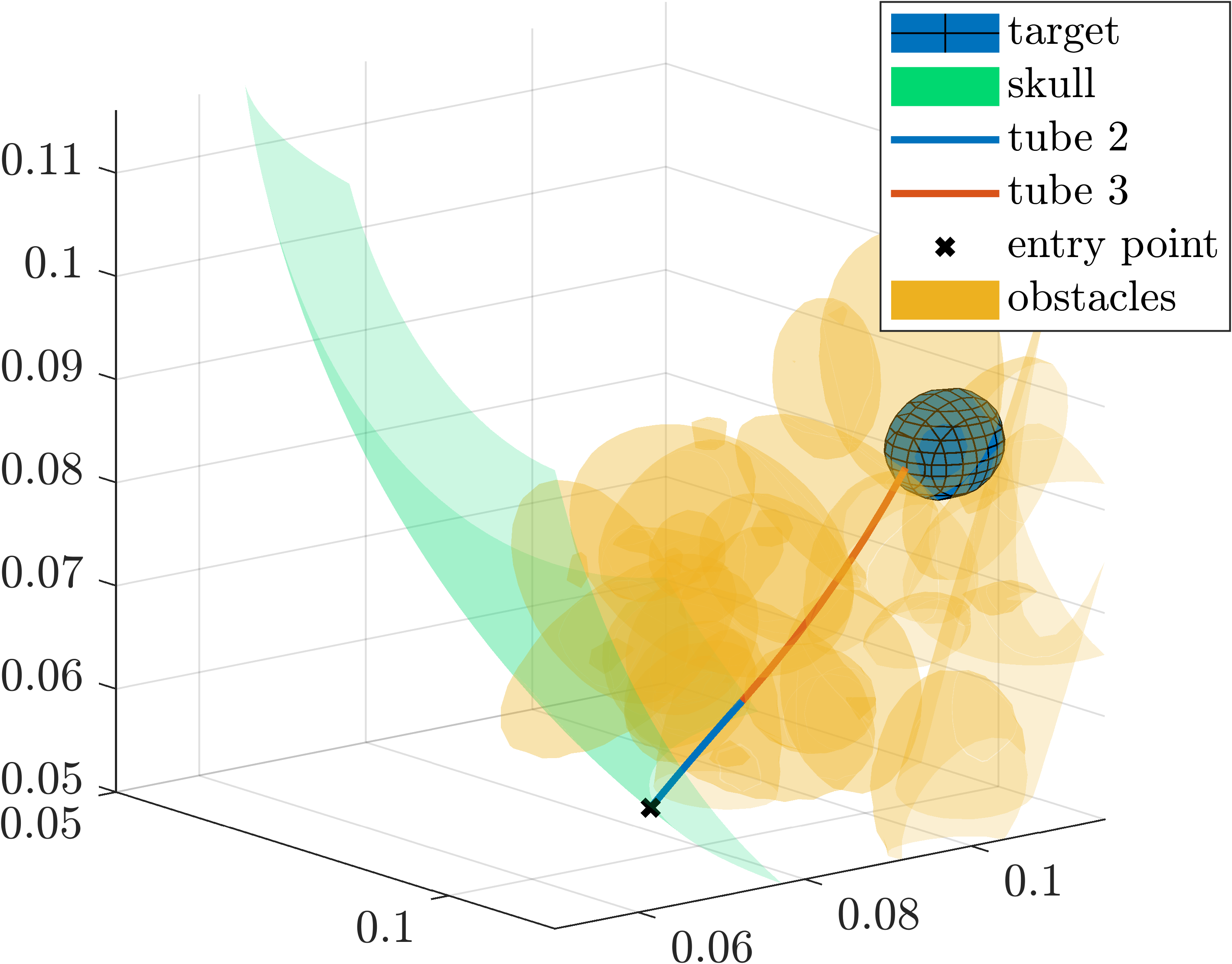
Figure 6: The solution to the given case-study reaching from the skull to the target position. The 45 ellipsoids closest to the cannula are displayed.

The same solution is displayed in Fig. 7 without the obstacles to show the resulting curvature of the cannula.

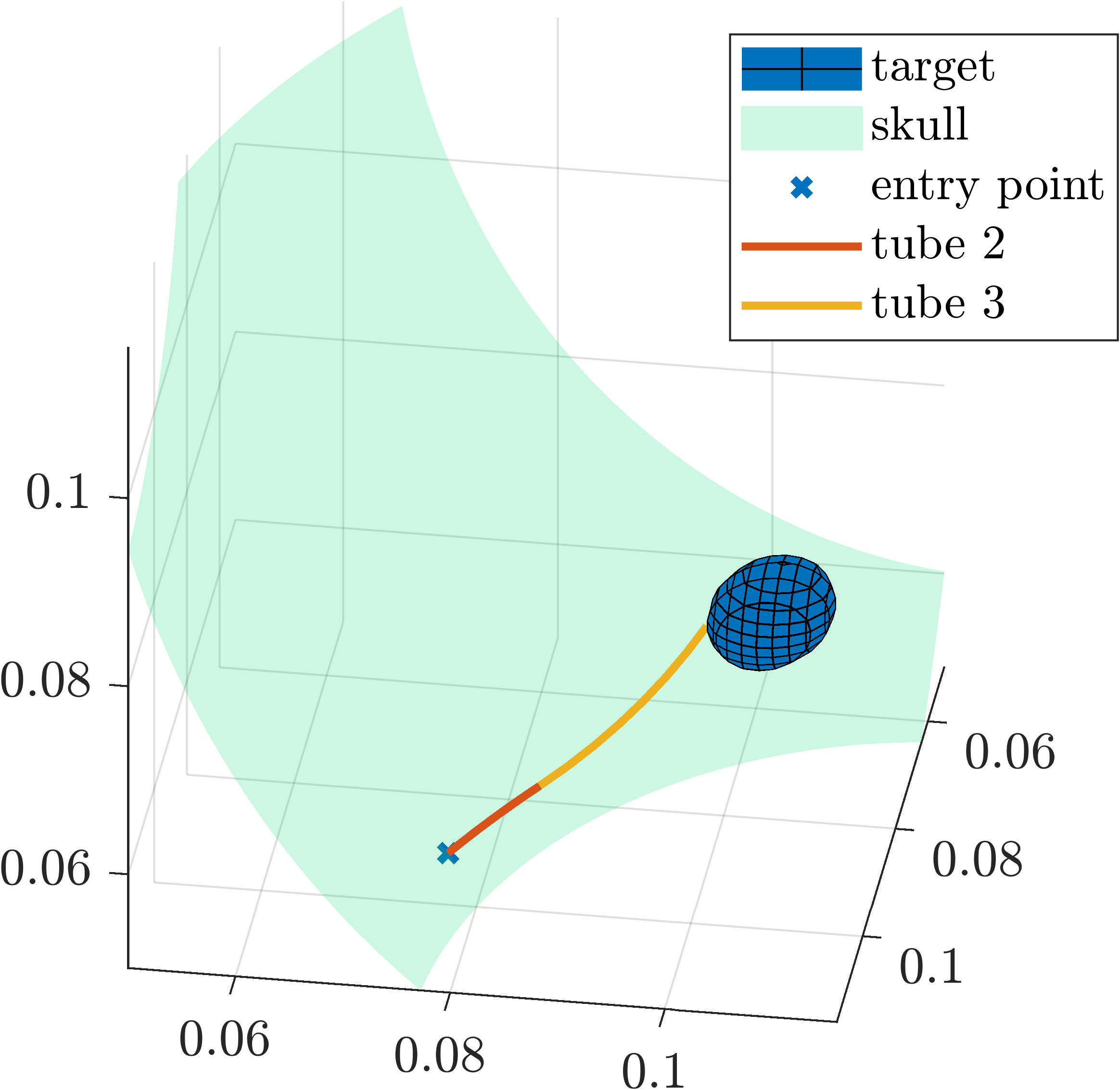
Figure 7: The solution without the obstacles.

5 Conclusion

In this work, we tackle the challenging task of optimally planning concentric tube continuum robot dimensioning and actuation in geometrically constrained spaces and present our findings in the real-world example of stereotactic neurosurgery. From labelled MRI or CT scans as a starting point, we formulate easily solvable optimisation problems for condensing the point clouds to a set of elliptical constraints. For the large number of points belonging to the obstacles, we propose an algorithm combining DBSCAN and the k-means-algorithm for separating and clustering the obstacles. By using homotopy methods, we enable the solution of the path planning problem, unsolvable out-of-the-box. The success of these methods is underlined by the application to the real-world case-study and the corresponding numerical results.

There are many areas on which future research may focus. First, the homotopy algorithm is not guaranteed to converge as $\lambda$ tends to 1 and conditions on the problem data that imply this should be investigated. Second, in moving the obstacles with the homotopy parameter we did not take care to prevent topological changes in the free space where the tubes may manoeuvre. Though we were able to find a solution to the problem we considered, these topological changes may result in discontinuities of the optimal paths from one iteration of $\lambda$ to the next, which could cause infeasibility. Third, by using the homotopy approach the final path may in fact only be locally optimal: a result of “slightly” perturbing previously-found solutions. More involved perturbations can result in global optima.

References

• Andersson et al. (2019) Andersson, J.A.E., Gillis, J., Horn, G., Rawlings, J.B., and Diehl, M. (2019). CasADi – A software framework for nonlinear optimization and optimal control. Mathematical Programming Computation, 11(1), 1–36. 10.1007/s12532-018-0139-4.
• Bergeles et al. (2015) Bergeles, C., Gosline, A.H., Vasilyev, N.V., Codd, P.J., Pedro, J., and Dupont, P.E. (2015). Concentric tube robot design and optimization based on task and anatomical constraints. IEEE Transactions on Robotics, 31(1), 67–84.
• Bergman and Axehill (2018) Bergman, K. and Axehill, D. (2018). Combining homotopy methods and numerical optimal control to solve motion planning problems. In 2018 IEEE Intelligent Vehicles Symposium (IV), 347–354. IEEE.
• Burgner et al. (2013) Burgner, J., Gilbert, H.B., and Webster, R.J. (2013). On the computational design of concentric tube robots: Incorporating volume-based objectives. In 2013 IEEE International Conference on Robotics and Automation, 1193–1198. IEEE.
• De Marinis et al. (2022) De Marinis, A., Iavernaro, F., and Mazzia, F. (2022). A minimum-time obstacle-avoidance path planning algorithm for unmanned aerial vehicles. Numerical Algorithms, 89(4), 1639–1661.
• Dhanakoti et al. (2022) Dhanakoti, S., Maddocks, J., and Weiser, M. (2022). Navigation of concentric tube continuum robots using optimal control. In Proceedings of the 19th International Conference on Informatics in Control, Automation and Robotics - ICINCO, 146–154. SciTePress.
• Dupont et al. (2009) Dupont, P.E., Lock, J., Itkowitz, B., and Butler, E. (2009). Design and control of concentric-tube robots. IEEE Transactions on Robotics, 26(2), 209–225.
• Ester et al. (1996) Ester, M., Kriegel, H.P., Sander, J., Xu, X., et al. (1996). A density-based algorithm for discovering clusters in large spatial databases with noise. In kdd, volume 96, 226–231.
• Faust (2007) Faust, R.A. (2007). Robotics in surgery: history, current and future applications. Nova Publishers.
• Flaßkamp et al. (2019) Flaßkamp, K., Worthmann, K., Mühlenhoff, J., Greiner-Petter, C., Büskens, C., Oertel, J., Keiner, D., and Sattel, T. (2019). Towards optimal control of concentric tube robots in stereotactic neurosurgery. Mathematical and Computer Modelling of Dynamical Systems, 25(6), 560–574.
• Gilbert et al. (2016) Gilbert, H.B., Rucker, D.C., and Webster III, R.J. (2016). Concentric tube robots: The state of the art and future directions. Robotics Research, 253–269.
• Granna et al. (2019) Granna, J., Nabavi, A., and Burgner-Kahrs, J. (2019). Computer-assisted planning for a concentric tube robotic system in neurosurgery. International journal of computer assisted radiology and surgery, 14(2), 335–344.
• Greiner-Petter and Sattel (2017) Greiner-Petter, C. and Sattel, T. (2017). On the influence of pseudoelastic material behaviour in planar shape-memory tubular continuum structures. Smart Materials and Structures, 26(12), 125024.
• Ha et al. (2018) Ha, J., Fagogenis, G., and Dupont, P.E. (2018). Modeling tube clearance and bounding the effect of friction in concentric tube robot kinematics. IEEE Transactions on Robotics, 35(2), 353–370.
• Hackenberg et al. (2021) Hackenberg, A., Worthmann, K., Pätz, T., Keiner, D., Oertel, J., and Flaßkamp, K. (2021). Neurosurgery planning based on automated image recognition and optimal path design. at-Automatisierungstechnik, 69(8), 708–721.
• John and Yıldırım (2008) John, E. and Yıldırım, E.A. (2008). Implementation of warm-start strategies in interior-point methods for linear programming in fixed dimension. Computational Optimization and Applications, 41(2), 151–183.
• Leibrandt et al. (2017) Leibrandt, K., Bergeles, C., and Yang, G.Z. (2017). Concentric tube robots: Rapid, stable path-planning and guidance for surgical use. IEEE Robotics & Automation Magazine, 24(2), 42–53.
• Lyons et al. (2009) Lyons, L.A., Webster, R.J., and Alterovitz, R. (2009). Motion planning for active cannulas. In 2009 IEEE/RSJ International Conference on Intelligent Robots and Systems, 801–806. IEEE.
• Murray et al. (2017) Murray, R.M., Li, Z., and Sastry, S.S. (2017). A mathematical introduction to robotic manipulation. CRC press.
• Peikert et al. (2022) Peikert, S., Kunz, C., Fischer, N., Hlaváč, M., Pala, A., Schneider, M., and Mathis-Ullrich, F. (2022). Automated linear and non-linear path planning for neurosurgical interventions. In 2022 International Conference on Robotics and Automation (ICRA), 7731–7737. IEEE.
• Rucker et al. (2010) Rucker, D.C., Jones, B.A., and Webster III, R.J. (2010). A geometrically exact model for externally loaded concentric-tube continuum robots. IEEE transactions on robotics, 26(5), 769–780.
• Rucker (2011) Rucker, D.C. (2011). The mechanics of continuum robots: model-based sensing and control. Vanderbilt University.
• Sauerteig et al. (2022) Sauerteig, P., Hoffmann, M.K., Mühlenhoff, J., Miccoli, G., Keiner, D., Urbschat, S., Oertel, J., Sattel, T., Flaßkamp, K., and Worthmann, K. (2022). Optimal path planning for stereotactic neurosurgery based on an elastostatic cannula model. IFAC-PapersOnLine, 55(20), 600–605.
• Torres and Alterovitz (2011) Torres, L.G. and Alterovitz, R. (2011). Motion planning for concentric tube robots using mechanics-based models. In 2011 IEEE/RSJ International Conference on Intelligent Robots and Systems, 5153–5159.
• Wächter and Biegler (2006) Wächter, A. and Biegler, L.T. (2006). On the implementation of an interior-point filter line-search algorithm for large-scale nonlinear programming. Mathematical programming, 106(1), 25–57.
• Webster et al. (2006) Webster, R.J., Okamura, A.M., and Cowan, N.J. (2006). Toward active cannulas: Miniature snake-like surgical robots. In 2006 IEEE/RSJ international conference on intelligent robots and systems, 2857–2863. IEEE.
• Webster et al. (2009) Webster, R.J., Swensen, J.P., Romano, J.M., and Cowan, N.J. (2009). Closed-form differential kinematics for concentric-tube continuum robots with application to visual servoing. In Experimental Robotics, 485–494. Springer.