Distance Metric Learning Loss Functions in Few-Shot Scenarios of Supervised Language Models Fine-Tuning

Abstract

This paper presents an analysis regarding an influence of the Distance Metric Learning (DML) loss functions on the supervised fine-tuning of the language models for classification tasks. We experimented with known datasets from SentEval Transfer Tasks.

Our experiments show that applying the DML loss function can increase performance on downstream classification tasks of RoBERTa-large models in few-shot scenarios. Models fine-tuned with the use of SoftTriple loss can achieve better results than models with a standard categorical cross-entropy loss function by about 2.89 percentage points from 0.04 to 13.48 percentage points depending on the training dataset. Additionally, we accomplished a comprehensive analysis with explainability techniques to assess the models’ reliability and explain their results.

Keywords natural language processing  $\cdot$ deep learning  $\cdot$ loss functions  $\cdot$ text classification  $\cdot$ explainability  $\cdot$ few-shot learning

1 Introduction

The development of new techniques in the Natural Language Processing (NLP) field has been studied over the last few years. It resulted in a few breakthroughs, which constantly stimulated waves of interest in the text processing area. The most recent discoveries are based on the Transformer architecture that enabled capturing the semantic meaning of the sentence Vaswani et al. (2017). The Transformer architecture facilitated the discovery of the BERT encoder Devlin et al. (2019) that nowadays is massively used to solve most NLP tasks by adapting it in the fine-tuning process.

Unfortunately, fine-tuning of pre-trained models has a number of flaws. First of all, it is not designed to perform well when the number of observations is limited, so large training sets are consistently required for models to perform well Bansal et al. (2019). Secondly, the fine-tuning process happens to be very unstable across different runs with different seeds, even though just a few minor components of the learning process are dependent on random seeds Zhang et al. (2020). The lack of stability is even more exacerbated in the case of few-shot learning scenarios.

On the other hand, pre-trained models are fine-tuned for a specific task using a cross-entropy objective function that focuses on learning class-specific features rather than their class representations. In other words, it only encourages inter-class distances and is not taking care of minimizing intra-class distances that would result in learning discriminative features Wen et al. (2016). This leads to a poor generalization of the model and thus causes problems with noisy or outlier data Cao et al. (2019).

However, a few research studies proposed other loss functions, i.e. Distance Metric Learning (DML) function family, which addresses the problems of the cross-entropy loss. The DML losses are meant to push representations of observations together if they belong to the same class and separate those from different classes. We believe this will be particularly helpful for few-shot learning, where the number of observations is insufficient for a suitable ordering of the embedding space. Therefore, we decided to investigate the effect of using loss functions from the DML family on fine-tuning the BERT-based encoder for downstream tasks in few-shot learning scenarios.

Our main contributions are the following:

1. We apply SoftTriple loss in the few-shot scenarios for the supervised fine-tuning language model in NLP domain.

2. We examine the effect of using loss functions from the DML family on the supervised fine-tuning of the RoBERTa-large language model.

3. We establish that SoftTriple loss is more efficient than Supervised Contrastive loss for the supervised fine-tuning RoBERTa-large language model.

4. After thorough experiments, our finding is that applying the DML loss to the RoBERTa-large language model is more viable the smaller the training set.

5. Additionally, to deeper understand the models and check their reliability we propose a comprehensive analysis and explainability techniques.

The following section is dedicated to a brief overview of the DML methods. Our new method is outlined in Section 3. The next section provides a performance analysis of the models and investigates their behaviour. Finally, a summary of the experiments is described in the last section.

2 Methodological Background

The DML loss can be applied whenever embedded representations of input observations are learned Qian et al. (2019). It is most often utilized in image processing, where the high-quality image embeddings are formed into the downstream tasks, such as k-nearest neighbours classification Weinberger and Saul (2009), clustering or image retrieval Xing et al. (2002). The main goal of DML is to minimize distances between observations from the same class while maximizing inter-class distances. Standard methods for DML is Contrastive Loss and Triplet Loss Hadsell et al. (2006); Schroff et al. (2015). In our experiments, we utilized most modern approaches such as Supervised Contrastive Learning Loss Pereyra et al. (2017) and SoftTriple Loss Qian et al. (2019).

2.1 Supervised Contrastive Learning Loss

Supervised Contrastive Learning (SupCon) is one of the modern DML approaches which outperforms traditional methods such as Triplet Loss or Contrastive Loss. The SupCon introduces temperature regularization Pereyra et al. (2017) and batch processing which means that the loss is not calculated just for a single triplet but is the average of all possible triplets from a given batch. The SupCon loss extends the self-supervised batch DML approach to the fully-supervised setting, which provides the ability to use the label information Khosla et al. (2020). Instead of contrasting one positive example for an anchor with all other observations from the batch, SupCon contrasts all examples from the same class (as positives) with all other observations from the batch as negatives. The most critical issue with this approach is that as the number of observations in the batch grows, the number of triplets grows cubically.

The SupCon loss has been previously applied in the supervised fine-tuning of the RoBERTa-large language model Gunel et al. (2020) and its formula is as follows:

where $i\in I\equiv\{1,\ldots,N\}$ denotes the index of an anchor observation $x_{i}$, $P(i)$ is the set of observations from the same class that $x_{i}$ belongs to, $A(i)\equiv I\backslash\{i\}$, $z_{i}$ denotes the representation of the $x_{i}$ observation that is outputted by the encoder. $x_{p}$ denotes observation from the same class as $x_{i}$ (positive class), while $x_{n}$ denotes the observations from different class as $i$. $\tau\in\mathcal{R}^{+}$ is a scalar temperature.

2.2 SoftTriple Loss

SoftTriple loss is another modern DML approach that extends the batch supervised DML approach. It employs proxies – artificial embeddings that are learned during the training procedure – to represent classes from the dataset. In other words, each class has its own additional set of points that best approximates the position of all observations from the class. The number of proxies is given as a hyperparameter and should reflect the global distribution of features from the class, which may have more than one focal point. The loss is calculated based on the possible triplets in the batch. It is the same as the SupCon loss. The difference is in calculating the single triplet. It is composed of the anchor (observation), positive proxy (a proxy from the anchor class) and negative proxy (a proxy from a class other than the anchor). The number of all possible triples is linear with respect to the number of original examples, while it grows cubically (as stated earlier) for the SupCon or other non-proxy losses. Therefore, this approach consumes much fewer resources and has higher performance because the proxy provides better resistance to outliers.

The following formulas define the SoftTriple loss:

$$\mathcal{S}_{i,c}^{\prime}=\sum_{k\in K}\frac{\exp\left(\frac{1}{\gamma}{E({x}_{i})}^{\top}{w}_{c}^{k}\right)}{\sum_{k\in K}\exp\left(\frac{1}{\gamma}{E({x}_{i})}^{\top}{w}_{c}^{k}\right)}{E({x}_{i})}^{\top}{w}_{c}^{k},$$ (3)

where $i\in I\equiv\{1\ldots N\}$ denotes the index of an anchor observation $x_{i}$, $y_{i}$ its corresponding label, $c\in C$ denotes the class index, $C$ denotes the class number, $k\in K$ denotes the proxy index of class $c$, $K$ denotes the number of proxies per class, $\delta$ denotes a minimum interclass margins, $\lambda$ scaling factor that reduces the outliers’ impact, $\gamma$ scaling factor for the entropy regularizer, $x_{i}$ denotes a $i$th observation’ embedding, $E(\cdot)\in\mathbf{R}^{d}$ denotes an encoder and ${w}_{c}^{k}$ are weights that represent embeddings of the class $c$.

3 Our Approach

We analyze the impact of the DML loss function on the supervised training of the pre-trained language model by extending the loss function with SupCon loss or SoftTriple loss. In general, the new loss function contains two elements; the first one is categorical cross-entropy loss applied to the output of the classification layer, and the DML loss is applied directly to the output of the encoder. The second part of our loss function maximizes distances between observations from different classes and minimizes distances between observations from the same class.

The goal function is given by the following formula:

$$\mathcal{L}=(\beta)\mathcal{\ell}_{CCE}+(1-\beta)\mathcal{\ell}_{DML},\mathcal{\ell}_{CCE}=-\frac{1}{N}\sum_{i=1}^{N}\sum_{c=1}^{C}y_{i,c}\cdot\log\hat{y}_{i,c}$$ (4)

where $N$ is the number of the observations, $C$ denotes the class number, $y_{ic}$ denotes the label of the class $c$ for the $i$th observation, $p_{ic}$ denotes the models’s predicted probability of the $i$th observation for the $c$th class $\beta$ denotes the scaling factor that tunes influence of both parts of the loss, $\ell_{{DML}}$ denotes either $\ell_{SupCon}$ or $\ell_{SofTriple}$. $\ell_{{CCE}}$ is the categorical cross-entropy.

3.1 Model Architecture

We compare the loss functions for supervised fine-tuning of the RoBERTa-large Liu et al. (2019) encoder provided by the huggingface library as the pre-trained model roberta-large. The standard supervised fine-tuning procedure starts by input text tokenization with the use of WordPiece tokenizer Wu et al. (2016). The tokenized text is represented as an array of tokens with the [CLS] token at the beginning, the [EOS] at the end and the [SEP] separating sentences. The array of tokens is then passed to the RoBERTa model $E(\cdot)$. The encoder output is an array of embeddings corresponding to the array of input tokens. In the standard setup, the embedding array is passed to a fully connected layer from which as many neurons as we have classes are output. The output of this layer is then passed to the softmax function and then to the categorical cross-entropy function, which, while fed with labels, calculates the loss.

Our experiments involve modifying the loss function by adding the part calculated from the DML loss. In particular, we analyze the effect of introducing an additional SupCon loss or a SoftTriple loss.

3.1.1 CCE + SupCon.

The first experimental setting includes fine-tuning a model operating on the loss function consisting of the categorical cross-entropy loss and SupCon loss according to Formula 4. The SupCon objective calculates the loss on the $x_{i}$ representation outputted by the encoder $E(\cdot)$. In our case, the encoder is RoBERTa-large, and a single observation is represented as the vector associated with the [CLS] token. A single loss is calculated based on the $x_{i}$ representations from the batch. Such architecture was previously proposed by Gunel et al. (2020) and outperformed a baseline in a few-shot learning setting.

3.1.2 CCE + SoftTriple.

The second experimental setting consists of the SoftTriple loss function built according to Formula 4, where the $\ell_{{DML}}$ part is represented by the $\ell_{SofTriple}$. Similarly, as in the case of SupCon loss, the SoftTriple objective calculates the loss based on the batch of $x_{i}$ representations outputted by the encoder $E(\cdot)$. Here we also use RoBERTa-large as the encoder, but instead of treating a single [CLS] vector as the observation representation, we use the entire encoder output. Such implementation can be considered as the development of the idea where the SupCon loss was applied only to the representation of the [CLS] token Gunel et al. (2020). Feeding the DML loss to the entire model output may provide better embedding generalization but is less resource-efficient. The SoftTriple loss uses a proxy to compute the loss, which reduces and balances the resource requirements of the entire procedure. This is the first time, this architecture is studied in the few-shot learning settings.

3.2 Training Procedure

We conducted experiments operating on 40-fold cross-validation; each fold was run 40 times. Thus, each result is an average F1-score of 40 runs from 40-fold cross-validation. The training was done in few-shot learning scenarios, so the required training set sizes were limited to 20 and 100 observations. We also conducted experiments on datasets limited to 1,000 observations, for comparison purposes. The 40-fold cross-validation was introduced to tackle the problem of high variance, which is natural in the few-shot learning settings Dvornik et al. (2019).

For each task, the baseline result was obtained separately based on the hyperparameter sweep with the same batch size $=64$, learning rates $\in${$1e-5$, $2e-5$, $3e-5$}, epochs number $\in\{8,16,64,128\}$, linear warmup for the first 6% of steps and weight decay coefficient $=0.01$. The best hyperparameter set for each task includes a learning rate of $1e-5$ and $8$ epochs for 1,000 elements datasets, $64$ for 100-element datasets and $128$ for 20-element datasets.

Table 1: SoftTriple hyperparameters.

Loss	# train	k	$\gamma$	$\lambda$	$\delta$	$\beta$
SoftTriple	20	$25$	$0.1$	$9$	$0.7$	$0.4$
SoftTriple	100	$2000$	$0.1$	$4$	$0.7$	$0.8$
SoftTriple	1,000	$2000$	$0.1$	$7$	$0.9$	$0.9$

Table 2: SupCon hyperparameters.

Loss	# train	$\beta$	$\tau$
SupCon	20	$0.9$	$0.6$
SupCon	100	$0.9$	$0.7$
SupCon	1,000	$0.9$	$0.7$

The hyperparameter search for models with the DML loss function includes additional elements. For the SupCon loss, the grid search was performed on the following parameters: $\tau\in\{0.1,0.3,0.5,0.7,0.9\}$ and $\beta\in\{0.1,0.3,0.5,0.7,0.9\}$. In the case of SoftTriple loss, we searched the following parameters: $k\in\{5,25,1000,2000\}$, $\gamma\in\{0.01,0.03,0.05,0.07,0.1\}$, $\lambda\in\{1,3,3.3,4,6,8,10\}$, $\delta\in\{0.1,0.3,0.5,0.7,0.9,1\}$ and $\beta\in\{0.1,0.3,0.5,0.7,0.9\}$. In most cases, the same hyperperameter set was present across datasets with the same size and for the SupCon it is shown in the Table 2 while for the SofTriple it is refered in the Table 2.

3.3 Datasets

Table 3: F1 score of RoBERTa-large (RL) vs RoBERTa-large with Supervised Contrastive Learning (SupCon) loss vs RoBERTa-large with SoftTriple loss in the few-shot learning scenarios. N means number of observations.

(a) RL vs RL-SupCon vs RL-SoftTriple trained on the 20 element datasets.

Model	Loss	N	SST2	MR	MPQA	SUBJ	TREC	CR	MRPC	Avg
RoBERTa-large	CCE	20	53.71$\pm$8.74	56.55$\pm$8.67	65.66$\pm$5.01	85.54$\pm$6.38	41.48$\pm$9.46	65.03$\pm$8.26	63.30$\pm$7.71	61.61
RoBERTa-large	CCE + SupCon	20	60.04$\pm$8.98	65.74$\pm$9.69	64.92$\pm$4.91	87.66$\pm$4.76	42.81$\pm$10.55	66.59$\pm$6.64	68.85$\pm$5.42	65.23
p-value			0.002	$<$0.001	0.5	0.096	0.555	0.355	$<$0.001
RoBERTa-large	CCE + SoftTriple	20	62.35$\pm$7.44	70.03$\pm$8.16	67.96$\pm$4.72	89.48$\pm$4.62	47.21$\pm$9.44	68.55$\pm$6.91	69.32$\pm$4.71	67.84
p-value			$<$0.001	$<$0.001	0.038	0.002	0.008	0,042	$<$0.001

(b) RL vs RL-SupCon vs RL-SoftTriple trained on the 100 element datasets.

Model	Loss	N	SST2	MR	MPQA	SUBJ	TREC	CR	MRPC	Avg
RoBERTa-large	CCE	100	85.87$\pm$5.50	82.57$\pm$5.94	82.50$\pm$5.65	93.91$\pm$1.47	82.72$\pm$4.73	89.43$\pm$3.65	72.13$\pm$4.24	84.16
RoBERTa-large	CCE + SupCon	100	88.47$\pm$1.38	85.24$\pm$3.30	81.18$\pm$6.16	94.39$\pm$1.43	81.82$\pm$4.51	90.73$\pm$3.02	72.85$\pm$4.41	84.95
p-value			0.006	0.016	0.321	0.143	0.386	0.087	0.459
RoBERTa-large	CCE + SoftTriple	100	88.12$\pm$1.83	85.49$\pm$3.14	85.26$\pm$4.12	94.57$\pm$1.39	83.51$\pm$4.37	91.16$\pm$3.41	73.95$\pm$4.34	86.01
p-value			0.018	0.008	0.015	0.042	0.44	0.031	0.062

(c) RL vs RL-SupCon vs RL-SoftTriple trained on the 1000 element datasets

Model	Loss	N	SST2	MR	MPQA	SUBJ	TREC	CR	MRPC	Avg
RoBERTa-large	CCE	1000	91.59$\pm$0.69	89.73$\pm$2.20	90.16$\pm$1.25	96.04$\pm$1.30	89.89$\pm$2.87	93.16$\pm$2.60	77.65$\pm$3.63	89.75
RoBERTa-large	CCE + SupCon	1000	91.98$\pm$0.70	89.91$\pm$2.17	89.94$\pm$1.95	96.23$\pm$1.16	90.34$\pm$2.66	93.90$\pm$2.63	79.01$\pm$4.21	90.19
p-value			0.014	0.714	0.550	0.492	0.469	0.209	0.126
RoBERTa-large	CCE + SoftTriple	1000	91.98$\pm$0.81	90.02$\pm$2.00	90.60$\pm$1.74	96.26$\pm$1.20	89.93$\pm$2.45	94.00$\pm$2.28	79.55$\pm$4.12	90.33
p-value			0.023	0.539	0.198	0.434	0.947	0,129	0.032

The datasets on which we tested the models come from the well-known SentEval Transfer Task, which includes classification and textual entailment tasks Conneau and Kiela (2018), giving a fair picture of overall model performance (see Table 4).

Table 4: SentEval Transfer Task datasets used for our experiments.

Dataset	# Sentences	# Classes	Task
SST2	67k	2	Sentiment (movie reviews)Socher et al. (2013)
MR	11k	2	Sentiment (movie reviews) Pang and Lee (2005)
MPQA	11k	2	Opinion polarity Wiebe et al. (2005)
SUBJ	10k	2	Subjectivity status Pang and Lee (2004)
TREC	5k	6	Question-type classification Pang and Lee (2005)
CR	4k	2	Sentiment (product review) Hu and Liu (2004)
MRPC	4k	2	Paraphrase detection Dolan et al. (2004)

Table 5: Detailed metrics for few-shot learning scenario with 20 training samples from the MR dataset.

Model	F1 score	Accuracy	Recall	Precision
CCE	56.55 $\pm$ 8.67	59.98 $\pm$ 5.84	61.73 $\pm$ 26.19	63.98 $\pm$ 13.30
CCE + SupCon	65.74 $\pm$ 9.69	67.22 $\pm$ 8.30	62.10 $\pm$ 20.48	71.74 $\pm$ 11.16
CCE + SoftTriple	70.03 $\pm$ 8.16	71.01 $\pm$ 7.08	71.3 $\pm$ 16.59	73.48 $\pm$ 10.71

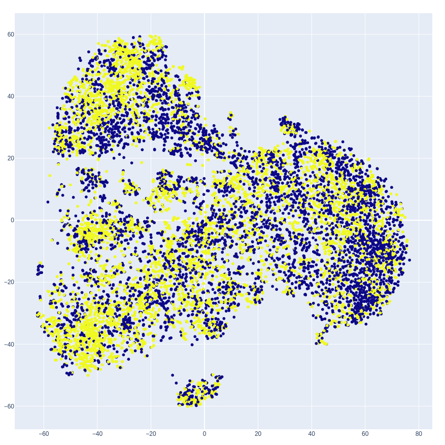
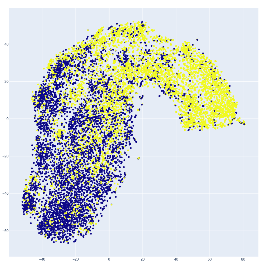
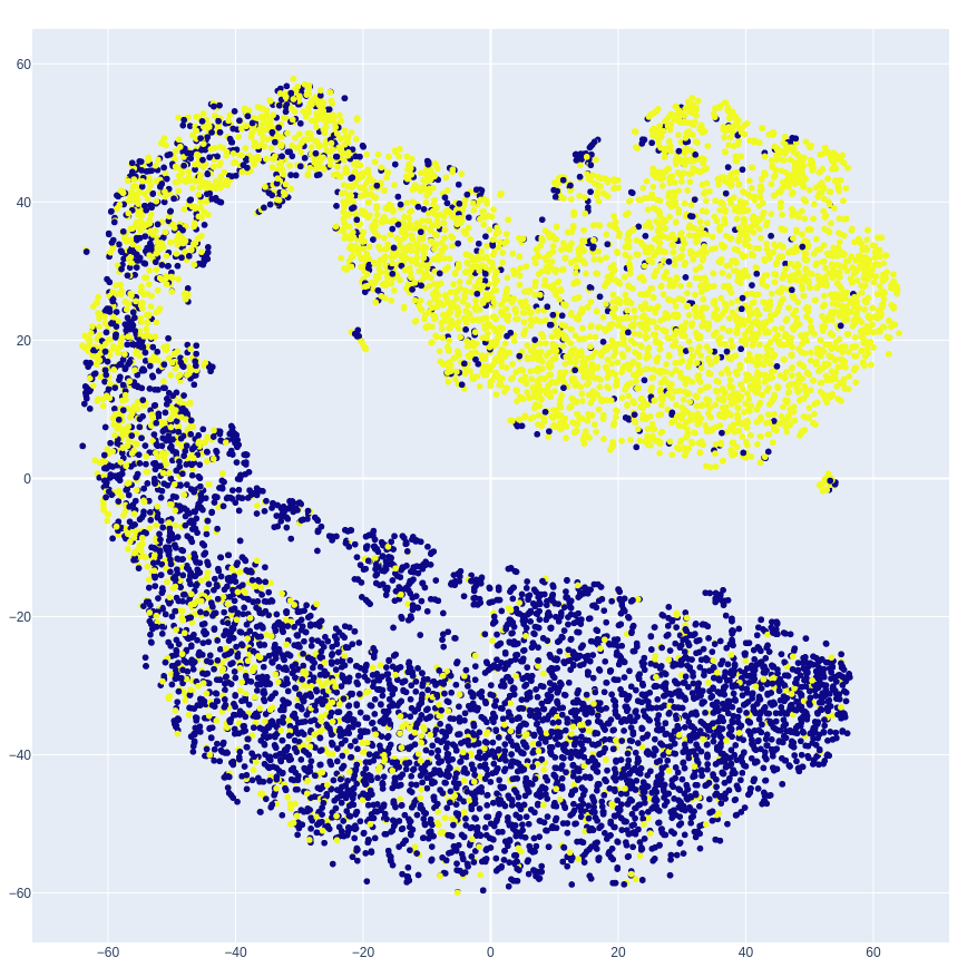
Figure 1: t-SNE visualization of [CLS] embeddings for few-shot models trained on 20 examples from the MR dataset with different loss functions. Colour represents sentiment: blue - negative, and yellow - positive. Left: cross-entropy (CCE), Middle: CCE + SupCon Loss, Right: CCE + SoftTriple Loss.

4 Experimental Results

4.1 Result Analysis

Table 3 presents our results separately for models trained on 20, 100 and 1,000 observations. The results show a baseline performance where the model was trained using only CCE loss compared to models trained on CCE + SupCon loss and CCE + SoftTriple loss.

4.1.1 20-element dataset

Models with the SoftTriple loss outperformed baseline and models with the SupCon loss in each case, giving an average gain of 6.23 percentage points over baseline and 2.61 percentage points over the SupCon approach. The most significant improvement over baseline was observed for the MR dataset and the SoftTriple loss model, almost 13.5 percentage points. On the other hand, the lowest improvement from baseline for the SoftTriple loss models is 2.29 percentage points for the MPQA dataset, while the SupCon showed a deterioration in performance from baseline on this dataset.

4.1.2 100-element dataset

The SofTriple loss models are better than the baseline model in every case, resulting in an average improvement of 1.85 percentage points. Moreover, the SoftTriple loss models outperform the SupCon loss models in every case, except for the SST2 dataset, where the SupCon model is better than the SoftTriple by 0.35 percentage points. The largest improvement over baseline was observed for the MR set and the SoftTriple loss model and is 2.91 percentage points. On the other hand, the lowest improvement from baseline for the SoftTriple loss models is 0.67 percentage points for the SUBJ set.

4.1.3 1,000-element dataset

The SofTriple loss models are better than the baseline model in every case, resulting in an average improvement of 0.58 percentage points. Furthermore, the SoftTriple loss models outperform the SupCon loss models in every case, except for the TREC dataset, while in the case of SST2 the performance was the same. The largest improvement over baseline was observed for the MRPC set and the SoftTriple loss model and is 1.9 percentage points. On the other hand, the lowest improvement from baseline for the SoftTriple loss models is 0.67 percentage points for the SUBJ dataset. The average performance of the models trained using CCE loss combined with SoftTriple loss is higher than the baseline or models trained using CCE and SupCon loss.

4.2 Comprehensive Analysis

Among all the results, the largest percentage improvement of the F1 score compared to the baseline (CCE loss function) is for the MR dataset (+24% of relative difference, +13.48 of absolute difference). This section investigates sentiment analysis models trained in the few-shot scenarios on the smallest analyzed training dataset: 20 samples from the MR dataset. We conducted a comprehensive investigation to compare models’ results for those observations.

Table 5 summarizes various metrics proving that the proposed method (CCE + SoftTriple) outperforms other approaches (CCE, CCE + SupCon) on the MR dataset. Particularly, considerable progress has been made regarding the recall. In this case, CCE + SupCon achieves similar results to the base model (CCE), while values for CCE + SoftTriple differ significantly. Smaller values of standard deviation indicate that models with CCE + SoftTriple are more stable.

Figure 1 illustrates 2-dimensional representation of input text embeddings made with t-SNE algorithm van der Maaten and Hinton (2008). The baseline model (CCE) is not able to separate the different classes. Much better results are achieved with additional SupCon loss. However, the observations in the middle of the plot are not decoupled. SoftTriple loss helps to almost isolate two classes. Even 20 observations for fine-tuning the model are enough to achieve satisfactory results.

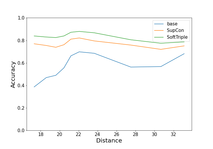
Figure 2: Relationship between accuracy and Euclidean distance between sentence embedding and mean embedding computed by baseline model with cross-entropy loss.

Figure 2 shows a difference in models’ performance depending on the chosen loss function. in this test, we defined a mean sentence embedding based on [CLS] representation from the model with cross-entropy loss. Then, we computed the Euclidean distance between the given observation and the mean embedding. The farther from the center, the greater the chance of being an outlier. Next, the observations were sorted according to the distance from the central embedding and divided into groups of equal size. The models’ accuracy was calculated in the designated groups and presented on the chart in Figure 2. Both models with additional SupCon and SoftTriple losses achieve better results than the base model with CCE. Results of models trained using DML show similar trend, but the SoftTriple is more accurate than the training with SupCon loss, even for observations far from the central embedding.

Table 6 presents examples of explainability with Shapley values Lundberg and Lee (2017). In Example 1, all the models predict the correct negative sentiment for the observation. The explanations of these models indicates that the same words increase the probability of the predicted class for all analyzed models. Intuitively, the word terrible has a big influence on this prediction. Surprisingly, word painful increases the probability of negative sentiment only for model with CCE + SoftTriple loss. Other models treat this word as neutral.

In Example 2, in Table 6, we present an observation that all analyzed models classified incorrectly as positive sentiment. Interestingly, the statement consists of word puzzling whose sentiment can be interpreted differently depending on context. Model trained with SupCon loss function treats this word as positive while the sentiment of this word measured with other models is slightly more negative.

Table 6: A Shapley values for each token for samples from MR dataset for a model trained on 20 samples. Red shades mean that a word increases the likelihood of positive sentiment, while blue shades mean an increase in the probability of a negative class.

Example 1
Loss function	Sentiment
cross-entropy	positive
SupCon	negative
SoftTriple	negative
ground-truth	negative

Example 2
Loss function	Sentiment
cross-entropy	positive
SupCon	positive
SoftTriple	positive
ground-truth	negative

Additionally, we performed test set analysis with geval method Graliński et al. (2019). This methods searches features that lower the evaluation metric in which it cannot be ascribed to a chance, measured by their p-values of Mann-Whitney rank U test. Table 7 shows a few groups of input observations that are particularly difficult for our models. For example, one group contains all the observations from the test set that contains the "but" word. Here, in sentiment analysis, even one word "but" can change the whole sentence sense and the model result, e.g. "Its premise is smart, but the execution is pretty weary." Still, even for those hard groups of input examples, the SubCon is better than the baseline (CCE), and the SoftTriple achieved the best performance.

Table 7: Accuracy of the three tested loss function in model training: CCE, CCE+SubCon, CCE+SoftTriple, for groups of input examples with a given characteristic, e.g. all the input examples containing a word "will".

Sample group	# examples	CCE	CCE+SupCon	CCE+SoftTriple
"n’t"	884	52	71	78
"but"	1613	55	0.72	76
"if"	524	52	70	74
"you"	880	52	66	72
"more"	685	54	72	79
"will"	349	53	69	73
Accuracy in the whole test set		58	77	83

5 Conclusion

This paper investigated the impact of using DML loss functions on supervised fine tuning language models by comparing the results of RoBERTa-large trained with raw cross-entropy loss function and training procedure enriched with distance metrics: SupCon and SoftTriple loss. The performance of the models was tested based on 40-fold cross-validation over multiple datasets from the SentEval Transfer Tasks. We found that the use of these functions improves the performance of the model, and the improvement is greater the smaller the dataset is. Applying SoftTriple loss increases the performance over baseline on average by about 2.89 percentage points, from 0.04 to 13.48 percentage points which is superior comparing to the average 1.62 percentage points from -0.22 to 9.19 percentage points for the SupCon. We would like to acknowledge that most of the results for which p-value is less than 0.05 belong to few-shot learning scenarios (20-element datasets, 100-element datasets), which is consistent with the results from previous work Gunel et al. (2020).

The comprehensive analysis of few-shot models’ performance on sentiment analysis task from the MR dataset revealed that enriching training procedure with DML methods (both SupCon and SoftTriple) cause an increase in model accuracy. Model fitted with SofTriple loss achieved higher scores for all analysed metrics (F1 score, accuracy, recall, precision, and AUC). Moreover, t-SNE visualizations point towards the idea that our method separates classes better than other models even for 20 training observations.

References

- Vaswani et al. [2017] Ashish Vaswani, Noam Shazeer, Niki Parmar, Jakob Uszkoreit, Llion Jones, Aidan N Gomez, Łukasz Kaiser, and Illia Polosukhin. Attention is all you need. In NeurIPS, pages 5998–6008, 2017.
- Devlin et al. [2019] Jacob Devlin, Ming-Wei Chang, Kenton Lee, and Kristina Toutanova. Bert: Pre-training of deep bidirectional transformers for language understanding. ArXiv, abs/1810.04805, 2019.
- Bansal et al. [2019] Trapit Bansal, Rishikesh Jha, and Andrew McCallum. Learning to few-shot learn across diverse natural language classification tasks. arXiv preprint arXiv:1911.03863, 2019.
- Zhang et al. [2020] Tianyi Zhang, Felix Wu, Arzoo Katiyar, Kilian Q Weinberger, and Yoav Artzi. Revisiting few-sample bert fine-tuning. arXiv preprint arXiv:2006.05987, 2020.
- Wen et al. [2016] Yandong Wen, Kaipeng Zhang, Zhifeng Li, and Yu Qiao. A discriminative feature learning approach for deep face recognition. In ECCV, pages 499–515, 2016.
- Cao et al. [2019] Kaidi Cao, Colin Wei, Adrien Gaidon, Nikos Arechiga, and Tengyu Ma. Learning imbalanced datasets with label-distribution-aware margin loss. NeurIPS, 32, 2019.
- Qian et al. [2019] Qi Qian, Lei Shang, Baigui Sun, Juhua Hu, Hao Li, and Rong Jin. Softtriple loss: Deep metric learning without triplet sampling. In IEEE/CVF, pages 6450–6458, 2019.
- Weinberger and Saul [2009] Kilian Q Weinberger and Lawrence K Saul. Distance metric learning for large margin nearest neighbor classification. JMLR, 10(2), 2009.
- Xing et al. [2002] Eric Xing, Michael Jordan, Stuart J Russell, and Andrew Ng. Distance metric learning with application to clustering with side-information. NeurIPS, 15, 2002.
- Hadsell et al. [2006] Raia Hadsell, Sumit Chopra, and Yann LeCun. Dimensionality reduction by learning an invariant mapping. In CVPR, volume 2, pages 1735–1742. IEEE, 2006.
- Schroff et al. [2015] Florian Schroff, Dmitry Kalenichenko, and James Philbin. Facenet: A unified embedding for face recognition and clustering. In CVPR, pages 815–823, 2015.
- Pereyra et al. [2017] Gabriel Pereyra, George Tucker, Jan Chorowski, Łukasz Kaiser, and Geoffrey Hinton. Regularizing neural networks by penalizing confident output distributions. arXiv:1701.06548, 2017.
- Khosla et al. [2020] Prannay Khosla, Piotr Teterwak, Chen Wang, Aaron Sarna, Yonglong Tian, Phillip Isola, et al. Supervised contrastive learning. arXiv preprint arXiv:2004.11362, 2020.
- Gunel et al. [2020] Beliz Gunel, Jingfei Du, Alexis Conneau, and Ves Stoyanov. Supervised contrastive learning for pre-trained language model fine-tuning. arXiv preprint arXiv:2011.01403, 2020.
- Liu et al. [2019] Yinhan Liu, Myle Ott, Naman Goyal, Jingfei Du, Mandar Joshi, Danqi Chen, et al. Roberta: A robustly optimized bert pretraining approach. arXiv preprint arXiv:1907.11692, 2019.
- Wu et al. [2016] Yonghui Wu, Mike Schuster, Zhifeng Chen, Quoc V Le, Mohammad Norouzi, et al. Google’s neural machine translation system: Bridging the gap between human and machine translation. arXiv preprint arXiv:1609.08144, 2016.
- Dvornik et al. [2019] Nikita Dvornik, Cordelia Schmid, and Julien Mairal. Diversity with cooperation: Ensemble methods for few-shot classification. In IEEE/CVF, pages 3723–3731, 2019.
- Conneau and Kiela [2018] Alexis Conneau and Douwe Kiela. Senteval: An evaluation toolkit for universal sentence representations. arXiv preprint arXiv:1803.05449, 2018.
- Socher et al. [2013] Richard Socher, Alex Perelygin, Jean Wu, et al. Recursive deep models for semantic compositionality over a sentiment treebank. In EMNLP, pages 1631–1642, 2013.
- Pang and Lee [2005] Bo Pang and Lillian Lee. Seeing stars: Exploiting class relationships for sentiment categorization with respect to rating scales. arXiv preprint cs/0506075, 2005.
- Wiebe et al. [2005] Janyce Wiebe, Theresa Wilson, and Claire Cardie. Annotating expressions of opinions and emotions in language. Language resources and evaluation, 39(2):165–210, 2005.
- Pang and Lee [2004] Bo Pang and Lillian Lee. A sentimental education: Sentiment analysis using subjectivity summarization based on minimum cuts. arXiv preprint cs/0409058, 2004.
- Hu and Liu [2004] Minqing Hu and Bing Liu. Mining and summarizing customer reviews. In ACM SIGKDD, pages 168–177, 2004.
- Dolan et al. [2004] William Dolan, Chris Quirk, Chris Brockett, and Bill Dolan. Unsupervised construction of large paraphrase corpora: Exploiting massively parallel news sources, 2004.
- van der Maaten and Hinton [2008] Laurens van der Maaten and Geoffrey E. Hinton. Visualizing data using t-sne. JMLR, 9:2579–2605, 2008.
- Lundberg and Lee [2017] Scott M Lundberg and Su-In Lee. A unified approach to interpreting model predictions. In NeurIPS, pages 4765–4774. Curran Associates, Inc., 2017.
- Graliński et al. [2019] Filip Graliński, Anna Wróblewska, Tomasz Stanisławek, Kamil Grabowski, and Tomasz Górecki. Geval: Tool for debugging nlp datasets and models. pages 254–262. ACL, 2019.