Most probable paths for developed processes

Abstract.

Optimal paths for the classical Onsager-Machlup functional determining most probable paths between points on a manifold are only explicitly identified for specific processes, for example the Riemannian Brownian motion. This leaves out large classes of manifold-valued processes such as processes with parallel transported non-trivial diffusion matrix, processes with rank-deficient generator and sub-Riemannian processes, and push-forwards to quotient spaces. In this paper, we construct a general approach to definition and identification of most probable paths by measuring the Onsager-Machlup functional on the anti-developement of such processes. The construction encompasses large classes of manifold-valued process and results in explicit equation systems for most probable paths. We define and derive these results and apply them to several cases of stochastic processes on Lie groups, homogeneous spaces, and landmark spaces appearing in shape analysis.

1. Introduction

The Onsager-Machlup functional [10] identifies most probable paths between points on manifolds for certain diffusion processes. The functional measures the probability that a process sojourns in $\varepsilon$-tubes around differentiable paths in the $\varepsilon\to 0$ limit. First covering the Euclidean space Brownian motion, the Onsager-Machlup functional has been derived for Brownian motions on Riemannian manifolds [17, 18] with extension to e.g. time-inhomegenous diffusions [8] and pinned-diffusions [13]. Most probable paths and the Onsager-Machlup functional have also been treated in infinite dimensional manifolds [9, 6, 3, 12]. Still, only limited classes of manifold-valued processes are covered in the literature: Processes with parallel transported diffusion matrix, sub-Riemannian processes, push-forwards through a projection from, for example, a Lie group to a homogeneous space, and many infinite dimensional non-linear shape processes are not among these.

Large classes of manifold-valued processes can be constructed by development of Euclidean semi-martingales to the manifold. Inspired by the constructions in [16, 12] that define most probable paths for anisotropic (non-Markovian) diffusion processes using the Onsager-Machlup functional on the anti-development of the processes, we here construct a general approach to defining and identifying most probable paths for processes that are constructed by development. This allows to derive differential equation systems for the resulting paths that both identify the set of most probable paths and allows numerical integration. The fundamental idea is to look at paths around which the anti-developed process sojourns.

We exemplify the results in several cases that are important in applications, including invariant processes on Lie groups and their push-forwards to homogeneous spaces, and, in the infinite dimensional case, paths of diffemorphisms between landmark configurations as often encountered in shape analysis [19]. Stochastic shape analysis has applications in medical imaging and biology, and the presented results allows to find the most probable transformations between e.g. a species shape and its immediate evolutionary ancestor compared to the geodesic transformations that are currently most used in shape analysis and where stochasticity is not taken into account.

1.1. Outline

In Section 2, we set the context, survey the fundamental constructions used in the paper including development and anti-development of processes and prove the first result on variations of curves and development. Section 3 contains the main results of the paper with the general equations for most probable paths for developed processes. We treat multiple particular cases in Section 4. In Section 5, we cover paths the results as projections through subjective submersions and where the dynamics can be lifted to the top space, e.g. homogeneous spaces. Section 6 covers Sobolev diffeomorphis and actions on those on landmark spaces as appearing in shape analysis. We end the paper with numerical examples on several manifolds in Section 7.

2. Affine transport and most probable paths

In this section, we will make precise the context of developed processes, state general assumptions and derive first results linking the variation of curves with variations of their development. This provides the foundation of the identification of most probable paths in the following sections.

2.1. Affine transport

Let $M$ be a manifold of dimension $d$ with a connection $\nabla$ and $o\in M$ a chosen point. Affine connections give us a correspondence between curves in $T_{o}M$ starting at $0$ and curves in $M$ starting at $o$. For a smooth curve $[0,T]\to T_{o}M$, $t\mapsto\omega_{t}$ with $\omega_{0}=0$, we define its development $\gamma:[0,T]\to M$ as the solution to

$$\dot{\gamma}_{t}=/\!/_{t}\dot{\omega},\quad\gamma_{0}=o,$$

where $/\!/_{t}:T_{o}M\to T_{\gamma_{t}}M$ denotes parallel transport along $\gamma_{t}$ with respect to $\nabla$. We call $\omega_{t}$ anti-development of $\gamma_{t}$. Any curve $\gamma_{t}$ has an anti-development. Conversely, any curve $\omega$ has a development if $\nabla$ is complete. For the remainder of the paper, we will assume that all connections are complete. For modifications when $\nabla$ is not complete, see [7, Remark 2.2].

In this paper, we are considering an affine analogue of the concept of development. Let $u_{t}$ be a time-dependent vector field. For a smooth curve $\omega_{t}$ starting at $0$, we define the affine development of $(\nabla,u_{t})$ as the solution of

$$\dot{\gamma}_{t}=/\!/_{t}\dot{\omega}_{t}+u_{t}(\gamma_{t}),\qquad\gamma_{0}=o.$$

Again, this exists for any smooth $\omega_{t}$ if $\nabla$ and $u_{t}$ are complete. We write $\gamma_{t}=\operatorname{Dev}_{u}(\omega)_{t}$.

We will now produce a generalization of a result in [7, Lemma 2.1] given for the derivative of the development map. We will first introduce the following notation. If $\tau_{t}$ is a time-dependent $\binom{i}{j}$-tensor and $\gamma_{t}$ is a curve in $M$, we define $\tau_{t,/\!/_{t}}:(T_{o}M)^{\otimes i}\otimes(T_{o}^{*}M)^{\otimes j}\to\mathbb{R}$ as the corresponding linear map defined by parallel transporting all elements to $o=\gamma_{0}\in M$. For example, if $T$ and $R$ are respectively the torsion and the curvature of $\nabla$, then

$$T_{/\!/_{t}}(v,w)=/\!/_{t}^{-1}T(/\!/_{t}v,/\!/_{t}w),\qquad R_{/\!/_{t}}(v,w)=/\!/_{t}^{-1}R(/\!/_{t}v,/\!/_{t}w)/\!/_{t},$$

for any $v,w\in T_{o}M$, while $u_{t,/\!/_{t}}=/\!/_{t}^{-1}u_{t}$. We now have the following result.

Lemma 2.1.

Let $k_{t}$ be a smooth map in $T_{o}M$ satisfying $k_{0}=0$. Then

$$\frac{d}{ds}\operatorname{Dev}_{u}(\omega+sk)_{t}|_{s=0}=/\!/_{t}v_{t},$$

where $v_{t}$ is the solution of $v_{0}=0$ and

(2.1) $$k_{t} =v_{t}-\int_{0}^{t}/\!/_{s}^{-1}\nabla_{/\!/_{s}v_{s}}u_{s}ds-\int_{0}^{t}T_{/\!/_{s}}(\dot{\omega}_{s}+u_{s,/\!/_{s}},v_{s})ds$$

$$\qquad-\int_{0}^{t}\int_{0}^{s}R_{/\!/_{r}}(\dot{\omega}_{r}+u_{r,/\!/_{r}},v_{r})\dot{\omega}_{s}\,drds.$$

Proof.

Write $\gamma_{t}^{s}=\operatorname{Dev}_{u}(\omega+sk)_{t}$. Construct a basis $e_{1,t}^{s},\dots,e^{s}_{d,t}$ of vector fields along $\gamma_{t}^{s}$ uniquely determined by their initial conditions and $D_{t}e_{j,t}^{s}=0$. We use the standard formulas,

$$T(\partial_{s}\gamma_{t}^{s},\partial_{t}\gamma_{t}^{s}) =\frac{D}{ds}\partial_{t}\gamma_{t}^{s}-\frac{D}{dt}\partial_{s}\gamma_{t}^{s},$$

$$R(\partial_{t}\gamma_{t}^{s},\partial_{s}\gamma_{t}^{s})e_{j,t}^{s} =\frac{D}{dt}\frac{D}{ds}e_{j,t}^{s}-\frac{D}{ds}\frac{D}{dt}e_{j,t}^{s}=\frac{D}{dt}\frac{D}{ds}e_{j,t}^{s}.$$

If we write $k_{t}=\sum_{j=1}^{d}k_{t}^{j}e_{j,0}$, $\omega_{t}=\sum_{j=1}^{d}\omega_{t}^{j}e_{j,0}$ and $\partial_{s}\gamma_{t}|_{s=0}=/\!/_{t}v_{t}$, then

$$\dot{v}_{t}=/\!/_{t}^{-1}\frac{D}{dt}\partial_{s}\gamma_{t}^{s}|_{s=0}=/\!/_{t}^{-1}\left.\left(\frac{D}{ds}\partial_{t}\gamma_{t}^{s}-T(\partial_{s}\gamma_{t}^{s},\partial_{t}\gamma_{t}^{s})\right)\right|_{s=0}$$

$$=/\!/_{t}^{-1}\left(\sum_{i=1}^{d}\dot{k}^{i}_{t}e_{j,t}+\sum_{i=1}^{n}\dot{\omega}^{j}_{t}\frac{D}{ds}e_{j,t}^{s}|_{s=0}+(\nabla_{/\!/_{t}v_{t}}u_{t})(\gamma_{t})-T(/\!/_{t}v_{t},/\!/_{t}\omega_{t}+u_{t}(\gamma_{t}))\right)$$

$$=\dot{k}_{t}+\sum_{i=1}^{n}\dot{\omega}^{j}_{t}\frac{D}{ds}e_{j,t}^{s}|_{s=0}+/\!/_{t}^{-1}(\nabla_{/\!/_{t}v_{t}}u_{t})(\gamma_{t})-T_{/\!/_{t}}(v_{t},\omega_{t}+/\!/_{t}^{-1}u_{t}(\gamma_{t}))$$

Furthermore,

$$\frac{d}{dt}/\!/_{t}^{-1}\frac{D}{ds}e_{j,t}^{s}|_{s=0} =/\!/_{t}^{-1}\frac{D}{dt}\frac{D}{ds}e_{j,t}^{s}|_{s=0}=/\!/_{t}^{-1}R(\partial_{t}\gamma_{t}^{s},\partial_{s}\gamma_{t}^{s})e_{j,t}^{s}|_{s=0}$$

$$=R_{/\!/_{t}}(\dot{\omega}_{t}+/\!/_{t}^{-1}u_{t}(\gamma_{t}),v_{t})e_{j}$$

Since $D_{s}e_{j,t}^{s}|_{s=0,t=0}=0$ by definition, we have

$$\frac{D}{ds}e_{j,t}^{s}|_{s=0}=/\!/_{t}\int_{0}^{t}R_{/\!/_{r}}(\dot{\omega}_{r}+/\!/_{r}^{-1}u_{r}(\gamma_{r}),v_{r})e_{j}dr.$$

Using that also $v_{0}=0$, the result follows. ∎

2.2. Diffusion processes with drift and non-zero covariance

Let $o\in M$ be a reference point and let $\langle\cdot,\cdot\rangle$ be a reference inner product on $T_{o}M$. For now, the choice of inner product is not important, as all inner products give Lipschitz equivalent norms on finite dimensional vector spaces. For a given $T>0$, define the Cameron Martin space $\mathbb{H}^{T}(T_{o}M)$ as the space of all absolutely continuous curves in $T_{o}M$ starting at $0$ with an $L^{2}$-derivative with respect to our chosen inner product. This is a Hilbert space with product

$$\langle\omega,k\rangle_{\mathbb{H}}=\int_{0}^{T}\langle\dot{\omega}_{t},\dot{k}_{t}\rangle\,dt.$$

We notice that the concept of affine development $\operatorname{Dev}_{u}(\omega)$ is well defined for curves $\omega\in\mathbb{H}^{T}(T_{o}M)$, and we can still apply Lemma 2.1 with its proof. See Appendix B for details.

Let $\sigma_{1,t}$, $\dots$, $\sigma_{J,t}$ be smooth, time-dependent vectors in $T_{o}M$. We consider a process $x_{t}$ in $M$ with $x_{0}=o$ as the solution of

$$dx_{t}=/\!/_{t}\sum_{j=1}^{J}\sigma_{j,t}\circ d\hat{B}^{j}_{t}+u_{t}(x_{t})\,dt,$$

where $(\hat{B}_{t}^{1},\dots,\hat{B}_{t}^{J})$ is a standard Brownian motion in $\mathbb{R}$ and $/\!/_{t}:T_{o}M\to T_{x_{t}}M$ denotes parallel transport along $x_{t}$. If we introduce the map $\Sigma_{t}:T_{o}M\to T_{o}M$ by $\Sigma_{t}v=\sum_{j=1}^{J}\langle\sigma_{t},v\rangle\sigma_{t}$, then we can write $x_{t}$ as the solution of

(2.2) $$dx_{t}=/\!/_{t}\Sigma_{t}^{1/2}\circ dB_{t}+u(x_{t})\,dt,$$

where now $B_{t}$ is a standard Brownian motion in the inner product space $(T_{o}M,\langle\cdot,\cdot\rangle)$.

To the best of our knowledge, there are no general expression for the Onsager-Machlup functional for $x_{t}$ even in the case when $\Sigma_{t}=\Sigma$ is constant in time and of full rank, but not the identity, and with $u_{t}=0$. As such, with slight abuse of terminology, we introduce the following replacement. For any $y\in M$, we define $\mathbb{H}(y)=\mathbb{H}^{T}(T_{o}M;\nabla,\Sigma_{t},u_{t},y)$ as the subset of all curves $\omega_{t}$ such that if $\gamma_{t}$ is the solution of

(2.3) $$\dot{\gamma}_{t}=/\!/_{t}\Sigma_{t}^{1/2}\dot{\omega}_{t}+u_{t}(\gamma_{t}),\qquad\gamma_{0}=o.$$

then

(2.4) $$\Pi(\omega):=\gamma_{T}=y.$$

We then say that $\gamma_{t}$ is a most probable path from $o$ to $y$ if $\omega$ is the most probable path in $\mathbb{H}(y)$ with respect to $B_{t}$.

We will introduce the following to simplifying assumptions. Let $\operatorname{Hol}_{o}$ denote the holonomy group of $\nabla$ at $o\in M$.

(A) $$\operatorname{image}\Sigma_{t}=\mathfrak{e} t$$ is constant for any .

(B) $$\begin{split}&\text{Any element in $\operatorname{Hol}_{o}$ maps $\mathfrak{e}$ into itself}\\ &\text{and preserves an inner product $\langle\cdot,\cdot\rangle$ on $\mathfrak{e}$.}\end{split}$$

From these assumptions, we can do as follows. First, in (2.2) we can now consider $\Sigma_{t}$ and the Brownian motion $B_{t}$ as being defined only with respect to $\mathfrak{e}$ and its inner product, and $\omega\in\mathbb{H}^{T}(\mathfrak{e})$ only being in the Cameron-Martin space of $\mathfrak{e}$. The assumption (A) also means that $\Sigma_{t}$ is invertible as a map from $\mathfrak{e}$ to itself. Next, from (B), we now that there exists a subbundle $E\subseteq TM$ defined by parallel transport of $\mathfrak{e}$ and parallel transport also gives us a smooth inner product $g$ on $E$. The pair $(E,g)$ is called a sub-Riemannian structure. The connection $\nabla$ will be compatible with the sub-Riemannian structure, in the sense that orthonormal frames are parallel transported to orthonormal frames. With these assumptions, we can make our statement of equations for most probable paths, found in Theorem 3.1.

We will first, however, present the following useful lemma. Introduce a tensor $K$ seen as a map $K:\wedge^{2}E\otimes TM\to T^{*}M$ and defined by

(2.5) $$K(v_{1},v_{2},w_{1})(w_{2})=K(v_{1}\wedge v_{2},w_{1})(w_{2})=\langle R(w_{1},w_{2})v_{1},v_{2}\rangle_{g}.$$

Here we have used that the connection $\nabla$ is compatible with the sub-Riemannian structure $(E,g)$ and hence the right hand side of (2.5) is skew-symmetric in $v_{1}$ and $v_{2}$. We will also need the map $\sharp^{g}:T^{*}M\to E$ defined such that if

$$\alpha(v)=\langle\sharp^{g}\alpha,v\rangle_{g},\qquad\text{for any $\alpha\in T^{*}M$, $v\in E$, $x\in M$.}$$

Relative to this notation, we have the following result.

Lemma 2.2.

Let $\omega,k\in\mathbb{H}^{T}(\mathfrak{e})$ be arbitrary and define $\gamma_{t}^{s}=\operatorname{Dev}_{u}(\omega+sk)$ and $\frac{d}{ds}\gamma_{t}^{s}|_{s=0}=/\!/_{t}v_{t}$. Then for any absolutely continuous curve $\lambda_{t}$ along $\gamma_{t}$, we have

$$\int_{0}^{T}\lambda_{t}(/\!/_{t}\dot{k}_{t})\,dt=\lambda_{T}(/\!/_{T}v_{T})-\int_{0}^{t}\alpha_{t}(/\!/_{t}v_{t})\,dt$$

where

$$\alpha_{t}=\frac{D}{dt}\lambda_{t}+\lambda_{t}(\nabla u_{t})+\lambda_{t}(T(\dot{\gamma}_{t},\cdot))-K(\chi_{t},\gamma_{t}),$$

and $\chi_{t}$ is the two-vector fields along $\gamma_{t}$ with values in $\wedge^{2}E$ that is the solution of

$$\frac{D}{dt}\chi_{t}=(\dot{\gamma}_{t}-u_{t}(\gamma_{t}))\wedge\sharp^{g}\lambda_{t},\qquad\chi_{T}=0.$$

Proof.

We use equation (2.1). Observe first that

$$\int_{0}^{T}\int_{0}^{t}\lambda_{t}/\!/_{t}R_{/\!/_{r}}(\dot{\omega}_{r}+u_{r,/\!/_{t}}(\gamma_{r}),v_{r})\dot{\omega}_{t}\,drdt$$

$$=\int_{0}^{T}\int_{t}^{T}\lambda_{r}/\!/_{r}/\!/_{t}^{-1}R(\dot{\gamma}_{t},/\!/_{t}v_{t})/\!/_{t}/\!/_{r}^{-1}(\gamma_{r}-u_{r}(\gamma_{r}))\,drdt$$

$$=-\int_{0}^{T}K(\chi_{t},\gamma_{t})(/\!/_{t}v_{t})dt,$$

meaning that

$$\int_{0}^{T}\lambda_{t}(/\!/_{t}\dot{k}_{t})\,dt =\int_{0}^{T}\lambda_{t}(/\!/_{t}\dot{v}_{t})\,dt-\int_{0}^{T}\lambda_{t}(\nabla_{/\!/_{t}v_{t}}u_{t})dt$$

$$\qquad-\int_{0}^{t}\lambda_{t}T(\dot{\gamma}_{t},/\!/_{t}v_{t})dt+\int_{0}^{T}K(\chi_{t},\gamma_{t})(/\!/_{t}v_{t})dt$$

$$=\lambda_{T}(/\!/_{T}v_{T})-\int_{0}^{t}\alpha_{t}(/\!/_{t}v_{t}),$$

by using integration by parts. ∎

2.3. Singular curves

If we consider the map $\Pi:\mathbb{H}^{T}(\mathfrak{e})\to M$, $\omega\mapsto\gamma_{T}$ as defined in (2.4), this is a smooth map of Hilbert manifolds, meaning that if $\Pi(\omega)=y$ and $\omega$ is a regular point of $\Pi$, then $\mathbb{H}(y)=\Pi^{-1}(y)$ has the structure of a Hilbert manifold close to $\omega$ by the implicit function theorem. We say that $\omega$ is regular if it is a regular point of $\Pi$ and we will otherwise call it singular. We say that a curve $\gamma_{t}$ is singular if it is the solution of (2.3) for a singular $\dot{\omega}$.

We have the following criterion for singular curves.

Lemma 2.3.

The curve $\gamma$ is singular if and only there is if a non-vanishing one-form $\lambda_{t}$ along $\gamma_{t}$, vanishing on $E_{\gamma_{t}}$ and satisfying

(2.6) $$\left\{\begin{split}\dot{\gamma}_{t}-u_{t}(\gamma_{t})\in E,\text{for almost every t},\\ \frac{D}{dt}\lambda_{t}+\lambda_{t}\nabla u_{t}+\lambda_{t}T(\dot{\gamma}_{t},\cdot)=0,\\ \lambda_{t}|_{E}=0\end{split}\right.$$

Proof.

Since the map $\omega\mapsto\int_{0}^{\cdot}\Sigma_{s}^{1/2}\dot{\omega}_{s}\,ds$ is an invertible map of $\mathbb{H}^{T}(\mathfrak{e})$, we only need to look as singular points of $\tilde{\Pi}(\omega)=\operatorname{Dev}_{u}(\omega)_{T}$. For $\omega,k\in\mathbb{H}^{T}(\mathfrak{e})$, let $v_{t}$ be defined as in (2.1), which gives us the relation $\tilde{\Pi}_{\omega,*}k=/\!/_{T}v_{T}$. Hence, $\gamma$ is singular if for some non-zero $\lambda_{T}\in T_{\Pi(\omega)}^{*}M$, we have that

$$\lambda_{T}/\!/_{T}v_{T}=0,$$

for all solutions $v_{t}$ of (2.1).

Consider now $\lambda_{t}$ as the unique one-form along $\gamma_{t}$ with final value $\lambda_{T}$ and that solves the equations

(2.7) $$\left\{\begin{split}\frac{D}{dt}\lambda_{t}&=-\lambda_{t}(\nabla u_{t})-\lambda_{t}(T(\dot{\gamma}_{t},\cdot))+K(\chi_{t},\gamma_{t}),\\ \frac{D}{dt}\chi_{t}&=(\gamma_{t}-u_{t}(\gamma_{t}))\wedge\sharp^{g}\lambda_{t},\qquad\chi_{T}=0.\end{split}\right.$$

It then follows that

$$\lambda_{T}(/\!/_{T}v_{T})=\int_{0}^{T}\lambda_{t}(/\!/_{t}\dot{k}_{t})\,dt.$$

Since $\dot{k}_{t}$ can be an arbitrary $L^{2}$-function in $\mathfrak{e}$, we must hence have that $\lambda_{t}$ vanishes on $E_{\gamma_{t}}=/\!/_{t}\mathfrak{e}$. Finally, we use that $\sharp^{g}\lambda_{t}=0$, giving us that $\chi_{t}=0$ and we have the result. ∎

Remark 2.4.

We mention in particular that if $\mathfrak{e}=T_{o}M$, then $\operatorname{Ann}(E)=0$ and there are no singular curves.

3. Equations for most probable paths

We are now ready to present our main result. Let $x_{t}$ be the solution of (2.2) for a given $\Sigma_{t}$ and $u_{t}$. In what follows, it will be practical to introduce the following abuse of notation, where we allow $\Sigma_{t}$ to act on elements in $E_{\gamma_{t}}$ by $\Sigma_{t}v=/\!/_{t}\Sigma_{t}/\!/_{t}^{-1}v$. With this terminology, we have the following equation for most probable paths.

Theorem 3.1.

If $\gamma:[0,T]\to M$ is a most probable path of $x_{t}$ and not singular, then it is the solution of

(3.1) $$\left\{\begin{split}\sharp^{g}\lambda_{t}&=\Sigma_{t}^{-1}(\dot{\gamma}_{t}-u_{t}(\gamma_{t}))\\ \frac{D}{dt}\lambda_{t}&=-\lambda_{t}(\nabla u_{t})-\lambda_{t}(T(\dot{\gamma}_{t},\cdot))+K(\chi_{t},\gamma_{t}),\\ \frac{D}{dt}\chi_{t}&=\frac{1}{2}\Sigma_{t}\sharp^{g}\lambda_{t}\wedge\sharp^{g}\lambda_{t},\qquad\chi_{T}=0.\end{split}\right.$$

Proof.

Assume that

$$\textstyle\gamma_{t}=/\!/_{t}\dot{\omega}_{2,t}+u_{t}(\gamma_{t}):=/\!/_{t}\int_{0}^{t}\Sigma_{r}^{1/2}\dot{\omega}_{r}\,dr+u_{t}(\gamma_{t})$$

and define $y=\gamma_{T}=\Pi(\omega)=\tilde{\Pi}(\omega_{2})$. Define vector spaces

$$V =\left\{\frac{d}{ds}\omega^{s}|_{s=0}\,:\text{$\omega^{s}$ is a variation of $\omega$, $\Pi(\omega^{s})=y$}\right\}$$

$$V_{2} =\left\{\frac{d}{ds}\omega_{2}^{s}|_{s=0}\,:\text{$\omega_{2}^{s}$ is a variation of $\omega_{2}$, $\tilde{\Pi}(\omega^{s}_{2})=y$}\right\}$$

Along the curve, also introduce the following vector space of forms

$$\Lambda=\{\text{$\lambda_{t}$ is a solution of \eqref{Pre-MPP}}\},$$

which is a $d$-dimensional space by definition with $d=\dim M$. Since $\gamma_{t}$ is not singular, $\lambda_{t}|_{E}$ cannot vanish for every $t$ for any non-zero $\lambda_{\cdot}\in\Lambda$ by Lemma 2.3. As a consequence

$$\textstyle\check{\Lambda}=\{\int_{0}^{t}/\!/_{r}^{-1}\sharp^{g}\lambda_{r}\,dr\}\subseteq\mathbb{H}^{T}(\mathfrak{e}).$$

is also a $d$-dimensional subspace. By Lemma  2.2

$$\textstyle\langle h_{t},k\rangle_{\mathbb{H}}=\int_{0}^{T}\lambda_{t}(/\!/_{t}k_{t})=0,\qquad\text{for $h=\int_{0}^{\cdot}/\!/_{r}^{-1}\sharp^{g}\lambda_{r}\,dr\in\check{\Lambda}$, and for any $k\in V_{2}$}.$$

Since $\check{\Lambda}$ is $d$-dimensional, it follows that $\mathbb{H}^{T}=\check{\Lambda}\oplus_{\perp}V_{2}$, and furthermore

$$\textstyle\mathbb{H}^{T}(\mathfrak{e})=\hat{\Lambda}\oplus_{\perp}V,\qquad\hat{\Lambda}=\{\int_{0}^{\cdot}\Sigma^{1/2}_{r}h_{r}\,dr\,:\,h\in\check{\Lambda}\}.$$

If $\gamma$ is a most probable path, then we must have

$$0=\frac{d}{ds}\operatorname{OM}(\omega^{s})=\int_{0}^{T}\langle\dot{\omega}_{t},k_{t}\rangle\,dt=\langle\omega,k\rangle_{\mathbb{H}},$$

for any $k\in V$, meaning that $\omega\in\hat{\Lambda}_{t}$. In conclusion, for some $\lambda_{t}$ in $\Lambda_{t}$, we must have that

$$/\!/_{t}^{-1}\sharp^{g}\lambda_{t}=\Sigma^{-1/2}_{t}\dot{\omega}_{t}=\Sigma_{t}^{-1}\dot{\omega}_{2,t}=\Sigma_{t}^{-1}/\!/_{t}(\gamma_{t}-u_{t}(\gamma_{t})).$$

The result follows. ∎

Remark 3.2.

Note that we cannot conclude (3.1) directly from Lemma 2.2 without the assumption that the curve is not singular, since the vector fields $t\mapsto/\!/_{t}v_{t}$ resulting from affine development will not be all vector fields when $E$ is strictly contained in $TM$. In fact, one can verify that if $\operatorname{pr}_{E}:TM\to E$ is any projection, then $v_{t}$ is uniquely determined by $\operatorname{pr}_{E}v_{t}$.

3.1. Optimal control point of view an minimal length curves

We note that finding our most probable paths can be formulated as an optimal control problem in the following way. We want to consider finding curves $\gamma_{t}$ solving (2.3) with final point $\gamma_{T}=y$ and minimizing $\operatorname{OM}(\omega_{t})=\frac{1}{2}\int_{0}^{T}\langle\dot{\omega}_{t},\dot{\omega}_{t}\rangle\,dt$ as an optimal control problem.

Assume that the bundle $E$ has rank $J$. Let $\operatorname{O}(J)\to\operatorname{O}(E)\stackrel{{\scriptstyle\pi}}{{\to}}M$ be the bundle of orthonormal frames of $E$. Recall that at each $y\in M$, $\operatorname{O}(E)$ consist of linear isometries $f=(f_{1},\dots,f_{J}):\mathbb{R}^{J}\to E_{y}$, with $\operatorname{O}(J)$ acting by compositions of the right. Let $f_{t}=(f_{1,t},\dots,f_{J,t})$ be an orthonormal frame of $E$ along the curve $\gamma_{t}$, defined on $(-\varepsilon,\varepsilon)$. Assume that each vector field $f_{j,t}$ is parallel along $\gamma_{t}$. We introduce the following notation

• If $\gamma_{0}=v\in E_{\gamma_{0}}$, we write $\dot{f}_{0}=h_{f_{0}}v$.

• We write $H_{j}(f_{0})=h_{f_{0}}f_{0,j}$.

Define a vector field $H_{j}:f\mapsto H_{j}(f)$ on $\operatorname{O}(E)$. If $X$ is a vector field on $M$, then we write $hX(f)=h_{f}X(\pi(f))$. We introduce notation $\dot{\omega}_{j,t}=\nu_{j,t}$ and let $f_{t}$ be a parallel curve along $\gamma_{t}$, where $\gamma_{t}$ is the solution of (2.3). If we include notation $\Sigma_{t}^{1/2}f_{j,0}=\sum_{i=1}^{J}(\Sigma^{1/2}_{t})_{ij}f_{i,0}$, then $f_{t}$ is the solution of

(3.2) $$\dot{f}_{t}=\sum_{i,j=1}^{J}(\Sigma_{t}^{1/2})_{ij}\nu_{j,t}H_{i}(f_{t})+hu_{t}(f_{t}).$$

We can consider (3.2) as a control system on $\operatorname{O}(E)$, and can consider the finding a most probable path as the result of finding an optimal control $\nu_{t}=(\nu_{1,t},\dots,\nu_{t})$ such that $f_{t}$ becomes a curve from $f_{0}$ to $\pi^{-1}(y)$ that minimize the cost functional $C(\nu)=\frac{1}{2}\int_{0}^{T}\langle\nu_{t},\nu_{t}\rangle\,dt$.

This can also be described in the following way. Let $\hat{E}\subseteq T\operatorname{O}(E)$ be the span of $H_{1},\dots,H_{J}$ and define $\hat{\rho}_{t}$ as the time-dependent sub-Riemannian metric on $\hat{E}$ such that $\sum_{i=1}^{J}(\Sigma_{t}^{1/2})_{ij}H_{i}$, $j=1,2,\dots,J$ form an orthonormal basis. A most probable path is then a projection of a curve $f_{t}$ from $f_{0}\in E_{0}$ to $\pi^{-1}(y)$ minimizing the energy

$$\tilde{\mathscr{E}}(f_{t})=\frac{1}{2}\int_{0}^{T}\left\|\dot{f}_{t}-hu_{t}(f_{t})\right\|_{\tilde{\rho}_{t}}^{2}\,dt.$$

If $u_{t}=0$ and $\tilde{\rho}_{t}=\tilde{\rho}$, such curves are length minimizing curves of the sub-Riemannian structure $(\hat{E},\hat{\rho})$.

While $\tilde{E}$ is projected to $E$ by $\pi_{*}$ bijectively on every fiber, the metric $\tilde{\rho}_{t}$ is in general not the pull-back of a time-dependent sub-Riemannian metric $\rho_{t}$ on $E$. We give two notable exceptions to this.

1. Isotropic covariance: If $\Sigma_{t}=c_{t}\operatorname{id}_{E_{o}}$, then $\tilde{\rho}_{t}=\pi^{*}\rho_{t}$ with $\rho_{t}=c_{t}^{-1}g$. This is reflected in equation (3.1) where $\chi_{t}=0$ if we have isotropic covariance.

2. Flat connection: If $\nabla$ is flat on $E$ and $M$ is simply connected, then parallel transport of $\Sigma_{t}$ is independent of path. Hence, we can parallel transport $\Sigma_{t}$ to every point giving us an endomorphism $\Sigma_{t}:E\to E$ which we denote by the same symbol. We then have that $\tilde{\rho}_{t}=\pi^{*}\rho_{t}$, with $\rho_{t}=g(\Sigma_{t}^{-1}\cdot,\cdot)$. This is reflected in equation (3.1) in that $K=0$ when $\nabla|E$ is flat, and hence $\chi_{t}$ play no role in this case. If $M$ is not simply connected, we still have the same identities locally.

If $\tilde{\rho}_{t}=\pi^{*}\rho_{t}$, then most probable paths are curves from $o$ to $y$ minimizing $\mathscr{E}(\gamma_{t})=\frac{1}{2}\int_{0}^{T}\|\dot{\gamma}_{t}-u_{t}(\gamma_{t})\|_{\rho_{t}}^{2}\,dt$.

Remark 3.3.

Considering the actual question of controllability, we know that if $u_{t}=u$ is independent of time, then we can find a curve $\dot{\gamma}_{t}=/\!/_{t}\int_{0}^{t}\Sigma_{s}^{1/2}\dot{\omega}_{s}\,ds+u(\dot{\gamma}_{t})$ connecting any pair of points if $E$ is bracket-generating by [4, Proposition 26]. We call $E$ bracket-generating if the sections of $E$ and its iterated brackets span the entire tangent bundle $TM$.

3.2. Change of connection

Since we have used the notion of anti-development to define our most-probable paths, we should verify that this indeed is invariant under our choices of structure to represent the equation.

First, consider the equation

$$dx_{t}=/\!/_{t}\int_{0}^{t}\Sigma_{t}^{1/2}\circ dB_{t}+u_{t}(\gamma_{t})dt,\qquad x_{0}=o\in M,$$

with respect to some a Brownian motion in $E_{o}$. Then the above equation is not changed if we replace the connection $\nabla$ with a different connection $\tilde{\nabla}_{X}Y:=\nabla_{X}Y+\mu_{X}Y$ where $X\mapsto\mu_{X}$ is a $TM$-edomorphism-valued one-form with the property that $\mu_{X}|E=0$. We verify that this is also the case for singular curves and most probable paths.

Proposition 3.4.

The solutions of (2.6) and (3.1) are the same for the connections $\nabla$ and $\tilde{\nabla}$.

Proof.

By definition, $K$ only depends on a the restriction of the connection to $E$, so it is sufficient to consider equation (2.6). Here we observe that

$$\frac{\tilde{D}}{dt}\lambda_{t}=\frac{D}{dt}\lambda_{t}-\lambda_{t}\mu_{\dot{\gamma}_{t}}$$

and since $\mu_{\cdot}\dot{\gamma}_{t}=\mu_{\cdot}u_{t}(\gamma_{t})$

$$-\lambda_{t}(\tilde{\nabla}u_{t})-\lambda_{t}\tilde{T}(\dot{\gamma}_{t},\cdot)$$

$$=-\lambda_{t}(\nabla u_{t})-\lambda_{t}(\mu_{\cdot}u_{t})-\lambda_{t}(T(\dot{\gamma}_{t},\cdot))-\lambda_{t}\mu_{\gamma_{t}}+\lambda_{t}(\mu_{\cdot}u_{t})$$

$$=-\lambda_{t}(\nabla u_{t})-\lambda_{t}(T(\dot{\gamma}_{t},\cdot))-\lambda_{t}\mu_{\gamma_{t}}$$

which clearly has the same solutions as (2.6). ∎

Lemma 3.5.

Let $\nabla$ and $\tilde{\nabla}$ be two connections that are compatible with the sub-Riemannian structure $(E,g)$ and let $u_{t}$ be a vector field. Let be the $\operatorname{Dev}_{u}$ and $\widetilde{\operatorname{Dev}}_{u}$ be the corresponding affine development. Then these maps have the same singular curves. Hence, the definition of singular curves, only depends on the triple $(E,g,u_{t})$.

Proof.

Let $\gamma_{t}$ be a curve that is singular, and let $\lambda_{t}$ be a one-form along $\gamma_{t}$ satisfying (2.6). If we write $\tilde{\nabla}_{X}Y=\nabla_{X}Y+\mu_{X}Y$, we then see that since $\sharp\lambda_{t}=0$, we have $\lambda_{t}(\mu_{X}\dot{\gamma})=\lambda_{t}(\mu_{X}u_{t})$ as $\mu_{X}(E)\subseteq E$ for any vector field $X$, since we are assuming that both connections are compatible with the sub-Riemannian structure. It follows that

$$\frac{\tilde{D}}{dt}\lambda_{t}+\lambda_{t}\tilde{\nabla}u_{t}+\lambda_{t}\tilde{T}(\dot{\gamma},\cdot)$$

$$=\frac{D}{dt}\lambda_{t}-\lambda_{t}\mu_{\dot{\gamma}}+\lambda_{t}\nabla u_{t}+\lambda_{t}\mu_{\cdot}u_{t}+\lambda_{t}T(\dot{\gamma},\cdot)+\lambda_{t}\mu_{\dot{\gamma}_{t}}-\lambda_{t}\mu_{\cdot}\dot{\gamma}_{t}=0.$$

Hence $\gamma_{t}$ is singular with respect to $\tilde{\nabla}$ as well. ∎

4. Examples

In this section, we consider several different examples, illustrating the different forms the equations for the most probable paths in Theorem 3.1 will take.

4.1. Riemannian and sub-Riemannian anisotropic Brownian motion

Let $(M,g)$ be a Riemannian manifold. For a given $o\in M$, let $B_{t}$ be the Brownian motion in $T_{o}M$. Write $\nabla$ for the Levi-Civita connection $g$. For a symmetric endomorphism $\Sigma:T_{o}M\to T_{o}M$, define $X_{t}$ as the solution of

(4.1) $$dx_{t}=/\!/_{t}\Sigma^{1/2}\circ dB_{t}.$$

We consider the most probable paths of this process.

Since $\operatorname{Ann}E=\operatorname{Ann}TM=0$, there are no singular curves and a most probable path is the solution of

$$\frac{D}{dt}\dot{\gamma}_{t}=\Sigma_{t}R(\chi_{t})\dot{\gamma},\qquad\frac{D}{dt}\chi_{t}=\frac{1}{2}\dot{\gamma}_{t}\wedge\Sigma_{t}\dot{\gamma}_{t},\qquad\chi_{T}=0.$$

These are exactly the equations found earlier in [12].

We can now consider a sub-Riemannian analogue, where we consider the equation (4.1) for a connection $\nabla$ that is compatible with $(E,g)$. Equations for the most probable path for non-singular curves are given by

$$\left\{\begin{split}\sharp^{g}\lambda_{t}&=\Sigma^{-1}\dot{\gamma}_{t}\\ \frac{D}{dt}\lambda_{t}&=-\lambda_{t}(T(\dot{\gamma},\cdot))+K(\chi_{t},\gamma_{t}),\\ \frac{D}{dt}\chi_{t}&=\frac{1}{2}\dot{\gamma}_{t}\wedge\Sigma^{-1}\dot{\gamma}_{t},\qquad\chi_{T}=0.\end{split}\right.$$

4.2. Lie groups with a right invariant structure

Let $G$ be a Lie group with Lie algebra $\mathfrak{g}$. Let $\mathfrak{e}\subseteq\mathfrak{g}$ be a subspace with an inner product $\langle\cdot,\cdot\rangle$ and define a sub-Riemannian structure $(E,g)$ by right translation. Let $\nabla$ be the right invariant connection on $G$, and recall that this is flat and with torsion such that $T(A,B)=[A,B]$ for any right invariant vector fields. Let $u_{t}$ be a vector field defined by right translation of a curve $a_{t}$ in $\mathfrak{g}$. Finally, consider symmetric transformation $\Sigma_{t}$. Let $B_{t}$ be a Brownian motion in $\mathfrak{e}$, and consider $x_{t}$ as the solution of $x_{0}=1_{G}$,

$$dx_{t}=/\!/_{t}\Sigma_{t}\circ dB_{t}+u_{t}(x_{t})\,dt=\circ dZ_{t}\cdot x_{t},$$

with $Z_{t}=\int_{0}^{t}\Sigma_{s}\circ dB_{s}+\int_{0}^{t}a_{s}ds$. The most probable paths are solutions of

(4.2) $$\left\{\begin{split}\dot{\gamma}_{t}&=z_{t}\cdot\gamma_{t},\\ \sharp^{g}\alpha_{t}&=\Sigma_{t}^{-1}(z_{t}-a_{t}),\\ \dot{\alpha}_{t}&=-(\operatorname{ad}(z_{t}))^{*}\alpha_{t},\end{split}\right.$$

where $z_{t}$ and $\alpha_{t}$ are respectively curves $\mathfrak{g}$ and $\mathfrak{g}^{*}$. Singular curves will be the curves where there is a non-trivial solution to

(4.3) $$\left\{\begin{split}\dot{\gamma}_{t}&=z_{t}\cdot\gamma_{t},\\ z_{t}-a_{t}&\in\mathfrak{e},\\ \sharp^{g}\alpha_{t}&=0,\\ \dot{\alpha}_{t}&=-(\operatorname{ad}(z_{t}))^{*}\alpha_{t}.\end{split}\right.$$

Remark 4.1.

If we replace right with left invariance in the above discussion, we get similar formulas but with $\operatorname{ad}$ replaced with $-\operatorname{ad}$.

4.3. Metrics invariant by a subgroup

We look at the following particular case of Section 4.2. Assume that $\mathfrak{g}=\mathfrak{e}\oplus\mathfrak{k}$ for some subalgebra $\mathfrak{k}$ and assume that $\mathfrak{g}$ has an inner product that is invariant under the adjoint action of $\mathfrak{k}$ and with $\mathfrak{e}=\mathfrak{k}^{\perp}$. It follows that $[\mathfrak{k},\mathfrak{e}]\subseteq\mathfrak{e}$. We will also assume that $[\mathfrak{e},\mathfrak{e}]\subseteq\mathfrak{k}$. We define a Riemannian metric $\bar{g}$ by left translation of the inner product on $\mathfrak{g}$. Write $E_{x}=x\cdot\mathfrak{e}$ and $g=\bar{g}|_{E}$. If we define $w_{t}=\sharp^{\bar{g}}\alpha_{t}=w_{\mathfrak{e},t}+w_{\mathfrak{k},t}$, then

$$\left\{\begin{split}\dot{\gamma}_{t}&=\gamma_{t}\cdot(\Sigma_{t}w_{\mathfrak{e},t}+a_{t})\\ \dot{w}_{\mathfrak{e},t}&=(\operatorname{ad}(\Sigma_{t}w_{\mathfrak{e},t}+a_{\mathfrak{e},t}))^{\dagger}w_{\mathfrak{k},t}+(\operatorname{ad}(a_{\mathfrak{k},t}))^{\dagger}w_{\mathfrak{e},t},\\ \dot{w}_{\mathfrak{k},t}&=(\operatorname{ad}(\Sigma_{t}w_{\mathfrak{e},t}+a_{\mathfrak{e},t}))^{\dagger}w_{\mathfrak{e},t}+(\operatorname{ad}(a_{\mathfrak{k},t}))^{\dagger}w_{\mathfrak{k},t},,\end{split}\right.$$

where $\operatorname{ad}(z)^{\dagger}$ is the adjoint with respect to $\langle\cdot,\cdot\rangle$.

4.4. Locally homogeneous spaces

If $u_{t}$, $R$ and $T$ are all parallel, we can solve the equations (3.1) at one point.

$$\left\{\begin{split}\dot{\gamma}_{t}&=/\!/_{t}(\Sigma_{t}\sharp^{g}\alpha_{t}+a_{t}),\qquad a_{t}=u_{t}(0)\\ \dot{\alpha}_{t}&=-\alpha_{t}(T(\Sigma_{t}\sharp^{g}\alpha_{t}+a_{t},\cdot))+K(\check{\chi}_{t},\Sigma_{t}\sharp^{g}\alpha_{t}+a_{t}),\\ \dot{\check{\chi}}_{t}&=\frac{1}{2}\Sigma_{t}\sharp^{g}\alpha_{t}\wedge\sharp^{g}\alpha_{t},\qquad\alpha_{T}=0.\end{split}\right.$$

5. Submersions

5.1. General submersions

Let $M$ be a manifold with a sub-Riemannian structure $(E,g)$. Let $\nabla$ be a connection compatible with the sub-Riemannian structure. Let $\Sigma_{t}:E_{o}\to E_{o}$ be a symmetric transformation of the space $E_{o}$ at $o\in M$. Relative to a time-dependent vector field, we define

$$dx_{t}=/\!/_{t}\Sigma_{t}^{1/2}\circ dB_{t}+u_{t}(x_{t})dt,\qquad x_{0}=o,$$

with $B_{t}$ being a Brownian motion in $E_{o}$. As before, we are studying curves $\gamma_{t}$ from $o$ to $y=\gamma_{T}=\Pi(\omega)$ solving $\dot{\gamma}_{t}=/\!/_{t}\Sigma_{t}^{1/2}\dot{\omega}_{t}+u_{t}(\gamma_{t})$ such that $\omega_{t}$ is most probable with respect to $B_{t}$.

Let $\pi:M\to N$ be a surjective submersion and write $\mathcal{V}=\ker\pi_{*}$ for the vertical space. We first note the following relation.

Lemma 5.1.

If $\check{\gamma}_{t}=\pi(\gamma_{t})$ is a curve from $\check{o}=\pi(o)$ to $\check{y}=\pi(y)=(\pi\circ\Pi)(\omega)$, and if $\omega$ is a regular point of $\pi\circ\Pi$ and a most probable path in $(\pi\circ\Pi)^{-1}(\check{y})$, then $\gamma_{t}$ is a solution (3.1) with $\lambda_{T}$ vanishing on $\mathcal{V}_{y}$

Proof.

This follows from considering the proof of Theorem 3.1, but with variations $\omega^{s}$ of $\omega$ such that if $\gamma_{t}^{s}=u_{t}(\gamma_{t}^{s})+/\!/_{t}^{s}\int_{0}^{r}\Sigma_{r}^{1/2}\dot{\omega}_{r}^{s}\,dr$, then $\frac{d}{ds}\gamma_{t}^{s}|_{s=0}\in\mathcal{V}_{y}$. ∎

We consider the following special case. For the surjective submersion $\pi:M\to N$, if $\check{y}\in N$, write $M_{\check{y}}=\pi^{-1}(\check{y})$. Let $(\check{E},\check{g})$ be a sub-Riemannian structure on $N$ such that $\pi_{*}|_{E}:E\to\check{E}$ is surjective with

$$\langle v,w\rangle_{g}=\langle v,w\rangle_{\check{g}},\qquad v,w\in\mathcal{H}=:(\mathcal{V}\cap E)^{\perp},$$

where the orthogonal complement is taken within $E$. We also assume that $\langle\Sigma_{t}v,w\rangle_{g}=\langle v,\Sigma_{t}w\rangle_{g}=0$ with $v\in\mathcal{H}$ and $w\in E\cap\mathcal{V}$.

For a vector $w\in\check{E}_{\check{y}}$ and $y\in M_{\check{y}}$, we define $h_{y}w$ as the unique element in $\mathcal{H}_{y}$ that projects to $w$. For a vector field $X$ with values in $\check{E}$, we define $hX(y)=h_{y}X(\pi(y))$. It then follows form our assumptions on $\Sigma_{t}$ that for any $v\in\mathcal{H}_{y}$, we have that

$$\Sigma_{t}v=h_{y}\check{\Sigma}_{t}\pi_{*}v,$$

for some symmetric map $\check{\Sigma}_{t}:\check{E}_{\check{y}}\to\check{E}_{\check{y}}$. Finally, we will assume that the following holds.

1. The vector field $u_{t}$ is $\pi$-related to a vector field $\check{u}_{t}$ on $N$, i.e. we have

   $$\pi_{*}u_{t}=\check{u}_{t}\circ\pi.$$

2. Identifying $\mathcal{H}$ with $\pi^{*}\check{E}$, we have that $\mathcal{H}$ is parallel with respect to $\nabla$ and furthermore, the restriction of $\nabla$ to $\mathcal{H}$ is the pull-back connection of $\check{\nabla}|\check{E}$ for some connection $\check{\nabla}$ on $N$ which is compatible with $(\check{E},\check{g})$. In other words, for any vector field $Y$ on $N$, we have

   (5.1) $$\ nabla_{v}hY=h\check{\nabla}_{\pi_{*}v}Y.$$

If we define $\check{x}_{t}=\pi(x_{t})$, we then have that

(5.2) $$d\check{x}_{t}=/\!\check{/}_{t}\check{\Sigma}_{r}^{1/2}\circ d\check{B}_{t}\,dr+\check{u}_{t}(\check{x}_{t})\,dt.$$

where $\pi_{*}B_{t}=\check{B}_{t}$ is a Brownian motion in $\check{E}_{\check{o}}$. We then have the following result

Proposition 5.2.

If $\check{\gamma}_{t}$ is a most probable path of $\check{x}_{t}$ starting at $\check{o}$ and not singular, then it is the projection of a solution $\gamma_{t}$ of (3.1) starting at $o$ with $\lambda_{0}$ vanishing on $\mathcal{V}_{o}$.

Proof.

Since $\mathcal{H}$ is parallel with respect to $\nabla$, this implies that $E^{\mathcal{V}}=E\cap\mathcal{V}$ is parallel from compatibility of the connection with the metric. Using Proposition 3.4, we are free to modify the connection $\nabla$ outside of $E\subseteq TM$. Choose a complement $\mathcal{P}$ to $\mathcal{V}$ such that $\mathcal{H}\subseteq\mathcal{P}$. With respect to $\mathcal{P}$, we have well-defined horizontal lifts for all elements in $TN$. Without loss of generality, we may assume that $\nabla$ on $\mathcal{P}$ is the pull-back connection of $\check{\nabla}$ on $TN$, in the sense that is satisfies (5.1) for horizontal lifts of all vector fields. We may also assume that $\mathcal{V}$ is parallel.

We note the following about the torsion of $\nabla$. Let $X$ and $Y$ be vector fields on $N$, while $V$ and $W$ are sections of $\mathcal{V}$. Let $\mathcal{R}$ be the curvature of $\mathcal{P}$, that is the tensor

(5.3) $$\mathcal{R}(hX+V,Y+W)=\operatorname{pr}_{\mathcal{V}}[hX,hY].$$

Since $hX$ and $hY$ are $\pi$-related to vector fields $X$ and $Y$ on $N$, we have

$$[hX,hY]=h[X,Y]+\mathcal{R}(hX,hY).$$

Furthermore, we note that $[hX,V]$ will be in $\mathcal{V}$ for any vector field $V$ with $\mathcal{V}$, since $V$ is then $\pi$-related to $0$. Because $\nabla$ is the pull-back connection on $\mathcal{P}$, $\nabla_{hX}hY=h\check{\nabla}_{X}Y$ and $\nabla_{V}hX=0$. From these identities, it follows that for vector fields $X$, $Y$ in $\mathcal{V}$ and vector fields $V$ and $W$ with values in $\mathcal{V}$,

$$T(hX,hY)=h\check{T}(X,Y)+\mathcal{R}(hX,hY),\qquad T(hX,V)|_{x},T(V,W)|_{x}\in\mathcal{V}.$$

In particular, if $\alpha\in T^{*}M$ vanishes on $\mathcal{V}$, then $\alpha(T(v,w))=\alpha(h\check{T}(\pi_{*}v,\pi_{*}w))$.

Write $u_{t}=h\check{u}_{t}+u^{\mathcal{V}}_{t}$. Let $(\check{\gamma}_{t},\check{\lambda}_{t},\check{\chi}_{t})$ is a solution to (3.1) on $N$. Define $(\gamma_{t},\lambda_{t},\chi_{t})$ by

$$\dot{\gamma}_{t} =h_{\gamma_{t}}(\dot{\check{\gamma}}_{t}-\check{u}_{t}(\check{\gamma}_{t}))+u_{t}(\gamma_{t}),$$

$$\lambda_{t} =\pi_{\gamma_{t}}^{*}\check{\lambda}_{t},$$

$$\chi_{t} =h_{\gamma_{t}}\check{\chi}_{t}.$$

By definition, $\sharp^{g}\lambda_{t}=\Sigma_{t}^{-1}(\dot{\gamma}-u_{t}(\gamma_{t}))$, $\frac{D}{dt}\chi_{t}=h_{\gamma_{t}}\frac{\check{D}}{dt}\chi_{t}=\Sigma_{t}\sharp^{g}\lambda_{t}\wedge\sharp^{g}\lambda_{t}$, and furthermore,

$$\frac{D}{dt}\lambda_{t}+\lambda_{t}(\nabla u_{t})+\lambda_{t}(T(\dot{\gamma}_{t},\cdot))+K(\chi_{t},\dot{\gamma}_{t})$$

$$=\pi^{*}_{\gamma_{t}}\frac{\check{D}}{dt}\check{\lambda}_{t}+\check{\lambda}_{t}(\check{\nabla}_{\pi_{t}}\check{u}_{t})+\check{\lambda}_{t}(\check{T}(\dot{\check{\gamma}}_{t},\pi_{*}\cdot)+\pi^{*}_{\gamma_{t}}\check{K}(\check{\chi}_{t},\dot{\check{\gamma}}_{t})=0.$$

This completes the result. ∎

With a similar approach, we have the following.

Proposition 5.3.

If the same assumptions as in Proposition 5.2, the curve $\check{\gamma}$ is singular if and only if it is a the projection of a solution of (2.6) with $\lambda_{0}$ vanishing on $E+\mathcal{V}$.

Remark 5.4.

For Proposition 5.2 and Proposition 5.3, if we are only interested in finding lifted formulas for singular curves and most probable paths on $N$, we can without loss of generality assume that $E=\mathcal{H}$, as $E\cap\mathcal{V}$ will play no role in the equations. We can also simplify to $u_{t}=h\check{u}_{t}$

5.2. Examples: Homogeneous spaces

As an example of submersion we consider a homogeneous space. Let $G$ be a Lie group with Lie algebra $\mathfrak{g}$. Let $\mathfrak{k}$ be a subalgebra corresponding to a closed subgroup $K$, and define $N=G/K$. We will assume that we have an inner product $\langle\cdot,\cdot\rangle$ on $\mathfrak{g}$. Write $\mathfrak{p}=\mathfrak{k}^{\perp}$ for the orthogonal complement of $\mathfrak{k}$. We observe that

$$\mathcal{V}_{x}=\ker\pi_{*,x}=x\cdot\mathfrak{k}.$$

If $A|_{1_{G}}\in\mathfrak{p}$ and $A$ is obtained by left-invariant translation, then $\pi_{*}A$ is non-vanishing, but only a vector field on $N$ if $A|_{1_{G}}$ is invariant under the action of $K$. On the other hand, $A$ is obtained by right translation of $A|_{1_{G}}\in\mathfrak{g}$, then $\pi_{*}A$ is a vector field on $N$, but may in general vanish at some points.

Example 5.5.

Assume that the inner product on $\mathfrak{g}$ is invariant under the adjoint action of $K$. Define $\mathcal{P}$ by left translation of $\mathfrak{p}$ and with a metric $g$ also obtained by left translation. Then for every $x\in G$, $\pi_{*,x}:\mathcal{P}_{x}\to T_{\pi(x)N}$ is an invertible map which induced a Riemannian metric $\check{g}$ on $TN$ by invariance under the action of $K$. Let $h_{x}v\in\mathcal{P}_{x}$ denote the horizontal lift of a vector $v\in T_{\check{x}}N$, $x\in\pi^{-1}(\check{x})$. Let $\nabla$ be a left connection on $G$ and let $\check{\nabla}$ be the connection on $M$ defined by

$$\nabla_{hX}hY=h\check{\nabla}_{X}Y.$$

If we define $\bar{X}:G\to\mathfrak{g}$ by $\bar{X}(a)=a^{-1}\cdot hX(a)$, then $\bar{X}(a\cdot k)=\operatorname{Ad}(k^{-1})\bar{X}(a)$.

Consider the vector field $\check{u}_{t}$ on $M$, $\check{\Sigma}_{t}:T_{o}M\to T_{o}M$ as a symmetric map and a Brownian motion $\check{B}_{t}$ in $T_{o}M$. We consider the process $\check{x}_{0}$ and a solution of

$$d\check{x}_{t}=/\!\check{/}_{t}\check{\Sigma}_{t}^{1/2}\circ d\check{B}_{t}+\check{u}_{t}(\check{x}_{t})\,dt.$$

Without loss of generality, we may assume that $\pi(1_{G})=o$. We can then consider $\pi(x_{t})=\check{x}_{t}$, with

$$dx_{t}=x_{t}\cdot\Sigma_{t}^{1/2}\circ dB_{t}+h\check{u}_{t}(x_{t})\,dt,$$

where $\Sigma_{t}$ is a symmetric map of $\mathfrak{p}$ and $B_{t}$ is a Brownian motion in $\mathfrak{p}$. Write $\bar{u}_{t}(a)=a^{-1}\cdot h\check{u}_{t}(a)$, which is $K$ invariant.

It follows that most probable paths in $N$ are projections of

(5.4) $$\left\{\begin{split}\dot{\gamma}_{t}&=\gamma_{t}\cdot z_{t},\qquad\gamma_{0}=1\\ z_{t}&=\Sigma_{t}\sharp^{g}\alpha_{t}+\bar{u}_{t}(\gamma_{t}),\\ \dot{\alpha}_{t}&=(\operatorname{ad}(z_{t}))^{*}\alpha_{t},\qquad\alpha_{0}|_{\mathfrak{k}}=0.\end{split}\right.$$

Example 5.6.

Consider now the case when $\tilde{\nabla}$ is a right invariant connection and define $(E,g)$ by right translation of a subspace $\mathfrak{e}\subseteq\mathfrak{p}$ and its inner product. We assume that there is a subbundle $\check{E}$ on $N$ such that $\pi_{*}E=\check{E}$ is well-defined and bijective on every fiber. This happens if $\operatorname{Ad}(x)\mathfrak{e}$ is transverse for $\mathfrak{k}$ for any $k$ in $G$. If this assumption holds, then if $A$ is a right invariant vector fields with values in $E$, then $\pi_{*}A$ is a non-vanishing vector field on $N$.

Let $a_{t}$ be a curve in $\mathfrak{g}$. Define $u_{t}$ as the vector field on $G$ obtained by right translation of $a_{t}$ and define $\check{u}_{t}=\pi_{*}u_{t}$ which is well defined at every point. Consider the stochastic process

$$dx_{t}=/\!/_{t}\Sigma_{t}\circ dB_{t}+u_{t}(x_{t})\,dt.$$

Let $\nabla$ be a connection on $N$ such that $\pi_{*}A$ is parallel for any right-invariant vector field. Then for $\check{x}_{t}=\pi(x_{t})$ is the solution of

$$dx_{t}=/\!/_{t}\check{\Sigma}_{t}\circ d\check{B}_{t}+\check{u}_{t}(x_{t})\,dt,$$

with $\check{B}_{t}=\pi_{*,o}B_{t}$ is a Brownian motion in $\check{E}_{\check{o}}$ and with $\check{\Sigma}_{t}\pi_{*,o}=\pi_{*,o}\Sigma_{t}$. Singular curves and most probable paths related to $\check{x}_{t}$ are then given by solutions of respectively (4.3) and (4.2) with $\alpha$ vanishing on $\mathfrak{k}$.

6. Sobolev diffeomorphism and landmarks

We here cover most probable paths of diffeomorphisms as well as landmark configurations on which diffeomorphisms act. The setting includes Kunita stochastic differential equations [15] with finite-dimenionsal driving noise. Stochastics for such systems are studied and used in fields including fluid dynamics and shape analysis, e.g. for modelling stochastic deformations of shape occuring in evolutionary biology. One example of a particular stochastic system of this form are the perturbed Hamiltonian equations of [2]. Other examples of related shape stochastics from action of stochastic diffeomorphisms include [1].

6.1. Sobolev diffeomorphisms

We will now introduce metrics on Sobolev diffeomorphisms, see e.g. [5, 14] for more details. Let $(M,g)$ be a $d$-dimensional Riemannian manifold. Let $\mathfrak{g}$ consist of $H^{s}$-vector fields on $M$ for $s>\frac{d}{2}+1$. For $r\leq s$, define an inner product on on $\mathfrak{g}$ by

$$\langle u,v\rangle_{H^{r}}=\int_{M}\langle u,Lv\rangle_{g}\,d\mu,$$

where $L$ is a positive, invertible, elliptic differential operator of order $2r$.

Let $\sigma_{1},\dots,\sigma_{J}$ be a collection of $J$ vector fields and let $a_{t}$ be a time-dependent vector field. Define $\mathfrak{e}=\operatorname{span}\{\sigma_{1},\dots,\sigma_{J}\}$, and assume that for the sake of simplicity that these vector fields are all linearly independent. We emphasize that this linear independence is as vector fields and not pointwise. Let $B_{t}$ and $\hat{B}_{t}$ be Brownian motions in respectively $\mathfrak{e}$ and $\mathbb{R}^{J}$, and let $\Sigma:\mathfrak{e}\to\mathfrak{e}$ be the symmetric operator with

(6.1) $$\Sigma v=\sum_{j=1}^{J}\langle\sigma_{j},v\rangle_{H^{r}}\sigma_{j}$$

We then define

(6.2) $$dZ_{t}=a_{t}dt+\sum_{j=1}^{J}\sigma_{j}\circ d\hat{B}_{t}^{j}=a_{t}dt+\Sigma^{1/2}\circ dB_{t},$$

Let $G=\mathcal{D}^{s}(M)$ be the group of all $C^{1}$-diffeomorphisms with $H^{s}$ Sobolev regularity. Let $\tilde{\nabla}$ be a right invariant connection on $G$, and define development with respect to this connection. If $(E,g)$ is the right translation of $\mathfrak{e}$ and its inner product, then $\tilde{\nabla}$ is compatible with the sub-Riemannian structure $(E,g)$.

Write $x_{t}$ for the development of $Z_{t}$, that is, the solution of

(6.3) $$dx_{t}=\circ dZ_{t}|_{x_{t}}.$$

Then we still have that singular curves are given by (4.3) and the most probable paths that are not singular are given by (4.2). However, to verify if a curve is not singular is more complicated when our ambient space is infinite dimensional.

Remark 6.1.

If $a_{t}$, $\sigma_{1}$, $\dots$, $\sigma_{J}$, are as described above, we can consider the stochastic process on $M$

(6.4) $$dx_{t}=a_{t}|_{x_{t}}dt+\sum_{j=1}^{J}\sigma_{j}|_{x_{t}}\circ d\hat{B}_{t},\qquad x_{0}=\operatorname{id}_{M},$$

which can be considered as the development of $Z_{t}$ in (6.2). If the vector fields $\sigma_{1},\dots,\sigma_{J}$ span $TM$, we can consider most probable transformation, which was done in [11, Theorem 3.1], where we are considering a curve $t\mapsto\phi_{t}$ in the diffeomorphism group such that each path $t\mapsto\phi_{t}(x)$ is most probable. We remark that the setting of [11] is quite different in two ways; firstly, it does not consider that the curve $t\mapsto\phi_{t}$ itself is most probable, but rather its flow lines, and secondly, it considers the flow lines itself and the induces Riemannian structure from $\sigma_{1},\dots,\sigma_{J}$ rather than the anti-development.

6.2. Applications to landmarks

For a given integer $n\geq 1$, let us define the landmark manifold

$$\mathcal{M}=\{\mathbf{x}=(x_{1},\dots,x_{n})\in M^{\times n}\,:\,x_{i}\neq x_{j}\}.$$

We have an action of $G=\mathcal{D}^{s}$ on $\mathcal{M}$ by $\phi\cdot(x_{1},\dots,x_{n})=(\phi(x_{1}),\dots,\phi(x_{n}))$. Let $\mathbf{o}=(o_{1},\dots,o_{n})\in\mathcal{M}$ be a collection of reference points, and define $\boldsymbol{\pi}:G\to\mathcal{M}$ by

$$\boldsymbol{\pi}(\phi)=\phi\cdot\mathbf{o}.$$

Define a Riemannian metric $\mathbf{g}$ on $\mathcal{M}$ as the product metric induced by $g$.

We introduce the following notation. For the time-dependent vector field $a_{t}$, we let $\hat{a}_{t}$ be the corresponding right invariant vector field on $G$, and define $\mathbf{a}_{t}$ as the vector field on $\mathcal{M}$ such that

$$\mathbf{a}_{t}(\mathbf{x})=(a_{t}(x_{1}),\dots,a_{t}(x_{n})).$$

We then note that

$$\boldsymbol{\pi}_{*}\hat{a}_{t}(\phi)=\mathbf{a}_{t}(\phi\cdot\mathbf{o})=\mathbf{a}_{t}(\boldsymbol{\pi}(\phi)).$$

In other words, $\hat{a}_{t}$ and $\mathbf{a}_{t}$ are $\boldsymbol{\pi}$-related. This holds for all vector fields on $M$ with similar notation.

Let $\mathfrak{e}=\operatorname{span}\{\sigma_{1},\dots,\sigma_{J}\}$ be the $J$-dimensional span of vector fields and define $E_{\phi}=\operatorname{span}\{\hat{\sigma}_{1}(\phi),\dots,\hat{\sigma}_{J}(\phi)\}$ by right translation, with $\hat{\sigma}_{j}$ being the right translation of $\sigma_{j}$. Introduce the following assumption.

(A1) Any vector field in $$\mathfrak{e} n-1 M$$ vanish at most on points in .

From assumption (A1), it follows that $\boldsymbol{\pi}_{*}E=\mathcal{E}$ is a rank $J$ vector bundle on $\mathcal{M}$ with

$$\mathcal{E}_{\mathbf{x}}=\operatorname{span}\{\boldsymbol{\sigma}_{1}(\mathbf{x}),\dots,\boldsymbol{\sigma}_{J}(\mathbf{x})\}.$$

We define sub-Riemannian metrics $\langle\cdot,\cdot\rangle_{\rho}$ and $\langle\cdot,\cdot\rangle_{\boldsymbol{\rho}}$ on respectively $E$ and $\mathcal{E}$ by

$$\langle\hat{\sigma}_{i},\hat{\sigma}_{j}\rangle_{\rho}(\varphi)=\langle\boldsymbol{\sigma}_{i},\boldsymbol{\sigma}_{j}\rangle_{\boldsymbol{\rho}}(\boldsymbol{\pi}(\varphi))=\langle\sigma_{i},\sigma_{j}\rangle_{H^{r}},\qquad\text{for any $\varphi\in G$}.$$

If $x_{t}$ is the solution equations (6.2) and (6.3) on $G$, and $\boldsymbol{\pi}(x_{t})=\mathbf{x}_{t}$, then $\mathbf{x}_{t}$ is the solutions

$$d\mathbf{x}_{t}=\sum_{j=1}^{n}\boldsymbol{\sigma}_{j}(\mathbf{x}_{t})\circ d\hat{B}_{t}^{j}+\mathbf{a}_{t}(\mathbf{x}_{t})\,dt,$$

with $\hat{B}_{t}=(\hat{B}_{t}^{1},\dots,\hat{B}_{t}^{J})$ being a standard Brownian motion.

Let $\nabla$ be a connection on $\mathcal{M}$ such that $\nabla\boldsymbol{\sigma}_{j}=0$. If we define

$$\Sigma_{ij}=\langle\boldsymbol{\sigma}_{i},\boldsymbol{\sigma}_{j}\rangle_{H_{r}},$$

and $\boldsymbol{\Sigma}:\mathcal{E}_{\mathbf{o}}\to\mathcal{E}_{\mathbf{o}}$ by $\boldsymbol{\Sigma}\boldsymbol{\sigma}_{j}=\sum_{i=1}^{n}\Sigma_{ij}\boldsymbol{\sigma}_{i}$. We can then rewrite the equation for $\mathbf{x}_{t}$ as

$$d\mathbf{x}_{t}=/\!/_{t}\boldsymbol{\Sigma}^{1/2}\circ d\mathbf{B}_{t}+\mathbf{a}_{t}(\mathbf{x}_{t})\,dt,$$

with $\mathbf{B}_{t}$ being a Brownian in $(\mathcal{E}_{o},\langle\cdot,\cdot\rangle_{\rho})$. We then have the following result.

For any element $w\in T_{x}M$, $x\in M$, define $Y_{w}\in\mathfrak{g}$ by

$$\langle Y_{w},Y\rangle_{H^{r}}=\langle w,Y(x)\rangle,\qquad Y\in\mathfrak{g}.$$

In other words $Y_{w}=L^{-1}\delta_{x}\otimes w$. If $\mathbf{w}=(w_{1},\dots,w_{n})\in T_{x_{1}}M\times\cdots\times T_{x_{n}}M$, we can define $Y_{\mathbf{w}}=L^{-1}\left(\sum_{j=1}^{J}\delta_{x_{i}}\otimes w_{i}\right)$. With this notation in place, we note that

$$\mathfrak{p}=\Big{\{}T_{\mathbf{w}}\,:\,\mathbf{w}=(w_{1},\dots,w_{n})\in T_{\mathbf{o}}\mathcal{M}\Big{\}}$$

is the orthogonal complement to $\mathfrak{k}=\mathfrak{p}^{\perp}=\ker\boldsymbol{\pi}_{*,\operatorname{id}}$. We see that $\mathfrak{k}$ is the subalgebra of vector fields vanishing at $o_{1},\dots,o_{n}$.

Let $\operatorname{ad}(A_{1})^{\dagger}$ be the adjoint of the map $A_{2}\mapsto\operatorname{ad}(A_{1})A_{2}=-[A_{1},A_{2}]$ with respect to the inner product $\langle\cdot,\cdot\rangle_{H^{r}}$.

Theorem 6.2.

Let

$$z_{t}=\sum_{j=1}^{J}c_{j,t}\sigma_{j}+a_{t},$$

be a vector field on $M$, and let $\boldsymbol{\gamma}_{t}=(\gamma_{1,t},\dots,\gamma_{n,t})$ be defined by

$$\dot{\gamma}_{r,t}=z_{t}(\gamma_{r,t}),\qquad\gamma_{r,0}=o_{r},\qquad r=1,\dots,n.$$

Let $A_{t}\in\mathfrak{g}$ be some solution of

(6.5) $$\dot{A}_{t}=-\operatorname{ad}(z_{t})^{\dagger}A_{t},\qquad A_{0}=Y_{\mathbf{w}},\mathbf{w}\in T_{\mathbf{o}}\mathcal{M}.$$

1. $\boldsymbol{\gamma}$ is singular if and only if there is a solution $A_{t}$ of (6.5) satisfying

   $$\langle A_{t},\sigma_{j}\rangle_{H_{r}}=0,\qquad j=1,\dots,J.$$

2. If $\boldsymbol{\gamma}$ is a most probable path and not singular, then there is a solution $A_{t}$ of (6.5) with

   $$\langle A_{t},\sigma_{j}\rangle_{H_{r}}=c_{t,r},\qquad j=1,\dots,J.$$

In other words, if we extend the definition of $\Sigma$ from (6.1) to be valid for arbitrary vector fields, then for most probable paths, we want to solve

$$\dot{A}_{t}=-\operatorname{ad}(\Sigma A_{t}+a_{t})^{\dagger}A_{t},\qquad A_{0}=Y_{\mathbf{w}},\mathbf{w}\in T_{\mathbf{o}}\mathcal{M}.$$

Proof.

Let $(\gamma_{t},\alpha_{t})$ be a solution of either (4.3) or (4.2) such that $\alpha_{0}$ vanishes on $\mathfrak{k}$, then by the Riesz representation theorem, there is a vector field $A_{t}\in\mathfrak{g}$, such that $A_{0}\in\mathfrak{p}$. The result for singular curves now follows.

Finally, if $\boldsymbol{\gamma}$ is not singular and a most probable path, then

$$\Sigma\sharp^{\rho}\alpha_{t}=\sum_{j=1}^{J}\langle A_{t},\sigma_{j}\rangle_{H^{r}}\sigma_{j}=z-a_{t}=\sum_{j=1}^{J}c_{j,t}\sigma_{j},$$

which gives us the result. ∎

We can also compute these vector fields from the point of view of $\mathcal{M}$.

Theorem 6.3.

Define $z_{t}=\sum_{j=1}^{J}c_{j,t}\sigma_{j}$. Let $\boldsymbol{\gamma}_{t}=(\gamma_{1,t},\dots,\gamma_{n,t})$ be a curve in $\mathcal{M}$ with $\dot{\boldsymbol{\gamma}}_{t}=(\mathbf{z}_{t}+\mathbf{a}_{t})(\boldsymbol{\gamma}_{t})$. Along each curve $\gamma_{r,t}$, $r=1,\dots,n$, let $\lambda_{r,t}$ be a form satisfying

(6.6) $$\frac{d}{dt}\lambda_{r,t}(W)-\lambda_{r,t}([z_{t}+a_{t},W])=0,\qquad\text{for any $W\in\Gamma(TM)$.}$$

1. The curve $\boldsymbol{\gamma}_{t}$ is singular if and only if there are solutions of (6.6) such that for any $j=1,\dots,J$,

   $$\sum_{r=1}^{n}\lambda_{r,t}(\sigma_{j}(\gamma_{r,t}))=0.$$

2. If the curve $\boldsymbol{\gamma}_{t}$ is not singular and a most probable path then there are solutions of (6.6) such that for any $j=1,\dots,J$,

   $$\sum_{r=1}^{n}\lambda_{r,t}(\sigma_{j}(\gamma_{r,t}))=c_{j,t}$$

Proof.

Let $\boldsymbol{\gamma}_{t}$ be a curve in $\mathcal{M}$ starting at $\mathbf{o}$ and let $\boldsymbol{\lambda}_{t}$ be a one-form along this curve. Since the connection $\nabla$ is flat on $E$, we have $K=0$. Hence, both for singular curves and most probable paths, we need only consider the equation

$$\frac{D}{dt}\boldsymbol{\lambda}_{t}+\boldsymbol{\lambda}_{t}(\nabla\mathbf{a}_{t})+\boldsymbol{\lambda}_{t}(T(\dot{\boldsymbol{\gamma}},\cdot))=0.$$

We write

$$\dot{\boldsymbol{\gamma}}_{t}=\mathbf{z}_{t}(\boldsymbol{\gamma}_{t})+\mathbf{a}_{t}(\boldsymbol{\gamma}_{t})=\sum_{j=1}^{J}c_{j,t}\boldsymbol{\sigma}_{t}(\boldsymbol{\gamma}_{t})+\mathbf{a}_{t}(\boldsymbol{\gamma}_{t}).$$

Assume that locally, $\dot{\boldsymbol{\gamma}}_{t}$ is represented as $\dot{\boldsymbol{\gamma}}_{t}=\mathbf{z}_{t}(\boldsymbol{\gamma}_{t})+\mathbf{a}_{t}(\boldsymbol{\gamma}_{t})$. We then get for any vector field $\mathbf{W}$ on $M$, we have that

$$\left(\frac{D}{dt}\boldsymbol{\lambda}_{t}\right)(\mathbf{W})+\boldsymbol{\lambda}_{t}(\nabla_{\mathbf{W}}\mathbf{a}_{t})+\boldsymbol{\lambda}_{t}(T(\dot{\boldsymbol{\gamma}},\mathbf{W}))$$

$$=\frac{d}{dt}\boldsymbol{\lambda}_{t}(\mathbf{W})-\boldsymbol{\lambda}_{t}(\nabla_{\mathbf{z}_{t}+\mathbf{a}_{t}}\mathbf{W})+\boldsymbol{\lambda}_{t}(\nabla_{\mathbf{W}}\mathbf{a}_{t})$$

$$\qquad+\boldsymbol{\lambda}_{t}(\nabla_{\mathbf{z}_{t}+\mathbf{a}_{t}}\mathbf{W}-\nabla_{\mathbf{W}}(\mathbf{z}_{t}+\mathbf{a}_{t})-[\mathbf{z}_{t}+\mathbf{a}_{t},\mathbf{W}])$$

$$=\frac{d}{dt}\boldsymbol{\lambda}_{t}(\mathbf{W})-\boldsymbol{\lambda}_{t}([\mathbf{z}_{t}+\mathbf{a}_{t},\mathbf{W}])$$

Focusing on each component, we have the result. ∎

7. Numerical experiments

We here numerically integrate and visualize most probable paths as identified in the previous sections between points on three manifolds: The Lie group $\operatorname{SO}(3)$ with a left-invariant metric, the homogeneous space $\mathbb{S}^{2}$, and the LDDMM landmark manifold.

7.1. Lie groups and homogeneous spaces

We illustrate the dynamics on Lie groups and homogeneous spaces using the rotation group $\operatorname{SO}(3)$ and the homogeneous space $\mathbb{S}^{2}\simeq\operatorname{SO}(3)/\operatorname{SO}(2)$. The rotations are illustrated by the action on the standard, orthonormal frame $e_{1},e_{2},e_{3}\in\mathbb{R}^{3}$. The projection of $g\in SO(3)$ to $\mathbb{S}^{2}$ is equivalent to the mapping $g\mapsto g.e_{1}$.

Figure 1 shows most probable paths $\operatorname{SO}(3)$ equipped with a left-invariant connection. $\Sigma_{t}=\mathrm{diag}(0.3,2,1)$ in the standard basis for $\mathfrak{so}(3)$, and the drift is constant $a_{t}=(1,0,0)$. The figure illustrate both the forward solution of the system (4.2) from the identity $e\in\operatorname{SO}(3)$ with specified initial conditions $\alpha_{0}$, and the boundary value problem of a most probable paths between two points $e,g\in\operatorname{SO}(3)$.

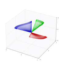
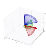
Figure 1. Examples of most probable paths on $\operatorname{SO}(3)$, illustrated by the action on the standard basis of $\mathbb{R}^{3}$ (red, green, blue vectors): (left) initial value problem of most probable path starting at the identity $e\in\operatorname{SO}(3)$ and evolving from initial conditions $\alpha_{0}$; (right) solution of boundary value problem of finding most probable paths between two points $e,g\in\operatorname{SO}(3)$.

In Figure 2, we find most probable path on the sphere $\mathbb{S}^{2}$ as projection of paths on the top space $\operatorname{SO}(3)$ of which $\mathbb{S}^{2}$ is a quotient. We set $\Sigma_{t}=\operatorname{id}_{3}$ but add non-trivial drift in the form of a vector field on $\mathbb{S}^{2}$. The field is horizontally lifted to $\operatorname{SO}(3)$ when solving the most probable paths equations (5.4). The figure shows the drift field, the solution of a boundary value problem and the corresponding paths on $\operatorname{SO}(3)$.

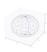
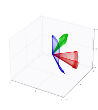
Figure 2. Examples of most probable paths on $\mathbb{S}^{2}$: (left) drift field $a$ on $\mathbb{S}^{2}$ (scaled arrows); (center) solution of boundary value problem of finding most probable paths between two points on $\mathbb{S}^{2}$; (right) path in $\operatorname{SO}(3)$ generating the most probable paths between the points on $\mathbb{S}^{2}$.

7.2. Landmark manifolds

We here illustrate most probable paths of diffeomorphisms acting on landmark configurations. We visualize the underlying deformations by their action on the initial landmark configuration for each $t$. The evolution is governed by equations of Theorem 6.3, given in coordinates in appendix A.3. Figure 3, left column shows the action on the landmark configuration of a most probable path of diffeomorphism, while, for comparison, Figure 3, right column shows most probable transformation between the same configurations following [11]. The results are shown for two different cases of noise fields (see figure caption). As discussed in remark 6.4, the most probable paths are paths of diffeomorphisms while the most probable transformations results in the flow lines of the landmarks being most probable.

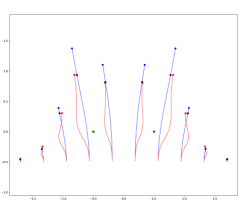
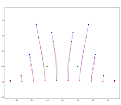
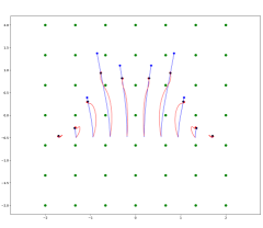
Figure 3. Most probable paths between two landmark configuration. Blue curves: trajectories wit no noise, only deterministic drift $a(t)$. Red curves: most probable paths to target configuration (black landmarks). Left column: most probable path as identified in Theorem 6.3. Right column: most probable transformation [11] that results in most probable flow lines. Noise fields $\sigma$ indicated by green dots. Top row: two noise fields. Botton row: 7x7 grid of noise fields.

In Figure 4, we perform the same experiments but now with configurations with 128 landmarks and $13\times 13$ grid of noise fields.

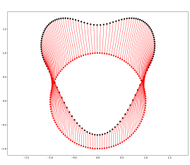
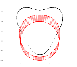
Figure 4. (left) most probable paths between two landmark configurations consisting of 128 points. (right) corresponding forward flow of the circle shape with no noise (only drift).

Appendix A Most probable paths in local coordinates

In all of the examples below, the manifold has dimension $d$ and summation over $d$ entries are in latin letters. We assume that the sub-Riemannian structure has rank $J$, and summation over $J$ entries are in greek letters.

A.1. General formulas for most probable paths

We want to give local description for the equation (3.1). Let $\gamma_{t}$ be a given curve starting at $o$. Let $(x^{1},\dots,x^{d})$ be a set of local coordinates on $M$ and define $x^{j}_{t}=x^{j}(\gamma_{t})$ and $u_{t}=\sum_{j=1}^{d}u^{j}_{t}\partial_{j}$. Write $\Gamma_{ij}^{k}$ for the Christoffel symbols of $\nabla$ in these coordinates, and write $T_{ij}^{k}$ and $R^{l}_{ijk}$ for local representation of respectively the torsion and the curvature. Let the sub-Riemannian structure $(E,g)$ have rank $J$. Choose a basis $f_{1,0},\dots,f_{d,0}$ of $T_{o}M$ such that $f_{1,0},\dots,f_{J,0}$ is an orthonormal basis of $E_{o}$. Write $\Sigma_{t}f_{\beta,0}=\sum_{\alpha=1}^{J}\Sigma_{\alpha\beta,t}f_{\alpha,0}$. Define $f_{1,t},\dots,f_{d,t}$ by parallel transport along $\gamma$. In other words, if we write $f_{r,t}=\sum_{j=1}^{d}f_{ir,t}\partial_{i}$, then they are solutions of

$$\dot{f}_{kr,t}=-\sum_{i,j,k=1}^{d}\dot{x}_{i}f_{jr,t}\Gamma_{ij}^{k}.$$

Let $f_{t}^{1},\dots,f_{t}^{d}$ be the corresponding coframe and write $f_{t}^{r}=\sum_{j=1}^{d}f^{rj}_{t}dx^{j}$, meaning that $(f_{t}^{ij})$ is the inverse matrix of $(f_{ij,t})$. Writing $\lambda_{t}=\sum_{i=1}^{d}\lambda_{i,t}f_{t}^{i}$ and $\chi_{t}=\frac{1}{2}\sum_{\alpha,\beta=1}^{J}\chi^{\alpha\beta}_{t}f_{\alpha,t}\wedge f_{\beta,t}$, then by evaluation of (3.1) along $f_{r,t}$, we obtain

$$\dot{\lambda}_{r,t} =-\sum_{i,k,l=1}^{d}\lambda_{l,t}f^{lk}_{t}f_{ir,t}\left(\partial_{i}u^{k}_{t}+\sum_{j=1}^{d}u_{t}^{j}\Gamma_{ij}^{k}+\sum_{j=1}^{d}\dot{x}_{j}T_{ij}^{k}\right)$$

$$\qquad+\sum_{i,j,k,l=1}^{d}\sum_{\alpha,\beta=1}^{J}\dot{x}_{i}\chi^{\alpha\beta}f_{jr,t}f_{k\alpha,t}f_{l\beta,t}R_{ijk}^{l},$$

$$\dot{\chi}_{t}^{\alpha\beta} =\frac{1}{2}\sum_{\nu=1}^{J}\lambda_{\nu,t}\left(\Sigma_{\alpha\nu,t}\lambda_{\beta,t}-\Sigma_{\beta\nu,t}\lambda_{\alpha,t}\right),\qquad\chi_{T}=0$$

$$\dot{x}_{t}^{k} =u_{t}^{k}+\sum_{\alpha,\beta=1}^{J}\Sigma_{\alpha\beta,t}\lambda_{\beta,t}f_{k\alpha,t}.$$

A.2. Most probable paths on Lie groups

We give a local description of the equations (4.2). We can solve the equation in the Lie algebra. Let $A_{1},\dots,A_{d}$ be a basis for $\mathfrak{g}$ such that $A_{1},\dots,A_{J}$ is an orthonormal basis of $\mathfrak{e}$. Write their Lie brackets as $[A_{i},A_{j}]=\sum_{k=1}c_{ij}^{k}A_{k}$. Write $\Sigma_{t}A_{\nu}=\sum_{\mu=1}^{J}\Sigma_{\mu\nu,t}$ and let $\alpha_{j,t}=\alpha_{t}(A_{j})$. Then most probable paths are solutions to equations

$$\left\{\begin{split}\dot{\alpha}_{j,t}&=-\sum_{k=1}^{d}\alpha_{k,t}\left(\sum_{\mu,\nu=1}^{J}\Sigma_{\mu\nu}\alpha_{\nu,t}c^{k}_{\mu j}+\sum_{i=1}^{d}a_{t}^{i}c_{ij}^{k}\right)\\ z_{t}&=\sum_{\mu,\nu=1}^{J}\Sigma_{\mu\nu}\alpha_{\mu,t}A_{\nu}+a_{t}\\ \dot{\gamma}&=z_{t}\cdot\gamma_{t}\end{split}\right.$$

A.3. Most probable paths for landmarks

We consider the equations for most probable paths for landmarks, described in Theorem 6.3 (b). We consider a curve $\boldsymbol{\gamma}_{t}=(\gamma_{1,t},\dots,\gamma_{n,t})$, and let $\lambda_{r,t}$ be a solution of (6.6). Let $(x^{1},\dots,x^{d})$ be the local coordinate system on $M$, and define

$$\lambda_{r,t}=\sum_{k=1}^{d}\lambda_{r,t}^{k}dx^{k},\qquad\sigma_{\alpha}=\sum_{k=1}^{d}\sigma_{\alpha}^{k}\partial_{k},\qquad a_{t}=\sum_{k=1}^{d}a_{t}^{k}\partial_{k},$$

and $x^{k}(\gamma_{r,t})=x_{r,t}^{k}$. Then we can solve

$$\dot{\lambda}_{r,t}^{k} =-\sum_{i=1}^{d}\sum_{\alpha=1}^{J}\lambda_{r,t}^{i}c_{\alpha,t}\partial_{k}\sigma_{\alpha}^{i}(\gamma_{r,t})-\sum_{i=1}^{d}\lambda_{r,t}^{i}\partial_{k}a_{t}^{i}(\gamma_{r,t}),$$

$$c_{\alpha,t} =\sum_{i,r=1}^{n}\lambda_{r,t}^{i}\sigma_{\alpha}^{i}(\gamma_{r,t}),$$

$$\dot{x}_{r,t}^{k} =a_{t}^{k}+\sum_{j=1}^{J}c_{\alpha,t}\sigma_{\alpha,t}^{k}(\gamma_{r,t}).$$

Appendix B Proof of Lemma 2.1 for absolutely continuous curves

We will give some details on an alternative proof of Lemma 2.1, which makes it more clear that it is still holds for absolutely continuous curves. In order to complete this, we need to define some additional structures on the general frame bundle not used other places of the paper. For proofs of these statements, see e.g. [11, Section 2.2 and 3.2].

Let $\operatorname{GL}(d)\to\operatorname{GL}(TM)\stackrel{{\scriptstyle\pi}}{{\to}}M$ be the general frame bundle over $M$. That is $\operatorname{GL}(TM)_{x}$ consist of all linear invertible maps $f=(f_{1},\dots,f_{n}):\mathbb{R}^{d}\to T_{x}M$, with $\operatorname{GL}(d)$ acting on the right by precomposition. For $f\in\operatorname{GL}(d)$, we define functions $\bar{T}:\operatorname{GL}(TM)\to\wedge^{2}(\mathbb{R}^{d})^{*}\otimes\mathbb{R}^{d}$ and $\bar{R}:\operatorname{GL}(TM)\to\wedge^{2}(\mathbb{R}^{d})^{*}\otimes(\mathbb{R}^{d})^{*}\otimes\mathbb{R}^{d}$ by $\bar{T}(f)=f^{-1}T(f\cdot,f\cdot)$ and $\bar{R}(f)=f^{-1}R(f\cdot,f\cdot)f$.

Consider $f_{t}=(f_{1,t},\dots,f_{d,t})$ as a $\nabla$-parallel frame along $\gamma_{t}$ with $f_{0}=f$ and $\dot{\gamma}_{0}=v$. Similar to Section 3.1, we define $\dot{f}_{t}|_{t=0}=h_{f_{0}}v$. We also write $H_{j}(f_{0})=h_{f_{0}}f_{j,0}$, giving us vector fields $H_{1},\dots,H_{d}$ on $\operatorname{GL}(TM)$. If $a=(a^{1},\dots,a^{d})\in\mathbb{R}^{d}$, we define $H_{a}=\sum_{i=1}^{d}a^{i}H_{i}$. Furthermore, for any $A\in\mathfrak{gl}(d)$, define a vector field $\xi_{A}$ by

$$\xi_{A}|_{f}=\frac{d}{dt}f\cdot e^{tA}|_{t=0}.$$

We then have Lie brackets $[H_{a},H_{b}]=-H_{\bar{T}(a,b)}-\xi_{\bar{R}(a,b)}$, $[\xi_{A},H_{a}]=H_{Aa}$ and $[\xi_{A},\xi_{B}]=\xi_{[A,B]}$. If we define one forms $\eta$ and $\theta$ with values in respectively $\mathfrak{gl}(d)$ and $\mathbb{R}^{d}$, by

$$\eta(\xi_{A}+H_{a})=A,\qquad\theta(\xi_{A}+H_{a})=a,$$

we then have relations $\Omega=d\eta+\frac{1}{2}[\eta,\eta]$ and $\Theta=d\theta+[\eta,\theta]$, where

$$\Omega(H_{a}+\xi_{A},H_{b}+\xi_{B})=\bar{R}(a,b),\qquad\Theta(H_{a}+\xi_{A},H_{b}+\xi_{B})=\bar{T}(a,b),$$

with $A,B\in\mathfrak{gl}(d),a,b\in\mathbb{R}^{d}$. This gives us the following result.

Lemma B.1.

Let $\omega,k\in\mathbb{H}^{T}(T_{o}M)$, then $\operatorname{Dev}(\omega+sk)$ is well defined and Lemma 2.1 holds.

Proof.

For $\omega,k\in\mathbb{H}^{T}(TM)$, then $\dot{\omega}+s\dot{k}_{t}$ is in $L^{2}$, and we can define $F:(-\varepsilon,\varepsilon)\times[0,T]\to\operatorname{GL}(M)$ as the solution of $F(s,0)=f_{0}\in\operatorname{GL}(TM)_{o}$ and

$$\partial_{t}F(s,t)=H_{f_{0}^{-1}(\dot{\omega}_{j,t}+s\dot{k}_{j,t})}(F(s,t))+hu_{t}(F(s,t)).$$

Write $f_{t}=F(0,t)$ and

$$\partial_{s}F(s,t)|_{s=0}=H_{f_{0}^{-1}v_{t}}+\xi_{f_{0}^{-1}A_{t}f_{0}}.$$

with $v_{t}$ and $A_{t}$ being curves in respectively $T_{o}M$ and $T^{*}_{o}M\otimes T_{o}M$ that vanish at time $t=0$. Then $\pi(F(t,s))=\gamma_{t}^{s}=\operatorname{Dev}_{u}(\omega+sk)_{t}$, $/\!/_{t}=f_{t}\circ f_{0}^{-1}$ and $\partial_{s}\gamma_{t}^{s}|_{s=0}=/\!/_{t}v_{t}$. We furthermore see that

$$(F^{*}\Omega)(\partial_{s},\partial_{t})|_{s=0}=\bar{R}_{f_{t}}(f_{t}^{-1}v_{t},f_{t}^{-1}(\dot{\omega}+u_{t,/\!/_{t}}))=f_{0}^{-1}R_{/\!/_{t}}(v_{t},\dot{\omega}+u_{t,/\!/_{t}})$$

$$=(F^{*}d\eta)(\partial_{s},\partial_{t})|_{s=0}+[(F^{*}\eta)(\partial_{s}),(F^{*}\eta)(\partial_{t})]|_{s=0}-[(F^{*}\eta)(\partial_{t}),F]$$

$$=-\partial_{t}F^{*}\eta(\partial_{s})|_{s=0}=-\partial_{t}f_{0}A_{t}f_{0}^{-1}$$

and

$$(F^{*}\Theta)(\partial_{s},\partial_{t})|_{s=0}=\bar{T}_{f_{t}}(f_{t}^{-1}v_{t},f_{t}^{-1}(\dot{\omega}+u_{t,/\!/_{t}}))$$

$$=f_{0}^{-1}T_{/\!/_{t}}(v_{t},\dot{\omega}+u_{t,/\!/_{t}})$$

$$=(F^{*}d\theta)(\partial_{s},\partial_{t})|_{s=0}+(F^{*}\eta)(\partial_{s})(F^{*}\theta)(\partial_{t})|_{s=0}$$

$$\qquad-(F^{*}\eta)(\partial_{t})(F^{*}\theta)(\partial_{s})|_{s=0}$$

$$=f_{0}^{-1}\dot{k}_{t}-f_{0}^{-1}\dot{v}_{t}+f_{0}^{-1}A_{t}(\dot{\omega}_{t}+u_{t,/\!/_{t}}).$$

It follows that we have equations $v_{0}=0$, $A_{0}=0$

$$\dot{A}_{t} =R_{/\!/_{t}}(\dot{\omega}+u_{t,/\!/_{t}},v_{t}),$$

$$\dot{k}_{t} =\dot{v}_{t}-T_{/\!/_{t}}(\dot{\omega}+u_{t,/\!/_{t}},v_{t})-A_{t}(\dot{\omega}_{t}+u_{t,/\!/_{t}}),$$

which is the statement of Lemma 2.1. ∎

References

- [1] A. Arnaudon, D. D. Holm, and S. Sommer. A Geometric Framework for Stochastic Shape Analysis. Foundations of Computational Mathematics, 19(3):653–701, June 2019.
- [2] M. Arnaudon, X. Chen, and A. B. Cruzeiro. Stochastic Euler-Poincaré reduction. J. Math. Phys., 55(8):081507, 17, 2014.
- [3] X. Bardina, C. Rovira, and S. Tindel. Onsager Machlup Functional for Stochastic Evolution Equations in a Class of Norms. Stochastic Analysis and Applications, 21(6):1231–1253, Jan. 2003.
- [4] U. Boscain and M. Sigalotti. Introduction to controllability of nonlinear systems. In Contemporary Research in Elliptic PDEs and Related Topics, pages 203–219. Springer, 2019.
- [5] M. Bruveris and F.-X. Vialard. On completeness of groups of diffeomorphisms. Journal of the European Mathematical Society, 19(5):1507–1544, 2017.
- [6] M. Capitaine. On the Onsager-Machlup functional for elliptic diffusion processes. Séminaire de probabilités de Strasbourg, 34:313–328, 2000.
- [7] L.-J. Cheng, E. Grong, and A. Thalmaier. Functional inequalities on path space of sub-Riemannian manifolds and applications. Nonlinear Anal., 210:Paper No. 112387, 30, 2021.
- [8] K. A. Coulibaly-Pasquier. Onsager-machlup functional for uniformly elliptic time-inhomogeneous diffusion. In Séminaire de Probabilités XLVI, pages 105–123. Springer, 2014.
- [9] A. Dembo and O. Zeitouni. Onsager-Machlup functionals and maximum a posteriori estimation for a class of non-gaussian random fields. Journal of Multivariate Analysis, 36(2):243–262, Feb. 1991.
- [10] T. Fujita and S.-i. Kotani. The Onsager-Machlup function for diffusion processes. Journal of Mathematics of Kyoto University, 22(1):115–130, 1982.
- [11] E. Grong and S. Sommer. Most probable flows for kunita sdes. arXiv preprint arXiv:2209.03868, 2022.
- [12] E. Grong and S. Sommer. Most probable paths for anisotropic Brownian motions on manifolds. accepted for Foundations of Computational Mathematics, arXiv:2110.15634, 2022.
- [13] K. Hara and Y. Takahashi. Lagrangian for pinned diffusion process. In N. Ikeda, S. Watanabe, M. Fukushima, and H. Kunita, editors, Itô’s Stochastic Calculus and Probability Theory, pages 117–128. Springer Japan, Tokyo, 1996.
- [14] H. Inci, T. Kappeler, and P. Topalov. On the regularity of the composition of diffeomorphisms. Mem. Amer. Math. Soc., 226(1062):vi+60, 2013.
- [15] H. Kunita. Stochastic Flows and Stochastic Differential Equations. Cambridge University Press, Apr. 1997.
- [16] S. Sommer and A. M. Svane. Modelling anisotropic covariance using stochastic development and sub-Riemannian frame bundle geometry. Journal of Geometric Mechanics, 9(3):391–410, June 2017.
- [17] Y. Takahashi and S. Watanabe. The probability functionals (Onsager-machlup functions) of diffusion processes. In D. Williams, editor, Stochastic Integrals, Lecture Notes in Mathematics, pages 433–463, Berlin, Heidelberg, 1981. Springer.
- [18] S. Watanabe and N. Ikeda. Stochastic Differential Equations and Diffusion Processes, Volume 24. North Holland, Amsterdam ; New York : Tokyo : New York, NY, Feb. 1981.
- [19] L. Younes. Shapes and Diffeomorphisms. Springer, 2010.