A Faster -means++ Algorithm
-means++ is an important algorithm for choosing initial cluster centers for the -means clustering algorithm. In this work, we present a new algorithm that can solve the -means++ problem with nearly optimal running time. Given data points in , the current state-of-the-art algorithm runs in iterations, and each iteration takes time. The overall running time is thus . We propose a new algorithm FastKmeans++ that only takes in time, in total.
1 Introduction
-means clustering aims to cluster data points from into clusters, such that the average distance between a data point and the center of the cluster it belongs to is minimized. -means has many important real-world applications in signal processing [28, 21] and unsupervised machine learning [19, 16].
A central problem in -means is how to pick the initial locations of the clusters to avoid -means from finding poor clusters. Much work focuses on finding a “good” initialization for the -means algorithm. The well-known heuristic Lloyd algorithm [42] performs well in practice while there is no theoretical guarantee for its approximation at initialization. There are already constant approximation algorithms with theoretical guarantee [39, 40]. Unfortunately, -approximation algorithm for arbitrary small does not exist if and can be large [44]. In recent works [7, 9, 10, 25], one achieved approximation algorithm. However, the running time of these algorithms depends on double exponentially. For fixed and , one may reduce input size or number of potential solutions to achieve constant approximation [34, 33, 24, 13, 41].
-means++ [4] is an algorithm that can find a center set that achieves approximation for the optimal center set. -means++ has thus been integrated into many standard machine learning libraries and is used as the default initialization method, replacing the traditional random initialization method. If allowed to sample centers, [1] shows that -means++ achieves constant bi-criteria approximation with constant probability. The more accurate trade-off between the number of centers to be sampled and the expected cost can be found in [56]. [3] provides a ratio approximation guarantee using primal-dual algorithm.
We note that applying a local search algorithm is one feasible way to achieve constant approximation for -means clustering [40, 26, 9, 25]. However, these algorithms suffer from a potentially large number of iterations. A more efficient -means++ algorithm via local search was proposed in [43] to achieve constant approximation. It is an iterative method that requires iterations, and each iteration has to take time. The overall running time is thus . This running time is fine for small and low-dimensional data, but it is increasingly insufficient for today’s explosion of dataset sizes , data dimensionality , and the number of clusters .
In this paper, we propose a faster version of the -means++ algorithm, called FastKMeans++. We show that choosing initial cluster locations can be much faster for constant approximation. We observe that the major computation cost originates from distance calculation. To accelerate the algorithm, especially for high dimensional situations, we design a distance oracle using JL lemmas [35] to approximate distance. We can approximate the -means++ algorithm in time and maintain constant approximation. When , we obtain optimal running time. In experiments, we use the -means++ algorithm [43] and FastKMeans++ algorithm to cluster the same synthetic point set respectively. We use -means++ as a baseline to evaluate the performance of FastKMeans++. Our experimental results demonstrate that FastKMeans++ is faster than -means++ in practice.
1.1 Our Results
We state an informal version of our results as follows.
Theorem 1.1 (Informal Version of Theorem 5.1).
Given point set and , the running time of Algorithm 3 is which uses space.
We use to denote the result of Algorithm 3. Let be the set of optimum centers. Then we have
Our result shows that our algorithm using a distance oracle still achieves constant approximation in expectation and runs in nearly optimal running time.
2 Related Work
Clustering
In [34], they showed the existence of small coresets for the problems of computing -means clustering for points in low dimensions. In [33], when they got clusterings for many different values of k, they used a quality measure of clusterings that is independent of k to determine a good choice of k, like the average silhouette coefficient. In [24], they use a weak (, k)-coreset to obtain a PTAS for the -means clustering problem with running time . In [13], they use coresets whose size is with polynomial dependency on the dimension d to maintain a -approximate -means clustering of a stream of points in . In [41], they provide simple randomized algorithms for the -means that yield approximations with probability and running times of . In [43], they provide a -approximation algorithm and runs in time. In [11], they provide a -approximation and runs in time. Our algorithm achieves -approximation and runs in . The approximation factor of [43] is the same as ours, but their running time is always slower than ours. The approximation factor of [11] is much worse than ours. Also when , their algorithm [11] takes while ours takes only .
Sketching for Iterative Algorithm
Sketching is an effective method to increase the speed of machine learning algorithms and optimization techniques. It involves compressing the large input matrix down to a much smaller sketching matrix that retains most of the key features of the original. As the algorithm now processes this smaller representation rather than the full high-dimensional input, its runtime can be substantially reduced. The core benefit is that the key information is preserved while removing redundant data that would otherwise slow computations. By working with this concise sketch version, large performance gains are possible without significantly impacting output quality.
In this work, we apply the sketching technique to an iterative algorithm. It is well-known that the sketching technique can be applied to many fundamental problems that are solved by the iterative type of algorithm. For example, linear programming [15, 38, 48, 29], empirical risk minimization [45, 47], cutting plane method [36], computing John Ellipsoid [12, 49], low-rank approximation [50], tensor decomposition [23], integral minimization problem [37], federated learning [6], linear regression problem [17, 46, 51, 53], matrix completion [32], training over-parameterized neural tangent kernel regression [5, 54, 58, 2], attention computation problem [52, 30, 31], and matrix sensing [20].
Roadmap
In Section 3, we introduce preliminary knowledge including notation and folklore lemmas. In Section 4, we present our data structure of DistanceOracle. In Section 5, we present the main results for FastKMeans++ algorithm. In Section 6, we demonstrate the running time and space storage for the algorithm. We provide the pseudocode of our algorithms and use a series of experiments to justify the advantages of our FastKMeans++ algorithm in Section 7. In Section 8, we draw our conclusion.
3 Preliminary
In Section 3.1, we first introduce several basic notations, such as the number of elements in a set, the distance between two nodes, and mathematical expectation. We introduce related definitions throughout the paper in Section 3.2, such as the sum of the distance between each node and its closest center and the mass center of multiple points. We present useful lemmas in Section 3.3, such as the method to calculate or estimate the sum of the distance between each node in a point set and a specific center or between a given node and each node in a center point set.
3.1 Notation
We use to denote set . Given finite set , we use to denote the number of elements in set . We use to denote norm in Euclidean space. We use to denote absolute value. Given random variable , we use to denote its expectation. For any function , we use to denote .
3.2 Related Definitions
We define the cost given data set and center set .
Definition 3.1 (Cost).
Given set and set , we define
Also, we define the mean or center of gravity for a point set.
Definition 3.2 (Mean).
Given data set , we define the mean of this set
3.3 Useful Lemmas
The following JL Lemma provides guidance for achieving distance oracle data structure.
Lemma 3.3 (JL Lemma, [35]).
For any of size , there exists an embedding where such that
Lemma 3.4.
Let be a point set. Let be a center. Let be defined as (Definition 3.2). Then we have
We present a variation of Corollary 21 in [27] which gives an upper bound on the cost difference.
Lemma 3.5.
For arbitrary , let be two different points in and be the center set. Then
4 Data Structure
In Section 4.1, we present the data structure of DistanceOracle. In Section 4.2, we state the running time results for DistanceOracle.
4.1 Distance Oracle
In this section, we state the result for the Distance Oracle data structure. In Init procedure, we preprocess the original data set using JL transform and store the transformed sketches. When we need to compute distance, we only use these sketches so that we can get rid of factor . We also use index set to denote current centers. We maintain a balanced search tree array of size that records the closet center for each data point and supports Insert, Delete, and GetMin operations. Using tree array , we are able to compute the current cost (Definition 3.1) with Cost operation and also the cost after adding a center with Query operation.
Theorem 4.1 (Distance Oracle).
There is a data structure that uses space
with the following procedures:
-
•
Init Given data , center , precision parameter and failure probability , it takes time to initialize.
-
•
Cost It returns an approximate cost using time such that
-
•
Insert Given index , it inserts distances between and all sketches to using time.
-
•
Delete Given index , it deletes all distances between and all sketches using time
-
•
Sample It samples an index using time
-
•
Query Given an index , it returns a value that satisfies
using time
Proof.
By Lemma 4.2, Lemma 4.3, Lemma 4.4, Lemma 4.5, Lemma 4.6 and Lemma 4.7, we obtain the running time for procedure Init, Cost, Insert, Delete, Sample and Query, respectively. In each of these lemmas, we calculate and prove the time complexity of each procedure.
In DistancOracle, it stores data points in , sketches in and maintain an -array. Each entry of the -array is a balanced search tree with nodes. Also, we have . The total space storage is
∎
4.2 Running Time of Distance Oracle
We start to prove the running time for Init.
Lemma 4.2 (Running Time of Init).
Given data , index set , precision parameter and failure probability , procedure Init takes time to initialize.
Proof.
Next, we turn to prove the running time for Cost.
Lemma 4.3 (Running Time of Cost).
Procedure Cost returns the current cost using time.
Proof.
We show the running time of Insert in the following lemmas.
Lemma 4.4 (Running Time of Insert).
Given index , it inserts distances between and all sketches to using time.
Proof.
We turn to prove the running time of Delete.
Lemma 4.5 (Running Time of Delete).
Given index , procedure Delete deletes all distances between and all sketches using time
Proof.
We present the running time of Sample
Lemma 4.6 (Running Time of Sample).
Procedure Sample samples an index according to probability using time.
Proof.
We show the running time of Query procedure.
Lemma 4.7 (Running Time of Query).
Given an index , procedure Query returns the sum of distances between and all sketches using time
5 Main Result
We state the main result for our algorithm including running time, space storage, and constant approximation guarantee.
Theorem 5.1 (Formal Version of Theorem 1.1).
Given data set , number of centers , precision parameter , failure probability and set , the running time of the FastKMeans++ algorithm is
Let be the output of our FastKMeans++ Algorithm 3. Let be the set of optimal centers. Then, we have
In addition this algorithm requires space.
6 Running Time and Space
Section 6.1 presents the running time for FastKMeans++ algorithm. Section 6.2 shows the running time for LocalSearch++. Section 6.3 states the space storage for FastKMeans++.
6.1 Running Time of FastKMeans++
In this section, we present the running time of the FastKMeans++ algorithm.
Lemma 6.1 (Running Time of FastKMeans++, Running tme of Theorem 5.1).
Given data set , number of cluster centers , precision , failure probability and , the running time of Algorithm 3 is
Proof.
The running time consists of three parts.
- •
- •
- •
Thus, the total running time for FastKMeans++ is
where the first step follows from , and the last step follows from summing all terms in the first step.
Thus, we complete the proof. ∎
6.2 Running Time of LocalSearch++
In this section, we prove the running time for LocalSearch++ (Algorithm 4)
Lemma 6.2 (Running Time of LocalSearch++).
Given data set and center set , the running time of LocalSearch++ is .
Proof.
In Line 3, it calls Sample procedure which takes time. Line 6 takes time. Line 7 is a for-loop with iterations. In each iteration, it takes time to run Delete (Line 8), to run Query procedure (Line 9) and to run Insert (Line 14). The running time for one step iteration is . Line 16 and Line 17 runs in time.
Thus, the total running time for LocalSearch++ is
Thus, we complete the proof. ∎
6.3 Space Storage
In this section, we prove the space storage of FastKMeans++ algorithm.
Lemma 6.3 (Space Storage For Algorithm 3, Space part of Theorem 5.1).
The space storage of Algorithm 3 is .
Proof.
We have the total space storage for FastKMeans++
Thus, we complete the proof. ∎
7 Experiments
Purpose. In this section, we use -means++ algorithm in [43] and FastKMeans++ algorithm in Theorem 5.1 to cluster the same synthetic point set respectively. We use -means++ as a baseline to evaluate the performance of FastKMeans++. We designed a new data structure DistanceOracle in Theorem 4.1. In DistanceOracle, we use a balanced search tree to store the nodes of each cluster to make the searching process faster. In order to shorten the time of calculating the distance between two nodes, we also create a sketching matrix that decreases the number of dimensions of each node. We adjust the parameters of our FastKMeans++ and original -means++ algorithm spontaneously to observe the influence of each parameter on their running time. Our summary of the result is as follows:
-
•
Our FastKMeans++ algorithm is much faster than original -means++ algorithm if is small enough.
-
•
The running time of -means++ and FastKMeans++ algorithm will increase linearly as increases.
-
•
The running time of original -means++ algorithm will increase linearly as increases, but doesn’t affect the running time of our FastKMeans++ algorithm very much.
-
•
The running time of our FastKMeans++ algorithm will increase linearly as increases, but is unrelated with the running time of original -means++ algorithm.
-
•
The running time of -means++ and FastKMeans++ algorithm will increase squarely as increases.
Setup. We use a computer of which the CPU is AMD Ryzen 7 4800H, GPU is RTX 2060 laptop. The operating system is Windows 11 Pro and we use Python as the code language. Let denote distance weights. Let denote the number of points in the point set. Let denote the dimension of each node. Let denote the dimension of each node after we process them with a sketching matrix. Let denote the number of clusters and centers. Let denote the number of iterations.
| Dataset Names | ||||
|---|---|---|---|---|
| SCADI | ||||
| MUPCI | ||||
| LM | ||||
| STDW |
Sythetic Data Generation. We generate random nodes of and each node is generated as follows
-
•
Pick each coordinate of node from .
-
•
Normalize each vector so that its norm is .
In the original -means++ algorithm, for node and node , we use to denote the distance between them. This takes time. As per update, it will take time since there are clusters containing points. For iterations, it takes time.
In our FastKMeans++ algorithm, we compute for . It takes time since there are nodes in total. So when we initialize our data structure, it will take time. In per update, we use to denote the distance between them. This takes time. So it will take time since we need to iterate over all clusters and calculate the distance to all other clusters.
For iterations, it will take time during the update process. Therefore, it will take
time in total.
Parameter Setting. In our experiments, we choose , , and as primary condition.
Real Datasets. In this part, we run -means++ and our FastKMeans++ algorithm on real data sets from UCI library [18] to observe if our algorithm is better than the original one in a real-world setting.
- •
-
•
Mturk User-Perceived Clusters over Images Data set [14]: This dataset random sampled images from the NUS-WIDE image database. Each image has features consisting of a bag of words based on SIFT descriptions.
-
•
Libras Movement Data set [22]: The dataset contains classes of instances each. In the video pre-processing, a time normalization is carried out selecting 45 frames from each video, according to a uniform distribution. In each frame, the centroid pixels of the segmented objects (the hand) are found, which compose the discrete version of the curve F with points. Each instance contains features of this curve F.
-
•
Sales Transactions Dataset Weekly Data set [55]: This data set contains sales transactions weekly. Each record has one product code and data for weeks.
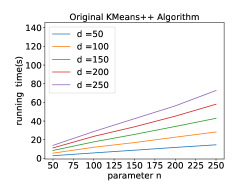
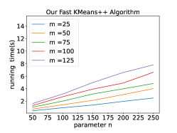
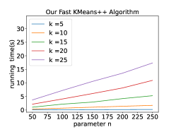
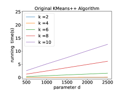
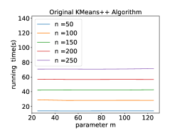
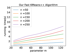
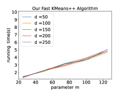
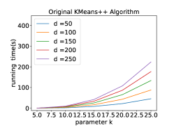
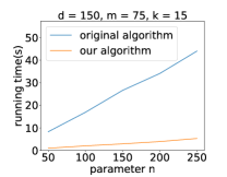
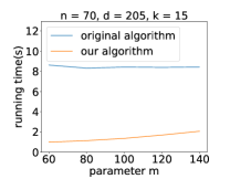
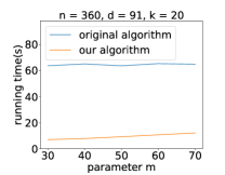
Results. To evaluate the influence of , we vary the value of while keeping other parameters the same. Fig. 1a indicates the running time of original -means++ and our FastKMeans++ algorithm increases linearly while increases. We note that our FastKMeans++ algorithm is faster than the original -means++ algorithm while changes. The ratio of the running time of the original -means++ to that of FastKMeans++ also increases from to as increases.
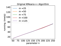
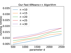
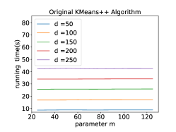
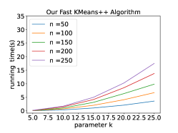
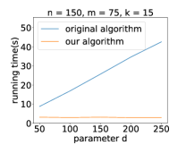
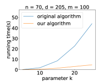
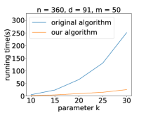
Then we estimate the influence of , we vary the value of while making sure during the whole testing process. We compare the performance of the original -means++ algorithm and our FastKMeans++ algorithm in Fig. 1b. It shows the running time of the original -means++ algorithm increases linearly while increases. The ratio of the running time of the original -means++ to that of FastKMeans++ also increases from to as increases. The running time of our FastKMeans++ seems unrelated with because in this case, is too small compared with other parameters like and . To show the influence of on our FastKMeans++ algorithm more clearly, we will explain it with more figures in the appendix.
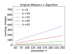
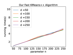
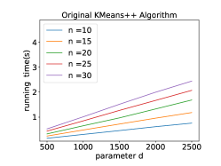
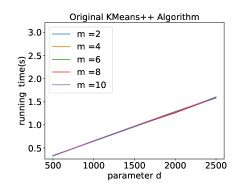
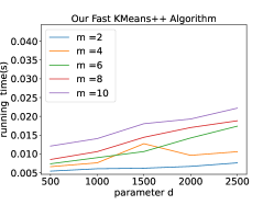
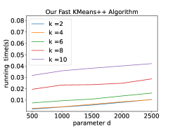
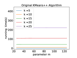
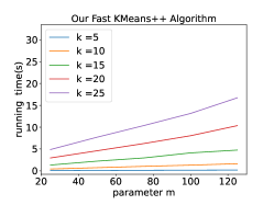
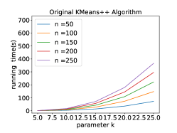
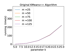
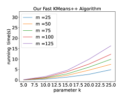
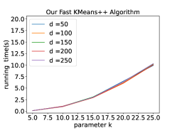
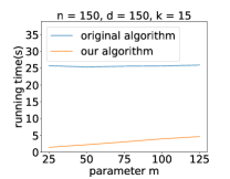
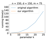
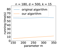
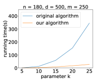
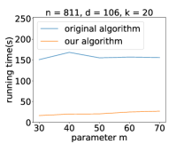
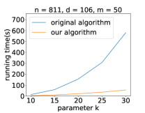
To evaluate the influence of , we vary the value of while keeping other parameters the same. Fig. 1c shows the running time of the original -means++ algorithm doesn’t change but that of our algorithm increases linearly while increases. And our FastKMeans++ algorithm runs faster compared to the original algorithm if is small enough. The ratio of the running time of the original -means++ to that of FastKMeans++ decreases from to as increases. We vary the value of and run -means++ and FastKMeans++. From Fig. 1d we can see that the running time of original -means++ and our algorithm increases squarely while increases. We note that our FastKMeans++ algorithm is faster than the original -means++ algorithm while changes. The ratio of the running time of the original -means++ to that of FastKMeans++ also increases from to as increases. This is consistent with our original thought.
Results for real data set. Fig. 2a, Fig. 2b, Fig. 3a and Fig. 3b show the relationship between the running time of -means++ algorithm and FastKmeans++ and parameter and on SCADI, MUPCI, Libras Movement and STDW data sets respectively. They show that our FastKmeans++ is much faster than the original -means++ algorithm on real data sets.
8 Conclusion
In this paper, we accelerate the -means++ algorithm using a distance oracle. We carefully design the data structure to support initialize, query, cost, etc. operations. We remove the factor of running time in each iteration of the local search. Finally, we run our FastKMeans++ algorithm and the original -means++ algorithm. In addition, we also implement our algorithm and obtain the experimental results which support our theoretical result. In this paper, we primarily focus on designing data structures and algorithms. We believe that proving a certain lower bound for our problem is also an interesting future direction. Our proposed FastKMeans++ algorithm not only improves computational efficiency but also maintains the quality of the clustering solution. We believe that our contributions will significantly advance the current state of scalable machine learning methods, opening up new possibilities for handling large-scale datasets.
Impact Statement
In this paper, we present the algorithm, theoretical analysis, and experiment. To the best of our knowledge, we do not foresee any potential negative societal consequences of our work.
References
- ADK [09] Ankit Aggarwal, Amit Deshpande, and Ravi Kannan. Adaptive sampling for k-means clustering. In Approximation, Randomization, and Combinatorial Optimization. Algorithms and Techniques, pages 15–28. Springer, 2009.
- ALS+ [22] Josh Alman, Jiehao Liang, Zhao Song, Ruizhe Zhang, and Danyang Zhuo. Bypass exponential time preprocessing: Fast neural network training via weight-data correlation preprocessing. arXiv preprint arXiv:2211.14227, 2022.
- ANFSW [19] Sara Ahmadian, Ashkan Norouzi-Fard, Ola Svensson, and Justin Ward. Better guarantees for k-means and euclidean k-median by primal-dual algorithms. SIAM Journal on Computing, 49(4):FOCS17–97, 2019.
- AV [06] David Arthur and Sergei Vassilvitskii. k-means++: The advantages of careful seeding. Technical report, Stanford, 2006.
- BPSW [21] Jan van den Brand, Binghui Peng, Zhao Song, and Omri Weinstein. Training (overparametrized) neural networks in near-linear time. In ITCS, 2021.
- BSY [23] Song Bian, Zhao Song, and Junze Yin. Federated empirical risk minimization via second-order method. arXiv preprint arXiv:2305.17482, 2023.
- BV [15] Sayan Bandyapadhyay and Kasturi Varadarajan. On variants of k-means clustering. arXiv preprint arXiv:1512.02985, 2015.
- BZ [19] SMM Fatemi Bushehri and Mohsen Sardari Zarchi. An expert model for self-care problems classification using probabilistic neural network and feature selection approach. Applied Soft Computing, 82:105545, 2019.
- CA [18] Vincent Cohen-Addad. A fast approximation scheme for low-dimensional k-means. In Proceedings of the Twenty-Ninth Annual ACM-SIAM Symposium on Discrete Algorithms, pages 430–440. SIAM, 2018.
- CAKM [19] Vincent Cohen-Addad, Philip N Klein, and Claire Mathieu. Local search yields approximation schemes for k-means and k-median in euclidean and minor-free metrics. SIAM Journal on Computing, 48(2):644–667, 2019.
- CALNF+ [20] Vincent Cohen-Addad, Silvio Lattanzi, Ashkan Norouzi-Fard, Christian Sohler, and Ola Svensson. Fast and accurate -means++ via rejection sampling. Advances in Neural Information Processing Systems, 33:16235–16245, 2020.
- CCLY [19] Michael B Cohen, Ben Cousins, Yin Tat Lee, and Xin Yang. A near-optimal algorithm for approximating the john ellipsoid. In Conference on Learning Theory, pages 849–873. PMLR, 2019.
- Che [09] Ke Chen. On coresets for k-median and k-means clustering in metric and euclidean spaces and their applications. SIAM Journal on Computing, 39(3):923–947, 2009.
- CLg+ [16] Ting-Yu Cheng, Guiguan Lin, xinyang gong, Kang-Jun Liu, and Shan-Hung (Brandon) Wu. Learning user perceived clusters with feature-level supervision. In D. Lee, M. Sugiyama, U. Luxburg, I. Guyon, and R. Garnett, editors, Advances in Neural Information Processing Systems, volume 29. Curran Associates, Inc., 2016.
- CLS [19] Michael B Cohen, Yin Tat Lee, and Zhao Song. Solving linear programs in the current matrix multiplication time. In STOC, 2019.
- CN [12] Adam Coates and Andrew Y Ng. Learning feature representations with k-means. In Neural networks: Tricks of the trade, pages 561–580. Springer, 2012.
- CW [13] Kenneth L Clarkson and David P Woodruff. Low-rank approximation and regression in input sparsity time. In Journal of the ACM (JACM), A Preliminary version of this paper is appeared at STOC, 2013.
- DG [17] Dheeru Dua and Casey Graff. UCI machine learning repository, 2017.
- DH [04] Chris Ding and Xiaofeng He. K-means clustering via principal component analysis. In Proceedings of the twenty-first international conference on Machine learning, page 29, 2004.
- DLS [23] Yichuan Deng, Zhihang Li, and Zhao Song. An improved sample complexity for rank-1 matrix sensing. arXiv preprint arXiv:2303.06895, 2023.
- DMC [15] Nameirakpam Dhanachandra, Khumanthem Manglem, and Yambem Jina Chanu. Image segmentation using k-means clustering algorithm and subtractive clustering algorithm. Procedia Computer Science, 54:764–771, 2015.
- DMR+ [09] Daniel B Dias, Renata CB Madeo, Thiago Rocha, Helton H Biscaro, and Sarajane M Peres. Hand movement recognition for brazilian sign language: a study using distance-based neural networks. In 2009 international joint conference on neural networks, pages 697–704. IEEE, 2009.
- DSY [23] Yichuan Deng, Zhao Song, and Junze Yin. Faster robust tensor power method for arbitrary order. arXiv preprint arXiv:2306.00406, 2023.
- FMS [07] Dan Feldman, Morteza Monemizadeh, and Christian Sohler. A ptas for k-means clustering based on weak coresets. In Proceedings of the twenty-third annual symposium on Computational geometry, pages 11–18, 2007.
- FRS [19] Zachary Friggstad, Mohsen Rezapour, and Mohammad R Salavatipour. Local search yields a ptas for k-means in doubling metrics. SIAM Journal on Computing, 48(2):452–480, 2019.
- FS [08] Gereon Frahling and Christian Sohler. A fast k-means implementation using coresets. International Journal of Computational Geometry & Applications, 18(06):605–625, 2008.
- FSS [20] Dan Feldman, Melanie Schmidt, and Christian Sohler. Turning big data into tiny data: Constant-size coresets for k-means, pca, and projective clustering. SIAM Journal on Computing, 49(3):601–657, 2020.
- GG [12] Allen Gersho and Robert M Gray. Vector quantization and signal compression, volume 159. Springer Science & Business Media, 2012.
- GS [22] Yuzhou Gu and Zhao Song. A faster small treewidth sdp solver. arXiv preprint arXiv:2211.06033, 2022.
- GSWY [23] Yeqi Gao, Zhao Song, Weixin Wang, and Junze Yin. A fast optimization view: Reformulating single layer attention in llm based on tensor and svm trick, and solving it in matrix multiplication time. arXiv preprint arXiv:2309.07418, 2023.
- GSY [23] Yeqi Gao, Zhao Song, and Junze Yin. An iterative algorithm for rescaled hyperbolic functions regression. arXiv preprint arXiv:2305.00660, 2023.
- GSYZ [23] Yuzhou Gu, Zhao Song, Junze Yin, and Lichen Zhang. Low rank matrix completion via robust alternating minimization in nearly linear time. arXiv preprint arXiv:2302.11068, 2023.
- HPK [05] Sariel Har-Peled and Akash Kushal. Smaller coresets for k-median and k-means clustering. In Proceedings of the twenty-first annual symposium on Computational geometry, pages 126–134, 2005.
- HPM [04] Sariel Har-Peled and Soham Mazumdar. On coresets for k-means and k-median clustering. In Proceedings of the thirty-sixth annual ACM symposium on Theory of computing, pages 291–300, 2004.
- JL [84] William B Johnson and Joram Lindenstrauss. Extensions of lipschitz mappings into a hilbert space. Contemporary mathematics, 26(189-206):1, 1984.
- JLSW [20] Haotian Jiang, Yin Tat Lee, Zhao Song, and Sam Chiu-wai Wong. An improved cutting plane method for convex optimization, convex-concave games and its applications. In STOC, 2020.
- JLSZ [23] Haotian Jiang, Yin Tat Lee, Zhao Song, and Lichen Zhang. Convex minimization with integer minima in time. arXiv preprint arXiv:2304.03426, 2023.
- JSWZ [21] Shunhua Jiang, Zhao Song, Omri Weinstein, and Hengjie Zhang. Faster dynamic matrix inverse for faster lps. In STOC, 2021.
- JV [01] Kamal Jain and Vijay V Vazirani. Approximation algorithms for metric facility location and k-median problems using the primal-dual schema and lagrangian relaxation. Journal of the ACM (JACM), 48(2):274–296, 2001.
- KMN+ [04] Tapas Kanungo, David M Mount, Nathan S Netanyahu, Christine D Piatko, Ruth Silverman, and Angela Y Wu. A local search approximation algorithm for k-means clustering. Computational Geometry, 28(2-3):89–112, 2004.
- KSS [10] Amit Kumar, Yogish Sabharwal, and Sandeep Sen. Linear-time approximation schemes for clustering problems in any dimensions. Journal of the ACM (JACM), 57(2):1–32, 2010.
- Llo [82] Stuart Lloyd. Least squares quantization in pcm. IEEE transactions on information theory, 28(2):129–137, 1982.
- LS [19] Silvio Lattanzi and Christian Sohler. A better k-means++ algorithm via local search. In International Conference on Machine Learning, pages 3662–3671. PMLR, 2019.
- LSW [17] Euiwoong Lee, Melanie Schmidt, and John Wright. Improved and simplified inapproximability for k-means. Information Processing Letters, 120:40–43, 2017.
- LSZ [19] Yin Tat Lee, Zhao Song, and Qiuyi Zhang. Solving empirical risk minimization in the current matrix multiplication time. In Conference on Learning Theory (COLT), pages 2140–2157. PMLR, 2019.
- NN [13] Jelani Nelson and Huy L Nguyên. Osnap: Faster numerical linear algebra algorithms via sparser subspace embeddings. In 2013 ieee 54th annual symposium on foundations of computer science, pages 117–126. IEEE, 2013.
- QSZZ [23] Lianke Qin, Zhao Song, Lichen Zhang, and Danyang Zhuo. An online and unified algorithm for projection matrix vector multiplication with application to empirical risk minimization. In AISTATS, 2023.
- SY [21] Zhao Song and Zheng Yu. Oblivious sketching-based central path method for linear programming. In International Conference on Machine Learning, pages 9835–9847. PMLR, 2021.
- SYYZ [22] Zhao Song, Xin Yang, Yuanyuan Yang, and Tianyi Zhou. Faster algorithm for structured john ellipsoid computation. arXiv preprint arXiv:2211.14407, 2022.
- [50] Zhao Song, Mingquan Ye, Junze Yin, and Lichen Zhang. Efficient alternating minimization with applications to weighted low rank approximation. arXiv preprint arXiv:2306.04169, 2023.
- [51] Zhao Song, Mingquan Ye, Junze Yin, and Lichen Zhang. A nearly-optimal bound for fast regression with guarantee. In International Conference on Machine Learning, pages 32463–32482. PMLR, 2023.
- [52] Zhao Song, Junze Yin, and Lichen Zhang. Solving attention kernel regression problem via pre-conditioner. arXiv preprint arXiv:2308.14304, 2023.
- [53] Zhao Song, Junze Yin, and Ruizhe Zhang. Revisiting quantum algorithms for linear regressions: Quadratic speedups without data-dependent parameters. arXiv preprint arXiv:2311.14823, 2023.
- SZZ [21] Zhao Song, Lichen Zhang, and Ruizhe Zhang. Training multi-layer over-parametrized neural network in subquadratic time. arXiv preprint arXiv:2112.07628, 2021.
- TSL [14] Swee Chuan Tan and Jess Pei San Lau. Time series clustering: A superior alternative for market basket analysis. In Proceedings of the First International Conference on Advanced Data and Information Engineering (DaEng-2013), pages 241–248. Springer, Singapore, 2014.
- Wei [16] Dennis Wei. A constant-factor bi-criteria approximation guarantee for k-means++. Advances in Neural Information Processing Systems, 29, 2016.
- ZBD [18] MS Zarchi, SMM Fatemi Bushehri, and M Dehghanizadeh. Scadi: A standard dataset for self-care problems classification of children with physical and motor disability. International Journal of Medical Informatics, 2018.
- Zha [22] Lichen Zhang. Speeding up optimizations via data structures: Faster search, sample and maintenance. Master’s thesis, Carnegie Mellon University, 2022.
Appendix
Roadmap.
Appendix A Correctness
In Section A.1, we defined two operations capture and reassign respectively. Then in Section A.2, we prove the upper bound for reassign operation. In Section A.3, we defined a good cluster whose index is in . is the subset of center set that capture (Definition A.1) exactly one cluster center from optimal center set . Then we calculate a lower bound for the proportion of good clusters under certain conditions. In Section A.4, we calculate a lower bound for the cost related to the mean center(Definition 3.2). In Section A.5, similar to Section A.3, we provide a definition of a good cluster for general cases. And we calculate a lower bound for the proportion of such good clusters under certain conditions. With lemmas and definitions in these sections, we prove that in each iteration of LocalSearch++, we can reduce the cost by with constant probability in Section A.6. Then in Section A.7, we prove the correctness of FastKMeans++.
A.1 Capture and Assign
In this section, we introduce two operations capture and assign.
Definition A.1 (Capture).
Let be optimal centers and is current cluster centers. An optimal center is captured by a center if
Then, we state the definition of reassign operation as follows.
Definition A.2 (Reassign).
Let be a data set. Let be cluster centers set and be the optimal cluster centers set. Let be the corresponding clusters. Let denote the subset of center set that capture (Definition A.1) exactly one cluster center from . Let be the subset of cluster centers that doesn’t capture (Definition A.1) any optimal centers. We use to denote the cluster with index and use to denote the cluster in captured by . We use a similar notation for the index .
For , we define the reassignment cost of as
For we define the reassignment cost of as
A.2 Upper Bound for Reassign Operation
In this section, we calculate an upper bound for reassign operation.
Lemma A.3.
For we have
Proof.
If a center does not capture any optimal center, we call it a lonely center. If a center is lonely, we think of it as a center that can be moved to a different cluster. We use to denote points obtained from by moving each point in , to . By Lemma 3.5 with , we obtain an upper bound for the change of cost with respect to , which results from moving the points to . For , we use to denote the point of to which has been moved. We have:
Taking all points in into consideration,
| (1) |
Note that all points from have been assigned to centers from . We turn to analyze the cost of moving the points back to the original location while maintaining the assignment. We use to denote the points in nearest to center and to represent the set of their original locations. For that was moved to , we have:
Taking all points in and the corresponding points in into consideration,
| (2) |
where the first step follows , the second step follows from Eq. (A.2) and the last step follows from .
Hence,
where the first step follows from definition of reassign and , the second step follows from inserting and the last step follows from Eq. (A.2) and Eq. (A.2).
∎
A.3 Good Cluster
In this section, we introduce the definition of ”good” for an index in (Definition A.2).
Definition A.4.
We define a good cluster index to be the one satisfying
The following lemma shows a lower bound for the proportion of good clusters under condition .
Lemma A.5.
Let be a constant. If , then
A.4 Lower Bound for Cost
In this section, the following lemma provides a lower bound for the cost related to the mean center (Definition 3.2)
Lemma A.6.
Given point set , center set of size and parameter . Let be the subset of such that from . If , we have
Proof.
Lemma 3.4 implies that the closest center in to has squared distance at least . Hence, the squared distance of points in to is at least
where we use that so that . By taking average, we get . With the inequality above we obtain the result. ∎
A.5 Good Cluster for General Cluster
In this section, we introduce definition of ”good” for general cluster index.
Definition A.7.
Let be the subset of cluster centers that doesn’t capture (Definition A.1) any optimal centers. For a general cluster index , we say it is good if there exists a center such that
We prove a lower bound similar to Lemma A.5 in the case .
Lemma A.8.
Let denote a constant. If and we have
Proof.
We already have . Note that . By the definition of good (Definition A.7) and Lemma A.3
where the first step follows from Definition A.7, the second step follows from and the last step follows from Lemma A.3.
Using , we obtain that
The bound follows from combining the previous inequality with ∎
A.6 Cost Reduction
Now, we can prove Lemma A.9. It suffices to show that using DistanceOracle, we can control the sampling error and give a constant lower bound for sampling probability.
Lemma A.9.
Let denote a constant. Let be a point set in . Let center set satisfying . Let . With probability , we have .
Proof.
Let be the set defined in Lemma A.6. For the case , we conclude that
where the first step follows from Lemma A.5 and Lemma A.6, the second step follows from Cost part of Theorem 4.1 and the last step follows from when ,with probability at least , .
With probability , we obtain lower bound . Conditioned on this event happening, we have probability at least to ensure the following analysis. The whole probability is . Thus, we can sample a point from with probability no less than .
By Definition A.4, when we sample a point in , we can replace it with to get an upper bound on the cost.
which follows from Definition A.4.
By Lemma 3.4 we have . Thus, with probability at least , we have
For the case , Lemma A.8 gives a similar lower bound as Lemma A.5. Using a similar technique as above, we conclude the same result for this case.
Thus, we complete the proof.
∎
A.7 Correctness of FastKMeans++
In this section, we show the correctness of our FastKMeans++ algorithm using Lemma A.9. We remark that as long as we prove Lemma A.9, then we can achieve the following result
Lemma A.10 (Correctness of FastKMeans++, correctness part of Theorem 5.1 ).
Given input data set , we set and use to denote the outcome of Algorithm 3. Let be the set of optimum centers. Then we have
Proof.
Let be a constant.
Let be the output of the first for-loop in Algorithm 3. Let be the final output of Algorithm 3. By Lemma A.9, conditioned on the fact that the cost of the centers is bigger than before the first call of LocalSearch++, we reduce the cost by a multiplicative factor with probability .
We construct an auxiliary random process to model the evolution of our algorithm. It starts with initial value . Then, it goes through iterations and reduces its value by a multiplicative factor with probability per iteration.
At the end of the process, it increases its value by adding quantity .
We note that the value of after iterations stochastically dominates the cost of the clustering. Thus, we have
where the first step follows from the expectation of binomial distribution, the second step follows from combining and and the last step follows from when .
This implies that . In the meanwhile,
| (3) |
where the first step follows from the definition of conditional expectation, the second step follows from Eq. (A.7) and the last step follows from .
Now the theorem follows from the following results in [4]
Hence,
∎
Appendix B More Experiments
Here we provide the links for the four real datasets.
-
•
SCADI Data Set [57, 8] 111https://archive.ics.uci.edu/ml/datasets/SCADI
-
•
Mturk User-Perceived Clusters over Images Data set [14]222https://archive.ics.uci.edu/ml/datasets/Mturk+User-Perceived+Clusters+over+Images
-
•
Libras Movement Data set [22]333https://archive.ics.uci.edu/ml/datasets/Libras+Movement
-
•
Sales Transactions Dataset Weekly Data set [55]444https://archive.ics.uci.edu/ml/datasets/Sales_Transactions_Dataset_Weekly
Let be the number of points in the point set. Let denote the dimension of each node. We use to denote the dimension of each node after we process them with a sketching matrix. Let be the number of clusters and centers. We provide more results of experiments to show the influence of , , , and in this part.
To evaluate if the influence of parameter will be affected by other parameters, we set different values for other parameters and run the original -means++ algorithm and our FastKMeans++ algorithm. Fig. 4 and Fig. 5 show that the running time of original -means++ and FastKMeans++ increase linearly as increases no matter what the value of other parameters is.
To evaluate if the influence of parameter will be affected by other parameters, we set different values for other parameters and run the original -means++ algorithm and our FastKMeans++ algorithm. To make the influence of on our FastKMeans++ more clear, I set large enough compared with , , and . Fig. 6 and Fig. 7 show that the running time of original -means++ and FastKMeans++ increase linearly as increases no matter what the value of other parameters is.
To evaluate if the influence of parameter will be affected by other parameters, we set different values for other parameters and run the original -means++ algorithm and our FastKMeans++ algorithm. Fig. 8 shows that is irrelevant to the running time of the original -means++ algorithm. Fig. 9 shows that the running time of FastKMeans++ increases linearly as increases no matter what the value of other parameters is.
To evaluate if the influence of parameter will be affected by other parameters, we set different values for other parameters and run the original -means++ algorithm and our FastKMeans++ algorithm. Fig. 10 and Fig. 11 show that the running time of original -means++ and FastKMeans++ increase squarely as increases no matter what the value of other parameters is.
When should we use FastKMeans++ algorithm? The result above demonstrates that our FastKMeans++ algorithm much faster than original -means++ algorithm. It also shows that if we set smaller, the running time of our algorithms will decrease too. Our FastKMeans++ algorithm behaves better compared with original -means++ algorithm especially when is very large. Therefore, our FastKMeans++ algorithm can handle the -means problem with high dimensional points.