Normalizing flows as an avenue to study overlapping gravitational wave signals

Abstract

Due to its speed after training, machine learning is often envisaged as a solution to a manifold of the issues faced in gravitational-wave astronomy. Demonstrations have been given for various applications in gravitational-wave data analysis. In this work, we focus on a challenging problem faced by third-generation detectors: parameter inference for overlapping signals. Due to the high detection rate and increased duration of the signals, they will start to overlap, possibly making traditional parameter inference techniques difficult to use. Here, we show a proof-of-concept application of normalizing flows to perform parameter estimation on overlapped binary black hole systems.

I Introduction

Over the last few years, the improved sensitivity of the LIGO Collaboration (2015) and Virgo Acernese et al. (2015) detectors has made the detection of gravitational waves (GWs) originating from compact binary coalescences (CBCs) more and more common, with over 90 detections reported after the third observation run Abbott et al. (2021a). This new information channel has had major impact in fundamental physics Abbott et al. (2021b), astrophysics Abbott et al. (2021c), and cosmology Abbott et al. (2021d). Soon, the upgrade of the current detectors and the addition of KAGRA Somiya (2012); Aso et al. (2013); Akutsu et al. (2019, 2020, 2021) and LIGO India Iyer et al. (2011) to the network of ground-based interferometers will lead to even more detections. In addition, the passage from second-generation (2G) to third-generation (3G) detectors (Einstein Telescope (ET) Punturo et al. (2010); Hild et al. (2011) and Cosmic Explorer (CE) Reitze et al. (2019); Abbott et al. (2017); Regimbau et al. (2017)) will lead to an important increase in the number of observed CBCs. These detectors are also projected to have a reduced lower frequency cutoff Sathyaprakash et al. (2012), leading to a longer duration for the signals. Therefore, CBC signals will likely overlap in 3G detectors Regimbau and Hughes (2009); Samajdar et al. (2021); Pizzati et al. (2022); Relton and Raymond (2021); Himemoto et al. (2021).

It has been established that analyzing one of the overlapping signals without accounting for the presence of the other can lead to biases in the recovered posteriors, especially when the merger times of the two events are close Samajdar et al. (2021); Pizzati et al. (2022); Relton and Raymond (2021); Himemoto et al. (2021); Antonelli et al. (2021). These could impact any direct science case for CBCs (e.g. tests of general relativity Wu and Nitz (2022)), but also indirectly related ones such as the hunt for primordial black holes, where subtraction of the foreground sources is required Sachdev et al. (2020); Sharma and Harms (2020); Biscoveanu et al. (2020); Zhou et al. (2022a, b); Reali et al. (2022). In Ref. Janquart et al. (2022), the authors demonstrate on two overlapped binary black holes (BBHs) how using adapted Bayesian inference can help reduce the biases. They use two methods: (i) hierarchical subtraction, where one analyzes the dominant signal first and subtracts it before analyzing the second event, and (ii) joint parameter estimation, where the two signals are analyzed jointly. They show that the second method is less prone to biases, but computationally heavier. Their analysis also suffers some instabilities, and further upgrades are needed for it to be entirely reliable. An issue also mentioned in this work is the computational time. Indeed, more than $10^{5}$ CBC mergers are expected in the 3G era Samajdar et al. (2021). So having analyses taking several weeks to complete is not a realistic alternative.

While it is true that traditional methods can be sped-up Zackay et al. (2018); Dai et al. (2018); Leslie et al. (2021); Morisaki (2021), or that quantum computing Gao et al. (2022) could potentially be used in the future, the development of frameworks capable of doing complete analyses in very short timescales is crucial for the development of 3G detectors. Therefore, in this work, we propose the first step in that direction, showing how overlapping BBHs can be analyzed with machine learning, and more specifically, a normalizing flow Jimenez Rezende and Mohamed (2015); Kingma et al. (2016); Papamakarios et al. (2017) approach. We start by presenting our machine-learning model. Then we show the setup of our analysis and the results obtained. Finally, we give our conclusions and outline some prospects.

II Machine learning for overlapping gravitational waves

The use of machine learning in GW data analysis has been growing over the last years, having a wide range of applications. See Ref. Cuoco et al. (2021) for a review. A subset of these methods fall under the umbrella of simulation-based inference Cranmer et al. (2020), and are being developed to perform parameter estimation for CBCs Delaunoy et al. (2020); Green et al. (2020); Green and Gair (2021); Dax et al. (2021a, b, 2022); Williams et al. (2021). Dax et al. (2021a, b, 2022) use normalizing flows to get posterior distributions for BBH parameters. Such methods have been shown to have results close to those from MCMC and nested sampling. Our approach is somewhat similar to theirs, with some notable differences explained below.

Our approach uses continuous conditional normalizing flows Kobyzev et al. (2021); Papamakarios et al. (2019), which is a variant of normalizing flows suited for probabilistic modeling and Bayesian inference problems. Due to the recursive and continuous nature of these models their memory footprint can be quite small Chen et al. (2018). These qualities allow for extensive training on home-grade GPUs while retaining the ability to capture complex distributions. We cover them in more detail below.

Normalizing flows are a method in machine learning through which a neural network can learn the mapping from some simple base distribution $p_{u}(\boldsymbol{u})$ (a Gaussian, for example) to a more complex final distribution $q(\boldsymbol{\theta})$. This is done through a series of invertible and differentiable transformations, summarized by a function $g(\boldsymbol{\theta})$. However, in our case, it is not sufficient to go from one distribution to the other. We also need to do this conditionally on the GW data that we wish to analyze. To account for this, we use conditional normalizing flows Winkler et al. (2019), where the transformation functions are dependent on the data $\boldsymbol{d}$ (hence, $g=g(\boldsymbol{\theta},\boldsymbol{d})$). A major difference with Winkler et al. (2019) is that our base distributions are kept static; experiments on toymodels did not show any benefits in having conditional priors. Thus our model $g(\boldsymbol{\theta},\boldsymbol{d})$ is a trainable conditional bijective function that transforms a simple 30-D Gaussian into a 30-D complex distribution. The bijectivity allows us to express and sample $q(\boldsymbol{\theta}|\boldsymbol{d})$ in terms of $g(\boldsymbol{\theta},\boldsymbol{d})$ and $p_{u}(\boldsymbol{u})$ via the change of variable theorem:

$$q(\boldsymbol{\theta}|\boldsymbol{d})=\big{|}\rm{det}(J_{g^{-1}}(\boldsymbol{\theta},\boldsymbol{d}))\big{|}p_{u}(g^{-1}(\boldsymbol{\theta},\boldsymbol{d}))\,,$$ (1)

where $\rm{det}(J_{g^{-1}}(\boldsymbol{\theta},\boldsymbol{d}))$ is the determinant of the Jacobian $J_{g^{-1}}(\boldsymbol{\theta},\boldsymbol{d})$ of the transformation. We train the model by minimizing the forward KL-divergence, which is equivalent to maximum likelihood estimation Papamakarios et al. (2017); Papamakarios and Murray (2016). As noted by Dax et al. (2022), $q(\boldsymbol{\theta}|\boldsymbol{d})$ should cover the actual (Bayesian) posterior $p(\boldsymbol{\theta}|\boldsymbol{d})$, and asymptotically approach it as training progresses due to the mode-covering nature of the forward KL divergence.

A distinctive choice of our method is the continuous nature of the flow, which is linked to the transformation function itself. Neural ordinary differential equations (neural ODEs)Chen et al. (2018) are the foundation of continuous normalizing flows; neural ODEs are not represented by a stack of discrete layers but a hypernetwork Ha et al. (2017). Hypernetworks can be understood as regular networks where ‘external’ inputs such as a (continuous) time or depth variable smoothly changes the output of the network for identical inputs. They can thus represent multiple networks or transformations. In Chen et al. (2018), hypernetworks are used to represent ODEs and are trained by using ODE-solvers and clever use of the adjoint sensitivity method. A continuous normalizing flow uses neural ODEs as it transformations.

We will now explain the training of a continuous flow. For clarity we will use $h$ to refer to a continuous transformation and $g$ for a discrete one. If $\boldsymbol{\theta}(t)$ represents the samples from the distribution at a given time $t$, when going from $t_{1}$ to $t_{2}$, the continuous normalizing flow obeys an ordinary differential equation

$$\frac{\rm{d}\boldsymbol{\theta}(t)}{\rm{d}t}=h(t,\boldsymbol{\theta}(t))\,.$$ (2)

The change in likelihood associated with this ‘step’ differs slightly from equations 1 due to the continuous nature of the flow:

$$\log(p(\boldsymbol{\theta}(t_{1})))=\log(p(\boldsymbol{\theta}(t_{0})))-\int_{t_{0}}^{t_{1}}\rm{Tr}\big{[}J_{g}(\boldsymbol{\theta}(t))\big{]}\,.$$ (3)

Assuming a non-stiff ODE the integration can be performed rapidly with state-of-the-art ode-solvers, which in our case is MALI Zhuang et al. (2021). In addition, we have to solve a trace instead of a determinant, which reduces the complexity, going from $\mathcal{O}(D^{3})$ to at most $\mathcal{O}(D^{2})$ with $D$ being the dimensionality of posterior space, and speed-ups the computation. Moreover, using continuous normalizing flows removes the need to use coupling layers between transformations, instead all parameter dimensions can be dependent on each other throughout the flow. Combining the continuous and conditional flows leads to continuous conditional normalizing flows, where the conditional consists of the GW $\boldsymbol{d}$ and the time $t$.

We also need a better data representation than the raw strain to train and analyze the data. Therefore, we follow a similar approach as in Green and Gair (2021); Green et al. (2020); Dax et al. (2021a, b, 2022), using a single value decomposition (SVD) Halko et al. (2009) as summary statistics, reducing the dimension and the noise content of the data. Each of the 256 generated basis vectors is used as a kernel in 1D convolutions used as an initial layer in a residual convolutional neural network (CNN), enabling one to capture the time variance of the signal. Therefore, we do not need to use a Gibbs sampler to estimate the time of the signal as is done in Dax et al. (2021a, b, 2022), and can sample over time like any other variable which allows us to retain the likelihood of the samples. Furthermore, we also use a different representation for the angles. Instead of directly using their values, we project them onto a sphere for the sky location and onto a circle for the other angles. This makes for a better-posed domain for these angles, plays on the strong interpolation capacities of the network, and makes the training step easier.

In the end, our framework combines data representation as a hybrid between classical SVD and CNN, followed by the continuous normalizing flow network. It is worth noting that our entire framework is relatively small compared to the ones presented in Dax et al. (2021a). It enables the network to run on lower-end GPUs, but also means the network could be limited in his capacity to model the problem.

III Data and setup

To test the capacity of our framework to deal with overlapping signals, we start with a simplified setup. We consider a network made of the two LIGO detectors and the Virgo detector, at design sensitivity Barsotti et al. (2021); Acernese et al. (2015), and with a lower sensitive frequency of $20$Hz. We generate Gaussian noise from their power spectral density (PSD) and inject two precessing BBH mergers generated with the IMRPhenomPv2 waveform Khan et al. (2016). Our data frames have an 8 seconds duration. The chirp mass ($\mathcal{M}_{c}=(M_{1}+M_{2})^{3/5}/(M_{1}M_{2})^{1/5}$) is sampled from a uniform distribution between 10$M_{\odot}$ and 100$M_{\odot}$, and the mass ratio ($q=M_{2}/M_{1}$) from a uniform distribution between 0.125 and 1. We constrain the individual component masses between 5$M_{\odot}$ and 100$M_{\odot}$. During the data generation, the luminosity distance is kept fixed. It is then rescaled to result in a network signal-to-noise ratio value taken randomly between 10 and 50, sampled from a beta distribution with central value 20. The time of coalescence for the two events is set randomly around a time of reference, with $t_{c}\in[t_{\rm{ref}}-0.05,t_{\rm{ref}}+0.05]$, ensuring that the two BBH merge in the high bias regime Pizzati et al. (2022). The other parameters are drawn from their usual domain. Table 1 gives an overview of the parameters and the function from which they are sampled.

Parameter	Function
Chirp mass	$\mathcal{U}(10,100)M_{\odot}$
Mass ratio	$\mathcal{U}(0.125,1)$
Component masses	Constrained in [5, 100]$M_{\odot}$
Luminosity distance	Rescaled to follow SNR
SNR	$\mathcal{B}(10,50)$
Coalescence time	$\mathcal{U}(t_{\rm{ref}}-0.05,t_{\rm{ref}}+0.05)$
Spin Amplitudes	$\mathcal{U}(0,1)$
Spin tilt angles	Uniform in sine
Spin vector azimuthal angle	$\mathcal{U}(0,2\pi)$
Spin precession angle	$\mathcal{U}(0,2\pi)$
Inclination angle	Uniform in sine
Wave polarization	$\mathcal{U}(0,\pi)$
Phase of coalescence	$\mathcal{U}(0,2\pi)$
Right ascension	$\mathcal{U}(0,2\pi)$
Declination	Uniform in cosine

Table 1: Summary of the parameters considered for the BBHs generated as well as the functions used for their generation.

During the training, we continuously generate the data by sampling the prior distributions for the events and generating a new noise realization for each data frame. The training is stopped when convergence is reached and before over-fitting occurs. Our model trained for about 12 days on a single Nvidia GeForce GTX 1080.

IV Results

First, we show the corner plots recovered for the masses and sky location of the two events in a pair in Fig. 1. These are representative of our results. One can see that the injected values are within the 90% confidence interval. This is the case for most events, regardless of the relative difference in arrival time or the SNR ratio between the two.

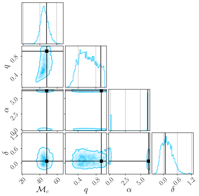
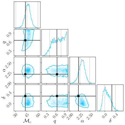
Figure 1: Example recovery for the masses and sky location of two overlapped BBHs with the machine learning approach. We see that the recovered values are well within the 90% confidence interval.

To demonstrate the method’s reliability, P-P plots for the two signals recovery are shown in Fig. 2. The P-P plot is constructed by sampling the posteriors of 1000 overlapped events. We then compute in which percentile of the distribution the injected value lies. If everything goes as expected the cumulative density functions should align along the diagonal. One can observe that this is the case for our network. Comparing this to the results given in Dax et al. (2021a) for single signals, there is a broadening of the shell around the diagonal, showing more variability in the signal recovery. This means that our inference is less accurate than for single signals. Possible origins are the degenerate posteriors, increased complexity of the problem, and the reduced size of our network. In addition, an increased variability has been noted when going from single parameter estimation to joint parameter estimation methods in Bayesian approaches Janquart et al. (2022).

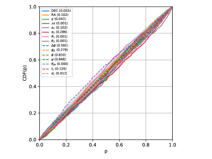
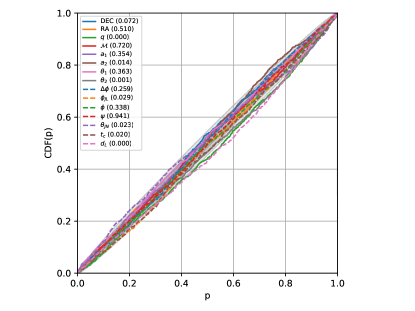
Figure 2: P-P plots for the recovered parameters for the two events in the data. In both cases, the lines align along the diagonal, showing that our method can be trusted. The larger spread can be due to bimodalities in the data, the increased complexity of the problem, and the reduced size of our network.

A trick used to alleviate the problem of degeneracies is to time-order the samples. Indeed, for two BBHs, the likelihood is symmetric in the two events. Therefore, the posteriors can get bimodal Janquart et al. (2022). While our training method formally labels one event as A and the other event as B, when the characteristics of the events are close, we may get somewhat bimodal posteriors. This probably also contributes to the higher variability of the P-P plot.

Since parameter estimation for overlapping signals is still an active field of research, it is difficult to compare with traditional methods. While methods have been developed in Janquart et al. (2022), they are not yet fully stable and take a long time to analyze a BBH system. Therefore, making a statistically significant study comparing the two approaches seems a bit premature at this stage. However, to have some sense of the performances of our network compared to traditional methods, we make 15 injections complying with our network’s setup and analyze them with the framework presented in Janquart et al. (2022). While this is not enough to make a statistical comparison, we can already identify some trends between the two pipelines. The first is that our machine pipeline typically has broader posteriors than the Bayesian approach. As mentioned in Ref. Janquart et al. (2022), the classical joint parameter estimation approach can sometimes get overconfident, where the recovered injected value lies outside of the 90% confidence interval. Our method is not confronted with this bottleneck as the broader posterior encapsulates the injected value. Fig. 3 represents the two situations: one where the Bayesian approach finds the event correctly, and one where we see that our ML approach covers the injected values while it does not for the classical approach. The origin of the larger posterior, which is not observed in the single parameter estimation machine learning-based methods, is probably due to the increased complexity of the problem combined with our network’s small size. One possible avenue is applying importance sampling after the normalizing flow Kolmus et al. (2022); Dax et al. (2022). This would increase the computational time, but the time needed to go from events to samples would still be well below the time taken by the traditional methods. However, such methods can be tricky, and additional modifications to our network could be needed.

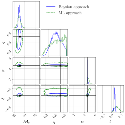
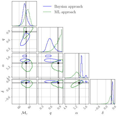
Figure 3: Comparison between our approach and the approach from Janquart et al. (2022). Our posteriors are generally broader but encapsulate the injected value within the 90% confidence interval. This could be corrected by applying importance sampling on the samples given by our network.

Finally, an important advantage of our method is its speed. After being trained, it can analyze two overlapping BBH signals in about a second, to compare with $\mathcal{O}(20days)$ reported in Janquart et al. (2022). While it is difficult to estimate the time gain for other types of signals, such as BNSs or NSBHs, we can expect the inference time after training not to be significantly larger than for BBHs. Since the computation time is a crucial aspect for studies in the 3G era, machine learning approaches seem to be more suited to study realistic scenarios for these detectors.

V Conclusions and Perspectives

In this work, we have presented a proof-of-concept machine learning-based method to analyze overlapping BBH signals. We focused on a 2G detector scenario with the two LIGO, and the Virgo detectors at design sensitivity, with a lower frequency cutoff of 20Hz. Our approach is based on continuous normalizing flows.

While also using normalizing flows, as in Green and Gair (2021); Green et al. (2020); Dax et al. (2021a, b, 2022), we bring extra modifications that seem to help in the inference task. We represent the data through a mixture of SVD and convolutions, enabling us to sample directly over the events’ arrival time, removing the need to use additional Gibbs sampling steps over that parameter and retaining the ability to access the likelihood of a sample. We also move to continuous conditional normalizing flows, reducing the computational cost of the method as we need to solve a trace instead of a determinant when going from one step to the other in the transformation. Finally, we also use a particular representation of the angles, projecting them onto circles (for the phase, the polarization, …) and spheres (for the sky location). We believe that these modifications make our network more supple, enabling it to deal with overlapping signals even in a reduced form.

With this simplified setup, we have shown that our approach is reliable, with posteriors consistent with the injected values. Our method takes about one week to train on a single GPU. After that, it only takes about a second to analyze two overlapped BBHs. While, in reality, other types of CBC mergers can happen, their inference after training should not be significantly longer than for BBHs. We also compared our machine learning method with classical Bayesian methods for overlapping signals. While our scheme leads to wider posteriors, it can correctly recover the injected values, even when the Baysian approach gets overconfident and misses the injection. A possibility to correct for the widened posteriors is to use importance sampling.

Our method’s combined reliability and speed show that machine learning is a viable approach to analyze CBC mergers in the 3G era. More interestingly, it would even be possible without needing to account for the development of more powerful computational means and could enable some science-case studies for ET and CE soon. For example, once trained for all possible BBH systems, it could help study the BBH mass function in the 3G era.

Still, one should note that extra improvements are needed before using our method in realistic 3G scenarios. One would first need to change our setup to the 3G detectors, a lower frequency and extreme SNRs that could be encountered. In addition, a wider range of objects should be accounted for. One should account for higher-order modes and eccentricity that could play a crucial role in the 3G era. Other modifications could also be implemented. Additionally, we need to account for the change in noise realization from one event to the other. Some of these steps, like changing the detectors, should be relatively easy. Others are more complex, as it is hard to perform parameter inference for long-lasting mergers due to the computational burden. So, extra developments in parameter estimation using machine learning would be required to get to the realistic 3G scenario. For overlapping signals, one would also benefit from developments in the classical study of the 3G scenario, such as how to deal with the noise characterization or the types of other events that could come into the data.

In the end, there is still work to be done before machine learning can be used in realistic 3G scenarios. However, we believe that this work shows it is an interesting avenue and could be practical on a relatively short time scale.

References

- Collaboration (2015) T. L. S. Collaboration, Classical and Quantum Gravity 32, 074001 (2015).
- Acernese et al. (2015) F. Acernese et al. (VIRGO), Class. Quant. Grav. 32, 024001 (2015), arXiv:1408.3978 [gr-qc] .
- Abbott et al. (2021a) R. Abbott et al. (LIGO Scientific, VIRGO, KAGRA), (2021a), arXiv:2111.03606 [gr-qc] .
- Abbott et al. (2021b) R. Abbott et al. (LIGO Scientific, VIRGO, KAGRA), (2021b), arXiv:2112.06861 [gr-qc] .
- Abbott et al. (2021c) R. Abbott et al. (LIGO Scientific, VIRGO, KAGRA), (2021c), arXiv:2111.03634 [astro-ph.HE] .
- Abbott et al. (2021d) R. Abbott et al. (LIGO Scientific, VIRGO, KAGRA), (2021d), arXiv:2111.03604 [astro-ph.CO] .
- Somiya (2012) K. Somiya (KAGRA), Class. Quant. Grav. 29, 124007 (2012), arXiv:1111.7185 [gr-qc] .
- Aso et al. (2013) Y. Aso, Y. Michimura, K. Somiya, M. Ando, O. Miyakawa, T. Sekiguchi, D. Tatsumi, and H. Yamamoto (KAGRA), Phys. Rev. D 88, 043007 (2013), arXiv:1306.6747 [gr-qc] .
- Akutsu et al. (2019) T. Akutsu et al. (KAGRA), Nature Astron. 3, 35 (2019), arXiv:1811.08079 [gr-qc] .
- Akutsu et al. (2020) T. Akutsu, M. Ando, K. Arai, et al., arXiv e-prints , arXiv:2005.05574 (2020), arXiv:2005.05574 [physics.ins-det] .
- Akutsu et al. (2021) T. Akutsu et al. (KAGRA), PTEP 2021, 05A101 (2021), arXiv:2005.05574 [physics.ins-det] .
- Iyer et al. (2011) B. Iyer, T. Souradeep, C. Unnikrishnan, S. Dhurandhar, S. Raja, and A. Sengupta, “LIGO-India Tech. rep. ,” https://dcc.ligo.org/LIGO-M1100296/public (2011).
- Punturo et al. (2010) M. Punturo et al., Classical and Quantum Gravity 27, 194002 (2010).
- Hild et al. (2011) S. Hild et al., Class. Quant. Grav. 28, 094013 (2011), arXiv:1012.0908 [gr-qc] .
- Reitze et al. (2019) D. Reitze et al., Bull. Am. Astron. Soc. 51, 035 (2019), arXiv:1907.04833 [astro-ph.IM] .
- Abbott et al. (2017) B. P. Abbott, R. Abbott, T. D. Abbott, M. R. Abernathy, K. Ackley, and C. Adams, Classical and Quantum Gravity 34, 044001 (2017).
- Regimbau et al. (2017) T. Regimbau, M. Evans, N. Christensen, E. Katsavounidis, B. Sathyaprakash, and S. Vitale, Phys. Rev. Lett. 118, 151105 (2017).
- Sathyaprakash et al. (2012) B. Sathyaprakash et al., Class. Quant. Grav. 29, 124013 (2012), [Erratum: Class.Quant.Grav. 30, 079501 (2013)], arXiv:1206.0331 [gr-qc] .
- Regimbau and Hughes (2009) T. Regimbau and S. A. Hughes, Phys. Rev. D 79, 062002 (2009), arXiv:0901.2958 [gr-qc] .
- Samajdar et al. (2021) A. Samajdar, J. Janquart, C. Van Den Broeck, and T. Dietrich, Phys. Rev. D 104, 044003 (2021), arXiv:2102.07544 [gr-qc] .
- Pizzati et al. (2022) E. Pizzati, S. Sachdev, A. Gupta, and B. Sathyaprakash, Phys. Rev. D 105, 104016 (2022), arXiv:2102.07692 [gr-qc] .
- Relton and Raymond (2021) P. Relton and V. Raymond, Phys. Rev. D 104, 084039 (2021), arXiv:2103.16225 [gr-qc] .
- Himemoto et al. (2021) Y. Himemoto, A. Nishizawa, and A. Taruya, Phys. Rev. D 104, 044010 (2021), arXiv:2103.14816 [gr-qc] .
- Antonelli et al. (2021) A. Antonelli, O. Burke, and J. R. Gair, Mon. Not. Roy. Astron. Soc. 507, 5069 (2021), arXiv:2104.01897 [gr-qc] .
- Wu and Nitz (2022) S. Wu and A. H. Nitz, (2022), arXiv:2209.03135 [astro-ph.IM] .
- Sachdev et al. (2020) S. Sachdev, T. Regimbau, and B. S. Sathyaprakash, Phys. Rev. D 102, 024051 (2020).
- Sharma and Harms (2020) A. Sharma and J. Harms, Phys. Rev. D 102, 063009 (2020).
- Biscoveanu et al. (2020) S. Biscoveanu, C. Talbot, E. Thrane, and R. Smith, Phys. Rev. Lett. 125, 241101 (2020).
- Zhou et al. (2022a) B. Zhou, L. Reali, E. Berti, M. Çalışkan, C. Creque-Sarbinowski, M. Kamionkowski, and B. S. Sathyaprakash, (2022a), arXiv:2209.01310 [gr-qc] .
- Zhou et al. (2022b) B. Zhou, L. Reali, E. Berti, M. Çalışkan, C. Creque-Sarbinowski, M. Kamionkowski, and B. S. Sathyaprakash, (2022b), arXiv:2209.01221 [gr-qc] .
- Reali et al. (2022) L. Reali, A. Antonelli, R. Cotesta, S. Borhanian, M. Çalışkan, E. Berti, and B. S. Sathyaprakash, (2022), arXiv:2209.13452 [gr-qc] .
- Janquart et al. (2022) J. Janquart, T. Baka, A. Samajdar, T. Dietrich, and C. Van Den Broeck, (2022), arXiv:2211.01304 [gr-qc] .
- Zackay et al. (2018) B. Zackay, L. Dai, and T. Venumadhav, (2018), arXiv:1806.08792 [astro-ph.IM] .
- Dai et al. (2018) L. Dai, T. Venumadhav, and B. Zackay, (2018), arXiv:1806.08793 [gr-qc] .
- Leslie et al. (2021) N. Leslie, L. Dai, and G. Pratten, Phys. Rev. D 104, 123030 (2021), arXiv:2109.09872 [astro-ph.IM] .
- Morisaki (2021) S. Morisaki, Phys. Rev. D 104, 044062 (2021), arXiv:2104.07813 [gr-qc] .
- Gao et al. (2022) S. Gao, F. Hayes, S. Croke, C. Messenger, and J. Veitch, Phys. Rev. Res. 4, 023006 (2022), arXiv:2109.01535 [quant-ph] .
- Jimenez Rezende and Mohamed (2015) D. Jimenez Rezende and S. Mohamed, arXiv e-prints , arXiv:1505.05770 (2015), arXiv:1505.05770 [stat.ML] .
- Kingma et al. (2016) D. P. Kingma, T. Salimans, R. Jozefowicz, X. Chen, I. Sutskever, and M. Welling, arXiv e-prints , arXiv:1606.04934 (2016), arXiv:1606.04934 [cs.LG] .
- Papamakarios et al. (2017) G. Papamakarios, T. Pavlakou, and I. Murray, arXiv e-prints , arXiv:1705.07057 (2017), arXiv:1705.07057 [stat.ML] .
- Cuoco et al. (2021) E. Cuoco et al., Mach. Learn. Sci. Tech. 2, 011002 (2021), arXiv:2005.03745 [astro-ph.HE] .
- Cranmer et al. (2020) K. Cranmer, J. Brehmer, and G. Louppe, Proceedings of the National Academy of Sciences 117, 30055 (2020).
- Delaunoy et al. (2020) A. Delaunoy, A. Wehenkel, T. Hinderer, S. Nissanke, C. Weniger, A. R. Williamson, and G. Louppe, (2020), arXiv:2010.12931 [astro-ph.IM] .
- Green et al. (2020) S. R. Green, C. Simpson, and J. Gair, Phys. Rev. D 102, 104057 (2020), arXiv:2002.07656 [astro-ph.IM] .
- Green and Gair (2021) S. R. Green and J. Gair, Mach. Learn. Sci. Tech. 2, 03LT01 (2021), arXiv:2008.03312 [astro-ph.IM] .
- Dax et al. (2021a) M. Dax, S. R. Green, J. Gair, M. Deistler, B. Schölkopf, and J. H. Macke, (2021a), arXiv:2111.13139 [cs.LG] .
- Dax et al. (2021b) M. Dax, S. R. Green, J. Gair, J. H. Macke, A. Buonanno, and B. Schölkopf, Phys. Rev. Lett. 127, 241103 (2021b), arXiv:2106.12594 [gr-qc] .
- Dax et al. (2022) M. Dax, S. R. Green, J. Gair, M. Pürrer, J. Wildberger, J. H. Macke, A. Buonanno, and B. Schölkopf, (2022), arXiv:2210.05686 [gr-qc] .
- Williams et al. (2021) M. J. Williams, J. Veitch, and C. Messenger, Phys. Rev. D 103, 103006 (2021), arXiv:2102.11056 [gr-qc] .
- Kobyzev et al. (2021) I. Kobyzev, S. J. Prince, and M. A. Brubaker, IEEE Transactions on Pattern Analysis and Machine Intelligence 43, 3964 (2021).
- Papamakarios et al. (2019) G. Papamakarios, E. Nalisnick, D. Jimenez Rezende, S. Mohamed, and B. Lakshminarayanan, arXiv e-prints , arXiv:1912.02762 (2019), arXiv:1912.02762 [stat.ML] .
- Chen et al. (2018) R. T. Chen, Y. Rubanova, J. Bettencourt, and D. K. Duvenaud, Advances in neural information processing systems 31 (2018).
- Winkler et al. (2019) C. Winkler, D. Worrall, E. Hoogeboom, and M. Welling, arXiv e-prints , arXiv:1912.00042 (2019), arXiv:1912.00042 [cs.LG] .
- Papamakarios and Murray (2016) G. Papamakarios and I. Murray, arXiv e-prints , arXiv:1605.06376 (2016), arXiv:1605.06376 [stat.ML] .
- Ha et al. (2017) D. Ha, A. M. Dai, and Q. V. Le, in International Conference on Learning Representations (2017).
- Zhuang et al. (2021) J. Zhuang, N. C. Dvornek, sekhar tatikonda, and J. s Duncan, in International Conference on Learning Representations (2021).
- Halko et al. (2009) N. Halko, P.-G. Martinsson, and J. A. Tropp, arXiv e-prints , arXiv:0909.4061 (2009), arXiv:0909.4061 [math.NA] .
- Barsotti et al. (2021) L. Barsotti, P. Fritschel, M. Evans, and S. Gras, “Advanced LIGO anticipated sensitivity curves,” https://dcc.ligo.org/LIGO-T1800044/public (2021).
- Khan et al. (2016) S. Khan, S. Husa, M. Hannam, F. Ohme, M. Pürrer, X. Jiménez Forteza, and A. Bohé, Phys. Rev. D 93, 044007 (2016), arXiv:1508.07253 [gr-qc] .
- Kolmus et al. (2022) A. Kolmus, G. Baltus, J. Janquart, T. van Laarhoven, S. Caudill, and T. Heskes, Phys. Rev. D 106, 023032 (2022), arXiv:2111.00833 [gr-qc] .