Hierarchical Proxy Modeling for Improved HPO
in Time Series Forecasting

Abstract.

Selecting the right set of hyperparameters is crucial in time series forecasting. The classical temporal cross-validation framework for hyperparameter optimization (HPO) often leads to poor test performance because of a possible mismatch between validation and test periods. To address this test-validation mismatch, we propose a novel technique, H-Pro to drive HPO via test proxies by exploiting data hierarchies often associated with time series datasets. Since higher-level aggregated time series often show less irregularity and better predictability as compared to the lowest-level time series which can be sparse and intermittent, we optimize the hyperparameters of the lowest-level base-forecaster by leveraging the proxy forecasts for the test period generated from the forecasters at higher levels. H-Pro  can be applied on any off-the-shelf machine learning model to perform HPO. We validate the efficacy of our technique with extensive empirical evaluation on five publicly available hierarchical forecasting datasets. Our approach outperforms existing state-of-the-art methods in Tourism, Wiki, and Traffic  datasets, and achieves competitive result in Tourism-L  dataset, without any model-specific enhancements. Moreover, our method outperforms the winning method of the M5  forecast accuracy competition.

1. Introduction

Time series data is often associated with a hierarchy. For example, in the retail domain, daily sales of a certain product in a store constitute a product-level time series. Aggregating all product-level time series in the store at each time point gives a cumulative store-level series consisting of the daily sales of that particular store. Similarly, aggregated time series can be obtained at other levels like department, state, and country (Makridakis et al., 2022). The notion of generating forecasts at every level of the data hierarchy is generally termed as “hierarchical time series forecasting” (Hyndman and Athanasopoulos, 2021), and it has been an active area of research in recent years (see Section 3). Hierarchical forecasting generally requires coherent forecasts at every level; i.e., the forecast at an aggregated level should be the exact sum of the forecasts of its children nodes in an associated hierarchy tree. Accurate and coherent forecasts at different levels of the hierarchy ensure that consistent and correct business decisions are taken at different parts of an organization.

(a) Temporal cross-validation

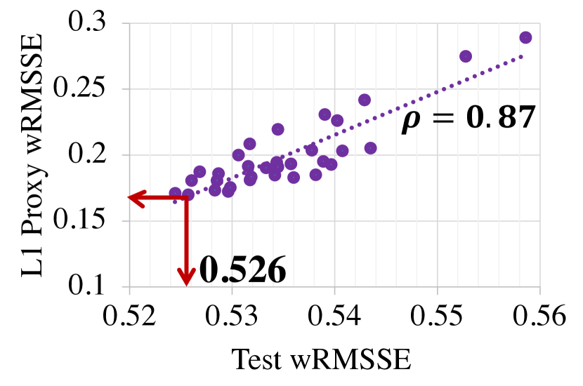
(b) Proposed H-Pro

Figure 1. Variation of test error with (a) validation, and (b) proxy errors in all HPO trials (dots) for a store-clustered LightGBM model on M5 data. (a): Lowest validation errors do not correspond to the lower range of test errors due to data mismatch. (b): The lowest proxy error often selects a model with better test error, and better linear fit is observed with higher correlation, $\rho$, between test and proxy errors.

A hierarchical forecasting algorithm consists of two components (either decoupled or integrated): a base-forecasting method, and a reconciliation technique that ensures coherent forecasts. Recently, complex machine learning (ML) models with a large number of hyperparameters are becoming popular in forecasting since they can learn from multiple time series and leverage the shared information between them, contrary to some of the classical forecasters like SARIMA, exponential smoothing, etc.  Examples include gradient boosting models like LightGBM (Makridakis et al., 2022), and DNN-based models like DeepAR (Salinas et al., 2020), N-BEATS (Oreshkin et al., 2020), and Informer (Zhou et al., 2021). This leads to an increase in the adoption of complex ML models for hierarchical forecasting as well due to their superior performance (Rangapuram et al., 2021; Paria et al., 2021; Das et al., 2022; Mancuso et al., 2021).

The performance of these models depends on hyperparameters that are generally tuned on validation window(s) via temporal cross-validation (TCV) (Hyndman and Athanasopoulos, 2021). TCV chronologically splits the historical time series data into train and validation windows. Thus, the validation windows often differ in characteristics from the test data. The mismatch between validation and test is prevalent in time series compared to other ML domains because of varying statistical properties of temporal data (Hyndman and Athanasopoulos, 2021; Akgiray, 1989). The problem is exacerbated in hierarchical forecasting because of higher data irregularity (and sometimes intermittency) at the lowest level. This can lead to suboptimal hyperparameter optimization (HPO) and poor model selection, particularly at the lowest level of the hierarchy (see Figure 1(a)).

We propose a novel HPO technique for hierarchical time series forecasting. It is based on the frequent observation that time series at the lowest level of the hierarchy are sparse, irregular, and sometimes intermittent in nature such as in (Makridakis et al., 2022). However, the aggregated series at higher levels are generally more consistent and have better predictability. Based on this observation, we develop H-Pro, a method for performing HPO of the lowest-level forecasting model based on one or more proxy forecaster(s) at higher levels. The proxy forecasters are trained on higher-level aggregated time series, and their forecasts for the test period are obtained. The lowest-level model treats these forecasts as proxies to the original time series for the test period, and the HPO of the lowest-level model is performed with respect to the higher-level proxy forecasts instead of validation windows as done in conventional TCV (Figure. 2). Thus, by effectively leveraging the better predictability of the aggregated series, the lowest-level models are regularized via HPO. The lowest-level forecasts are then aggregated bottom-up (Section 3) to derive higher-level forecasts leading to coherent and accurate forecasts at all levels. From Figure 1(b), we can see that H-Pro helps in model selection, i.e., choosing a model with the minimum proxy error criteria corresponds to a much better test error compared to conventional TCV.

1.0.1. Summary of contributions

(1) To address the commonly occurring test-validation mismatch issue in forecasting, we propose a novel technique, H-Pro that drives HPO via test proxies by exploiting the data hierarchy and better predictability of higher level forecasters. (2) To the best of our knowledge, this is the first work which empirically and theoretically demonstrate that we can obtain coherent and accurate hierarchical forecasts just by employing hierarchical proxy-guided HPO on off-the-shelf ML models. Specifically, H-Pro outperforms state-of-the-art results in Tourism, Traffic, and Wiki data, and achieves competitive result in Tourism-L  data. Moreover, H-Pro  outperforms the winning method of the M5  forecast accuracy competition. (3) State-of-the-art hierarchical reconciliation methods like MinT and ERM (Section 3) can be computationally expensive for datasets with large number of time series, but the proposed H-Pro does not suffer from this scalability issue. A detailed comparison is in Appendix A. (4) We also show in experiments that H-Pro helps improve the performance of TCV when ensembled with it, and hence, emphasize the complementary knowledge captured by the method.

2. Background and Notations

2.1. Forecasting

Let $x_{1:T}$ represent a univariate time series of length $T$, i.e., at any time-point $t$, $x_{t}\in\mathbb{R}$. The task of forecasting is to predict $H$ value(s) in the future given the history $x_{1:T}$,

(1) $$\hat{x}_{T+1:T+H}=f(x_{1:T})$$

where $f(\cdot)$ is the map learned by a forecasting algorithm $\mathcal{A}$, and $H$ is the forecast horizon. Here we focus on algorithms that learn a shared map $f$ for multiple related time series, as these often work best in practice (e.g., modern forecasting models like DeepAR, N-BEATS, and LightGBM).

2.2. Hierarchical forecasting

A hierarchical time series dataset is associated with a hierarchy tree that has $L$ levels ($l=1$ for the top level, and $l=L$ for the lowest level). We denote the set of levels by $[L]=\{1,\dots,L\}$, and the nodes at a level $l$ by $[N_{l}]=\{1,\dots,N_{l}\}$. The time series at the leaf nodes are called lowest-level series, and the time series at other nodes are called higher-level/aggregated series. The higher-level series at any node $j\in[N_{l}]$ of level $l\in[L-1]$ follows the coherence criteria (Hyndman and Athanasopoulos, 2021): $x_{t}^{l,j}=\sum_{i\in{C_{l,j}}}x^{(l+1),i}_{t}$, where $C_{l,j}$ is the set of children of node $j$ of level $l$. The task is to forecast accurately at all nodes of all levels so that the forecast at any higher-level node also follows the coherence constraint, i.e., $\hat{x}_{t}^{l,j}=\sum_{i\in{C_{l,j}}}\hat{x}^{(l+1),i}_{t},\forall l\in[L-1],j\in[N_{l}]$.

2.2.1. Hierarchical evaluation

Hierarchical forecasts are evaluated with a hierarchically aggregated metric that can indicate the average error across all levels (Makridakis et al., 2022). Generally, every level is given equal weight while aggregating the level-wise metrics, ensuring unbiased evaluation of hierarchical forecasts across all levels. Hence, any hierarchical forecasting technique should aim to attain accurate and coherent forecasting at all levels. More details will be provided in Section 5.

3. Related work

Classical methods of hierarchical forecasting rely on generating base forecasts for every time series, and reconcile them to produce coherent forecasts at every level. For example, the bottom-up (BU) approach produces lowest level forecasts, and simply aggregates them to obtain coherent forecasts at all levels (Hyndman and Athanasopoulos, 2021). Similarly, top-down and middle-out approaches take particular aggregate level forecasts and disaggregate them to lower levels (Hyndman and Athanasopoulos, 2021). The MinT  optimal reconciliation algorithm takes independent forecasts and produces coherent hierarchical forecasts by incorporating information from all levels simultaneously via a linear mapping to the base series (Wickramasuriya et al., 2019; Hyndman and Athanasopoulos, 2021). MinT minimizes the sum of variances of the forecast errors when the individual forecasts are unbiased. (Ben Taieb and Koo, 2019) relaxed the unbiasedness condition, and proposed ERM which optimizes the bias-variance trade-off by solving an empirical risk minimization problem. Since ERM  is a successor of MinT, we refer both of them as optimal reconciliation algorithms throughout the text. (Rangapuram et al., 2021) proposed HierE2E which trains a single neural network on all time series together. It enforces coherence conditions in model training. Another end-to-end approach was proposed in (Mancuso et al., 2021) where the reconciliation is imposed in a customized loss function of the neural network. A probabilistic top-down approach was proposed in (Das et al., 2022) where a distribution of proportions is learnt by an RNN model to split the parent forecast among its children nodes. A top-down alignment-based reconciliation was developed in (Anderer and Li, 2021) where the lowest-level forecasts are adjusted based on the higher-level forecasts. The method employs a bias-controlling multiplier for the loss function of the lowest-level model, optimized by manual grid search. We want to highlight that the proposed H-Pro is compatible with any search algorithm (see Section 5.2 for details). Moreover, AutoML frameworks like (Abdallah et al., 2022; Deng et al., 2023) can internally employ H-Pro for hierarchical forecasting tasks.

4. H-Pro

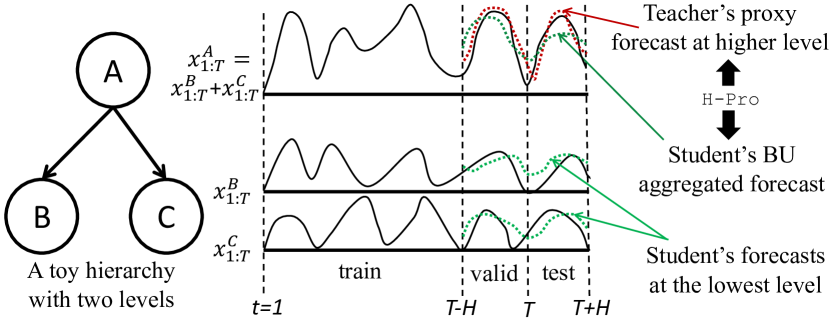
Figure 2. Visual explanation of H-Pro for a toy hierarchy. Temporal cross-validation performs HPO on the validation period with the actual ground truth data. H-Pro performs HPO on the test period with the teacher’s proxy forecast.

We derive the HPO objective for conventional TCV, and then, extend it for H-Pro. For both cases, the models are trained at the lowest level, but their HPO techniques differ. Bottom-up (BU) aggregation is employed in both scenarios to generate coherent forecasts. We denote a learning algorithm by $\mathcal{A}\left(\mathcal{X}^{L}_{\mathrm{train}};\lambda\right)$, where $\mathcal{X}^{L}_{\mathrm{train}}$ is the training data at the lowest level, $\lambda$ denotes the hyperparameters, and we ignore the model’s parameters since those are learned in a separate optimization regime (not our focus). The goal of HPO is to find the best $\lambda$ by minimizing an objective. For a given $\lambda$, $\mathcal{A}$ provides the forecasting map $f_{\lambda}$ as shown in (1). We subscript $f$ with $\lambda$ to concisely denote the forecasting model’s dependency on the algorithm’s hyperparameters.

4.1. HPO with temporal cross-validation (TCV)

Traditionally, TCV has been used to perform HPO and model selection for forecasting (Salinas et al., 2020; Oreshkin et al., 2020). Figure 2 shows the train, validation, and test splits for TCV with one validation window. Hence, those subsets can be expressed with time-ranges. For example, $\mathcal{X}^{L}_{\mathrm{train}}=\{x^{L,j}_{1:T-H}\}_{j=1}^{N_{L}}$, and so on. We show the HPO objectives below for one validation window, but it can be generalized to multiple windows as well. Irrespective of the number of validation windows, the model is trained again on the entire train and validation period (i.e., on $\mathcal{X}^{L}_{\mathrm{train+valid}}$) with the optimal hyperparameters $\lambda^{*}$ to produce test forecasts, $\hat{x}^{L,j}_{T+1:T+H}$.

The HPO for TCV can target either the lowest-level error, or a hierarchically aggregated error (see Section 2.2). We denote the two variants as TCV-Lowest and TCV-Hier. Following (Bergstra and Bengio, 2012), the HPO objective for a single-validation TCV-Lowest can be written as

$$\lambda^{\ast}_{\mathrm{TCV\emph{-}Lowest}}\approx\operatorname*{argmin}_{\lambda\in\Lambda}\operatorname*{mean}_{x^{L}\in\mathcal{X}^{L}_{\mathrm{valid}}}\left[\mathcal{L}\left(x^{L},\hat{x}^{L}\right)\right]$$

(2) $$=\operatorname*{argmin}_{\lambda\in\Lambda}\frac{1}{N_{L}}\sum_{j=1}^{N_{L}}\mathcal{L}\left(x^{L,j}_{T-H+1:T},f_{\lambda}\left(x^{L,j}_{1:T-H}\right)\right).$$

While TCV-Lowest  targets minimizing lowest-level error, TCV- Hier  better targets the hierarchical forecasting objective as it aims to obtain low error at all levels. Formally,

$$\lambda^{\ast}_{\mathrm{TCV\emph{-}Hier}}\approx\operatorname*{argmin}_{\lambda\in\Lambda}\frac{1}{L}\sum_{l=1}^{L}\biggl{[}\frac{1}{N_{l}}\times\biggl{.}$$

(3) $$\sum_{j=1}^{N_{l}}\left[\mathcal{L}\left(x^{l,j}_{T-H+1:T},\mathcal{B}\left(f_{\lambda},\left\{x^{L,i}_{1:T-H}\right\}_{i=1}^{N_{L}},l,j\right)\right)\right]\biggr{.}\biggr{]}$$

where, $\mathcal{B}\left(\cdot\right)$ is the bottom-up aggregation function which aggregates forecasts from the descendant leaf nodes to produce a forecast at node $j$ of level $l$.

4.2. HPO with hierarchical proxy modeling

From (4.1) and (4.1) we can see that $\lambda^{\ast}_{\mathrm{TCV\emph{-}Hier}}$ and $\lambda^{\ast}_{\mathrm{TCV\emph{-}Lowest}}$ depend on the validation data $x^{l,j}_{T-H+1:T}$. Hence, a mismatch between the test series $x^{l,j}_{T+1:T+H}$ and validation series $x^{l,j}_{T-H+1:T}$ can lead to poor test performance. H-Pro attempts to address the issue based on the observation that, often, the higher-level aggregated time series are less irregular and have better predictability (e.g., in (Makridakis et al., 2022)). It builds two sets of models: a student model as a base forecaster at the lowest level, and teacher model(s) as proxy forecasters at any (or all) higher levels (see Figure 2). The student produces the final forecasts at all levels via bottom-up (BU) aggregation.

H-Pro proceeds as follows. The teacher model(s) are trained and their HPO is performed with TCV. Teacher’s forecasts are generated for the test period. We term these as teacher’s proxy forecasts since the student treats them as the actual ground truth for the unknown test period. The student is trained on the entire train and validation data at the lowest level, but its HPO is performed based on the proxy forecasts at higher levels. Intuitively, the student model is regularized in a way such that it tries to mimic the proxy forecasts of the teacher, but only at higher level(s) since teacher’s forecasts are not available at the lowest level. We hypothesize that even if we guide the student to produce accurate forecasts at higher level(s) for the test period, it would enable the student to produce accurate forecasts in all or at least some of the lower levels because the higher level forecasts are obtained by aggregating the lower level forecasts (Figure. 2).

Following (4.1), the H-Pro objective can be written as

$$\lambda^{\ast}_{\texttt{H-Pro}}\approx\operatorname*{argmin}_{\lambda\in\Lambda}\sum_{l=1}^{L-1}\biggl{[}w(l)\cdot\frac{1}{N_{l}}\times\biggl{.}$$

(4) $$\sum_{j=1}^{N_{l}}\left[\mathcal{L}\left(\tilde{x}^{l,j}_{T+1:T+H},\mathcal{B}\left(f_{\lambda},\left\{x^{L,i}_{1:T}\right\}_{i=1}^{N_{L}},l,j\right)\right)\right]\biggr{.}\biggr{]}$$

where, $\tilde{x}^{l,j}_{T+1:T+H}$ denotes the teacher’s proxy forecasts at that node, and $w(l)\in[0,1]$ assigns a confidence-weight on the teacher at level $l$. Hence, $\sum_{l=1}^{L-1}w(l)=1$. It is evident that the optimal hyperparameters $\lambda^{\ast}_{\texttt{H-Pro}}$ depend on the teacher’s proxy forecasts $\tilde{x}^{l,j}_{T+1:T+H}$, and the bottom-up aggregated test forecast of the student. This removes the dependency of H-Pro-based HPO on the validation period.

4.2.1. Properties of H-Pro

We describe some characteristics of H-Pro which will help us understand its strength.

Definition 4.1 (Perfect teacher).

A perfect teacher generates proxy forecasts with zero error, i.e., $\forall l\in[L-1],j\in[N_{l}]$, $\tilde{x}^{l,j}_{T+1:T+H}=x^{l,j}_{T+1:T+H}.$

Definition 4.2 (OPT-BU).

The optimal bottom-up (BU)-aggregated student model is obtained by optimizing the hyperparameters of a student model, where the HPO objective minimizes a specified loss $\mathcal{L}$ between the bottom-up aggregated student forecasts and the ground truth data at the test period across all higher levels.

$$\lambda^{\ast}_{\texttt{OPT-BU}}\approx\operatorname*{argmin}_{\lambda\in\Lambda}\frac{1}{L-1}\sum_{l=1}^{L-1}\biggl{[}\frac{1}{N_{l}}\times\biggl{.}$$

(5) $$\sum_{j=1}^{N_{l}}\left[\mathcal{L}\left(x^{l,j}_{T+1:T+H},\mathcal{B}\left(f_{\lambda},\left\{x^{L,i}_{1:T}\right\}_{i=1}^{N_{L}},l,j\right)\right)\right]\biggr{.}\biggr{]}.$$

Lemma 4.3.

For a perfect teacher, if $w(l)=\frac{1}{L-1},\forall l\in[L-1]$ in (4), the hyperparameters of the student model obtained by applying H-Pro are the same as that of the OPT-BU, i.e., $\lambda^{\ast}_{\texttt{H-Pro}}=\lambda^{\ast}_{\texttt{OPT-BU}}$.

The proof is in Appendix B. Lemma 4.3 implies that if the teacher is extremely accurate, H-Pro can regularize the student to have accurate aggregated forecasts at the higher levels. However, a perfect teacher is rare! The following theorem attempts to quantify the difference between the HPO objectives of H-Pro with an imperfect and a perfect teacher.

Theorem 4.4.

Let $\epsilon_{t}^{l,j}=|x_{t}^{l,j}-\tilde{x}_{t}^{l,j}|$ and $\delta_{t}^{l,j}=|x_{t}^{l,j}-\hat{x}_{t}^{l,j}|$ be point-wise absolute errors for the teacher and the BU-aggregated student forecasts at the $j$-th node of $l$-th level. Let $\mathcal{E}$ denote the teacher’s aggregated mean squared error at all higher levels. Let $\mathcal{O}$ and $\mathcal{O}^{\ast}$ denote the HPO objectives of H-Pro and OPT-BU respectively. Let $w(l)=\frac{1}{L-1},\forall l\in[L-1]$. Then, for mean squared error objective $\mathcal{L}$,

(6) $$\left|\mathcal{O}-\mathcal{O}^{\ast}\right|\leq\mathcal{E}+\frac{2}{L-1}\sum_{l=1}^{L-1}\frac{1}{N_{l}}\sum_{j=1}^{N_{l}}\frac{1}{H}\sum_{t=T+1}^{T+H}\epsilon_{t}^{l,j}\delta_{t}^{l,j}$$

The proof is in Appendix B. The second term in the RHS of (6) indicates an inter-related absolute error between the teacher and the BU-aggregated student forecasts. The significance of Theorem 4.4 is that if we can a have reasonably accurate teacher ($\epsilon_{t}^{l,j}\rightarrow 0\implies\mathcal{E}\rightarrow 0$), then, H-Pro’s objective is close to that of OPT-BU, leading to accurate forecasts at the higher levels. On the contrary, a suboptimal teacher can lead to inferior performance of the student. However, as explained above, the higher level time series generally possess better predictability (see Appendix B.3 for an example), and we observe this phenomena in multiple datasets, which leads to superior performance of H-Pro in our extensive experiments (Section 5).

One notable point is that the student is not trained with proxy forecasts, but they are only regularized with them. The training is performed on the lowest-level’s ground truth data from the entire train and validation periods. Hence, H-Pro does not have any direct effect on the learned parameters of the student model, but only on its hyperparameters.

5. Experiments

5.1. Experimental setting

5.1.1. Datasets

Table 1. Datasets and models. $N_{L}$= Number of lowest-level series, $H$= forecast horizon, $T+H$= length of series, $L$= Number of hierarchy levels.

Dataset	$N_{L}$	$T$	$H$	$L$	Teacher	Student
Tourism	56	28	8	4	DeepAR	DeepAR
Tourism-L	304	216	12	8	Theta	(Theta+LightGBM)
Wiki	150	365	1	5	DeepAR	DeepAR
Traffic	200	359	7	4	N-BEATS	LightGBM
M5	30490	1913	28	12	LightGBM	LightGBM

Table 2. Test Hierarchical RMSSE ($R_{H}$) (mean$\pm$std) for different forecast/HPO methods with their reconciliation algorithms in four datasets. The best score is in bold, and the second best is underlined. PERMBU failed in Tourism-L data. “Opt. recon.” is the abbreviation for optimal reconciliation (MinT  and ERM).

Tag	Sub-tag	Forecast/HPO method	Reconciliation algorithm	Tourism	Tourism-L	Wiki	Traffic
Gold	HPO on test	Student specific to dataset	BU	0.4668$\pm$0.0117	0.4907$\pm$0.0018	0.3199$\pm$0.0076	0.3736$\pm$0.0103
State-of-the-arts (SOTAs)	Statistical with opt. recon.	ARIMA	BU	0.5434$\pm$0.0000	0.5462$\pm$0.0000	0.7533$\pm$0.0000	0.5353$\pm$0.0000
		ETS	BU	0.5264$\pm$0.0000	0.5204$\pm$0.0000	0.7180$\pm$0.0000	0.4954$\pm$0.0000
		ARIMA	MinT	0.5481$\pm$0.0000	0.4960$\pm$0.0000	0.4282$\pm$0.0000	0.4556$\pm$0.0000
		ETS	MinT	0.5021$\pm$0.0000	0.5007$\pm$0.0000	0.4455$\pm$0.0000	0.4683$\pm$0.0000
		ARIMA	ERM	2.8064$\pm$0.0000	1.8756$\pm$0.0000	0.3940$\pm$0.0000	0.9248$\pm$0.0000
		ETS	ERM	10.2069$\pm$0.0000	1.9253$\pm$0.0000	0.4229$\pm$0.0000	1.4080$\pm$0.0000
		PERMBU	MinT	0.5011$\pm$0.0140	–	0.4244$\pm$0.0436	0.4704$\pm$0.0132
	End-to-end DNN	DeepVAR+	Inherent	0.6757$\pm$0.0602	0.6264$\pm$0.0349	0.7527$\pm$0.1476	0.4693$\pm$0.0629
		HierE2E	Inherent	0.5713$\pm$0.0411	0.6201$\pm$0.0257	0.5054$\pm$0.0905	0.3910$\pm$0.0217
	Teacher model with opt. recon.	Teacher specific to dataset	MinT	0.5220$\pm$0.0783	0.4903$\pm$0.0000	0.3373$\pm$0.0325	0.5382$\pm$0.0035
			ERM	1.1858$\pm$0.1065	1.5465$\pm$0.0000	0.3371$\pm$0.0035	0.7512$\pm$0.3695
Baselines	Student model with TCV	TCV-Lowest	BU	0.8996$\pm$0.2112	0.5101$\pm$0.0009	0.3904$\pm$0.0609	0.4014$\pm$0.0073
		TCV-Lowest-PO	BU	0.8313$\pm$0.1558	0.5128$\pm$0.0011	0.3904$\pm$0.0609	0.4077$\pm$0.0146
		TCV-Hier	BU	0.6966$\pm$0.1519	0.4915$\pm$0.0020	0.4439$\pm$0.0504	0.4128$\pm$0.0386
		TCV-Hier-PO	BU	0.6770$\pm$0.1789	0.4997$\pm$0.0013	0.4439$\pm$0.0504	0.4920$\pm$0.0398
Ours	H-Pro variants	H-Pro-Avg	BU	0.5310$\pm$0.0223	0.4907$\pm$0.0018	0.3242$\pm$0.0085	0.3827$\pm$0.0093
		H-Pro-Avg-PO	BU	0.4673$\pm$0.0094	0.4935$\pm$0.0005	0.3242$\pm$0.0085	0.3766$\pm$0.0034
		H-Pro-Top	BU	0.5138$\pm$0.0179	0.4953$\pm$0.0055	0.3230$\pm$0.0072	0.3869$\pm$0.0070
		H-Pro-Top-PO	BU	0.5158$\pm$0.0178	0.4924$\pm$0.0007	0.3230$\pm$0.0072	0.3812$\pm$0.0193
Relative improvement w.r.t. best SOTA				+6.75%	-0.08%	+4.18%	+3.68%
Relative improvement w.r.t. best baseline				+30.97%	+0.16%	+17.16%	+6.18%

We present extensive empirical evaluation on five publicly available datasets: Tourism (Tourism Australia, Canberra, 2005), Tourism-L (Wickramasuriya et al., 2019), Wiki (Wikistats, 2016), Traffic (Dua and Graff, 2017), and M5 (Makridakis et al., 2022). The datasets are prepared according to (Rangapuram et al., 2021). A summary is given in Table 1.

5.1.2. Forecasting models

Table 1 shows the models employed for different datasets. See Section 1 for references to the models. For the student, H-Pro works with any ML model that can be regularized by HPO. We validate the strength of H-Pro by employing two models as students: DeepAR and LightGBM. For Tourism-L data, the student is an ensemble of Theta (Assimakopoulos and Nikolopoulos, 2000) and LightGBM. For teacher, H-Pro works with both classical models that do not require HPO and complex ML models needing HPO. We employ Theta, DeepAR, LightGBM, and N-BEATS as teachers in different datasets. We choose both the student and teacher models by assessing their performance on the validation set for every dataset. This approach helps us establish robust baselines, as described in Section 5.3. Note that an independent Theta model is built for each time series, while for all other models, a single model is trained on all time series collected from the suitable levels.

5.1.3. Teacher configuration

We explore two teacher configurations. (1) In H-Pro-Top, proxies from the top-most level is only utilized by the student, i.e., $w(1)=1$, and $w(l)=0,\forall 2\leq l\leq L-1$. (2) In H-Pro-Avg, proxy forecasts from more than one higher level are utilized by the student. Hence, $w(l)=1/L_{T},\forall 1\leq l\leq L_{T}\leq L-1$. We set $L_{T}=L-1$ for Tourism, Wiki, and Traffic data, and $L_{T}=5$ for Tourism-L and M5 data. The reason for choosing lower $L_{T}$ for Tourism-L and M5 is that they have relatively deep hierarchies, and training a teacher with data from levels very deep in the tree conflicts with our hypothesis of training the teacher with less sparse data.

5.1.4. Performance metric

We adopt the scale-agnostic Root Mean Squared Scaled Error (RMSSE) as our base metric (used in M5 competition). For a single time series $x^{l,j}$, it is defined as: $r^{l,j}=\sqrt{e/e_{\mathrm{naive}}}$, where $e=\frac{1}{H}\sum_{t=T+1}^{T+H}(x_{t}^{l,j}-\hat{x}_{t}^{l,j})^{2}$, and $e_{\mathrm{naive}}=\frac{1}{T-1}\sum_{t=2}^{T}(x_{t}^{l,j}-x^{l,j}_{t-1})^{2}$. For multiple series, generally a weighted average is considered. RMSSE at a certain level $l$ is given by, $r^{l}=\sum_{j}\alpha_{j}\times r^{l,j}$. In our experiments, $\alpha_{j}=1/N_{l}$ for all datasets except for M5. A special weighting scheme is used in M5 as described in (Makridakis et al., 2022). As introduced in Section 2, we adopt mean aggregation across levels, and employ Hierarchical RMSSE, $R_{H}=\frac{1}{L}\sum_{l=1}^{L}r^{l}$ as our primary metric. A lower value of $R_{H}$ is preferred. Note that H-Pro and other methods implemented here always produce coherent forecasts across hierarchies via reconciliation.

5.2. HPO framework

We adopt Random search (Bergstra and Bengio, 2012) and Hyperopt (Bergstra et al., 2013) as search algorithms, and use RayTune (Liaw et al., 2018) to perform end-to-end training and HPO in a distributed Kubernetes cluster. We employ two model selection frameworks: (a) The Standard approach selects the best HPO trial based on the aggregated TCV/H-Pro objective across the entire forecast horizon. (b) The Per-offset (PO) method selects the best trial for each offset time-point in the horizon based on TCV/H-Pro objective at that time, and then concatenates the individual predictions to generate the forecast for the entire horizon. The second method does more granular selection from a pool of HPO trials.

5.3. Detailed results on benchmark datasets

Table 3. Level-wise mean RMSSE for the best H-Pro, best baseline, and best SOTA methods. The best score is bolded, second best is underlined. “$-$” denotes unavailability of levels in a dataset.

Data	Forecaster	L1	L2	L3	L4	L5	L6	L7	L8
Tourism	Ours (H-Pro-Avg-PO)	0.3383	0.4251	0.5336	0.5723	$-$	$-$	$-$	$-$
	Best baseline (TCV-Hier-PO)	0.6473	0.7137	0.6836	0.6635	$-$	$-$	$-$	$-$
	Best SOTA (PERMBU-MinT)	0.3843	0.4766	0.5539	0.5895	$-$	$-$	$-$	$-$
Tourism-L	Ours (H-Pro-Avg)	0.1812	0.3861	0.4737	0.5749	0.4409	0.5575	0.6405	0.6704
	Best baseline (TCV-Hier)	0.1838	0.3869	0.4732	0.5759	0.4433	0.5579	0.6403	0.6705
	Best SOTA (Teacher-MinT)	0.1534	0.3777	0.4653	0.5692	0.4823	0.5630	0.6334	0.6784
Wiki	Ours (H-Pro-Top)	0.1954	0.3007	0.3256	0.4420	0.3515	$-$	$-$	$-$
	Best baseline (TCV-Lowest-PO)	0.3947	0.4027	0.3502	0.4558	0.3485	$-$	$-$	$-$
	Best SOTA (Teacher-ERM)	0.1514	0.3107	0.2906	0.4538	0.4790	$-$	$-$	$-$
Traffic	Ours (H-Pro-Avg-PO)	0.1764	0.2103	0.2865	0.8332	$-$	$-$	$-$	$-$
	Best baseline (TCV-Lowest)	0.2324	0.2627	0.3233	0.7870	$-$	$-$	$-$	$-$
	Best SOTA (HierE2E)	0.2329	0.2423	0.2726	0.8163	$-$	$-$	$-$	$-$

Table 2 shows test Hierarchical RMSSE for H-Pro, state-of-the-art, and baseline methods. We show the mean and standard deviation (“std”) of the metric over three experiments ran with three different random seeds (some classical forecasters have std=0 because of deterministic behavior). A single HPO run generally contains hundreds of trials.

5.3.1. Gold

In Table 2, the row with tag “Gold” shows the result of base (student) forecasters with HPO performed on the test set. It gives lower bounds on the errors achievable by the students. Hence, our methods (with tags “Baselines” and “Ours”) should not be able to outperform the Gold $R_{H}$ scores.

5.3.2. State-of-the-arts (SOTAs)

We have three types of SOTAs (marked with three different sub-tags in Table 2: (1) Statistical forecasters with optimal reconciliation algorithms, (2) End-to-end deep learning based models that have inherent reconciliaton, and (3) Dataset-specific teacher models with optimal reconciliations.

For statistical methods, we choose two classical forecasters: ARIMA and exponential smoothing (a.k.a. ETS), and present results in combination with BU, MinT, and ERM. We experimented with two variants of MinT:  MinT-shr and MinT-ols, and report the best one in the paper. We also present the performance of PERMBU (Taieb et al., 2017) in combination with MinT.

For DNN-based methods, our benchmarks are DeepVAR+ with reconciliation as a post-processing (Rangapuram et al., 2021), and the recent HierE2E  method (Rangapuram et al., 2021). For probabilistic forecasters (like HierE2E), we take the mean forecast as point forecast.

For the third sub-category, we choose the teacher model for a particular dataset (see Table 1), train it on all time series from all levels, and apply two optimal reconciliation algorithms (MinT and ERM) on it.

5.3.3. Baselines

Our baselines are the direct application of student models along with BU reconciliation. TCV-Lowest and TCV-Hier refer to TCV-based models targeting the lowest-level’s RMSSE and hierarchical RMSSE respectively (see Section 4.1). TCV-Lowest-PO and TCV-Hier-PO refer to their extensions with per-offset model section (see Section 5.2). We employ single and multiple (up to 4) validation windows for the baselines, and report the best results.

5.3.4. Observation on Hierarchical RMSSE

We build four versions of H-Pro as shown in Table 2 with “Ours” tag: H-Pro-Avg and H-Pro-Top as explained in Section 5.1, and their per-offset extensions H-Pro-Avg-PO and H-Pro-Top-PO. The relative improvements with respect to the best SOTA and the best baseline are shown in the last two rows of Table 2. We can see that H-Pro  outperforms all TCV  baselines in the four datasets. H-Pro  outperforms all SOTAs in three datasets (Tourism, Wiki, and Traffic). Only for Tourism-L  dataset, the teacher model with MinT  reconciliation is marginally better than H-Pro. H-Pro  is the second best method there.

Note that H-Pro  achieves this performance with off-the-shelf forecasting models, which highlights its strength as an HPO technique. Moreover, all four datasets have different characteristics, e.g., Traffic and Tourism have strong seasonality while Wiki does not. Despite that H-Pro is able provide similar or superior performance. This empirically validates our initial hypothesis that the better predictability at the higher levels can help learn accurate forecasters (teachers) at those levels, which can in turn help regularize lowest-level base (student) forecasters. Note that we do not use the teacher after H-Pro is completed, and the student model along with the simplest BU  reconciliation can produce accurate and coherent forecasts across all levels. It also results in faster reconciliation because BU  is multiple times faster than MinT  and ERM (see Appendix A).

Another observation is that the per-offset (PO) model selection can be helpful sometimes for H-Pro as well as the baseline TCV methods. Note that for Wiki, the per-offset extension achieves the same result as the normal version because the horizon, $H=1$. Comparing H-Pro-Top and H-Pro-Avg , we see that their relative performances vary across datasets. Hence, a detailed study will be presented in Section 5.5.

5.3.5. Observation on level-wise RMSSE

Table 3 shows the mean RMSSE for the best variant of H-Pro, the best baseline, and the best SOTA method in the above four datasets. Out of total 21 levels, our method achieves the best performance in 11 levels, and the second best in 7 out of remaining 10 levels.

Table 4. Hierarchical RMSSE, $R_{H}$ (M5 official metric) and level-wise weighted RMSSE for H-Pro, SOTA, and baseline (“Base.”) in M5 dataset for “department+store” ensemble student model. The best score is in bold.

Tag	Method	$\mathbf{R_{H}}$	L1	L2	L3	L4	L5	L6	L7	L8	L9	L10	L11	L12
Gold	HPO on test	0.512	0.186	0.294	0.387	0.237	0.328	0.370	0.455	0.465	0.561	1.001	0.954	0.903
SOTA	M5 winner	0.520	0.199	0.310	0.400	0.277	0.366	0.390	0.474	0.480	0.573	0.966	0.929	0.884
Base.	TCV-Hier	0.534	0.230	0.327	0.410	0.280	0.363	0.403	0.483	0.489	0.580	0.999	0.951	0.899
Ours	H-Pro-Top	0.512	0.186	0.294	0.386	0.237	0.329	0.370	0.456	0.464	0.561	1.003	0.955	0.903
	H-Pro-Avg	0.534	0.231	0.327	0.409	0.280	0.363	0.402	0.483	0.488	0.580	1.000	0.951	0.899
	H-Pro-Top-PO	0.521	0.189	0.305	0.398	0.247	0.339	0.383	0.468	0.477	0.572	1.009	0.961	0.909
	H-Pro-Avg-PO	0.534	0.227	0.325	0.408	0.277	0.362	0.401	0.483	0.486	0.580	1.001	0.953	0.901

5.4. Result on large-scale retail forecasting

Here we validate our method in a large-scale retail forecasting dataset (${\sim}43$K time series, 5.4 years of daily data) from the M5 accuracy competition. Note that a set of 24 classical benchmark forecasting methods were significantly outperformed by the winners of the competition (see appendix of (Makridakis et al., 2022)), hence, we only compare the performance of H-Pro  with that of the M5 winner method. The winning methods in M5 demonstrated superior performance by the models built after clustering the data based on certain aggregated level ids. Hence, we perform “department”-wise and “store”-wise clustering, and train one independent H-Pro  model for each cluster. We then ensemble these two forecasts to obtain our final result. We present the Hierarchical and level-wise RMSSE for the “department+store” ensemble model in Table 4. We can see that H-Pro-Top outperforms the M5 winning method (Makridakis et al., 2022) by approximately $2\%$ in the Hierarchical RMSSE ($R_{H}$), the primary metric used in the competition. It is also close to the Gold number. H-Pro-Top shows superior performance in level-wise RMSSE outperforming the winning method in the top 9 levels. A slight degradation in performance is observed at lower levels, possibly because the effect of the proxy is not being transmitted from the top-most to the lowest level due to the complicated and deep M5 hierarchy. Although, we should note that, in the M5 competition, the methods that achieved superior performance in the lower levels could not get the same in higher levels, and that was also reflected in their degraded Hierarchical RMSSE scores (Makridakis et al., 2022).

5.5. Discussion and ablation studies

5.5.1. Teacher performance

In the above experiments, we select the teacher models through temporal cross-validation with one or (if length permits) multiple validation windows. Table 5 shows the level-wise test RMSSE of the selected teachers in different datasets. In Tourism, Traffic, and Wiki, since the level-wise RMSSE of the teacher is better than the TCV baseline (from Table 3), H-Pro gets relatively large improvement ($\sim$ 31%, 17%, 6%) from the baselines. Similarly, the level-wise teacher performances on the higher levels in those datasets are almost always better than the SOTAs (except for one case: Wiki L2), which leads to performance improvements of $\sim 7\%,4\%,$ and $4\%$ respectively. On the other-hand, for Tourism-L and M5, where the teacher’s level-wise performance is not always superior to the TCV baseline, we observe marginal degradation or slight improvement from SOTAs ($\sim-0.1\%$ and $2\%$ respectively for the two datasets).

An important observation from Table 5 and 3 is that a student can perform better than its teacher in some of the higher levels, even though it is regularized with the teacher’s proxy forecasts. This can be attributed to the student’s learning ability from the lowest-level data while regularized by the aggregated signals from the teacher.

Table 5. Teacher’s test RMSSE at different higher levels. Levels denoted with “$-$” were not used by the teacher.

Data	L1	L2	L3	L4	L5
Tourism	0.3395	0.4297	0.5239	$-$	$-$
Tourism-L	0.2044	0.4572	0.5458	0.6260	0.5180
Wiki	0.0825	0.3291	0.2710	0.4396	$-$
Traffic	0.1029	0.1443	0.2299	$-$	$-$
M5	0.1832	0.6419	0.5850	0.4958	0.5871

Table 6. Hierarchical RMSSE of ensemble models (1) to (4).

Data	(1)	(2)	(3)	(4)	Best SOTA	Best Baseline
Tourism	0.506	0.479	0.483	0.486	0.501	0.677
Tourism-L	0.491	0.488	0.488	0.488	0.490	0.491
Wiki	0.323	0.323	0.323	0.352	0.337	0.390
Traffic	0.378	0.373	0.366	0.370	0.391	0.401
M5	0.520	0.520	0.519	0.521	0.520	0.534

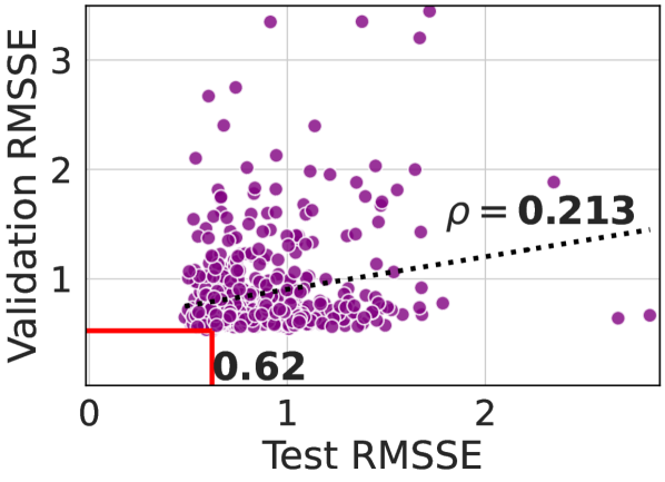
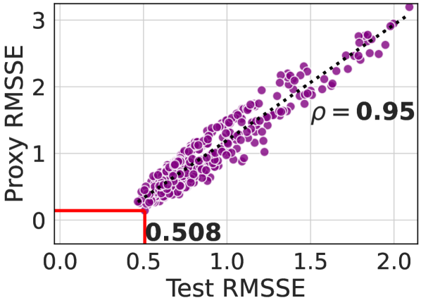
(a) Tourism  data

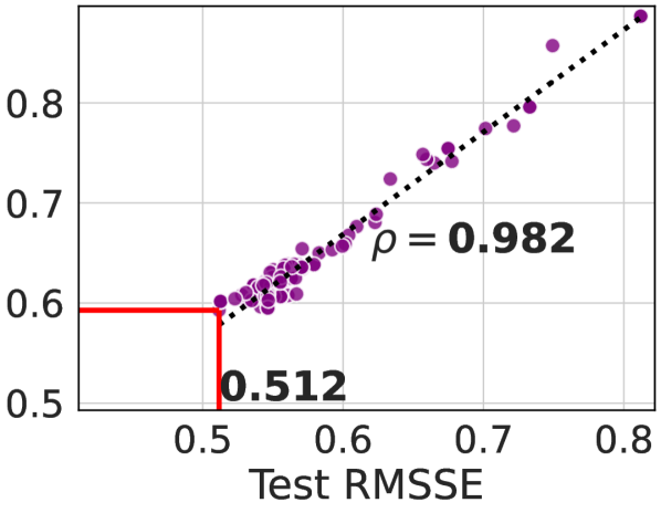
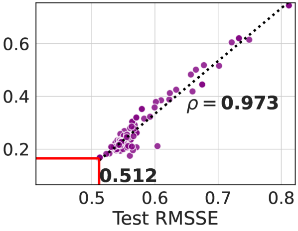
(b) Tourism-L  data

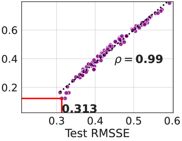
(c) Wiki  data

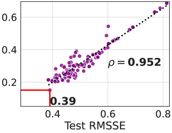
(d) Traffic  data

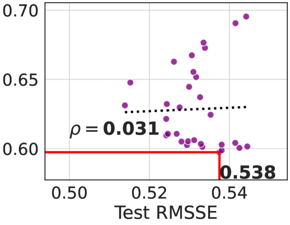
(e) M5-Dept. data

Figure 3. Test errors vs. validation errors (upper figure for each subplot). Test errors vs. proxy errors (lower figure for each subplot). The solid purple circles denote the HPO trials. Linear trend is shown with the dotted black line, along with Pearson correlation value ($\rho$). The red horizontal line denotes the minimum validation (or, proxy) error, and the corresponding test error is annotated beside the red vertical line. The plots are shown for one random seed. For M5-Store, refer to Figure 1. Best viewed in color.

5.5.2. Teacher selection and ensemble modeling

As shown in Theorem 4.4, an accurate teacher helps the student to produce accurate higher-level forecasts. However, in Section 5.3 and 5.4, we saw that the two variants of H-Pro (H-Pro-Avg and H-Pro-Top) built with two configurations of the teacher can achieve the best results interchangeably across datasets. For example, in M5, teacher’s test accuracy in L1 is good but poor in other levels. Hence, we observe H-Pro-Top outperforms SOTA while H-Pro-Avg fails, as shown in Table 4. In practice, since the teacher’s test accuracy is not known, we would need a mechanism to achieve stable performance of H-Pro Top and H-Pro-Avg across datasets. To address this, we build ensemble models between different variants of H-Pro. We use the mean of the forecasts from multiple models for ensembles. As an ablation study, we also build ensemble models between H-Pro and TCV baselines. We denote these ensembles with the following numbers for concise representation in Table 6. (1) H-Pro-Avg and H-Pro-Top, (2) H-Pro-Avg-PO and H-Pro-Top-PO, (3) 1 and 2, (4) 3 and the best TCV baseline as obtained in Table 2. In all datasets, the ensembles perform better than the baselines. We can see that the ensemble among all H-Pro variants (id=3) outperforms the best SOTAs and baselines across all five datasets, and hence, can be considered a more stable version of H-Pro, which is more robust to possible sub-optimal teacher performance. Moreover, ensembles of H-Pro variants and TCV improve the performance of the latter, which is beneficial as it shows complementary information was integrated by our approach.

5.5.3. Correlation study

Figure 3 plots the test errors in different HPO trials with respect to validation (or, proxy) errors in those trials for all five datasets used in our experiment. We present the plots for TCV-Hier  and H-Pro-Top  variants. The linear trend lines are also shown along with Pearson correlation values. It is evident that H-Pro  obtains much better correlation than TCV  for Tourism, Wiki, M5-Department, and M5-Store data (for the last one, refer to Figure 1). Hence, HPO trial chosen with the best proxy error often corresponds to better (sometimes the best) test error. On the other hand, HPO trial selected with the best validation error often results in worse test errors in those scenarios. For Traffic  data, in the specific random experiment dictated by the seed, we see that TCV-Hier  obtains better test error than H-Pro-Top, but the correlation score is higher in the latter. For Tourism-L  data, the scatter plots look similar which is expected from their similar performance (refer to Table 2). Overall, in five out of six scenarios, we see H-Pro’s proxy error to have better correlation with the actual test error. This highlights the benefits of our approach in performing HPO with proxy errors, particularly when there is a potential mismatch between the validation and test periods (e.g., in M5).

5.5.4. Adaptation to new test window

Although, H-Pro is targeted to a particular test-window, we can easily tune it to new test windows by leveraging the saved models from the previous HPO run. H-Pro only requires recomputing the predictions and evaluating the HPO objective for every trial in the past HPO run to select the best model for the new test window. Thus, retraining for all the HPO trials is not mandatory for H-Pro, leading to faster adaptation to newer test windows. We should note that, often in forecasting, the immediate past is utilized in training. In that scenario, H-Pro and TCV both need to rerun full HPO.

6. Concluding remarks

We proposed a hierarchical proxy-guided HPO method for hierarchical time series forecasting to mitigate the perennial problem of data mismatch between validation and test periods in real-life time series. We provided theoretical justification of the approach along with extensive empirical evidence. The main benefit of the proposed approach is that it is essentially a model selection or HPO method that can be applied to any off-the-shelf machine/deep learning model for hierarchical time series forecasting. We validated H-Pro-based HPO with classical machine learning as well as deep learning models in our experiments. H-Pro  outperformed the conventional temporal cross-validation based HPO approaches in all datasets. It also achieves superior results than well-established state-of-the-art methods in four forecasting datasets, and competitive result in one dataset. The performance gain is observed in datasets from diverse domains without requiring any model-specific enhancements.

A future extension can be on formulating a fractional confidence score for the teacher at a certain higher-level node so that the suboptimal teacher forecasts can be given lower priority during the HPO of the student model. H-Pro  can also be extended to other domains (such as computer vision) when the dataset possesses an inherent hierarchical structure (e.g., in hierarchical image recognition).

Appendix

Appendix A Advantages of H-Pro over existing reconciliation methods

State-of-the-art reconciliation methods like MinT and ERM  try to factor in forecasts at all levels to derive the final adjusted forecasts, but these have several shortcomings.  First, they are generally not scalable to large number of time series, since they at least require fitting parameter matrices that have size on the order of $N\times N$ where $N$ is the number of base time series.  This fitting essentially requires multiple matrix inversions of matrices of this size (which has complexity more than $O(N^{4})$), or for the best performing ERM, solving an even bigger regression problem with $O(TN^{2})$ data points (where $T$ is the number of historical time points) and $O(N^{2})$ variables.  Additionally they add significant complexity to the forecast process (i.e., getting all hierarchy forecasts on historical data, fitting the reconciliation model, getting forecasts and applying reconciliation model at test time to adjust base forecasts, etc.), and can suffer from overfitting especially with modern ML and DL forecasting approaches that may have close to zero training error, since typically training data forecasts are used to fit the reconciliation model.

Furthermore, both these and the simpler top-down / middle-out reconciliation approaches use fixed linear combinations of different series’ forecasts (a single series in the case of top-down and middle-out) to get the adjusted base forecasts, which can be insufficient to accurately predict the base level when the relationship between the levels is more complex (e.g., nonlinear) or changes over time, which is a common case as different local effects can cause proportions relative to aggregates to shift (e.g., consider events like promotion, price change, or advertisement in a retail setting, causing demand and sales for one product to shift to another).

H-Pro on the other hand adjusts the selected base level forecasters directly by leveraging aggregate-level information, hence, can still have time-evolving changes in relative proportions for base level series that factor in all local information. Additionally it avoids having to fit a reconciliation model and apply a complex reconciliation process so it is much more scalable, simpler, and easier to use. While it does require some aggregate level forecasts, these are only needed for the test periods used for model selection.

Appendix B Proofs

B.1. Proof of Lemma 4.3

This can proved trivially, by employing Definition 4.1 in (4), and comparing with (4.2).

B.2. Proof of Theorem 4.4

Proof.

Following (4),

(7) $$\mathcal{O}=\frac{1}{L-1}\sum_{l=1}^{L-1}\frac{1}{N_{l}}\sum_{j=1}^{N_{l}}\frac{1}{H}\sum_{t=T+1}^{T+H}\left(\tilde{x}_{t}^{l,j}-\hat{x}_{t}^{l,j}\right)^{2},$$

where, we denote $\hat{x}_{t}^{l,j}=\mathcal{B}\left(f_{\lambda},\left\{x^{L,i}_{1:T}\right\}_{i=1}^{N_{L}},l,j\right)$ for compactness. Following (4.2),

(8) $$\mathcal{O}^{\ast}=\frac{1}{L-1}\sum_{l=1}^{L-1}\frac{1}{N_{l}}\sum_{j=1}^{N_{l}}\frac{1}{H}\sum_{t=T+1}^{T+H}\left(x_{t}^{l,j}-\hat{x}_{t}^{l,j}\right)^{2}.$$

To make the equations concise, let

(9) $$\mathcal{S}\left(\cdot\right)=\frac{1}{L-1}\sum_{l=1}^{L-1}\frac{1}{N_{l}}\sum_{j=1}^{N_{l}}\frac{1}{H}\sum_{t=T+1}^{T+H}(\cdot).$$

Hence,

(10) $$\mathcal{O}=\mathcal{S}\left(\tilde{x}_{t}^{l,j}-\hat{x}_{t}^{l,j}\right)^{2}$$

(11) $$\mathcal{O}^{\ast}=\mathcal{S}\left(x_{t}^{l,j}-\hat{x}_{t}^{l,j}\right)^{2}.$$

Hence,

$$\biggl{|}\mathcal{O}\biggl{.} -\mathcal{O}^{\ast}\biggr{|}\biggr{.}$$

$$=\left|\mathcal{S}\left(\left(\tilde{x}_{t}^{l,j}-\hat{x}_{t}^{l,j}\right)^{2}-\left(x_{t}^{l,j}-\hat{x}_{t}^{l,j}\right)^{2}\right)\right|$$

$$=\left|\mathcal{S}\left(\left(\tilde{x}_{t}^{l,j}-x_{t}^{l,j}\right)\left(\tilde{x}_{t}^{l,j}-2\hat{x}_{t}^{l,j}+x_{t}^{l,j}\right)\right)\right|$$

$$=\left|\mathcal{S}\left(\left(\tilde{x}_{t}^{l,j}-x_{t}^{l,j}\right)\left(2\left(x_{t}^{l,j}-\hat{x}_{t}^{l,j}\right)+\left(\tilde{x}_{t}^{l,j}-x_{t}^{l,j}\right)\right)\right)\right|.$$

Applying triangle inequality ($|a+b|\leq|a|+|b|$),

$$\biggl{|}\mathcal{O}\biggl{.} -\mathcal{O}^{\ast}\biggr{|}\biggr{.}$$

$$\leq\mathcal{S}\left(\left|\left(\tilde{x}_{t}^{l,j}-x_{t}^{l,j}\right)\left(2\left(x_{t}^{l,j}-\hat{x}_{t}^{l,j}\right)+\left(\tilde{x}_{t}^{l,j}-x_{t}^{l,j}\right)\right)\right|\right)$$

$$=\mathcal{S}\left(\left|\tilde{x}_{t}^{l,j}-x_{t}^{l,j}\right|\left|2\left(x_{t}^{l,j}-\hat{x}_{t}^{l,j}\right)+\left(\tilde{x}_{t}^{l,j}-x_{t}^{l,j}\right)\right|\right).$$

Applying triangle inequality again on the inner term,

$$\biggl{|}\mathcal{O}\biggl{.} -\mathcal{O}^{\ast}\biggr{|}\biggr{.}$$

$$\leq\mathcal{S}\left(\left|\tilde{x}_{t}^{l,j}-x_{t}^{l,j}\right|\left(\left|2\left(x_{t}^{l,j}-\hat{x}_{t}^{l,j}\right)\right|+\left|\tilde{x}_{t}^{l,j}-x_{t}^{l,j}\right|\right)\right)$$

$$=\mathcal{S}\left(\left|\tilde{x}_{t}^{l,j}-x_{t}^{l,j}\right|^{2}\right)+2\mathcal{S}\left(\left|\tilde{x}_{t}^{l,j}-x_{t}^{l,j}\right|\left|x_{t}^{l,j}-\hat{x}_{t}^{l,j}\right|\right)$$

Let $\mathcal{E}$ denote the aggregated mean squared error of teacher’s proxy forecasts in all higher levels. Formally,

(13) $$\mathcal{E} =\frac{1}{L-1}\sum_{l=1}^{L-1}\frac{1}{N_{l}}\sum_{j=1}^{N_{l}}\frac{1}{H}\sum_{t=T+1}^{T+H}\left(\tilde{x}_{t}^{l,j}-x_{t}^{l,j}\right)^{2}$$

(14) $$=\mathcal{S}\left(\left|\tilde{x}_{t}^{l,j}-x_{t}^{l,j}\right|^{2}\right).$$

Substituting (14) in (LABEL:app:eq:O-minus-O-star),

$$\biggl{|}\mathcal{O}\biggl{.} -\mathcal{O}^{\ast}\biggr{|}\biggr{.}$$

$$\leq\mathcal{E}+\frac{2}{L-1}\sum_{l=1}^{L-1}\frac{1}{N_{l}}\sum_{j=1}^{N_{l}}\frac{1}{H}\sum_{t=T+1}^{T+H}\epsilon_{t}^{l,j}\delta_{t}^{l,j}.$$

∎

B.3. Example of reduced variance at higher level

For the toy hierarchy shown in Figure 2, let $X_{1}$ and $X_{2}$ be the time series values at the the leaf nodes, and $Y$ the aggregated sum at the parent. Assume $X_{1}$, $X_{2}$ are jointly normal random variables with the following mean and covariance:

(15) $$\bm{\mu}=\begin{bmatrix}\mu_{1}\\ \mu_{2}\end{bmatrix},\\ \quad\bm{\Sigma}=\begin{bmatrix}\sigma_{1}^{2}&\rho\sigma_{1}\sigma_{2}\\ \rho\sigma_{1}\sigma_{2}&\sigma_{2}^{2}\end{bmatrix}.$$

Then $Y=X_{1}+X_{2}$ is also normally distributed:

(16) $$Y\sim\mathcal{N}\left(\mu_{1}+\mu_{2},\sigma_{1}^{2}+\sigma_{2}^{2}+2\rho\sigma_{1}\sigma_{2}\right)$$

If we assume $\sigma_{1}=\sigma_{2}=\sigma$, then for $\rho\leq-0.5$,

(17) $$\sigma_{Y}^{2}\leq\sigma^{2}\,.$$

References

- (1)
- Abdallah et al. (2022) Mustafa Abdallah, Ryan Rossi, Kanak Mahadik, Sungchul Kim, Handong Zhao, and Saurabh Bagchi. 2022. AutoForecast: Automatic Time-Series Forecasting Model Selection. In Proceedings of the 31st ACM International Conference on Information & Knowledge Management. 5–14.
- Akgiray (1989) Vedat Akgiray. 1989. Conditional heteroscedasticity in time series of stock returns: Evidence and forecasts. Journal of business 62, 1 (1989), 55–80.
- Anderer and Li (2021) Matthias Anderer and Feng Li. 2021. Forecasting reconciliation with a top-down alignment of independent level forecasts. arXiv preprint arXiv:2103.08250 (2021).
- Assimakopoulos and Nikolopoulos (2000) Vassilis Assimakopoulos and Konstantinos Nikolopoulos. 2000. The theta model: a decomposition approach to forecasting. International journal of forecasting 16, 4 (2000), 521–530.
- Ben Taieb and Koo (2019) Souhaib Ben Taieb and Bonsoo Koo. 2019. Regularized regression for hierarchical forecasting without unbiasedness conditions. In Proceedings of the 25th ACM SIGKDD International Conference on Knowledge Discovery & Data Mining. 1337–1347.
- Bergstra and Bengio (2012) James Bergstra and Yoshua Bengio. 2012. Random search for hyper-parameter optimization. Journal of machine learning research 13, 2 (2012), 281–305.
- Bergstra et al. (2013) James Bergstra, Daniel Yamins, and David Cox. 2013. Making a science of model search: Hyperparameter optimization in hundreds of dimensions for vision architectures. In Proceedings of the 30th International Conference on Machine Learning, Vol. 28. PMLR, 115–123.
- Das et al. (2022) Abhimanyu Das, Weihao Kong, Biswajit Paria, and Rajat Sen. 2022. A Top-Down Approach to Hierarchically Coherent Probabilistic Forecasting. arXiv preprint arXiv:2204.10414 (2022).
- Deng et al. (2023) Difan Deng, Florian Karl, Frank Hutter, Bernd Bischl, and Marius Lindauer. 2023. Efficient automated deep learning for time series forecasting. In Machine Learning and Knowledge Discovery in Databases: European Conference, ECML PKDD 2022, Grenoble, France, September 19–23, 2022, Proceedings, Part III. Springer, 664–680.
- Dua and Graff (2017) Dheeru Dua and Casey Graff. 2017. UCI Machine Learning Repository. http://archive.ics.uci.edu/ml. University of California, Irvine, School of Information and Computer Sciences”.
- Hinton et al. (2015) Geoffrey Hinton, Oriol Vinyals, Jeff Dean, et al. 2015. Distilling the knowledge in a neural network. arXiv preprint arXiv:1503.02531 2, 7 (2015).
- Hyndman and Athanasopoulos (2021) R.J. Hyndman and G. Athanasopoulos (Eds.). 2021. Forecasting: principles and practice. OTexts: Melbourne, Australia. OTexts.com/fpp3.
- Liaw et al. (2018) Richard Liaw, Eric Liang, Robert Nishihara, Philipp Moritz, Joseph E Gonzalez, and Ion Stoica. 2018. Tune: A Research Platform for Distributed Model Selection and Training. arXiv preprint arXiv:1807.05118 (2018).
- Makridakis et al. (2022) Spyros Makridakis, Evangelos Spiliotis, and Vassilios Assimakopoulos. 2022. M5 accuracy competition: Results, findings, and conclusions. International Journal of Forecasting (2022). https://www.sciencedirect.com/science/article/pii/S0169207021001874 https://doi.org/10.1016/j.ijforecast.2021.11.013.
- Mancuso et al. (2021) Paolo Mancuso, Veronica Piccialli, and Antonio M Sudoso. 2021. A machine learning approach for forecasting hierarchical time series. Expert Systems with Applications 182 (2021), 115102. https://doi.org/10.1016/j.eswa.2021.115102.
- Oreshkin et al. (2020) Boris N Oreshkin, Dmitri Carpov, Nicolas Chapados, and Yoshua Bengio. 2020. N-BEATS: Neural basis expansion analysis for interpretable time series forecasting. In International Conference on Learning Representations. https://openreview.net/forum?id=r1ecqn4YwB.
- Paria et al. (2021) Biswajit Paria, Rajat Sen, Amr Ahmed, and Abhimanyu Das. 2021. Hierarchically regularized deep forecasting. arXiv preprint arXiv:2106.07630 (2021).
- Rangapuram et al. (2021) Syama Sundar Rangapuram, Lucien D Werner, Konstantinos Benidis, Pedro Mercado, Jan Gasthaus, and Tim Januschowski. 2021. End-to-end learning of coherent probabilistic forecasts for hierarchical time series. In International Conference on Machine Learning. PMLR, 8832–8843.
- Salinas et al. (2020) David Salinas, Valentin Flunkert, Jan Gasthaus, and Tim Januschowski. 2020. DeepAR: Probabilistic forecasting with autoregressive recurrent networks. International Journal of Forecasting 36, 3 (2020), 1181–1191.
- Taieb et al. (2017) Souhaib Ben Taieb, James W Taylor, and Rob J Hyndman. 2017. Coherent probabilistic forecasts for hierarchical time series. In International conference on machine learning. PMLR, 3348–3357.
- Tourism Australia, Canberra (2005) Tourism Australia, Canberra. 2005. Tourism Research Australia (2005), Travel by Australians. Accessed at https://robjhyndman.com/publications/hierarchical-tourism/.
- Wickramasuriya et al. (2019) Shanika L Wickramasuriya, George Athanasopoulos, and Rob J Hyndman. 2019. Optimal forecast reconciliation for hierarchical and grouped time series through trace minimization. J. Amer. Statist. Assoc. 114, 526 (2019), 804–819.
- Wikistats (2016) Wikistats. 2016. Wikistats: Pageview complete dumps, Wikimedia Analytics team. Accessed at https://dumps.wikimedia.org/other/pageview _complete/readme.html.
- Zhou et al. (2021) Haoyi Zhou, Shanghang Zhang, Jieqi Peng, Shuai Zhang, Jianxin Li, Hui Xiong, and Wancai Zhang. 2021. Informer: Beyond efficient transformer for long sequence time-series forecasting. In Proceedings of the AAAI Conference on Artificial Intelligence, Vol. 35. 11106–11115.