Helical topological superconductivity in intrinsic quantum Hall superconductors

Abstract

One of the approaches to engineering topological superconductivity in a two dimensional electron gas with spin-orbit coupling is to proximity-couple it to an s-wave type-II superconductor with a non-standard Abrikosov flux lattice that is neither triangular or square but has an even number of superconducting flux quanta per unit cell. Here we ask whether exposing an intrinsic two-dimensional superconductor with spin orbit coupling to a perpendicular magnetic field – an intrinsic quantum Hall superconductor – can give rise to topological superconductivity. We investigate this question in a mean-field theory and obtain, in a self-consistent fashion, the real space configuration of the superconducting order parameter, which encodes information about the topology of the superconductivity as well as the nature of the Abrikosov lattice. We find small regions of topological superconductivity in the parameter space, which can be greatly enlarged by the addition of a superlattice potential. Topological superconductivity is seen to be correlated with the presence of either a distorted Abrikosov lattice or an Abrikosov lattice of giant vortices which carry two superconducting flux quanta. To identify the lowest energy solution, it is essential to employ helical order parameters. Finally, we discuss the experimental feasibility of this proposal.

I Introduction

Majorana modes, which are quasiparticles which may be considered as their own anti-particles, are perhaps the most readily realizable non-Abelian anyons. In topological superconductors, they appear as zero-energy quasiparticles which reside in the cores of Abrikosov vortices, or appear as chiral boundary modes. Their non-Abelian braid statistics, although not yielding all unitary gates, are a major step towards topological quantum computation with anyons Stone and Chung (2006); Oshikawa et al. (2007); Nayak et al. (2008); Sau et al. (2010a); Stanescu et al. (2010); Alicea (2012); Hung et al. (2013); Beenakker (2013); Zhou et al. (2013); Biswas (2013); Sarma et al. (2015); Liu and Franz (2015); Murray and Vafek (2015); Smith et al. (2016). Besides their potential application for quantum computation and being of fundamental scientific interest, achieving Majorana modes in the lab could lead to the physical realization of interesting theoretical models, such as the Sachdev-Ye-Kitaev model Chowdhury et al. (2022). There are several candidate condensed matter systems which are thought to host Majorana modes, including the $\nu=5/2$ fractional quantum Hall effect Ma et al. (2022), two dimensional p-wave superconductors, and two dimensional films of ³He-A superfluid Bernevig (2013). In addition, there have been proposals to engineer topologically interesting structures which host Majorana modes. In particular, topological p-wave superconductivity (SC) is thought to arise when a spin-orbit coupled electron gas is proximity coupled to an s-wave superconductor, owing to the appearance of a single Fermi surface in certain parameter regimes Sarma et al. (2006); Fu and Kane (2008); Lutchyn et al. (2010); Qi et al. (2010); Sau et al. (2010b, c); Alicea (2010); Qi and Zhang (2011); Black-Schaffer (2011); Mourik et al. (2012); Nakosai et al. (2012); Stanescu and Tewari (2013); Goertzen et al. (2017); Lutchyn et al. (2018). Particularly notable are proposals for quasi-one dimensional systems, e.g. semiconductor wires Lutchyn et al. (2010); Sau et al. (2010c); Oreg et al. (2010); Mourik et al. (2012); Nadj-Perge et al. (2014); Liu et al. (2017); Frolov et al. (2020), magnetic atom chains Klinovaja et al. (2013); Li et al. (2014), and planar Josephson junctions Fornieri et al. (2019); Pientka et al. (2017), for realizing topological superconductivity (TSC). Some exciting progress has been made on that front Aghaee and et al. (2022).

In earlier work, Sau et al. proposed a heterostructure consisting of a spin-orbit coupled two-dimensional electron gas (2DEG) coupled to a ferromagnetic insulator and an s-wave superconductor Sau et al. (2010b, c). The ferromagnetic insulator causes a gap in the single-particle spectrum of the 2DEG at zero momentum. This gap, along with spin-orbit coupling (SOC), leads to the appearance of a single Fermi surface for certain values of the chemical potential. When the system is coupled to an s-wave superconductor, effective chiral p-wave TSC is realized in a single band. They studied the properties of the BdG spectrum in the regime where vortices are well-separated. Crucially for these works, it is the SOC, together with the Zeeman-like effect from the magnetic insulator, which gives rise to the topological phase.

A related idea is to apply a magnetic field to a two-dimensional system, utilizing the orbital effect to realize TSC. Indeed the topological nature of the underlying Landau levels (LLs) sets the stage nicely for TSC when a pairing gap is opened Qi et al. (2010); Qi and Zhang (2011). The combination of SC and quantum Hall (QH) systems, both integer (IQHE) and fractional (FQHE), has been thought to be fertile ground for the realization not only of TSC with the concomitant Majorana particles, but also more exotic topological phases that harbor parafermions and Fibonacci anyons Lu et al. (2010); Clarke et al. (2013); Mong et al. (2014); Alicea and Stern (2015); Alicea and Fendley (2016); Amet et al. (2016); Liang et al. (2019); Gül et al. (2022); Shaffer et al. (2021). In order to integrate the orbital effect of the magnetic field and SC, there are, broadly speaking, two approaches. The first, like the above proposal, involves proximity coupling a QH system to a superconductor. It is necessary to take into account the vortices in superconductors exposed to a magnetic field Zocher and Rosenow (2016); Mishmash et al. (2019); Jeon et al. (2019); Chaudhary and MacDonald (2020); Pathak et al. (2021); Tang et al. (2022); Schiller et al. (2022). Zocher and Rosenow Zocher and Rosenow (2016), Mishmash et al. Mishmash et al. (2019) and Chaudhary and MacDonald Chaudhary and MacDonald (2020) showed that there is no TSC for particles in the lowest LL (or lowest few LLs) if the unit cell of the Abrikosov lattice has only one (or in general an odd number of) superconducting flux quanta (that is, the unit cell violates magnetic translation symmetry), as is the case for the usual triangular Abrikosov lattice or even a square Abrikosov lattice. It was shown that the spectrum of the Bogoliubov-de Gennes (BdG) equations, which is com­pletely determined by the s-wave pairing potential when the normal state bands are flat, has an even degeneracy in the case of a square or triangular Abrikosov vortex lattice, and therefore any quasiparticle spectral gap clos­ing across a topological phase transition must lead to a Chern number change by an even integer, thereby precluding the appearance of TSC. All of these works considered LLs with spin-orbit coupling. Also, because they considered proximity-induced SC, they did not need to find a self-consistent mean-field state within the 2DEG, since the pairing, and consequently the Abrikosov lattice, are inherited from a nearby bulk superconductor, and hence are a part of the Hamiltonian defining the problem, not of its solution.

The second approach is to apply a strong magnetic field to an intrinsic two-dimensional superconductor, driving it into the Landau level limit. It has been known for some time that BCS mean field theory predicts that superconductivity can be enhanced due to the Landau level structure of systems in a strong magnetic field Rajagopal and Vasudevan (1991); Tesanovic et al. (1989, 1991); Norman (1991); Akera et al. (1991); Rajagopal and Vasudevan (1991); Rajagopal and Ryan (1991); Norman et al. (1991); Rasolt and Tesanovic (1992); MacDonald et al. (1992); Norman et al. (1992); Rajagopal (1992); MacDonald et al. (1993); Ryan and Rajagopal (1993a, b); Norman et al. (1995); Maśka (2002); Scherpelz et al. (2013); Ran et al. (2019); Kim et al. (2019); Chaudhary et al. (2021). Because of the enlargement of the density of states in Landau levels, it has been predicted that the critical temperature in this limit approaches that of the zero-field value Tesanovic et al. (1989, 1991). This has been referred to as quantum Hall superconductivity Chaudhary et al. (2021). In contrast to the case of proximity coupled SC to LLs, the vortex lattice structure is determined by electrons pairing in LLs within the same sample, and consequently a vortex lattice structure cannot be assumed but must be solved for self-consistently Akera et al. (1991); Norman et al. (1992); Ryan and Rajagopal (1993b). In spite of extensive theoretical work, convincing experimental demonstrations of these remarkable predictions have been lacking. In addition, to our knowledge, there has not been any study of the possibility of topological superconductivity in such systems. That is the focus of the present study.

In this work, we explore if TSC can arise from pairing between electrons occupying LLs, which may be referred to as “quantum Hall topological superconductivity.” For this purpose, we consider a fully self-consistent mean-field theory of a lattice model under a magnetic field with a phenomenological attractive on-site Hubbard interaction. We also consider Rashba SOC and a periodic superlattice potential. We numerically determine phase diagrams without SOC or superlattice potential, with SOC and without superlattice potential, without SOC and with superlattice potential, and with SOC and superlattice potential. We find that while SOC is necessary for TSC, the application of a superlattice potential markedly enlarges the regions hosting TSC in the phase diagram. In order to properly treat systems with a superlattice potential, we find it necessary to consider helical pairing functions, which describe Cooper pairs with non-zero center-of-mass momentum. We also describe vortex lattice structures arising in our model, some of which are quite unexpected. We finally discuss some prospective experimental realizations of this model.

II Model

II.1 Hamiltonian

We consider spin-$\frac{1}{2}$ fermions on a square lattice in a magnetic field with Rashba spin-orbit coupling (SOC), a single-particle potential, and onsite attractive interaction. The interacting Hamiltonian is

$$\mathcal{H}=\mathcal{H}_{0}+\mathcal{H}_{\rm SO}+\mathcal{H}_{\rm I},$$ (1)

where

$$\begin{split}\mathcal{H}_{0}=&-\sum_{j,\delta,\sigma}\Big{(}e^{iA_{\delta}(\bm{r}_{j})}c^{\dagger}_{j+\delta,\sigma}c_{j,\sigma}+e^{-iA_{\delta}(\bm{r}_{j})}c^{\dagger}_{j,\sigma}c_{j+\delta,\sigma}\Big{)}\\ &-\sum_{j,\sigma}\big{(}\mu-V(\bm{r}_{j})\big{)}c^{\dagger}_{j,\sigma}c_{j,\sigma}\\ \mathcal{H}_{\rm SO}=&V_{\rm SO}\sum_{j}\bigg{(}e^{iA_{\bm{\hat{x}}}(\bm{r}_{j})}\Big{(}c^{\dagger}_{j+\bm{\hat{x}},\downarrow}c_{j,\uparrow}-c^{\dagger}_{j+\bm{\hat{x}},\uparrow}c_{j,\downarrow}\Big{)}\\ &+ie^{iA_{\bm{\hat{y}}}(\bm{r}_{j})}\Big{(}c^{\dagger}_{j+\bm{\hat{y}},\downarrow}c_{j,\uparrow}+c^{\dagger}_{j+\bm{\hat{y}},\uparrow}c_{j,\downarrow}\Big{)}\bigg{)}+{\rm h.c.}\\ \mathcal{H}_{\rm I}=&-U\sum_{j}c^{\dagger}_{j,\uparrow}c^{\dagger}_{j,\downarrow}c_{j,\downarrow}c_{j,\uparrow},\end{split}$$ (2)

where $\bm{r}_{j}$ is the location of site $j$, $V_{\rm SO}$ is the SOC strength, $\mu$ is the chemical potential, $U$ is the interaction strength, $A_{\delta}(\bm{r}_{j})$ are the hopping (Peierls) phases, $\delta=\bm{\hat{x}},\bm{\hat{y}}$, $\sigma=\uparrow$, $\downarrow$. The annihilation (creation) operators for fermions of spin $\sigma$ at site $j$ are $c_{j,\sigma}$ ($c^{\dagger}_{j,\sigma}$). We have set the hopping amplitude to unity. Note that $A_{\delta}(\bm{r}_{j})$ appears both in the hopping term and the SOC term, which is necessary for gauge invariance. The Rashba SOC takes the form of the lattice-discretized version of $H_{R}=\alpha\hat{z}\cdot(\bm{\sigma\times\bm{\pi}})$ where $\bm{\pi}$ is the kinematic momentum (further discussion of this term can be found in the Supplementary Materials Schirmer et al. (2022)). Finally, we include a periodic single-particle potential of the form

$$V(\bm{r})=-\frac{V_{\rm sp}}{2}\sum_{\delta=\bm{\hat{x}},\bm{\hat{y}}}\cos\big{(}\bm{\eta}_{\delta}\cdot\bm{r}\big{)}$$ (3)

where $V_{\rm sp}$ is the strength of the periodic superlattice potential and $\eta_{x}$ and $\eta_{y}$ are the wavevectors of the periodic superlattice potential in the x and y directions, respectively.

II.2 Magnetic unit cell

A discussion of the translation symmetries of the non-interacting part of the Hamiltonian, i.e. $\mathcal{H}_{0}+\mathcal{H}_{\rm SO}$, is in order – we will discuss the interacting part $\mathcal{H}_{\rm I}$ below. The magnetic field in our model is chosen so that the magnetic flux through each square plaquette of the lattice is the same rational fraction $\alpha=1/q$ of the flux quantum $\Phi_{0}=h/e$. This rational fraction, and in particular the denominator $q$, determines the translation properties of the non-interacting Hamiltonian by constraining the unit cell of the system – called the magnetic unit cell (MUC) – to have a multiple of $q$ sites Harper (1955); Azbel (1964); Zak (1964a); Brown (1964); Zak (1964b); Hofstadter (1976). For our calculation, we choose $q=64$ and take the MUC to be a square consisting of either $8\times 8$ or $16\times 16$ sites. The total flux through the magnetic unit cell is thus either one or four flux quanta. Later, when we consider superconductivity arising from $\mathcal{H}_{\rm I}$, we will take the pairing potential to have the same periodicity as the MUC and thus choosing more flux quanta per MUC will restrict to a lesser degree the structure of the Abrikosov vortices, whose number per MUC is twice the number of flux quanta per MUC. (For example, a triangular lattice of Abrikosov vortices would not be allowed if only one flux quantum per MUC unit cell were used, but it would be allowed if 4 flux quanta per MUC were used.) The single-particle potential $V(\bm{r})$ is chosen to be commensurate with the magnetic unit cell, and in particular we take $(\eta_{x},\eta_{y})=(\frac{2\pi}{8},\frac{2\pi}{8})$. Previous authors Zocher and Rosenow (2016); Mishmash et al. (2019); Chaudhary and MacDonald (2020) have emphasized the need to break the translation symmetry of the vortex lattice in order to realize TSC in the presence of Abrikosov vortices. Our choice of single-particle potential accomplishes this, since the unit cell for the periodic potential contains one flux quantum $h/e$. In experiments, we expect that the magnetic length can be tuned to the wavelength of the periodic single-particle superlattice potential by tuning the magnetic field.

II.3 Mean-field theory

A mean-field factorization of the interacting part of the Hamiltonian $\mathcal{H}_{\rm I}$ is performed in the pairing channel

$$\begin{split}\mathcal{H}_{\rm I}=&-U\sum_{j}c^{\dagger}_{j,\uparrow}c^{\dagger}_{j,\downarrow}c_{j,\downarrow}c_{j,\uparrow}\\ \rightarrow&-U\sum_{j}\Big{(}\langle c_{j,\downarrow}c_{j,\uparrow}\rangle c^{\dagger}_{j,\uparrow}c^{\dagger}_{j,\downarrow}+\langle c^{\dagger}_{j,\uparrow}c^{\dagger}_{j,\downarrow}\rangle c_{j,\downarrow}c_{j,\uparrow}\\ &-\langle c^{\dagger}_{j,\uparrow}c^{\dagger}_{j,\downarrow}\rangle\langle c_{j,\downarrow}c_{j,\uparrow}\rangle\Big{)}\end{split}$$ (4)

In this work, we consider a mean-field ansatz of the form

$$\mathcal{H}_{\rm I}\rightarrow\mathcal{H}_{\Delta}=-\sum_{j}\Delta_{j}e^{i2\bm{Q}\cdot\bm{r}_{j}}c^{\dagger}_{j,\uparrow}c^{\dagger}_{j,\downarrow}+{\rm h.c.}+\sum_{j}\frac{|\Delta_{j}|^{2}}{U}$$ (5)

where the field $\Delta_{j}$ is assumed to be periodic with the same periodicity as the MUC. The vector $\bm{Q}$, which we will refer to as a boost vector, is treated as a variational parameter; the optimum $\bm{Q}$ is that which leads to a mean-field groundstate with the lowest energy. Note that, due to the phase factor $e^{i2\bm{Q}\cdot\bm{r}_{j}}$, the pairing potential in this model is not necessarily periodic. The addition of this phase factor gives the superconducting condensate a finite momentum $2\bm{Q}$ Yang and Agterberg (2000); Kaur et al. (2005); Agterberg and Kaur (2007); Agterberg (2012); Mironov and Buzdin (2017), although the groundstate with nonzero $\bm{Q}$ does not carry a finite net current .

The self-consistency equations are

$$\Delta_{j}e^{i2\bm{Q}\cdot\bm{r}_{j}}=U\langle\Gamma|c_{j,\downarrow}c_{j,\uparrow}|\Gamma\rangle$$ (6)

where $|\Gamma\rangle$ is the mean-field groundstate. In order to solve this equation, we first make a boost transformation on the mean-field Hamiltonian. A similar transformation has been employed in studies of helical phases in non-centrosymmetric superconductors Kaur et al. (2005); Agterberg and Kaur (2007); Agterberg (2012). We define boost operators $U_{B}(\bm{Q})$ which act on the creation operators in position space as

$$\bar{c}_{i,\sigma}\equiv U^{\dagger}_{B}(\bm{Q})c_{i,\sigma}U_{B}(\bm{Q})=c_{i,\sigma}e^{i\bm{Q}\cdot\bm{r}_{i}},$$ (7)

where the bar over the operators is meant to denote operators in a boosted ‘frame’. The mean-field Hamiltonian, defined as $\mathcal{H}_{\rm MF}=\mathcal{H}_{0}+\mathcal{H}_{\rm SO}+\mathcal{H}_{\Delta}$, is transformed using the boost operators. The action of the boosts on the terms $\mathcal{H}_{0}$ and $\mathcal{H}_{\rm SO}$ has the effect of shifting the hopping phases by $\bm{A}(\bm{r}_{j})\rightarrow\bm{A}(\bm{r}_{j})-\bm{Q}$. The boost has the effect on $\mathcal{H}_{\Delta}$ of cancelling the phase factor $e^{i2\bm{Q}\cdot\bm{r}_{j}}$. In other words,

$$\bar{\mathcal{H}}_{\Delta}=U^{\dagger}_{B}(\bm{Q})\mathcal{H}_{\Delta}U_{B}(\bm{Q})=-\sum_{j}\Delta_{j}c^{\dagger}_{j,\uparrow}c^{\dagger}_{j,\downarrow}+{\rm h.c.}+\sum_{j}\frac{|\Delta_{j}|^{2}}{U}$$ (8)

Thus the pairing Hamiltonian in the barred frame has the same periodicity as $\bar{\mathcal{H}}_{0}$ and $\bar{\mathcal{H}}_{\rm SO}$, and we can make use of the BdG formalism, using the magnetic Bloch basis, to solve the mean-field problem. The self-consistency equations in the barred frame are

$$\Delta_{j}=U\langle\bar{\Gamma}|c_{j,\downarrow}c_{j,\uparrow}|\bar{\Gamma}\rangle$$ (9)

where $|\bar{\Gamma}\rangle=U^{\dagger}_{B}(\bm{Q})|\Gamma\rangle$ is the mean-field groundstate in the barred frame.

II.4 Bogoliubov-de Gennes formalism

The mean-field Hamiltonian in the boosted frame can be expressed in terms of a BdG Hamiltonian by first transforming it into (magnetic) momentum space using the formula $c_{j,\sigma}=\frac{1}{L}\sum_{\bm{k}}e^{i\bm{k}\cdot\bm{R}_{j}}c_{\tilde{j},\sigma}(\bm{k})$, where $\bm{R}_{j}$ is the coordinate of the origin of the MUC in which site $j$ resides and $\tilde{j}$ denotes the site within the MUC of site $j$. In other words $\bm{r}_{j}=\bm{R}_{j}+\bm{\tilde{r}}_{j}$ where $\bm{\tilde{r}}_{j}$ is the coordinate of $\tilde{j}$ (relative to the origin of the MUC). $L$ is the number of MUCs in both the $x$ and $y$ directions; we consider $L$ large enough so that the results are converged to the thermodynamic limit, where we define convergence according to the following criterion: a solution $\Delta_{j}^{L}$ to Eq. (9) with system size $L$ is said to be converged to the thermodynamic limit if it is also a solution to Eq. (9) with system size $L+2$ to within the tolerance of the iterative algorithm used to solve Eq. (9) (see the Supplementary Materials for more details on the algorithm Schirmer et al. (2022)). Generally, we find that we need $L\geq 64$ for an $8\times 8$ MUC or $L\geq 32$ for a $16\times 16$ MUC for the pairing potential to be well converged. However we note that the Chern number (discussed below) is well-converged for much smaller system size – $L\approx 12$ for $8\times 8$ MUC or $L\approx 6$ for $16\times 16$ MUC.

The mean-field Hamiltonian may be written as

$$\begin{split}\bar{\mathcal{H}}_{\rm MF}=\frac{1}{2}\sum_{\bm{k}}\sum_{\alpha,\beta=1}^{4N_{\rm site}}\psi^{\dagger}_{\alpha}(\bm{k})\big{(}H_{\rm BdG}(\bm{k})\big{)}_{\alpha\beta}\psi_{\beta}(\bm{k})\\ +\frac{1}{2}\sum_{\bm{k}}\operatorname{Tr}\big{[}h(\bm{k})\big{]}+\sum_{j}\frac{|\Delta_{j}|^{2}}{U},\end{split}$$ (10)

where

$$\begin{pmatrix}\psi_{\tilde{j}}(\bm{k})\\ \psi_{\tilde{j}+N_{\rm site}}(\bm{k})\\ \psi_{\tilde{j}+2N_{\rm site}}(\bm{k})\\ \psi_{\tilde{j}+3N_{\rm site}}(\bm{k})\end{pmatrix}=\begin{pmatrix}c_{\tilde{j},\uparrow}(\bm{k})\\ c_{\tilde{j},\downarrow}(\bm{k})\\ c^{\dagger}_{\tilde{j},\uparrow}(-\bm{k})\\ c^{\dagger}_{\tilde{j},\downarrow}(-\bm{k})\end{pmatrix}$$ (11)

and

$$H_{\rm BdG}(\bm{k})=\\ =\begin{pmatrix}h(\bm{k})&\Sigma(\bm{k})&0&\Delta_{\uparrow\downarrow}(\bm{k})\\ \Sigma^{\dagger}(\bm{k})&h(\bm{k})&\Delta_{\downarrow\uparrow}(\bm{k})&0\\ 0&-\Delta_{\uparrow\downarrow}^{*}(-\bm{k})&-h^{*}(-\bm{k})&-\Sigma^{*}(\bm{-k})\\ -\Delta_{\downarrow\uparrow}^{*}(-\bm{k})&0&-\Sigma^{\rm T}(-\bm{k})&-h^{*}(-\bm{k})\end{pmatrix}$$ (12)

is the BdG Hamiltonian. $N_{\rm site}$ is the number of sites in the MUC. Each entry in Eq. (12) represents a matrix: $h(\bm{k})$ contains all the elements for hoppings (in the barred frame), the chemical potential, and the single-particle potential; $\Sigma(\bm{k})$ contains the SOC elements (in the barred frame), and $\Delta_{\uparrow\downarrow}(\bm{k})$ contains the pairing elements. Fermi statistics and Hermiticity imply $\Delta^{\rm T}_{\downarrow\uparrow}(\bm{k})=-\Delta_{\uparrow\downarrow}(-\bm{k})$. In our model, $\Delta_{\uparrow\uparrow}(\bm{k})=\Delta_{\downarrow\downarrow}(\bm{k})=0$ and $\Delta_{\downarrow\uparrow}(\bm{k})=-\Delta_{\uparrow\downarrow}(\bm{k})={\rm diag}(\Delta_{\tilde{j}})$. We define the BdG quasiparticle creation operators as

$$\gamma^{\dagger}_{\beta}(\bm{k})=\sum_{\alpha=1}^{4N_{\rm site}}\psi^{\dagger}_{\alpha}(\bm{k})\mathcal{U}_{\alpha\beta}(\bm{k})$$ (13)

By assumption, these are eigenoperators, so

$$\big{[}\mathcal{H}_{\rm MF},\gamma^{\dagger}_{\beta}(\bm{k})\big{]}=E_{\beta}(\bm{k})\gamma^{\dagger}_{\beta}(\bm{k}),$$ (14)

which implies that the columns of $\mathcal{U}_{\alpha\beta}$ must be eigenvectors of the BdG Hamiltonian

$$\sum_{\alpha=1}^{4N_{\rm site}}\big{(}H_{\rm BdG}(\bm{k})\big{)}_{\delta\alpha}\mathcal{U}_{\alpha\beta}(\bm{k})=E_{\beta}(\bm{k})\mathcal{U}_{\delta\beta}(\bm{k}).$$ (15)

We identify (15) as the BdG equations. The groundstate $|\bar{\Gamma}\rangle$ is obtained by filling the vacuum with the negative energy BdG quasiparticle states. The mean-field groundstate energy is given by

$$\mathcal{E}_{\rm MF}=\frac{1}{2}\sum_{E_{\beta}(\bm{k})<0}E_{\beta}(\bm{k})+\frac{1}{2}\sum_{\bm{k}}\operatorname{Tr}\big{[}h(\bm{k})\big{]}+\sum_{j}\frac{|\Delta_{j}|^{2}}{U}$$ (16)

II.5 Self-consistency equations

To solve the self-consistency equations, we define the Gor’kov Green’s function at momentum $\bm{k}$ as

$$\begin{split}\mathcal{G}_{\alpha\beta}(\bm{k})&=\langle\psi^{\dagger}_{\alpha}(\bm{k})\psi_{\beta}(\bm{k})\rangle\\ &=\sum_{m,n=1}^{4N_{\rm site}}\mathcal{U}^{\dagger}_{m\alpha}(\bm{k})\langle\gamma_{m}^{\dagger}(\bm{k})\gamma_{n}(\bm{k})\rangle\mathcal{U}_{\beta n}(\bm{k})\\ &=\sum_{m=1}^{4N_{\rm site}}\mathcal{U}^{\dagger}_{m\alpha}(\bm{k})\mathcal{U}_{\beta m}(\bm{k})f(E_{m}(\bm{k}))\end{split}$$ (17)

where $f(E)=\frac{1}{\exp(E/k_{B}T)+1}$ is the Fermi-Dirac distribution function. We consider only $T=0$ in this work. The self-consistency equations can be expressed in terms of $\mathcal{G}$ as

$$\begin{split}\Delta_{j}&=U\langle\bar{\Gamma}|c_{j,\downarrow}c_{j,\uparrow}|\bar{\Gamma}\rangle\\ &=\frac{U}{L^{2}}\sum_{\bm{k},\bm{k}^{\prime}}e^{i(\bm{k}+\bm{k}^{\prime})\cdot\bm{R}_{j}}\langle\bar{\Gamma}|c_{\tilde{j},\downarrow}(\bm{k}^{\prime})c_{\tilde{j},\uparrow}(\bm{k})|\bar{\Gamma}\rangle\\ &=\frac{U}{L^{2}}\sum_{\bm{k}}\mathcal{G}_{\tilde{j}+3N_{\rm site},\tilde{j}}(\bm{k})\end{split}$$ (18)

This equation is solved iteratively to achieve self-consistency.

II.6 Rationale for boosts

We consider superconductivity arising from Landau levels which are broadened by the presence of the single-particle potential in Eq. (3). A portion of the normal state spectrum (i.e. the energies of $\mathcal{H}_{0}+\mathcal{H}_{\rm SO}$) is shown in Fig. 1. Each band is spin-split due to the presence of SOC and, in contrast to a system without a single particle potential, the Landau levels are broadened and acquire a dispersion. The minima and maxima of the bands occur at non-zero momenta and consequently a pairing Hamiltonian describing pairs with finite momentum – that is, one that pairs particles at $\bm{Q}-\bm{k}$ and $\bm{Q}+\bm{k}$ – is required to open a superconducting gap at Fermi surfaces which appear when the chemical potential $\mu$ is tuned to within a band. Fig. 2 shows the condensation energy as a function of the boost momentum vector $\bm{Q}$. The stars indicate momenta corresponding to self-consistent mean-field states with the lowest energy, and it is at these momenta where a full pairing gap appears. An optimal boost moves the Fermi surface so that it becomes centered at $\bm{k}=\bm{G}/2$, where $\bm{G}$ is a reciprocal lattice vector (more information about the boost transformation can be found in the Supplemental Materials Schirmer et al. (2022)).

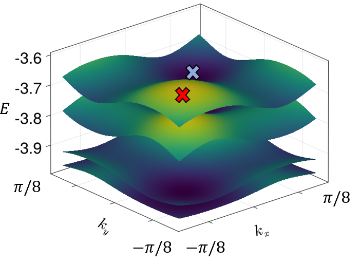
Figure 1: The energies of broadened Landau levels plotted in the magnetic Brillouin zone. The single particle potential strength is $V_{\rm sp}=0.2$ (in units where the hopping amplitude is set to unity). The flux per plaquette $\alpha=1/64$. The Rashba spin-orbit coupling strength is $V_{\rm SO}=0.1$. Because of the presence of the single-particle potential, the Landau levels become dispersive, and because of the spin-orbit coupling, the spin degeneracy is lifted. The maximum and minimum of the top band, which like the maxima and minima of other bands occur at finite momentum, are marked with a red and blue X, respectively

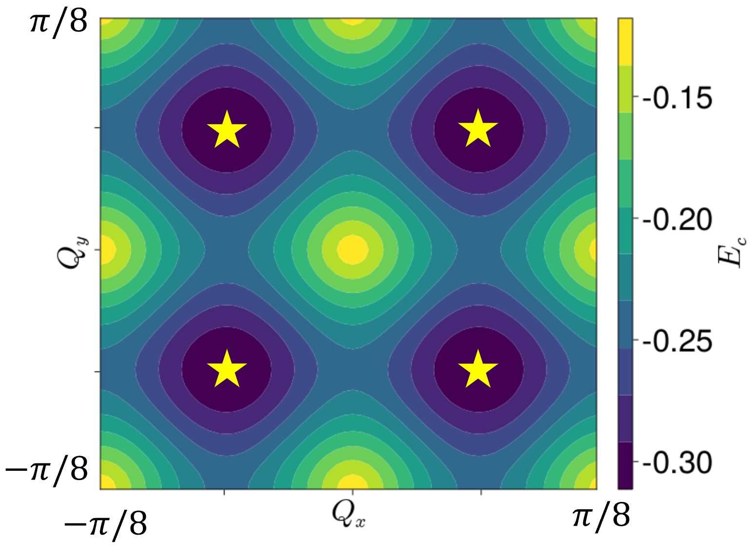
Figure 2: Condensation energy as a function of the boost vector $\bm{Q}$ for $V_{\rm sp}=0.1$, $V_{\rm SO}=0.1$, $U=3.2$, $\mu=-3.48$ in the magnetic Brillouin zone. The stars indicate the minimum energy states. Note that states differeing by a half reciprocal lattice vector have the same energy.

II.7 Chern number

We compute the Chern number, an integer-valued bulk topological invariant of the BdG Hamiltonian, to classify the system’s topology. The non-Abelian formalism is used to avoid having to keep track of topological transitions of bands far below the Fermi level. We define the Berry connection in terms of its eigenvectors $|u^{m}(\bm{k})\rangle$:

$$A^{mn}_{\mu}(\bm{k})=i\langle u^{m}(\bm{k})|\partial_{\mu}|u^{n}(\bm{k})\rangle,$$ (19)

where $\partial_{\mu}\equiv\partial/\partial{k_{\mu}}$, $\mu=x,y$ and $m,n$ are band indices. The Berry curvature is defined in terms of $A^{mn}_{\mu}(\bm{k})$

$$F^{mn}_{\mu\nu}(\bm{k})=\partial_{\mu}A^{mn}_{\nu}-\partial_{\nu}A^{mn}_{\mu}+i\left[{A}_{\mu},{A}_{\nu}\right]^{mn}$$ (20)

and the Chern number is given by the integral over states with negative energy of the BdG Hamiltonian

$$C=\frac{1}{2\pi}\int_{\rm MBZ}d^{2}k{\rm Tr}\left[{F}(\bm{k})\right]_{E(\bm{k})<0}$$ (21)

We numerically evaluate this integral using the method by Fukui, et. al Fukui et al. (2005) which is highly efficient for gapped systems. The Berry curvature is determined on a grid in a discretized MBZ by defining

$$M^{mn}_{\lambda}(\bm{k_{\alpha}})=\langle u^{m}(\bm{k_{\alpha}})|u^{n}(\bm{k_{\alpha}}+\bm{e}_{\lambda})\rangle.$$ (22)

The points on the grid are labeled by $\bm{k_{\alpha}}$ and the spacing vectors are $\bm{e}_{\lambda}$ where $\lambda=1,2$. In terms of the link variables defined as

$$U_{\lambda}(\bm{k_{\alpha}})=\frac{\det M_{\lambda}(\bm{k_{\alpha}})}{|\det M_{\lambda}(\bm{k_{\alpha}})|},$$ (23)

the discrete Berry curvature at each point on the grid is given by

$$\tilde{F}(\bm{k_{\alpha}})=\ln\Big{(}U_{1}(\bm{k_{\alpha}})U_{2}(\bm{k_{\alpha}}+\bm{e_{1}})\\ U_{1}^{-1}(\bm{k_{\alpha}}+\bm{e_{2}})U_{2}^{-1}(\bm{k_{\alpha}})\Big{)}$$ (24)

The Chern number is then given by

$$C=\frac{1}{2\pi i}\sum_{\bm{\alpha}}\tilde{F}(\bm{k_{\alpha}}).$$ (25)

When the Chern number is odd, the system is in the topological superconducting phase hosting non-Abelian Majorana quasiparticles. When the Chern number is even, the system does not host Majorana quasiparticles, and is in the same topological classification as a quantum Hall state. We find both possibilities in our results, but since both cases are, properly speaking, topological, we hereafter distinguish the former class of systems by referring to it as the non-Abelian topological phase.

III Results

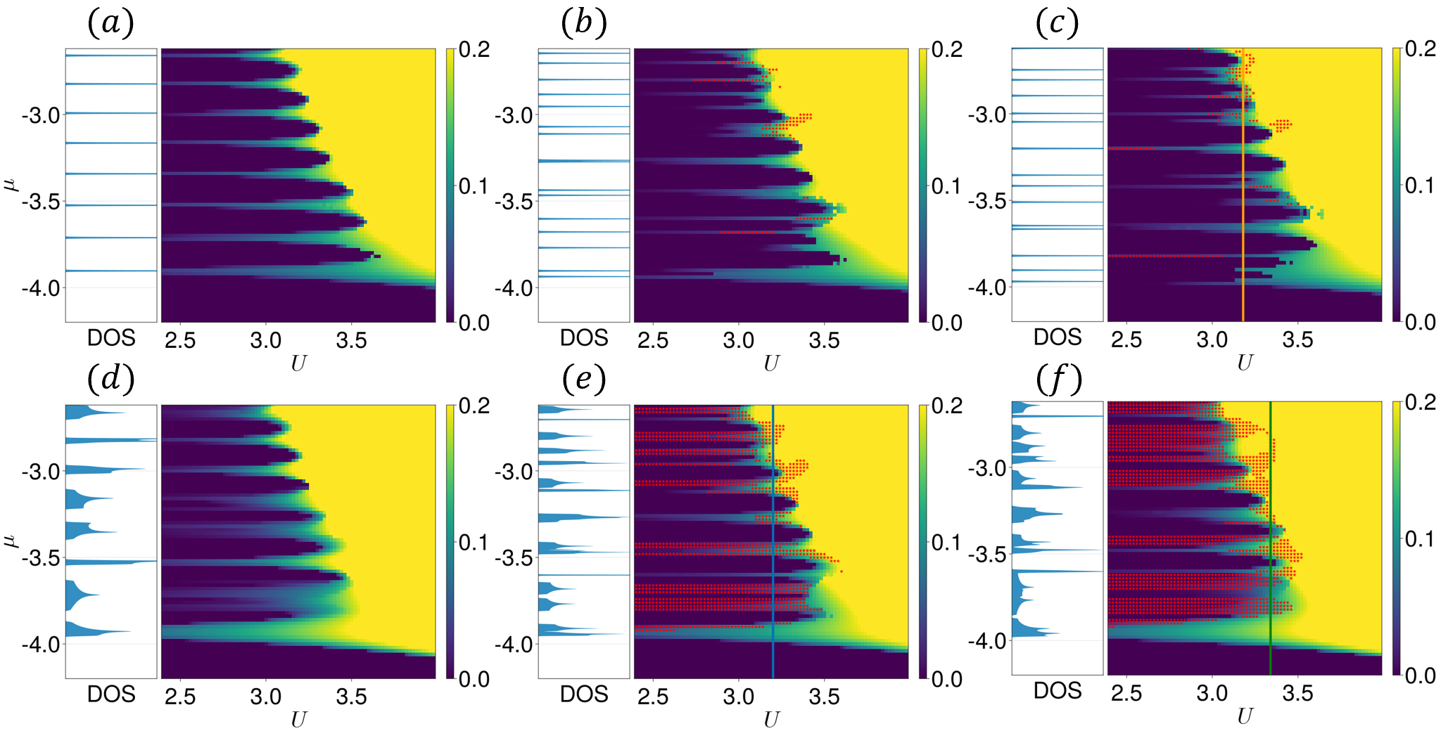
Figure 3: The density of states of the system in the normal state on the left and the phase diagram on the right showing $\Delta_{\rm max}$ (colorbar), the maximum value of the modulus of the self-consistent real space pairing potential $|\Delta_{j}|$ in the ground state. The points where non-Abelian topological superconductivity is realized are denoted with small red stars. The parameters for each phase diagram are (a) $V_{\rm SO}=0$ and $V_{\rm sp}=0$, (b) $V_{\rm SO}=0.1\approx\hbar\omega_{c}/2$ and $V_{\rm sp}=0$, (c) $V_{\rm SO}=0.15\approx 3/2\hbar\omega_{c}$ and $V_{\rm sp}=0$, (d) $V_{\rm SO}=0$ and $V_{\rm sp}=0.2\approx\hbar\omega_{c}$, (e) $V_{\rm SO}=0.1\approx\hbar\omega_{c}/2$ and $V_{\rm sp}=0.1\approx\hbar\omega_{c}/2$, (f) $V_{\rm SO}=0.1\approx\hbar\omega_{c}/2$ and $V_{\rm sp}=0.2\approx\hbar\omega_{c}$. The self consistency equations for all systems are solved, and the systems with a finite single-particle potential are boosted to an optimum value of $\bm{Q}$.

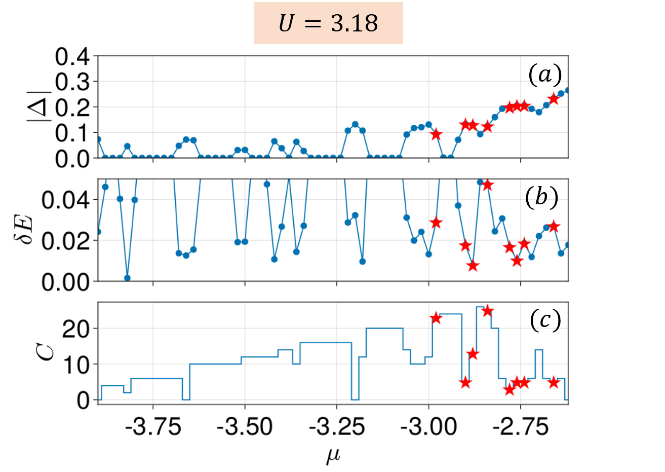
Figure 4: (a) The maximum absolute value of the pairing potential; (b) the BdG spectral gap ($\delta E$); and (c) the Chern number (C) for systems with chemical potentials along the orange line in Fig. 3 (c), at $U=3.18$. The blue dots and red stars indicate systems we have studied. Blue dots correspond to systems with even Chern number and red stars correspond to systems with odd Chern number.

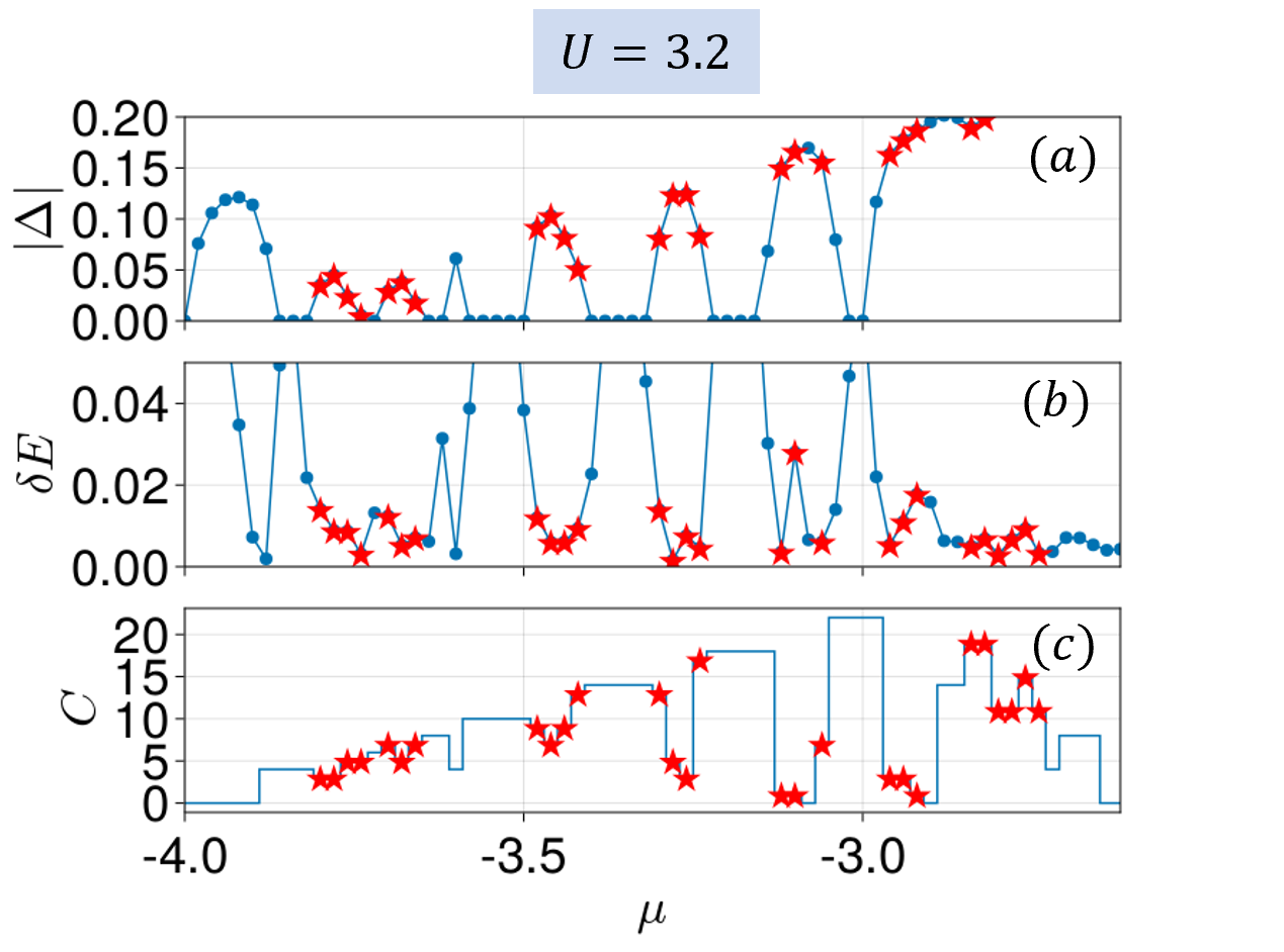
Figure 5: (a) The maximum absolute value of the pairing potential; (b) the BdG spectral gap ($\delta E$); and (c) the Chern number (C) for systems with chemical potentials along the blue line in Fig. 3 (c), at $U=3.2$. The blue dots and red stars indicate systems we have studied. Blue dots correspond to systems with even Chern number and red stars correspond to systems with odd Chern number.

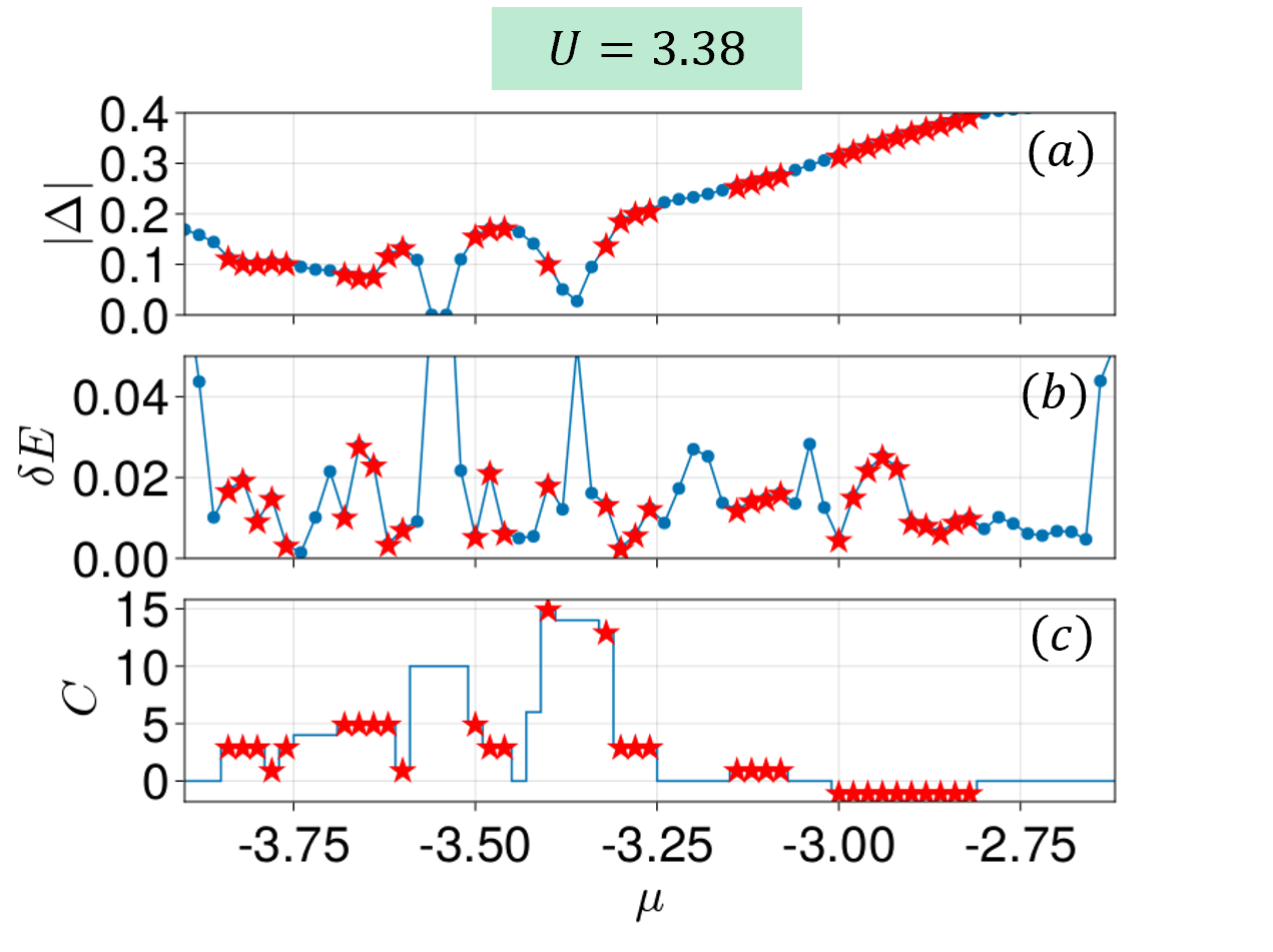
Figure 6: (a) The maximum absolute value of the pairing potential; (b) the BdG spectral gap ($\delta E$); and (c) the Chern number (C) for systems with chemical potentials along the blue line in Fig. 3 (c), at $U=3.38$. The blue dots and red stars indicate systems we have studied. Blue dots correspond to systems with even Chern number and red stars correspond to systems with odd Chern number.

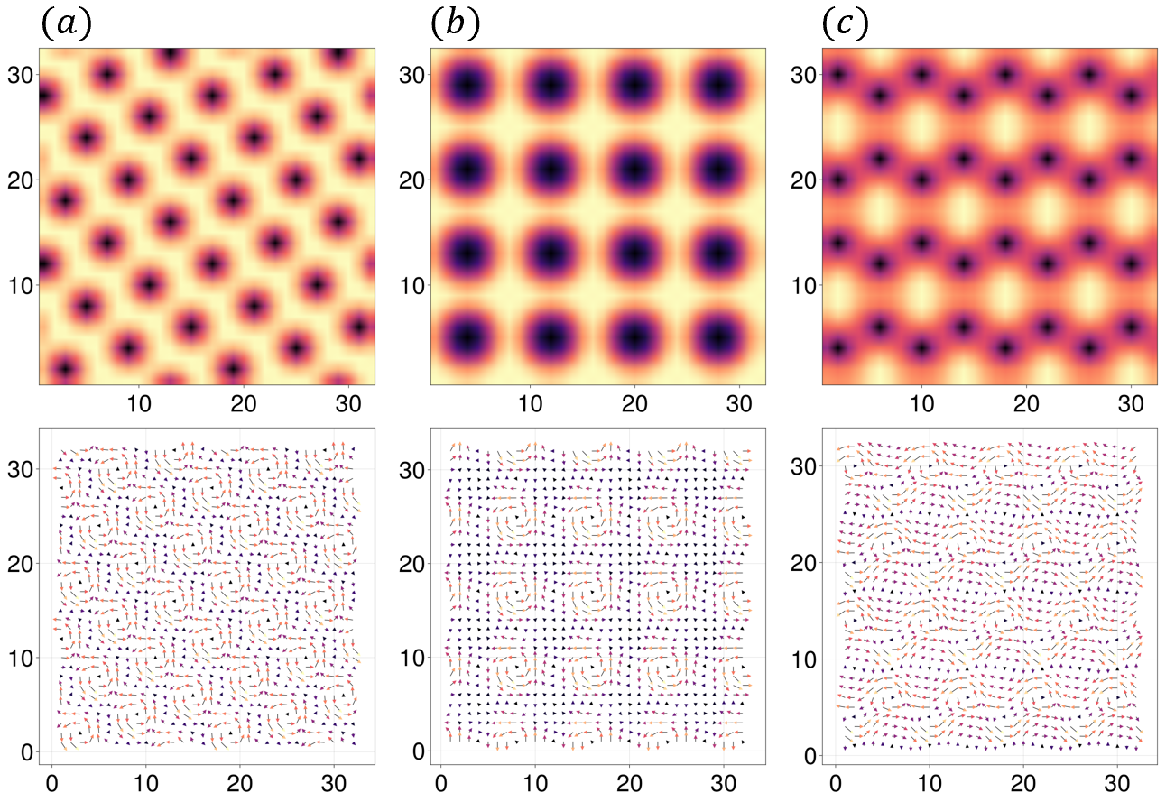
Figure 7: Typical vortex lattice structures from the solutions to the self-consistent mean field equations (upper panels) with their current textures (lower panels). (a) The vortex lattice at $V_{\rm sp}=0$, $V_{\rm SO}=0.1$, $U=3.52$, $\mu=-3.92$. In the lowest few Landau levels, the self-consistent solutions is a triangular lattice of Abrikosov vortices carrying flux $h/2e$. (b) The vortex lattice at $V_{\rm sp}=0.2$, $V_{\rm SO}=0.1$, $U=3.34$, $\mu=-3.66$. The single-particle potential distorts the vortex lattice, drawing the vortices to areas of high potential energy. Typically in the topological region, the system forms a lattice of giant vortices. (c) The vortex lattice at $V_{\rm sp}=0$, $V_{\rm SO}=0.1$, $U=3.24$, $\mu=-3.08$. Other kinds of vortex order form at higher chemical potential (Landau level filling factor $\nu\approx 10$). For example, the vortices may form a (distorted) honeycomb lattice.

We explored phase diagrams for a multitude of values of SOC and periodic potential strength for small Landau level filling factors (up to Landau level index $n=8$), as shown in Fig. 3. The self-consistent mean field equations were solved for each point on the phase diagrams, which each consist of 6400 ($80\times 80$) points. For each point, guesses consisting of random complex numbers at each site within the MUC, as well as uniform real numbers, were used to start the iterative algorithm, and $8\times 8$ (with flux $h/e$) or $16\times 16$ (with flux 4 $h/e$) MUCs were used. The total energy was calculated for each solution (Eq. 16) and the solution with the minimum energy was taken to be the groundstate solution. The color on the phase diagrams denotes $\Delta_{\rm max}$, the maximum value of the modulus of the self-consistent real space pairing potential $|\Delta_{j}|$ in the ground state. The points marked with red stars are points where the system is in the non-Abelian phase, i.e. the Chern number is an odd integer. The corresponding density of states (DOS) in the normal state is shown to the left of each phase diagram. Let us now consider four different cases:

No SOC or superlattice potential: Fig. 3(a) shows the phase diagram when both the SOC and single-particle potential are set to zero. The single particle spectrum consists of spin-degenerate Landau levels, which have a band width on the order of $10^{-14}$ and their spacing (the cyclotron energy $\hbar\omega_{c}$) is approximately 0.2. The phase boundary separating non-superconducting and superconducting regions of the phase diagram displays substantial oscillatory behavior due to the Landau level structure. At lower interaction strength, superconductivity is present when the chemical potential is tuned to precisely the energy of a Landau level, but disappears when it is tuned to the gaps between different Landau levels. We hereafter refer to regions of enhanced superconductivity at Landau level energies as Landau level spikes. At larger interaction strength ($U\geq 3.5$), superconductivity is strongly augmented, and oscillations due to the Landau level structure disappear. We will refer to this region as the strong pairing regime. The non-Abelian phase of topological superconductivity does not appear in the system without a periodic potential and SOC. Instead, the Chern numbers for all of the points shown are even integers. This follows from the spin degeneracy of the energy levels (see Supplementary Materials Schirmer et al. (2022)). In the weak interaction portion of the phase diagram, when the energies are between Landau level spikes, the Chern number is $2\nu$ where $\nu$ is the filling factor, consistent with the system being in a quantum Hall insulating phase. Within the Landau level spikes, the Chern number is an even integer, starting at $2\nu$ when the interaction is weak, and decreases in even increments as the interaction is increased, until the strong pairing regime where the Chern number is zero. It is interesting to note that superconductivity and nontrivial topology coincide on the Landau level spikes, although the topology is Abelian in nature.

SOC with no superlattice potential: Figs. 3 (b) and (c) show the phase diagrams of systems without the single particle potential but with SOC strength $V_{\rm SO}=0.1$ and $V_{\rm SO}=0.15$, respectively. Due to nonzero SOC, the spin degeneracy of the Landau levels is lifted, and the energies are given approximately by

$$\begin{split}\epsilon_{0}&=\frac{1}{2}\hbar\omega_{c}-4\\ \epsilon_{m,\pm}&=\hbar\omega_{c}\Bigg{(}m\pm\sqrt{\frac{\pi}{4}\frac{V_{\rm SO}^{2}}{\hbar^{2}\omega_{c}^{2}}m+\frac{1}{4}}\Bigg{)}-4~{}~{}~{}~{}(m>0)\end{split}$$ (26)

and accordingly there are Landau level spikes at these energies. Interestingly, we find small regions where the non-Abelian phase of topological superconductivity appears, most markedly at higher filling factors (at or around $\mu=-3$). For weaker interaction strength the Chern number at the non-Abelian points is an odd integer close to twice the filling factor, and decreases as the interaction strength is increased, until the Chern number becomes zero in the strong-pairing regime. The vortex structure at these points will be discussed below. We remark that we do not find non-Abelian TSC arising from superconductivity in the lowest Landau level, which has been the subject of recent studies Zocher and Rosenow (2016); Mishmash et al. (2019); Chaudhary and MacDonald (2020).

Plots of the maximum absolute value of the pairing potential, the BdG spectral gap ($\delta E$), and the Chern number (C), for chemical potentials along the orange line in Fig. 3 (c), at fixed $U=3.18$, are shown in Fig. 4. Points where the system is in the non-Abelian phase are denoted with red stars. Oscillations in Fig. 4 (a) which correspond to the Landau level spikes. The spectral gaps in Fig. 4 (b) come in two varieties: superconducting gaps and quantum Hall insulating gaps. The values of the quantum Hall insulating gaps, which occur when $\Delta=0$, are given by $2{\rm min}(|\mu-\epsilon_{m\pm}|)$, and are much larger than superconducting gaps. When $\Delta\neq 0$, the gaps are superconducting gaps. Generally, the superconducting gaps are small, about an order of magnitude less than the cyclotron energy, in the regime where non-Abelian TSC appears. Note that the Chern number may change without a closing of the spectral gap, see Fig. 4 (c) and cf. Fig. 4 (b), which suggest first-order transitions between states with different Chern numbers Ezawa et al. (2013).

Superlattice potential with no spin-orbit coupling: Fig. 3 (d) shows the phase diagram for the system with periodic potential strength $V_{\rm sp}=0.2$ but without spin-orbit coupling. The optimum boost vector is used for each point on the phase diagram. Despite the Landau levels becoming significantly broadened, as can be seen in the DOS and in the corresponding smearing of the Landau level spikes, the non-Abelian phase does not appear, and the system transitions from an Abelian TSC or quantum Hall insulating phase at weak interaction to trivial superconductivity at stronger interaction. It comes as no surprise that we do not find the non-Abelian phase when there is a spin degeneracy. This follows from Eqs. (19)-(21) and is established in detail in the Supplementary Materials (Schirmer et al. (2022)).

Both superlattice potential and SOC: Finally, including both a single-particle potential and SOC leads to a considerable enhancement of non-Abelian TSC in the phase diagram. Fig. 3 (e) shows the phase diagram for $V_{\rm sp}=0.1$ and $V_{\rm SO}=0.1$, and Fig. 3 (f) shows the phase diagram for $V_{\rm sp}=0.2$ and $V_{\rm SO}=0.1$. Non-Abelian TSC, which is marked using small red stars in the phase diagram, generally appears at the boundary between the quantum Hall insulator and superconducting phases, particularly along broadened Landau level spikes. Plots of the maximum absolute value of the pairing potential, the BdG spectral gap ($\delta E$), and the Chern number (C), for parameters along the blue line in Fig. 3 (e) and the green line in Fig. 3 (f), are shown in Fig. 5 and Fig. 6, respectively. Points where the system is in the non-Abelian phase are denoted with red stars. Oscillations can be seen in Fig. 5 (a), and to a lesser degree in Fig. 6 (a) (since the interaction strength is larger, the LL structure is more strongly altered by the pairing potential), which reflect the Landau level spikes. The spectral gaps are about an order of magnitude less than the cyclotron energy, at points where non-Abelian TSC appears. We again see that the Chern number may change despite the spectral gap not closing, indicating first-order transitions between states with different Chern numbers Ezawa et al. (2013).

III.1 Vortices and Majoranas

Due to the applied perpendicular magnetic field, the pairing potential experiences orbital frustration and Abrikosov vortices develop at the centers of which the pairing potential is zero. We find a plethora of configurations formed by the Abrikosov vortices, some of which are quite unexpected. As anticipated, Abrikosov vortices form a triangular lattice in the $n=0$ and $n=1$ Landau levels when the SOC and single-particle potential are absent. In addition we found square vortex lattice solutions with approximately $1-2\%$ higher energy than the triangular lattice solutions. With SOC, but without single-particle potential, a triangular lattice of vortices forms when the chemical potential is in the lowest 5 spin-split Landau levels – an example is shown in Fig. 7 (a). In both cases, at higher chemical potential, the vortex structure is far more diverse. Of particular note is the vortex structure at topological points in Figs. 3 (b) and (c), a typical example of which is shown in Fig. 7 (b). Here the vortices form a honeycomb lattice, although not all the bonds are identical. Other interesting structures appear in the non-topological regions in the strong pairing regime at chemical potential above the first few Landau levels. We show these in Fig. 4 of the Supplementary Materials Schirmer et al. (2022). Finally, when a single-particle potential is included, the vortices are distorted at all chemical potentials. In particular, vortices are drawn to locations where the single-particle potential is high. The vortices form dimer pairs (see Supplementary Materials Fig. 4 (a) Schirmer et al. (2022)), or combine to form giant vortices, consisting of two Abrikosov vortices. Topological points in Figs. 3 (e) and (f) typically host the latter configuration (Fig. 7 (b)).

As revealed by the finite gap when the system is in the non-Abelian topological phase, we do not find Majorana modes with zero energy in the bulk of the system. Instead the Majorana modes, which are thought to reside at vortex cores, hybridize with their neighbors and open a gap Grosfeld and Stern (2006); Cheng et al. (2009, 2010); Ludwig et al. (2011); Kraus and Stern (2011); Lahtinen et al. (2012); Laumann et al. (2012); Zhou et al. (2013); Biswas (2013); Silaev (2013); Murray and Vafek (2015); Liu and Franz (2015); Ariad et al. (2015); Li and Franz (2018); Mishmash et al. (2019). Nevertheless, because of the non-trivial Chern number and the bulk-boundary correspondence, we expect there to be chiral Majorana edge modes at the boundaries of samples in this phase.

IV Discussion

In this work, we investigated the emergence of TSC from topologically flat bands broadened by a superlattice potential. The robust SOC and the superlattice potential are essential components of our model. SOC has been experimentally demonstrated in a variety of superconducting compounds, including heavy fermion superconductor compound CePt₃Si Bauer et al. (2004); Frigeri et al. (2004), LaAlO₃/SrTiO₃ interface Caviglia et al. (2010); Reyren et al. (2007), transition metal dichalcogenides superconductors NbSe₂ ($T_{c}=$1-3 K, $H_{\rm c2}=1.4$ T, Ising SOC strength 49.8 meV) Xi et al. (2015, 2016); Ugeda et al. (2016); Wang et al. (2017); de la Barrera et al. (2018), WTe₂ and MoS₂ ($T_{c}=$9.4 K) Taniguchi et al. (2012), and iron-based superconductors Borisenko et al. (2016). Superlattice potentials can be realized by forming the moiré pattern of two-dimensional twisting materials with the well-known example of twisted bilayer graphene Andrei and MacDonald (2020). A superlattice potential has also been achieved by gating periodic patterned dielectric substrates Forsythe et al. (2018); Yankowitz et al. (2018); Shi et al. (2019); Xu et al. (2021); Li et al. (2021).

Previously, the helical phase of superconductors was discussed in the context of non-centrosymmetric superconductors using Ginzburg-Landau theory Agterberg (2003); Kaur et al. (2005); Agterberg and Kaur (2007); Agterberg (2012). Certain terms, known as Lifshitz invariants, can be eliminated from the free energy by performing a helical (or in our language, boost) transformation when inversion symmetry is broken. This is a similar procedure to the one we employ, albeit in a microscopic theory. However, even in the absence of Rashba spin-orbit coupling when inversion symmetry is preserved, helical transformations are necessary in our model because of the presence of a magnetic field and superlattice potential.

This work has demonstrated the dramatic influence on the vortex lattice structure by a superlattice potential, in the case of $\ell_{\rm B}/a_{\rm M}\approx 1$, where $\ell_{\rm B}$ is the magnetic length and $a_{\rm M}$ is the superlattice vector. Understanding the vortex lattice structure for other values of $\ell_{\rm B}/a_{\rm M}$, particularly irrational values, and the corresponding topological properties in this model, will be left for future work.

Finally, we would like to discuss some issues related to realizing intrinsic quantum Hall superconductivity. It has been over 50 years since quantum Hall superconductivity was first explored Rajagopal and Vasudevan (1966), however, due to the requirement of low densities or very high magnetic fields, it has not been achieved in experiments. In addition, theoretical studies on intrinsic quantum Hall superconductivity, including this one, have relied on mean-field theories which do not allow for all possible instabilities. In a real material, the interaction will be a mixture of attractive and repulsive, and this may lead to competition between other correlated phases including, but not limited to, FQHE, stripe phases, charge density waves, and spin density waves. The question of whether other strongly correlated phases may arise, particularly in the case of flat LLs, is an interesting question beyond mean-field theory, which we leave for the future.

References

- Stone and Chung (2006) M. Stone and S.-B. Chung, Physical Review B 73, 014505 (2006).
- Oshikawa et al. (2007) M. Oshikawa, Y. B. Kim, K. Shtengel, C. Nayak, and S. Tewari, Annals of Physics 322, 1477 (2007).
- Nayak et al. (2008) C. Nayak, S. H. Simon, A. Stern, M. Freedman, and S. Das Sarma, Reviews of Modern Physics 80, 1083 (2008).
- Sau et al. (2010a) J. D. Sau, R. M. Lutchyn, S. Tewari, and S. D. Sarma, Physical Review Letters 104, 040502 (2010a).
- Stanescu et al. (2010) T. D. Stanescu, J. D. Sau, R. M. Lutchyn, and S. D. Sarma, Physical Review B 81, 241310 (2010).
- Alicea (2012) J. Alicea, Reports on Progress in Physics 75, 076501 (2012).
- Hung et al. (2013) H.-H. Hung, P. Ghaemi, T. L. Hughes, and M. J. Gilbert, Physical Review B 87, 035401 (2013).
- Beenakker (2013) C. Beenakker, Annual Review of Condensed Matter Physics 4, 113 (2013).
- Zhou et al. (2013) J. Zhou, Y.-J. Wu, R.-W. Li, J. He, and S.-P. Kou, Europhysics Letters 102, 47005 (2013).
- Biswas (2013) R. R. Biswas, Physical Review Letters 111, 136401 (2013).
- Sarma et al. (2015) S. D. Sarma, M. Freedman, and C. Nayak, npj Quantum Information 1, 1 (2015).
- Liu and Franz (2015) T. Liu and M. Franz, Physical Review B 92, 134519 (2015).
- Murray and Vafek (2015) J. M. Murray and O. Vafek, Physical Review B 92, 134520 (2015).
- Smith et al. (2016) E. D. Smith, K. Tanaka, and Y. Nagai, Physical Review B 94, 064515 (2016).
- Chowdhury et al. (2022) D. Chowdhury, A. Georges, O. Parcollet, and S. Sachdev, Reviews of Modern Physics 94, 035004 (2022).
- Ma et al. (2022) K. K. Ma, M. R. Peterson, V. Scarola, and K. Yang, arXiv preprint arXiv:2208.07908 (2022).
- Bernevig (2013) B. A. Bernevig, Topological insulators and topological superconductors (Princeton University Press, 2013).
- Sarma et al. (2006) S. D. Sarma, C. Nayak, and S. Tewari, Physical Review B 73, 220502 (2006).
- Fu and Kane (2008) L. Fu and C. L. Kane, Physical Review Letters 100, 096407 (2008).
- Lutchyn et al. (2010) R. M. Lutchyn, J. D. Sau, and S. Das Sarma, Physical Review Letters 105, 077001 (2010).
- Qi et al. (2010) X.-L. Qi, T. L. Hughes, and S.-C. Zhang, Physical Review B 82, 184516 (2010).
- Sau et al. (2010b) J. D. Sau, R. M. Lutchyn, S. Tewari, and S. D. Sarma, Physical Review Letters 104, 040502 (2010b).
- Sau et al. (2010c) J. D. Sau, S. Tewari, R. M. Lutchyn, T. D. Stanescu, and S. D. Sarma, Physical Review B 82, 214509 (2010c).
- Alicea (2010) J. Alicea, Physical Review B 81, 125318 (2010).
- Qi and Zhang (2011) X.-L. Qi and S.-C. Zhang, Reviews of Modern Physics 83, 1057 (2011).
- Black-Schaffer (2011) A. M. Black-Schaffer, Physical Review B 83, 060504 (2011).
- Mourik et al. (2012) V. Mourik, K. Zuo, S. M. Frolov, S. Plissard, E. P. Bakkers, and L. P. Kouwenhoven, Science 336, 1003 (2012).
- Nakosai et al. (2012) S. Nakosai, Y. Tanaka, and N. Nagaosa, Physical Review Letters 108, 147003 (2012).
- Stanescu and Tewari (2013) T. D. Stanescu and S. Tewari, Journal of Physics: Condensed Matter 25, 233201 (2013).
- Goertzen et al. (2017) S. Goertzen, K. Tanaka, and Y. Nagai, Physical Review B 95, 064509 (2017).
- Lutchyn et al. (2018) R. M. Lutchyn, E. P. Bakkers, L. P. Kouwenhoven, P. Krogstrup, C. M. Marcus, and Y. Oreg, Nature Reviews Materials 3, 52 (2018).
- Oreg et al. (2010) Y. Oreg, G. Refael, and F. Von Oppen, Physical review letters 105, 177002 (2010).
- Nadj-Perge et al. (2014) S. Nadj-Perge, I. K. Drozdov, J. Li, H. Chen, S. Jeon, J. Seo, A. H. MacDonald, B. A. Bernevig, and A. Yazdani, Science 346, 602 (2014).
- Liu et al. (2017) C.-X. Liu, J. D. Sau, T. D. Stanescu, and S. D. Sarma, Physical Review B 96, 075161 (2017).
- Frolov et al. (2020) S. Frolov, M. Manfra, and J. Sau, Nature Physics 16, 718 (2020).
- Klinovaja et al. (2013) J. Klinovaja, P. Stano, A. Yazdani, and D. Loss, Physical review letters 111, 186805 (2013).
- Li et al. (2014) J. Li, H. Chen, I. K. Drozdov, A. Yazdani, B. A. Bernevig, and A. MacDonald, Physical Review B 90, 235433 (2014).
- Fornieri et al. (2019) A. Fornieri, A. M. Whiticar, F. Setiawan, E. Portolés, A. C. Drachmann, A. Keselman, S. Gronin, C. Thomas, T. Wang, R. Kallaher, et al., Nature 569, 89 (2019).
- Pientka et al. (2017) F. Pientka, A. Keselman, E. Berg, A. Yacoby, A. Stern, and B. I. Halperin, Physical Review X 7, 021032 (2017).
- Aghaee and et al. (2022) M. Aghaee and et al., (2022), 10.48550/ARXIV.2207.02472.
- Lu et al. (2010) H. Lu, S. D. Sarma, and K. Park, Physical Review B 82, 201303 (2010).
- Clarke et al. (2013) D. J. Clarke, J. Alicea, and K. Shtengel, Nature communications 4, 1 (2013).
- Mong et al. (2014) R. S. Mong, D. J. Clarke, J. Alicea, N. H. Lindner, P. Fendley, C. Nayak, Y. Oreg, A. Stern, E. Berg, K. Shtengel, et al., Physical Review X 4, 011036 (2014).
- Alicea and Stern (2015) J. Alicea and A. Stern, Physica Scripta T164, 014006 (2015).
- Alicea and Fendley (2016) J. Alicea and P. Fendley, Annual Review of Condensed Matter Physics 7, 119 (2016).
- Amet et al. (2016) F. Amet, C. T. Ke, I. V. Borzenets, J. Wang, K. Watanabe, T. Taniguchi, R. S. Deacon, M. Yamamoto, Y. Bomze, S. Tarucha, and G. Finkelstein, Science 352, 966 (2016).
- Liang et al. (2019) J. Liang, G. Simion, and Y. Lyanda-Geller, Physical Review B 100, 075155 (2019).
- Gül et al. (2022) Ö. Gül, Y. Ronen, S. Y. Lee, H. Shapourian, J. Zauberman, Y. H. Lee, K. Watanabe, T. Taniguchi, A. Vishwanath, A. Yacoby, et al., Physical Review X 12, 021057 (2022).
- Shaffer et al. (2021) D. Shaffer, J. Wang, and L. H. Santos, Physical Review B 104, 184501 (2021).
- Zocher and Rosenow (2016) B. Zocher and B. Rosenow, Physical Review B 93, 214504 (2016).
- Mishmash et al. (2019) R. V. Mishmash, A. Yazdani, and M. P. Zaletel, Physical Review B 99, 115427 (2019).
- Jeon et al. (2019) G. S. Jeon, J. Jain, and C.-X. Liu, Physical Review B 99, 094509 (2019).
- Chaudhary and MacDonald (2020) G. Chaudhary and A. H. MacDonald, Physical Review B 101, 024516 (2020).
- Pathak et al. (2021) V. Pathak, S. Plugge, and M. Franz, Annals of Physics , 168431 (2021).
- Tang et al. (2022) Y. Tang, C. Knapp, and J. Alicea, arXiv preprint arXiv:2207.10687 (2022).
- Schiller et al. (2022) N. Schiller, B. A. Katzir, A. Stern, E. Berg, N. H. Lindner, and Y. Oreg, arXiv preprint arXiv:2202.10475 (2022).
- Rajagopal and Vasudevan (1991) A. Rajagopal and R. Vasudevan, Physical Review B 44, 2807 (1991).
- Tesanovic et al. (1989) Z. Tesanovic, M. Rasolt, and L. Xing, Physical Review Letters 63, 2425 (1989).
- Tesanovic et al. (1991) Z. Tesanovic, M. Rasolt, and L. Xing, Physical Review B 43, 288 (1991).
- Norman (1991) M. R. Norman, Physical Review Letters 66, 842 (1991).
- Akera et al. (1991) H. Akera, A. MacDonald, S. Girvin, and M. Norman, Physical review letters 67, 2375 (1991).
- Rajagopal and Ryan (1991) A. Rajagopal and J. Ryan, Physical Review B 44, 10280 (1991).
- Norman et al. (1991) M. Norman, H. Akera, and A. MacDonald, Landau quantization and superconductivity at high magnetic fields, Tech. Rep. (1991).
- Rasolt and Tesanovic (1992) M. Rasolt and Z. Tesanovic, Reviews of Modern Physics 64, 709 (1992).
- MacDonald et al. (1992) A. MacDonald, H. Akera, and M. Norman, Physical Review B 45, 10147 (1992).
- Norman et al. (1992) M. Norman, H. Akera, and A. MacDonald, Physica C: Superconductivity 196, 43 (1992).
- Rajagopal (1992) A. Rajagopal, Physical Review B 46, 1224 (1992).
- MacDonald et al. (1993) A. MacDonald, H. Akera, and M. Norman, Australian journal of physics 46, 333 (1993).
- Ryan and Rajagopal (1993a) J. Ryan and A. Rajagopal, Journal of Physics and Chemistry of Solids 54, 1281 (1993a).
- Ryan and Rajagopal (1993b) J. Ryan and A. Rajagopal, Physical Review B 47, 8843 (1993b).
- Norman et al. (1995) M. Norman, A. MacDonald, and H. Akera, Physical Review B 51, 5927 (1995).
- Maśka (2002) M. M. Maśka, Physical Review B 66, 054533 (2002).
- Scherpelz et al. (2013) P. Scherpelz, D. Wulin, B. Šopík, K. Levin, and A. Rajagopal, Physical Review B 87, 024516 (2013).
- Ran et al. (2019) S. Ran, I.-L. Liu, Y. S. Eo, D. J. Campbell, P. M. Neves, W. T. Fuhrman, S. R. Saha, C. Eckberg, H. Kim, D. Graf, et al., Nature Physics 15, 1250 (2019).
- Kim et al. (2019) Y. Kim, A. C. Balram, T. Taniguchi, K. Watanabe, J. K. Jain, and J. H. Smet, Nature Physics 15, 154 (2019).
- Chaudhary et al. (2021) G. Chaudhary, A. MacDonald, and M. Norman, Physical Review Research 3, 033260 (2021).
- Schirmer et al. (2022) J. Schirmer, J. K. Jain, and C. X. Liu, “Supplementary Materials: Helical topological superconductivity in intrinsic quantum Hall superconductors,” (2022).
- Harper (1955) P. G. Harper, Proceedings of the Physical Society. Section A 68, 874 (1955).
- Azbel (1964) M. Y. Azbel, Sov Phys JETP 19, 634 (1964).
- Zak (1964a) J. Zak, Physical Review 134, A1602 (1964a).
- Brown (1964) E. Brown, Physical Review 133, A1038 (1964).
- Zak (1964b) J. Zak, Physical Review 134, A1607 (1964b).
- Hofstadter (1976) D. R. Hofstadter, Physical Review B 14, 2239 (1976).
- Yang and Agterberg (2000) K. Yang and D. F. Agterberg, Physical Review Letters 84, 4970 (2000).
- Kaur et al. (2005) R. Kaur, D. Agterberg, and M. Sigrist, Physical Review Letters 94, 137002 (2005).
- Agterberg and Kaur (2007) D. F. Agterberg and R. P. Kaur, Physical Review B 75, 064511 (2007).
- Agterberg (2012) D. F. Agterberg, in Non-Centrosymmetric Superconductors (Springer, 2012) pp. 155–170.
- Mironov and Buzdin (2017) S. Mironov and A. Buzdin, Physical Review Letters 118, 077001 (2017).
- Note (1) This admits a short proof: since we are to minimize the energy with respect to , we must have where is the energy. However is also the total velocity of the system, and so it, and thus the net current, vanishes in the ground state.
- Fukui et al. (2005) T. Fukui, Y. Hatsugai, and H. Suzuki, Journal of the Physical Society of Japan 74, 1674 (2005).
- Ezawa et al. (2013) M. Ezawa, Y. Tanaka, and N. Nagaosa, Scientific reports 3, 1 (2013).
- Grosfeld and Stern (2006) E. Grosfeld and A. Stern, Physical Review B 73, 201303 (2006).
- Cheng et al. (2009) M. Cheng, R. M. Lutchyn, V. Galitski, and S. D. Sarma, Physical Review Letters 103, 107001 (2009).
- Cheng et al. (2010) M. Cheng, R. M. Lutchyn, V. Galitski, and S. Das Sarma, Phys. Rev. B 82, 094504 (2010).
- Ludwig et al. (2011) A. W. Ludwig, D. Poilblanc, S. Trebst, and M. Troyer, New Journal of Physics 13, 045014 (2011).
- Kraus and Stern (2011) Y. E. Kraus and A. Stern, New Journal of Physics 13, 105006 (2011).
- Lahtinen et al. (2012) V. Lahtinen, A. W. Ludwig, J. K. Pachos, and S. Trebst, Physical Review B 86, 075115 (2012).
- Laumann et al. (2012) C. R. Laumann, A. W. Ludwig, D. A. Huse, and S. Trebst, Physical Review B 85, 161301 (2012).
- Silaev (2013) M. Silaev, Physical Review B 88, 064514 (2013).
- Ariad et al. (2015) D. Ariad, E. Grosfeld, and B. Seradjeh, Physical Review B 92, 035136 (2015).
- Li and Franz (2018) C. Li and M. Franz, Physical Review B 98, 115123 (2018).
- Bauer et al. (2004) E. Bauer, G. Hilscher, H. Michor, C. Paul, E.-W. Scheidt, A. Gribanov, Y. Seropegin, H. Noël, M. Sigrist, and P. Rogl, Physical Review Letters 92, 027003 (2004).
- Frigeri et al. (2004) P. Frigeri, D. Agterberg, A. Koga, and M. Sigrist, Physical Review Letters 92, 097001 (2004).
- Caviglia et al. (2010) A. Caviglia, M. Gabay, S. Gariglio, N. Reyren, C. Cancellieri, and J.-M. Triscone, Physical Review Letters 104, 126803 (2010).
- Reyren et al. (2007) N. Reyren, S. Thiel, A. Caviglia, L. F. Kourkoutis, G. Hammerl, C. Richter, C. W. Schneider, T. Kopp, A.-S. Ruetschi, D. Jaccard, et al., Science 317, 1196 (2007).
- Xi et al. (2015) X. Xi, L. Zhao, Z. Wang, H. Berger, L. Forró, J. Shan, and K. F. Mak, Nature Nanotechnology 10, 765 (2015).
- Xi et al. (2016) X. Xi, Z. Wang, W. Zhao, J.-H. Park, K. T. Law, H. Berger, L. Forró, J. Shan, and K. F. Mak, Nature Physics 12, 139 (2016).
- Ugeda et al. (2016) M. M. Ugeda, A. J. Bradley, Y. Zhang, S. Onishi, Y. Chen, W. Ruan, C. Ojeda-Aristizabal, H. Ryu, M. T. Edmonds, H.-Z. Tsai, et al., Nature Physics 12, 92 (2016).
- Wang et al. (2017) H. Wang, X. Huang, J. Lin, J. Cui, Y. Chen, C. Zhu, F. Liu, Q. Zeng, J. Zhou, P. Yu, et al., Nature Communications 8, 1 (2017).
- de la Barrera et al. (2018) S. C. de la Barrera, M. R. Sinko, D. P. Gopalan, N. Sivadas, K. L. Seyler, K. Watanabe, T. Taniguchi, A. W. Tsen, X. Xu, D. Xiao, et al., Nature Communications 9, 1 (2018).
- Taniguchi et al. (2012) K. Taniguchi, A. Matsumoto, H. Shimotani, and H. Takagi, Applied Physics Letters 101, 042603 (2012).
- Borisenko et al. (2016) S. Borisenko, D. Evtushinsky, Z.-H. Liu, I. Morozov, R. Kappenberger, S. Wurmehl, B. Büchner, A. Yaresko, T. Kim, M. Hoesch, et al., Nature Physics 12, 311 (2016).
- Andrei and MacDonald (2020) E. Y. Andrei and A. H. MacDonald, Nature materials 19, 1265 (2020).
- Forsythe et al. (2018) C. Forsythe, X. Zhou, K. Watanabe, T. Taniguchi, A. Pasupathy, P. Moon, M. Koshino, P. Kim, and C. R. Dean, Nature nanotechnology 13, 566 (2018).
- Yankowitz et al. (2018) M. Yankowitz, J. Jung, E. Laksono, N. Leconte, B. L. Chittari, K. Watanabe, T. Taniguchi, S. Adam, D. Graf, and C. R. Dean, Nature 557, 404 (2018).
- Shi et al. (2019) L.-k. Shi, J. Ma, and J. C. Song, 2D Materials 7, 015028 (2019).
- Xu et al. (2021) Y. Xu, C. Horn, J. Zhu, Y. Tang, L. Ma, L. Li, S. Liu, K. Watanabe, T. Taniguchi, J. C. Hone, et al., Nature Materials 20, 645 (2021).
- Li et al. (2021) Y. Li, S. Dietrich, C. Forsythe, T. Taniguchi, K. Watanabe, P. Moon, and C. R. Dean, Nature Nanotechnology 16, 525 (2021).
- Agterberg (2003) D. Agterberg, Physica C: Superconductivity 387, 13 (2003).
- Rajagopal and Vasudevan (1966) A. Rajagopal and R. Vasudevan, Physics Letters 20, 585 (1966).