SteppingNet: A Stepping Neural Network with Incremental Accuracy Enhancement

Abstract

Deep neural networks (DNNs) have successfully been applied in many fields in the past decades. However, the increasing number of multiply-and-accumulate (MAC) operations in DNNs prevents their application in resource-constrained and resource-varying platforms, e.g., mobile phones and autonomous vehicles. In such platforms, neural networks need to provide acceptable results quickly and the accuracy of the results should be able to be enhanced dynamically according to the computational resources available in the computing system. To address these challenges, we propose a design framework called SteppingNet. SteppingNet constructs a series of subnets whose accuracy is incrementally enhanced as more MAC operations become available. Therefore, this design allows a trade-off between accuracy and latency. In addition, the larger subnets in SteppingNet are built upon smaller subnets, so that the results of the latter can directly be reused in the former without recomputation. This property allows SteppingNet to decide on-the-fly whether to enhance the inference accuracy by executing further MAC operations. Experimental results demonstrate that SteppingNet provides an effective incremental accuracy improvement and its inference accuracy consistently outperforms the state-of-the-art work under the same limit of computational resources.

I Introduction

In recent years, deep neural networks (DNNs) have achieved remarkable breakthroughs in many fields, e.g., image and speech recognition. This advance, however, is achieved at the cost of increasing number of multiply-and-accumulate (MAC) operations. For example, ResNet with 152 layers [1] requires 11.3G MAC operations to achieve its high inference accuracy. This tremendous computational cost poses challenges when DNNs are applied in resource-constrained and resource-varying platforms, e.g., mobile phones and autonomous vehicles.

The challenges are two-fold. First, these platforms require a fast response time with a limited amount of computational resources. For example, in autonomous vehicles, it is crucial that potential emergencies are recognized quickly to allow the vehicles to respond proactively. However, the inference of neural networks in such vehicles may take longer than acceptable. E.g., according to [2], AlexNet takes 26ms on NVIDIA GTX 1070Ti. Proportionally, VGG-16 can take 780ms in inference, too large for autonomous driving [3]. Second, in such platforms, computational resources vary dynamically due to the tasks executed in parallel. This requires that neural networks should be flexible in refining the inference results with newly available resources instead of reexecuting all the MAC operations from scratch. For instance, the switch between normal mode and power-saving mode of mobile phones leads to a change of available computational resources [4], so that neural networks executed on such platforms should be able to adapt themselves with respect to available resources dynamically.

To address the challenges described above, [5, 6, 7] propose efficient models that provide a global hyperparameter, called width multiplier, to scale neural networks for mobile applications, so that a trade-off between accuracy and latency can be made. However, these models require a large offline table to store several models simultaneously. In contrast, recent work [8, 9, 10, 11, 12, 13] trains a shared neural network consisting of a series of subnets that have different numbers of weights and thus different numbers of MAC operations. Since the weights are shared among subnets, only one copy of the neural network needs to be stored. During inference, these subnets can be selected according to the current computational resources.

To implement a shared neural network, in [8] a once-for-all network is trained as a whole and specialized subnets are generated by selecting only a part of the once-for-all network according to resource constraints of a hardware platform. In [9], the NestedNet has an $n$-in-$1$-type nested structure, which consists of $n$ subnets with different sparsity ratios. In addition, the slimmable network in [10, 11] introduces a single neural network that can be trained to operate at $N$ modes. The subnets of different modes provide a trade-off between latency and accuracy. In [12], a multi-scale neural network, each layer of which has a classifier, is designed to allow early-exits, so that subnets with different number of layers can be constructed. Furthermore, the any-width network in [13] proposes a neural network with a single training and subnets are constructed by selecting different widths of neuron connections, so that a fine-grained control over accuracy and latency during inference can be achieved.

The previous work [8, 9, 10, 11] can achieve a trade-off between accuracy and latency, but they are designed to select a subnet according to the current available computational resources statically. If more resources become available after the execution of the selected subnet has been started, these resources cannot be taken advantage of to enhance the inference accuracy by switching to a larger subnet without discarding the current intermediate results. Although the multi-scale network in [12] and the any-width network in [13] allow a dynamic adjustment of the subnet by executing more predetermined MAC operations on newly available resources, the structures of the subnets are severely restricted to allow the free expansion of subnets. Accordingly, the inference accuracy of the subnets is negatively affected.

To provide both flexibility and capability of computational reuse in inference, we propose a design framework, called SteppingNet, for neural networks executed on resource-constrained and resource-varying platforms. The contributions of this work are summarized as follows.

• SteppingNet constructs a series of subnets, whose structures are adapted according to the allowed numbers of MAC operations. The accuracy of these subnets is incrementally enhanced, so that they can provide a good trade-off between accuracy and latency in resource-constrained and resource-varying platforms.

• SteppingNet maximally exploits computational reuse among subnets. The intermediate results of a subnet can directly be reused in subsequent larger subnets to improve inference accuracy in case computational resources become available dynamically.

• With the MAC-constrained structures and the incremental nature of the subnets, SteppingNet is very suitable for important scenarios where a preliminary decision should be made early and refined further with more computational resources or execution time.

• Experimental results demonstrate that SteppingNet provides an effective incremental accuracy improvement with respect to invested computational resources. Compared with state-of-the-art work, SteppingNet can achieve a consistently better accuracy under the same limit of computational resources.

The rest of this paper is organized as follows. In Section II, the background and motivation of this work are explained. The proposed framework to determine a series of subnets with incremental accuracy enhancement is explained in Section III. Experimental results are reported in Section IV and conclusions are drawn in Section V.

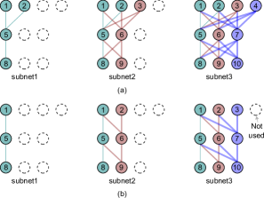
Figure 1: Structures of the slimmable network [10] and the any-width network [13]. (a) Three subnets in the slimmable network. (b) Three subnets in the any-width network.

II Background and Motivation

When neural networks are applied for inference in resource-constrained and resource-varying platforms, they should be flexible and adaptive to the varying computational resources. To achieve this goal, the slimmable network in [10] proposes to train several subnets, which share the same set of weights. When deployed into a computing system, one of the subnets is selected according to the available computational resources to provide a trade-off between accuracy and computational cost. Figure 1(a) illustrates the concept of the slimmable network, where three subnets with different numbers of weights are designed in advance. A node in this example represents either a neuron or a filter, depending whether it is a fully-connected layer or a convolutional layer. For convenience, we will refer to such a node as a neuron henceforth. In the slimmable network, the inputs to a neuron in different subnets can be different, e.g., neuron 5 in Figure 1(a). Accordingly, different batch normalization layers need to be stored for the subnets during the inference phase.

In the slimmable network, larger subnets may invalidate the computational results at neurons in a smaller subnet. Consequently, intermediate results of the smaller subnet cannot directly be reused in larger subnets. For example, in Figure 1(a), the synapse from neuron 3 to neuron 5 in subnet2 requires the recomputation of neuron 5 in subnet2 during inference. This problem is overcome in the any-width network [13], in which no synapse connects a neuron that is only in a larger subnet to another neuron in a smaller subnet, as illustrated in Figure 1(b). Accordingly, the any-width network does not require extra batch normalization layers for subnets. More importantly, the any-width network allows dynamic expansion of subnets. Once extra computational resources are available, the any-width network can always switch to the next larger subnet to enhance the inference accuracy by executing more MAC operations in the expanded network. Similarly, when the computational resources reduce dynamically, the smaller subnet can also reuse the intermediate results of the previous larger subnet.

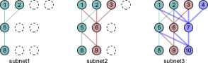
Figure 2: Structures of the proposed SteppingNet with three subnets.

Despite its advantages in dynamic subnet expansion, the any-width network still suffers from limitations. First, the structures of the subnets are manually determined. These structures must follow the regular pattern shown in Figure 1(b). This strict structural pattern, however, may impair the inference accuracy of subnets, because further potential network structures of subnets are not explored. For example, a subnet can have an irregular structure, such as subnet$1$ in Figure 2. When this subnet is expanded into subnet$2$, it only needs to be guaranteed that newly expanded neurons do not have synapses starting from them and entering the neurons in subnet$1$ to maintain the capability of dynamic subnet expansion and reduction. Second, the regular structures in the any-width network may not use up all the neurons in the neural network as shown in Figure 1(b), where neuron 4 cannot be included into a subnet if the regular structural pattern is strictly followed. Third, since the any-width network constructs the subnets according to structural rules, the computational cost in each expansion of the subnets, i.e., the extra MAC operations, is not directly controlled. Consequently, when used in computing systems with dynamically varying resources, the expansion of subnets in the any-width network may not work due to mismatch of the required and the dynamically available computational resources.

III Construction and Training of SteppingNet

To implement a series of efficient subnets whose weights are shared and whose inference accuracy is enhanced incrementally when more computational resources become available, we use the work flow shown in Figure 3. The construction process determines the structures of the subnets by moving neurons gradually between subnets. In the last step, the subnets are retrained with knowledge distillation to enhance their inference accuracy. The construction and retraining of subnets are described in detail in Section III-A and Section III-B, respectively.

III-A Constructing subnets of SteppingNet by neuron assignment

The task of subnet construction is to determine the structures of the subnets. A smaller subnet should be contained in a larger subnet so that its results can contribute to the computation results of the latter. In addition, the extra neurons in the larger subnet should not have synapses to the neurons in the smaller subnet; otherwise, the neurons in the smaller subnet need to be reevaluated, thus losing the incremental property of subnets.

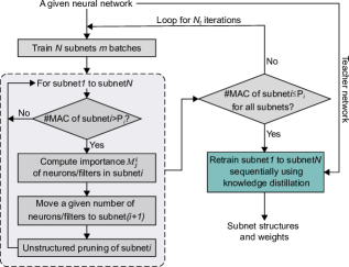
Figure 3: Work flow of SteppingNet. Except training multiple subnets with knowledge distillation in the last step, the other steps belong to subnet construction.

A straightforward idea of subnet construction is selecting weights according to their importance for each subnet. However, this method does not consider the incremental property of subnets, so that it can unfortunately block some neurons and lead to a suboptimal result. For example, in Figure 4, weights that are important for subnet1 are selected from the original network. Subnet$2$ is constructed by selecting its important weights while guaranteeing that subnet$2$ does not have synapses to the neurons in subnet$1$. After the construction of subnet$1$ and subnet$2$, all the three neurons in the second layer are already occupied by the two subnets. Therefore, it is not possible to include the remaining two neurons in the first layer into subnet$3$ without invalidating the computation results of subnet$1$ and subnet$2$. This limitation wastes the potential of neurons in subnets and thus compromises the inference accuracy of subnet$3$.

To avoid the problem above, we will evaluate the importance of the neurons with respect to all subnets and move them across subnets to gradually build up the structures of subnets while guaranteeing the incremental property. In the following, the process of moving neurons to construct subnets is described Section III-A1 and the importance evaluation of neurons is explained in Section III-A2.

III-A1 Structural construction of subnets

In SteppingNet, subnets are constructed from a given original neural network. Each subnet contains a part of the neurons and synapses of the original neural network, and a smaller subnet is completely contained in a larger subnet. The inference accuracy of the original neural network is an upper bound of the inference accuracy of the subnets.

In the construction process, the smallest subnet is first initialized with the original neural network. The neurons are gradually moved away from this subnet to fill larger subnets using the work flow in Figure 3. In this flow, the subnets are first trained for $m$ batches and their numbers of MAC operations are evaluated sequentially afterwards. If the number of MAC operations of subnet$i$ is larger than a predefined threshold $P_{i}$, some neurons in subnet$i$ are moved into subnet$(i+1)$ according to their importance to the subnets. The flow ends when the number of MAC operations of each subnet satisfies the requirement. During this process, the extra neurons in a larger subnet are not allowed to have synapses to the neurons in a smaller subnet, so that the capability of dynamic subnet expansion and reduction is maintained.

An example of the construction process is illustrated in Figure 5, where subnet$1$ is initialized using the original neural network as shown in Figure 5(a). Assume that the allowed MAC operations in the three subnets to be constructed in Figure 5 are 3, 7, 14, respectively. The number of MAC operations in subnet$1$ in Figure 5(a) thus needs to be reduced. Accordingly, neuron 4 is moved to subnet$2$ in Figure 5(b). This process is repeated for subnet$1$ and neurons gradually flow into subnet$2$. When the difference in the numbers of MAC operations of subnet$2$ and subnet$1$ is larger than $7-3=4$, the neurons start to flow from subnet$2$ to subnet$3$; Otherwise subnet$2$ cannot maintain a sufficient number of neurons, so that the number of MAC operations in subnet$2$ might be much smaller than the allowed number at the end of construction process. In Figure 5(d), the MAC difference of subnet$2$ and subnet$1$ is more than 4, so that a neuron is moved from subnet$2$ to subnet$3$ in Figure 5(e), while neuron movement from subnet$1$ to subnet$2$ is ongoing simultaneously. After the iterations in Figure 3 are finished, the structures of the subnets are determined, as illustrated in Figure 5(g).

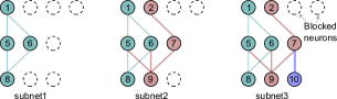
Figure 4: Inappropriate subnet construction with blocked neurons.

In moving a neuron from subnet$i$ to subnet$(i+1)$, all the synapses from this neuron to the neurons in subnet$i$ are removed to avoid the reevaluation of the neurons in subnet$i$. For example, in Figure 5(b), neuron 4 loses all the connections to the neurons in the second layer of the neural network. However, when further neurons are moved into subnet$(i+1)$, the synapses between the neurons are reestablished to maintain the inference accuracy, e.g., the synapse between neuron 4 and neuron 6 in Figure 5(c).

After neurons in the subnets are updated in an iteration, we also apply pruning [14] to remove the weights and filters that are unimportant to the inference accuracy of the corresponding subnet, such as the synapse between neuron 1 and neuron 6 and the synapse between neuron 3 and neuron 7 in Figure 5(e). Consequently, weights and the corresponding MAC operations remaining in a subnet essentially contribute to its inference accuracy. Since weights pruned in subnet$i$ may be important to larger subnets, we do not remove these weights permanently during pruning but allow them to update in the following training iterations, so that the importance of neurons to larger subnets can be evaluated correctly, as explained in Section III-A2. When a neuron with pruned weights is moved to another subnet, the corresponding synapses are revived, because these synapses may be essential to the new subnet, such as the synapse between neuron 3 and neuron 7 in Figure 5(f).

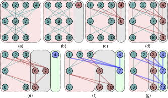
Figure 5: Subnet construction in SteppingNet. The leftmost block with neurons in green belongs to subnet$1$, the two blocks on the left with neurons in green and red (from (b) onwards) belong to subnet$2$, and the three blocks together with neurons in green, red and purple (from (e) onwards) form subnet$3$. At the beginning, subnet$1$ is initialized with the original neural network and the other subnets are empty in (a).

In the example in Figure 5, only one neuron from a subnet is moved to the next subnet in an iteration. Since the number of neurons/filters in a deep neural network can be large, in implementing SteppingNet we move multiple neurons simultaneously from a subnet to another. We first determine the number of MAC operations required to be moved from a subnet to the subsequent subnet according to the allowed number of MAC operations. Since subnet$1$ needs to move the largest number of neurons to other subnets, we use it to calculate an upper bound of the number of neurons moved between subnets in an iteration. Assume that the number of MAC operations allowed in subnet$1$ is $P_{1}$, the total number of MAC operations of the original neural network is $P_{t}$, and the total number of iterations allowed in the work flow in Figure 3 is $N_{t}$. The number of MAC operations that are moved from a subnet to the subsequent larger subnet in an iteration is then defined as $(P_{t}-P_{1})/N_{t}$ to guarantee that the final numbers of remaining MAC operations in the subnets comply with the requirements. In implementing SteppingNet, the neurons are evaluated and a set of neurons whose importance values are low and whose number of MAC operations just exceeds $(P_{t}-P_{1})/N_{t}$ are selected from subnet$i$ and moved to subnet$(i+1)$.

III-A2 Importance evaluation for neuron reallocation

In SteppingNet, if a neuron appears in subnet$i$, it also appears in all the larger subnets. The importance of this neuron with respect to different subnets may be different. Accordingly, we use a parameter $r_{j}^{i}$ to indicate the importance of the $j$th neuron with respect to subnet$i$. With $r_{j}^{i}$, we then modify the computation at the $j$th neuron in the neural network as

$$d_{j}=\varphi(r_{j}^{i}*\sum_{k=0}^{n_{j}}d_{j,k}*w_{j,k}+b_{j})$$ (1)

where $d_{j}$ is the output of this neuron. $d_{j,k}$ and $w_{j,k}$ are the input and the weight of the $k$th synapse to this neuron, respectively. $n_{j}$ is the total number of incoming synapses to this neuron. $b_{j}$ is the bias. $\varphi$ is the activation function. For CNNs, $r_{j}^{i}$ is assigned to the $j$th filter of the $i$th subnet to indicate the importance of this filter. The operation of the filter is the corresponding convolution instead of the MAC operation in (1).

During forward propagation, $r_{j}^{i}$ is set to 1 to guarantee the correct function of this neuron in inference. Since the subnets should be trained to enhance inference accuracy, we maintain a cost function $L_{i}$ for each subnet. At backward propagation, we calculate the partial derivative of the cost function $L_{i}$ to $r^{i}_{j}$ as

$$\frac{\partial L_{i}}{\partial r_{j}^{i}}=\frac{\partial L_{i}}{\partial\varphi}\frac{\partial\varphi}{\partial(r^{i}_{j}*\sum_{k=0}^{n_{j}}d_{j,k}*w_{j,k}+b_{j})}\times\sum_{k=0}^{n_{j}}d_{j,k}*w_{j,k}.$$ (2)

In backward propagation, $\frac{\partial L_{i}}{\partial r_{j}^{i}}$ is a floating-point number, which we use to make the binary decision whether a neuron should be moved to the next larger subnet.

In selecting a neuron to move from subnet$i$ to subnet$(i+1)$, $\frac{\partial L_{i}}{\partial r_{j}^{i}}$ does not provide a sufficiently good indication, since a neuron in subnet$i$ is also contained in all the subnets larger than subnet$i$. Accordingly, we tend to keep the neurons that are also important to all the larger subnets, and define the selection criterion for the $j$th neuron in the $i$th subnet as

$$M^{i}_{j}=\sum_{k=i}^{N}\alpha_{k}\left|\frac{\partial L_{k}}{\partial r_{j}^{k}}\right|$$ (3)

where $\alpha_{k}$ is a constant defining the contribution ratio of $\frac{\partial L_{k}}{\partial r_{j}^{k}}$ of a neuron with respect to subnet$k$. $N$ is the number of subnets. In an iteration, after $M^{i}_{j}$ are updated, the neurons with the smallest $M^{i}_{j}$ are moved to the next subnet.

TABLE I: Results of SteppingNet

Test cases			Orig. Net		Subnet1			Subnet2			Subnet3			Subnet4
Network	Dataset		Acc.		$A_{1}$	$M_{1}/M_{t}$		$A_{2}$	$M_{2}/M_{t}$		$A_{3}$	$M_{3}/M_{t}$		$A_{4}$	$M_{4}/M_{t}$
LeNet-3C1L	Cifar10		83.36%		68.5%	9.65%		77.38%	29.55%		79.81%	48.62%		80.4%	78.52%
LeNet-5	Cifar10		74.96%		51.8%	13.64%		59.56%	26.54%		68.64%	55.07%		72.03%	82.74%
VGG-16	Cifar100		70.32%		63.26%	15.97%		68.19%	32.54%		68.19%	47.39%		68.14%	67.78%

Because moving neurons between subnets changes the structures as well as the cost functions of the subsets, we train the subnets with $m$ batches before evaluating the neurons using (3), as shown in Figure 3. In this process, the training of a larger subnet also updates the weights in smaller subnets, whose values have been determined by directly training the smaller subnets themselves in the same iteration. Consequently, the accuracy of smaller subnets may degrade after a larger subnet is trained. To reduce the effect of updating weights in smaller subnets when training a larger subnet, we decrease the learning rate of weights in a smaller subnet by the ratio $\beta^{(j-i)}$, where $\beta$ is a constant between 0 and 1 and $j$ and $i$ are the indexes of the larger and the smaller subnets, respectively. $(j-i)$ is used as the exponent of $\beta$ so that the smaller the subnets are, the more their learning rates are decreased. With this reduction of learning rates, smaller subnets obtain more stability to maintain their inference accuracy when larger subnets are trained.

III-B Retraining subnets with knowledge distillation

After subnets are constructed with the method in Section III-A, we retrain them to improve their inference accuracy with knowledge distillation [15]. In this retraining, the teacher network is the original neural network from which subnets are constructed. This neural network has a high accuracy compared with the subnets, which are the student networks, so that it is used to guide the subnets during retraining.

When retraining a subnet, we modify its cost function as follows

$$L_{i}^{\prime} =\gamma\times L_{i}+(1-\gamma)\sum_{k=1}^{n_{c}}Y_{k}log(\frac{Y_{k}^{pre}}{Y_{k}})$$ (4)

where $L_{i}$ is the cross entropy of subnet$i$. $\sum_{k=1}^{n_{c}}Y_{k}log(\frac{Y_{k}^{pre}}{Y_{k}})$ is the Kullback-Leibler divergence [16] of subnet$i$ to the pretrained original neural network, where $Y^{pre}_{k}$ and $Y_{k}$ are the $k$th outputs of the original neural network and subnet$i$, respectively. $n_{c}$ is the number of output classes. $\gamma$ is a constant between 0 and 1 to adjust the priority of Kullback-Leibler divergence in (4). The smaller the difference between $Y_{k}^{pre}$ and $Y_{k}$ is, the more similar results the subnets generate compared with the original neural network.

In the retraining phase, we train the subnets in an ascending order in each epoch using the modified cost function in (4). During this training, we also reduce the learning rates of subnets as described in Section III-A2 to avoid drastic weight change in smaller subnets. With this multi-subnet knowledge distillation, the inference accuracy of all these subnets can be enhanced and balanced as a whole.

IV Experimental Results

To evaluate the effectiveness of SteppingNet, three neural networks, LeNet-3C1L, LeNet-5 and VGG-16 were applied onto two datasets, Cifar10 and Cifar100, respectively. as shown in the first two columns of Table I. The construction of subnets and their retraining were implemented using PyTorch and tested on Nvidia Quadro RTX 6000 GPUs.

To demonstrate that SteppingNet provides an incremental accuracy improvement with respect to computational resources, four subnets were constructed and retrained with the framework described in Section III. During this construction, the connections from new neurons in a subnet to the neurons in the previous smaller subnets were prohibited to enable computational reuse as described in Section III. To provide the construction process more flexibility, we expanded the number of neurons/filters of each layer in the original network as in [13] and initialized the first subnet in the construction process with this expanded network. For LeNet-3C1L, LeNet-5, and VGG-16, the corresponding expansion ratios were set to 1.8, 2.0, 1.8, respectively. For example, in the expanded LeNet-3C1L, the number of neurons/filters is 1.8 times of that of the original network.

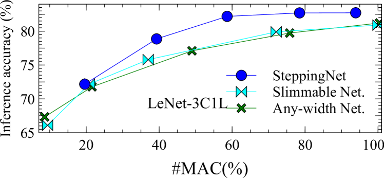
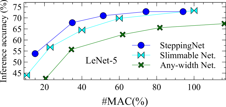
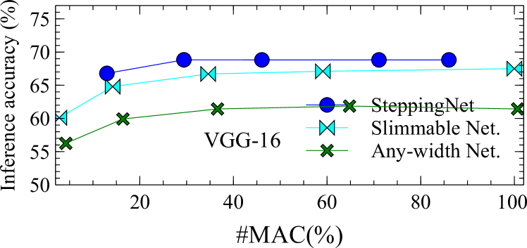
Figure 6: Comparison with the any-width network and the slimmable network.

In the flow in Figure 3, we set the number of training batches at the beginning of each iteration to 250, 250, and 100 for LeNet-3C1L, LeNet-5, and VGG-16, respectively. The total number of allowed iterations $N_{t}$ was set to 300. The weight threshold in the unstructured pruning was set to $1\times 10^{-5}$. The coefficients $\alpha_{k}$ in (3) were increased to 1.5 times from $\alpha_{1}=1$ for each larger subnet to emphasize the importance of the neurons to these larger subnets, so that the neurons remaining in the current subnet also make good contribution to the inference accuracy of the larger subnets. $\beta$ in weight update suppression in Section III-A2 was set to 0.9. $\gamma$ in (4) was set to 0.4 to balance the cross entropy and the effect of knowledge distillation in retraining.

During subnet construction and retraining, the inference accuracy of the largest subnet could not be improved further after a certain number of MAC operations was reached. For example, in LeNet-3C1L and LeNet-5, after executing around 85% MAC operations of the original network, the inference accuracy of the largest subnet reached more than 95% of the inference accuracy of the original network and did not increase any further. For VGG-16, this threshold was around 70%. Accordingly, we set these numbers of MAC operations as the resources allowed in the largest subnets and decreased from these numbers to set the resources allowed in smaller subnets, so that the subnets can produce inference accuracy at different levels of MAC operations. For the three neural networks, LeNet-3C1L, LeNet-5 and VGG-16, the allowed MAC operations in the four subnets were then set to 10%/30%/50%/85%, 15%/30%/60%/85%, 20%/40%/50%/70% of the original neural networks, respectively.

Table I shows the inference accuracy of the test cases. The third column shows the inference accuracy of the original neural networks. The columns $A_{1}$, $A_{2}$, $A_{3}$, and $A_{4}$ show the inference accuracy of the subnets. The columns $M_{1}/M_{t}$, $M_{2}/M_{t}$, $M_{3}/M_{t}$ and $M_{4}/M_{t}$ show the percentages of MAC operations in the subnets with respect to the number of MAC operations $M_{t}$ of the original neural network. According to this table, it can be observed that the inference accuracy of subnets was improved by more MAC operations. In addition, the incremental accuracy enhancement was not necessarily linear with respect to the number of MAC operations. For example, with even about 10% of the total number of MAC operations, the inference accuracy of LeNet-3C1L can already reach 68.5%, which is important for some scenarios, e.g., autonomous driving, to make a preliminary decision. The inference accuracy of the largest subnets was already close to that of the original neural networks, and the difference was to provide the property of incremental enhancement.

To demonstrate the performance of SteppingNet compared with the any-width network [13] and the slimmable network[10], we executed the any-width network and the slimmable network on the three networks in Table I to obtain the inference accuracy of five subnets under various numbers of MAC operations. The accuracy comparison is illustrated in Figure 6. This comparison demonstrates that SteppingNet outperforms the any-width network and the slimmable network in inference accuracy under the same numbers of MAC operations, due to the fact that SteppingNet enables more flexible subnet structures than the any-width network and the slimmable network.

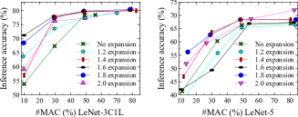
Figure 7: Accuracy comparison with different expansion ratios.

Before subnet construction, we expanded the number of neurons/filters in the original network with a given ratio to allow more flexible subnet structures to be identified. To demonstrate how this ratio affects the inference accuracy, we changed these ratios and tested the inference accuracy of the constructed subnets, as shown in Figure 7, where the ratio of MAC operations is with respect to the number of the MAC operations of the original neural network without expansion. According to this figure, it can be seen that different expansion ratios do affect the accuracy of the subnets due to more available subnet structures. The ratios that provide the best overall accuracy were selected to generate the results in Table I.

During the construction of subnets, we suppressed the update of weights in smaller subnets to avoid accuracy loss when larger subnets were trained, as described in Section III-A2. After subnet construction, we adopted knowledge distillation to retrain the subnets. To demonstrate the effectiveness of these techniques, we compared the inference accuracy with these techniques disabled individually. The results are shown in Figure 8. According to this figure, both weight update suppression and knowledge distillation contribute to the inference accuracy. When these two techniques are combined, inference accuracy of many subnets, especially the smaller ones, can be enhanced. For larger subnets, these techniques may interfere with each other and lead to slight accuracy fluctuation, but the overall accuracy still stays relatively stable.

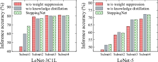
Figure 8: Accuracy comparison with and without suppression of weight update and knowledge distillation.

V Conclusion

In this paper, we have proposed a design scheme, called SteppingNet, for neural networks executed on resource-constrained and resource-varying platforms. SteppingNet constructs a series of subnets with different numbers of MAC operations and the intermediate results of smaller subnets in SteppingNet can be reused directly in subsequent larger subnets. Experimental results demonstrated that SteppingNet outperforms state-of-the-art work in inference accuracy under the same limit of computational resources.

References

- [1] K. He, X. Zhang, S. Ren, and J. Sun, “Deep residual learning for image recognition,” in IEEE Conf. Comput. Vis. Patt. Recog. (CVPR), 2016.
- [2] J. Kocić, N. Jovičić, and V. Drndarević, “An end-to-end deep neural network for autonomous driving designed for embedded automotive platforms,” Sensors, vol. 19, no. 9, 2019.
- [3] S.-C. Lin, Y. Zhang, C.-H. Hsu, M. Skach, M. E. Haque, L. Tang, and J. Mars, “The architectural implications of autonomous driving: Constraints and acceleration,” in International Conference on Architectural Support for Programming Languages and Operating Systems, 2018.
- [4] S. C. Jha, A. T. Koc, R. Vannithamby, and M. Torlak, “Adaptive DRX configuration to optimize device power saving and latency of mobile applications over LTE advanced network,” in IEEE Int. Conf. on Comm., 2013.
- [5] A. G. Howard, M. Zhu, B. Chen, D. Kalenichenko, W. Wang, T. Weyand, M. Andreetto, and H. Adam, “MobileNets: Efficient convolutional neural networks for mobile vision applications,” CoRR, vol. abs/1704.04861, 2017.
- [6] A. Howard, A. Zhmoginov, L.-C. Chen, M. Sandler, and M. Zhu, “Inverted residuals and linear bottlenecks: Mobile networks for classification, detection and segmentation,” in IEEE Conf. Comput. Vis. Patt. Recog. (CVPR), 2018.
- [7] X. Zhang, X. Zhou, M. Lin, and J. Sun, “ShuffleNet: An extremely efficient convolutional neural network for mobile devices,” CoRR, vol. abs/1707.01083, 2017.
- [8] H. Cai, C. Gan, T. Wang, Z. Zhang, and S. Han, “Once-for-All: Train one network and specilize it for efficient deployment,” in Int. Conf. Learn. Repr. (ICLR), 2020.
- [9] E. Kim, C. Ahn, and S. Oh, “NestedNet: Learning nested sparse structures in deep neural networks,” in IEEE Conf. Comput. Vis. Patt. Recog. (CVPR), 2018.
- [10] J. Yu, L. Yang, N. Xu, J. Yang, and T. Huang, “Slimmable neural networks,” in Int. Conf. Learn. Repr. (ICLR), 2019.
- [11] J. Yu and T. Huang, “Universally slimmable networks and improved training techniques,” in IEEE/CVF Int. Conf. Comp. Vision (ICCV), 2019.
- [12] G. Huang, D. Chen, T. Li, F. Wu, L. van der Maaten, and K. Q. Weinberger, “Multi-scale dense networks for resource efficient image classification,” in ICLR, 2018.
- [13] T. Vu, M. Eder, T. Price, and J.-M. Frahm, “Any-width networks,” in IEEE Conf. Comput. Vis. Patt. Recog. (CVPR), 2020.
- [14] S. Han, H. Mao, and W. J. Dally, “Deep Compression: Compressing deep neural network with pruning, trained quantization and huffman coding,” in Int. Conf. Learn. Repr. (ICLR), 2016.
- [15] Y. Zhang, T. Xiang, T. M. Hospedales, and H. Lu, “Deep mutual learning,” in IEEE Conf. Comput. Vis. Patt. Recog. (CVPR), 2018.
- [16] J. M. Joyce, Kullback-Leibler Divergence. Springer Berlin Heidelberg, 2011.