CorrectNet: Robustness Enhancement of Analog In-Memory Computing for Neural Networks by Error Suppression and Compensation

Abstract

The last decade has witnessed the breakthrough of deep neural networks (DNNs) in many fields. With the increasing depth of DNNs, hundreds of millions of multiply-and-accumulate (MAC) operations need to be executed. To accelerate such operations efficiently, analog in-memory computing platforms based on emerging devices, e.g., resistive RAM (RRAM), have been introduced. These acceleration platforms rely on analog properties of the devices and thus suffer from process variations and noise. Consequently, weights in neural networks configured into these platforms can deviate from the expected values, which may lead to feature errors and a significant degradation of inference accuracy. To address this issue, in this paper, we propose a framework to enhance the robustness of neural networks under variations and noise. First, a modified Lipschitz constant regularization is proposed during neural network training to suppress the amplification of errors propagated through network layers. Afterwards, error compensation is introduced at necessary locations determined by reinforcement learning to rescue the feature maps with remaining errors. Experimental results demonstrate that inference accuracy of neural networks can be recovered from as low as 1.69% under variations and noise back to more than 95% of their original accuracy, while the training and hardware cost are negligible.

I Introduction

Deep neural networks (DNNs) have been applied successfully in many fields, e.g., image recognition [1] and language processing [2]. DNNs achieve their accuracy using a large number of layers [3]. This results in tens of millions weights and hundreds of millions of multiply-and-accumulate (MAC) operations in a neural network. To accelerate these operations, analog in-memory computing platforms based on emerging technologies, e.g., resistive RAM (RRAM) [4, 5], have been introduced. In such platforms, MAC operations are implemented by analog devices based on Ohm’s law and Kirchhoff’s current law, so that a high computation and energy efficiency can be achieved.

These analog-based computing platforms, however, suffer from manufacturing process variations and noise [6]. Accordingly, inference accuracy of neural networks implemented with such platforms may degrade significantly in practice. For example, in an RRAM-based computing platform, RRAM cells should be programmed to specific conductances to represent weights of neural networks. However, variations of physical parameters of RRAM cells, e.g., cross-section area, cause variability in their electrical properties. Accordingly, when a programming voltage is applied onto an RRAM cell, the resulting conductance value under process variations and noise deviates from the nominal value. Consequently, weights in neural networks may not be reflected accurately, and the feature maps at the output of layers can become erroneous. When such incorrect feature maps travel through subsequent layers with deviated weights, the errors can be amplified, which results in a significant degradation of inference accuracy and thus offsets the advantages of these platforms in computation and energy efficiency [7].

Several previous approaches have been proposed to tackle the accuracy degradation problem due to hardware uncertainty. The method in [8] applies knowledge distillation to train a variation-aware model and replicates some important weights into SRAM cells to enhance computational robustness. Similarly, [9] randomly selects some weights and maps them into on-chip memory for further training to improve accuracy. However, these methods still require online retraining to restore the inference accuracy, which incurs extra training and test cost. Trying to adjust weights to absorb the effect of variations, [7] proposes a variation-aware training approach by compensating the impact of device variations and including it in the loss function. The methods in [10, 11] train neural networks statistically by directly modeling variations as functions of random variables. [12] follows a similar approach regarding variation-aware mapping which represents large weights by RRAM cells with lower variations in the crossbar and trains the neural network adaptively online. Such approaches, however, either need prior knowledge of the variation profile, which requires testing and measurement of each manufactured chip, or are limited to neural networks with only a small depth.

Different from the approaches above, in this paper, we introduce a method to mitigate the effects of weight variations and noise in analog in-memory computing platforms by two techniques: error suppression and error compensation. The key contributions of this work are summarized as follows:

• Error suppression is realized by training neural networks under modified Lipschitz constant regularization, so that weight variations do not cause the amplification of errors resulting from previous layers.

• Error compensation is introduced to recover feature maps from potential errors. The locations of error compensation and the number of filters for compensation are determined by reinforcement learning to achieve a balance between accuracy recovery and computational cost.

• Experimental results demonstrate that the inference accuracy of neural networks can be recovered from as low as 1.69% under variations and noise back to more than 95% of their original accuracy, while the training and hardware cost are negligible.

The rest of this paper is organized as follows. In Section II, we explain the background and motivation of this work. In Section III, we introduce the techniques of error suppression by Lipschitz constant regularization and error compensation for sensitive layers. Experimental results are reported in Section IV and conclusions are drawn in Section V.

II Preliminaries and motivation

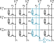
Figure 1: The structure of RRAM crossbar.

To accelerate DNNs, emerging platforms with analog devices, e.g., RRAM, have a huge advantage in computation and energy efficiency. Figure 1 illustrates the structure of an RRAM-based crossbar, where RRAM cells sit at the crossing points and transistors are used to enable RRAM cells. To implement MAC operations, RRAM cells are first programmed to the target conductance values to represent weights of DNNs. Afterwards, voltages are applied on the horizontal wordlines while voltages on the vertical bitlines are connected to ground. The resulting current in an RRAM cell is thus the multiplication result of the voltage and its conductance. The accumulated currents at the bottom of each column is the addition result.

Analog accelerators, however, are inherently susceptible to variations and noise from manufacturing process and operation environments, respectively. These variations and noise cause the programmed conductances to deviate from the target values. Accordingly, weights of neural networks represented by conductances of RRAM cells vary from their nominal values, leading to a degradation of inference accuracy.

To demonstrate the effect of variations and noise on the inference accuracy of neural networks, we use a log-normal distribution to inject variations into weights of neural networks as an example. This log-normal variation model is widely adopted, e.g., in [11, 12, 7].

$$w =w_{nominal}*e^{\theta}$$ (1)

$$\theta \sim N(0,\sigma^{2})$$ (2)

where $w_{nominal}$ is the nominal value of a weight after training and $\theta$ is a Gaussian random variable with $\sigma$ as its standard deviation. For different weights, their corresponding variables $\theta$s are independent.

Figure 2 shows the mean values and the standard deviations of the inference accuracy of VGG16 [13] and LeNet-5 [14] on Cifar100, Cifar10, and MNIST datasets under different levels of weight variations using the model in (1) and (2). The solid lines in the middle of the ranges represent the mean values and the ranges represent the standard deviations. According to Figure 2, even with relatively small variations, the accuracies of the neural networks have degraded noticeably. As the amount of variations increases, the accuracy drops even more drastically, which makes the neural networks unusable in practice. In addition, VGG16 with more layers exhibited a more drastic accuracy degradation than LeNet-5. The reason is that as these data propagate through more layers, not only are further variations accumulated but the deviations in early layers can also be amplified by the computation in later layers.

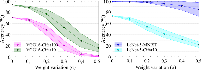
Figure 2: Inference accuracy degradation of neural networks under variations in weights.

III Design methodology for error suppression and compensation

In this paper, we propose to suppress error propagation through layers by applying a modified Lipschitz constant regularization [15, 16, 17]. To further enhance inference accuracy, an error compensation for selected layers is proposed. With these techniques, the inference accuracy of neural networks can be recovered effectively to enable their execution on analog accelerators for energy-efficient computing. The proposed method is very general and can be applied into any analog in-memory computing platform for neural networks by adapting the variation model according to the corresponding analog devices.

III-A Lipschitz constant regularization for error suppression

A function $f:X\rightarrow Y$ is Lipschitz constrained [16, 15] if it satisfies a certain p-distance metric

$$\left|f(\mathbf{x_{1}})-f(\mathbf{x_{2}})\right|_{p}\leq k\left|\mathbf{x_{1}-x_{2}}\right|_{p},\;\;\forall\mathbf{x_{1},x_{2}}\in X$$ (3)

where the p-norm $\left|\cdot\right|_{p}$ calculates the p-distance metric between two vectors. For the function $f$, the smallest value of the non-negative constant $k$ is denoted as the Lipschitz constant $L(f)=k$ and $f$ is said to be k-Lipschitz. The Lipschitz constant $L(f)$ describes how $f$ scales with respect to its input. If $L(f)$ is larger than 1, any change in the input is amplified by $f$; otherwise, the change is suppressed. For multiple functions $f_{1},\dots f_{l}$ with Lipschitz constants $k_{1},\cdots k_{l}$, their composition is also Lipschitz constrained as

$$f=(f_{l}\circ f_{l-1}\circ...\circ f_{1})(x)$$ (4)

$$L(f)\leq k_{l}\cdot k_{l-1}\cdot...\cdot k_{1}.$$ (5)

In other words, the Lipschitz constant of the composition function is upper bounded by $k_{l}\cdot k_{l-1}\cdot...\cdot k_{1}$.

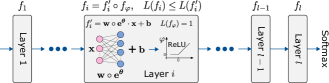
Figure 3: Lipschitz constant regularization and composition in a neural network.

The composition of functions and the Lipschitz constant of the composition can be used to bound the forward propagation of errors in a neural network, because forward propagation of a neural network can be considered as a composition of operations of successive layers, as shown in Figure 3. If the $i$th layer of a neural network realizes a function $f_{i}(\mathbf{x})$, the function of the neural network with $l$ layers can thus be written as (4).

The concept of suppressing errors in neural networks can be illustrated in Figure 4. When specific data, e.g., an image, travels through the neural network, the inputs to the $i$th layer may differ from the nominal values, because the variations in the weights of the first $i-1$ layers cause changes in their outputs and thus in the inputs of the $i$th layer. The task of error suppression is thus to train the neural network to obtain a set of weights that limit the deviation of the outputs of layers of the neural network from their nominal values when variations are considered. This training is implemented based on the composition of the functions of the layers in the neural network and Lipschitz constant regularization.

Assume that the nominal inputs to the $i$th layer are written as $\mathbf{x_{1}}$ and the inputs affected by variations in the first $i-1$ layers are written as $\mathbf{x_{2}}$, then the deviation of the outputs of the $i$th layer from the nominal values can be evaluated as $\left|f_{i}(\mathbf{x_{1}})-f_{i}(\mathbf{x_{2}})\right|_{p}$, where $f_{i}(\cdot)$ is the function of the $i$th layer converting its inputs to the outputs. To suppress this deviation, called error henceforth, we will use (3) with $k\leq 1$. In other words, errors will not be amplified after a layer is traveled through. According to the composition in (4), if all the layers in the neural network can meet the Lipschitz constraint with $k\leq 1$, the errors at the outputs of the neural network will also be restrained according to (5).

For a specific layer in the neural network, its function $f_{i}$ can be expressed as the composition of $f_{i}^{\prime}$ and $f_{\varphi}$, as illustrated in Figure 3. $f_{i}^{\prime}=\mathbf{w\circ e^{\boldsymbol{\theta}}\cdot\mathbf{x}}+\mathbf{b}$ implements the matrix-vector multiplication and the sum with bias, in which $\mathbf{b}$ is the bias vector and $\mathbf{w}$ is the weight matrix of the layer. $\mathbf{w\circ e^{\boldsymbol{\theta}}}$ is the element-wise multiplication of the weight values with the random variables $\mathbf{e^{\boldsymbol{\theta}}}$ to incorporate the effect of variations according to (1). $f_{\varphi}$ is the ReLU function. The ReLU function does not amplify any deviations and its Lipschitz constant is always equal to 1. Therefore, we only need to constrain the Lipschitz constant of $f_{i}^{\prime}$ to suppress error amplification, as

$$\left|(\mathbf{w\circ e^{\boldsymbol{\theta}}\cdot\mathbf{x_{1}}}+\mathbf{b})-(\mathbf{w\circ e^{\boldsymbol{\theta}}\cdot\mathbf{x_{2}}}+\mathbf{b})\right|_{p} \leq\;k\left|\mathbf{x_{1}}-\mathbf{x_{2}}\right|_{p}$$ (6)

$$\Leftrightarrow\;\left|\mathbf{w\circ e^{\boldsymbol{\theta}}}\cdot(\mathbf{x_{1}}-\mathbf{x_{2}})\right|_{p} \leq\;k\left|\mathbf{x_{1}}-\mathbf{x_{2}}\right|_{p}$$ (7)

$$\Leftrightarrow\frac{\left|\mathbf{w\circ e^{\boldsymbol{\theta}}}\cdot(\mathbf{x_{1}}-\mathbf{x_{2}})\right|_{p}}{\left|\mathbf{x_{1}}-\mathbf{x_{2}}\right|_{p}} \leq\;k.$$ (8)

According to the definition of the p-norm of a matrix $\parallel.\parallel_{p}$, the condition in (8) can be expressed further as

$$sup\left(\frac{\left|\mathbf{w\circ e^{\boldsymbol{\theta}}}\cdot(\mathbf{x_{1}}-\mathbf{x_{2}})\right|_{p}}{\left|\mathbf{x_{1}}-\mathbf{x_{2}}\right|_{p}}\right)=\parallel\mathbf{w\circ e^{\boldsymbol{\theta}}}\parallel_{p}\leq k$$ (9)

which shows that error propagation in a layer can be suppressed by constraining $\parallel\mathbf{w\cdot e^{\boldsymbol{\theta}}}\parallel_{p}$.

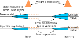
Figure 4: Lipschitz constant regularization for error suppression.

Since $\boldsymbol{e^{\theta}}$ in (9) represents a matrix of independent random variations, $\parallel\mathbf{w\circ e^{\boldsymbol{\theta}}}\parallel_{p}$ cannot be evaluated directly. To address this problem, we use ${\mu_{e^{\theta}}+3\cdot\sigma_{e^{\theta}}}$ to bound the random variable ${e^{\theta}}$. Since ${e^{\theta}}$ has a lognormal distribution, ${\mu_{e^{\theta}}+3\cdot\sigma_{e^{\theta}}}=e^{\frac{\sigma^{2}}{2}}+3\sqrt{(e^{\sigma^{2}}-1)e^{\sigma^{2}}}$, in which $\sigma$ is the standard deviation of $\theta$. Accordingly, (9) can be converted into

$$\parallel\mathbf{w}\parallel_{p}\leq\lambda,\;\;\lambda=\frac{k}{e^{\frac{\sigma^{2}}{2}}+3\sqrt{(e^{\sigma^{2}}-1)e^{\sigma^{2}}}}.$$ (10)

In the proposed method, we use the $L^{2}$ norm to bound $\mathbf{w}$ in (10), which corresponds to the spectral norm of $\mathbf{w}$. The spectral norm of a matrix is the maximum singular value of the matrix. To limit the spectral norm of the weight matrix, a regularization term is added to the loss function when training the neural network, as

$$Loss=L_{ce}+\beta*\sum_{\mathbf{w_{i}}\in\mathbf{W}}\parallel\mathbf{w_{i}^{T}w_{i}}-\lambda^{2}\mathbf{I}\parallel^{2}$$ (11)

where $L_{ce}$ is the original cross-entropy loss and $\mathbf{w_{i}}$ is the weight matrix of the $i$th layer, $\mathbf{W}$ is the set of weight matrices of all layers, and $\beta$ is a regularization hyperparameter. The added regularization term keeps the weight matrix orthogonal to limit its maximum singular value by $\lambda$ and hence limit its spectral norm.

The extra regularization term in (11) is calculated from all the layers in the neural network. In applying (11), $\lambda$ is determined by setting the Lipschitz constant $k$ to 1, so that errors will not be amplified. According to (4) and (5), this composition can thus suppress error propagation in the whole neural network.

III-B Error compensation for accuracy recovery

To further enhance inference accuracy, we propose to introduce light-weighted error compensation to the early layers to recover the inference accuracy. This error compensation incurs only a marginal computational cost, so that it can be executed on digital circuits [18] and is thus considered immune from the effect of variations.

Inspired by the concept of error correction in communication systems, which has been proposed as early as in [19], we generate error compensation data from the input and the output of a layer. The error compensation data are then used by a compensator to reduce the errors propagated through this layer. The concept of applying error compensation to a convolutional layer in a neural network is illustrated in Figure 5. The generator is a small convolutional layer. The input and output feature maps of the original convolutional layer (conv1) are concatenated and used as the input of the generator to produce the compensation data. Since the dimensions of input feature maps and output features maps of the original layer do not match, we apply average pooling to reduce the dimension of the input feature maps so that they can be concatenated with the output feature maps and processed by the same filter.

The generator contains $m$ $1\times 1\times(l+n)$ filters, where $l$ and $n$ are the number of input feature maps and the number of output feature maps in the original layer (conv1), respectively. In the example in Figure 5, we use $l=n=3$ to explain the working mechanism of the generator. We use 1$\times$1 kernel dimension for two advantages. First, its computational overhead is low. Second, the generated compensation data has the same dimension of the output feature maps of the original layer, so that error compensation can also be implemented with simple $1\times 1$ kernels in the compensator. The number of filters $m$ indicates the number of output feature maps produced by the generator, e.g., 3 in Figure 5. The larger $m$ is, the larger is the computational cost and the more robust the neural network potentially becomes.

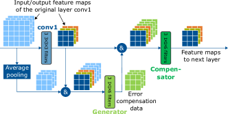
Figure 5: Error compensation for a convolutional layer.

The compensator is also a convolutional layer taking the compensation data generated by the generator and the output feature maps of the original layer as input. This compensator contains $n$ $1\times 1\times(n+m)$ filters. The $n$ filters in the compensator guarantee that the compensator produces the same number of feature maps as the original layer. The $n+m$ kernels are required due to the concatenation of the output feature maps of the original layer and the outputs of the generator.

When training the weights in the generators and compensators introduced to some layers in a neural network, the weights in the original layers are fixed to the values after applying Lipschitz constant regularization and stay non-trainable, while the weights in the generators and compensators are kept trainable. The generators and compensators are then trained with the same training data using the original cost function. In this training, variations are sampled statistically and applied to the corresponding weight values in the original layer during each training batch. The weights in the generators and compensators are then adjusted in backward propagation to reduce the cost function.

To determine the locations of error compensation, we first inject variations into the layers from the last one backwards to the $i$th layer. When $i$ is reduced, more layers contain variations, leading to a decreased inference accuracy. The candidates of the neural network layers for error compensation are then determined as the first $i$ layers when the variations in the $i$th layer to the last layer lead to an inference accuracy lower than 95% of the original accuracy.

In the next step, we will apply RL to select concrete layers in the first $i$ layers and their numbers of filters for error compensation. During this process all the layers of a neural network are injected variations. Figure 6 illustrates the application of RL, where the environment is defined as the neural network trained with error suppression and compensation whose locations and the filter numbers are determined by RL. The state of the environment is the specified locations of error compensation and the corresponding number of filters. To represent the state, we use a sequence of $n$ floating point numbers, e.g., $S_{1}$, …, $S_{i}$, … $S_{n}$, where $S_{i}$ is the ratio of the number of filters in the generator to the number of filters in the original $i$th layer. For example, $S_{2}=0.5$ means that the number of filters in the corresponding generator of the second layer is 0.5 times the number of filters of the original second layer. $S\leq 0$ means no insertion of error compensation at a layer. To generate such a sequence for the environment state, we adopt recurrent neural network as the policy neural network in the agent.

To train the policy neural network, we define a reward function as follows

$$R=\begin{cases}acc_{avg}-acc_{std}-overhead,&\text{if }overhead\leq limit\\ -overhead,&\text{otherwise}\end{cases}$$ (12)

where $acc_{avg}$, and $acc_{std}$ are the average and the standard deviations of the inference accuracy of the trained neural network under the current environment state, respectively. The overhead represents the ratio of the number of weights in the compensation layers to the number of weights in the original neural network. To avoid large computational cost incurred by error compensation during the search process, a maximum number of weights for error compensation is set. If the overhead of a solution exceeds the maximum limit in (12), a negative reward is generated directly, so that the training of neural networks with error suppression and compensation in the current iteration can be skipped to make the agent learn fast and thus reduce execution time. In the experiments, 1%, 2%, and 3% weight overhead were used as the maximum limit and the solution that generates the best accuracy was selected as the result. To determine the parameters of the policy neural network, a given number of episodes, each of which includes a specific number of learning iterations, are used.

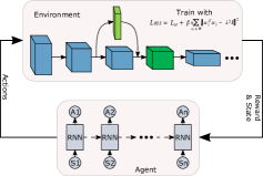
Figure 6: RL search for locations and filter numbers of error compensation. $A_{1}$, $A_{2}$, … $A_{n}$ is the action sequence generated by the policy neural network in the agent. $S_{1}$, $S_{2}$, … $S_{n}$ is the sequence to represent the state of the environment.

IV Experimental results

To evaluate the proposed framework, two neural networks, VGG16 [13] and LeNet-5 [14] were tested against three different datasets, Cifar100, Cifar10 and MNIST. The neural networks were trained with Nvidia Quadro RTX 6000 GPUs. The variation model used in the experiments was the log-normal distribution of weights mapped onto RRAM cells (1) and (2) as in [11, 12, 7]. In (10) and (11), $k$ is set to 1 to suppress the propagation of errors and $\lambda$ is determined based on the variations and the value of $k$. In the experiments, the network weights were sampled 250 times according to the variation model in (1) and (2) and inference accuracy was evaluated for each sample.

Table I summarizes the results showing the performance of the CorrectNet framework when $\sigma$ in (1) and (2) was set to 0.5. This variation setting is already very large for variations in RRAM cells [11, 12, 7]. The column $\sigma=0$ in Table I shows the inference accuracy of the original neural networks without variations. When variations of the amount $\sigma=0.5$ were applied to the weights in the original neural networks, the inference accuracy degraded significantly down to as low as 1.69% on average for VGG16-Cifar100. With the CorrectNet framework, this accuracy can be recovered back to 67.01% on average, more than 95% of the inference accuracy without variations. In Table I, the lowest ratio of the inference accuracy of CorrectNet to the original inference accuracy without variation is 92% (LeNet-5-Cifar10, 74.9%/80.89%=92.6%).

In the CorrectNet framework, the Lipschitz training method does not require extra resource or incur extra computational cost. The overhead results from the compensation layers. In Table I, the weight overhead is calculated as the percentage of the number of weights in the compensation layers to the number of weights in the original neural network. Compared with the computational operations in the original neural networks, the weight overhead of CorrectNet is marginal while an effective accuracy recovery is still achieved. The numbers of compensation layers in the neural networks after applying CorrectNet are also shown in the last column of Table I, which confirm that only some layers in the original neural networks require error compensation after error suppression with Lipschitz constant regularization is applied.

TABLE I: Experimental results of CorrectNet.

Network-Dataset		Inference accuracy					CorrectNet
		Original network			CorrectNet		overhead
		$\sigma=0$	$\sigma=0.5$		$\sigma=0.5$		Weights	#Layers
VGG16-Cifar100		70.52%	1.69%		67.01%		1.03%	4
VGG16-Cifar10		93.2%	16.01%		91.29%		0.58%	3
LeNet-5-Cifar10		80.89%	25.29%		74.9%		3.47%	1
LeNet-5-MNIST		98.79%	84.58%		97.47%		5%	2

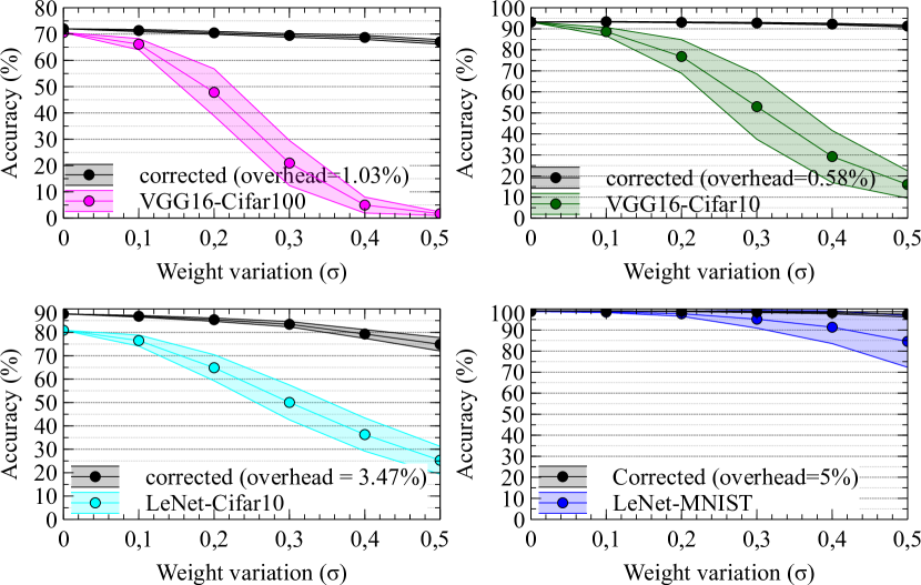
Figure 7: Accuracy of CorrectNet under different variations.

To demonstrate the capability of CorrectNet under different variation scenarios, we tested this framework using the same combinations of neural networks and datasets under different variation settings. The results are shown in Figure 7. In each of these figures, we compare the inference accuracy of CorrectNet and the original neural network. The mean values are shown with the solid lines while the ranges show the standard deviations. In all these test cases, CorrectNet has demonstrated an effective and robust trend to recover inference accuracy under different variations.

To evaluate CorrectNet, we also compare its results with those from [9, 8, 11] as shown in Figure 8. The x-axis represents the overhead incurred by weights for error compensation, and the y-axis is the mean value of the inference accuracy under variations of $\sigma=0.5$. According to this comparison, CorrectNet achieves a higher accuracy than [8] and [9] with a smaller overhead in case of non-online retraining. In the case with time-consuming online retraining in [8] and [9], CorrectNet can also achieve a similar accuracy with a lower overhead while time-consuming online retraining is not needed. CorrectNet also outperforms [11] in accuracy with a slightly larger overhead.

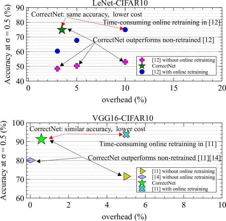
Figure 8: CorrectNet versus the state of the art [9, 8, 11].

To demonstrate the effectiveness of Lipschitz constant regularization, we added variations to the weights from the $i$th layer to the last layer of the neural networks after training with this regularization, while error compensation was disabled. Figure 9 shows the inference accuracy of the neural networks with these variations from the $i$th layer to the last layer while $\sigma$ was set to 0.5. The results corresponding to starting layer 1 on the x-axis are the cases applying Lipschitz constant regularization to the whole neural networks without error compensation. From this figure, it can be observed that Lipschitz constant regularization can counter variations in the late layers of the neural networks effectively. But the inference accuracy of the neural networks is very sensitive to variations in early layers and the accuracy can only be recovered by error compensation in early layers to achieve the results shown in Table I.

In CorrectNet, the locations and parameters of error compensation are determined by RL. According to Figure 9, the first six layers of VGG16 processing the dataset Cifar100 were selected as candidates to be evaluated in RL search. Figure 10 shows the quality of the explored solutions for error compensation with $\sigma$ set to 0.5. The x-axis shows the weight overhead of compensation layers and the y-axis shows the corresponding inference accuracy. The range for each dot represents the standard deviation of the inference accuracy. If all these six layers contain error compensation, the overhead is 4.29% while the mean value and the standard deviation of the inference accuracy are 67.14% and 0.83%, respectively. In contrast, RL determines that only four layers need error compensation and the mean value and the standard deviation of the inference accuracy can be recovered to 67.01% and 0.87%, respectively. This inference accuracy, which already reaches 95% of the original inference accuracy, is comparable with that achieved by exhaustive error compensation where all six layers contain error compensation.

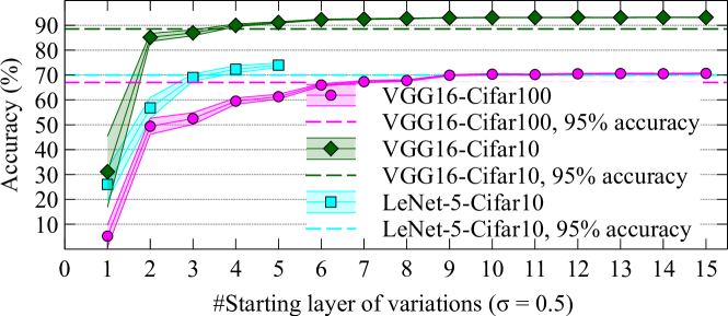
Figure 9: Lipschitz constant regularization against variations from a given layer to the last layer.

V Conclusion

In this paper, we have proposed the CorrectNet framework to recover inference accuracy of in-memory analog computing platforms under variations. The proposed framework consists of error suppression by training with Lipschitz constant regularization and error compensation for sensitive layers. With only a marginal overhead, the CorrectNet framework can recover inference accuracy from as low as 1.69% under variations and noise back to more than 95% of their original accuracy.

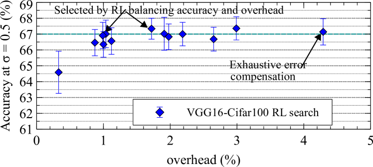
Figure 10: RL search for locations and parameters of error compensation.

References

- [1] A. Krizhevsky, I. Sutskever, and G. E. Hinton, “Imagenet classification with deep convolutional neural networks,” Advances in neural information processing systems, vol. 25, pp. 1097–1105, 2012.
- [2] C.-C. Chiu, T. N. Sainath, Y. Wu et al., “State-of-the-art speech recognition with sequence-to-sequence models,” in IEEE Int. Conf. Acoustics, Speech, and Signal Proc. (ICASSP), 2018.
- [3] Y. LeCun, Y. Bengio, and G. Hinton, “Deep learning,” Nature, vol. 521, pp. 436–444, 2015.
- [4] P. Chi, S. Li, C. Xu, T. Zhang, J. Zhao, Y. Liu, Y. Wang, and Y. Xie, “Prime: A novel processing-in-memory architecture for neural network computation in ReRAM-based main memory,” in International Symposium on Computer Architecture (ISCA), 2016.
- [5] A. Shafiee, A. Nag, N. Muralimanohar, R. Balasubramonian, J. P. Strachan, M. Hu, R. S. Williams, and V. Srikumar, “ISAAC: A convolutional neural network accelerator with in-situ analog arithmetic in crossbars,” in International Symposium on Computer Architecture (ISCA), 2016.
- [6] D. Niu, Y. Chen, C. Xu, and Y. Xie, “Impact of process variations on emerging memristor,” in ACM/IEEE Des. Autom. Conf. (DAC), 2010.
- [7] B. Liu, H. Li, Y. Chen, X. Li, Q. Wu, and T. Huang, “Vortex: Variation-aware training for memristor X-bar,” in ACM/IEEE Des. Autom. Conf. (DAC), 2015.
- [8] G. Charan, J. Hazra, K. Beckmann et al., “Accurate inference with inaccurate RRAM devices: Statistical data, model transfer, and on-line adaptation,” in ACM/IEEE Des. Autom. Conf. (DAC), 2020.
- [9] A. Mohanty, X. Du, P.-Y. Chen, J.-S. Seo, S. Yu, and Y. Cao, “Random sparse adaptation for accurate inference with inaccurate multi-level RRAM arrays,” in IEEE Int. Electron Dev. Meeting (IEDM), 2017.
- [10] Y. Zhu, G. L. Zhang, T. Wang, B. Li, Y. Shi, T.-Y. Ho, and U. Schlichtmann, “Statistical training for neuromorphic computing using memristor-based crossbars considering process variations and noise,” in IEEE Des., Autom., and Test Europe Conf. (DATE), 2020.
- [11] Y. Long, X. She, and S. Mukhopadhyay, “Design of reliable DNN accelerator with un-reliable ReRAM,” in IEEE Des., Autom., and Test Europe Conf. (DATE), 2019.
- [12] L. Chen, J. Li, Y. Chen, Q. Deng, J. Shen, X. Liang, and L. Jiang, “Accelerator-friendly neural-network training: Learning variations and defects in RRAM crossbar,” in IEEE Des., Autom., and Test Europe Conf. (DATE), 2017.
- [13] K. Simonyan and A. Zisserman, “Very deep convolutional networks for large-scale image recognition,” in Int. Conf. Learn. Repr. (ICLR), 2015.
- [14] Y. LeCun, B. Boser, J. S. Denker, D. Henderson, R. E. Howard, W. Hubbard, and L. D. Jackel, “Backpropagation applied to handwritten Zip code recognition,” Neural computation, vol. 1, no. 4, pp. 541–551, 1989.
- [15] H. Gouk, E. Frank, B. Pfahringer, and M. J. Cree, “Regularisation of neural networks by enforcing Lipschitz continuity,” Machine Learning, vol. 110, no. 2, pp. 393–416, 2021.
- [16] M. Cisse, P. Bojanowski, E. Grave, Y. Dauphin, and N. Usunier, “Parseval networks: Improving robustness to adversarial examples,” in Int. Conf. Machine Learn. (ICML), 2017.
- [17] J. Lin, C. Gan, and S. Han, “Defensive quantization: When efficiency meets robustness,” in Int. Conf. Learn. Repr. (ICLR), 2019.
- [18] A. Kosta, E. Soufleri, I. Chakraborty, A. Agrawal, A. Ankit, and K. Roy, “HyperX: A hybrid RRAM-SRAM partitioned system for error recovery in memristive xbars,” in IEEE Des., Autom., and Test Europe Conf. (DATE), 2022, pp. 88–91.
- [19] C. E. Shannon, “A mathematical theory of communication,” The Bell system technical journal, vol. 27, no. 3, pp. 379–423, 1948.