Entangled atomic ensemble and YIG sphere in coupled microwave cavities

Abstract

We present a scheme to generate distant bipartite and tripartite entanglement between an atomic ensemble and a yttrium iron garnet (YIG) sphere in coupled microwave cavities. The system we consider has five excitation modes namely cavity-1 photons, atomic ensemble, cavity-2 photons, magnon and phonon modes in YIG sphere. We show that significant bipartite entanglement exists between indirectly coupled subsystems in the cavities, which is robust against temperature. Moreover, we present suitable detuning parameters for a significant tripartite entanglement of ensemble, magnon, and phonon modes. We also demonstrate the existence of tripartite entanglement between magnon and phonon modes of YIG sphere with indirectly coupled cavity photons. Further, we show that cavity-cavity coupling strength affects both the degree and transfer of quantum entanglement between various subsystems. It follows that an appropriate cavity-cavity coupling optimizes the distant entanglement by increasing the entanglement strength and critical temperature for its existence.

I Introduction

Quantum entanglement is recognized as the most fascinating aspect of quantum formalism [1]. It has applications in quantum information processing, quantum networking, quantum dense coding, quantum-enhanced metrology, and so on [2, 3, 4, 5]. Therefore, its realization through physical resources used in information processing and communication protocols necessitates a scale above subatomic level for the ease of experimental implementation [6]. That is why there is a growing attention towards the exploration of quantum mechanical effects at macroscopic level. The advancement in micro and nanofabrication in recent years provided novel platforms to study macroscopic entanglement. Cavity optomechanics is one such system which received a lot of attention during the past decade [7, 8]. Among other applications [9, 10], cavity optomechanics enables quantum state transfer between different modes of electromagnetic fields [11, 12] which has central role in quantum information processing networks. Moreover, a possible platform for quantum information processing is offered by atomic ensembles. They can serve as valuable memory nodes for quantum communication networks due to their longer coherence duration and collective amplification effect for their nonlinear interaction with photons [13]. Another promising physical platform is yttrium iron garnet (YIG), a ferrimagnetic material, due to its high spin density and low decay rates of collective spin excitations (i.e., Kittel mode [14]) resulting in the strong coupling between Kittel mode and cavity photons [15, 16, 17, 18].

Since the initial experiments, many hybrid quantum systems based on quantum magnonics have been studied for their possible applications in quantum technologies [19, 20, 21, 22]. Magnon Cavity QED is a relatively newer field and a potential candidate for studying new features of strong-coupling QED. The observation of bi-stability and the single superconducting qubit coupling to the Kittel mode are interesting developments in this field [23, 24]. Li et al. illustrated how to create tripartite entanglement in a system of microwave cavity photons entangled to the magnon and phonon modes of a YIG sphere in a magnomechanical cavity [25]. It was followed by an investigation of magnon-magnon entanglement between two YIG spheres in cavity magnomechanics [26]. Later, Wu et al. investigated magnon-magnon entanglement between two YIG spheres in cavity optomagnonics [27]. Likewise, Ning and Yin theoretically demonstrated the entanglement of magnon and superconducting qubit utilizing a two-mode squeezed-vacuum microwave field in coupled cavities [28]. Yang et al. explored nonreciprocal transmission and entanglement in two-cavity magnomechanical system [29]. It was succeeded by the study of long-range generation of magnon-magnon entangled states via qubits [30].

Potential schemes for distant entanglement between disparate systems are increasingly considered for testing fundamental limits to quantum theory and possible applications in quantum networks [31]. In an interesting study, Joshi et al. theoretically examined whether two spatially distant cavities connected by an optical fiber may produce quantum entanglement between mechanical and optical modes [32]. Likewise, many researchers theoretically explored other schemes for transferring entanglement at a distance which includes an array of three optomechanical cavities for the study of the entanglement between different mechanical and optical modes [33] and a doubly resonant cavity with a gain medium of cascading three-level atoms placed in it to investigate entanglement transfer from two-mode fields to the two movable mirrors [34]. In double cavity optomechanical system, Liao et al. quantified entanglement of macroscopic mechanical resonators by the concurrence [35]. It was followed by a study of entanglement transfer from the inter cavity photon-photon entanglement to an intracavity photon-phonon via two macroscopic mechanical resonators. Afterwards, Bai et al. proposed a scheme of two-cavity coupled optomechanical system with atomic ensemble and a movable mirror in distinct cavities through which they showed ensemble-mirror entanglement and entanglement transfer between different subsytems [36].

In the past, several cavity optomechanical systems have been studied for entanglement with atomic medium [37, 36, 38, 39]. However, to the best of our knowledge, distant entanglement of atomic ensemble and YIG sphere in microwave cavities has not been reported yet. In this paper, we present a method for entangling atomic ensemble to mechanical and Kittel modes in YIG sphere placed within coupled microwave cavities. In our study, we have considered an atomic ensemble containing $N\sim 10^{7}$ [40, 41] atoms and YIG sphere with a typical diameter of $250\,{\mu}$m  [42], a promising platform to study distant macroscopic entanglement. We show that significant bipartite and tripartite entanglement exists between the magnon and phonon modes of YIG sphere placed in cavity-2 with the atomic ensemble and cavity-1 photons. It is interesting to find that YIG sphere can be entangled to indirectly coupled cavity field. We illustrate that this distant entanglement can be controlled by varying cavity-cavity coupling strength.

II system model and Hamiltonian

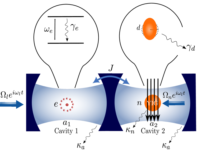
Figure 1: Schematic representation of two single-mode cavities coupled to each other with coupling strength $J$ incorporating an atomic ensemble of $N$ two-level atoms characterized by intrinsic frequency $\omega_{e}$ placed in cavity 1 and a YIG sphere placed in cavity 2. An external laser field drives cavity at frequency $\omega_{l}$ with strength $\Omega_{l}$. Correspondingly, a microwave magnetic field at frequencey $\omega_{l}$ with strength $\Omega_{n}$ drives the magnon modes of YIG sphere enhancing the magnomechanical coupling. YIG sphere is concurrently influenced by the cavity’s magnetic field, bias magnetic field and the drive magnetic field, all orthogonal to each other at the site of YIG sphere. The decay rate of cavity modes ($a_{1}$ and $a_{2}$), atomic ensemble ($e$), magnon mode ($n$) and phonon mode ($d$) associated with the YIG sphere are given by $\kappa_{a}$ ,$\gamma_{e}$, $\kappa_{n}$, and $\gamma_{d}$, respectively.

We consider a hybrid coupled-cavity magnomechanical system which consists of two single-mode cavities with resonance frequency $\omega_{k}$ $(k=1,2)$ encasing an atomic ensemble and a YIG sphere as shown in Fig. 1. Our coupled system has five excitation modes namely microwave electromagnetic modes in cavity 1 and cavity 2, magnon and phonon modes in YIG sphere, and atomic excitation in cavity 1.

In cavity 2, a YIG sphere is placed close to the maximum magnetic field of cavity mode and is simultaneously acted upon by a bias magnetic field, thus establishing the photon-magnon coupling. The external bias magnetic field excites the magnon modes. The magnetic field of the cavity mode interacts with Kittle mode via magnetic dipole interaction, in which spins evenly precess in the ferrimagnetic sphere. The bias field B and the gyromagnetic ratio $\Gamma$ control the magnon frequency, i.e., $\omega_{n}=\Gamma\textbf{B}$. Varying magnetization in the YIG sphere results in magnetostriction leading to the interplay of energy between magnon and phonon modes in it.

In cavity 1, an ensemble of $N$ two-level atoms with transition frequency $\omega_{e}$ interacts with the cavity field. The atoms constituting the ensemble are individually characterized by the spin-1/2 Pauli matrices $\sigma_{+},\sigma_{-}$, and $\sigma_{z}$. Collective spin operators of atomic polarization for the atomic ensemble are described as $S_{+,-,z}=\sum_{i=1}^{N}\sigma_{+,-,z}^{(i)}$, and they follow the commutation relations $\left[S_{+},S_{-}\right]=S_{z}$ and $\left[S_{z},S_{\pm}\right]=\pm 2S_{\pm}$ [36]. The operators $S_{\pm}$ and $S_{z}$ may be represented in terms of the bosonic annihilation and creation operators $e$ and $e^{\dagger}$ by using the Holstein-Primakoff transformation [43, 44, 45]: $S_{+}=e^{\dagger}\sqrt{N-e^{\dagger}e}\simeq\sqrt{N}e^{\dagger}$, $S_{-}=\sqrt{N-e^{\dagger}e}e\simeq\sqrt{N}e$, $S_{z}=e^{\dagger}e-N/2$, where $e$ and $e^{\dagger}$ follow commutation relation $\left[e,e^{\dagger}\right]=1$. This transformation is valid only when the population of atoms in the ground state is large compared to the atoms in the excited state so that $S_{z}\simeq\left\langle S_{z}\right\rangle\simeq-N$ [40].

To simplify our analysis, we have considered both the frequency of drive laser field and drive magnetic field to be $\omega_{l}$. The Hamiltonian describing the system under rotating-wave approximation in a frame rotating with the frequency of the drive fields ($\omega_{l}$) is given by:

$$H/\hbar= \sum_{k=1}^{2}\Delta_{k}a_{k}^{\dagger}a_{k}+\Delta_{e}e^{\dagger}e+\Delta_{n}n^{\dagger}n+\frac{\omega_{d}}{2}\left(x^{2}+y^{2}\right)$$

$$+g_{nd}n^{\dagger}nx+J\left(a_{1}^{\dagger}a_{2}+a_{1}a_{2}^{\dagger}\right)+G_{ae}\left(ea_{1}^{\dagger}+e^{\dagger}a_{1}\right)$$

$$+g_{na}\left(a_{2}n^{\dagger}+a_{2}^{\dagger}n\right)+i\Omega_{l}\left(a_{1}^{\dagger}-a_{1}\right)$$

$$+i\Omega_{n}\left(n^{\dagger}-n\right).$$ (1)

In Eq. (II), the energy associated with cavity (1 and 2), atomic excitation, and magnon modes is represented in the first four terms where $a_{k}\left(a_{k}^{\dagger}\right)$, $e\left(e^{\dagger}\right)$, and $n\left(n^{\dagger}\right)$ are the annihilation (creation) operators of cavity, collective atomic excitation, and magnon mode, respectively. Here, $\Delta_{k}$ ($k=1,2$), $\Delta_{e}$, and $\Delta_{n}$ are the detunings of cavity mode’s frequency $\omega_{k}$ ($k=1,2$), the intrinsic frequency of two-level atoms in the atomic ensemble $\omega_{e}$, and magnon mode’s frequency $\omega_{n}$ with respect to the drive field’s frequency $\omega_{l}$, i.e., $\Delta_{k}=\omega_{k}-\omega_{l}$ ($k=1,2$), $\Delta_{e}=\omega_{e}-\omega_{l}$, and $\Delta_{n}=\omega_{n}-\omega_{l}$. Rotating-wave approximation holds when $\omega_{k}(k=1,2),\omega_{n},\omega_{e}\gg$ $g_{na},\kappa_{a},\kappa_{n},\gamma_{e}$ (which is satisfied in cavity magnomechanics by experimentally feasible parameters) [46]. The fifth term in Eq. (II) is the energy of the mechanical mode (phonon mode) of frequency $\omega_{d}$ with dimensionless position $x$ and momentum $y$ operators satisfying $[x,y]=i$. The next four terms describe the interaction of all coupled subsystems in the cavity system encompassing coupling of magnon and phonon, cavity 1 and cavity 2, collective atomic excitation and cavity 1, cavity 2 and magnon modes with strength $g_{nd}$, $J$, $G_{ae}$, and $g_{na}$, respectively. The magnomechanical coupling strength $g_{nd}$, resulting from magnetostrictive interaction, is typically weak, but it is enhanced by the drive microwave field with frequency $\omega_{l}$ applied at the site of YIG. The coupling rate of collective atomic excitation with cavity mode $G_{ae}=g\sqrt{N}$ where $g$ is the atom-cavity coupling strength defined as $g=\nu\sqrt{\omega_{1}/2\hbar\epsilon_{0}V}$, with $\nu$ the dipole moment of atomic transition, $V$ the volume of the cavity, and $\epsilon_{0}$ the permittivity of free space. With reference to the eighth term, when the coherent energy exchange rate between light and matter is faster than their decay rates, the coupling strength between magnon and photon reaches the strong coupling regime, i.e., $g_{na}>\kappa_{a},\kappa_{n}$ [15, 14, 46, 17, 18]. The second-last term describes a microwave field driving cavity 1 with Rabi frequency, $\Omega_{l}=\sqrt{2{P\kappa_{a}}/\hbar\omega_{l}}$ which depends on the input power $P$ of the drive field and the decay rate $\kappa_{a}$ of the cavity. Similarly, we also consider a magnon-mode drive field (last term in Eq. (II)) with Rabi frequency $\Omega_{n}=\frac{\sqrt{5}}{4}\Gamma\sqrt{N_{s}}B_{0}$ with $\Gamma$ the gyromagnetic ratio, $N_{s}$ the total number of spins, and $B_{0}$ the applied field’s amplitude. In case of YIG sphere, $\Gamma/2\pi=28$ GHz/T, and $N_{s}=\rho V_{s}$ with volume $V_{s}$ and spin density $\rho=4.22\times 10^{27}\mathrm{~{}m}^{-3}$ of the sphere [25]. We assume low-lying excitations while deriving $\Omega_{n}$, i.e., $\left\langle n^{\dagger}n\right\rangle\ll 2N_{s}\varsigma$, where $\varsigma=\frac{5}{2}$ is the spin number of the ground state $\mathrm{Fe}^{3+}$ ion in YIG [25]. At a temperature $T$, the equilibrium mean thermal photon [$a_{k}$ ($k=1,2$)], magnon ($n$), and phonon ($d$) number is given by $Z_{h}(\omega_{h})=[\exp[(\hbar\omega_{h}/k_{B}T)]-1]^{-1}$ $(h=a_{k},n,d)$, where $k_{B}$ is the Boltzmann constant.

To investigate the dynamics of the coupled magnomechanical cavity system, we formulate a set of non-linear quantum Langevin equations (QLEs) by adding corresponding dissipation and fluctuation terms to the Heisenberg equations of motion given by:

$$\dot{a}_{1}=-\left(\kappa_{a}+i\Delta_{1}\right)a_{1}-iG_{ae}e-iJa_{2}+\sqrt{2\kappa_{a}}a_{1}^{in}+\Omega_{l},$$

$$\dot{a}_{2}=-\left(\kappa_{a}+i\Delta_{2}\right)a_{2}-iJa_{1}-ig_{na}n+\sqrt{2\kappa_{a}}a_{2}^{in},$$

$$\dot{e}=-\left(\gamma_{e}+i\Delta_{e}\right)e-iG_{ae}a_{1}+\sqrt{2\gamma_{e}}e^{in},$$

$$\dot{n}=-\left(i\Delta_{n}+\kappa_{n}\right)n-ig_{na}a_{2}-ig_{nd}nx+\Omega_{n}+\sqrt{2\kappa_{n}}n^{in},$$

$$\dot{x}=\omega_{d}y,\;\dot{y}=-\omega_{d}x-\gamma_{d}y-g_{nd}n^{\dagger}n+\xi$$ (2)

with zero-mean input noise operators $a_{k}^{in}$, $e^{in}$, $n^{in}$ and $\xi$ for $k^{th}$ cavity, atomic-excitation, magnon, and phonon modes, respectively. The parameters $\gamma_{e}$ and $\gamma_{d}$ are the atomic decay rate and the mechanical damping rate, respectively. The input noise operators under Markovian approximation, which is valid for large mechanical quality factor, $Q=\omega_{d}/\gamma_{d}\gg 1$ are characterized by the following non-vanishing correlation functions that are delta-correlated in time domain [47]: $\langle a_{1}^{\text{in }}(\tau)a_{1}^{in\dagger}(\tau^{\prime})\rangle=[Z_{a_{1}}(\omega_{a_{1}})+1]\delta(\tau-\tau^{\prime})$, $\langle a_{2}^{\text{in }}(\tau)a_{2}^{in\dagger}(\tau^{\prime}t)\rangle=[Z_{a_{2}}(\omega_{a_{2}})+1]\delta(\tau-\tau^{\prime})$, $\langle e^{in}(\tau)e^{in\dagger}(\tau^{\prime})\rangle=\delta(\tau-\tau^{\prime})$, $\langle n^{\text{in }}(\tau)n^{\text{in }\dagger}(\tau^{\prime})\rangle=[Z_{n}(\omega_{n}+1]\delta(\tau-\tau^{\prime})$, $\langle n^{\text{in }\dagger}(\tau)n^{in}(\tau^{\prime})\rangle=Z_{n}(\omega_{n})\delta(\tau-\tau^{\prime})$, and $\langle\xi(\tau)\xi(\tau^{\prime})+\xi(\tau^{\prime})\xi(\tau)\rangle/2\simeq\gamma_{d}[2Z_{d}(\omega_{d})+1]\delta(\tau-\tau^{\prime})$, where $\tau$ and $\tau^{\prime}$ denote two distinct times.

From the quantum Langevin Eq. (II), we obtain the expressions for the steady state values of cavities, ensemble, magnon, and phonon mode operators given by:

$$\left\langle a_{1}\right\rangle=\frac{\Omega_{l}\left(\kappa_{a}+i\Delta_{2}\right)\left(\kappa_{n}+i\tilde{\Delta}_{n}\right)\left(\gamma_{e}+i\Delta_{e}\right)+g_{na}^{2}\Omega_{l}\left(\gamma_{e}+i\Delta_{e}\right)-g_{na}\Omega_{n}J\left(\gamma_{e}+i\Delta_{e}\right)}{S},$$ (3)

$$\left\langle a_{2}\right\rangle=\frac{-iJ\left(\kappa_{n}+i\tilde{\Delta}_{n}\right)\left\langle a_{1}\right\rangle-ig_{na}\Omega_{n}}{\left(\kappa_{a}+i\Delta_{2}\right)\left(\kappa_{n}+i\tilde{\Delta}_{n}\right)+g_{na}^{2}},\,\,\langle e\rangle=\frac{-iG_{ae}\left\langle a_{1}\right\rangle}{\left(\gamma_{e}+i\Delta_{e}\right)},\,\,\langle n\rangle=\frac{\Omega_{n}-ig_{na}\left\langle a_{2}\right\rangle}{i\tilde{\Delta}_{n}+\kappa_{n}},$$

$$\langle x\rangle=-\left(\frac{g_{nd}}{\omega_{d}}\right)|\langle n\rangle|^{2},\,\,\langle y\rangle=0,$$

where
$S=(\kappa_{a}+i\Delta_{1})(\gamma_{e}+$ $i\Delta_{e})[(\kappa_{a}+i\Delta_{2})(\kappa_{n}+$ $i\tilde{\Delta}_{n})+$ $g_{na}^{2}]$ $-G_{ae}^{2}[(\kappa_{a}+i\Delta_{2})$ $(\kappa_{n}+i\tilde{\Delta}_{n})$ $+g_{na}^{2}]$ $+J^{2}(\gamma_{e}+i\Delta_{e})(\kappa_{n}$ $+i\tilde{\Delta}_{n})$,
and the effective magnon detuning $\tilde{\Delta}_{n}=\Delta_{n}+g_{nd}\langle x\rangle$. To analyze the steady-state entanglement of the system, we linearize the dynamics of coupled cavity system. We assume that the cavity is intensely driven with a very high input power, resulting in significant steady state amplitudes for the intracavity fields and magnon modes, respectively, i.e., $\left|\langle a_{k}\rangle\right|\gg 1$ ($k=1,2$) [48] and $|\langle n\rangle|\gg 1$ [25]. For a proper choice of drive field’s reference phase, $\langle a_{k}\rangle$ may be treated real [48]. Moreover, the bosonic description of atomic polarization may only be used when the single-atom excitation probability is noticeably below 1. The conditions of large amplitudes of intracavity fields at steady state and low excitation limit of atoms in the ensemble are simultaneously satisfied only when $g^{2}/\left(\Delta_{e}^{2}+\gamma_{e}^{2}\right)\ll\left|\langle a_{1}\rangle\right|^{-2}\ll 1$. This necessitates a weak atom-cavity coupling [40]. Hence, in the strong driving limit, we can neglect the second order fluctuation terms, so the operator $P$ ($P=a_{k},e,n,x,y$) can be written as $P=\langle P\rangle+\delta P$ where $\langle P\rangle$ represents the steady state part while $\delta P$ represents the zero-mean fluctuation associated with $P$. Further, we define quadrature fluctuations ($\delta U_{1}(t)$, $\delta W_{1}(t)$, $\delta U_{2}(t)$, $\delta W_{2}(t)$, $\delta u_{1}(t)$, $\delta w_{1}(t)$, $\delta x(t)$, $\delta y(t)$, $\delta u_{2}(t)$, $\delta w_{2}(t)$), with $\delta U_{1}=\left(\delta a_{1}+\delta a_{1}^{\dagger}\right)/\sqrt{2}$, $\delta W_{1}=i\left(\delta a_{1}^{\dagger}-\delta a_{1}\right)/\sqrt{2}$, $\delta U_{2}=(\delta a_{2}+\delta a_{2}^{\dagger})/\sqrt{2}$, $\delta W_{2}=i(\delta a_{2}^{\dagger}-\delta a_{2})/\sqrt{2}$, $\delta u_{1}=(\delta n+\delta n^{\dagger})/\sqrt{2}$, $\delta w_{1}=i(\delta n^{\dagger}-\delta n)/\sqrt{2}$, $\delta u_{2}=(\delta e+\delta e^{\dagger})/\sqrt{2}\,$ and $\delta w_{2}=i(\delta e^{\dagger}-\delta e)/\sqrt{2}$, to work out a set of linearized quantum Langevin equations

$$\dot{r}(t)=Ar(t)+o(t);$$ (4)

$r(t)$ represents the fluctuation operator in the form of quadrature fluctuations: $r(t)^{T}=[\delta U_{1}(t),\delta W_{1}(t),\delta U_{2}(t),$ $\delta W_{2}(t),\delta u_{1}(t),$ $\delta w_{1}(t),\delta x(t),$ $\delta y(t),\delta u_{2}(t),$ $\delta w_{2}(t)]$, $o(t)$ denotes the noise operators represented as: $o(t)^{T}=[\sqrt{2\kappa_{a}}$ $U_{1}^{in}(t),$ $\sqrt{2\kappa_{a}}$ $W_{1}^{in}(t),$ $\sqrt{2\kappa_{a}}U_{2}^{in}(t),$ $\sqrt{2\kappa_{a}}W_{2}^{in}(t),$ $\sqrt{2\kappa_{n}}u_{1}^{in}(t),$ $\sqrt{2\kappa_{n}}w_{1}^{in}(t),$ $0$, $\xi(t),\,\sqrt{2\gamma_{e}}u_{2}^{in}(t),$ $\sqrt{2\gamma_{e}}w_{2}^{in}(t)]$, and $A$ is the drift matrix:

$$A=\begin{pmatrix}-\kappa_{a}&\Delta_{1}&0&J&0&0&0&0&0&G_{ae}\\ -\Delta_{1}&-\kappa_{a}&-J&0&0&0&0&0&-G_{ae}&0\\ 0&J&-\kappa_{a}&\Delta_{2}&0&g_{na}&0&0&0&0\\ -J&0&-\Delta_{2}&-\kappa_{a}&-g_{na}&0&0&0&0&0\\ 0&0&0&g_{na}&-\kappa_{n}&\tilde{\Delta}_{n}&-G_{nd}&0&0&0\\ 0&0&-g_{na}&0&-\tilde{\Delta}_{n}&-\kappa_{n}&0&0&0&0\\ 0&0&0&0&0&0&0&\omega_{d}&0&0\\ 0&0&0&0&0&G_{nd}&-\omega_{d}&-\gamma_{d}&0&0\\ 0&G_{ae}&0&0&0&0&0&0&-\gamma_{e}&\Delta_{e}\\ -G_{ae}&0&0&0&0&0&0&0&-\Delta_{e}&-\gamma_{e}\end{pmatrix}.$$ (5)

The linearized quantum Langevin equations [see Eq. (4)] correspond to an effective linearized Hamiltonian, which ensures the Gaussian state of the system when it is stable. Thus, the linearized dynamics of the system along with the Gaussian nature of the noises leads to the continuous-variable five-mode Gaussian state of the steady states corresponding to its quantum fluctuations. Routh-Hurwitz criterion is used to work out the stability conditions for our linearized system [49]. The system becomes stable and attain its steady state only when real parts of all eigenvalues of the drift matrix ($A$) are negative. The steady state Covariance Matrix (CM), which describes the variance within each subsystem and the covariance across several subsystems, is generated from the following Lyapunov equation when the stability requirements are met [50]:

$$A\mathcal{V}+\mathcal{V}A^{T}=-D,$$ (6)

where $D=\operatorname{diag}\,[\kappa_{a}(2\,Z_{a}+1),\kappa_{a}(2\,Z_{a}+1),\kappa_{a}(2\,Z_{a}+1),$ $\kappa_{a}(2\,Z_{a}+1)$, $\kappa_{n}\left(2Z_{n}+1\right)$, $\kappa_{n}\left(2Z_{n}+1\right)$, $0$, $\gamma_{d}(2\,Z_{d}+1),\gamma_{e},\gamma_{e}]^{T}$ is the diffusion matrix, for the corresponding decays originating from the noise correlations. To quantify bipartite entanglement among different subsystems of the coupled two-cavity system, we use logarithmic negativity ($\mathit{E_{N}}$) [51, 52]. We have five mode Gaussian state characterized by covariance matrix $\mathcal{V}$ which can be expressed in the form of block matrix:

$$\mathcal{V}=\left(\begin{array}[]{ccccc}\mathcal{V}_{a_{1}}&\mathcal{V}_{a_{1}a_{2}}&\mathcal{V}_{a_{1}n}&\mathcal{V}_{a_{1}d}&\mathcal{V}_{a_{1}e}\\ \mathcal{V}^{T}_{a_{1}a_{2}}&\mathcal{V}_{a_{2}}&\mathcal{V}_{a_{2}n}&\mathcal{V}_{a_{2}d}&\mathcal{V}_{a_{2}e}\\ {\mathcal{V}}^{T}_{a_{1}n}&\mathcal{V}^{T}_{a_{2}n}&\mathcal{V}_{n}&\mathcal{V}_{nd}&\mathcal{V}_{ne}\\ \mathcal{V}^{T}_{a_{1}d}&\mathcal{V}^{T}_{a_{2}d}&\mathcal{V}^{T}_{nd}&\mathcal{V}_{d}&\mathcal{V}_{de}\\ \mathcal{V}^{T}_{a_{1}e}&\mathcal{V}^{T}_{a_{2}e}&\mathcal{V}^{T}_{ne}&\mathcal{V}^{T}_{de}&\mathcal{V}_{e}\\ \end{array}\right),$$ (7)

where each block is a $2\times 2$ matrix. Here, diagonal blocks represent the variance within each subsystem [(cavity 1) photon, (cavity 2) photon, magnon, phonon, and ensemble]. The correlations between any two distinct degrees of freedom of the entire magnomechanical system are represented by the off-diagonal blocks, which are covariances across distinct subsystems [36]. Following the Simon’s criterion [53] to judge non-separability of the transposed modes in the transposed submatrix derived from the covariance matrix $\mathcal{V}$, we compute logarithmic negativity numerically. The covariance matrix ($10\times 10$) $\mathcal{V}$ is reduced to a submatrix $\mathcal{V}_{l}$ ($4\times 4$) in order to evaluate the covariance between the subsystems. For instance, the submatrix representing the covariance of cavity 1 and cavity 2 subystem is determined by the first four rows and columns of $\mathcal{V}$. We can represent $\mathcal{V}_{l}$ of cavity 1-cavity 2 subsystems in the following way [36]:

$$\mathcal{V}_{l}=\left(\begin{array}[]{cc}\mathcal{V}_{a_{1}}&\mathcal{V}_{a_{1}a_{2}}\\ \mathcal{V}_{a_{1}a_{2}}^{T}&\mathcal{V}_{a_{2}}\end{array}\right),$$ (8)

where $a_{1}$ index the cavity 1 subsystem and $a_{2}$ index the cavity 2 subsystem. Similarly, the covariance of other subsystems can be determined by considering their corresponding rows and columns in $\mathcal{V}$. Then, transposed covariance sub-matrix $\tilde{\mathcal{V}_{l}}$ is obtained by partial transposition of $\mathcal{V}_{l}$ employing $\tilde{\mathcal{V}}_{l}=\mathcal{T}_{1\mid 2}\mathcal{V}_{l}\mathcal{T}_{1\mid 2}$, where $\mathcal{T}_{1\mid 2}=\operatorname{diag}(1,-1,1,1)$ realizes partial transposition at the level of covariance matrices [53]. Then, we compute the the minimum symplectic eigenvalue $\tilde{f}_{-}$ of the transposed CM $\tilde{\mathcal{V}}_{l}$ using $\tilde{f}_{-}=\min\operatorname{eig}\left|i\Theta_{2}\tilde{\mathcal{V}}_{l}\right|$ with $\Theta_{2}=\oplus_{j=1}^{2}i\sigma_{y}$ and $\sigma_{y}$ the $y$-Pauli matrix [25]. If the smallest eigenvalue is less than 1/2, the inseparability of the transposed modes is ensured, i.e., the modes are entangled. $\mathit{E_{N}}$ is evaluated as [52]:

$$E_{N}\equiv\max\left[0,-\ln 2\tilde{f}_{-}\right].$$ (9)

Similarly, residual contangle $\mathcal{R}_{\tau}^{min}$ [54], which is a continuous variable analogue of tangle for discrete variable tripartite entanglement [55], is used for the quantification of tripartite entanglement, which is defined as [54]:

$$\mathcal{R}_{\tau}^{\min}\equiv\min\left[\mathcal{R}_{\tau}^{o\mid nd},\mathcal{R}_{\tau}^{n\mid od},\mathcal{R}_{\tau}^{d\mid on}\right],$$ (10)

where $n$ stands for magnon whereas $d$ stands for phonon mode, $o=a_{1}$ for cavity-magnon-phonon tripartite entanglement, and $o=e$ for magnon-phonon-ensemble tripartite entanglement. In Eq. (10) $\mathcal{R}_{\tau}^{k\mid lm}$ is evaluated using $\mathcal{R}_{\tau}^{k\mid lm}\equiv C_{k\mid lm}-C_{k\mid l}-C_{k\mid m}\,(k,l,m=o,n,d)$, $C_{k\mid lm}$ is the squared one-mode-vs-two-modes logarithmic negativity $\mathit{E}_{k\mid lm}$ and $C_{k\mid l}$ is the contangle of subsystems of $k$ and $l$ [25], defined as the squared logarithmic negativity $\mathit{E}_{k\mid l}$ [52]. To compute $\mathit{E}_{k\mid lm}$ following the definition of logarithmic negativity given in Eq.(9), $\Theta_{2}=\oplus_{j=1}^{2}i\sigma_{y}$ is replaced by $\Theta_{3}=\oplus_{j=1}^{3}i\sigma_{y}$ and the transposed covariance matrix $\tilde{\mathcal{V}}$ is obtained by carrying out the partial transposition of covariance matrix $\mathcal{V}$, i.e., $\tilde{\mathcal{V}}=\mathcal{T}_{k\mid lm}\mathcal{V}\mathcal{T}_{k\mid lm}$, where the partial transposition matrices  [25] are: $\mathcal{T}_{1\mid 23}=\operatorname{diag}(1,-1,1,1,1,1)$, $\mathcal{T}_{2\mid 13}=\operatorname{diag}(1,1,1,-1,1,1)$, and $\mathcal{T}_{3\mid 12}=\operatorname{diag}(1,1,1,1,1,-1)$.

III Results and Discussion

In this section, we present the results of our numerical simulations. We have adopted the following experimentally feasible parameters for the system involving microwave cavities and YIG sphere in our simulations [25]: $\omega_{k}/{2\pi}=\omega_{n}/{2\pi}=10\,$GHz $(k=1,2)$, $\omega_{d}/{2\pi}=10\,$MHz, $\gamma_{d}/{2\pi}=10^{2}\,$Hz, $\kappa_{a}/{2\pi}=\kappa_{n}/{2\pi}=1\,$MHz, $g_{na}/{2\pi}=3.2\,$MHz, $G_{nd}/{2\pi}=4.8\,$MHz, and temperature $T=10\,$mK. Correspondingly, the atom-cavity coupling and atomic decay rate are considered of the order of megahertz, i.e, $G_{ae}/{2\pi}=6\,$MHz and $\gamma_{e}/{2\pi}=1\,$MHz. Further, the hopping rate $J$ between the cavities is also of the order of megahertz.

Bipartite Subsystems	Symbol for Entanglement
cavity 1-cavity 2	$E_{N}^{a_{1}a_{2}}$
cavity 1-ensemble	$E_{N}^{a_{1}e}$
cavity 1-magnon	$E_{N}^{a_{1}n}$
cavity 1-phonon	$E_{N}^{a_{1}d}$
cavity 2-ensemble	$E_{N}^{a_{2}e}$
cavity 2-magnon	$E_{N}^{a_{2}n}$
cavity 2-phonon	$E_{N}^{a_{2}d}$
magnon-ensemble	$E_{N}^{ne}$
phonon-ensemble	$E_{N}^{de}$

Table 1: Notation adopted for the representation of bipartite entanglement.

First, we discuss the results of bipartite entanglement. We have five different modes in coupled-cavity system, therefore entanglement can exist in any combination of two modes. However, the most significant entanglement is the entanglement of spatially distant subsystems, i.e., the entanglement of atomic ensemble and cavity 1 photons with phonon and magnon modes of YIG sphere placed in cavity 2. Interestingly, we observe promising results of macroscopic distant entanglement. We also illustrate entanglement transfer from phonon-ensemble ($de$) and magnon-ensemble ($ne$) subsystems to cavity 1 photons-phonon ($a_{1}d$) and cavity 1 photon-magnon subsystems ($a_{1}n$) when detuning parameters and cavity-cavity coupling strength are changed. In Table 1, we have summarized the symbols that we have adopted in our simulations to represent bipartite entanglement of different combinations of subsystems.

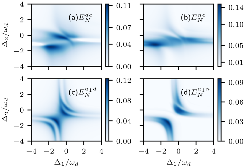
Figure 2: Density plot of bipartite (a) $E_{N}^{de}$, (b) $E_{N}^{ne}$, (c) $E_{N}^{a_{1}d}$, and (d) $E_{N}^{a_{1}n}$ versus normalized cavity 1 detuning $\Delta_{1}/{\omega_{d}}$ and cavity 2 detuning $\Delta_{2}/{\omega_{d}}$. In (a)-(b) $\Delta_{e}=-\omega_{d}$ whereas in (c)-(d) $\Delta_{e}=\omega_{d}$. In all cases, $\tilde{\Delta}_{n}=0.9\,\omega_{d}$ and $J=0.8\,\omega_{d}$.

In Fig. 2, we present four different distant bipartite entanglements as a function of dimensionless detuning of cavity 1 $\left(\Delta_{1}/\omega_{d}\right)$ and cavity 2 $\left(\Delta_{2}/\omega_{d}\right)$. We have considered magnon detuning $\tilde{\Delta}_{n}$ to be $0.9\,\omega_{d}$ (near resonant with blue sideband) while coupling between two cavities is $J=0.8\,\omega_{d}$. Fig. 2(a)-(b) illustrates ensemble-phonon ($E_{N}^{de}$) and ensemble-magnon ($E_{N}^{ne}$) entanglement for ensemble detuning $\Delta_{e}$ to be $-\omega_{d}$ (resonant with red sideband). Although ensemble and YIG sphere are placed in separate cavities, we find strong entanglement for both $E_{N}^{de}$ and $E_{N}^{ne}$. $E_{N}^{de}$ attains maximum value around $\Delta_{2}\approx-2\,\omega_{d}$ and $\Delta_{2}\approx 0$ corresponding to $\Delta_{1}\approx-2\,\omega_{d}$ and $\Delta_{1}\approx 0$. It can be seen that $E_{N}^{ne}$ is manifested primarily around $\Delta_{2}\,\approx-\omega_{d}$ in the entire range of $\Delta_{1}/\omega_{d}$. However, maximum $E_{N}^{ne}$ exists around $\Delta_{1}\approx-2.5\,\omega_{d}$. Similarly, we present cavity-1 photon-phonon ($E_{N}^{a_{1}d}$) and cavity-1 photon-magnon ($E_{N}^{a_{1}n}$) entanglement in Fig. 2(c)-(d) for $\Delta_{e}=-\omega_{d}$. Both systems exhibit strong entanglement around $\Delta_{1}\approx-\omega_{d}$ and $\Delta_{1}\approx 0$. If we follow $\Delta_{1}=\Delta_{2}$ line on the plane formed by $\Delta_{1}$ and $\Delta_{2}$, we observe that there are two distinct detuning regions for maximal $E_{N}$ on the density plots showing $E_{N}^{a_{1}d}$ and $E_{N}^{a_{1}n}$ compared to a single joint region along the $\Delta_{1}=-\Delta_{2}$ line.

For further analysis, we consider two cases. In the first case, cavity 1 and cavity 2 have the same detuning frequency with respect to the drive fields’ frequency, i.e., $\Delta_{1}=\Delta_{2}=\Delta_{a}$, (symmetric detuning). If the first cavity is red-detuned or blue-detuned, the second cavity is also red-detuned or blue-detuned, correspondingly. In the second case, cavity 1 and cavity 2 have opposite detuning frequency with respect to the drive fields’ frequency, i.e., $\Delta_{1}=-\Delta_{2}=-\Delta_{a}$, (non-symmetric detuning). If the first cavity is red-detuned, the second is blue-detuned and vice versa.

Figure 3: Density plot of $E_{N}^{de}$ versus normalized cavity detuning $\Delta_{a}/{\omega_{d}}$ and (a)-(b) magnon detuning $\tilde{\Delta}_{n}/{\omega_{d}}$ at $\Delta_{e}=-\omega_{d}$, and (c)-(d) ensemble detuning $\Delta_{e}/{\omega_{d}}$ at $\tilde{\Delta}_{n}=0.9\,\omega_{d}$. In (a) and (c) $\Delta_{a}/{\omega_{d}}=\Delta_{1}/{\omega_{d}}=\Delta_{2}/{\omega_{d}}$. However, $\Delta_{a}/{\omega_{d}}=-\Delta_{1}/{\omega_{d}}=\Delta_{2}/{\omega_{d}}$ in (c) and (d). The cavity-cavity coupling strength is taken to be $J=\omega_{d}$.

Next, we present phonon-ensemble entanglement ($E_{N}^{de}$) as a function of normalized cavity detuning $(\Delta_{a}/{\omega_{d}})$ against dimensionless magnon detuning $\tilde{\Delta}_{n}/{\omega_{d}}$ in Fig. 3(a)-(b) and ensemble detuning $\Delta_{e}/{\omega_{d}}$ in Fig. 3(c)-(d). For given parameters, effective magnon detuning $\tilde{\Delta}_{n}$ includes magnon detuning with respect to the drive field and frequency shift of almost $3$ MHz due to magnomechanical interaction. In the left panel, we have symmetric cavity field detuning while in the right panel, the detuning is non-symmetric. It can be seen in Fig. 3 (a)-(b) that significant entanglement is present for the complete range of effective magnon detuning. We note that the system remains stable for $\tilde{\Delta}_{n}$ from $0.4\,\omega_{d}$ to $2\,\omega_{d}$, however, we consider $0.6\leq\tilde{\Delta}_{n}/\omega_{d}\leq 1.4$, where we get stronger entanglement. While $E_{N}^{de}$ is significant for the chosen range of $\tilde{\Delta}_{n}$, it strongly depends on the choice of cavity field detuning. There are two distinct regions of cavity detuning where we find maximum entanglement. One region is around cavity resonance for both the symmetric and non-symmetric choices of detuning, while the other region depends on the choice. For the symmetric case, strong entanglement is also present around $\Delta_{a}\approx-1.75\,\omega_{d}$. However, for the non-symmetric case, this second region is around $\Delta_{a}\approx-\omega_{d}$. The lower panel in Fig. 3 shows that $E_{N}^{de}$ is maximum around $\Delta_{e}\approx-\omega_{d}$, while the choices of cavity detuning are approximately the same as discussed above in the previous case.

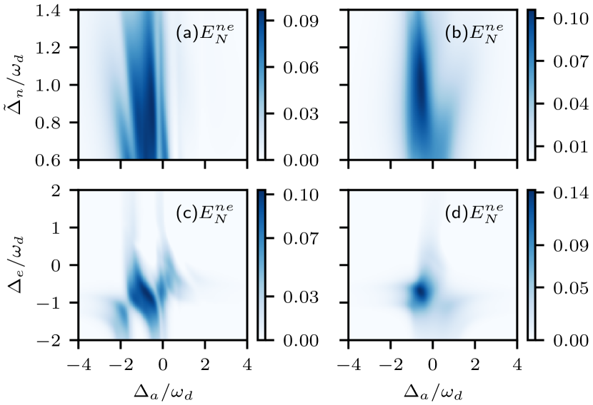
Figure 4: Density plot of $E_{N}^{ne}$ versus normalized cavity detuning $\Delta_{a}/\omega_{d}$ and (a)-(b) magnon detuning $\tilde{\Delta}_{n}/{\omega_{d}}$ at $\Delta_{e}=-\omega_{d}$, and (c)-(d) ensemble detuning $\Delta_{e}/{\omega_{d}}$ at $\tilde{\Delta}_{n}=0.9\,\omega_{d}$. In (a) and (c) $\Delta_{a}/{\omega_{d}}=\Delta_{1}/{\omega_{d}}=\Delta_{2}/{\omega_{d}}$. However, $\Delta_{a}/{\omega_{d}}=-\Delta_{1}/{\omega_{d}}=\Delta_{2}/{\omega_{d}}$ in (b) and (d). The cavity-cavity coupling strength is taken to be $J=0.8\,\omega_{d}$.

Fig. 4 shows magnon-ensemble entanglement ($E_{N}^{ne}$) as a function of normalized cavity detuning against dimensionless magnon detuning (upper panel) and ensemble detuning (lower panel). $E_{N}^{ne}$ is optimal around $\Delta_{a}\approx 0.5\,\omega_{d}$. Fig. 4(a)-(b) shows that $E_{N}^{ne}$ is significant for the whole range of $\tilde{\Delta}_{n}$ while it is maximum around $\Delta_{e}\approx-\omega_{d}$ as shown in Fig. 4(c)-(d). In both cases, we note that entanglement exists for a wider parameter space in symmetric detuning as compared to the non-symmetric detuning choice. Similar to $E_{N}^{de}$, $E_{N}^{ne}$ is also significant around $\Delta_{e}\approx-\omega_{d}$ and $\tilde{\Delta}_{n}\approx 0.9\,\omega_{d}$. As a consequence, we can say that bipartite entanglement of modes involving atomic ensemble and YIG sphere is most remarkable when magnon is resonant with stokes band while ensemble is resonant with anti-stokes band.

Fig. 5 shows $E_{N}^{a_{1}d}$ and $E_{N}^{a_{1}n}$ as a function of normalized cavity detuning and ensemble detuning. For the first case [see Fig. 5(a)-(c)], $E_{N}^{a_{1}d}$ and $E_{N}^{a_{1}n}$ exists both around $\Delta_{a}\approx-2\,\omega_{d}$ and $\Delta_{a}\approx 0$. For the second case [see Fig. 5(b)-(d)], $E_{N}^{a_{1}d}$ and $E_{N}^{a_{1}n}$ are observable only near resonance frequency of both cavities. In contrast to $E_{N}^{de}$ and $E_{N}^{ne}$, $E_{N}^{a_{1}d}$ and $E_{N}^{a_{1}n}$ are prominent when atomic ensemble is resonant with the anti-strokes band, i.e, at $\Delta_{e}\approx\omega_{d}$ and almost negligible at $\Delta_{e}=-\omega_{d}$ as depicted in Fig. 5.

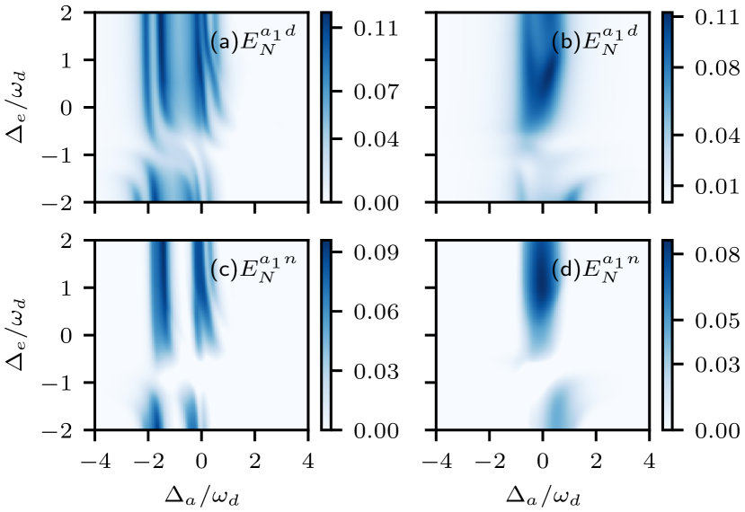
Figure 5: Density plot of $E_{N}^{a_{1}d}$ and $E_{N}^{a_{1}n}$ versus normalized cavity detuning $\Delta_{a}/\omega_{d}$ and ensemble detuning $\Delta_{e}/{\omega_{d}}$ at $J=0.8\,\omega_{d}$ and $\tilde{\Delta}_{n}=0.9\,\omega_{d}$. In (a) and (c) $\Delta_{a}/{\omega_{d}}=\Delta_{1}/{\omega_{d}}=\Delta_{2}/{\omega_{d}}$. However, $\Delta_{a}/{\omega_{d}}=-\Delta_{1}/{\omega_{d}}=\Delta_{2}/{\omega_{d}}$ in (b) and (d).

Fig. 6 illustrates the dependence of cavity-1 photon-phonon entanglement ($E_{N}^{a_{1}d}$) and cavity-1 photon-magnon entanglement ($E_{N}^{a_{1}n}$) on cavity-cavity coupling strength $J$ and cavity detuning $\Delta_{a}$. We chose $\tilde{\Delta}_{n}=0.9\,\omega_{d}$ and $\Delta_{e}=\omega_{d}$. As expected, the bipartite entanglement of these subsystems is non-existent in the absence of cavity-cavity coupling. For the symmetric cavity detuning [see Fig. 6(a)-(c)], entanglement first increases with increasing $J$ around $\Delta_{a}\approx 0.5\,\omega_{d}$, but beyond a certain value of $J$ further increase shifts the detuning region for optimal entanglement to the right and left of $\Delta_{a}\approx 0.5\,\omega_{d}$. However, for the non-symmetric detuning [see Fig. 6(b)-(d)] the trend is quite different. $E_{N}^{a_{1}d}$ and $E_{N}^{a_{1}n}$ increases with increasing coupling strength till a particular value of $J$. We note that the dependence on $J$ varies when a different value of $\Delta_{e}$ and $\tilde{\Delta}_{n}$ is considered. For the given parameters, $E_{N}^{a_{1}d}$ first increases as a function of J and then decreases, reaching a minimum at $J\approx 0.8\,\omega_{d}$ followed by an increasing trend up to $J\approx 1.5\,\omega_{d}$ and decreases afterwards, whereas $E_{N}^{a_{1}n}$ increases up to $J\approx\omega_{d}$ and gradually dies out thereafter. It is important to note that when $E_{N}^{a_{1}d}$ reaches the minimum around $J=0.8\,\omega_{d}$, $E_{N}^{a_{1}n}$ has maximum value. The reason lies in the entanglement transfer between different subsystems, which is further elaborated in the following analysis.

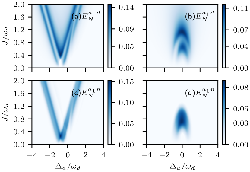
Figure 6: Density plot of $E_{N}^{a_{1}d}$ and $E_{N}^{a_{1}n}$ versus normalized cavity detuning $\Delta_{a}/\omega_{d}$ and coupling strength $J/\omega_{d}$ at $\tilde{\Delta}_{n}=0.9\,\omega_{d}$ and $\Delta_{e}=\omega_{d}$. In (a) and (c) $\Delta_{a}/{\omega_{d}}=\Delta_{1}/{\omega_{d}}=\Delta_{2}/{\omega_{d}}$. However, $\Delta_{a}/{\omega_{d}}=-\Delta_{1}/{\omega_{d}}=\Delta_{2}/{\omega_{d}}$ in (b) and (d).

Henceforth, we set $-\Delta_{1}=\Delta_{2}=\Delta_{a}$ in our simulations. The role of $J$ in the degree and dynamics of entanglement transfer between different subsystem is further elaborated in Fig. 7. At smaller $J$, there is a significant transfer of entanglement from $E_{N}^{nd}$ to $E_{N}^{a_{2}d}$ and $E_{N}^{a_{2}n}$ around $\Delta_{2}=-\omega_{d}$. This transfer not only decreases with increasing $J$, but there is also a corresponding decrease in the strength of $E_{N}^{a_{2}d}$ and $E_{N}^{a_{2}n}$. This decrease accounts for the corresponding increase in $E_{N}^{de}$ and $E_{N}^{ne}$. Another interesting feature is that at smaller $J$, maximum entanglement of $E_{N}^{a_{2}d}$, $E_{N}^{a_{2}n}$, $E_{N}^{de}$, and $E_{N}^{ne}$ subsystems lie in the detuning region when cavity 1 is resonant with the blue sideband while cavity 2 is resonant with the red sideband. However, the peaks of $E_{N}$ curves representing their entanglement gradually shifts from $\Delta_{a}\approx-\omega_{d}$ to $\Delta_{a}\approx 0$ as we move from $J=0.4\,\omega_{d}$ to $J=1.4\,\omega_{d}$ and the region for the existence of entanglement also broadens. Since we have considered $\Delta_{e}=-\omega_{d}$ in Fig. 7, $E_{N}^{a_{1}d}$ and $E_{N}^{a_{1}n}$ entanglement is quite weak in this parametric domain. Nonetheless, it is apparent that $E_{N}^{a_{1}d}$ and $E_{N}^{a_{1}n}$ entanglement also increases with increasing $J$.

Subsytems	$\mathbf{\Delta_{1}}$	$\mathbf{\Delta_{2}}$	$\mathbf{\tilde{\Delta}_{n}}$	$\mathbf{\Delta_{e}}$	$\mathbf{J}$
$E_{N}^{a_{1}n}$	$-1.41\,\omega_{d}$	$-0.68\,\omega_{d}$	$-0.65\,\omega_{d}$	$-1.63\,\omega_{d}$	$0.35\,\omega_{d}$
$E_{N}^{a_{1}d}$	$-0.04\,\omega_{d}$	$0.85\,\omega_{d}$	$0.77\,\omega_{d}$	$0.99\,\omega_{d}$	$1.28\,\omega_{d}$
$E_{N}^{ne}$	$0.76\,\omega_{d}$	$-0.52\,\omega_{d}$	$0.77\,\omega_{d}$	$-0.63\,\omega_{d}$	$0.8\,\omega_{d}$
$E_{N}^{de}$	$0.28\,\omega_{d}$	$-0.84\,\omega_{d}$	$0.6\,\omega_{d}$	$-1.07\,\omega_{d}$	$1.06\,\omega_{d}$

Table 2: Optimized parameters for $E_{N}^{a_{1}n}$, $E_{N}^{a_{1}d}$, $E_{N}^{ne}$, and $E_{N}^{de}$ used in Fig. 8.

Next, we present the results of our numerical simulations demonstrating the critical temperature ($T_{c}$) for $E_{N}^{de}$, $E_{N}^{ne}$, $E_{N}^{a_{1}d}$, and $E_{N}^{a_{1}n}$ in Fig. 8. Entangled subsystems magnon-ensemble and phonon-ensemble exhibit the most robust entanglement against temperature, which can last up to $200\mathrm{~{}mK}$. On the other hand, cavity 1 photon-magnon entanglement can survive temperatures up to $170\mathrm{~{}mK}$. However, cavity 1 photon-phonon subsystem can sustain their entanglement at as high temperature as $180\mathrm{~{}mK}$. Each curve in Fig. 8 is plotted for an optimized set of parameter values given in Table 2.

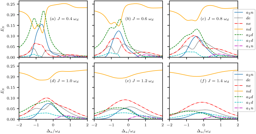
Figure 7: Line plot illustrating the effect of cavity-cavity coupling rate $J$ against cavity detuning $\Delta_{a}/{\omega_{d}}=-\Delta_{1}/{\omega_{d}}=\Delta_{2}/{\omega_{d}}$ on bipartite entanglement of cavity 2 photon-magnon ($a_{2}n$), phonon-ensemble ($de$), magnon-ensemble ($ne$), magnon-phonon ($nd)$, cavity 2 photon-phonon ($a_{2}d$), cavity 1 photon-phonon ($a_{1}d$), and cavity 1 photon-magnon ($a_{1}n$) varied in regular intervals from $J=0.4\,\omega_{d}$ to $J=1.4\,\omega_{d}$ in (a)-(f) at $\tilde{\Delta}_{n}=0.9\,\omega_{d}$ and $\Delta_{e}=-\omega_{d}$.

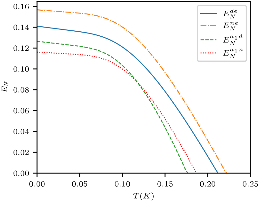
Figure 8: Line plots for $E_{N}^{de}$, $E_{N}^{ne}$, $E_{N}^{a_{1}d}$, and $E_{N}^{a_{1}n}$ as a function of temperature each considered at the optimized value of cavity detuning $\Delta_{a}$, effective magnon detuning $\tilde{\Delta}_{n}$, ensemble detuning $\Delta_{e}$, and cavity-cavity coupling rate $J$ as shown in Table 2.

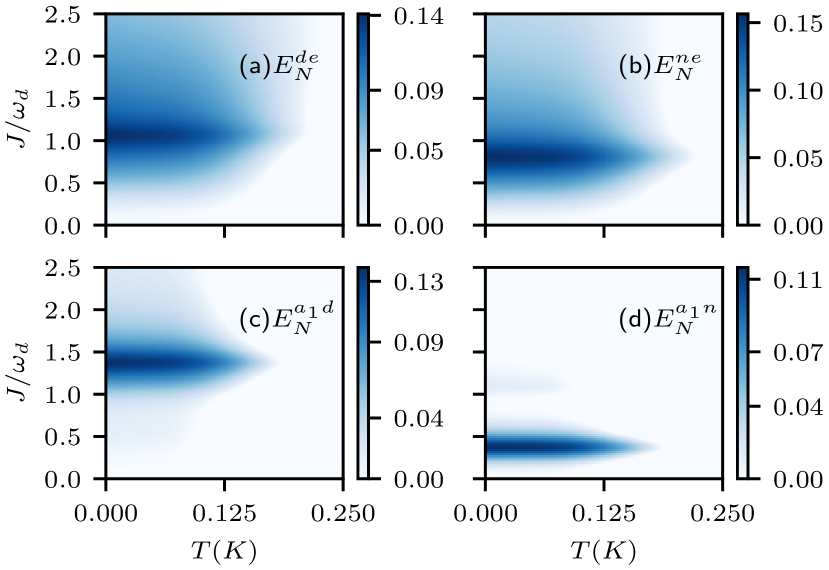
Figure 9: Density plot of (a) $E_{N}^{de}$, (b) $E_{N}^{ne}$ (c) $E_{N}^{a_{1}d}$, and (d) $E_{N}^{a_{1}n}$ as a function of temperature $T$ and normalized coupling rate $J/\omega_{d}$. Other parameters are optimized as shown in Table 2.

It is important to find how the strength of cavity-cavity coupling $J$ impacts the robustness of distant entanglement against temperature. In Fig. 9, we present density plots of $E_{N}^{de}$, $E_{N}^{ne}$, $E_{N}^{a_{1}d}$, and $E_{N}^{a_{1}n}$ as a function of temperature $T$ and cavity-cavity coupling $J$. We infer from Fig. 9 that $T_{c}$ for the existence of entanglement varies with $J$. The maximum value of $J$ corresponding to maximal $E_{N}^{de}$ [see Fig. 9(a)], $E_{N}^{ne}$ [see Fig. 9(b)], $E_{N}^{a_{1}d}$ [see Fig. 9(c)], and $E_{N}^{a_{1}n}$ [see Fig. 9(d)] is $1.2\,\omega_{d}$, $0.8\,\omega_{d}$, $1.28\,\omega_{d}$, and $0.35\,\omega_{d}$, respectively. We observe that $T_{c}$ is maximum corresponding to $J$ for which the degree of entanglement is maximal. Hence, we can say $T_{c}$ can be increased through a proper choice of parameters.

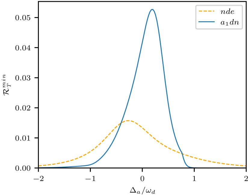
Figure 10: Tripartite entanglement of cavity 1 photon-magnon-phonon ($a_{1}dn$) and ensemble-magnon-phonon ($nde$) modes as a function of $\Delta_{a}/{\omega_{d}}=-\Delta_{1}/{\omega_{d}}=\Delta_{2}/{\omega_{d}}$ at $\Delta_{e}=2\,\omega_{d}$, $\tilde{\Delta}_{n}=0.25\,\omega_{d}$ for $a_{1}dn$ and $\Delta_{e}=-0.5\,\omega_{d}$, $\tilde{\Delta}_{n}=0.65\,\omega_{d}$ for $nde$ tripartite subsystems. Cavity-cavity coupling strength is $J=\omega_{d}$.

Apart from bipartite entanglement of different subsystems in coupled magnomechanical system, we show that genuine tripartite entanglement can also be realized for indirectly coupled subsystems. The same micromechanical system without cavity 1 was recently considered by Jie Li et al. [25] in which they showed that the tripartite magnon-phonon-photon entanglement exists when $\tilde{\Delta}_{n}\simeq 0.9\,\omega_{d}$ (stokes sideband) and $\Delta_{a}\simeq\omega_{d}$ (anti-stokes sideband). In the coupled magnomechanical system, we consider magnon-phonon-ensemble ($nde$) and cavity-1 photon-phonon-magnon ($a_{1}dn$) tripartite subsystems and plot the minimum of the residual contangle in Fig. 10 as a function of normalized detuning $\Delta_{a}/\omega_{d}$. Both these entanglements $nde$ and $a_{1}dn$ exist for a significant range of cavity field detuning with maximum values near resonant frequency. Interestingly, cavity-1 photon-phonon-magnon entanglement has approximatly the same degree of entanglement as found in single cavity case [25].
In the coupled cavity scheme, further investigations may incorporate the inclusion of cross-Kerr non-linearity [56], exploration of entanglement dynamics in ultra-strong coupling regime [57], study of Einstein-Podolsky-Rosen (EPR) steering [58], and the introduction of optical parametric amplifier(OPA) to widen the parametric regime for entanglement [59]. Furthermore, the noise induced decoherence can be curtailed by purification and entanglement concentration in a practical long-distance quantum communication network [60, 61].

IV Conclusion

We have suggested a potential scheme consisting of two microwave cavities coupled to each other housing an atomic ensemble and a YIG sphere. We have investigated continuous variable entanglement between disparate physical systems. We have shown that bipartite entanglement between ensemble, phonon, and magnon modes not only exists, but it can sustain itself up to $200\,$mK temperature, corresponding to a proper choice of experimentally feasible parameters. In addition, photon and magnon modes can also be entangled with cavity-1 photons and their entanglement is robust against temperature of about $170\,$mK. Furthermore, we have demonstrated parameters for which significant tripartite entanglement of magnon-phonon-ensemble and cavity-1 photon-phonon-magnon subsystems exist. Hence, we conclude that both the bipartite and tripartite entanglement between indirectly coupled systems are found to be substantial in our proposed setup. Moreover, cavity-cavity coupling strength plays a key role in the degree of entanglement as well as the range of parameters in which it subsists. This scheme may prove to be significant for processing continuous variable quantum information in quantum memory protocols.

References

- Horodecki et al. [2009] R. Horodecki, P. Horodecki, M. Horodecki, and K. Horodecki, Quantum entanglement, Reviews of Modern Physics 81, 865 (2009).
- Fröwis et al. [2018] F. Fröwis, P. Sekatski, W. Dür, N. Gisin, and N. Sangouard, Macroscopic quantum states: Measures, fragility, and implementations, Rev. Mod. Phys. 90, 025004 (2018).
- Kimble [2008] H. J. Kimble, The quantum internet, Nature 453, 1023 (2008).
- Simon [2017] C. Simon, Towards a global quantum network, Nature Photon 11, 678 (2017).
- Møller et al. [2017] C. B. Møller, R. A. Thomas, G. Vasilakis, E. Zeuthen, Y. Tsaturyan, M. Balabas, K. Jensen, A. Schliesser, K. Hammerer, and E. S. Polzik, Quantum back-action-evading measurement of motion in a negative mass reference frame, Nature 547, 191 (2017).
- Lukin et al. [2001] M. Lukin, M. Fleischhauer, and A. Imamoğlu, Quantum Information Processing Based on Cavity QED with Mesoscopic Systems, in Directions in Quantum Optics, edited by H. J. Carmichael, R. J. Glauber, and M. O. Scully (Springer Berlin Heidelberg, Berlin, Heidelberg, 2001).
- Aspelmeyer et al. [2014] M. Aspelmeyer, T. J. Kippenberg, and F. Marquardt, Cavity optomechanics, Rev. Mod. Phys. 86, 1391 (2014).
- Favero and Marquardt [2014] I. Favero and F. Marquardt, Focus on optomechanics, New Journal of Physics 16, 085006 (2014).
- Favero and Karrai [2009] I. Favero and K. Karrai, Optomechanics of deformable optical cavities, Nature Photonics 3, 201 (2009).
- Meystre [2013] P. Meystre, A short walk through quantum optomechanics, Annalen der Physik 525, 215 (2013).
- Wang and Clerk [2012] Y.-D. Wang and A. A. Clerk, Using dark modes for high-fidelity optomechanical quantum state transfer, New Journal of Physics 14, 105010 (2012).
- Mari and Eisert [2012] A. Mari and J. Eisert, Opto- and electro-mechanical entanglement improved by modulation, New Journal of Physics 14, 075014 (2012).
- Sangouard et al. [2011] N. Sangouard, C. Simon, H. de Riedmatten, and N. Gisin, Quantum repeaters based on atomic ensembles and linear optics, Rev. Mod. Phys. 83, 33 (2011).
- Tabuchi et al. [2014] Y. Tabuchi, S. Ishino, T. Ishikawa, R. Yamazaki, K. Usami, and Y. Nakamura, Hybridizing Ferromagnetic Magnons and Microwave Photons in the Quantum Limit, Phys. Rev. Lett. 113, 083603 (2014).
- Huebl et al. [2013] H. Huebl, C. W. Zollitsch, J. Lotze, F. Hocke, M. Greifenstein, A. Marx, R. Gross, and S. T. B. Goennenwein, High Cooperativity in Coupled Microwave Resonator Ferrimagnetic Insulator Hybrids, Phys. Rev. Lett. 111, 127003 (2013).
- Wang et al. [2020] L. Wang, Z. Lu, X. Zhao, W. Zhang, Y. Chen, Y. Tian, S. Yan, L. Bai, and M. Harder, Magnetization coupling in a YIG/GGG structure, Phys. Rev. B 102, 144428 (2020).
- Goryachev et al. [2014] M. Goryachev, W. G. Farr, D. L. Creedon, Y. Fan, M. Kostylev, and M. E. Tobar, High-Cooperativity Cavity QED with Magnons at Microwave Frequencies, Phys. Rev. Applied 2, 054002 (2014).
- Bai et al. [2015] L. Bai, M. Harder, Y. Chen, X. Fan, J. Xiao, and C.-M. Hu, Spin Pumping in Electrodynamically Coupled Magnon-Photon Systems, Phys. Rev. Lett. 114, 227201 (2015).
- Hisatomi et al. [2016] R. Hisatomi, A. Osada, Y. Tabuchi, T. Ishikawa, A. Noguchi, R. Yamazaki, K. Usami, and Y. Nakamura, Bidirectional conversion between microwave and light via ferromagnetic magnons, Phys. Rev. B 93, 174427 (2016).
- Osada et al. [2016] A. Osada, R. Hisatomi, A. Noguchi, Y. Tabuchi, R. Yamazaki, K. Usami, M. Sadgrove, R. Yalla, M. Nomura, and Y. Nakamura, Cavity Optomagnonics with Spin-Orbit Coupled Photons, Phys. Rev. Lett. 116, 223601 (2016).
- Haigh et al. [2016] J. Haigh, A. Nunnenkamp, A. Ramsay, and A. Ferguson, Triple-Resonant Brillouin Light Scattering in Magneto-Optical Cavities, Phys. Rev. Lett. 117, 133602 (2016).
- Lachance-Quirion et al. [2017] D. Lachance-Quirion, Y. Tabuchi, S. Ishino, A. Noguchi, T. Ishikawa, R. Yamazaki, and Y. Nakamura, Resolving quanta of collective spin excitations in a millimeter-sized ferromagnet, Science Advances 3, e1603150 (2017).
- Wang et al. [2018] Y.-P. Wang, G.-Q. Zhang, D. Zhang, T.-F. Li, C.-M. Hu, and J. You, Bistability of Cavity Magnon Polaritons, Phys. Rev. Lett. 120, 057202 (2018).
- Tabuchi et al. [2015] Y. Tabuchi, S. Ishino, A. Noguchi, T. Ishikawa, R. Yamazaki, K. Usami, and Y. Nakamura, Coherent coupling between a ferromagnetic magnon and a superconducting qubit, Science 349, 405 (2015).
- Li et al. [2018] J. Li, S.-Y. Zhu, and G. Agarwal, Magnon-Photon-Phonon Entanglement in Cavity Magnomechanics, Phys. Rev. Lett. 121, 203601 (2018).
- Li and Zhu [2019] J. Li and S.-Y. Zhu, Entangling two magnon modes via magnetostrictive interaction, New J. Phys. 21, 085001 (2019).
- Wu et al. [2021] W.-J. Wu, Y.-P. Wang, J.-Z. Wu, J. Li, and J. Q. You, Remote magnon entanglement between two massive ferrimagnetic spheres via cavity optomagnonics, Phys. Rev. A 104, 023711 (2021).
- Ning and Yin [2021] C.-X. Ning and M. Yin, Entangling magnon and superconducting qubit by using a two-mode squeezed-vacuum microwave field, J. Opt. Soc. Am. B, JOSAB 38, 3020 (2021).
- Wang et al. [2022] N. Wang, Z.-B. Yang, S.-Y. li, Y.-L. Tong, and A.-D. Zhu, Nonreciprocal transmission and asymmetric entanglement induced by magnetostriction in a cavity magnomechanical system, Eur. Phys. J. Plus 137, 422 (2022).
- Ren et al. [2022] Y.-l. Ren, J.-k. Xie, X.-k. Li, S.-l. Ma, and F.-l. Li, Long-range generation of a magnon-magnon entangled state, Phys. Rev. B 105, 094422 (2022).
- Chen [2013] Y. Chen, Macroscopic quantum mechanics: theory and experimental concepts of optomechanics, J. Phys. B: At. Mol. Opt. Phys. 46, 104001 (2013).
- Joshi et al. [2012] C. Joshi, J. Larson, M. Jonson, E. Andersson, and P. Öhberg, Entanglement of distant optomechanical systems, Phys. Rev. A 85, 033805 (2012).
- Akram et al. [2012] U. Akram, W. Munro, K. Nemoto, and G. J. Milburn, Photon-phonon entanglement in coupled optomechanical arrays, Phys. Rev. A 86, 042306 (2012).
- Ge et al. [2013] W. Ge, M. Al-Amri, H. Nha, and M. S. Zubairy, Entanglement of movable mirrors in a correlated-emission laser, Phys. Rev. A 88, 022338 (2013).
- Liao et al. [2014] J.-Q. Liao, Q.-Q. Wu, and F. Nori, Entangling two macroscopic mechanical mirrors in a two-cavity optomechanical system, Phys. Rev. A 89, 014302 (2014).
- Bai et al. [2016] C.-H. Bai, D.-Y. Wang, H.-F. Wang, A.-D. Zhu, and S. Zhang, Robust entanglement between a movable mirror and atomic ensemble and entanglement transfer in coupled optomechanical system, Scientific Reports 6, 33404 (2016).
- Li et al. [2020] G. Li, W. Nie, Y. Wu, Q. Liao, A. Chen, and Y. Lan, Manipulating the steady-state entanglement via three-level atoms in a hybrid levitated optomechanical system, Physical Review A 102, 063501 (2020).
- Ian et al. [2008] H. Ian, Z. R. Gong, Y.-x. Liu, C. P. Sun, and F. Nori, Cavity optomechanical coupling assisted by an atomic gas, Physical Review A 78, 013824 (2008).
- Zhou et al. [2011] L. Zhou, Y. Han, J. Jing, and W. Zhang, Entanglement of nanomechanical oscillators and two-mode fields induced by atomic coherence, Physical Review A 83, 052117 (2011).
- Genes et al. [2008a] C. Genes, D. Vitali, and P. Tombesi, Emergence of atom-light-mirror entanglement inside an optical cavity, Phys. Rev. A 77, 050307 (2008a).
- Hald et al. [1999] J. Hald, J. L. Sørensen, C. Schori, and E. S. Polzik, Spin Squeezed Atoms: A Macroscopic Entangled Ensemble Created by Light, Phys. Rev. Lett. 83, 1319 (1999).
- Zhang et al. [2016] X. Zhang, C.-L. Zou, L. Jiang, and H. X. Tang, Cavity magnomechanics, Science Advances 2, e1501286 (2016).
- Zheng [2012] S.-B. Zheng, Generation of atomic and field squeezing by adiabatic passage and symmetry breaking, Phys. Rev. A 86, 013828 (2012).
- Holstein and Primakoff [1940] T. Holstein and H. Primakoff, Field Dependence of the Intrinsic Domain Magnetization of a Ferromagnet, Phys. Rev. 58, 1098 (1940).
- Hammerer et al. [2010] K. Hammerer, A. S. Sørensen, and E. S. Polzik, Quantum interface between light and atomic ensembles, Rev. Mod. Phys. 82, 1041 (2010).
- Zhang et al. [2014] X. Zhang, C.-L. Zou, L. Jiang, and H. X. Tang, Strongly Coupled Magnons and Cavity Microwave Photons, Phys. Rev. Lett. 113, 156401 (2014).
- Clerk et al. [2010] A. A. Clerk, M. H. Devoret, S. M. Girvin, F. Marquardt, and R. J. Schoelkopf, Introduction to quantum noise, measurement, and amplification, Rev. Mod. Phys. 82, 1155 (2010).
- Genes et al. [2008b] C. Genes, A. Mari, P. Tombesi, and D. Vitali, Robust entanglement of a micromechanical resonator with output optical fields, Phys. Rev. A 78, 032316 (2008b), publisher: American Physical Society.
- DeJesus and Kaufman [1987] E. X. DeJesus and C. Kaufman, Routh-Hurwitz criterion in the examination of eigenvalues of a system of nonlinear ordinary differential equations, Phys. Rev. A 35, 5288 (1987).
- Unbehauen [2009] H. D. Unbehauen, Control Systems, Robotics and AutomatioN – Volume XII: Nonlinear, Distributed, and Time Delay Systems-I (EOLSS Publications, 2009).
- Plenio [2005] M. B. Plenio, Logarithmic Negativity: A Full Entanglement Monotone That is not Convex, Physical Review Letters 95, 090503 (2005).
- Vidal and Werner [2002] G. Vidal and R. F. Werner, Computable measure of entanglement, Phys. Rev. A 65, 032314 (2002).
- Simon and Horodecki [2000] R. Simon and P. Horodecki, Separability Criterion for Continuous Variable Systems, Phys. Rev. Lett. 84, 2726 (2000).
- Adesso and Illuminati [2006] G. Adesso and F. Illuminati, Continuous variable tangle, monogamy inequality, and entanglement sharing in Gaussian states of continuous variable systems, New J. Phys. 8, 15 (2006).
- Coffman et al. [2000] V. Coffman, J. Kundu, and W. K. Wootters, Distributed entanglement, Physical Review A 61, 052306 (2000).
- Sheng et al. [2008] Y.-B. Sheng, F.-G. Deng, and H.-Y. Zhou, Efficient polarization-entanglement purification based on parametric down-conversion sources with cross-Kerr nonlinearity, Phys. Rev. A 77, 042308 (2008).
- Teo and Gong [2013] Y. S. Teo and J. Gong, Double Rabi model in the ultra-strong coupling regime: entanglement and chaos beyond the rotating wave approximation, J. Phys. B: At. Mol. Opt. Phys. 46, 235504 (2013).
- Tan and Li [2021] H. Tan and J. Li, Einstein-Podolsky-Rosen entanglement and asymmetric steering between distant macroscopic mechanical and magnonic systems, Phys. Rev. Research 3, 013192 (2021).
- Hussain et al. [2022] B. Hussain, S. Qamar, and M. Irfan, Entanglement enhancement in cavity magnomechanics by an optical parametric amplifier, Phys. Rev. A 105, 063704 (2022).
- Bennett et al. [1996] C. H. Bennett, G. Brassard, S. Popescu, B. Schumacher, J. A. Smolin, and W. K. Wootters, Purification of Noisy Entanglement and Faithful Teleportation via Noisy Channels, Phys. Rev. Lett. 76, 722 (1996).
- Yamamoto et al. [2001] T. Yamamoto, M. Koashi, and N. Imoto, Concentration and purification scheme for two partially entangled photon pairs, Phys. Rev. A 64, 012304 (2001).