3inGAN: Learning a 3D Generative Model from Images of a Self-similar Scene

Abstract

We introduce 3inGAN, an unconditional 3D generative model trained from 2D images of a single self-similar 3D scene. Such a model can be used to produce 3D “remixes” of a given scene, by mapping spatial latent codes into a 3D volumetric representation, which can subsequently be rendered from arbitrary views using physically based volume rendering. By construction, the generated scenes remain view-consistent across arbitrary camera configurations, without any flickering or spatio-temporal artifacts. During training, we employ a combination of 2D, obtained through differentiable volume tracing, and 3D Generative Adversarial Network (GAN) losses, across multiple scales, enforcing realism on both its 2D renderings and its 3D structure. We show results on semi-stochastic scenes of varying scale and complexity, obtained from real and synthetic sources. We demonstrate, for the first time, the feasibility of learning plausible view-consistent 3D scene variations from a single exemplar scene and provide qualitative and quantitative comparisons against two recent related methods. Code and data for the paper are available at https://geometry.cs.ucl.ac.uk/group_website/projects/2022/3inGAN/.

1 Introduction

In the context of images, unconditional generative models, such as GANs, learn to map latent spaces to diverse yet realistic high resolution images – notable architectures include StyleGan [36] and BigGAN [9]. Furthermore, these models have been shown to contain high-level semantics in their latent space mappings, allowing powerful post-hoc image editing operations, such as changing the appearance and expression of a generated person [1, 56, 22]. One key question therefore, is whether it is possible to learn similar generative models for 3D scenes.

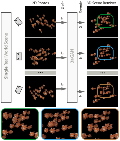
Figure 1: Single scene 3D remixes. We introduce 3inGAN that takes a set of 2D photos of a single self-similar scene to produce a generative model of 3D scene remixes, each of which can be rendered from arbitrary camera configurations, without any flickering or spatio-temporal artifacts. Bottom row insets show zooms from different generative samples, rendered from the same camera view, to highlight the quality and diversity of the results.

There are, however, two key challenges. First, 3D generation suffers from data scarcity as obtaining large and diverse datasets for 3D data, both geometry and appearance, is significantly more challenging than for 2D data, where one can simply scrape images from the internet. Second, generative models struggle as the domain complexity increases, as well as when datasets are not prealigned. This problem is even more severe in 3D, due to the added scene complexity, both in terms of scene structure and object appearance, and the fact that 3D models and scans often come with their own coordinate systems and/or scaling.

In this work, we propose 3inGAN, a solution to address both problems in a restrictive setting: an unconditional generative model for 3D scenes that works on a per-scene basis for self-similar configurations. As our method does not require a large 3D dataset during training, it could be used across a wide range of real world domains. By restricting the data domain to a single 3D scene, we simplify the unconditional generation problem space to one with limited domain complexity, allowing us to learn a high-quality generator. We were inspired by similar approaches proposed for 2D images, e.g., SinGAN [55]. However, extending such approaches to 3D is nontrivial, as in 3D, one must be able to generate arbitrary views in a way that is multi-view consistent. We handle this by directly generating a 3D scene representation that is, by definition, multiview consistent. In particular, we generate a regularly sampled nonlinearly-interpolated-voxel grid [31] due to its simplicity, local (feature) influence, rendering efficiency, and its amenability to the prevailing convolutional generator and discriminator architectures in 2D/3D. In order to achieve realism, both in terms of 3D structure and 2D image appearance, we simultaneously use 3D feature patches and 2D image patches to obtain gradients from the 3D and 2D discriminators, respectively. We link the 3D and 2D domains by using a differentiable volume rendering module to interpret the feature grid as RGB images. Note that recent neural 3D generators (e.g., BlockGAN [48], GRAF [54], $\pi$-GAN [10]) are trained on image/shape collections, and are not easily applicable in our setup (see Section 4 for comparison). For example, Fig. 1 shows a sampling of “remixed” results generated from images of a school of fish.

In summary, ours is the first work to introduce an unconditional generative model from a single 3D scene. In particular, we investigate scenes with some degree of stochastic structure, which are suitable to shuffling or “remixing” the scene content into a new 3D scene that makes sense. In addition, we make a further simplifying assumption in that we drop the view-specific effects and reconstruct Lambertian scenes. We evaluate our proposed method on a series of synthetic and real scenes and show that our approach outperforms baselines in terms of quality and diversity.

2 Related Work

2D generative models.  Generative modeling for image synthesis learns a distribution of colour values over the pixels of an image, and has seen tremendous progress recently, with GANs being the de-facto standard for synthesizing realistic looking images [33, 36, 37, 9, 32]. Recent works such as [34] further improve result quality in data-sparse regimes, while [35] applies signal processing techniques to the generator architecture to correct for aliasing errors. Other contenders for generative modelling include VAEs [60, 2, 40, 26], flow-based models [39, 15, 14], noise-diffusion based models [57, 58, 29, 4], and even hybrids of these methods [51, 4, 18, 41]. Key to training such methods is the availability of large scale image collections, and often times such works are used on specific target domains, such as portrait photos.

More similar to ours, Single Image GANs (SinGANs) [55, 27] learn to generate the distribution of patches of a single image, in a progressive coarse-to-fine manner so as to generate plausible variations from that one single image. Such approaches avoid the problem of needing a large dataset, while still enabling useful applications such as retargetting. However, they are restricted to repeated, or stochastic-like patch-based variations. Ours shares similar advantages, as well as restrictions in terms of scene type as SinGAN. In Section 4 we show that a naïve extension to 3D volumes does not produce reasonable results.

3D generative models.  Due to the lack of large scale real-world datasets, much of the research in 3D generative modeling has stayed in the synthetic realm such as modeling only 3D shapes [62, 45, 8, 7, 12, 16], or materials [21]. Other methods use synthetic datasets for predicting scene structure and use differentiable rendering for end-to-end training [66, 38, 50, 30]. Recently, methods that directly model 3D scenes, either using explicit or implicit neural scene representations, have been gaining popularity [25, 47, 10, 54, 49, 13, 67, 19]. Another successful line of work [47, 49] uses a neural renderer to render features from a volumetric grid, followed by per-image 2D CNNs used for upsampling, and as such are not multiview consistent. In contrast, [10, 54] and [13] are view-consistent by design since they use an implicit neural representation and explicit-implicit neural representation respectively for the 3D structure, using a physically based rendering equation for obtaining the final 2D images. Concurrent works such as [67, 19] produce impressive results performing 3D synthesis with multi-view consistency. Such approaches are designed to be trained only through 2D (image) supervision, and work best in cases where large datasets can be obtained for limited domains, such as faces or cars. Our method is also 3D view-consistent by design, and can be applied on a long-tail of real world scenes, provided they are self-similar.

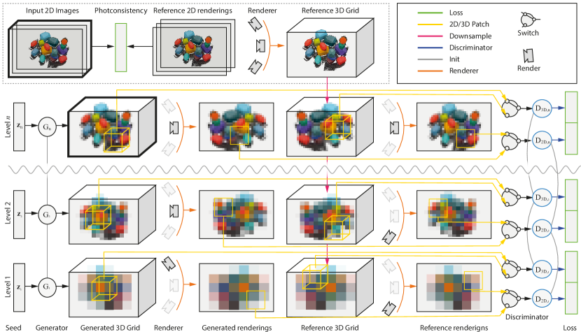
Figure 2: 3inGAN setup. Overview of our approach with two parts: an initialization of a reference 3D feature grid (top) and a stage-wise learning of a generative model (bottom). Input to the system is a set of 2D images seen on the top left. From these, optimization using differentiable rendering for known views produces the reference feature grid, which is the input to the next step. The rows below (“Level”) denote levels of training the generator, a 2D discriminator, and a 3D discriminator. The 3D discriminator (right) gets random 3D patches from the reference or generated 3D grid, while the 2D discriminator (right) gets random 2D patches from reference or from generated renderings.

Differentiable rendering.  Differentiable rendering [59] enables neural networks to be trained by losses on the resulting rendered images of a 3D representation, by allowing the gradient to be back-propagated through the network. This has shown to be a highly effective tool, especially for learning 3D representations that allow for novel view synthesis. Multiple works [28, 46, 3, 61, 43, 68] have focused on designing neural-networks, either convolutional or otherwise, to go from spatial features to rendered pixels. Lately, methods that use volume tracing have been favored due to the advantage of flicker-free 2D rendering by design. Neural Radiance Fields [44] were the first to introduce this way of using differentiable rendering while using a neural 3D scene representation. Subsequently, many extensions of this have been proposed, to increase quality, robustness to scene type, or rendering speed [44, 65, 6, 64, 11, 17, 63, 23, 52, 20]. Although using an MLP to learn a continuous scene representation has been shown to be able to lead to very high quality view synthesis results, such MLPs are not amenable in the generative contexts as ours, as explained next.

3 Our Approach

Motivation.  As input, we require an exemplar self-similar scene, which is provided as a set of posed 2D images. We desire that our method produces a plausible 3D scene structure that matches the exemplar scene on a patch basis, and realistic 2D image renderings that are consistent across the space of all views of that scene.

Given this goal, we choose to directly generate a 3D representation, so that we are guaranteed view consistency when rendering 2D images from it. The first question is, what 3D representation should we use? One choice would be coordinate-based MLPs, which have been shown to be compact scene representations able to generate very high quality novel views [44]. However, such a representation is ill-suited for a generative setup, as the costly evaluation makes rendering volumetric and image patches in the training loop infeasible, and the global and distributed nature of the MLP representation makes GAN training challenging in our patch-based setting. Another option is to operate directly on discretized RGBA volumes but, as demonstrated in Karnewar et al. [31], such an approach results in limited quality (blurry) results. Instead, we build our approach using their proposed grid-based ReLU Field representation. This representation is detailed in brief in section 3.1.

A naïve extension of SinGAN [55] to 3D fails to produce good results for multiple reasons: (i) only using a 3D discriminator doesn’t have the notion of free-space in the volume and also tries to replicate the inside regions of the occupied space that may contain random values. When such a model is rendered, the results have minor shape distortions and chromatic noise; (ii) only using 2D discriminators on the rendered images is challenging. Specifically, when trained on too small patches the discriminator becomes too weak to inform the generator, and when trained on too large patches, the generator simply memorizes the initial reconstruction. Our solution involves two main ingredients: the use of ReLU-Fields representation [31] instead of the standard RGBA volumes for inherently inducing the notion of free space in the 3D-grid; and a mixture of 2D and 3D discriminators, along with multi-scale training, that robustly produce consistent and high quality reconstructions.

Method overview.  Input to our method is a set of ${n_{\mathrm{2D}}}$ 2D images $\mathcal{I}:=\{I_{1},\ldots,I_{n_{\mathrm{2D}}}\}$ taken from one real world or synthetic self-similar scene. Fig. 2 presents a graphical overview and Alg. 1 a pseudo-code version. Our method consists of two main steps. First, we convert the 2D image set into a 3D feature grid $V$ (Sec. 3.1). Then, we train a generative model $G$ of 3D scenes from this 3D feature grid and its 2D rendered images (Sec. 3.2). This generative model $G(\mathbf{z})$ then converts spatial random latent grids ($\mathbf{z}$ ) into 3D feature grids containing remixes of the exemplar scene, which can be consistently rendered from arbitrary views.

Algorithm 1 Our 3inGAN training. Function $\mathtt{sample}(\ldots)$ samples all distributions provided as arguments; $\mathtt{up}(a,b)$ ADAM-updates the parameters $a$ by the gradient of expression $b$ with respect to $a$.

1:repeat$\triangleright$ 3D representation building

2:     $\{I,\mathsf{C}\}:=\mathtt{sample}(\mathcal{I},\mathcal{C})$

3:     $V:=\mathtt{up}(V,\|\mathcal{R}(V,\mathsf{C})-I\|^{2}_{2})$

4:until converged.

5:repeat$\triangleright$ Generator training

6:     $\{\mathbf{z},\mathsf{C}\}:=\mathtt{sample}(\mathcal{N},\mathcal{D})$

7:     $P:=\mathcal{P}_{\mathrm{2D}}(\mathcal{R}(G^{\theta}(\mathbf{z}),\mathsf{C}))$

8:     $\phi:=\mathtt{up}(\phi,D_{\mathrm{2D}}^{\phi}(P=\mathtt{fake}))$

9:     $\mathsf{C}:=\mathtt{sample}(\mathcal{D})$

10:     $P:=\mathcal{P}_{\mathrm{2D}}(\mathcal{R}(V,\mathsf{C}))$

11:     $\phi:=\mathtt{up}(\phi,D_{\mathrm{2D}}^{\phi}(P=\mathtt{real}))$

12:     $\mathbf{z}:=\mathtt{sample}(\mathcal{N})$

13:     $P:=\mathcal{P}_{\mathrm{3D}}(G^{\theta}(\mathbf{z}))$

14:     $\psi:=\mathtt{up}(\psi,D_{\mathrm{3D}}^{\psi}(P=\mathtt{fake}))$

15:     $P:=\mathcal{P}_{\mathrm{3D}}(V)$

16:     $\psi:=\mathtt{up}(\psi,D_{\mathrm{3D}}^{\psi}(P=\mathtt{real}))$

17:     $\{\mathbf{z},\mathsf{C}\}:=\mathtt{sample}(\mathcal{N},\mathcal{D})$

18:     $\theta:=\mathtt{up}(\theta,D_{\mathrm{2D}}^{\phi}(\mathcal{P}_{\mathrm{2D}}(\mathcal{R}(G^{\theta}(\mathbf{z}),\mathsf{C}))=\mathtt{real}))$

19:     $\theta:=\mathtt{up}(\theta,D_{\mathrm{3D}}^{\psi}(\mathcal{P}_{\mathrm{3D}}(G^{\theta}(\mathbf{z}))=\mathtt{real}))$

20:until converged.

3.1 Representation

Foreground ReLU Field [31].  Foreground is bound by a user-provided Axis-Aligned Bounding Box (AABB) covered by a volumetric grid, $V$ , of fixed resolution ${n_{\mathrm{V}}}_{x}\times{n_{\mathrm{V}}}_{y}\times{n_{\mathrm{V}}}_{z}$ to contain feature values in the $[-1,1]$ range. These values correspond to the raw-features that are stored on the voxel-grid. In order to obtain continuous density field, the trilinearly interpolated values of these raw features are passed through a single channel-wise Rectified Linear Unit (ReLU) to convert them to $[0,1]$ range which can be physically interpreted as the density values. We do not model view-dependent appearance, i.e., we approximate the scene with Lambertian materials.

Background.  The background is assumed to be constant black for synthetic scenes. For real scenes, we model the background of the scene using an implicit neural network $B$ , similar to NeRF++ [65], but without using the inverted-sphere parametrization of the scene. Our goal is not to model the entire scene perfectly, but rather to provide appropriate inductive bias to the reconstruction pipeline to do the foreground-background separation correctly. This allows us to reconstruct real-world scenes without the requirement of additional segmentation masks.

Optimization.  Let the camera pose (extrinsic translation and rotation as well as intrinsics) for each input image be $\mathcal{C}:=\{\mathsf{C}_{1},\ldots,\mathsf{C}_{n_{\mathrm{2D}}}\}$ and assume they are known, e.g., by using structure-from-motion (we use ColMap [53]). Further, we denote the rendering operation to convert the feature grid $V$ and the camera pose $\mathsf{C}$ into an image as $\mathcal{R}(V,\mathsf{C})$. Specifically, we use emission-absorption raymarching [42, 25]. See supplementary for more details for the rendering. We can then directly optimize the feature grid’s photometric loss, given the pose and the 2D images as,

$$\operatorname{arg\,min}_{V}\sum_{i=1}^{n_{\mathrm{2D}}}\|I_{i}-\mathcal{R}(V,\mathsf{C}_{i})\|^{2}_{2}.$$ (1)

We minimize with batched optimization over 2048 random rays out of all the rays for which we know the 2D input image pixel value. Input images are of size $512\times 512$. Further, instead of directly optimizing for the full-resolution volume $V$ , training proceeds progressively in a coarse-to-fine manner. Initially, the feature grid is optimized at a resolution where each dimension is smaller by factor 16. After seeing 20k batches of input rays, the feature grid resolution is multiplied by two and the feature grid tri-linearly upsampled.

3.2 Generation

Training the generative model makes use of the 3D feature grid $V$ trained in the previous section 3.1, which we denote as the reference grid herein. We look into the generator details first, before explaining the losses used to train it: 2D and 3D discriminators, and a 2D and 3D reconstruction loss.

Generator.  Recall, that the model $G$ maps random latent codes $\mathbf{z}$ to a 3D feature grid $G(\mathbf{z})$ at the coarsest stage. While adds fine residual details to previous stage’s outputs at the rest of the stages similar to SinGAN [55]. The generator is a 3D CNN that stagewise decodes a spatial grid of noise vectors $\mathbf{z}$ of size $n_{\mathrm{z}}$ (we use $seedDimension=4$) into the grid of the desired resolution.

Training.  We train the architecture progressively: the generator first produces grids of reduced resolution. Only once this has converged, layers are added and the model is trained to produce the higher resolution. Note that we freeze the previously trained layers in order to avoid the GAN training from diverging. We employ an additional reconstruction loss that enforces one single fixed seed $\mathbf{z}^{\star}$ to map to the reference grid. We supervise this fixed seed loss via an MSE over the 3D grids and with 2D rendered patches.

2D discriminator.  A 2D loss discriminates 2D patches of renderings of the generated feature grid to 2D patches rendered from the reference grid $V$ . To render the 3D grids we need to model another distribution of poses, denoted by $\mathcal{D}$ , that uniformly samples camera locations to point at the center of the hemisphere and where focal length is varied stagewise linearly, where the value at the final stage corresponds to the actual camera intrinsics.

Further, let $\mathcal{P}_{\mathrm{2D}}()$ be an operator to extract a random patch from a 2D image, with discriminators,

$$p_{\mathrm{F}}^{\mathrm{2D}}=\mathcal{P}_{\mathrm{2D}}(\mathcal{R}(G(\mathbf{z}),\mathcal{D}))\text{\; and \;}p_{\mathrm{R}}^{\mathrm{2D}}=\mathcal{P}_{\mathrm{2D}}(\mathcal{R}(V,\mathcal{D})).$$ (2)

Note, that we did not define $p_{\mathrm{R}}^{\mathrm{2D}}=\mathcal{P}_{\mathrm{2D}}(\mathcal{I})$, as this would limit ourselves to use real samples only from the limited set of known 2D image patches. “Trusting” our reference 3D feature grid has been extracted properly, we can instead sample it from arbitrary views and get a much richer set.

3D discriminator.  The 3D discriminator compares 3D patches from the generated feature grid to 3D patches of the reference feature grid. Let $\mathcal{P}_{\mathrm{3D}}(V)$ be an operator to extract a random patch from a 3D feature grid $V$ . The distributions to discriminate are,

$$p_{\mathrm{F}}^{\mathrm{3D}}=\mathcal{P}_{\mathrm{3D}}(G(\mathbf{z}))\text{\;\; and \;\;}p_{\mathrm{R}}^{\mathrm{3D}}=\mathcal{P}_{\mathrm{3D}}(V).$$ (3)

Finally, we use Wasserstein GAN [5] to both distributions as well as the reconstruction losses (in both 2D and 3D),

$$\mathcal{L}=\gamma_{\mathrm{2D}}\cdot \mathtt{wgan}(p_{\mathrm{R}}^{\mathrm{3D}},p_{\mathrm{F}}^{\mathrm{3D}})+\gamma_{\mathrm{3D}}\cdot\mathtt{wgan}(p_{\mathrm{R}}^{\mathrm{2D}},p_{\mathrm{F}}^{\mathrm{2D}})+$$ (4)

$$\rho_{\mathrm{2D}}\cdot \mathbb{E}_{\mathsf{C}\in\mathcal{D}}[\|\mathcal{R}(G(\mathbf{z}^{\star}),\mathsf{C})-\mathcal{R}(V,\mathsf{C})\|_{2}^{2}]+$$

$$\rho_{\mathrm{3D}}\cdot \|G(\mathbf{z}^{\star})-V\|_{2}^{2},$$

weighted by two pairs of two factors $\gamma_{\mathrm{2D}}$ , $\gamma_{\mathrm{3D}}$ and $\rho_{\mathrm{2D}}$ , $\rho_{\mathrm{3D}}$ . In practice, we use $\gamma_{\mathrm{2D}}=\gamma_{\mathrm{3D}}=1.0$ and as well as $\rho_{\mathrm{2D}}=\rho_{\mathrm{3D}}=10$.

4 Evaluation

We perform quantitative and qualitative evaluations of our approach on a number of different scenes, on which we compare to baseline methods, and evaluate design choices via an ablation study.

Comparisons and ablations.  We compare to four methods (Tab. 1). Besides our full method 3inGAN (Ours), we study two prior approaches and two ablations.

As there is no existing method for 3D single scene remixing, we instead compare to two recent methods that were designed to learn a 3D generative model for classes of objects, trained on a dataset of images/renderings where each image corresponds to a different instance and view, PiGAN [10] and Graf [54]. In these baselines, we test how well such methods work when given instead, many rendered views of a single scene. In both cases, we use the code provided by the authors and their recommended parameter settings. We mark whether the original approach was designed for a single scene or not in the last column in Tab. 1.

In the first ablation, our 2D only ablation, we evaluate the importance of the 3D discriminator and 3D reconstruction seed losses by running a version of our method with those losses removed, i.e. ($\rho_{\mathrm{3D}}=\gamma_{\mathrm{3D}}=0$ in Eq. 4). We refer to this method as OursPlatoGAN, as its GAN loss setting, which is only on the rendered 2D images, is similar to the setup used in Henzler et al. [25], while being applied on only a single scene.

In the second ablation, our 3D only ablation, we evaluate the importance of the 2D discriminator and 2D reconstruction seed loss, which we refer to as OursSinGAN3D. This approach is a naïve extension of SinGAN [55] to 3D. In other words, it is our approach without any differentiable rendering, i.e., with the 2D discriminator and 2D reconstruction seed losses removed ($\gamma_{\mathrm{2D}}=\rho_{\mathrm{2D}}=0$). Please see the supplementary material for further ablations of the reconstruction seed losses.

Figure 3: Datasets. Example renderings of the scenes from our synthetic and real world datasets (Blocks, Chalk).

Table 1: Comparisons and ablations. We enumerate the different methods based on how they make use of 2D versus 3D information, and if they operate on a single scene or multiple scenes.

	Disc.		Recon.		Single scene
	2D	3D	2D	3D
PiGAN [10]	✓	✕	✕	✕	✕
Graf [54]	✓	✕	✕	✕	✕
OursPlatoGAN	✓	✕	✓	✕	✓
OursSinGAN3D	✕	✓	✕	✓	✓
Ours	✓	✓	✓	✓	✓

Scenes.  We consider a mix of synthetic and real scenes, with various levels of stochasticity (a requirement for patch-based remixing of scenes). These scenes include a synthetic scene rendered from Blender showing fishes with the same orientation (Fish) as well as with random orientations (FishRot), a scene composed of 3D balloons (Balloons), inspired by [55]. We also use four semi-synthetic scenes that were real scenes reconstructed from images using photogrammetry and then cleaned by an artist and sold on SketchFab: a pile of dirt (DirtPile), a log pile (Logs), and a bush (Plants). We also make a fully synthetic (Forest) scene which has a ground plane so as to resemble most real-world settings. Finally, we include two real scenes with background for which we have no ground truth 3D available, which both show a random arrangement of geometric toys (Blocks) or pieces of colored chalks (Chalk). Note that in all the cases, regardless of the source, our method only accesses 2D renderings/images of the scene, not the 3D scene.

Evaluation metric.  We evaluate our method along two axes – visual quality, and scene diversity. With traditional 2D GANs, these are most commonly evaluated using FID. However, this metric is typically used over two datasets of images, whereas our situation is slightly different; we have only one ground truth scene, and a diverse distribution of generated scenes. We extend Single Image (SIFID) [55] to 3D, and also explicitly separate quality and diversity to separately compare along each axis.

Visual quality is measured as the expectation of SIFID scores between the distribution of exemplar 2D images and the distribution of rendered generated 2D images for a fixed camera over multiple seeds. We compute this expectation by taking a mean over a number of camera-views. This is similar in sprit to SIFID, except we compute it over images rendered from different views of the 3D scenes. Lower distance reflects better quality.

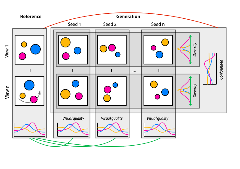
Figure 4: Single Image FID. We extend FID scores to our single scene use case. The distribution of feature responses is computed for different camera views (rows) and generations (columns) The reference (left) leads to a certain distribution of features. Rather than matching the reference distribution across all views and all seeds (red lines), we compare it to the distribution of a single fixed seed across all views (green lines) to measure visual quality. Then, we compare the variance of the distribution of features across all seeds under a fixed view as a measure of scene diversity.

Unfortunately, in the single scene case, we cannot meaningfully compute FID scores between the exemplar patch distribution and the distribution of all generated patches across seeds as it would make diversity appear as a distribution error. This is different from a typical GAN setup where we are given real images as samplings of desirable distribution of both quality and diversity. Instead, we measure scene diversity as the variance of a fixed patch from a fixed view over random seeds, which is a technique used to study texture synthesis diversity [24]. Larger diversity is better.

Table 2: Quality versus diversity. A good generative model should have a good mix of quality and diversity – excellent quality with no diversity or vice versa are both undesirable. Visual Quality and Scene Diversity for different methods (columns) and different data sets (rows). To simplify comparison, we normalize the numbers so that ours is always $1$. The best for each metric on each dataset is bolded and second best is underlined. Please refer to the supplementary for unscaled numbers.

	PiGAN [10]		Graf [54]		OursPlatoGAN		OursSinGAN3D		Ours
	Qual. $\downarrow$	Div. $\uparrow$	Qual. $\downarrow$	Div. $\uparrow$	Qual. $\downarrow$	Div. $\uparrow$	Qual. $\downarrow$	Div. $\uparrow$	Qual. $\downarrow$	Div. $\uparrow$
Fish	15.74	0.261	264.27	0.359	465.47	2.282	8.98	0.332	1.00	1.000
FishR	2.47	0.440	3.07	1.018	46.02	2.499	2.70	0.170	1.00	1.000
Balloons	1.44	0.024	3.25	0.477	1.79	0.482	9.57	0.083	1.00	1.000
Dirt	0.96	0.264	1.69	0.440	0.66	0.131	6.06	0.164	1.00	1.000
Forest	1.33	0.473	1.69	0.801	0.70	0.883	2.14	0.439	1.00	1.000
Plants	5.99	0.261	6.56	0.648	12.81	0.144	9.15	0.326	1.00	1.000
Blocks	0.91	0.224	0.73	0.342	1.83	0.334	3.32	0.329	1.00	1.000
Chalk	0.02	0.061	0.01	0.320	0.54	0.088	0.85	0.035	1.00	1.000

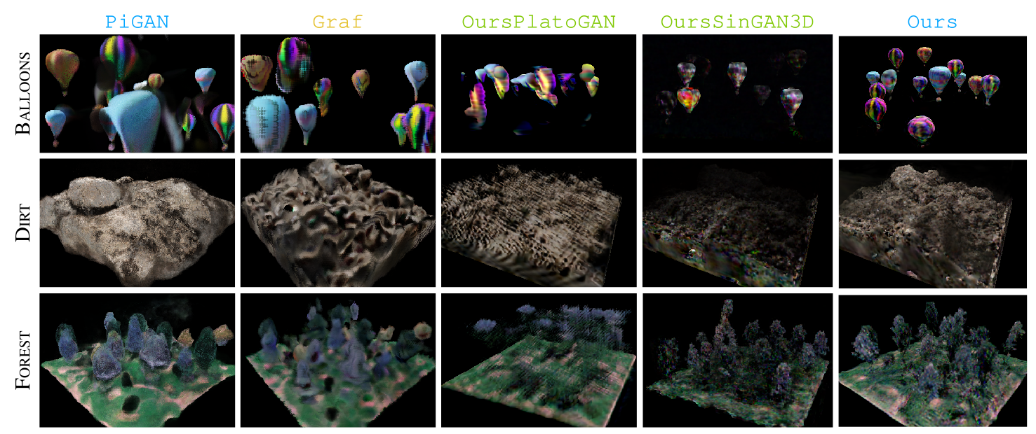
Figure 5: Qualitative comparison. Comparison of visual quality for different methods (columns) for different scenes (rows).

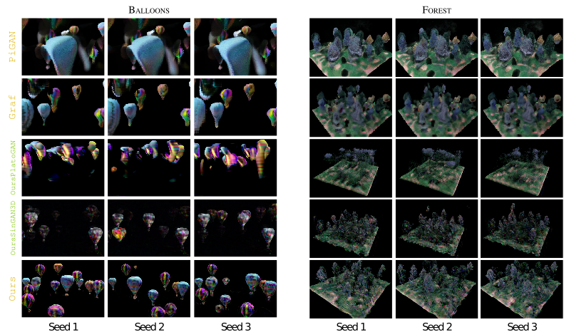
Figure 6: Diversity across different generative samples. Diversity under changing seeds (columns) of different methods (rows) for different scenes (left and right blocks). See also Figure 1.

4.1 Qualitative Evaluation

In Fig. 5 and Fig 6, we present qualitative results of 3inGAN, prior methods, and ablations. Please see the supplementary material for video results that can better visually demonstrate the quality and diversity of reconstructed scenes. We can see that, by construction, our method produces variations of 3D scenes that are view consistent.

Visual quality.  While some artifacts remain, we observe that this task is challenging for all existing approaches, and when compared to prior work and simple baselines, our method achieves higher visual quality. As expected, scenes with higher stochasticity result in better visual quality and diversity. For example, the balloons are mostly intact but shifted to different locations, and the dirt pile consists largely of reasonable structures.

Scene diversity.  Compared to the competing baselines, PiGAN and Graf, we observe that 3inGAN obtains significantly more scene diversity. This is not surprising, as prior methods have been designed to work on multi-scene image collections, and hence experience mode collapse when given views of only a single scene. This motivates the development of a patch-based generative model for 3D scenes. We see that 3inGAN learns to keep the identity of objects (e.g., balloons, fish, chalk) and create plausible 3D variations (e.g., balloons floating in air, or blocks meaningfully stacked). Please refer to the supplementary for more results.

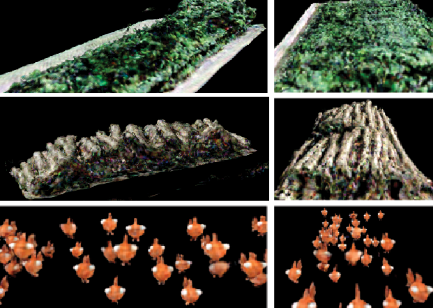
Figure 7: Scene retargetting. Retargeting the Plants, the Logs, and Fish scenes to novel aspect ratios. Since ours is CNN-based, it is easy to retarget scenes to different sizes.

Scene retargeting.  In Fig. 7 we show results of changing the aspect ratio of generated scenes. As our generator is fully convolutional, this can be done simply by changing the shape of the input noise. We can see that the scene structure remains plausible, with the semi-stochastic content repeated to fill in the space.

4.2 Quantitative Evaluation

In Tab. 2, we quantitatively compare the different variations using our proposed metrics. Mirroring the qualitative observations, we can see that 3inGAN performs better than prior work and ablations in terms of visual quality. The numbers show the importance of having both the 2D and 3D discriminators as they help to improve the object appearance and geometric structure, respectively, of the generations. Our main advantage is the noticeable boost in diversity of the generated results, as also measured in the 2–5$\times$ boost in scene diversity score over the other methods. Note that as indicated by the relative Visual Quality scores, our results are not yet close to being photorealistic (indistinguishable from the reference distribution) but nonetheless we achieve a healthy gain in over quality/diversity over competing alternatives.

5 Discussion

Limitations and future work.  Our approach has a number of limitations. For one, we note that the proposed method of generating a distribution (i.e., a generative model) from a single scene only makes sense in case where scenes contain stochastic structures that can be shuffled around. We do not expect our method to work on highly structured content, e.g., people. Furthermore, we observe that results can still exhibit artifacts, such as high frequency noise, blobby output, and floaters. We believe that this is because the scene distribution is being estimated from very limited data (i.e., a single scene), and is analogous to the “splotchyness” commonly seen in 2D GANs when trained in limited data settings or over complex distributions. In this case, it should be possible to improve quality by using data augmentation as recommended in [34], or by improving the training regime, as in [27], however in the latter case it is important to balance diversity to avoid mode collapse. Finally, in our implementation, we assume scenes to be Lambertian, i.e., without view-dependent effects. In the future, view-dependent specular effects could be modelled using SH components.

Conclusion.  We have presented 3inGAN, a method for training a generative model of remixes of a single 3D scene. Similar to SinGAN, our approach works on “long-tail” data, as it does not require aligned 3D datasets for training. Instead, we require only a set of posed images of a single self-similar scene as input. We believe that this method has a number of downstream applications, such as retargeting or harmonization [55], and furthermore, studies in generative models for 3D scenes may, one day, lead to realistic view-consistent scene generation on par with images. This would be practical not only for 3D content generation, but as a generative prior to be used in many 3D reconstruction and editing tasks.

Acknowledgements.

The work was partially supported by the Marie Skłodowska-Curie grant agreement No. 956585, gifts from Adobe, and the UCL AI Centre.

References

- [1] Rameen Abdal, Peihao Zhu, Niloy J Mitra, and Peter Wonka. Styleflow: Attribute-conditioned exploration of stylegan-generated images using conditional continuous normalizing flows. ACM Trans. Graph., 40(3):1–21, 2021.
- [2] Alexander Alemi, Ben Poole, Ian Fischer, Joshua Dillon, Rif A Saurous, and Kevin Murphy. Fixing a broken elbo. In International Conference on Machine Learning, pages 159–168. PMLR, 2018.
- [3] Kara-Ali Aliev, Artem Sevastopolsky, Maria Kolos, Dmitry Ulyanov, and Victor Lempitsky. Neural point-based graphics. In ECCV, pages 696–712. Springer, 2020.
- [4] Jyoti Aneja, Alexander Schwing, Jan Kautz, and Arash Vahdat. Ncp-vae: Variational autoencoders with noise contrastive priors. arXiv preprint arXiv:2010.02917, 2020.
- [5] Martin Arjovsky, Soumith Chintala, and Léon Bottou. Wasserstein gan, 2017.
- [6] Jonathan T Barron, Ben Mildenhall, Matthew Tancik, Peter Hedman, Ricardo Martin-Brualla, and Pratul P Srinivasan. Mip-nerf: A multiscale representation for anti-aliasing neural radiance fields. arXiv preprint arXiv:2103.13415, 2021.
- [7] Heli Ben-Hamu, Haggai Maron, Itay Kezurer, Gal Avineri, and Yaron Lipman. Multi-chart generative surface modeling. ACM Trans. Graph., 37(6):1–15, 2018.
- [8] Giorgos Bouritsas, Sergiy Bokhnyak, Stylianos Ploumpis, Michael Bronstein, and Stefanos Zafeiriou. Neural 3d morphable models: Spiral convolutional networks for 3d shape representation learning and generation. In ICCV, pages 7213–7222, 2019.
- [9] Andrew Brock, Jeff Donahue, and Karen Simonyan. Large scale gan training for high fidelity natural image synthesis. arXiv preprint arXiv:1809.11096, 2018.
- [10] Eric R Chan, Marco Monteiro, Petr Kellnhofer, Jiajun Wu, and Gordon Wetzstein. pi-gan: Periodic implicit generative adversarial networks for 3d-aware image synthesis. In IEEE CVPR, pages 5799–5809, 2021.
- [11] Anpei Chen, Zexiang Xu, Fuqiang Zhao, Xiaoshuai Zhang, Fanbo Xiang, Jingyi Yu, and Hao Su. Mvsnerf: Fast generalizable radiance field reconstruction from multi-view stereo. arXiv preprint arXiv:2103.15595, 2021.
- [12] Luca Cosmo, Antonio Norelli, Oshri Halimi, Ron Kimmel, and Emanuele Rodolà. Limp: Learning latent shape representations with metric preservation priors. In ECCV, pages 19–35. Springer, 2020.
- [13] Terrance DeVries, Miguel Angel Bautista, Nitish Srivastava, Graham W. Taylor, and Joshua M. Susskind. Unconstrained scene generation with locally conditioned radiance fields. 2021.
- [14] Laurent Dinh, David Krueger, and Yoshua Bengio. Nice: Non-linear independent components estimation. arXiv preprint arXiv:1410.8516, 2014.
- [15] Laurent Dinh, Jascha Sohl-Dickstein, and Samy Bengio. Density estimation using real nvp. arXiv preprint arXiv:1605.08803, 2016.
- [16] Matheus Gadelha, Giorgio Gori, Duygu Ceylan, Radomir Mech, Nathan Carr, Tamy Boubekeur, Rui Wang, and Subhransu Maji. Learning generative models of shape handles. In IEEE CVPR, pages 402–411, 2020.
- [17] Stephan J Garbin, Marek Kowalski, Matthew Johnson, Jamie Shotton, and Julien Valentin. Fastnerf: High-fidelity neural rendering at 200fps. arXiv preprint arXiv:2103.10380, 2021.
- [18] Aditya Grover, Manik Dhar, and Stefano Ermon. Flow-gan: Combining maximum likelihood and adversarial learning in generative models. In AAAI, 2018.
- [19] Jiatao Gu, Lingjie Liu, Peng Wang, and Christian Theobalt. Stylenerf: A style-based 3d-aware generator for high-resolution image synthesis. arXiv preprint arXiv:2110.08985, 2021.
- [20] Pengsheng Guo, Miguel Angel Bautista, Alex Colburn, Liang Yang, Daniel Ulbricht, Joshua M. Susskind, and Qi Shan. Fast and explicit neural view synthesis, 2021.
- [21] Yu Guo, Cameron Smith, Miloš Hašan, Kalyan Sunkavalli, and Shuang Zhao. Materialgan: reflectance capture using a generative svbrdf model. arXiv preprint arXiv:2010.00114, 2020.
- [22] Erik Härkönen, Aaron Hertzmann, Jaakko Lehtinen, and Sylvain Paris. Ganspace: Discovering interpretable gan controls. arXiv preprint arXiv:2004.02546, 2020.
- [23] Peter Hedman, Pratul P Srinivasan, Ben Mildenhall, Jonathan T Barron, and Paul Debevec. Baking neural radiance fields for real-time view synthesis. arXiv preprint arXiv:2103.14645, 2021.
- [24] Philipp Henzler, Niloy J Mitra, , and Tobias Ritschel. Learning a neural 3d texture space from 2d exemplars. In CVPR, June 2019.
- [25] Philipp Henzler, Niloy J Mitra, and Tobias Ritschel. Escaping plato’s cave: 3d shape from adversarial rendering. In ICCV, pages 9984–9993, 2019.
- [26] Irina Higgins, Loic Matthey, Arka Pal, Christopher Burgess, Xavier Glorot, Matthew Botvinick, Shakir Mohamed, and Alexander Lerchner. beta-vae: Learning basic visual concepts with a constrained variational framework. 2016.
- [27] Tobias Hinz, Matthew Fisher, Oliver Wang, and Stefan Wermter. Improved techniques for training single-image gans. In Proceedings of the IEEE/CVF Winter Conference on Applications of Computer Vision, pages 1300–1309, 2021.
- [28] Phillip Isola, Jun-Yan Zhu, Tinghui Zhou, and Alexei A Efros. Image-to-image translation with conditional adversarial networks. In IEEE CVPR, pages 1125–1134, 2017.
- [29] Alexia Jolicoeur-Martineau, Rémi Piché-Taillefer, Rémi Tachet des Combes, and Ioannis Mitliagkas. Adversarial score matching and improved sampling for image generation. arXiv preprint arXiv:2009.05475, 2020.
- [30] Amlan Kar, Aayush Prakash, Ming-Yu Liu, Eric Cameracci, Justin Yuan, Matt Rusiniak, David Acuna, Antonio Torralba, and Sanja Fidler. Meta-sim: Learning to generate synthetic datasets. In ICCV, pages 4551–4560, 2019.
- [31] Animesh Karnewar, Tobias Ritschel, Oliver Wang, and Niloy J. Mitra. ReLU fields: The little non-linearity that could. In Proc. of SIGGRAPH, volume 41, pages 13:1–13:8, 2022.
- [32] Animesh Karnewar and Oliver Wang. Msg-gan: Multi-scale gradients for generative adversarial networks. In IEEE CVPR, pages 7799–7808, 2020.
- [33] Tero Karras, Timo Aila, Samuli Laine, and Jaakko Lehtinen. Progressive growing of gans for improved quality, stability, and variation. arXiv preprint arXiv:1710.10196, 2017.
- [34] Tero Karras, Miika Aittala, Janne Hellsten, Samuli Laine, Jaakko Lehtinen, and Timo Aila. Training generative adversarial networks with limited data. arXiv preprint arXiv:2006.06676, 2020.
- [35] Tero Karras, Miika Aittala, Samuli Laine, Erik Härkönen, Janne Hellsten, Jaakko Lehtinen, and Timo Aila. Alias-free generative adversarial networks. arXiv preprint arXiv:2106.12423, 2021.
- [36] Tero Karras, Samuli Laine, and Timo Aila. A style-based generator architecture for generative adversarial networks. In IEEE CVPR, pages 4401–4410, 2019.
- [37] Tero Karras, Samuli Laine, Miika Aittala, Janne Hellsten, Jaakko Lehtinen, and Timo Aila. Analyzing and improving the image quality of stylegan. In IEEE CVPR, pages 8110–8119, 2020.
- [38] Seung Wook Kim, Jonah Philion, Antonio Torralba, and Sanja Fidler. Drivegan: Towards a controllable high-quality neural simulation. In IEEE CVPR, pages 5820–5829, 2021.
- [39] Diederik P Kingma and Prafulla Dhariwal. Glow: Generative flow with invertible 1x1 convolutions. arXiv preprint arXiv:1807.03039, 2018.
- [40] Diederik P Kingma and Max Welling. Auto-encoding variational bayes. arXiv preprint arXiv:1312.6114, 2013.
- [41] Anders Boesen Lindbo Larsen, Søren Kaae Sønderby, Hugo Larochelle, and Ole Winther. Autoencoding beyond pixels using a learned similarity metric. volume 48, pages 1558–1566, New York, New York, USA, 20–22 Jun 2016.
- [42] Nelson Max. Optical models for direct volume rendering. IEEE Transactions on Visualization and Computer Graphics, 1(2):99–108, 1995.
- [43] Ben Mildenhall, Pratul P Srinivasan, Rodrigo Ortiz-Cayon, Nima Khademi Kalantari, Ravi Ramamoorthi, Ren Ng, and Abhishek Kar. Local light field fusion: Practical view synthesis with prescriptive sampling guidelines. ACM Trans. Graph., 38(4):1–14, 2019.
- [44] Ben Mildenhall, Pratul P Srinivasan, Matthew Tancik, Jonathan T Barron, Ravi Ramamoorthi, and Ren Ng. Nerf: Representing scenes as neural radiance fields for view synthesis. In ECCV, pages 405–421, 2020.
- [45] Charlie Nash, Yaroslav Ganin, SM Ali Eslami, and Peter Battaglia. Polygen: An autoregressive generative model of 3d meshes. In International Conference on Machine Learning, pages 7220–7229. PMLR, 2020.
- [46] Phong Nguyen, Animesh Karnewar, Lam Huynh, Esa Rahtu, Jiri Matas, and Janne Heikkila. Rgbd-net: Predicting color and depth images for novel views synthesis. arXiv preprint arXiv:2011.14398, 2020.
- [47] Thu Nguyen-Phuoc, Chuan Li, Lucas Theis, Christian Richardt, and Yong-Liang Yang. Hologan: Unsupervised learning of 3d representations from natural images. In ICCV, pages 7588–7597, 2019.
- [48] Thu Nguyen-Phuoc, Christian Richardt, Long Mai, Yong-Liang Yang, and Niloy Mitra. Blockgan: Learning 3d object-aware scene representations from unlabelled images. arXiv preprint arXiv:2002.08988, 2020.
- [49] Michael Niemeyer and Andreas Geiger. Giraffe: Representing scenes as compositional generative neural feature fields. In IEEE CVPR, pages 11453–11464, 2021.
- [50] Julian Ost, Fahim Mannan, Nils Thuerey, Julian Knodt, and Felix Heide. Neural scene graphs for dynamic scenes. In IEEE CVPR, pages 2856–2865, June 2021.
- [51] Stanislav Pidhorskyi, Donald A Adjeroh, and Gianfranco Doretto. Adversarial latent autoencoders. In IEEE CVPR, pages 14104–14113, 2020.
- [52] Christian Reiser, Songyou Peng, Yiyi Liao, and Andreas Geiger. Kilonerf: Speeding up neural radiance fields with thousands of tiny mlps. arXiv preprint arXiv:2103.13744, 2021.
- [53] Johannes L Schonberger and Jan-Michael Frahm. Structure-from-motion revisited. In IEEE CVPR, pages 4104–4113, 2016.
- [54] Katja Schwarz, Yiyi Liao, Michael Niemeyer, and Andreas Geiger. Graf: Generative radiance fields for 3d-aware image synthesis. arXiv preprint arXiv:2007.02442, 2020.
- [55] Tamar Rott Shaham, Tali Dekel, and Tomer Michaeli. Singan: Learning a generative model from a single natural image. In ICCV, pages 4570–4580, 2019.
- [56] Yujun Shen, Ceyuan Yang, Xiaoou Tang, and Bolei Zhou. Interfacegan: Interpreting the disentangled face representation learned by gans. IEEE Trans. Pattern Anal. Mach. Intell., 2020.
- [57] Yang Song, Conor Durkan, Iain Murray, and Stefano Ermon. Maximum likelihood training of score-based diffusion models. arXiv preprint arXiv:2101.09258, 2021.
- [58] Yang Song and Stefano Ermon. Improved techniques for training score-based generative models. arXiv preprint arXiv:2006.09011, 2020.
- [59] Ayush Tewari, Ohad Fried, Justus Thies, Vincent Sitzmann, Stephen Lombardi, Kalyan Sunkavalli, Ricardo Martin-Brualla, Tomas Simon, Jason Saragih, Matthias Nießner, et al. State of the art on neural rendering. In Comput. Graph. Forum, volume 39, pages 701–727, 2020.
- [60] Arash Vahdat and Jan Kautz. Nvae: A deep hierarchical variational autoencoder. arXiv preprint arXiv:2007.03898, 2020.
- [61] Ting-Chun Wang, Ming-Yu Liu, Jun-Yan Zhu, Andrew Tao, Jan Kautz, and Bryan Catanzaro. High-resolution image synthesis and semantic manipulation with conditional gans. In IEEE CVPR, pages 8798–8807, 2018.
- [62] Jiajun Wu, Chengkai Zhang, Tianfan Xue, William T Freeman, and Joshua B Tenenbaum. Learning a probabilistic latent space of object shapes via 3d generative-adversarial modeling. In Adv. Neural Inform. Process. Syst., pages 82–90, 2016.
- [63] Alex Yu, Ruilong Li, Matthew Tancik, Hao Li, Ren Ng, and Angjoo Kanazawa. Plenoctrees for real-time rendering of neural radiance fields. arXiv preprint arXiv:2103.14024, 2021.
- [64] Alex Yu, Vickie Ye, Matthew Tancik, and Angjoo Kanazawa. pixelnerf: Neural radiance fields from one or few images. In IEEE CVPR, pages 4578–4587, 2021.
- [65] Kai Zhang, Gernot Riegler, Noah Snavely, and Vladlen Koltun. Nerf++: Analyzing and improving neural radiance fields. arXiv preprint arXiv:2010.07492, 2020.
- [66] Yuxuan Zhang, Wenzheng Chen, Huan Ling, Jun Gao, Yinan Zhang, Antonio Torralba, and Sanja Fidler. Image gans meet differentiable rendering for inverse graphics and interpretable 3d neural rendering. arXiv preprint arXiv:2010.09125, 2020.
- [67] Peng Zhou, Lingxi Xie, Bingbing Ni, and Qi Tian. Cips-3d: A 3d-aware generator of gans based on conditionally-independent pixel synthesis. arXiv preprint arXiv:2110.09788, 2021.
- [68] Tinghui Zhou, Richard Tucker, John Flynn, Graham Fyffe, and Noah Snavely. Stereo magnification: Learning view synthesis using multiplane images. In ACM Trans. Graph., 2018.