Characterization and Greedy Learning of Gaussian Structural Causal Models under Unknown Interventions

Abstract

We consider the problem of recovering the causal structure underlying observations from different experimental conditions when the targets of the interventions in each experiment are unknown. We assume a linear structural causal model with additive Gaussian noise and consider interventions that perturb their targets while maintaining the causal relationships in the system. Different models may entail the same distributions, offering competing causal explanations for the given observations. We fully characterize this equivalence class and offer identifiability results, which we use to derive a greedy algorithm called GnIES to recover the equivalence class of the data-generating model without knowledge of the intervention targets. In addition, we develop a novel procedure to generate semi-synthetic data sets with known causal ground truth but distributions closely resembling those of a real data set of choice. We leverage this procedure and evaluate the performance of GnIES on synthetic, real, and semi-synthetic data sets. Despite the strong Gaussian distributional assumption, GnIES is robust to an array of model violations and competitive in recovering the causal structure in small- to large-sample settings. We provide, in the Python packages gnies and sempler, implementations of GnIES and our semi-synthetic data generation procedure.

Keywords: causality, causal discovery, graphical models, equivalence classes, greedy search

1 Introduction

Knowledge of the causal relationships underlying a system or phenomenon allows us to predict its behavior as it undergoes manipulations. Examples of such knowledge are ubiquitous in human cognition starting from an early age (Gopnik et al., 2004; Muentener and Bonawitz, 2017). It is also of particular importance in science, where understanding a phenomenon usually means understanding the causal relationships which govern it. Scientists are typically interested in causal relationships because they want to intervene on the system (Didelez, 2005), with ambitious goals ranging from curing diseases to limiting the effects of climate change.

Causal models (Pearl, 2009a) aim at approximating causal relations. They can be seen as abstractions of more accurate physical or mechanistic models that retain enough power to answer interventional or counterfactual queries (Peters et al., 2017). A causal understanding also benefits traditional prediction and regression problems, as it allows for robust predictions which generalize to new and unseen environments (Subbaswamy et al., 2019; Bühlmann, 2020; Rothenhäusler et al., 2021; Pfister et al., 2021; Heinze-Deml and Meinshausen, 2021).

Inferring causal models from data is commonly referred to in the literature as causal learning or causal discovery. Akin to statistical learning, this task is challenged by the difficulty of trying to infer properties of a distribution from a finite sample. However, even full knowledge of the underlying distribution does not make causal learning trivial, as different causal models can entail the same distribution, and thus offer competing explanations for the observations gathered from the system. Under additional assumptions about the model class or noise distributions, identifiability of the true causal model is possible (Shimizu et al., 2006; Hoyer et al., 2009; Peters et al., 2011; Peters and Bühlmann, 2013; Bühlmann et al., 2014). Without making such assumptions, identifiability can be improved through observations of the system under additional experimental conditions, where some variables have received interventions. This gain in identifiability strongly depends on the nature and targets of the experiments (Eberhardt, 2007; Eberhardt and Scheines, 2007; Hauser and Bühlmann, 2014; Gamella and Heinze-Deml, 2020).

1.1 Related Work

Motivated by the gain in identifiability, several works in the causal discovery literature deal with data collected from different interventional environments, for example, observations gathered under different experimental conditions (Hauser and Bühlmann, 2012; Magliacane et al., 2016; Zhang et al., 2017; Yang et al., 2018). However, they require full knowledge of the intervention targets, an assumption that may not be satisfied in many settings, for example, when interventions may have off-target effects. Methods based on the invariance principle (Peters et al., 2016; Meinshausen et al., 2016; Ghassami et al., 2017; Heinze-Deml et al., 2018; Pfister et al., 2019) do not require such knowledge but still place restrictions on which targets are allowed; as a result, they often estimate only parts of the causal graph, such as the direct causes of a variable of interest. Moreover, while some of these methods allow control against false causal selection, they are often overly conservative.

Other recently proposed methods place weaker assumptions on the intervention targets. Joint causal inference (Mooij et al., 2022) treats environments as additional nodes in the causal graph, with some flexible assumptions on their structure; this allows extending standard methods based on conditional independence testing to this setting, such as the PC (Spirtes et al., 2000), IC (Pearl, 2009a), FCI (Spirtes et al., 1999; Zhang, 2008), and GSP (Solus et al., 2021) algorithms. An extension of the latter, the recent UT-IGSP algorithm additionally employs invariance tests to estimate the causal graph without knowledge of the intervention targets, under flexible assumptions on the nature of the interventions (Squires et al., 2020, assumptions 1 and 2). Jaber et al. (2020) study the same setting in the presence of hidden confounders; the authors provide an algorithm based on the same kind of tests but provide no empirical evaluation of its performance. A drawback of methods based on conditional independence and invariance tests is that these usually require large samples, making them ill-suited for situations where only a few observations of the system per environment are available.

Recent works dealing with a small-sample setting employ gradient-based optimization on a continuous relaxation of the causal discovery problem (Zheng et al., 2018; Yu et al., 2019; Lachapelle et al., 2019; Zheng et al., 2020). Extensions have been made to the setting with interventional data with unknown targets (Ke et al., 2019; Brouillard et al., 2020; Faria et al., 2022; Hägele et al., 2022). However, there are indications that the remarkable performance of some of these methods relies on an artifact of the synthetic evaluation data, and can be matched by a simple algorithm that directly exploits it (Reisach et al., 2021). Furthermore, Seng et al. (2022) found this reliance to be a vulnerability to adversarial attacks.

1.2 Outline and Contributions

We consider linear Gaussian structural causal models for interventional or perturbation data as detailed in Section 2. Such models, often used for different environments or domain sources, have become increasingly popular in the advent of heterogeneous data (Hauser and Bühlmann, 2012, 2015; Peters et al., 2016; Rothenhäusler et al., 2021; Taeb et al., 2021). Our model is a special case of the one used in Taeb et al. (2021), but without considering the setting with hidden variables. The simpler model allows us to derive a precise characterization of identifiable structures (Section 3). Based on this result, we build a greedy algorithm (Section 4) which we call greedy noise-interventional equivalence search (GnIES) and which is less heuristic-based than the ad-hoc optimization in Taeb et al. (2021). Yet, our model in Section 2 is still much more flexible than the ones for observational data only (Chickering, 2002; van de Geer and Bühlmann, 2013) or when interventions have known targets (Hauser and Bühlmann, 2012, 2015; Wang et al., 2017).

Our proposed algorithm GnIES can be seen as an extension of the celebrated greedy equivalence search (GES) of the penalized maximum likelihood estimator for observational data (Chickering, 2002) to the setting of interventional data with unknown intervention targets. By aggregating statistical strength across environments, the maximum likelihood estimator becomes particularly attractive when there are many different environments or domain sources with few observations only. In Section 5 we evaluate the performance of the algorithm on synthetic and real data sets. The results show that despite the strong distributional assumptions (linearity and normality), GnIES is robust to an array of model violations, and is competitive in recovering the causal structure in small-sample settings. We study its computational complexity and find it to be on par with competing methods.

The algorithm is made available in the Python package gnies. More details about the package and the code to reproduce the experiments and figures from the paper can be found in the repository github.com/juangamella/gnies-paper. A detailed summary of the software contributions of the paper, including Python implementations of the baselines and the package sempler to generate semi-synthetic data, can be found in Appendix D.

2 Our Model

We consider the setting where we have access to observations of variables under different environments, such as experimental conditions in which some of the variables may have been manipulated, that is, received interventions. To represent this setting, we consider a vector $X^{e}\in\mathbb{R}^{p}$ of random variables observed in environment $e$, and a collection $\mathcal{E}$ of such environments. We denote the resulting collection of distributions as $\left\{P^{e}\right\}_{e\in\mathcal{E}}$. We model these distributions via a parametric model of the form

$$X^{e}=BX^{e}+\epsilon^{e}\quad\forall e\in\mathcal{E},$$ (1)

where:

• $B\in\mathbb{R}^{p\times p}$ corresponds to the adjacency matrix of a directed acyclic graph (DAG), that is, it has zeros on the diagonal and is lower triangular up to a permutation of rows and columns.

• $\epsilon^{e}=(\epsilon^{e}_{1},...,\epsilon^{e}_{p})\sim\mathcal{N}(\nu^{e},\Omega^{e})$ are noise terms with $\epsilon^{e}_{i}\perp\!\!\!\perp\epsilon^{e}_{j}\;\forall i\neq j$, that is, $\Omega^{e}$ is a diagonal matrix with positive entries on the diagonal.

Furthermore, we assume that the observed variables $X^{e}$ and noise terms $\epsilon^{e}$ are independent across environments. These assumptions mean that for each environment $e$, the variables $X^{e}$ follow a structural causal model (SCM) with the same coefficients $B$ across all environments $\mathcal{E}$. The effect of interventions is modeled by allowing the distributions of the noise terms to change across environments. We say that

variable $X_{i}$ has received an intervention if $\epsilon^{e}_{i}\operatorname*{\not\overset{d}{\neq}}\epsilon_{i}^{f}$ for some $e,f\in\mathcal{E}$,

that is, if the distribution of its noise term is different for at least two environments. The distribution of the observed variables in each environment is the multivariate Gaussian distribution, that is, $X^{e}\sim P^{e}$ with $P^{e}=\mathcal{N}(\mu^{e},\Sigma^{e})$ where

$$\mu^{e}=(I-B)^{-1}\nu^{e}\ \text{ and }\ \Sigma^{e}=(I-B)^{-1}\Omega^{e}(I-B)^{-T}.$$ (2)

The matrix $B$ is the adjacency matrix of the graph underlying the SCM, which we denote by

$$\mathcal{G}(B):=(V,E)\text{ where }V=\{1,...,p\}\text{ and }E=\{(j\to i):B_{ij}\neq 0\}.$$ (3)

Each distribution $P^{e}$ satisfies the Markov property with respect to the graph $\mathcal{G}(B)$ (Pearl, 2009b; Peters et al., 2017, proposition 6.31). No assumption of faithfulness is made unless otherwise stated.

2.1 Equivalent Models

Throughout the paper, we refer to the term “model” as the one from (1), which contains a causal structure reflected in the DAG $\mathcal{G}(B)$ (3). Under our modeling assumptions, we find that different models may entail the same set of distributions $\left\{P^{e}\right\}_{e\in\mathcal{E}}$. Since the distribution over the observed variables is Gaussian, it suffices for two models to entail distributions with the same mean and covariance. Together with (2) we arrive at the following definition:

Definition 1 (distribution equivalent models)

Given a collection of environments $\mathcal{E}$, we call two models $\big{(}B,\{\nu^{e},\Omega^{e}\}_{e\in\mathcal{E}}\big{)}$ and $\big{(}\tilde{B},\{\tilde{\nu}^{e},\tilde{\Omega}^{e}\}_{e\in\mathcal{E}}\big{)}$ distribution equivalent if, for all $e\in\mathcal{E}$,

1. $(I-B)^{-1}\nu^{e}=(I-\tilde{B})^{-1}\tilde{\nu}^{e}$, and

2. $(I-B)^{-1}\Omega^{e}(I-B)^{-T}=(I-\tilde{B})^{-1}\tilde{\Omega}^{e}(I-\tilde{B})^{-T}$.

As a consequence, the true data-generating model, and importantly, its causal structure, may not be identifiable without additional assumptions. As we will show in the next section, if the collection of environments is a singleton ($\left\lvert{\mathcal{E}}\right\rvert=1$), the class of distribution equivalent models is a superset of the Markov equivalence class. Under faithfulness, the distribution equivalent models with the sparsest connectivity matrices are the same as the Markov equivalence class (see proposition 1). Additionally, two immediate results follow from definition 1. First, the class of equivalent models cannot grow as we add additional environments:

Corollary 1

Let $\mathcal{E}_{1},\mathcal{E}_{2}$ be collections of environments such that $\mathcal{E}_{1}\subseteq\mathcal{E}_{2}$. If two models are distribution equivalent under $\mathcal{E}_{2}$, they are also under $\mathcal{E}_{1}$.

Second, the class does not shrink under interventions that change only the means of the noise terms. To see this, consider that for any $(B,\{\nu_{e}\}_{e\in\mathcal{E}})$, condition (i) is satisfied by any $(\tilde{B},\{\tilde{\nu}^{e}\}_{e\in\mathcal{E}})$ where $\tilde{\nu}^{e}=(I-\tilde{B})(I-B)^{-1}\nu^{e}$ for all $e\in\mathcal{E}$. This argument does not hold for interventions that affect the noise-term variances, as we impose the constraint that $\tilde{\Omega}^{e}$ be diagonal. Thus, from now on we consider the data to be centered; for a model $\big{(}B,\{\nu^{e},\Omega^{e}\}_{e\in\mathcal{E}}\big{)}$, by (2) and the fact that $(I-B)$ is always a full-rank matrix, this assumption results in $\nu^{e}=0$ for all $e\in\mathcal{E}$. Therefore, from this point on we will denote a model by a tuple $(B,\{\Omega^{e}\}_{e\in\mathcal{E}})$, and by $\left[\left(B,\{\Omega^{e}\}_{e\in\mathcal{E}}\right)\right]$ its class of distribution equivalent models.

3 Graphical Characterization of Distributional Equivalence

In this section, we give a graphical characterization of distribution equivalent models, which we then use in Section 4 to construct an algorithm that performs a greedy search over the space of distributional equivalence classes. The proofs for these results can be found in Appendix A. We refer to a graphical characterization because we describe the graphs underlying the models in the distributional equivalence class. More formally, for a class $\left[\big{(}B,\{\Omega^{e}\}_{e\in\mathcal{E}}\big{)}\right]$ of distribution equivalent models, we provide results describing the set

$$\mathbb{G}\left(B,\{\Omega^{e}\}_{e\in\mathcal{E}}\right):=\left\{G:\exists(\tilde{B},\{\tilde{\Omega}^{e}\}_{e\in\mathcal{E}})\in\left[\left(B,\{\Omega^{e}\}_{e\in\mathcal{E}}\right)\right]\text{ such that }\tilde{B}\sim G\right\},$$ (4)

where $\tilde{B}\sim G$ denotes that the adjacency matrix $\tilde{B}$ satisfies the sparsity pattern of the graph $G$, that is, that $(i\to j)\notin G\implies\tilde{B}_{ji}=0$. Our results are based on the notion of transition pair equivalence, introduced by Tian and Pearl (2001). For notational convenience and to account for the different terminology, we refer to it here as $\mathcal{I}$-equivalence, where $\mathcal{I}\subseteq\{1,...,p\}$ corresponds to a set of intervention targets.

Definition 2 ($\mathcal{I}$-equivalence)

Two DAGs $G$ and $G^{\prime}$ are said to be $\mathcal{I}$-equivalent under interventions on targets $\mathcal{I}\subseteq\{1,...,p\}$ if

1. they have the same skeleton,

2. they have the same v-structures, and

3. for all $i\in\mathcal{I}$, node $i$ has the same parents in $G$ and $G^{\prime}$.

We denote $\mathcal{I}$-equivalence between graphs $G$ and $G^{\prime}$ by $G\sim_{\mathcal{I}}G^{\prime}$. Furthermore, we denote by $\mathcal{I}\text{-MEC}(G)$ the class of graphs $\mathcal{I}$-equivalent to $G$. This nomenclature is motivated by the fact that two graphs that satisfy conditions $(i)$ and $(ii)$ are Markov equivalent (Verma and Pearl, 1990). As such, a class of $\mathcal{I}$-equivalent DAGs is a subset of their Markov equivalence class, and both classes are the same when $\mathcal{I}=\emptyset$. Together, conditions $(i)$ and $(iii)$ imply that two $\mathcal{I}$-equivalent graphs also have the same children for all variables $i\in\mathcal{I}$. In other words, an intervention orients all the edges around its target, and then possibly more following an application of the Meek rules (Meek, 1995, Figure 1).

In the remainder of this section, we give results on the assumptions for which the $\mathcal{I}$-equivalence class of the graph $\mathcal{G}(B)$ underlying a model $\left(B,\{\Omega^{e}\}_{e\in\mathcal{E}}\right)$ fully describes the set $\mathbb{G}\left(B,\{\Omega^{e}\}_{e\in\mathcal{E}}\right)$ of its distribution equivalent graphs. We use

$$\mathbb{I}\big{(}\{\Omega^{e}\}_{e\in\mathcal{E}}\big{)}:=\left\{j:\exists e,f\in\mathcal{E}\text{ s.t. }\Omega^{e}_{jj}\neq\Omega^{f}_{jj}\right\}$$ (5)

to denote the indices of variables that have received an intervention in at least one of the environments in $\mathcal{E}$. Note that when $\left\lvert{\mathcal{E}}\right\rvert=1$, then $\mathbb{I}\big{(}\{\Omega^{e}\}_{e\in\mathcal{E}}\big{)}=\emptyset$. Without additional assumptions, we have that the $\mathcal{I}$-equivalence class of the data-generating graph $\mathcal{G}(B)$ is a subset of the class of distribution equivalent graphs:

Lemma 1

Consider a model $\big{(}B,\{\Omega^{e}\}_{e\in\mathcal{E}}\big{)}$ with underlying graph $\mathcal{G}(B)$. Let $\mathcal{I}:=\mathbb{I}\big{(}\{\Omega^{e}\}_{e\in\mathcal{E}}\big{)}$ be the indices of variables that have received interventions in $\mathcal{E}$. Then,

$$\mathcal{I}\text{-MEC}\left(\mathcal{G}(B)\right)\subseteq\mathbb{G}\left(B,\{\Omega^{e}\}_{e\in\mathcal{E}}\right).$$

If we additionally assume faithfulness for the data-generating model, its graph $\mathcal{G}(B)$ has the minimal number of edges and the $\mathcal{I}$-equivalence class is a subset of the sparsest graphs in $\mathbb{G}\left(B,\{\Omega^{e}\}_{e\in\mathcal{E}}\right)$:

Proposition 1

Consider a model $\big{(}B,\{\Omega^{e}\}_{e\in\mathcal{E}}\big{)}$ resulting in a set of distributions which are faithful with respect to its underlying graph $\mathcal{G}(B)$. Let $\mathcal{I}:=\mathbb{I}\big{(}\{\Omega^{e}\}_{e\in\mathcal{E}}\big{)}$ be the indices of variables that have received interventions in $\mathcal{E}$. Then,

$$\mathcal{I}\text{-MEC}\left(\mathcal{G}(B)\right)\subseteq\operatorname*{arg\,min}_{G\in\mathbb{G}\left(B,\{\Omega^{e}\}_{e\in\mathcal{E}}\right)}\|G\|_{0},$$

where $\|G\|_{0}$ is the number of edges in $G$.

Note that the set $\mathbb{G}\left(B,\{\Omega^{e}\}_{e\in\mathcal{E}}\right)$ contains all graphs obtained by adding edges to $\mathcal{G}(B)$ (see lemma 13 in Appendix A). This motivates considering the sparsest graphs, that is, the most succinct causal explanations which (under faithfulness) comprise the true graph and its equivalents. Without additional assumptions on the parameters of the interventions, proposition 1 is the best one can do. To see this, consider a data-generating model $(B,\{\Omega^{e},\Omega^{f}\})$ with two interventional environments $e$ and $f$, and suppose that $\mathbb{I}\big{(}\{\Omega^{e},\Omega^{f}\})=[p]$, that is, there has been an intervention on all variables. For $\mathcal{I}=\mathbb{I}\big{(}\{\Omega^{e},\Omega^{f}\})$, it follows from definition 2 that $\mathcal{I}\text{-MEC}\left(\mathcal{G}(B)\right)$ is a singleton. However, if the interventions simply scale all noise terms by the same factor, that is, $\forall i\;\Omega^{e}_{ii}/\Omega^{f}_{ii}=\alpha$, then the set $\operatorname*{arg\,min}_{G\in\mathbb{G}\left(B,\{\Omega^{e},\Omega^{f}\}\right)}\|G\|_{0}$ still contains the complete Markov equivalence class of $\mathcal{G}(B)$, which is in general not a singleton. To guard against such pathologically selected intervention parameters, we introduce an assumption which we call intervention-heterogeneity:

Assumption 1 (Intervention-heterogeneity)

A model $\big{(}B,\{\Omega^{e}\}_{e\in\mathcal{E}}\big{)}$ is said to satisfy intervention-heterogeneity if for every pair of environments $e,f\in\mathcal{E}$, it holds that

$$\frac{\Omega^{e}_{ii}}{\Omega^{f}_{ii}}\neq\frac{\Omega^{e}_{jj}}{\Omega^{f}_{jj}}\text{ for all }i\neq j\in\mathbb{I}\big{(}\{\Omega^{e},\Omega^{f}\}\big{)}.$$

In words, this assumption means that the noise-term variances which change between environments do so by a different factor. This is trivially satisfied when environments contain interventions on a single target. Furthermore, if the intervention variances are independently sampled from an absolutely continuous distribution, violations of assumption 1 have zero probability. To fully characterize the equivalence class, we need the following additional assumption.

Assumption 2 (Model truthfulness)

Let $\big{(}B,\{\Omega^{e}\}_{e\in\mathcal{E}}\big{)}$ be a faithful model. Then, for any equivalent model $(\tilde{B},\{\tilde{\Omega}^{e}\}_{e\in\mathcal{E}})$, it holds that $(I-\tilde{B})(I-B)^{-1}$ has non-zero diagonal entries.

We conjecture that this technical assumption directly holds as a consequence of faithfulness and the modeling assumptions. A violation would imply that, given some conditioning set, the conditional variance of a variable is not a function of the variance of its noise term. Furthermore, we provide additional empirical support by showing that it holds for all the random SCMs generated in our synthetic experiments. These results and a detailed discussion can be found in Appendix B.

Under faithfulness and these additional assumptions, we have that the $\mathcal{I}$-equivalence class is the set of sparsest distribution equivalent graphs:

Theorem 1

Consider a model $\big{(}B,\{\Omega^{e}\}_{e\in\mathcal{E}}\big{)}$ satisfying assumptions 1 and 2 and resulting in a set of distributions which are faithful with respect to its underlying graph $\mathcal{G}(B)$. Let $\mathcal{I}:=\mathbb{I}\big{(}\{\Omega^{e}\}_{e\in\mathcal{E}}\big{)}$ be the indices of variables that have received interventions in $\mathcal{E}$. Then,

$$\mathcal{I}\text{-MEC}\left(\mathcal{G}(B)\right)=\operatorname*{arg\,min}_{G\in\mathbb{G}\left(B,\{\Omega^{e}\}_{e\in\mathcal{E}}\right)}\|G\|_{0}.$$

3.1 $\mathcal{I}$-equivalence beyond Gaussian Models

We have used $\mathcal{I}$-equivalence, or transition pair equivalence as originally called by Tian and Pearl (2001), to describe the set of distribution equivalent Gaussian models. However, it is a graphical notion that applies beyond this setting, and describes how the Markov equivalence class shrinks when interventions are mechanism changes (Tian and Pearl, 2001, definition 1) which do not alter the parental set of the target. The intuition behind it is as follows: the effect of an intervention travels downstream through the graph, resulting in changes in the marginal distributions of other variables. These cannot occur in non-descendants of the target (Tian and Pearl, 2001, theorem 4) and occur in its descendants under a type of faithfulness which the authors call influentiality (Tian and Pearl, 2001, definition 2). Theorem 1 constitutes sufficient conditions for which influentiality is satisfied for Gaussian structural causal models under noise interventions.

Under an equivalent definition of $\mathcal{I}$-equivalence, we observe an interesting connection to the causal invariance framework (Peters et al., 2016). As pointed out by Peters et al. (2017, Section 7.6), definition 2 can be expressed in terms of augmented graphs: given a graph $G$ and a set of targets $\mathcal{I}$, we build its augmented graph $G^{\mathcal{I}}$ by adding one node per intervention target to $G$, and a single edge from it to the intervened variable; if for some targets $\mathcal{I}$ the augmented versions of two graphs are Markov equivalent, the original graphs are $\mathcal{I}$-equivalent. The proof can be found in Appendix A.6. When built this way, the augmented graphs match those employed by Pfister et al. (2021, setting 2) to characterize sets of invariant causal predictors. This highlights a potential connection to causal invariance, which may be of interest when proving certain properties of the maximum likelihood score employed by our greedy algorithm or extending it to non-Gaussian models.

3.2 Relation to other Equivalence Classes

We compare the $\mathcal{I}$-equivalence class implied by definition 2 to the interventional equivalence classes introduced by Hauser and Bühlmann (2012) and Yang et al. (2018). Incidentally, both papers refer to their respective equivalence classes as the “interventional Markov equivalence class” and denote it by $\mathcal{I}\text{-MEC}$. We modify their notation to avoid conflicts. The proofs for the lemmas of this section can be found in Appendix A.6.

3.2.1 Hauser and Bühlmann (2012)

The authors present an interventional equivalence class for the case of hard interventions (Pearl, 2009a, Section 3.2.2). Also called do- or perfect interventions, these isolate the intervened variable from the effect of its causal parents, effectively removing the incoming edges in the causal graph. One key difference to our formalism is how the intervention targets are represented. While we do so by means of a subset $\mathcal{I}\subseteq[p]$ of the observed variables, Hauser and Bühlmann consider instead a set of subsets, which they refer to as a family of targets. They require that this family $\mathcal{H}$ be conservative, meaning that for all $j\in[p]$, there exists $I\in\mathcal{H}$ such that $j\notin I$ (Hauser and Bühlmann, 2012, definition 6). Note that in the presence of an observational environment, that is, $\emptyset\in\mathcal{H}$, $\mathcal{H}$ is conservative. To avoid confusion with our notation, we denote their equivalence class by $\mathcal{H}\text{-MEC}$. It arises from the following equivalence relation:

Proposition 2 (Theorem 10 from Hauser and Bühlmann, 2012)

Let $G_{1}$, $G_{2}$ be two DAGs and let $\mathcal{H}$ be a conservative family of targets. Then, $G_{1}$, $G_{2}$ are equivalent if and only if

1. $G_{1}$ and $G_{2}$ have the same skeleton and the same v-structures, and

2. $G_{1}^{(H)}$ and $G_{2}^{(H)}$ have the same skeleton for all $H\in\mathcal{H}$,

where $G_{i}^{(H)}$ denotes the graph obtained by removing from $G_{i}$ all edges incoming to the nodes in $H$.

The $\mathcal{I}$-equivalence class is, in fact, a subset of the $\mathcal{H}\text{-MEC}$. This matches the intuition that a hard intervention on two adjacent nodes renders the causal effect between them unidentifiable.

Proposition 3

Consider a DAG $G$ and a conservative family of targets $\mathcal{H}$. Let $\mathcal{I}:=\cup_{H\in\mathcal{H}}H$. Then $\mathcal{I}\text{-MEC}(G)\subseteq\mathcal{H}\text{-MEC}(G).$

3.2.2 Yang et al. (2018)

The authors give an interventional equivalence class for the case of general interventions (Yang et al., 2018, definition 3.3). These can be understood as all interventions for which the resulting interventional distribution is still Markov with respect to the data-generating graph. These exclude interventions that add new parents to a variable or affect several variables in a way that induces a new statistical dependence between them, for example, by adding a hidden confounder. Both the hard interventions from Hauser and Bühlmann (2012) and the noise interventions which we discuss in our paper naturally fall into the category of general interventions. The authors provide a graphical characterization of their equivalence class through the concept of an “interventional DAG”. Given a graph $G$ and a family of targets $\mathcal{Y}$, they construct it as follows: for every $Y\in\mathcal{Y}\setminus\{\emptyset\}$ we add a source node to $G$, with edges from it to the nodes in $Y$. Then, under the condition that $\emptyset\in\mathcal{Y}$, two DAGs are $\mathcal{Y}$-equivalent if and only if their interventional graphs have the same skeleton and v-structures (Yang et al., 2018, theorem 3.9). We denote the class of $\mathcal{Y}$-equivalent models by $\mathcal{Y}\text{-MEC}$. Since hard interventions are also a special case of general interventions, we expect that our $\mathcal{I}$-equivalence class is also a subset of the $\mathcal{Y}$-equivalence class. We state this result in proposition 4 and provide a proof in Appendix A.6.

Proposition 4

Consider a DAG $G$ and let $\mathcal{Y}$ be a family of targets such that $\emptyset\in\mathcal{Y}$, and let $\mathcal{I}:=\cup_{Y\in\mathcal{Y}}Y$. Then $\mathcal{I}\text{-MEC}(G)\subseteq\mathcal{Y}\text{-MEC}(G).$

4 Learning the Class of Equivalent Models

Next, we consider the problem of recovering the class of distribution equivalent models from data. In particular, we are interested in recovering the causal structure, that is, the graphs underlying each of the models in the distributional equivalence class of the data-generating model.

As a first approach, one might consider an $\ell_{0}$-penalized maximum likelihood estimator of the form

$$\left(\hat{B},\{\hat{\Omega}^{e}\}_{e\in\mathcal{E}}\right)\in\operatorname*{arg\,max}_{\begin{subarray}{c}B\sim\text{DAG}\\ \text{diagonal pos. def. }\{\Omega^{e}\}_{e\in\mathcal{E}}\end{subarray}}\;\sum_{e\in\mathcal{E}}\log P(\boldsymbol{X}^{e};B,\Omega^{e})-\lambda\left\lVert\mathcal{G}(B)\right\rVert_{0},$$ (6)

where $\boldsymbol{X}^{e}$ is the sample from environment $e$, $\lambda>0$ is a regularization parameter and $\left\lVert\mathcal{G}(B)\right\rVert_{0}$ is the number of edges in the graph entailed by $B$, which we have restricted to be the connectivity matrix of a DAG. This approach suffers from two important drawbacks.

Computing the estimator in (6) is a highly complex task. This stems from the fact that the DAG constraint over $B$ causes the optimization to be highly non-convex. Since the space of DAGs grows super-exponentially with the number of variables, an exhaustive search is infeasible even for a few variables. Even for the observational setting where $\left\lvert{\mathcal{E}}\right\rvert=1$, a greedy search over this space, that is, starting with an empty graph and greedily adding and removing edges, will often only find local minima and is known to perform poorly (Chickering, 2002; Hauser and Bühlmann, 2012). This constitutes the first drawback.

As a possible way forward, one may note that for $\left\lvert{\mathcal{E}}\right\rvert=1$, equation 6 corresponds to the score employed by Chickering (2002) in the GES algorithm. In this case, the class of distribution equivalent models corresponds to the Markov equivalence class, and the objective in (6) has some desirable properties which are exploited by the GES algorithm to perform a greedy search over the space of Markov equivalence classes. By iterating over this alternative search space—instead of DAGs—GES is able to escape local minima and return the true equivalence class in the large sample limit. This is possible due to the key property of score equivalence: for any finite sample, all members of an equivalence class attain the same score.

In the same manner as GES, we would like to greedily iterate over the space of $\mathcal{I}$-equivalence classes until we arrive at the one containing the data-generating model. Unfortunately, for the setting where $\left\lvert{\mathcal{E}}\right\rvert>1$, the property of score equivalence is not satisfied by (6); $\mathcal{I}$-equivalent graphs may attain different scores on the same finite sample. Motivated by this second drawback, we propose the following score.

4.1 Score Function

For a given DAG $G$ and a set of intervention targets $\mathcal{I}$, we consider the score

$$S(G,\mathcal{I})=\max_{\begin{subarray}{c}B\sim G\\ \text{diagonal pos. def. }\{\Omega^{e}\}_{e\in\mathcal{E}}\\ \text{s.t. }\mathbb{I}(\{\Omega^{e}\}_{e\in\mathcal{E}})\subseteq\mathcal{I}\end{subarray}}\quad\sum_{e\in\mathcal{E}}\log P(\boldsymbol{X}^{e};B,\Omega^{e})-\lambda\text{DoF}(G,\mathcal{I}),$$ (7)

where $\boldsymbol{X}^{e}$ is the sample from environment $e$. In words, the constraints placed over the parameters mean that $B$ respects the adjacency of the DAG $G$, and that the variances of the noise terms remain constant across environments, with the exception of those of the variables in $\mathcal{I}$. The penalization term $\text{DoF}(G,\mathcal{I}):=\left\lVert G\right\rVert_{0}+p+|\mathcal{I}|(|\mathcal{E}|-1)$ corresponds to the number of free parameters in the model, that is, the number of edges and distinct noise-term variances which need to be estimated.

To develop an efficient and accurate algorithm for identifying the equivalence class of DAGs that best fit the data, we want the score function to satisfy the following properties:

1. Score equivalence: for any finite sample, all members of an equivalence class attain the same score, that is, $G\sim_{\mathcal{I}}G^{\prime}\implies S(G,\mathcal{I})=S(G^{\prime},\mathcal{I})$.

2. Decomposability: the score can be written as a sum of terms depending only on a variable and its parents.

3. Consistency: let $G^{\star}$ be the data-generating DAG and let $\mathcal{I}^{\star}$ be the true set of intervention targets. Let $\{(G_{1},{\mathcal{I}}_{1}),...,(G_{l},{\mathcal{I}}_{l})\}=\operatorname*{arg\,min}_{G,\mathcal{I}}S(G,\mathcal{I})$ be the pairs of DAGs and intervention targets that maximize the score $S(G,\mathcal{I})$. In the large sample limit, where $n^{e}\to\infty$ for every $e\in\mathcal{E}$ and $\lambda$ is chosen appropriately, ${\mathcal{I}}_{j}=\mathcal{I}^{\star}$ for all $j\in[l]$, and $\{G_{j}\}_{j\in[l]}=\mathcal{I}^{\star}\text{-MEC}(G^{\star})$ with probability tending to one.

Indeed, the score (7) satisfies these properties. Score equivalence is attained through the constraint $\mathbb{I}(\{\Omega^{e}\}_{e\in\mathcal{E}})\subseteq\mathcal{I}$, that only the noise-term variances of the targets $\mathcal{I}$ can vary across environments. The proof is presented in Appendix A.7.

Proposition 5 (Score properties)

Without additional assumptions, the score (7) satisfies score equivalence (i) and decomposability (ii). Under faithfulness and assumptions 1 and 2 for the data-generating model, and the assumptions that ${\lim_{\mbox{all}\ n_{e}\to\infty}}\frac{n^{e}}{\sum_{e\in\mathcal{E}}n^{e}}>0$ for all $e\in\mathcal{E}$ and that the parameter space is compact, the score is consistent (iii).

4.2 Our Greedy Algorithm GnIES

In the remainder of this section, we present the greedy noise-interventional equivalence search algorithm (GnIES) to estimate the equivalence class of the data-generating graph under unknown interventions. The algorithm is score-based and composed of two nested, greedy procedures. The inner one proceeds similarly to GES and searches for the optimal equivalence class given a fixed set of intervention targets. The outer procedure greedily searches the space of such intervention targets; its output constitutes the GnIES estimate.

4.2.1 Inner Procedure

For a fixed set of intervention targets $\mathcal{I}$, the inner procedure performs a search over the space of $\mathcal{I}$-equivalence classes, returning the highest-scoring one. The procedure is a modification of the GES algorithm, which we will now describe at a high level with the purpose of illustrating said modification.

As discussed in the previous section, GES performs a search over the space of Markov equivalence classes to find the one that best fits the data, that is, whose representatives maximize the score of choice. This search is carried out in a greedy manner: starting with the equivalence class of the empty graph, the algorithm considers as neighboring classes those whose representatives only have one more edge than those in the current class, and moves to the one which yields the highest score. This “forward-step” is repeated until no transition yields an improvement in the score. With the resulting class as a new starting point, the algorithm then performs the opposite “backward-steps”, iteratively transitioning to classes with fewer edges until the score can no longer be improved. The resulting class is returned as the estimate, which is, quite remarkably, consistent (Chickering, 2002, Section 4).

Algorithm 1 Greedy inner procedure of GnIES

1:  Input: data $\boldsymbol{X}^{e}$ across environments $e\in\mathcal{E}$, intervention set $\mathcal{I}$.

2:  Set starting point: set the current CPDAG $C:=G_{0}$ to the empty graph and the current score $s:=S(G_{0},\mathcal{I})$ to its score.

3:  Forward phase: Apply the highest scoring GES insert operator until the score cannot be improved:

1. Compute the change in score for all valid GES insert operators which can be applied to the current CPDAG $C$.

2. If the score cannot be improved, end the forward-phase. Otherwise, apply the highest scoring one to $C$, resulting in the PDAG $P$ and updating the score $s$.

3. $C:=\texttt{completion\_algorithm}(P,\mathcal{I})$ and repeat steps (a-c).

4:  Backward phase: Apply the highest scoring GES delete operator until the score cannot be improved:

1. Compute the change in score for all valid GES delete operators which can be applied to the current CPDAG $C$.

2. If the score cannot be improved, end the backward-phase. Otherwise, apply the highest scoring one to $C$, resulting in the PDAG $P$ and updating the score $s$.

3. $C:=\texttt{completion\_algorithm}(P,\mathcal{I})$ and repeat steps (a-c).

5:  Output: The estimated CPDAG $C$.

Internally, GES represents an equivalence class by means of a complete, partially directed acyclic graph (CPDAG) (Chickering, 2002, Section 2.4). Transitions to neighboring classes are implemented as the application of an operator to the CPDAG representing the current equivalence class. Forward steps constitute an application of the so-called insert operator, and backward steps of the delete operator, respectively adding and removing edges to the CPDAG. Applying an operator results in a PDAG, or partially directed acyclic graph, representing some of the neighboring equivalence class members. This PDAG is then “completed” using a completion algorithm to transform it into the CPDAG representing the complete class.

The inner procedure of GnIES (algorithm 1) is exactly GES with the exception of two components: the score (7) and the completion algorithm. All other components, including the operators, remain the same as for GES. The modified completion algorithm takes the PDAG resulting from an operator and the given set of intervention targets, and returns the CPDAG representing the $\mathcal{I}\text{-MEC}$, instead of the CPDAG representing the (observational) Markov equivalence class. We describe this completion procedure in algorithm 3, Appendix C.

4.2.2 Outer Procedure

In algorithm 2 we describe the outer component of GnIES, which estimates the list of intervention targets from data and returns the estimated equivalence class.

Algorithm 2 GnIES: Equivalence class recovery with unknown targets

1:  Input: data $\boldsymbol{X}^{e}$ for $e\in\mathcal{E}$

2:  Compute original score: initialize the current intervention set $\mathcal{I}_{\text{curr}}:=\emptyset$ and compute its score $s_{c}:=S(\mathcal{I}_{\text{curr}}):=\max_{G}S(G,\mathcal{I}_{\text{curr}})$ using algorithm 2.

3:  Greedy addition of target interventions: add intervention targets until score cannot be improved

1. add the intervention target $i=\arg\max_{j}S(\mathcal{I}_{\text{curr}}\cup\{j\})$ that maximizes the score and let $s_{\text{next}}$ be the resulting score.

2. if $s_{\text{next}}>s_{\text{curr}}$, set $s_{\text{curr}}:=s_{\text{next}}$, $\mathcal{I}_{\text{curr}}:=\mathcal{I}_{\text{curr}}\cup\{i\}$ and repeat steps (a-b); otherwise, stop.

4:  Greedy deletion of intervention targets: delete intervention targets until score cannot be improved

1. remove the intervention target $i=\arg\max_{j\in\mathcal{I}_{\text{curr}}}S(\mathcal{I}_{\text{curr}}\setminus\{j\})$ which maximizes the score and let $s_{\text{next}}$ be the resulting score.

2. if $s_{\text{next}}>s_{\text{curr}}$, set $s_{\text{curr}}:=s_{\text{next}}$, $\mathcal{I}_{\text{curr}}:=\mathcal{I}_{\text{curr}}\setminus\{i\}$ and repeat steps (a-b); otherwise, stop.

5:  Estimated intervention targets $\hat{\mathcal{I}}:=\mathcal{I}_{\text{curr}}$

6:  Output: return the resulting equivalence class $\hat{\mathcal{I}}\text{-MEC}(\operatorname*{arg\,max}_{G}\mathcal{S}(G,\hat{\mathcal{I}}))$, i.e., via algorithm 1.

Similar to the inner procedure, the outer component of GnIES proceeds greedily: we start from the empty set and greedily add targets until the regularized maximum likelihood score (7) cannot be improved. Then, as in the inner procedure, we move backward by greedily removing an intervention target until the score can no longer be improved. The score is obtained by supplying the data and the set of interventions to the inner procedure (described in algorithm 1). Background knowledge, in terms of partially known intervention targets, can be incorporated by keeping them in the estimate $\mathcal{I}_{\text{curr}}$ at every step of algorithm 2. This functionality is made available through the parameter known_targets in the documentation of the gnies package.

4.2.3 Computational Cost

The computational cost of a single run of the inner procedure is that of GES, saving the nominal cost incurred by the modified completion algorithm and score. The worst-case complexity of GES is polynomial in the number of variables and exponential on some measures of the underlying graph, such as the maximum number of parents (Chickering and Meek, 2015). However, both the experiments carried out in this and the original GES paper (Chickering, 2002) suggest that, in practice, GES is much more efficient than suggested by this worst-case complexity.

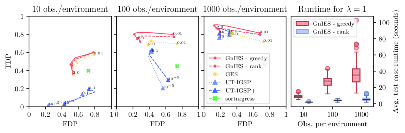
Figure 7: Recovery of the interventional Markov equivalence class for GnIES with the ranking outer procedure (red, circles, dashed) compared to the greedy approach and other algorithms. Bottom right: its runtime compared to GnIES with a greedy outer procedure. The data sets, metrics, and other algorithms are the same as in Figure 1. At the cost of a slightly reduced performance in class recovery, the ranking procedure results in a significant speed-up. The relative weight of the penalization term in the score decreases as the sample size increases, resulting in more targets being added and a higher runtime for both approaches.

The greedy outer procedure of the algorithm, as described in algorithm 2, incurs a worst-case complexity of $\mathcal{O}(p^{2}\times\text{cost of GES})$. As a faster alternative, we propose a “ranking-based” outer procedure whose complexity is instead $\mathcal{O}(p\times\text{cost of GES})$. Under this approach, we first run the inner procedure with interventions on all variables and obtain an ordering of variables based on the variance of their noise-term variance estimates. We then add (remove) targets in increasing (decreasing) order until the score does not improve. At the price of a slightly reduced performance in terms of edge recovery, the ranking procedure yields a substantial speed-up (see Figure 7 in Appendix F).

The computation of the GnIES score for interventional data is slightly more involved than for the observational equivalent used in GES, as it requires an alternating optimization routine to find the maximum likelihood estimate in (7). However, as in GES, we exploit the decomposability of the score for substantial computational savings. Since the contribution of a node to the score remains constant if its parents do not change, we can cache these “local scores” and avoid many unnecessary computations across the steps of the inner procedure of GnIES, resulting in a dramatic speed-up. Furthermore, the cache can be preserved across steps of the outer procedure, as only the local scores of nodes that are added to or removed from the intervention targets need to be recomputed. This results in further savings.

5 Experimental Results

Throughout this section, we evaluate the performance of GnIES in recovering the equivalence class of the data-generating graph across a variety of settings. As such, the estimates produced by GnIES and the baseline methods will be a set of graphs, whose closeness with the true equivalence class needs to be measured. We use the metrics introduced in Taeb et al. (2021) for this purpose, which we restate here:

Definition 3 (Metrics)

Let $\mathbb{G}^{\star}$ be the true $\mathcal{I}\text{-MEC}$ and $\hat{\mathbb{G}}$ its estimate. We define the true (false) discovery proportion respectively as

TDP : $$\max_{G^{\star}\in\mathbb{G}^{\star}}\min_{\hat{G}\in\hat{\mathbb{G}}}\big{\lvert}{\text{edges in }G^{\star}\text{ and }\hat{G}}\big{\rvert}/\big{\lvert}{\text{edges in }G^{\star}}\big{\rvert},$$

FDP : $$\max_{\hat{G}\in\hat{\mathbb{G}}}\min_{G^{\star}\in\mathbb{G}^{\star}}\big{\lvert}{\text{edges in }\hat{G}\text{ not in }G^{\star}}\big{\rvert}/\big{\lvert}{\text{edges in }\hat{G}}\big{\rvert}.$$

In the case where both the estimate and the truth are singletons, the TDP and FDP correspond to the true and false positive rates in terms of edges. The estimate and truth are equal if and only if FDP = 0 and TDP = 1.

5.1 Synthetic Data

We evaluate the performance of GnIES on simulated data and compare it to other algorithms which can be applied to the same problem setting. We consider settings where the data-generating process satisfies all model assumptions (Figure 1), and where there is a model mismatch in the nature of the interventions (Figure 2). An additional model mismatch, in the form of non-linearity and non-Gaussianity, is considered in Figure 3.

Data generation. For Figures 1 and 2 the data is sampled from 100 randomly generated linear Gaussian SCMs and intervention targets. The underlying DAGs are Erdös-Renyi graphs with $p=10$ nodes and an average degree of $2.7$. The edge weights are sampled uniformly at random from $[0.5,1]$ to bound them away from zero; the variances of the noise terms are sampled from $[1,2]$ and their mean is set to zero. We generate $10$ different data sets from each SCM consisting of samples of the same observational and interventional distributions. Each interventional distribution stems from an environment where a single variable is intervened on at random, with targets being different across environments. For Figure 1, the interventions satisfy the model assumptions, that is, they change the noise term distribution of the target by setting its variance to a value sampled uniformly at random from $[5,10]$. For Figure 2 the interventions are instead do- or hard interventions (Pearl, 2009a, Section 3.2.2), which remove the causal effect of the parents on the target and set it to a normal distribution with mean zero and variance sampled uniformly at random from $[5,10]$. For every SCM, we generate data sets with $n=10,100$, and $1000$ observations per environment.

While having access to an observational sample is not a requirement for GnIES, it is needed for a fair comparison with the other baselines. In particular, an observational environment is required by UT-IGSP; furthermore, it implies that the family of targets is conservative, an assumption required by GIES (Hauser and Bühlmann, 2012, definition 6).

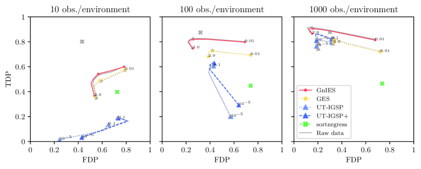
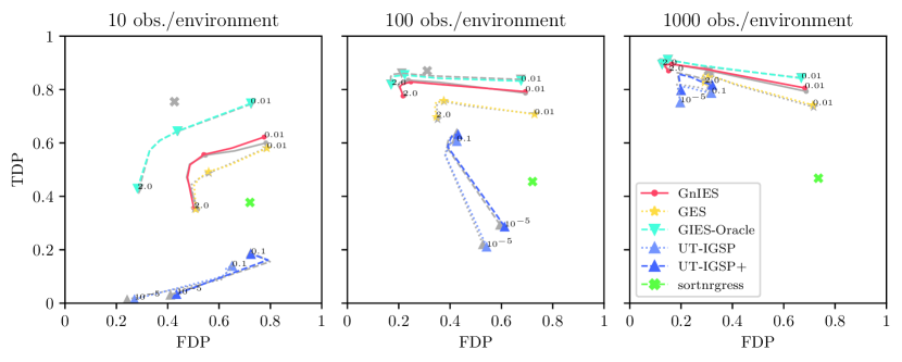
Figure 8: Performance of GnIES and the other algorithms when fed standardized (color) and raw (gray) data, for the settings with a model match (top, cf. figure 1) and a model mismatch in the form of hard interventions (bottom, cf. figure 2). The sortnregress algorithm explicitly exploits varsortability, and its performance is heavily affected when it is removed from the data via standardization. The other algorithms, including GnIES, show no significant change in performance; this can be taken as an indication that they do not rely on varsortability for inference. In both settings, the average varsortability score (Reisach et al., 2021, Section 3) is around $0.9$ for the raw data and $0.5$ for the synthetic data.

Varsortability. As shown by Reisach et al. (2021), synthetic data as generated above incurs a high degree of varsortability, that is, that marginal variance tends to increase along the causal ordering of the data-generating graph. This fact can be exploited for causal discovery, and the authors find that some recent continuous-optimization methods (Zheng et al., 2018; Ng et al., 2020) inadvertently rely on this property of synthetic data. However, this reliance means that their synthetic performance may not carry over to real-world data, where varsortability may be moderate and depends on the measurement scale; indeed, their performance broke down after standardization of the data, and when applied to the real data set from Sachs et al. (2005). To check to what extent the performance of GnIES depends on varsortability, we perform our experiments on both the standardized (Figures 1, 2) and raw (Figure 8, Appendix F) synthetic data, as advised by Reisach et al. (2021). As a sanity check, we additionally run the sortnregress algorithm proposed by Reisach et al. (2021) on the pooled data—the method shows remarkable performance in recovering the data-generating graph when there is a high varsortability in the data, and breaks down when there is not. We find that neither GnIES nor the other algorithms employed in the experiments show a significant change in performance after standardization of the data (see Figure 8 in Appendix F), an indication that they do not exploit varsortability in their inference.

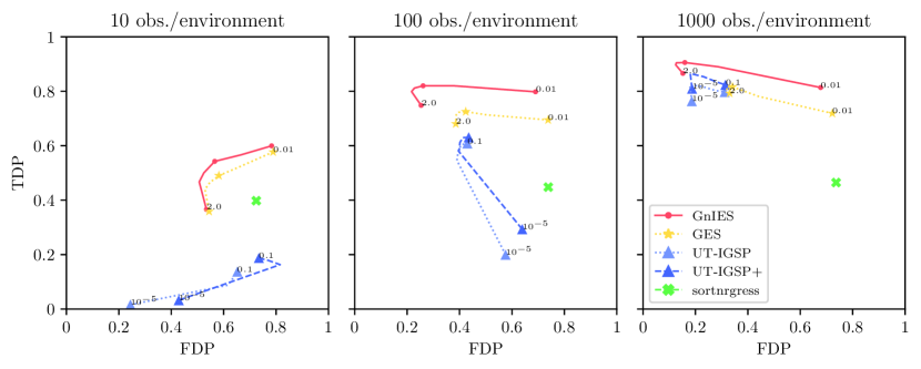
Figure 1: (correctly specified model) Recovery of the true equivalence class for different sample sizes, as measured by the metrics described in definition 3; the point $(1,0)$ corresponds to perfect recovery. The results are an average over 1000 data sets originating from 100 linear Gaussian SCMs. Because UT-IGSP returns a single DAG as estimate, we use its estimated targets and the completion algorithm of GnIES to produce an estimate of the equivalence class (displayed as UT-IGSP+). GES and sortnregress are run on the data pooled across environments. For each method, the regularization path is shown, together with the smallest and largest values of the regularizers. For GnIES and GES, the regularizer is set to $\lambda:=\lambda^{\prime}\log(N)$ where $N$ is the total number of observations and $\lambda^{\prime}\in[0.01,2]$; the additional point shown on the regularization path is for $\lambda^{\prime}=1/2$, i.e., the BIC score. For UT-IGSP, the regularizers are the levels, between $10^{-5}$ and $0.1$, of the conditional independence and invariance tests. The poor performance of sortnregress reflects the low varsortability in the data after it is standardized.

Due to its flexibility in the assumptions placed on the data-generating process, we employ UT-IGSP (Squires et al., 2020) as a baseline in all our experiments. An extension of the greedy sparse permutation algorithm (Solus et al., 2021), UT-IGSP works by measuring the conditional independencies and invariances in the data through statistical hypothesis tests, and finds the sparsest DAG and intervention targets that satisfy these constraints. The choice of tests can vary according to the setting; for the synthetic experiments of this section, we use standard partial correlation independence and invariance tests provided by the authors in their implementation of the algorithm. A drawback of the method is that it returns a single graph as estimate, when in practice there may be competing equivalent graphs, as happens in the setting that we study here. To ensure a fair comparison, we take the graph and targets estimated by UT-IGSP and compute the corresponding $\mathcal{I}$-equivalence class with the GnIES completion algorithm (see Appendix C).

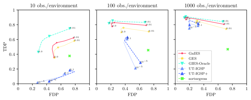
Figure 2: (model misspecification) Recovery of the interventional Markov equivalence class of the data generating model (Hauser and Bühlmann, 2012), as measured by the metrics described in definition 3; the point $(1,0)$ corresponds to perfect recovery. The results are an average over 1000 data sets originating from 100 linear Gaussian SCMs. In contrast to the other methods, GIES is run with full knowledge of the true intervention targets. GES and sortnregress are run on the data pooled across environments. Because UT-IGSP returns a single DAG as an estimate, we use its estimated targets and the completion algorithm of GIES to produce an estimate of the equivalence class (displayed as UT-IGSP+). For each method, the regularization path is shown. For GnIES, GIES and GES, the regularizer is set to $\lambda:=\lambda^{\prime}\log(N)$ where $N$ is the total number of observations and $\lambda^{\prime}\in[0.01,2]$; the additional point shown on the regularization path is for $\lambda^{\prime}=1/2$, i.e., the BIC score. For UT-IGSP, the regularizers are the levels of the conditional independence and invariance tests, taken between $10^{-5}$ and $0.1$. The poor performance of sortnregress reflects the low varsortability in the data after it is standardized.

As a baseline for the setting where the model assumptions are satisfied (Figure 1), we additionally run GES (Chickering, 2002) on the pooled data. The motivation is that this could be an initial approach employed by a practitioner to recover the class of equivalent models. Its performance suggests that this would not be entirely misguided, particularly at the smallest sample size. At this size, a possible explanation for the similar performance of GnIES and GES is that the effect of the interventions is less pronounced; due to its penalization, GnIES includes fewer intervention targets in its estimate and thus searches over classes that are often observational, essentially solving the same problem as GES. The poor performance of UT-IGSP in this sample size is not due to the diminished effect of interventions, but rather its reliance on conditional independence and invariance tests, which perform better with larger samples. Indeed, for $n=10$, in about $9\%$ of the runs the correlation matrix computed internally by UT-IGSP becomes singular, and the method fails to produce an estimate; we exclude these cases when computing the average results in the figures. As expected of the setting where all its assumptions are satisfied, GnIES performs competitively in recovering the true equivalence class and does so better than GES due to the additional identifiability.

For the setting with a model mismatch in the form of hard interventions (Figure 2), we additionally employ GIES (Hauser and Bühlmann, 2012) as a baseline, as this setting precisely satisfies the modeling assumptions of the method save for one aspect: that knowledge of the intervention targets is required. To overcome this we provide GIES with the true intervention targets, thus acting as an indicator of the ”optimum performance” we would hope to obtain if we had such knowledge. Furthermore, the equivalence class of the data-generating model is no longer the $\mathcal{I}$-equivalence class described in this paper, but rather the interventional Markov equivalence class introduced by Hauser and Bühlmann (2012). In turn, we now use the completion algorithm from GIES to compute the equivalence class estimated by UT-IGSP, from its estimated DAG and intervention targets; we note that, in practice, this would require knowledge of the model violation. Because UT-IGSP allows for a wider range of intervention types, its performance is essentially undisturbed by the change to hard interventions on the same targets. We were surprised by the good performance of GnIES in this setting, particularly when compared to that of GIES, which has access to the true intervention targets and is thus solving an easier problem. Our explanation for such behavior stems from two points. First, the $\mathcal{I}$-equivalence class is a subset of the class of equivalent models under hard interventions (c.f. proposition 3). Second, the errors in estimating the covariance matrix from a finite sample conceal the model violation and play in favor of GnIES.

5.2 Biological and Semi-synthetic Data

We now consider the protein expression data set from Sachs et al. (2005). It consists of measurements of the abundance of 11 phosphoproteins and phospholipids in human immune cells, recorded via a multiparameter flow cytometer under different experimental conditions. These conditions consist of adding reagents to the cell medium (Sachs et al., 2005, table 1), which inhibit or activate different nodes of the protein signaling network. As has been done in previous works (Squires et al., 2020; Meinshausen et al., 2016; Mooij and Heskes, 2013), we take the observations under different conditions as originating from different interventional distributions, resulting in a data set with a total of 7466 observations across nine interventional samples, each ranging from 707 to 913 observations. Furthermore, because the observations correspond to independent measurements of individual cells, we assume them to be independent and identically distributed. Since GnIES and the other baselines aim to estimate the causal structure underlying the observations, we require a ground truth to evaluate their performance. To this end, we consider the “consensus network” presented in (Sachs et al., 2005, Figure 2).

The data set is an interesting challenge because of an array of violations of the GnIES modeling assumptions. The functional relationships between variables appear to be non-linear and the distributional assumption of normality is strongly violated (see Figures 4 and 5 in Appendix E). Furthermore, the conventionally accepted structure of the protein signaling network contains cycles (see nodes PIP2, PIP3 and PLC$\gamma$ in Sachs et al., 2005, Figure 2) and, as for any measurements of real-world systems, the presence of unmeasured confounders cannot be discarded.

Figure 3: (Sachs data set) Recovery of the “consensus network” from the original Sachs data (left) and data sampled from a non-parametric SCM fitted to the original data with the consensus network structure (right). For the semi-synthetic data, the results are the average over 10 different samples from the same fitted interventional distributions. UT-IGSP corresponds to the method run with partial correlation conditional independence and invariance tests, and UT-IGSP* to the method with KCI kernel tests (Zhang et al., 2011). Because GnIES and UT-IGSP estimate interventions on all variables, their class estimates are a singleton; thus, the TDP and FDP metrics for these methods correspond to the true and false positive rates in terms of directed edge recovery. GES is run on the pooled data across environments and returns the Markov equivalence class estimated from the data. For each method, the regularization path is shown. For GnIES and GES, the regularizer is set to $\lambda:=\lambda^{\prime}\log(N)$ where $N$ is the total number of observations and $\lambda^{\prime}\in[0.01,2]$; the additional point shown on the regularization path is for $\lambda^{\prime}=1/2$, i.e., the BIC score. For UT-IGSP, the regularizers are the levels of the conditional independence and invariance tests.

Evaluation on semi-synthetic data. Another issue is that the consensus network, which is constructed from effects that appear at least once in the literature (Sachs et al., 2005, table S1), may not be a complete or accurate description of the causal relationships underlying the observations of the protein signaling network. As a safeguard, and to better understand the effect that the different model violations have on their performance, we evaluate the methods on both the original data set and semi-synthetic data sampled from a non-parametric Bayesian network, fitted to each interventional sample according to the structure of the consensus network. The sample sizes match those in the real data set. The motivation is the following: the marginal and conditional distributions of the semi-synthetic data closely resemble those of the real data and preserve the linearity and Gaussianity violations (Figures 4 and 5, Appendix E). However, it respects acyclicity, causal sufficiency (the absence of hidden confounders), and the conditional independence relations implied by the given “ground truth” graph. Thus, we can evaluate GnIES and the other baselines on two data sets of increasing difficulty, and still receive a certain degree of validation in the case of a faulty ground truth. The non-parametric SCM is fitted and sampled from using distributional random forests (Ćevid et al., 2020); the procedure is described in detail in Appendix E and can be accessed through the Python package sempler.

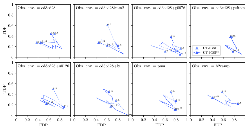
Figure 6: Performance of UT-IGSP on the Sachs data set for other choices of the observational environment. The remaining environment cd3cd28+aktinhib is displayed in Figure 3 in the main text.

As for the synthetic experiments, we run GnIES and the other methods over a range of their regularization parameters. We again run GES on the observations pooled across all samples. For UT-IGSP, we run the method with the same Gaussian tests as in the synthetic experiments and kernel-based tests (Zhang et al., 2011) provided in the implementation of the algorithm; we respectively label each approach as UT-IGSP and UT-IGSP*. Due to the nature of the experiments, it is not straightforward to select one as the observational environment for UT-IGSP. For a fair comparison, we compare the performance over every option and display the best result in Figure 3; the others can be found in Figure 6 of Appendix F.

Taking the consensus network as ground truth, there is no uniformly best performer for the real data. The performance of UT-IGSP seems to depend heavily on the level of its tests. GES performs uniformly worse than the other methods. For the semi-synthetic data and the selected regularization parameters, GnIES performs uniformly better than the other methods. The performance of UT-IGSP with Gaussian tests remains relatively unchanged and decreases with kernel tests. Several competing explanations exist for this change in performance between real and semi-synthetic data. In principle, the potential differences in the data stem from (1) the acyclicity of the data-generating model, (2) the absence of hidden confounders, or (3) a different ground truth. The interplay between these differences and the inner workings of the algorithms is poorly understood at the moment of writing. We acknowledge that without precise knowledge of the causal structure and data collection process which generated the Sachs data set, our statements about this issue are at best speculative.

6 Discussion

This paper considers a parametric approach to the problem of causal structure discovery from interventional data when the targets of interventions are unknown. For linear SCMs with additive Gaussian noise, we provide identifiability results under noise interventions and use these to develop a greedy algorithm to recover the equivalence class of the data-generating model.

When evaluated on synthetic data, the algorithm performs competitively with other algorithms built for the same setting, particularly when the available samples are small. For data arising from hard interventions, the performance matches that of the GIES algorithm (Hauser and Bühlmann, 2012) albeit lacking knowledge of the intervention targets. Thus, we believe that in situations where a practitioner may consider applying GIES, they may well apply our method and forego the need to precisely know the targets of the experiments that generated the data. To this end, we provide an easy-to-use Python implementation in the package gnies. A summary of our software contributions can be found in Appendix D.

We evaluated the algorithm on the biological data set from Sachs et al. (2005) and found its performance in recovering the “consensus network” relatively poor, but in line with other methods despite the stronger distributional assumptions. To tease apart the issues underlying this result, we developed a semi-synthetic data generation procedure, which we believe to be of general interest to the causal discovery community. The procedure allows generating semi-synthetic data sets with known causal ground truth but distributions resembling those in real data sets, providing a more realistic challenge than purely synthetic data. We detail the procedure in Appendix E and make it publicly available through the Python package sempler.

6.1 Future Work

While we have employed $\mathcal{I}$-equivalence to characterize sets of distribution equivalent Gaussian models under noise interventions, the notion is an instance of transition pair equivalence, which was introduced by Tian and Pearl (2001, theorem 2) and we detail in Section 3.1. As such, it applies beyond the Gaussian models and noise interventions we consider here. This suggests that an extension of our algorithm to more general models is justified and may be possible by appropriately adapting its score. Within the realm of Gaussian models, one could instead consider other intervention types which are still covered by the framework of Tian and Pearl (2001).

The similarity between GES and the inner procedure of GnIES suggests another line of work, based on successful extensions of GES. Under certain assumptions, constraining the maximum degree of nodes in the GES search space yielded significant improvements in sample efficiency (Chickering, 2020); a hybrid approach, using background knowledge or conditional independence tests to restrict the available operators in each step adaptively, has led to a successful scaling of GES to high-dimensional settings with thousands of variables (Nandy et al., 2018). Adapting these constraints to the $\mathcal{I}$-equivalence class may produce similar improvements for GnIES.

Acknowledgments and Disclosure of Funding

We would like to thank Jonas Peters, Jinzhou Li, and Malte Londschien for their valuable discussions and comments on the manuscript. J.L. Gamella, A. Taeb, and P. Bühlmann have received funding from the European Research Council (ERC) under the European Union’s Horizon 2020 research and innovation program (grant agreement No. 786461).

A Proofs

This section contains the proofs for all results presented in the main text of the paper. An emphasis has been placed on readability and completeness, arguably at the expense of brevity. To aid in the reading of the proofs, we summarize here the notation used and provide a graph of how the results relate to each other.

Proof map. How the presented results relate to each other. An edge $i\to j$ means that result $i$ is used to construct the proof of result $j$.

Glossary

A.1 Restated Results

We restate results from Chickering (1995, 2002) which are used in the proofs of this section. The notation is slightly adapted to fit ours.

Definition 4 (Covered edge, from Chickering, 2002)

For any DAG $G$, we say an edge $j\to i$ in $G$ is covered if

$$\textnormal{PA}_{G}(i)=\textnormal{PA}_{G}(j)\cup\{j\}.$$

Theorem 2 (Restated theorem 4 from Chickering, 2002)

Let $G$ and $H$ be any pair of DAGs such that $H$ is an independence map of $G$. Let $r$ be the number of edges in $H$ that have opposite orientation in $G$, and let $m$ be the number of edges in $H$ that do not exist in either orientation in $G$. There exists a sequence of at most $r+2m$ edge reversals and additions in $G$ with the following properties:

1. Each edge reversed is a covered edge.

2. After each reversal and addition, $G$ is a DAG and $H$ is an independence map of $G$.

3. After all reversals and additions, $G$ = $H$.

Theorem 3 (Restated theorem 2 from Chickering, 1995)

Let $G$ and $G^{\prime}$ be any pair of DAGs that are Markov equivalent and for which there are $\delta$ edges in $G$ that have opposite orientation in $G^{\prime}$. Then there exists a sequence of $\delta$ distinct edge reversals in $G$ with the following properties:

1. Each edge reversed in $G$ is covered.

2. After each edge reversal, $G$ is a DAG and is Markov equivalent to $G^{\prime}$.

3. After all reversals, $G=G^{\prime}$.

Lemma 2 (Restated lemma 1 from Chickering, 1995)

Let $G$ be any DAG model, and let $G^{\prime}$ be the result of reversing the edge $X\to Y$ in $G$. Then $G^{\prime}$ is a DAG that is Markov equivalent to $G$ if and only if $X\to Y$ is covered in $G$.

Corollary 2 (Markov equivalence and covered edge reversals)

Let $G$ and $G^{\prime}$ be two DAGs. From theorem 3 and lemma 2, it follows that they are Markov equivalent if and only if there exists a sequence of covered edge reversals that yield $G^{\prime}$ when applied to $G$.

A.2 Supporting Results from Linear Algebra

Lemma 3

Let $A\in\mathbb{R}^{p\times p}$. The following two statements are equivalent,

1. $AA^{T}$ is diagonal with positive entries, and

2. $A$ has full rank and orthogonal row vectors.

Proof  To show that $1\implies 2$, assume $AA^{T}$ is diagonal with positive entries but

1. $\text{rank}(A)<p$, or

2. $\exists i,j$ such that $i\neq j$ and $\langle A_{i:},A_{j:}\rangle\neq 0$.

If (i) is true, then $\text{rank}(A)=\text{rank}(AA^{T})<p$, which means that $\text{det}(AA^{T})=0$ and thus, since $AA^{T}$ is diagonal, $\exists i$ such that $A_{ii}=0$, which is a contradiction. If (ii) is true, then $(AA^{T})_{ij}=\langle A_{i:},A_{j:}\rangle\neq 0$, which is a contradiction.

That $2\implies 1$ is trivial, as for $i\neq j$, $(AA^{T})_{ij}=\langle A_{i:},A_{j:}\rangle=0$ by definition, and $(AA^{T})_{ii}=\langle A_{i:},A_{i:}\rangle>0$ as $A$ has full rank and $A_{i:}\neq\vec{0}$ for all $i$.  

Lemma 4

Let $A,B\in\mathbb{R}^{p\times p}$ with $B$ invertible, $\alpha\in\mathbb{R}$ and let $e_{i}\in\mathbb{R}^{p}$ be the $i^{\text{th}}$ canonical unit vector.

$$A_{i:}=\alpha B_{i:}\iff(AB^{-1})_{i:}=\alpha e_{i}^{T}.$$

Proof  ”$\implies$” $(AB^{-1})_{i:}=A_{i:}B^{-1}=\alpha B_{i:}B^{-1}=\alpha e_{i}^{T}.$
”$\impliedby$” $(AB^{-1})_{i:}=\alpha e_{i}^{T}\implies A_{i:}B^{-1}=\alpha e_{i}^{T}\implies A_{i:}=\alpha e_{i}^{T}B=\alpha B_{i:}.$  

Lemma 5 (Scaling of a matrix with orthogonal rows)

Let $M\in\mathbb{R}^{p\times p}$ be a full-rank matrix with orthogonal row vectors, such that every row has more than one non-zero entry. Let $D\in\mathbb{R}^{p\times p}$ be a diagonal matrix with positive diagonal entries for which $\exists i\in[p]$ such that $D_{ii}\neq D_{jj}$ for all $j\neq i$. Then $MD$ does not have orthogonal row vectors.

Proof  Assume that $MD$ does in fact have orthogonal row vectors, i.e., that $MDDM^{T}$ is a diagonal matrix. Denote $\tilde{M}:=MDD$, and pick $k$ such that $M_{ki}\neq 0$. We have that

$$\langle M_{k:},M_{j:}\rangle=0\text{ and }\langle\tilde{M}_{k:},M_{j:}\rangle=0\text{ for }j\neq k.$$ (8)

Since $\{M_{j:}\}_{j\neq k}$ are $p-1$ linearly independent vectors in $\mathbb{R}^{p}$, (8) implies that $\tilde{M}_{k:}$ and $M_{k:}$ belong to the same one-dimensional subspace. Thus, for some $\alpha\in\mathbb{R}$ we have that

$$\tilde{M}_{k:}= M_{k:}DD=\alpha M_{k:}$$

$$\implies M_{kl}D_{ll}^{2}=\alpha M_{kl}\text{ for all }l\in[p]$$

$$\implies D_{ll}^{2}=\alpha\text{ for all }l:M_{kl}\neq 0.$$ (9)

Note that we chose $k$ s.t. $M_{ki}\neq 0$, and because the rows of $M$ contain more than one non-zero entry, $\exists j\neq i$ such that $M_{kj}\neq 0$. Thus, (A.2) implies that $D_{ii}^{2}=\alpha=D_{jj}^{2}$. Since the diagonal entries of $D$ are positive, the above means that $D_{ii}=D_{jj}$, arriving at a contradiction with our constraints on $D$. Thus, $MD$ cannot have orthogonal row vectors, completing the proof.  

A.3 Supporting Results for the Observational Case ($\left\lvert{\mathcal{E}}\right\rvert=1$)

While the results of this subsection are known in the literature, for completeness we prove them again here for the models we consider.

Lemma 6 (I-MAPs are distribution equivalent)

Let $(B,\Omega)$ be a model with a single environment, which entails a distribution $P\sim\mathcal{N}(0,\Sigma)$ with $\Sigma:=(I-B)^{-1}\Omega(I-B)^{-T}$. Let $G$ be an independence map of $\mathcal{G}(B)$, that is, all the d-separation statements in $\mathcal{G}(B)$ hold also in $G$. Then,

$\exists$ a model $(B^{\prime},\Omega^{\prime})$ s.t. $B^{\prime}\sim G$ and $\Sigma=(I-B^{\prime})^{-1}\Omega^{\prime}(I-B^{\prime})^{-T}$.

Proof 

Case I: All edges in $\mathcal{G}(B)$ appear in $G$. Then trivially $B^{\prime}:=B$ and $\Omega^{\prime}:=\Omega$, completing the proof.

Case II: Let all the edges in $\mathcal{G}(B)$ appear in $G$, except for a single edge $j\to i$ which has been reversed to $j\leftarrow i$ in $G$. Furthermore, assume that $j\leftarrow i$ is covered in $G$. This means that

$$\textnormal{PA}_{\mathcal{G}(B)}(k)\subseteq\textnormal{PA}_{G}(k)\text{ for all }k\notin\{i,j\},$$ (10)

$$\textnormal{PA}_{\mathcal{G}(B)}(i)\setminus\{j\}\subseteq\textnormal{PA}_{G}(i),$$ (11)

$$\textnormal{PA}_{\mathcal{G}(B)}(j)\cup\{i\}\subseteq\textnormal{PA}_{G}(j),\text{ and}$$ (12)

$$\textnormal{PA}_{G}(i)\cup\{i\}=\textnormal{PA}_{G}(j).$$ (13)

We proceed to construct a connectivity matrix $B^{\prime}$ and noise term covariance $\Omega^{\prime}$ such that the result holds. First, set all but the $i^{\text{th}}$ and $j^{\text{th}}$ rows of $B^{\prime}$ to be the same as in $B$, i.e., $B^{\prime}_{k:}=B_{k:}\ \forall k\notin\{i,j\}$. We construct the remaining $i^{\text{th}}$ and $j^{\text{th}}$ rows of $B^{\prime}$ by the following rule:

$$(I-B^{\prime})_{i:}:=\beta^{i}\Omega^{-1/2}(I-B)\text{ and }(I-B^{\prime})_{j:}:=\beta^{j}\Omega^{-1/2}(I-B)$$ (14)

for some $\beta^{i},\beta^{j}\in\mathbb{R}^{p}$ such that

1. $\beta^{i}_{k}=\beta^{j}_{k}=0$ for all $k\notin\{i,j\}$,

2. $[\beta^{i}\Omega^{-1/2}(I-B)]_{i}=1$ and $[\beta^{j}\Omega^{-1/2}(I-B)]_{j}=1$.

Additionally, we impose the constraints that (iii) $\beta^{i}{\beta^{j}}^{T}=0$ and (iv) $(I-B^{\prime})_{ij}=[\beta^{i}\Omega^{-1/2}(I-B)]_{j}=0$; their purpose will become clear later. We can express all the constraints in matrix form. For the vector $\beta^{i}$ we have

$$\beta^{i}C^{i}=(0,...,0,1)\text{ where }C^{i}:=\left[\{e_{k}\}_{k\notin\{i,j\}},\Omega^{-1/2}(I-B)_{:j},\Omega^{-1/2}(I-B)_{:i}\right],$$ (15)

and for $\beta^{j}$

$$\beta^{j}C^{j}=(0,...,0,1)\text{ where }C^{j}:=\left[\{e_{k}\}_{k\notin\{i,j\}},{\beta^{i}}^{T},\Omega^{-1/2}(I-B)_{:j}\right],$$ (16)

where $e^{k}$ is the $k^{\text{th}}$ canonical unit vector. Up to a permutation of columns, $C^{i}$ is lower triangular with non-zero diagonal entries, and thus it has full rank; therefore $\beta^{i}$, as a solution to (15), exists and is unique. Plugging it into (16) yields a full rank matrix; to see this, consider that the last two columns are linearly independent from the first $p-2$ columns. The last two columns are orthogonal to each other by construction (iv). Thus, $\beta^{j}$ also exists and is unique. Now we show that the resulting $B^{\prime}$ satisfies the requirements.

$B^{\prime}$ is compatible with the graph $G$, i.e., $B^{\prime}\sim G$.

We proceed by showing that for each node $l$, $\textnormal{supp}({B^{\prime}_{l:}})\subseteq\textnormal{PA}_{G}(l)$, which implies $B^{\prime}\sim G$. Since $B^{\prime}_{k:}=B_{k:}\ \forall k\notin\{i,j\}$, by (10) it holds that $\textnormal{supp}({B^{\prime}_{k:}})=\textnormal{supp}({B_{k:}})=\textnormal{PA}_{\mathcal{G}(B)}(k)\subseteq\textnormal{PA}_{G}(k)$ for all $k\notin\{i,j\}$. Now we show that it also holds for $i$ and $j$. By (14), we have that $B^{\prime}_{i:}=\beta^{i}\Omega^{-1/2}B-\beta^{i}\Omega^{-1/2}-I_{i:},$ subject to the constraints that $B^{\prime}_{ii}=0$ (ii) and $B^{\prime}_{ij}=0$ (iv). Thus,

$$\textnormal{supp}({B^{\prime}_{i:}}) =\left(\textnormal{supp}({\beta^{i}\Omega^{-1/2}B})\cup\textnormal{supp}({\beta^{i}\Omega^{-1/2}})\cup\textnormal{supp}({I_{i:}})\right)\setminus\{i,j\}$$

by constraint (i) $$\subseteq\left(\textnormal{supp}({B_{j:}})\cup\textnormal{supp}({B_{i:}})\cup\{i,j\}\cup\{i\}\right)\setminus\{i,j\}$$

$$=\textnormal{supp}({B_{j:}})\setminus\{i,j\}\cup\textnormal{supp}({B_{i:}})\setminus\{i,j\}$$

$$=\textnormal{PA}_{\mathcal{G}(B)}(j)\setminus\{i\}\cup\textnormal{PA}_{\mathcal{G}(B)}(i)\setminus\{j\}$$

by (11, 12) $$\subseteq\textnormal{PA}_{G}(j)\setminus\{i\}\cup\textnormal{PA}_{G}(i)$$

by (13) $$=\textnormal{PA}_{G}(i)\cup\textnormal{PA}_{G}(i)$$

$$=\textnormal{PA}_{G}(i).$$

Similarly, we have that $B^{\prime}_{j:}=\beta^{j}\Omega^{-1/2}B-\beta^{j}\Omega^{-1/2}-I_{j:},$ subject to $B^{\prime}_{jj}=0$ (ii), and thus

$$\textnormal{supp}({B^{\prime}_{j:}}) =\left(\textnormal{supp}({\beta^{j}\Omega^{-1/2}B})\cup\textnormal{supp}({\beta^{j}\Omega^{-1/2}})\cup\textnormal{supp}({I_{j:}})\right)\setminus\{j\}$$

by constraint (i) $$\subseteq\left(\textnormal{supp}({B_{j:}})\cup\textnormal{supp}({B_{i:}})\cup\{i,j\}\cup\{i\}\right)\setminus\{j\}$$

$$=\left(\textnormal{supp}({B_{j:}})\cup\{i\}\cup\textnormal{supp}({B_{i:}})\right)\setminus\{j\}$$

$$=\left(\textnormal{PA}_{\mathcal{G}(B)}(j)\cup\{i\}\cup\textnormal{PA}_{\mathcal{G}(B)}(i)\right)\setminus\{j\}$$

$$=\textnormal{PA}_{\mathcal{G}(B)}(j)\cup\{i\}\cup\textnormal{PA}_{\mathcal{G}(B)}(i)\setminus\{j\}$$

by (11, 12) $$\subseteq\textnormal{PA}_{G}(j)\cup\textnormal{PA}_{G}(i)$$

by (13) $$=\textnormal{PA}_{G}(j).$$

$(B^{\prime},\Omega^{\prime})$ is a model such that $\Sigma=(I-B^{\prime})^{-1}\Omega^{\prime}(I-B^{\prime})^{-T}$.

Since $\mathcal{G}(B^{\prime})$ corresponds to a DAG, it holds that $B^{\prime}$ is lower triangular up to a permutation of rows and columns and has zero diagonal entries. Now we look at the noise term variances; let $\Omega^{\prime}:=(I-B^{\prime})(I-B)^{-1}\Omega(I-B)^{-T}(I-B^{\prime})^{T}$. By lemma 3, $\Omega^{\prime}$ is a diagonal matrix with positive entries if and only if $(I-B^{\prime})(I-B)^{-1}\Omega^{1/2}$ has full rank and orthogonal row vectors. The first condition holds as it is the product of three invertible matrices. For the orthogonality of the row vectors, note that because $B^{\prime}_{k:}=B_{k:}\ \forall k\notin\{i,j\}$, by lemma 4 we have that $[(I-B^{\prime})(I-B)^{-1}]_{k:}=e_{k}^{T}$, and thus these rows are orthogonal to each other. Furthermore, since by construction $[(I-B^{\prime})(I-B)^{-1}\Omega^{1/2}]_{ik}=\beta^{i}_{k}=0$ and $[(I-B^{\prime})(I-B)^{-1}\Omega^{1/2}]_{jk}=\beta^{j}_{k}=0\ \forall k\notin\{i,j\}$, they are also orthogonal to the $i^{\text{th}}$ and $j^{\text{th}}$ rows. These two rows are also orthogonal to one another, as by constraint (iv) we have $\beta^{i}{\beta^{j}}^{T}=0$. Thus $(B^{\prime},\Omega^{\prime})$ is a valid model for which $\Sigma=(I-B^{\prime})^{-1}\Omega^{\prime}(I-B^{\prime})^{-T}$. This completes the proof for case II.

Case III: Suppose now $G$ is any independence map of $\mathcal{G}(B)$. By theorem 2, there exists a sequence of graphs $(\mathcal{G}(B)=G_{1},G_{2},\ldots,G_{k}=G)$, where consecutive graphs differ in the reversal of a single covered edge or the addition of a single edge to $G_{i}$. We let $B^{1}:=B$, and proceeding iteratively, for each matrix $B^{i}$ and graph $G_{i+1}$ we apply the result of case I or II to obtain a new model $(B^{i+1},\Omega^{i+1})\in[(B,\Omega)]$ with $B^{i+1}\sim G_{i+1}$. At the end of this process, we can set $B^{\prime}:=B^{k}$ and $\Omega^{\prime}:=\Omega^{k}$, completing the proof.  

Corollary 3 (Markov equivalence implies distributional equivalence)

Let $(B,\Omega)$ be a model with a single environment. It follows from lemma 6 that

$$G\in\text{MEC}(\mathcal{G}(B))\implies G\in\mathbb{G}(B,\Omega).$$

Corollary 4 (Same coefficients)

From the construction of $B^{\prime}$ in the proof of lemma 6, it follows that $B_{i:}=B^{\prime}_{i:}$ for all $i$ such that $\textnormal{PA}_{\mathcal{G}(B)}(i)\subseteq\textnormal{PA}_{G}(i)$.

Lemma 7 (Under faithfulness, the true model has the minimal number of edges)

Let $(B,\Omega)$ be a model with a single environment, which entails a distribution $P\sim\mathcal{N}(0,\Sigma)$ with $\Sigma:=(I-B)^{-1}\Omega(I-B)^{-T}$. Let $\mathcal{G}(B)$ be the corresponding graph and assume that $P$ is faithful with respect to it. Then it holds that

$$\min_{G\in\mathbb{G}\left(B,\Omega\right)}\|G\|_{0}=\|\mathcal{G}(B)\|_{0}.$$

Proof  Let $\mathcal{C}(P)$ denote the set of conditional independence relationships in the distribution $P$, and let $\text{d-sep}(G)$ denote the d-separation statements entailed by some graph $G$.

Take any $G\in\mathbb{G}\left(B,\Omega\right)$. There exist $(B^{\prime},\Omega^{\prime})$ such that $B^{\prime}\sim G$ and $\Sigma=(I-B^{\prime})^{-1}\Omega^{\prime}(I-B^{\prime})^{-T}$; in other words, there exists a linear Gaussian SCM with connectivity $B^{\prime}$, noise term variances $\Omega^{\prime}$ and underlying graph $\mathcal{G}(B^{\prime})$ which entails the distribution $P$. As such, this distribution $P$ is Markov with respect to $\mathcal{G}(B^{\prime})$; because $G$ contains all edges in $\mathcal{G}(B^{\prime})$, the distribution is also Markov wrt. $G$, i.e., all d-separation relations in the graph are matched by a conditional independence relationship in $P$. Because $P$ is faithful with respect to $\mathcal{G}(B)$, it follows that $\text{d-sep}(G)\subseteq\text{d-sep}(\mathcal{G}(B))=\mathcal{C}(P)$. As such, $G$ is an independence map of $\mathcal{G}(B)$, and by theorem 2 there exists a sequence of edge reversals and additions that yield $G$ when applied to $\mathcal{G}(B)$. It follows that $G$ cannot have fewer edges than $\mathcal{G}(B)$.  

Proposition 6 (Markov and minimal-edge distributional equivalence)

Let $(B,\Omega)$ be a model as in (1) with a single environment, which entails a distribution $P\sim\mathcal{N}(0,\Sigma)$ with $\Sigma:=(I-B)^{-1}\Omega(I-B)^{-T}$. Let $\mathcal{G}(B)$ be the corresponding graph and assume that $P$ is faithful with respect to it. Then, it holds that

$$\text{MEC}(\mathcal{G}(B))=\arg\min_{G\in\mathbb{G}\left(B,\Omega\right)}\|G\|_{0},$$

where $\|G\|_{0}$ denotes the number of edges in $G$.

Proof  We show that both sets contain each other.

$\subseteq$

Let $G^{\prime}$ be a Markov equivalent graph to $\mathcal{G}(B)$. By corollary 3 there exists $(B^{\prime},\Omega^{\prime})$ in $\left[(B,\Omega)\right]$ such that $B^{\prime}\sim G^{\prime}$, and thus $G^{\prime}\in\mathbb{G}\left(B,\Omega\right)$. By lemma 7 we have that $\min_{G\in\mathbb{G}\left(B,\Omega\right)}\|G\|_{0}=\|\mathcal{G}(B)\|_{0}$; since $\mathcal{G}(B)$ and $G^{\prime}$ are Markov equivalent, they have the same number of edges, and thus $G^{\prime}\in\arg\min_{G\in\mathbb{G}\left(B,\Omega\right)}\|G\|_{0}$.

$\supseteq$

Let $\mathcal{C}(P)$ denote the set of conditional independence relationships in the distribution $P$, and let $\text{d-sep}(G)$ denote the d-separation statements entailed by some graph $G$. Take $G^{\prime}\in\arg\min_{G\in\mathbb{G}\left(B,\Omega\right)}\|G\|_{0}$; there exist $(B^{\prime},\Omega^{\prime})$ such that $B^{\prime}\sim G^{\prime}$ and $\Sigma=(I-B^{\prime})^{-1}\Omega^{\prime}(I-B^{\prime})^{-T}$; in other words, there exists a linear Gaussian SCM with connectivity $B^{\prime}$, noise term variances $\Omega^{\prime}$ and underlying graph $\mathcal{G}(B^{\prime})$ which entails the distribution $P$. As such, this distribution $P$ is Markov with respect to $\mathcal{G}(B^{\prime})$ and its independence map $G^{\prime}$. Because $P$ is faithful with respect to $\mathcal{G}(B)$, it follows that $\text{d-sep}(G^{\prime})\subseteq\text{d-sep}(\mathcal{G}(B))=\mathcal{C}(P)$, and thus $G^{\prime}$ is an independence map of $\mathcal{G}(B)$. By theorem 2 there exists a sequence $S$ of edge additions and covered-edge reversals that yield $G^{\prime}$ when applied to $\mathcal{G}(B)$. By lemma 7, $G^{\prime}$ and $\mathcal{G}(B)$ have the same number of edges; therefore, the sequence $S$ contains only covered-edge reversals and no edge additions. By corollary 2, this means that $G^{\prime}$ and $\mathcal{G}(B)$ are Markov equivalent, completing the proof.  

Lemma 8 (structure of $(I-B^{\prime})(I-B)^{-1}$ for same parents)

Consider a model $(B,\Omega)$ with a single environment and let $(B^{\prime},\Omega^{\prime})\in\left[\left(B,\Omega\right)\right]$ be an equivalent model. Let $e_{i}$ be the $i^{\text{th}}$ canonical unit vector. The following statements are equivalent:

1. $B_{i:}=B^{\prime}_{i:}$,

2. $\left[(I-B^{\prime})(I-B)^{-1}\right]_{i:}=e_{i}^{T}$, and

3. $\left[(I-B^{\prime})(I-B)^{-1}\right]_{:i}=e_{i}$.

Proof  We proceed in order.

($i\implies ii$)

Follows immediately from lemma 4.

($ii\implies iii$)

Since $(B^{\prime},\Omega^{\prime})\in\left[\left(B,\Omega\right)\right]$, it holds that $(I-B^{\prime})(I-B)^{-1}\Omega(I-B)^{-T}(I-B^{\prime})^{T}$ is a diagonal matrix with positive entries. By lemma 3, it follows that $(I-B^{\prime})(I-B)^{-1}\Omega^{1/2}$ has full rank and orthogonal row vectors. Now, since $(ii)$ is true, the $i^{\text{th}}$ row vector is $\left[(I-B^{\prime})(I-B)^{-1}\Omega^{1/2}\right]_{i:}=\Omega_{ii}^{1/2}e_{i}^{T}$, and so the remaining vectors are orthogonal to it iff they all have zeros on the $i^{\text{th}}$ coordinate, i.e., $\left[(I-B^{\prime})(I-B)^{-1}\right]_{:i}=e_{i}$.

($iii\implies i$)

Note that $(iii)$ can be rewritten as $(I-B^{\prime})(I-B)^{-1}e_{i}=e_{i}$. It follows that

$$e_{i}^{T}=e_{i}^{T}(I-B^{\prime})^{-T}(I-B)^{T}.$$ (17)

Now, since $(B^{\prime},\Omega^{\prime})\in\left[\left(B,\Omega\right)\right]$, we have that

$$(I-B^{\prime})(I-B)^{-1}\Omega(I-B)^{-T}(I-B^{\prime})^{T}=\Omega^{\prime},$$

which we can rewrite as

$$(I-B^{\prime})=\Omega^{\prime}(I-B^{\prime})^{-T}(I-B)^{T}\Omega^{-1}(I-B).$$

Multiplying on the left by $e_{i}^{T}$, and letting $\Omega^{\prime}_{ii}=\alpha$ and $\Omega^{-1}_{ii}=\beta$ we arrive at

$$e_{i}^{T}(I-B) =e_{i}^{T}\Omega^{\prime}(I-B^{\prime})^{-T}(I-B)^{T}\Omega^{-1}(I-B)$$

$$=\alpha e_{i}^{T}(I-B^{\prime})^{-T}(I-B)^{T}\Omega^{-1}(I-B)$$

$$=\alpha e_{i}^{T}\Omega^{-1}(I-B)\quad\text{(c.f. \autoref{eq:unit_column})}$$

$$=\alpha\beta e_{i}^{T}(I-B).$$

We have arrived at $(I-B)_{i:}=\alpha\beta(I-B)_{i:}$. Since both $B^{\prime}$ and $B$ have zeros on the diagonal, $(I-B)_{ii}=(I-B^{\prime})_{ii}=1=\alpha\beta(I-B)_{ii}$, which implies that $\alpha\beta=1$. Therefore, $(I-B^{\prime})_{i:}=(I-B)_{i:}$ and $B^{\prime}_{i:}=B_{i:}$.  

Lemma 9

(independence of noise terms and parents) Let $(B,\Omega)$ be a model and define the random vector $X:=(I-B)^{-1}\epsilon$ with $\epsilon\sim\mathcal{N}(0,\Omega)$. For any $i\in\{1,...,p\}$, it holds that $\epsilon_{i}\perp\!\!\!\perp X_{\textnormal{supp}}({B_{i:}})$.

Proof  We have that

$$\begin{pmatrix}\epsilon\\ X\end{pmatrix}=\begin{pmatrix}I\\ (I-B)^{-1}\end{pmatrix}\Omega^{1/2}Z\text{ with }Z=(Z_{1},...,Z_{p})\sim\mathcal{N}(0,I),$$

that is, $\epsilon$ and $X$ are jointly normal with covariance

$$\Gamma:=\begin{pmatrix}\Omega&P\\ P^{T}&\Sigma\end{pmatrix}$$

where $P:=\Omega(I-B)^{-T}$ and $\Sigma:=(I-B)^{-1}\Omega(I-B)^{-T}$. Denote $S:=\textnormal{supp}({B_{i:}})$; the joint normality implies that $\epsilon\mid X_{S}$ follows a normal distribution with mean

$$\mathbb{E}[\epsilon_{i}]+P_{i,S}\Sigma_{S,S}^{-1}(x-\mathbb{E}[X_{S}])$$ (18)

and variance

$$\Omega_{ii}-P_{i,S}\Sigma_{S,S}^{-1}P_{S,i}.$$ (19)

Now, without loss of generality, assume $B$ is lower triangular with zeros on the diagonal. It follows that

$$j<i\quad\forall i\in\{1,...,p\},\forall j\in\textnormal{supp}({B_{i:}}).$$ (20)

Since $B$ is lower triangular, so are $(I-B)$ and $(I-B)^{-1}$, and thus $P=\Omega(I-B)^{-T}$ is upper triangular. Therefore $P_{ij}=0$ for $j<i$, and together with (20), it follows that $P_{i,S}=0$. Thus, from (18, 19) we see that $\epsilon\mid X_{S}$ has mean zero and variance $\Omega_{ii}$, that is, $\epsilon_{i}\perp\!\!\!\perp X_{S}$.  

Lemma 10

(Same structure implies same coefficients) Consider a model $(B,\Omega)$ with a single environment and let $(B^{\prime},\Omega^{\prime})\in\left[\left(B,\Omega\right)\right]$ be an equivalent model. Then,

$$\textnormal{supp}({B_{i:}})=\textnormal{supp}({B^{\star}_{i:}})\iff B_{i:}=B^{\star}_{i:}.$$

Proof  The “$\impliedby$” direction is trivial. For the “$\implies$” direction, define the random vectors

$X:=(I-B)^{-1}\epsilon$ and $X^{\prime}:=(I-B^{\prime})^{-1}\epsilon^{\prime}$ with $\epsilon\sim\mathcal{N}(0,\Omega)$, $\epsilon^{\prime}\sim\mathcal{N}(0,\Omega^{\prime})$.

Let $S:=\textnormal{supp}({B_{i:}})=\textnormal{supp}({B^{\prime}_{i:}})$; we have that

$X_{i}=B_{iS}X_{S}+\epsilon_{i}$ and $X^{\prime}_{i}=B^{\prime}_{iS}X^{\prime}_{S}+\epsilon^{\prime}_{i}$.

Because $(B^{\prime},\Omega^{\prime})\in\left[\left(B,\Omega\right)\right]$, $X$ and $X^{\prime}$ follow the same distribution, and it holds that for all $x_{S}\in\mathbb{R}^{|S|}$ that

$$\mathbb{E}[X_{i}\mid X_{S}=x_{S}]=\mathbb{E}[X^{\prime}_{i}\mid X^{\prime}_{S}=x_{S}].$$

Plugging in the expression for $X_{i}$ and $X^{\prime}_{i}$ into the above, we arrive at

$$B_{iS}x_{S}+\mathbb{E}[\epsilon_{i}\mid X_{S}=x_{S}]=B^{\prime}_{iS}x_{S}+\mathbb{E}[\epsilon^{\prime}_{i}\mid X^{\prime}_{S}=x_{S}],$$

and by lemma 9, at

$$B_{iS}x_{S}+\mathbb{E}[\epsilon_{i}]=B^{\prime}_{iS}x_{S}+\mathbb{E}[\epsilon^{\prime}_{i}].$$

Since $\mathbb{E}[\epsilon_{i}]=\mathbb{E}[\epsilon^{\prime}_{i}]=0$ the above results in the condition that $(B_{iS}-B^{\prime}_{iS})x_{S}=0$ for all $x_{S}\in\mathbb{R}^{|S|}$, which is true if and only if $B_{iS}=B^{\prime}_{iS}$, completing the proof.  

A.4 Supporting Results for the Case $\left\lvert{\mathcal{E}}\right\rvert>1$

Lemma 11 (Under faithfulness, the true model has the minimum number of edges)

Consider a model $\big{(}B,\{\Omega^{e}\}_{e\in\mathcal{E}}\big{)}$ resulting in a set of distributions which are faithful with respect to its underlying graph $\mathcal{G}(B)$. Then it holds that

$$\min_{G\in\mathbb{G}\left(B,\{\Omega^{e}\}_{e\in\mathcal{E}}\right)}\|G\|_{0}=\|\mathcal{G}(B)\|.$$

Proof  Let $\mathcal{E}^{0}\subset\mathcal{E}$ be a singleton. By lemma 7 we have that $\mathcal{G}(B)$ attains the minimum number of edges in $\mathbb{G}\left(B,\{\Omega^{e}\}_{e\in\mathcal{E}^{0}}\right)$. It is trivial to see that $\mathbb{G}\left(B,\{\Omega^{e}\}_{e\in\mathcal{E}}\right)\subseteq\mathbb{G}\left(B,\{\Omega^{e}\}_{e\in\mathcal{E}^{0}}\right)$; since $\mathcal{G}(B)\in\mathbb{G}\left(B,\{\Omega^{e}\}_{e\in\mathcal{E}}\right)$, it follows that $\mathcal{G}(B)$ also attains the minimum number of edges in $\mathbb{G}\left(B,\{\Omega^{e}\}_{e\in\mathcal{E}}\right)$.  

Lemma 12 (structure of $(I-\tilde{B})(I-B)^{-1}$ for different parents)

Let $(B,\{\Omega^{e}\}_{e\in\mathcal{E}})$ be a model with a single environment, and let $(\tilde{B},\{\tilde{\Omega}^{e}\}_{e\in\mathcal{E}})\in\left[\left(B,\Omega\right)\right]$ be an equivalent model such that the diagonal entries of the matrix $M:=(I-\tilde{B})(I-B)^{-1}$ are all non-zero. Then, it holds that

$$\textnormal{supp}({B_{i:}})\neq\textnormal{supp}({\tilde{B}_{i:}})\implies\left\lvert{\textnormal{supp}({\left[(I-\tilde{B})(I-B)^{-1}\right]_{i:}})}\right\rvert>1.$$

Proof  Let $M:=(I-\tilde{B})(I-B)^{-1}$ and assume that

$\textnormal{supp}({B_{i:}})\neq\textnormal{supp}({\tilde{B}_{i:}})$ but $\left\lvert{\textnormal{supp}({M_{i:}})}\right\rvert\leq 1$.

Since $M$ has full rank it cannot be that $\left\lvert{\textnormal{supp}({M_{i:}})}\right\rvert=0$. Since the diagonal entries of $M$ cannot be zero, it must then be that $M_{i:}=[(I-\tilde{B})(I-B)^{-1}]_{i:}=\alpha e_{i}^{T}$. However, by lemma 4, this means that $(I-\tilde{B})_{i:}=\alpha(I-B)_{i:}$ and thus $\textnormal{supp}({B_{i:}})=\textnormal{supp}({\tilde{B}_{i:}})$, resulting in a contradiction.  

Lemma 13 (I-MAPs are distribution equivalent)

Consider a model $\big{(}B,\{\Omega^{e}\}_{e\in\mathcal{E}}\big{)}$ with underlying graph $\mathcal{G}(B)$. Let $\mathcal{I}=\mathbb{I}\big{(}\{\Omega^{e}\}_{e\in\mathcal{E}}\big{)}$ be the indices of variables that have received an intervention in at least one of the environments in $\mathcal{E}$. Let $G$ be an independence map of $\mathcal{G}(B)$ such that $\textnormal{PA}_{\mathcal{G}(B)}(i)\subseteq\textnormal{PA}_{G}(i)$ for all $i\in\mathcal{I}$. Then, $G\in\mathbb{G}\left(B,\{\Omega^{e}\}_{e\in\mathcal{E}}\right)$.

Proof  We want to show that there exists a model $(\tilde{B},\{\tilde{\Omega}^{e}\}_{e\in\mathcal{E}})$ such that $\tilde{B}\sim G$ and

$$(I-B)^{-1}\Omega^{e}(I-B)^{-T}=(I-\tilde{B})^{-1}\tilde{\Omega}^{e}(I-\tilde{B})^{-T}\text{ for all }e\in\mathcal{E}.$$ (21)

That is equivalent to the condition that for all $e\in\mathcal{E}$

$$\tilde{\Omega}^{e}:=(I-\tilde{B})(I-B)^{-1}\Omega^{e}(I-B)^{-T}(I-\tilde{B})^{T}$$

is a diagonal matrix with positive entries. By lemma 3, in turn this is equivalent to $(I-\tilde{B})(I-B)^{-1}(\Omega^{e})^{1/2}$ being a full-rank matrix with orthogonal row vectors, for all $e\in\mathcal{E}$. Now, let $\mathcal{E}^{0}\subset\mathcal{E}$ be a singleton and let $\Omega^{0}:=\textnormal{diag}\left(\omega_{1}^{2},...,\omega_{p}^{2}\right)$ be the noise-term variances associated to it. By lemma 6, there exists $\tilde{B}$ such that $\tilde{B}\sim G$, and $(I-\tilde{B})(I-B)^{-1}(\Omega^{0})^{1/2}$ is a full-rank matrix with orthogonal row vectors. Now, for every $e\in\mathcal{E}$, we can rewrite

$$(I-\tilde{B})(I-B)^{-1}(\Omega^{e})^{1/2}=(I-\tilde{B})(I-B)^{-1}(\Omega^{0})^{1/2}(\Omega^{0})^{-1/2}(\Omega^{e})^{1/2}.$$ (22)

If we let $\gamma_{1}^{2},...,\gamma_{p}^{2}$ be the diagonal entries of $\Omega^{e}$, we can write

$$(\Omega^{0})^{-1/2}(\Omega^{e})^{1/2}=\textnormal{diag}\left(\left\lvert{\frac{\gamma_{1}}{\omega_{1}}}\right\rvert,...,\left\lvert{\frac{\gamma_{p}}{\omega_{p}}}\right\rvert\right),$$

i.e., a diagonal matrix that constitutes a positive scaling of some of the columns of $(I-\tilde{B})(I-B)^{-1}(\Omega^{0})^{1/2}$. Note that this scaling can only occur in those columns with index in $\mathcal{I}$. Since we have assumed that $\textnormal{PA}_{\mathcal{G}(B)}(i)\subseteq\textnormal{PA}_{G}(i)$ for all $i\in\mathcal{I}$, by corollary 4 we have that $B_{i:}=\tilde{B}_{i:}$ for $i\in\mathcal{I}$, and by lemma 8, these columns have exactly one non-zero element. Scaling them leaves the matrix (22) with full rank and orthogonal row vectors, that is, for all $e\in\mathcal{E}$

$$\tilde{\Omega}^{e}:=(I-\tilde{B})(I-B)^{-1}\Omega^{e}(I-B)^{-T}(I-\tilde{B})^{T}$$

is a diagonal matrix with positive elements. Thus, (21) holds and since $\tilde{B}\sim G$ we have completed the proof.  

Lemma 14 (Targets have the same parents)

Consider a model $(B,\{\Omega^{e}\}_{e\in\mathcal{E}})$ satisfying assumptions 1 and 2, and let $\mathcal{I}:=\mathbb{I}(\{\Omega^{e}\}_{e\in\mathcal{E}})$ be the indices of variables that have received interventions in $\mathcal{E}$. Let $(\tilde{B},\{\tilde{\Omega}^{e}\}_{e\in\mathcal{E}})\in[(B,\{\Omega^{e}\}_{e\in\mathcal{E}})]$ be a distribution equivalent model. Then, $B_{i:}=\tilde{B}_{i:}$ for all $i\in\mathcal{I}$.

Proof  If $\left\lvert{\mathcal{E}}\right\rvert=1$, then $\mathcal{I}=\emptyset$ and we are done. For $\left\lvert{\mathcal{E}}\right\rvert>1$, see that because $(\tilde{B},\{\tilde{\Omega}^{e}\}_{e\in\mathcal{E}})\in[(B,\{\Omega^{e}\}_{e\in\mathcal{E}})]$ it holds that, for all $e\in\mathcal{E}$,

$$\tilde{\Omega}^{e}=(I-\tilde{B})(I-B)^{-1}\Omega^{e}(I-B)^{-T}(I-\tilde{B})^{T},$$

which implies that $M^{e}:=(I-\tilde{B})(I-B)^{-1}(\Omega^{e})^{1/2}$ is a full-rank matrix with orthogonal row vectors (lemma 3). Let $S:=\{i:B_{i:}=\tilde{B}_{i:}\}$; then, $M^{e}_{i:}=(\Omega^{e})^{1/2}e_{i}^{T}$ and $M^{e}_{:i}=(\Omega^{e})^{1/2}e_{i}$ for all $i\in S$. In other words, for any $e\in\mathcal{E}$ we have that $M^{e}$ is a block-diagonal matrix with two blocks

1. $M^{e}_{SS}$, a diagonal matrix; and

2. $M^{e}_{S^{\perp}S^{\perp}}$, where $S^{\perp}:=[p]\setminus S$.

Because of this block-diagonal form, the rows of one block are orthogonal to those of the other. Thus, $M^{e}$ has orthogonal row vectors if and only if so do both blocks. This is immediately true for the diagonal block (i). Take some $f\in\mathcal{E}:f\neq e$ and let $D:=(\Omega^{f})^{-1/2}(\Omega^{e})^{1/2}$. We can rewrite

$$M^{e}=(I-\tilde{B})(I-B)^{-1}(\Omega^{f})^{1/2}(\Omega^{f})^{-1/2}(\Omega^{e})^{1/2}=M^{f}D$$

and $M^{e}_{S^{\perp}S^{\perp}}=M^{f}_{S^{\perp}S^{\perp}}D_{S^{\perp}S^{\perp}}.$ Because $(\tilde{B},\{\tilde{\Omega}^{e}\}_{e\in\mathcal{E}})\in[(B,\{\Omega^{e}\}_{e\in\mathcal{E}})]$, by lemma 3 we have that $M^{e}$ and $M^{f}$ have full rank and orthogonal row vectors, and because of their block structure, so do $M^{e}_{S^{\perp}S^{\perp}}$ and $M^{f}_{S^{\perp}S^{\perp}}$. From assumption 2 and lemma 12, we additionally have that $M^{f}_{S^{\perp}S^{\perp}}$ has more than one non-zero element per row. Now, assume $\mathcal{I}\cap S^{\perp}\neq\emptyset$, that is, $\exists i\in\mathcal{I}$ such that $B_{i:}\neq\tilde{B}_{i:}$. Then, by intervention-heterogeneity (assumption 1), $D_{S^{\perp}S^{\perp}}$ has at least one diagonal entry different from all others. These facts allow us to apply lemma 5, by which $M^{e}_{S^{\perp}S^{\perp}}=M^{f}_{S^{\perp}S^{\perp}}D_{S^{\perp}S^{\perp}}$ does not have orthogonal rows, arriving at a contradiction. This completes the proof.  

A.5 Main Results of Section 3

Now we provide the proofs for lemma 1, proposition 1, and theorem 1.

See 1

Proof  Let $G\in\mathcal{I}\text{-MEC}(\mathcal{G}(B))$. By definition 2, this implies that $G$ is an independence map of $\mathcal{G}(B)$, and that $\textnormal{PA}_{\mathcal{G}(B)}(i)=\textnormal{PA}_{G}(i)$ for all $i\in\mathcal{I}$. Thus, by lemma 13, $G\in\mathbb{G}\left(B,\{\Omega^{e}\}_{e\in\mathcal{E}}\right)$, completing the proof.  

See 1

Proof  Let $G^{\prime}\in\mathcal{I}\text{-MEC}(\mathcal{G}(B))$. By lemma 1, $G^{\prime}\in\mathbb{G}\left(B,\{\Omega^{e}\}_{e\in\mathcal{E}}\right)$. By lemma 11 we have that $\min_{G\in\mathbb{G}\left(B,\Omega\right)}\|G\|_{0}=\|\mathcal{G}(B)\|_{0}$; since $\mathcal{G}(B)$ and $G^{\prime}$ are Markov equivalent, they have the same number of edges, and thus $G^{\prime}\in\arg\min_{G\in\mathbb{G}\left(B,\{\Omega^{e}\}_{e\in\mathcal{E}}\right)}\|G\|_{0}$, completing the proof.  

See 1

Proof  We proceed by showing both sets are contained in each other.

$\subseteq$

Follows from proposition 1.

$\supseteq$

Let $\tilde{G}\in\arg\min_{G\in\mathbb{G}\left(B,\{\Omega^{e}\}_{e\in\mathcal{E}}\right)}\|G\|_{0}$. We begin by showing that $\tilde{G}$ and $\mathcal{G}(B)$ have the same skeleton and v-structures. Let $\mathcal{E}^{0}\subset\mathcal{E}$ be a singleton and $\Omega^{0}$ be the noise-term variances associated with it. Clearly (c.f. corollary 1), $\tilde{G}\in\mathbb{G}\left(B,\Omega^{0}\right)$. Because we are under faithfulness, by lemmas 7 and 11

$$\min_{G\in\mathbb{G}\left(B,\Omega^{0}\right)}\|G\|_{0}=\|\mathcal{G}(B)\|_{0}=\min_{G\in\mathbb{G}\left(B,\{\Omega^{e}\}_{e\in\mathcal{E}}\right)}\|G\|_{0},$$

and thus $\tilde{G}\in\arg\min_{G\in\mathbb{G}\left(B,\Omega^{0}\right)}\|G\|_{0}$. By proposition 6, $\arg\min_{G\in\mathbb{G}\left(B,\Omega^{0}\right)}\|G\|_{0}=\text{MEC}(\mathcal{G}(B))$ and thus $\tilde{G}$ and $\mathcal{G}(B)$ have the same skeleton and v-structures.

If $\mathcal{E}$ is a singleton, then $\mathcal{I}=\emptyset$ and we have completed the proof. For the remaining cases, we will now show that the variables in the intervention set $\mathcal{I}$ have the same parents in $\tilde{G}$ and $\mathcal{G}(B)$. Since $\tilde{G}\in\mathbb{G}\left(B,\{\Omega^{e}\}_{e\in\mathcal{E}}\right)$, there exists a model $(\tilde{B},\{\tilde{\Omega}^{e}\}_{e\in\mathcal{E}})\in[(B,\{\Omega^{e}\}_{e\in\mathcal{E}})]$ such that $\tilde{B}\sim\tilde{G}$. First, by lemma 14, it holds that $\tilde{B}_{i:}=B_{i:}$ for all $i\in\mathcal{I}$. Second, since $\tilde{G}\in\arg\min_{G\in\mathbb{G}\left(B,\{\Omega^{e}\}_{e\in\mathcal{E}}\right)}\|G\|_{0}$, it must hold that $\mathcal{G}(\tilde{B})=\tilde{G}$ or we would have a contradiction. From these two facts, it follows that $\textnormal{PA}_{\tilde{G}}(i)=\textnormal{PA}_{\mathcal{G}(\tilde{B})}(i)=\textnormal{PA}_{\mathcal{G}(B)}(i)$ for all $i\in\mathcal{I}$, completing the proof.  

A.6 Proofs for Sections 3.1 and 3.2

Definition 5 (Augmented graph)

Given a graph $G$ over $p$ variables, and a set of targets $\mathcal{I}\subseteq[p]$, the augmented graph $G^{\mathcal{I}}$ is obtained by adding one node per intervention target to $G$, and a single edge from it to the intervened variable.

Lemma 15 (Alternative definition of $\mathcal{I}$-equivalence)

Let $G_{1}$ and $G_{2}$ be two DAGs over $p$ variables and let $\mathcal{I}\subset[p]$ be a set of intervention targets. The following statements are equivalent:

1. $G_{1}$ and $G_{2}$ are $\mathcal{I}$-equivalent, and

2. their augmented graphs $G_{1}^{\mathcal{I}}$ and $G_{2}^{\mathcal{I}}$ are Markov equivalent.

See 3

Proof  Let $\tilde{G}\in\mathcal{I}\text{-MEC}(G)$. By definition $G$ and $\tilde{G}$ are Markov equivalent, satisfying (i) in proposition 2. Since $\forall i\in\mathcal{I}:\textnormal{PA}_{G}(i)=\textnormal{PA}_{\tilde{G}}(i)$, the graphs $\tilde{G}^{(H)}$ and $G^{(H)}$ have the same skeleton for all $H\in\mathcal{H}$, satisfying (ii) and completing the proof.  

See 4

Proof  Let $\tilde{G}\in\mathcal{I}\text{-MEC}(G)$ and let $\tilde{G}^{\mathcal{Y}}$ and $G^{\mathcal{Y}}$ be the corresponding interventional DAGs. By definition 2, $\tilde{G}$ and $G$ have the same skeleton; because the edges introduced in the interventional DAGs depend only on $\mathcal{Y}$, $\tilde{G}^{\mathcal{Y}}$ and $G^{\mathcal{Y}}$ have the same additional edges and also have the same skeleton. We now show that they also have the same v-structures. Without loss of generality, suppose there exists a v-structure in $G^{\mathcal{Y}}$ which is not in $\tilde{G}^{\mathcal{Y}}$. Because the nodes $Y\in\mathcal{Y}$ do not have any parents, they can only appear in the tails of the v-structure, which can therefore be of three types:

1. $i\to k\leftarrow j$ where $i,k,j\in[p]$;

2. $Y_{1}\to k\leftarrow Y_{2}$ where $k\in[p]$ and $Y_{1},Y_{2}\in\mathcal{Y}$; or

3. $Y\to k\leftarrow j$ where $Y\in\mathcal{Y}$ and $j,k\in[p]$.

By definition 2, $\tilde{G}$ and $G$ have the same v-structures, which rules out (a). Furthermore, because the edges from nodes in $\mathcal{Y}$ to nodes in $[p]$ are the same for both $\tilde{G}^{\mathcal{Y}}$ and $G^{\mathcal{Y}}$, and they have the same skeleton, a v-structure like (b) would appear in both graphs. We now consider (c): since both graphs have the same skeleton and nodes in $\mathcal{Y}$ are always source nodes, the only option is that (c) appears instead as $Y\to k\to j$ in $\tilde{G}^{\mathcal{Y}}$. However, the edge from $Y\to k$ means that $k\in Y$, and by extension $k\in\mathcal{I}$; thus, by definition 2 $k$ would have the same parents in $\tilde{G}$ and $G$, arriving at a contradiction. Thus, we have shown that the interventional DAGs $\tilde{G}^{\mathcal{Y}}$ and $G^{\mathcal{Y}}$ have the same skeleton and v-structures, which means that $\tilde{G}\in\mathcal{Y}\text{-MEC}(G)$, completing the proof.  

A.7 Proofs of the Score Properties

We begin by stating some supporting results.

Lemma 16 ($\mathcal{I}$-equivalent graphs entail the same distributions)

Consider a set of intervention targets $\mathcal{I}\subseteq[p]$ and two graphs $G$ and $G^{\prime}$ such that $G\sim_{\mathcal{I}}G^{\prime}$. Then, for every model $(B,\{\Omega^{e}\}_{e\in\mathcal{E}})$ such that $B\sim G$ and $\mathbb{I}(\{\Omega^{e}\}_{e\in\mathcal{E}})=\mathcal{I}$, there exists a model $(\tilde{B},\{\tilde{\Omega}^{e}\}_{e\in\mathcal{E}})$ such that $\tilde{B}\sim G^{\prime}$, $\mathbb{I}(\{\tilde{\Omega}^{e}\}_{e\in\mathcal{E}})=\mathcal{I}$, and

$$(I-B)^{-1}\Omega^{e}(I-B)^{-T}=(I-\tilde{B})^{-1}\tilde{\Omega}^{e}(I-\tilde{B})^{-T}.$$

Proof  $G$ is an independence map of $\mathcal{G}(B)$ as it contains all it edges. Because $G$ and $G^{\prime}$ are $\mathcal{I}$-equivalent, $G^{\prime}$ is also an independence map of $\mathcal{G}(B)$, and since

$$\textnormal{PA}_{\mathcal{G}(B)}(i)\subseteq\textnormal{PA}_{G}(i)=\textnormal{PA}_{G^{\prime}}(i),$$ (23)

by lemma 13 there exists $(\tilde{B},\{\tilde{\Omega}^{e}\}_{e\in\mathcal{E}})$ such that $\tilde{B}\sim G^{\prime}$ and

$$(I-B)^{-1}\Omega^{e}(I-B)^{-T}=(I-\tilde{B})^{-1}\tilde{\Omega}^{e}(I-\tilde{B})^{-T}.$$ (24)

Now we will show that $\mathcal{I}=\mathbb{I}(\{\tilde{\Omega}^{e}\}_{e\in\mathcal{E}})=\mathbb{I}(\{\Omega^{e}\}_{e\in\mathcal{E}})$. As for notation, let $M:=(I-\tilde{B})(I-B)^{-1}$. Together with corollary 4, (23) implies that $B_{i:}=\tilde{B}_{i:}$ and therefore $M_{i:}=e_{i}^{T}$ and $M_{:i}=e_{i}$ for $i\in\mathcal{I}$. First we will show that $i\in\mathbb{I}(\Omega^{e}\}_{e\in\mathcal{E}}\implies i\in\mathbb{I}(\{\tilde{\Omega}^{e}\}_{e\in\mathcal{E}})$. Note that (c.f. equation 5)

$$i\in\mathcal{I}=\mathbb{I}(\Omega^{e}\}_{e\in\mathcal{E}})\iff\exists e,f\in\mathcal{E}:[\Omega^{e}(\Omega^{f})^{-1}]_{ii}\neq 1.$$ (25)

We can rewrite (24) as $\tilde{\Omega}^{e}=M\Omega^{e}M^{T},$ and thus $\tilde{\Omega}^{e}(\tilde{\Omega}^{f})^{-1}=M\Omega^{e}(\Omega^{f})^{-1}M^{-1}$. For $i\in\mathcal{I}$ we have that

$$[\tilde{\Omega}^{e}(\tilde{\Omega}^{f})^{-1}]_{ii} =M_{i:}\Omega^{e}(\Omega^{f})^{-1}M^{-1}_{:i}$$

$$=e_{i}^{T}\Omega^{e}(\Omega^{f})^{-1}M^{-1}_{:i}\quad\text{(}M_{i:}=e_{i}^{T},\text{ see above)}$$

$$=[\Omega^{e}(\Omega^{f})^{-1}]_{ii}e_{i}^{T}M^{-1}_{:i}\quad\text{(}\Omega^{e},\Omega^{f}\text{ are diagonal)}$$

$$=[\Omega^{e}(\Omega^{f})^{-1}]_{ii}M_{i:}M^{-1}_{:i}$$

$$=[\Omega^{e}(\Omega^{f})^{-1}]_{ii}\neq 1,$$

and thus by (25) $i\in\mathbb{I}(\{\tilde{\Omega}^{e}\}_{e\in\mathcal{E}})$. Now we will show that $j\notin\mathbb{I}(\Omega^{e}\}_{e\in\mathcal{E}}\implies j\notin\mathbb{I}(\{\tilde{\Omega}^{e}\}_{e\in\mathcal{E}})$. Note that

$$j\notin\mathcal{I}=\mathbb{I}(\Omega^{e}\}_{e\in\mathcal{E}})\iff[\Omega^{e}-\Omega^{f}]_{jj}=0\;\forall e,f\in\mathcal{E}.$$ (26)

Now, pick any $e,f\in\mathcal{E}$ and see from (24) that $\tilde{\Omega}^{e}-\tilde{\Omega}^{f}=M(\Omega^{e}-\Omega^{f})M^{T}$. Because $M_{:i}=e_{i}$ for $i\in\mathcal{I}$, it follows that $M_{ji}=0$ for $j\notin\mathcal{I}$. Thus, we have that

$$[\tilde{\Omega}^{e}-\tilde{\Omega}^{f}]_{jj}=M_{j:}(\Omega^{e}-\Omega^{f})M^{T}_{:j}=\sum_{i\in\mathcal{I}}M_{ij}[\Omega^{e}-\Omega^{f}]_{ii}+\sum_{k\notin\mathcal{I}}M_{kj}[\Omega^{e}-\Omega^{f}]_{kk}=0,$$

as by (26) $[\Omega^{e}-\Omega^{f}]_{kk}=0$ in the second sum. Because we picked $e,f$ arbitrarily, this means that $[\tilde{\Omega}^{e}-\tilde{\Omega}^{f}]_{jj}=0$ for all $e,f\in\mathcal{E}$ and thus, by the same argument as in (26), $j\notin\mathbb{I}(\{\tilde{\Omega}^{e}\}_{e\in\mathcal{E}})$. Together with the previous results, this shows that $\mathbb{I}(\{\tilde{\Omega}^{e}\}_{e\in\mathcal{E}})=\mathbb{I}(\{\Omega^{e}\}_{e\in\mathcal{E}})=\mathcal{I}$, completing the proof.  

See 5

Proof of score equivalence

Consider a set $\mathcal{I}\subseteq[p]$ of intervention targets and two graphs $G$ and $G^{\prime}$ such that $G\sim_{\mathcal{I}}G^{\prime}$. We want to show that they attain the same score over any sample, that is $S(G,\mathcal{I})=S(G^{\prime},\mathcal{I})$. Note that we can rewrite

$$\log P\left(\boldsymbol{X}^{e};{B},\{{\Omega}^{e}\}_{e\in\mathcal{E}}\right)=-n_{e}\ln\mathrm{det}({K}^{e})-n_{e}\mathrm{tr}({K}^{e}\hat{\Sigma}^{e}),$$ (27)

where $\hat{\Sigma}^{e}$ is the sample covariance for environment $e$, and $K^{e}:=[(I-B)^{-1}\Omega^{e}(I-B)^{-T}]^{-1}$ is the inverse of the covariance matrix entailed by the model for environment $e$. Thus, we can rewrite the score (7) as

$$S(G,\mathcal{I})=\max_{\begin{subarray}{c}B\sim G\\ \text{diagonal }\{\Omega^{e}\}_{e\in\mathcal{E}}\\ \text{s.t. }\mathbb{I}(\{\Omega^{e}\}_{e\in\mathcal{E}})=\mathcal{I}\end{subarray}}\quad\sum_{e\in\mathcal{E}}n_{e}\ln\mathrm{det}({K}^{e})-n_{e}\mathrm{tr}({K}^{e}\hat{\Sigma}^{e})-\lambda\text{DoF}(G,\mathcal{I}).$$ (28)

Now, let $(B,\{\Omega^{e}\}_{e\in\mathcal{E}})$ be the model parameters which maximize the score for $G$. By lemma 16, there exists $(\tilde{B},\{\tilde{\Omega}^{e}\}_{e\in\mathcal{E}})$ for which $\tilde{B}\sim G^{\prime}$ and

$$(I-B)^{-1}\Omega^{e}(I-B)^{-T}=(K^{e})^{-1}=(I-\tilde{B})^{-1}\Omega^{e}(I-\tilde{B})^{-T}.$$

Furthermore, because $G$ and $G^{\prime}$ have the same number of edges, $\text{DoF}(G,\mathcal{I})=\text{DoF}(G^{\prime},\mathcal{I})$ and $S(G,\mathcal{I})\leq S(G^{\prime},\mathcal{I})$. If we apply the same reasoning to $G^{\prime}$ and its maximizing parameters, we arrive at $S(G,\mathcal{I})\geq S(G^{\prime},\mathcal{I})$. It must hold that $S(G,\mathcal{I})=S(G^{\prime},\mathcal{I})$, completing the proof.

Proof of decomposability

Note that if $B\in\mathbb{R}^{p\times p}$ has zeros on the diagonal and is lower triangular up to a permutation of rows and columns, then $(I-B)$ can be expressed as $PLP$ for some permutation matrix $P$ and some lower-triangular matrix $L$ with ones on the diagonal. Thus, $\mathrm{det}((I-B)^{T})=\mathrm{det}((I-B))=1$, and we can rewrite the logarithm term in (27) as

$$\ln\mathrm{det}({K}^{e})=\ln[\mathrm{det}((I-B)^{T})\mathrm{det}((\Omega^{e})^{-1})\mathrm{det}(I-B)]=\ln(\prod_{i\in[p]}1/\Omega^{e}_{ii})=-\sum_{i\in[p]}\ln\Omega^{e}_{ii}$$

For the trace term, we have that

$$\mathrm{tr}({K}^{e}\hat{\Sigma}^{e})=\mathrm{tr}((I-B)^{T}(\Omega^{e})^{-1}(I-B)\hat{\Sigma}^{e})=\mathrm{tr}((\Omega^{e})^{-1}(I-B)\hat{\Sigma}^{e}(I-B)^{T}),$$

where the last equality stems from the invariance of the trace to cyclic permutations. By rewriting the trace of products as the sum of entry-wise products, we have that

$$\mathrm{tr}({K}^{e}\hat{\Sigma}^{e})=\sum_{i\in[p]}\sum_{j\in[p]}1/\Omega^{e}_{ij}[(I-B)\hat{\Sigma}^{e}(I-B)^{T})]_{ij}=\sum_{i\in[p]}1/\Omega^{e}_{ii}[(I-B)\hat{\Sigma}^{e}(I-B)^{T})]_{ii},$$

and thus $\mathrm{tr}({K}^{e}\hat{\Sigma}^{e})=\sum_{i\in[p]}1/\Omega^{e}_{ii}(I-B)_{i:}\hat{\Sigma}^{e}(I-B)^{T})_{:i}$. Together with the new expression for the logarithm term, we can rewrite the score (A.7) as

$$S(G,\mathcal{I}) =\sum_{i\in[p]}\max_{\begin{subarray}{c}B_{i:},\{\Omega_{ii}^{e}\}_{e\in\mathcal{E}}\\ \text{s.t.}\\ \textnormal{supp}({B_{i:}})\subseteq\textnormal{PA}_{G}(i)\\ \Omega_{ii}>0\end{subarray}}\sum_{e\in\mathcal{E}}-n_{e}\left[\ln\Omega^{e}_{ii}+1/\Omega^{e}_{ii}(I-B)_{i:}\hat{\Sigma}^{e}(I-B)^{T})_{:i}\right]-\lambda\text{DoF}(i,G,\mathcal{I}),$$

where $\text{DoF}(i,G,\mathcal{I})=\left\lvert{\textnormal{PA}_{G}(i)}\right\rvert+\mathrm{max}(\left\lvert{\mathcal{E}}\right\rvert\boldsymbol{1}_{\{i\in\mathcal{I}\}},1)$ are the number of parameters estimated for variable $i$. In other words, the score decouples into a sum of terms depending only on each variable and its parents, which completes the proof.

Proof of consistency

Throughout, we consider $p$ fixed and $n_{e}\to\infty$ for every $e\in\mathcal{E}$.
For every $G\in\mathcal{I}^{\star}\text{-MEC}(G^{\star})$, let $(B,\{\Omega^{e}\}_{e\in\mathcal{E}})$ be the unique connectivity matrix and noise variances that specify the population covariance matrices $\{\Sigma^{e}\}_{e\in\mathcal{E}}$. In our analysis, the parameter space $(B,\{\Omega^{e}\}_{e\in\mathcal{E}}$ is assumed to be compact. For notational ease, we denote the constraint set for the parameters $(B,\{\Omega^{e}\}_{e\in\mathcal{E}})$ as $\Theta$. Assuming such a compactness constraint enables uniform convergence of M-estimators (van de Geer, 2000). As an example of a compactness constraint, let $\tau_{1},\tau_{2},\tau_{3}>0$ be scalars where for every such $(B,\{\Omega^{e}\}_{e\in\mathcal{E}})$, $\|(I-B)\|_{F}\leq\tau_{1}$, $\min_{i,e}|\Omega^{e}_{ii}|\geq\tau_{2}$, and $\max_{i,e}|\Omega^{e}_{ii}|\leq\tau_{3}$. Then, the space of connectivity matrices and noise variances has the additional constraints $\|(I-B)\|_{F}\leq\tau_{1}$, $\min_{i,e}|\Omega^{e}_{ii}|\geq\tau_{2}$ and $\max_{i,e}|\Omega^{e}_{ii}|\leq\tau_{3}$ in the score function. We denote the score of a DAG $G$ and intervention set $\mathcal{I}$ when constrained to the compact parameter space $\Theta$ as $S(G,\mathcal{I})$.

For any $G$ and intervention set $\mathcal{I}$, we let $S^{\star}(G,\mathcal{I})$ be the score in population, namely:

$$S^{\star}(G,\mathcal{I})=\max_{(B,\{\Omega^{e}\}_{e\in\mathcal{E}})\in\Theta}\sum_{e\in\mathcal{E}}\pi^{e,\star}\left[-\ln\mathrm{det}(\Omega^{e})-\mathrm{tr}((I-B)^{T}(\Omega^{e})^{-1}(I-B)\Sigma^{e,\star})\right],$$

where $\Sigma^{e,\star}$ represents the true covariance in environment $e$ and $\pi^{e,\star}={\lim_{\mbox{all}\ n_{e}\to\infty}}\frac{n^{e}}{\sum_{e\in\mathcal{E}}n^{e}}$. Notice that the minimizers $\operatorname*{arg\,min}_{G,\mathcal{I}}S^{\star}(G,\mathcal{I})$ are the distributionally equivalent models to the population model $(B^{\star},\{\Omega^{e,\star}\}_{e\in\mathcal{E}})$.

First, we show that for every $G$ and intervention set $\mathcal{I}$, the score function $S(G,I)\overset{p}{\to}S^{\star}(G,I)$ as $n_{e}\to\infty$ for every $e\in\mathcal{E}$. This follows by the compactness of the parameter space leading to uniform convergence of M-estimators, and that $\lambda\to 0$ (van de Geer, 2000). For more details, note that:

$$S(G,\mathcal{I})+\lambda\text{DoF}(G,\mathcal{I})=\max_{(B,\{\Omega^{e}\}_{e\in\mathcal{E}})\in\Theta} \sum_{e\in\mathcal{E}}\pi^{e,\star}\left[-\ln\mathrm{det}(\Omega^{e})-\mathrm{tr}((I-B)^{T}(\Omega^{e})^{-1}(I-B)\Sigma^{e,\star})\right]$$

$$-\mathrm{tr}((I-B)^{T}(\Omega^{e})^{-1}(I-B)(\hat{\pi}^{e}\hat{\Sigma}^{e}-{\pi}^{e,\star}\Sigma^{e,\star}))$$

$$-(\hat{\pi}^{e}-\pi^{e,\star})\ln\mathrm{det}(\Omega^{e})$$

where $\hat{\pi}^{e}=\frac{n^{e}}{\sum_{e\in\mathcal{E}}n^{e}}$. From there, we have

$$S(G,\mathcal{I}) \geq S^{\star}(G,\mathcal{I})-\max_{(B,\{\Omega^{e}\}_{e\in\mathcal{E}})\in\Theta}\sum_{e\in\mathcal{E}}\mathrm{tr}\left((I-B)^{T}(\Omega^{e})^{-1}(I-B)(\hat{\pi}^{e}\hat{\Sigma}^{e}-{\pi}^{e,\star}\Sigma^{e,\star}))\right)$$

$$-\max_{(B,\{\Omega^{e}\}_{e\in\mathcal{E}})\in\Theta}\sum_{e\in\mathcal{E}}(\hat{\pi}^{e}-\pi^{e,\star})\ln\mathrm{det}(\Omega^{e})-\lambda~{}\text{DoF}(G,\mathcal{I})$$

$$S(G,\mathcal{I}) \leq S^{\star}(G,\mathcal{I})+\max_{(B,\{\Omega^{e}\}_{e\in\mathcal{E}})\in\Theta}\sum_{e\in\mathcal{E}}\mathrm{tr}\left((I-B)^{T}(\Omega^{e})^{-1}(I-B)(\hat{\pi}^{e}\hat{\Sigma}^{e}-{\pi}^{e,\star}\Sigma^{e,\star})\right)$$

$$+\max_{(B,\{\Omega^{e}\}_{e\in\mathcal{E}})\in\Theta}\sum_{e\in\mathcal{E}}(\hat{\pi}^{e}-\pi^{e,\star})\ln\mathrm{det}(\Omega^{e}).$$

By the compactness constraint,

$$\max_{(B,\{\Omega^{e}\}_{e\in\mathcal{E}})\in\Theta}\sum_{e\in\mathcal{E}}\mathrm{tr}\left((I-B)^{T}(\Omega^{e})^{-1}(I-B)(\hat{\pi}^{e}\hat{\Sigma}^{e}-{\pi}^{e,\star}\Sigma^{e,\star})\right)\to 0$$

$$\max_{(B,\{\Omega^{e}\}_{e\in\mathcal{E}})\in\Theta}\sum_{e\in\mathcal{E}}(\hat{\pi}^{e}-\pi^{e,\star})\ln\mathrm{det}(\Omega^{e})\to 0$$

as $n^{e}\to\infty$. Furthermore, since $\lambda\to 0$ as $n^{e}\to\infty$ for every $e\in\mathcal{E}$, and $\text{DoF}(G,\mathcal{I})$ is bounded, we have that $\lambda\text{DoF}(G,\mathcal{I})\to 0$. We can thus conclude $S(G,\mathcal{I})\to S^{\star}(G,\mathcal{I})$ in the infinite data limit for every environment.

Suppose the regularization parameter $\lambda\to 0$ and is chosen such that for every $e\in\mathcal{E}$, it is above fluctuations due to sampling error:

$$\lambda \gg\left|\max_{(B,\{\Omega^{e}\}_{e\in\mathcal{E}})\in\Theta}\sum_{e\in\mathcal{E}}\mathrm{tr}\left((I-B)^{T}(\Omega^{e})^{-1}(I-B)(\pi^{e,\star}\Sigma^{e,\star}-\hat{\pi}^{e}\hat{\Sigma}^{e})\right)\right|$$

$$+\left|\max_{(B,\{\Omega^{e}\}_{e\in\mathcal{E}})\in\Theta}\sum_{e\in\mathcal{E}}(\hat{\pi}^{e}-\pi^{e,\star})\ln\mathrm{det}(\Omega^{e})\right|$$

With this choice of the regularization, it follows that among any distributionally equivalent models $(G,\mathcal{I})$ and $(G^{\prime},\mathcal{I}^{\prime})$, if $\text{DoF}(G,\mathcal{I})<\text{DoF}(G,\mathcal{I})$, then, there exists $N$ such that for any $n^{e}\geq N$, $S(G,\mathcal{I})>S(G^{\prime},\mathcal{I}^{\prime})$. This allows us to conclude that:

$$\mathbb{P}\left(\operatorname*{arg\,min}S(G,\mathcal{I})=\operatorname*{arg\,min}\text{DoF}(G,\mathcal{I})\text{ subject-to }G,\mathcal{I}\in\operatorname*{arg\,min}S^{\star}(G,\mathcal{I})\right)\to 1,$$

as $n^{e}\to\infty$ for every $e\in\mathcal{E}$. In other words, in the infinite data limit, the minimizers of $\operatorname*{arg\,min}_{G,\mathcal{I}}S(G,\mathcal{I})$ are given by:

$$\arg\min_{G,\mathcal{I}} ~{}~{}\text{DoF}(G,\mathcal{I})$$ (29)

subject-to $$~{}~{}B\sim G,\mathcal{I}=\mathbb{I}(\{\Omega^{e}\}_{e\in\mathcal{E}}),\text{ and}$$

$$~{}~{}\Sigma_{e}^{\star}=(I-B)^{-1}\Omega^{e}(I-B)^{-T}~{}~{}\text{ for every }e\in\mathcal{E}.$$

Our remaining goal is to show that $\mathcal{I}^{\star}\text{-MEC}(\mathcal{G}(B^{\star}))$ is the set of minimizers in (29). By definition, $\Sigma_{e}^{\star}=(I-B^{\star})^{-1}{\Omega^{e,\star}}(I-B^{\star})^{-T}$ for every $e\in\mathcal{E}$. Since the model $(B^{\star},\{\Omega^{e,\star}\}_{e\in\mathcal{E}})$ satisfies assumptions 1 and 2, we appeal to lemma 14 to conclude that a feasible $B$ in (29) satisfies $B_{i,:}=B^{\star}_{i,:}$ for all $i\in\mathcal{I}^{\star}$. Since $(I-B^{\star})^{-1}{\Omega^{e,\star}}(I-B^{\star})^{-T}=(I-B)^{-1}\Omega^{e}(I-B)^{-T}$, the previous conclusion implies that $\Omega^{e,\star}_{ii}=\Omega^{e}_{ii}$ for all $i\in\mathcal{I}^{\star}$ and feasible $\{\Omega^{e}\}_{e\in\mathcal{E}}$. Thus, any feasible $\mathcal{I}$ satisfies $\mathcal{I}\supseteq\mathcal{I}^{\star}$. Furthermore, from theorem 1 we know that:

$$\mathcal{I}^{\star}\text{-MEC}(G^{\star})=\arg\min_{G,I} ~{}~{}\text{DoF}(G)$$ (30)

subject-to $$~{}~{}B\text{ compatible with }G$$

$$~{}~{}\Sigma_{e}^{\star}=(I-B)^{-1}\Omega^{e}(I-B)^{-T}~{}~{}\text{ for every }e\in\mathcal{E}$$

Notice that $\text{DoF}(G,\mathcal{I})=\text{DoF}(G)+\text{DoF}(\mathcal{I})$. Combining this the relation in (30) and the fact that any feasible $\mathcal{I}$ in (29) satisfies $\mathcal{I}\supseteq\mathcal{I}^{\star}$, we arrive at the desired result.

B Discussion of Assumption 2

We restate assumption 2 here for completeness.

See 2 A violation of assumption 2 would imply that, given some conditioning set, the conditional variance of a variable, is not a function of the variance of its noise term. We formalize and prove this statement in lemma 17 below.

Lemma 17 (Violation of assumption 2)

Let $(B,\Omega)$ be a model and $X:=(I-B)^{-1}\epsilon$ with $\epsilon\sim\mathcal{N}(0,\Omega)$ the normal random vector it entails. If there exists an equivalent model $(B^{\prime},\Omega^{\prime})\in[(B,\Omega)]$ such that $[(I-B^{\prime})(I-B)^{-1}]_{ii}=0$, then there exists $S\subseteq[p]\setminus\{i\}$ for which the variance of $X_{i}$ given $X_{S}$ is not a function of the variance of its noise-term $\epsilon_{i}$.

Proof  Because $(B^{\prime},\Omega^{\prime})\in[(B,\Omega)]$, we have that

$$(I-B)^{-1}\Omega(I-B)^{-T}=(I-B^{\prime})^{-1}\Omega^{\prime}(I-B^{\prime})^{-T}.$$ (31)

Now, let $M:=(I-B^{\prime})(I-B)^{-1}$ and assume $M_{ii}=0$ for some $i\in[p]$. It must hold that $\textnormal{supp}({B_{i:}})\neq\textnormal{supp}({B^{\prime}_{i:}})$, or by lemmas 10 and 8 we would have $[(I-B)(I-B^{\prime})]_{ii}=1$. Define $X^{\prime}:=(I-B^{\prime})^{-1}\epsilon^{\prime}$ with $\epsilon^{\prime}\sim\mathcal{N}(0,\Omega^{\prime})$ and let $S:=\textnormal{supp}({B^{\prime}_{i:}})$. Because the models are equivalent, the random vectors $X$ and $X^{\prime}$ follow the same distribution. Thus, for all $x_{S}\in\mathbb{R}^{\left\lvert{S}\right\rvert}$

$$\textnormal{Var}(X_{i}\mid X_{s}=x_{S}) =\textnormal{Var}(X^{\prime}_{i}\mid X^{\prime}_{s}=x_{S})$$

by (1) $$=\textnormal{Var}\Big{(}{\sum_{j\in S}B^{\prime}_{ij}X^{\prime}_{j}+\epsilon^{\prime}_{i}\mid X^{\prime}_{s}=x_{S}}\Big{)}$$

$$=\textnormal{Var}\left(B^{\prime}_{iS}x_{S}+\epsilon^{\prime}_{i}\mid X^{\prime}_{s}=x_{S}\right)$$

$$=\textnormal{Var}\left(\epsilon^{\prime}_{i}\mid X^{\prime}_{s}=x_{S}\right)$$

by lemma 9 $$=\textnormal{Var}(\epsilon^{\prime}_{i})=\Omega^{\prime}_{ii}$$

by (31) $$=\sum_{j\in[p]}M^{2}_{ij}\Omega_{jj}$$

because $$M_{ii}=0 =\sum_{j\neq i}M^{2}_{ij}\Omega_{jj}.$$

In other words, the conditional variance of $X_{i}$ given $X_{S}$ is not a function of its noise-term variance $\Omega_{ii}$.  
As additional empirical support for the claim that assumption 2 is a direct consequence of faithfulness and our modeling assumptions, we check that the assumption indeed holds for all random models generated in the synthetic experiments of Section 5.

C GnIES Completion Algorithm

Below we detail the completion algorithm used at the end of each step of the inner procedure from GnIES. The algorithm is also employed in the experiments to compute an estimate of the equivalence class from the graph and intervention targets returned by UT-IGSP.

Algorithm 3 Completion algorithm for the inner procedure of GnIES

1:  Input: PDAG $P$, intervention set $\mathcal{I}$.
Precondition: The PDAG $P$ has no undirected in- or out-going edges from the nodes in $\mathcal{I}$; this is guaranteed during the inner procedure of GnIES.

2:  Obtain the CPDAG $C$ by completing $P$ using the GES completion algorithm (Chickering, 2002, Appendix C)

3:  Orient edges: For every node in $\mathcal{I}$, orient all in- and out-going edges to match the orientation in the original PDAG $P$

4:  Apply the Meek rules (Meek, 1995) iteratively to $C$ until no more edges can be oriented.

5:  Output: The I-CPDAG $C$ representing the $\mathcal{I}\text{-MEC}$.

D Software Contributions

The code, data sets and instructions to reproduce the experiments and figures in the manuscript can be found in the repository github.com/juangamella/gnies-paper. The Python implementation of the GnIES algorithm is available through the gnies package (see details below). During our work on this paper, we developed additional software which we make available through the Python packages listed below. The packages are well documented, actively maintained, and available through the python package index, that is, they can easily be installed with Python’s package manager by typing pip install <package_name> into a suitable terminal. More details and installation instructions can be found in their respective repositories, listed below.

Package	Description	Details and documentation
gnies	The GnIES algorithm.	github.com/juangamella/gnies
ges	A pure Python implementation of the GES algorithm (Chickering, 2002).	github.com/juangamella/ges
gies	A pure Python implementation of the GIES algorithm from Hauser and Bühlmann (2012).	github.com/juangamella/gies
sempler	Used to generate the synthetic and semi-synthetic data used in the experiments.	github.com/juangamella/sempler

E Semi-synthetic Data Generation Procedure

In this section we summarize the procedure used to generate the semi-synthetic data set from Section 5, generated by combining the biological data set and consensus graph given in Sachs et al. (2005). The procedure is general in that it can be used with any other data set and graph; an implementation is provided in the python package sempler.

As input, we are given a directed acyclic graph $\mathcal{G}$ over $p$ variables and a data set consisting of their observations under different environments. The procedure then fits a non-parametric Bayesian network which approximates the conditional distributions entailed by the factorization of the graph $\mathcal{G}$ via distributional random forests (Ćevid et al., 2020). Once fitted, we can sample from this collection of forests to produce a new, semi-synthetic data set that respects the conditional independence relationships entailed by $\mathcal{G}$, while its marginal and conditional distributions closely match those of the original data set (figures 4 and 5).

The procedure is motivated by a fundamental concept from graphical models. We say a distribution $P$ satisfies the global Markov property with respect to a DAG $\mathcal{G}$ if and only if it factorizes according to its parental relations (Pearl, 1988), that is, if

$$P(X_{1},...,X_{p})=\prod_{j\in[p]}P(X_{j}\mid X_{\textnormal{PA}_{\mathcal{G}}(j)}).$$

Thus, we can model the joint data-generating distribution by independently modeling the conditional distribution of each variable given its parents in $\mathcal{G}$. We take this approach and model the collection of data-generating distributions $\{P^{e}\}_{e\in\mathcal{E}}$ as follows: for each environment $e\in\mathcal{E}$ and each node $j\in[p]$, we estimate $\hat{P}^{e}_{X_{j}\mid X_{\textnormal{PA}_{\mathcal{G}}(j)}=x}$ by fitting a distributional random forest (Ćevid et al., 2020). Note that while the distributions $\{P^{e}\}_{e\in\mathcal{E}}$ of the data may not satisfy the Markov condition with respect to $\mathcal{G}$, the estimated distributions $\{\hat{P}^{e}\}_{e\in\mathcal{E}}$ do.

We can now generate new data by sampling from the estimated conditional distributions, following the causal ordering of the DAG $\mathcal{G}$. We proceed as follows:

1. First, we obtain the causal ordering $O_{\mathcal{G}}$ of $\mathcal{G}$.

2. Then, for every environment $e\in\mathcal{E}$ and the next (or first) node in $O_{\mathcal{G}}$:

   1. if $j$ is a source node, we generate a sample $\left\{\hat{x}^{e}_{j}(i)\right\}_{i=1,...,n_{e}}$ via bootstrapping, where $n_{e}$ is the number of observations from environment $e$ in the original data set.

   2. If $j$ is not a source node, for every new observation $i=1,...,n_{e}$ we sample

      $$\hat{X}^{e}_{j}(i)\sim\hat{P}^{e}_{X_{j}\mid X_{\textnormal{PA}_{\mathcal{G}}(j)}=\hat{x}^{e}_{\textnormal{PA}_{\mathcal{G}}(j)}(i)}$$

      using the technique provided by Ćevid et al. (2020), where $\hat{x}^{e}_{\textnormal{PA}_{\mathcal{G}}(j)}(i)$ is the previously sampled observation for the parents of $j$.

3. We collect all the samples, resulting in a new semi-synthetic data set.

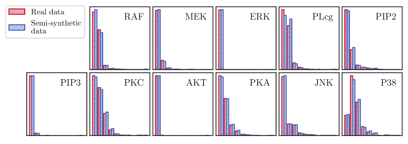
Figure 4: Histograms of the observations of each variable measured in the Sachs data set, for the real data (red, dots) and the semi-synthetic data (blue, stripes) sampled from the network fitted to the data set using distributional random forests (Ćevid et al., 2020) following the consensus network. The marginals of the semi-synthetic data closely resemble those of the real data, and both show strong indications of non-normality.

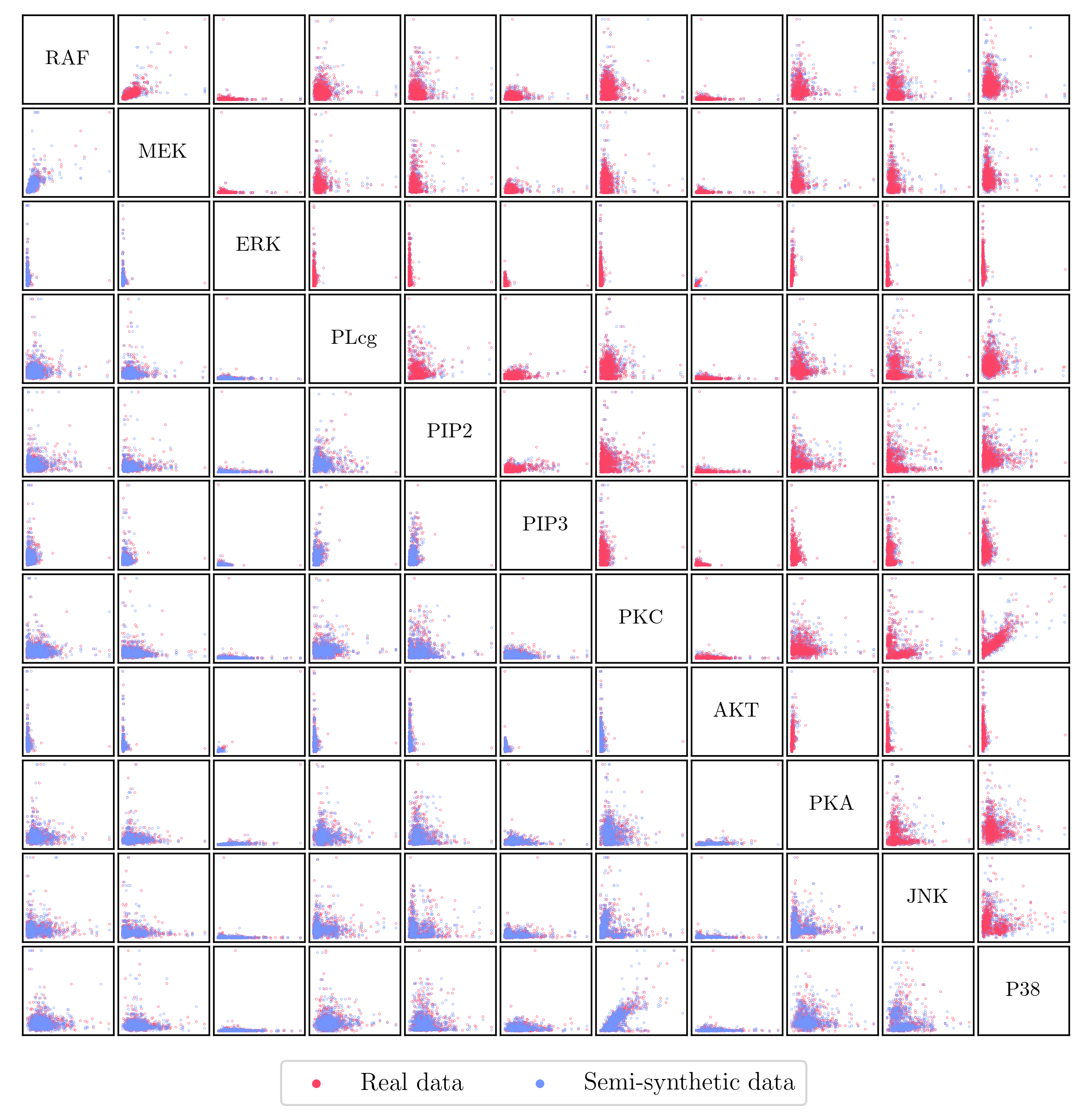
Figure 5: Pairwise observations of all variables in the Sachs data set, for the real (red) and semi-synthetic (blue) data. The conditional distributions of the semi-synthetic data set closely follow those of the real data set, and both exhibit a high degree of non-linearity.

F Additional Figures

References

- Brouillard et al. (2020) Philippe Brouillard, Sébastien Lachapelle, Alexandre Lacoste, Simon Lacoste-Julien, and Alexandre Drouin. Differentiable causal discovery from interventional data. Advances in Neural Information Processing Systems, 33:21865–21877, 2020.
- Bühlmann (2020) Peter Bühlmann. Invariance, causality and robustness. Statistical Science, 35(3):404–426, 2020.
- Bühlmann et al. (2014) Peter Bühlmann, Jonas Peters, and Jan Ernest. CAM: Causal additive models, high-dimensional order search and penalized regression. The Annals of Statistics, 42(6):2526 – 2556, 2014.
- Ćevid et al. (2020) Domagoj Ćevid, Loris Michel, Jeffrey Näf, Nicolai Meinshausen, and Peter Bühlmann. Distributional random forests: Heterogeneity adjustment and multivariate distributional regression. arXiv preprint arXiv:2005.14458, 2020.
- Chickering (1995) David Maxwell Chickering. A transformational characterization of equivalent Bayesian network structures. In Proceedings of the Eleventh Conference on Uncertainty in Artificial Intelligence, pages 87–98, 1995.
- Chickering (2002) David Maxwell Chickering. Optimal structure identification with greedy search. Journal of Machine Learning Research, 3(Nov):507–554, 2002.
- Chickering (2020) David Maxwell Chickering. Statistically efficient greedy equivalence search. In Proceedings of the Thirty-Sixth Conference on Uncertainty in Artificial Intelligence, pages 241–249, 2020.
- Chickering and Meek (2015) David Maxwell Chickering and Christopher Meek. Selective greedy equivalence search: finding optimal Bayesian networks using a polynomial number of score evaluations. In Proceedings of the Thirty-First Conference on Uncertainty in Artificial Intelligence, pages 211–219, 2015.
- Didelez (2005) Vanessa Didelez. Statistical causality. Consilience Interdisplinary Communications, 2996:114–120, 2005.
- Eberhardt (2007) Frederick Eberhardt. Causation and intervention. PhD Thesis, Carnegie Mellon University, 2007.
- Eberhardt and Scheines (2007) Frederick Eberhardt and Richard Scheines. Interventions and causal inference. Philosophy of Science, 74(5):981–995, 2007.
- Faria et al. (2022) Gonçalo Rui Alves Faria, Andre Martins, and Mario A. T. Figueiredo. Differentiable causal discovery under latent interventions. In Proceedings of the First Conference on Causal Learning and Reasoning, pages 253–274, 2022.
- Gamella and Heinze-Deml (2020) Juan L. Gamella and Christina Heinze-Deml. Active invariant causal prediction: experiment selection through stability. Advances in Neural Information Processing Systems, 33:15464–15475, 2020.
- Ghassami et al. (2017) AmirEmad Ghassami, Saber Salehkaleybar, Negar Kiyavash, and Kun Zhang. Learning causal structures using regression invariance. Advances in Neural Information Processing Systems, 30:3015–3025, 2017.
- Gopnik et al. (2004) Alison Gopnik, Clark Glymour, David M. Sobel, Laura E. Schulz, Tamar Kushnir, and David Danks. A theory of causal learning in children: causal maps and Bayes nets. Psychological Review, 111(1):3, 2004.
- Hägele et al. (2022) Alexander Hägele, Jonas Rothfuss, Lars Lorch, Vignesh Ram Somnath, Bernhard Schölkopf, and Andreas Krause. Bacadi: Bayesian causal discovery with unknown interventions. arXiv preprint arXiv:2206.01665, 2022.
- Hauser and Bühlmann (2012) Alain Hauser and Peter Bühlmann. Characterization and greedy learning of interventional Markov equivalence classes of directed acyclic graphs. Journal of Machine Learning Research, 13(Aug):2409–2464, 2012.
- Hauser and Bühlmann (2014) Alain Hauser and Peter Bühlmann. Two optimal strategies for active learning of causal models from interventional data. International Journal of Approximate Reasoning, 55(4):926–939, 2014.
- Hauser and Bühlmann (2015) Alain Hauser and Peter Bühlmann. Jointly interventional and observational data: estimation of interventional Markov equivalence classes of directed acyclic graphs. Journal of the Royal Statistical Society: Series B (Statistical Methodology), 77(1):291–318, 2015.
- Heinze-Deml and Meinshausen (2021) Christina Heinze-Deml and Nicolai Meinshausen. Conditional variance penalties and domain shift robustness. Machine Learning, 110(2):303–348, 2021.
- Heinze-Deml et al. (2018) Christina Heinze-Deml, Jonas Peters, and Nicolai Meinshausen. Invariant causal prediction for nonlinear models. Journal of Causal Inference, 6(2), 2018.
- Hoyer et al. (2009) Patrik O. Hoyer, Dominik Janzing, Joris M. Mooij, Jonas Peters, and Bernhard Schölkopf. Nonlinear causal discovery with additive noise models. Advances in Neural Information Processing Systems, 22:689–696, 2009.
- Jaber et al. (2020) Amin Jaber, Murat Kocaoglu, Karthikeyan Shanmugam, and Elias Bareinboim. Causal discovery from soft interventions with unknown targets: characterization and learning. Advances in Neural Information Processing Systems, 33:9551–9561, 2020.
- Ke et al. (2019) Nan Rosemary Ke, Olexa Bilaniuk, Anirudh Goyal, Stefan Bauer, Hugo Larochelle, Bernhard Schölkopf, Michael C. Mozer, Chris Pal, and Yoshua Bengio. Learning neural causal models from unknown interventions. arXiv preprint arXiv:1910.01075, 2019.
- Lachapelle et al. (2019) Sébastien Lachapelle, Philippe Brouillard, Tristan Deleu, and Simon Lacoste-Julien. Gradient-based neural dag learning. arXiv preprint arXiv:1906.02226, 2019.
- Magliacane et al. (2016) Sara Magliacane, Tom Claassen, and Joris M. Mooij. Ancestral causal inference. Advances in Neural Information Processing Systems, 29:4473–4481, 2016.
- Meek (1995) Christopher Meek. Causal inference and causal explanation with background knowledge. In Proceedings of the Eleventh Conference on Uncertainty in Artificial Intelligence, pages 403–410, 1995.
- Meinshausen et al. (2016) Nicolai Meinshausen, Alain Hauser, Joris M. Mooij, Jonas Peters, Philip Versteeg, and Peter Bühlmann. Methods for causal inference from gene perturbation experiments and validation. Proceedings of the National Academy of Sciences, 113(27):7361–7368, 2016.
- Mooij and Heskes (2013) Joris M. Mooij and Tom Heskes. Cyclic causal discovery from continuous equilibrium data. In Proceedings of the Twenty-Ninth Conference on Uncertainty in Artificial Intelligence, pages 431–439, 2013.
- Mooij et al. (2022) Joris M. Mooij, Sara Magliacane, and Tom Claassen. Joint causal inference from multiple contexts. Journal of Machine Learning Research, 21(Jun):1–108, 2022.
- Muentener and Bonawitz (2017) Paul Muentener and Elizabeth Bonawitz. The development of causal reasoning. In The Oxford Handbook of Causal Reasoning. Oxford University Press, 2017.
- Nandy et al. (2018) Preetam Nandy, Alain Hauser, and Marloes Maathuis. High-dimensional consistency in score-based and hybrid structure learning. The Annals of Statistics, 46(6A):3151–3183, 2018.
- Ng et al. (2020) Ignavier Ng, AmirEmad Ghassami, and Kun Zhang. On the role of sparsity and dag constraints for learning linear dags. Advances in Neural Information Processing Systems, 33:17943–17954, 2020.
- Pearl (1988) Judea Pearl. Probabilistic Reasoning in Intelligent Systems: Networks of Plausible Inference. Morgan Kaufmann, 1988.
- Pearl (2009a) Judea Pearl. Causal inference in statistics: An overview. Statistics Surveys, 3:96–146, 2009a.
- Pearl (2009b) Judea Pearl. Causality. Cambridge university press, 2009b.
- Peters and Bühlmann (2013) Jonas Peters and Peter Bühlmann. Identifiability of Gaussian structural equation models with equal error variances. Biometrika, 101(1):219–228, 2013.
- Peters et al. (2011) Jonas Peters, Joris M. Mooij, Dominik Janzing, and Bernhard Schölkopf. Identifiability of causal graphs using functional models. In Proceedings of the Twenty-Seventh Conference on Uncertainty in Artificial Intelligence, pages 589–598, 2011.
- Peters et al. (2016) Jonas Peters, Peter Bühlmann, and Nicolai Meinshausen. Causal inference by using invariant prediction: identification and confidence intervals. Journal of the Royal Statistical Society: Series B (Statistical Methodology), 78(5):947–1012, 2016.
- Peters et al. (2017) Jonas Peters, Dominik Janzing, and Bernhard Schölkopf. Elements of Causal Inference: Foundations and Learning Algorithms. MIT press, 2017.
- Pfister et al. (2019) Niklas Pfister, Peter Bühlmann, and Jonas Peters. Invariant causal prediction for sequential data. Journal of the American Statistical Association, 114(527):1264–1276, 2019.
- Pfister et al. (2021) Niklas Pfister, Evan G. Williams, Jonas Peters, Ruedi Aebersold, and Peter Bühlmann. Stabilizing variable selection and regression. The Annals of Applied Statistics, 15(3):1220–1246, 2021.
- Reisach et al. (2021) Alexander Reisach, Christof Seiler, and Sebastian Weichwald. Beware of the simulated dag! causal discovery benchmarks may be easy to game. Advances in Neural Information Processing Systems, 34:27772–27784, 2021.
- Rothenhäusler et al. (2021) Dominik Rothenhäusler, Nicolai Meinshausen, Peter Bühlmann, and Jonas Peters. Anchor regression: Heterogeneous data meet causality. Journal of the Royal Statistical Society Series B (Statistical Methodology), 83(2):215–246, 2021.
- Sachs et al. (2005) Karen Sachs, Omar Perez, Dana Pe’er, Douglas A. Lauffenburger, and Garry P. Nolan. Causal protein-signaling networks derived from multiparameter single-cell data. Science, 308(5721):523–529, 2005.
- Seng et al. (2022) Jonas Seng, Matej Zečević, Devendra Singh Dhami, and Kristian Kersting. Tearing apart notears: Controlling the graph prediction via variance manipulation. arXiv preprint arXiv:2206.07195, 2022.
- Shimizu et al. (2006) Shohei Shimizu, Patrik O. Hoyer, Aapo Hyvärinen, and Antti Kerminen. A linear non-Gaussian acyclic model for causal discovery. Journal of Machine Learning Research, 7(Oct):2003–2030, 2006.
- Solus et al. (2021) Liam Solus, Yuhao Wang, and Caroline Uhler. Consistency guarantees for greedy permutation-based causal inference algorithms. Biometrika, 108(4):795–814, 2021.
- Spirtes et al. (1999) Peter Spirtes, Christopher Meek, and Thomas Richardson. An algorithm for causal inference in the presence of latent variables and selection bias. Computation, Causation, and Discovery, 21:211–252, 1999.
- Spirtes et al. (2000) Peter Spirtes, Clark N. Glymour, Richard Scheines, and David Heckerman. Causation, Prediction, and Search. MIT press, 2000.
- Squires et al. (2020) Chandler Squires, Yuhao Wang, and Caroline Uhler. Permutation-based causal structure learning with unknown intervention targets. In Proceedings of the Thirty-Sixth Conference on Uncertainty in Artificial Intelligence, pages 1039–1048, 2020.
- Subbaswamy et al. (2019) Adarsh Subbaswamy, Peter Schulam, and Suchi Saria. Preventing failures due to dataset shift: Learning predictive models that transport. In Proceedings of the Twenty-Second International Conference on Artificial Intelligence and Statistics, pages 3118–3127, 2019.
- Taeb et al. (2021) Armeen Taeb, Juan L. Gamella, Christina Heinze-Deml, and Peter Bühlmann. Perturbations and causality in Gaussian latent variable models. arXiv preprint arXiv:2101.06950, 2021.
- Tian and Pearl (2001) Jin Tian and Judea Pearl. Causal discovery from changes. In Proceedings of the Seventeenth Conference on Uncertainty in Artificial Intelligence, pages 512–521, 2001.
- van de Geer (2000) Sara van de Geer. Empirical Processes in M-estimation. Cambridge university press, 2000.
- van de Geer and Bühlmann (2013) Sara van de Geer and Peter Bühlmann. -penalized maximum likelihood for sparse directed acyclic graphs. The Annals of Statistics, 41(2):536–567, 2013.
- Verma and Pearl (1990) Thomas Verma and Judea Pearl. Equivalence and synthesis of causal models. In Proceedings of the Sixth Conference on Uncertainty in Artificial Intelligence, pages 255–270, 1990.
- Wang et al. (2017) Yuhao Wang, Liam Solus, Karren Yang, and Caroline Uhler. Permutation-based causal inference algorithms with interventions. Advances in Neural Information Processing Systems, 31:5824–5833, 2017.
- Yang et al. (2018) Karren Yang, Abigail Katcoff, and Caroline Uhler. Characterizing and learning equivalence classes of causal dags under interventions. In Proceedings of the Thirty-Fifth International Conference on Machine Learning, pages 5541–5550, 2018.
- Yu et al. (2019) Yue Yu, Jie Chen, Tian Gao, and Mo Yu. Dag-gnn: dag structure learning with graph neural networks. In Proceedings of the Thirty-Sixth International Conference on Machine Learning, pages 7154–7163, 2019.
- Zhang (2008) Jiji Zhang. On the completeness of orientation rules for causal discovery in the presence of latent confounders and selection bias. Artificial Intelligence, 172(16-17):1873–1896, 2008.
- Zhang et al. (2011) Kun Zhang, Jonas Peters, Dominik Janzing, and Bernhard Schölkopf. Kernel-based conditional independence test and application in causal discovery. In Proceedings of the Twenty-Seventh Conference on Uncertainty in Artificial Intelligence, pages 804–813, 2011.
- Zhang et al. (2017) Kun Zhang, Biwei Huang, Jiji Zhang, Clark Glymour, and Bernhard Schölkopf. Causal discovery from nonstationary/heterogeneous data: Skeleton estimation and orientation determination. In Proceedings of the Twenty-Sixth International Joint Conference on Artificial Intelligence, volume 2017, pages 1347–1353, 2017.
- Zheng et al. (2018) Xun Zheng, Bryon Aragam, Pradeep K. Ravikumar, and Eric P Xing. Dags with no tears: continuous optimization for structure learning. Advances in Neural Information Processing Systems, 31:9492–9503, 2018.
- Zheng et al. (2020) Xun Zheng, Chen Dan, Bryon Aragam, Pradeep Ravikumar, and Eric Xing. Learning sparse nonparametric dags. In Proceedings of the Twenty-Third International Conference on Artificial Intelligence and Statistics, pages 3414–3425, 2020.