Chandrasekhar Mass Limit of White Dwarfs in Modified Gravity

Abstract

We investigate the Chandrasekhar mass limit for white dwarfs in various models of $f(R)$ gravity. Two equations of state for stellar matter are used: simple relativistic polytropic equation with polytropic index $n=3$ and the realistic Chandrasekhar equation of state. For calculations it is convenient to use the equivalent scalar-tensor theory in the Einstein frame and then to return in the Jordan frame picture. For white dwarfs we can neglect terms containing relativistic effects from General Relativity and we consider the reduced system of equations. Its solution for any model of $f(R)=R+\beta R^{m}$ ($m\geq 2$, $\beta>0$) gravity leads to the conclusion that the stellar mass decreases in comparison with standard General Relativity. For realistic equations of state we find that there is a value of the central density for which the mass of white dwarf peaks. Therefore, in frames of modified gravity there is lower limit on the radius of stable white dwarfs and this minimal radius is greater than in General Relativity.

1 Introduction

Modified gravity in its various forms (Capozziello & Laurentis, 2011; Capozziello & Faraoni, 2011; Nojiri, Odintsov & Oikonomou, 2017; Nojiri & Odintsov, 2011; Cruz-Dombriz & Saez-Gomez, 2012; Olmo, 2011; Dimopoulos, 2021) describes successfully and in a minimal way the late-time acceleration of the universe (Perlmutter et al., 1999; Riess et al., 1998, 2004) and in many cases, the unification of the inflationary era with the early-time acceleration is possible (Nojiri & Odintsov, 2003). Although the most successful model for the cosmological acceleration is the $\Lambda$-Cold-Dark-Matter ($\Lambda$CDM) model, but it has several shortcomings from the theoretical physics viewpoint. Primarily one needs to explain the so called cosmological constant problem i.e. the very large discrepancy between observed value of $\Lambda$ term and its value predicted by any quantum field theories (Weinberg, 1989). Another way to describe cosmological acceleration in frames of General Relativity (GR) is the introduction of a scalar field. Analysis of the Planck observational data leads to conclusion that such field may be phantom field with negative kinetic terms, since the dark energy equation of state (EoS) parameter is allowed to have values marginally smaller than $-1$. Phantom fields are very problematic from a quantum field theory perspective.

In modified gravity we can explain not only data based on standard candles, but also microwave background anisotropy (Spergel et al., 2003), shear due to the gravitational weak lensing (Schimdt, et al., 2007), data about absorption lines in Lyman-a-forest (McDonald, et al., 2006) and other without cosmological constant or phantom scalars.

However, when considering modifications of GR, a holistic approach compels to consider not only possible manifestations of such theories at a cosmological level, but also at an relativistic astrophysical level, also because strong gravitational regimes could be considered if GR is the weak field limit of some more complicated effective gravitational theory.

In this paper we consider possible manifestations of $f(R)$ gravity in white dwarfs. Models of white dwarfs with polytropic EoS in Palatini $f(R)$ gravity (without no extra degree of freedom for the gravitational sector) are considered in Sarmah, Kalita & Wojnar, 2022; Wojnar, 2021. Early in many papers another class of compact objects, neutron stars (NS) have been considered in connection with modified gravity (see for example, Astashenok et al., 2020, 2021; Capozziello et al., 2016; Astashenok, Capozziello & Odintsov, 2015; Astashenok & Odintsov, 2020; Arapoglu, Deliduman & Eksi, 2011; Panotopoulos, et al., 2021; Lobato et al., 2020; Oikonomou, 2021; Odintsov & Oikonomou, 2021; Katsuragawa et al., 2022, and for a recent review see Olmo, Rubiera-Garcia & Wojnar, 2020). The general feature of the solution of the modified Tolman-Oppenheimer-Volkoff equations is that scalar curvature $R$ outside the NS doesn’t drop to zero as for for GR, but asymptotically approaches zero at the spatial infinity (and from a calculational point of view at the numerical infinity). The gravitational mass inside the star’s surface, decreases in comparison with GR for same density of nuclear matter at the center of star, but contributions to the gravitational mass are obtained from regions beyond the surface of the star. For a simple $R^{2}$ gravity effective gravitational mass of NSs increases. This result can help to explain NS with large mass (Pani & Berti, 2014; Doneva et al., 2013; Horbatsch et al., 2015; Silva et al., 2015; Chew et al., 2019; Blázquez-Salcedo, Scen Khoo & Kunz, 2020; Motahar et al., 2017; Oikonomou, 2021; Odintsov & Oikonomou, 2021). In light of the relatively recent GW190814 event, modified gravity serves as a cutting edge probable description of nature in limits where GR needs to be supplemented by a Occam’s razor compatible theory.

The density and the scalar curvature in central areas of white dwarfs of course are not so large as inside NSs. But radii of white dwarfs are two or three orders of magnitude larger and therefore some measurable effect may appear. In Newtonian gravity and for polytropic equation of state equations describing stars equilibrium, give well-known Lane-Emden equation. From calculations it follows that we can neglect relativistic effects on Newtonian background, but is this true for possible influence of modified gravity? The second important question is existence of stable stars in modified gravity for realistic EoSs, for the branch of stable stellar configurations $dM/d\rho_{c}>0$ where $\rho_{c}$ is central density. In the case of Chandrasekhar EoS mass increases with central density. Although for very large density ($\rho_{c}\sim 10^{10}$ g/cm³) this EoS is not applicable it is interesting to investigate the question about stability in modified gravity. Since the scalar curvature is relatively small one can expect that the function $f(R)$ can be represented as a power series in $R$. Therefore, in first turn we should consider a simple model of power-law gravity with an additional term $\sim R^{l}$ to scalar curvature.

The structure of this paper is as follows: In sections II and III we briefly consider Tolman-Oppenheimer-Volkoff equations in GR and $f(R)$ gravity. We can neglect relativistic terms for white dwarfs in the first case and obtain well-known Lane-Emden equation for polytropic EoSs. For $f(R)$ gravity it is convenient to use Einstein frame and the corresponding scalar-tensor theory. Neglecting same relativistic terms we obtain a reduced system of equations which is easier to numerical analysis. Then we compare the two approaches to solve this system for a simple $R^{2}$ gravity using relativistic polytropic EoS with polytropic index $n=3$. Firstly, we can use an approximation for the scalar field. In this case, the scalar field decreases as the density of the star decreases and drops to zero on star surface. Stellar mass decreases in comparison with GR. These results do not change qualitatively if we solve the reduced system without any approximation. Realistic Chandrasekhar EoS is considered in Section V for $R^{2}$ gravity. Finally, we investigate the mass limit for white dwarfs in another model of $f(R)$ gravity for a polytropic EoS. Assuming a perturbative solution for the scalar field, one can obtain the analog of Lane-Emden equation and formulate requirements to gravity model at which the Chandrasekhar mass limit increases or decreases.

2 Tolman-Oppenheimer-Volkoff Equations in GR

For relativistic non-rotating stars in equilibrium the following equations should be satisfied:

$$\frac{dm}{dr}=4\pi\rho r^{2},$$ (1)

$$\frac{dp}{dr}=-(\rho+p)\frac{m+4\pi pr^{3}}{r^{2}\left(1-\frac{2m}{r}\right)}.$$ (2)

where $\rho$ and $p$ are the density and the pressure of stellar matter respectively. Function $m$ is the gravitational mass enclosed in a sphere with radius $r$. Here we use natural system of units in which velocity of light and gravitational constant are $c=G=1$.

Dense matter in white dwarfs can be described by simple polytropic equation of state namely,

$$p=K\rho^{1+1/n}\,,$$ (3)

where $K$, $n$ are constants. One should note that the pressure and the density have the same dimensions in natural system of units. For polytropic EoSs one can obtain simple equations for dimensionless quantities and investigate the properties of the solutions of the TOV equations.

Let’s define the following dimensionless functions $\theta$ and $\mu$ and the coordinate variable $x$:

$$\rho=\rho_{c}\theta^{n},\quad m=\mu\rho_{c}a^{3},\quad r=ax,$$

where the length parameter $a$ is,

$$a=\left(\frac{(n+1)K\rho_{c}^{1/n-1}}{4\pi}\right)^{1/2}.$$

In terms of the dimensionless variables, the first equation is equivalent to,

$$\frac{d\mu}{dx}=4\pi x^{2}\theta^{n},$$ (4)

and the second equation can be reduced to,

$$\frac{1}{1+4\pi\beta\theta/(n+1)}\frac{d\theta}{dx}=-\frac{1}{4\pi}\frac{\mu+16\pi^{2}(n+1)^{-1}x^{3}\beta\theta^{n+1}}{x(x-2\beta\mu)}.$$ (5)

The dimensionless parameter $\beta$ is,

$$\beta=\rho_{c}a^{2}=\frac{n+1}{4\pi}K\rho_{c}^{1/n}<<1\,,$$

and is very small for the corresponding densities in white dwarfs. If we consider relativistic electrons ($\rho_{c}>>10^{6}$ g/cm³) then $n=3$ and

$$K=1.2435\times 10^{15}/\mu_{e}^{4/3}$$

in CGS-system. Here $\mu_{e}$ is average molecular weight per one electron. For $\mu_{e}=2$ we have that,

$$\beta=3.76\times 10^{-5}\left(\frac{\rho_{c}[\mbox{g/cm}^{3}]}{10^{7}}\right)^{1/3}$$

If we neglect terms containing $\beta$ in Eqs. (4), (5) we obtain well-known Lane-Emden equation:

$$\frac{d}{dx}\left(x^{2}\frac{d\theta}{dx}\right)=-x^{2}\theta^{n}.$$ (6)

For the case $n=3$, the mass of the star does not depend on the central density and $\mu(x_{f})=25.362$ for $x_{f}=6.896$. This corresponds to the Chandrasekhar limit of white dwarf mass $M=1.456M_{\odot}$. By taking into account relativistic terms, the results changes negligibly.

3 Spherically symmetric stellar configurations in f(R)-gravity

If we consider $f(R)$ gravity, one needs to replace the standard Einstein-Hilbert action which contains the scalar curvature $R$ by the some function of curvature $f(R)$:

$$S=\frac{1}{16\pi}\int d^{4}x\sqrt{-g}f(R)+S_{{\rm matter}}.$$ (7)

Here $g$ is determinant of the metric $g_{\mu\nu}$ and $S_{\rm matter}$ is the action of the standard perfect fluid matter.

The spherically symmetric metric for static star is

$$ds^{2}=-e^{2\psi}dt^{2}+e^{2\lambda}dr^{2}+r^{2}d\Omega^{2},$$ (8)

where $\psi$ and $\lambda$ are two independent functions of the radial coordinate $r$.

For our purposes it is useful to consider scalar-tensor theory of gravity which is equivalent to $f(R)$ gravity. The equivalent action for gravitational field in the Einstein frame is

$$S_{g}=\frac{1}{16\pi}\int d^{4}x\sqrt{-g}\left(\Phi R-U(\Phi)\right).$$ (9)

where the scalar field is $\Phi=f^{\prime}(R)$ and the potential is $U(\Phi)=Rf^{\prime}(R)-f(R)$. Making transformation of metric $\tilde{g}_{\mu\nu}=\Phi g_{\mu\nu}$ one write the action in the Einstein frame,

$$S_{g}=\frac{1}{16\pi}\int d^{4}x\sqrt{-\tilde{g}}\left(\tilde{R}-2\tilde{g}^{\mu\nu}\partial_{\mu}\phi\partial_{\nu}\phi-4V(\phi)\right),$$ (10)

where $\phi=\sqrt{3}\ln\Phi/2$ and the redefined potential in the Einstein frame is $V(\phi)=\Phi^{-2}(\phi)U(\Phi(\phi))/4$.

Intervals in Einstein and Jordan frames are linked by the relation

$$d\tilde{s}^{2}=\Phi ds^{2}=-e^{2\tilde{\psi}}d{t}^{2}+e^{2\tilde{\phi}}{\tilde{dr}}^{2}+\tilde{r}^{2}d\Omega^{2}.$$ (11)

Here we write $d\tilde{s}^{2}$ in form equivalent to (8) but with different functions $\tilde{\psi}$ and $\tilde{\lambda}$.

From Eq. (11) we have that $\tilde{r}^{2}=\Phi r^{2}$ and $e^{2\tilde{\psi}}=\Phi e^{2\psi}$. Combining it with equality,

$$\Phi e^{2\lambda}dr^{2}=e^{2\tilde{\lambda}}d\tilde{r}^{2}$$

we obtain that,

$$e^{-2\lambda}=e^{-2\tilde{\lambda}}\left(1-\tilde{r}\phi^{\prime}(\tilde{r})/\sqrt{3}\right)^{2}.$$

Gravitational mass $m(r)$ is defined in Jordan frame as,

$$m(r)=\frac{r}{2}\left(1-e^{-2\lambda}\right).$$ (12)

We can define function $\tilde{m}(\tilde{r})$ by the same relation,

$$\tilde{m}(\tilde{r})=\frac{\tilde{r}}{2}\left(1-e^{-2\tilde{\lambda}}\right).$$

Note that $\tilde{m}(\tilde{r})$ is not the gravitational mass measured by an observer. But the measured gravitational mass $m(r)$ can be obtained from a simple relation $\tilde{m}(\tilde{r})$ as

$$m(\tilde{r})=\frac{\tilde{r}}{2}\left(1-\left(1-\frac{2\tilde{m}}{\tilde{r}}\right)\left(1-\tilde{r}\phi^{\prime}(\tilde{r})/\sqrt{3}\right)^{2}\right)e^{-\phi/\sqrt{3}}$$ (13)

The resulting equations for the metric functions $\tilde{\lambda}$ and $\tilde{\psi}$ are very similar to the TOV equations with redefined energy and pressure, and with additional terms with the energy density and pressure of the scalar field $\phi$ being:

$$\frac{1}{\tilde{r}^{2}}\frac{d\tilde{m}}{d\tilde{r}}=4\pi e^{-4\phi/\sqrt{3}}\rho+\frac{1}{2}\left(1-\frac{2\tilde{m}}{\tilde{r}}\right)\left(\frac{d\phi}{d\tilde{r}}\right)^{2}+V(\phi),$$ (14)

$$\frac{1}{p+\rho}\frac{dp}{d\tilde{r}}=-\frac{\tilde{m}+4\pi e^{-4\phi/\sqrt{3}}p\tilde{r}^{3}}{\tilde{r}(\tilde{r}-2\tilde{m})}-\frac{\tilde{r}}{2}\left(\frac{d\phi}{d\tilde{r}}\right)^{2}+$$ (15)

$$+\frac{\tilde{r}^{2}V(\phi)}{\tilde{r}-2\tilde{m}}+\frac{1}{\sqrt{3}}\frac{d\phi}{d\tilde{r}},$$

The second equation is obtained with using condition of hydrostatic equilibrium,

$$\frac{dp}{d\tilde{r}}=-(\rho+p)\left(\frac{d\psi}{d\tilde{r}}-\frac{1}{\sqrt{3}}\frac{d\phi}{d\tilde{r}}\right).$$ (16)

Finally, one needs to add the equation of the scalar field obtained by taking the trace of Einstein equations:

$$\triangle_{\tilde{r}}\phi-\frac{dV(\phi)}{d\phi}=-\frac{4\pi}{\sqrt{3}}e^{-4\phi/\sqrt{3}}(\rho-3p).$$ (17)

Here $\triangle_{\tilde{r}}$ is radial part of Laplace-Beltrami operator for the metric (11):

$$\triangle_{\tilde{r}}=e^{-2\tilde{\lambda}}\left(\frac{2}{r}+\frac{d\psi}{dr}-\frac{d\lambda}{dr}\right)\frac{d}{dr}+e^{-2\tilde{\lambda}}\frac{d^{2}}{dr^{2}}.$$

We rewrite equations (14), (15), (17) in terms of dimensionless variables introduced earlier:

$$\frac{d\tilde{\mu}}{dx}=4\pi\tilde{x}^{2}\theta^{n}\mathrm{e}^{-4\phi/\sqrt{3}}+\frac{\tilde{x}^{2}}{\beta}\left(\frac{1}{2}\left(1-\frac{2\beta\tilde{\mu}}{\tilde{x}}\right)\left(\frac{d\phi}{d\tilde{x}}\right)^{2}+v(\phi)\right),$$ (18)

$$\frac{1}{1+4\pi\beta\theta/(n+1)}\frac{d\theta}{d\tilde{x}}=-\frac{1}{4\pi}\frac{\tilde{\mu}+16\pi^{2}\beta\theta^{n+1}\tilde{x}^{3}e^{-4\phi/\sqrt{3}}}{\tilde{x}(\tilde{x}-2{\beta}\tilde{\mu})}-$$ (19)

$$-\frac{\tilde{x}^{2}}{4\pi\beta(\tilde{x}-2\beta\tilde{\mu})}\left(\frac{1}{2}\left(1-\frac{2\beta\tilde{\mu}}{\tilde{x}}\right)\left(\frac{d\phi}{d\tilde{x}}\right)^{2}-v(\phi)\right)+\frac{1}{4\sqrt{3}\pi\beta}\frac{d\phi}{d\tilde{x}}$$

Here we introduced the dimensionless potential of scalar field $v(\phi)$,

$$v(\phi)=a^{2}V(\phi).$$

The equation for the scalar field $\phi$ after some calculations can be written in the following form,

$$\left(1-\frac{2\beta\tilde{\mu}}{\tilde{x}}\right)\left(\frac{d^{2}\phi}{d\tilde{x}^{2}}+\left(\frac{2}{\tilde{x}}-\frac{4\pi\beta}{1+4\pi\beta/(n+1)}\frac{d\theta}{d\tilde{x}}+\frac{1}{\sqrt{3}}\frac{d\phi}{d\tilde{x}}\right)\frac{d\phi}{d\tilde{x}}\right)+$$ (20)

$$+\left(\frac{\beta\tilde{\mu}}{\tilde{x}^{2}}-\frac{\beta}{\tilde{x}}\frac{d\tilde{\mu}}{d\tilde{x}}\right)\frac{d\phi}{d\tilde{x}}-\frac{dv}{d\phi}=$$

$$=-\frac{4\pi\beta}{\sqrt{3}}e^{-4\phi/\sqrt{3}}\theta^{n}\left(1-12\pi\beta\theta/(n+1)\right).$$

Equations (18), (19) with (20) can be integrated numerically for various values of the parameter $n$. From previous analysis of TOV equations in a case of white dwarfs we know that terms proportional to small parameter $\beta$ do not affect considerably the solution. Assuming the same in a case of modified gravity we can study the“reduced” system of equations, leaving only terms with scalar field in which parameter $\beta$ in denominator:

$$\frac{d\tilde{\mu}}{dx}=4\pi\tilde{x}^{2}\theta^{n}\mathrm{e}^{-4\phi/\sqrt{3}}+\frac{\tilde{x}^{2}}{\beta}\left(\frac{1}{2}\left(\frac{d\phi}{d\tilde{x}}\right)^{2}+v(\phi)\right),$$ (21)

$$\frac{d\theta}{d\tilde{x}}=-\frac{\tilde{\mu}}{4\pi\tilde{x}^{2}}-\frac{\tilde{x}}{4\pi\beta}\left(\frac{1}{2}\left(\frac{d\phi}{d\tilde{x}}\right)^{2}-v(\phi)\right)+\frac{1}{4\sqrt{3}\pi\beta}\frac{d\phi}{d\tilde{x}}.$$ (22)

In the left hand side of Eq. (20) we also drop terms containing parameter $\beta$ and terms with square of first derivative of scalar field. In the right hand side of this equation we leave only terms with first power of $\beta$:

$$\frac{d^{2}\phi}{d\tilde{x}^{2}}+\frac{2}{\tilde{x}}\frac{d\phi}{d\tilde{x}}-\frac{dv}{d\phi}=-\frac{4\pi\beta}{\sqrt{3}}e^{-4\phi/\sqrt{3}}\theta^{n}.$$ (23)

The system of equations should be complemented by initial conditions at the center of star:

$$\theta(0)=1,\quad\tilde{\mu}(0)=0,\quad\phi(0)=\phi_{0},\quad\frac{d\phi(0)}{d\tilde{x}}=0.$$

The condition of asymptotic flatness requires that

$$\phi\rightarrow 0\quad\mbox{at}\quad x\rightarrow\infty.$$

It is convenient to analyse system of equations in the Einstein frame and then after calculations go back to the Jordan frame. We are interested mainly in effects of modified gravity and therefore we consider reduced system of equations (21), (22), (23).

4 Simple model of R2 gravity: perturbative approach and numerical integration of reduced system

Considering a simple $R^{2}$ gravity with $f(R)=R+\alpha R^{2}$ gravity we have that,

$$v(\phi)=\frac{1}{16\tilde{\alpha}}\left(1-e^{-2\phi/\sqrt{3}}\right)^{2},\quad\tilde{\alpha}=\alpha/a^{2}.$$ (24)

Usually one assumes that $\alpha>0$, otherwise model of $R^{2}$ gravity leads to instabilities. Because scalar field is very small we can expand potential $v(\phi)$ leaving only first non-zero term:

$$v(\phi)=\frac{1}{12\tilde{\alpha}}\phi^{2}.$$

Assuming that the scalar potential term is dominant and scalar field is very small we can reduce equation (23) to relation between the density and the scalar field:

$$\frac{\phi}{6\tilde{\alpha}}=\frac{4\pi\beta}{\sqrt{3}}\theta^{n}.$$ (25)

From this approximation follows that outside the star $\phi=0$ and $\frac{d\phi}{dx}=0$. Therefore, $\tilde{x}_{f}=x_{f}$ and $\tilde{\mu}(\tilde{x}_{f})={\mu}(x_{f})$.

From observations it follows that the upper limit on parameter $\alpha$ is $\sim 10^{15}$ cm². For $\alpha=10^{14}$ cm² the results of the calculations are given in Table I.

The analysis shows that the contribution of the scalar field on the pressure and the density is very negligible. Only the last term in (22) gives a considerable effect on the solution of the equations. It is very easy to understand why this happens. From the approximation (25), it follows that $d\phi/dx\sim\alpha\mathcal{O}(\beta)$ and therefore

$$\frac{1}{2}\left(\frac{d\phi}{dx}\right)^{2}\sim 10^{2}\tilde{\alpha}^{2}\mathcal{O}(\beta^{2}),\quad v(\phi)\sim 10\tilde{\alpha}\mathcal{O}(\beta^{2}).$$

The length parameter $a$ varies from $2.25\times 10^{8}$ cm for $\rho_{c}=10^{7}$ g/cm³ to $4.85\times 10^{7}$ cm for $\rho_{c}=10^{9}$ g/cm³. Therefore, even for the upper limit of the parameter $\alpha$, the dimensionless parameter $\tilde{\alpha}<1$ and the contribution of the terms in brackets in (21), (22) is $\mathcal{O}(\beta)$ i.e. it is comparable with relativistic effects from General Relativity in comparison with Newtonian gravity.

Only for sufficiently large $\tilde{\alpha}$ one can expect that the approximation (25) does not work because the square of scalar field derivative is comparable to the value with potential term.

We investigate solutions of the reduced system of equations without approximation (25) and found that account of more exact solution for scalar field increases mass of star. For $\tilde{\alpha}<0.02$ this increase is less than $0.01M_{\odot}$ in comparison to the perturbative solution. In the case of $\alpha=10^{14}$ cm² this corresponds to central densities up to $3.2\times 10^{8}$ g/cm³. For $\alpha=10^{13}$ cm², the approximation (25) can be used for central densities $\rho_{c}<10^{10}$ g/cm³. In real white dwarfs as assumed central densities are less. For $\alpha=10^{15}$ cm² one needs to solve the exact equation for the scalar field. Of course such values of the parameter $\alpha$ represent only theoretical interest because the decrease of white dwarf mass is very large in comparison with GR which is difficult to reconcile with the available observational data.

The profile of the scalar field from solution of (23) is a function decreasing with the coordinate $x$ and follows to the density profile. For illustration we plot the solution of (23) and profile of scalar field derived from (25) for various values of $\rho_{c}$ and $\alpha=10^{14}$ cm². For large $\tilde{\alpha}$, the profile of the exact solution differs significantly from the approximation. We also see that the “tale” of the scalar field outside the surface of the star is very short and this existence does not affect the stellar mass. We point out that another situation takes place in neutron stars. Density sharply drops near the surface of NS, but the scalar field decreases more slowly and therefore in $R^{2}$ gravity around surface of neutron star, a “gravitational sphere” exists with scalar curvature $R\neq 0$ (or $\phi\neq 0$ in Einstein frame). It gives contribution to gravitational mass and for high central densities and $\alpha>0$ NS mass increases.

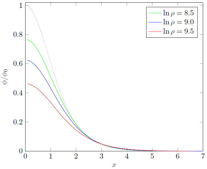
Figure 1: Profile of scalar field (solid lines) as function of dimensionless variable x in comparison with approximation (25) (black dotted line) for some central densities. Parameter $\alpha=10^{14}$ cm². $\phi_{0}$ means value of scalar field in the center of star for perturbative solution. For exact solution scalar field starts from smaller values ($\phi(0)/\phi_{0}<1$).

$\ln{\rho_{c}}$	$\tilde{\alpha},$	$\phi_{c}/\phi_{p}(0)$	$M,$	$M_{p},$
	$10^{-3}$		$M_{\odot}$	$M_{\odot}$
7	1.97	$\sim 1$	1.448	1.448
7.5	4.25	$\sim 1$	1.439	1.439
8	9.15	0.92203	1.419	1.418
8.5	19.71	0.76707	1.389	1.377
9	42.48	0.62547	1.334	1.295
9.5	91.52	0.46316	1.260	1.162

Table 1: Difference between results for stellar masses from exact solution of reduced system ($M$) and perturbative solution ($M_{p}$) for $\alpha=10^{14}$ cm². We give also corresponding values of dimensionless parameter $\tilde{\alpha}$ and the relation $\phi_{c}/\phi_{p}(0)$. Here $\phi_{c}$ is the value of scalar field in the center of star and $\phi_{p}(0)$ is the value of scalar field from perturbative approximation.

5 Realistic equation of state

The next step is to consider more realistic EoSs. We choose the Chandrasekhar EoS for stellar matter, which can be written in parametric form:

$$\rho=By^{3},$$ (26)

$$p=A\left[y(2y^{2}-3)(1+y^{2})^{1/2}+3\ln(x+(1+x^{2})^{1/2}\right],$$

$$B=9.82\times 10^{5}\mu_{e}\mbox{ g/cm}^{3},A=6.02\times 10^{22}\mbox{ dyne/cm}^{2}.$$

Again, it is useful to introduce dimensionless variables in Eqs. (14), (15). Taking into account characteristic radii and masses of white dwarfs let us define:

$$\tilde{r}=R_{e}\tilde{x},\quad\tilde{m}=M_{\odot}\tilde{\mu},$$

$$\rho=\rho_{c}\eta,\quad p=p_{c}\xi.$$

Here $R_{e}$ means radius of Earth. Restoring $G$ and $c$ in equations we obtain the following system of equations for dimensionless variables $\tilde{\mu}$, $\eta$, $\xi$ and $\phi$:

$$\frac{d\tilde{\mu}}{d\tilde{x}}=\delta 4\pi\tilde{x}^{2}e^{-4\phi/\sqrt{3}}\eta+\frac{1}{2}\frac{R_{e}}{r_{g}}\left(1-\frac{2r_{g}}{R_{e}}\frac{\tilde{\mu}}{\tilde{x}}\right)\left(\frac{d\phi}{d\tilde{x}}\right)^{2}+\frac{R_{e}}{r_{g}}v(\phi),$$ (27)

$$\frac{1}{\eta+\xi/\gamma}\frac{d\xi}{d\tilde{x}}=-\gamma\frac{r_{g}}{R_{e}}\frac{\tilde{\mu}}{\tilde{x}(\tilde{x}-2r_{g}\tilde{\mu}/R_{e})}-\delta\frac{r_{g}}{R_{e}}\frac{4\pi e^{-4\phi/\sqrt{3}}\tilde{x}^{3}\xi}{\tilde{x}(\tilde{x}-2r_{g}\tilde{\mu}/R_{e})}+$$ (28)

$$+\gamma\left(-\frac{\tilde{x}}{2}\left(\frac{d\phi}{d\tilde{x}}\right)^{2}+\frac{\tilde{x}^{2}v(\phi)}{\tilde{x}-2r_{g}\tilde{\mu}/R_{e}}+\frac{1}{\sqrt{3}}\frac{d\phi}{d\tilde{x}}\right),$$

$$\left(1-\frac{2r_{g}}{R_{e}}\frac{\tilde{\mu}}{\tilde{x}}\right)\left(\frac{d^{2}\phi}{d\tilde{x}^{2}}+\left(\frac{2}{\tilde{x}}-\frac{1}{\gamma\eta+\xi}\frac{d\xi}{dx}+\frac{1}{\sqrt{3}}\frac{d\phi}{d\tilde{x}}\right)\frac{d\phi}{d\tilde{x}}\right)+$$ (29)

$$+\frac{r_{g}}{R_{e}}\left(\frac{\tilde{\mu}}{\tilde{x}^{2}}-\frac{1}{\tilde{x}}\frac{d\tilde{\mu}}{d\tilde{x}}\right)\frac{d\phi}{d\tilde{x}}-\frac{dv}{d\phi}=-\frac{4\pi\delta}{\sqrt{3}}\frac{r_{g}}{R_{e}}e^{-4\phi/\sqrt{3}}\left(\eta-3\xi/\gamma\right),$$

where the dimensionless parameters $\delta$ and $\gamma$ are introduced:

$$\delta=\frac{\rho_{c}R_{e}^{3}}{M_{\odot}},\quad\gamma=\frac{\rho_{c}c^{2}}{p_{c}}$$

and $v(\phi)=V(\phi)R_{e}^{2}$. The parameter $r_{g}={GM_{\odot}}/{c^{2}}$ is nothing else than half of gravitational radius of Sun. Again we consider the reduced system of equations neglecting terms containing the relation $r_{g}/R_{e}<<1$ in the denominators and take into account that that the parameter $\gamma>>\delta$ for white dwarfs, and we get,

$$\frac{d\tilde{\mu}}{d\tilde{x}}=\delta 4\pi\tilde{x}^{2}e^{-4\phi/\sqrt{3}}\eta+\frac{R_{e}}{r_{g}}\left(\left(\frac{1}{2}\frac{d\phi}{d\tilde{x}}\right)^{2}+v(\phi)\right),$$ (30)

$$\frac{1}{\eta}\frac{d\xi}{d\tilde{x}}=-\gamma\frac{r_{g}}{R_{e}}\frac{\tilde{\mu}}{\tilde{x}^{2}}+\gamma\left(-\frac{\tilde{x}}{2}\left(\frac{d\phi}{d\tilde{x}}\right)^{2}+{\tilde{x}v(\phi)}+\frac{1}{\sqrt{3}}\frac{d\phi}{d\tilde{x}}\right),$$ (31)

$$\frac{d^{2}\phi}{d\tilde{x}^{2}}+\left(\frac{2}{\tilde{x}}+\frac{1}{\sqrt{3}}\frac{d\phi}{d\tilde{x}}\right)\frac{d\phi}{d\tilde{x}}-\frac{dv}{d\phi}=-\frac{4\pi\delta}{\sqrt{3}}\frac{r_{g}}{R_{e}}e^{-4\phi/\sqrt{3}}\eta.$$ (32)

As in the previous case we consider the potential for $R^{2}$ gravity and compare results from perturbative approximation for the scalar field and more exact solution of (32). The main result is the same as for relativistic polytrope: the stellar mass decreases in comparison with GR for the same central density. For large densities one needs to solve the equation for scalar field because the perturbative approximation is not valid. But it is interesting to note that in the case of $R^{2}$ gravity, the stellar mass has a maximum for some central density and then the mass decreases although in GR mass grows with density for the Chandrasekhar EoS.

In fig. 2 we depicted the mass-density relation for the interval of densities between $10^{7}$ and $10^{10}$ g/cm³ for various values of $\alpha$. These results are important for establishing the upper limit on parameter $\alpha$ in $R^{2}$ gravity. According to latest observations white dwarfs with masses $M>1.3M_{\odot}$ are very rare. Only 25 such white dwarfs are observed in vicinity of Sun System (Kilic, et al., 2021). White dwarf J1329 + 2549 is currently the most massive white dwarf known with a mass of $1.351\pm 0.006M_{\odot}$. Considering $1.35M_{\odot}$ as lower limit on maximal value for white dwarf mass and assuming that the Chandrasekhar EoS is valid, we conclude that $\alpha<10^{13}$ cm². These results lead to conclusion that GR gives satisfactory picture for white dwarfs parameters. Analyzing of white dwarfs parameters in $R^{2}$ gravity for realistic values of $\alpha$ can be performed using approximation for scalar field.

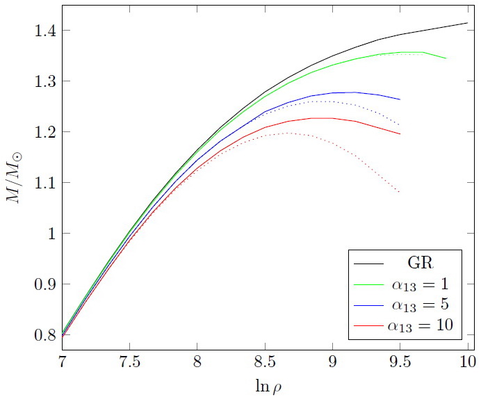
Figure 2: Mass-density relation in $R^{2}$ gravity for some $\alpha$ in comparison with GR. The dotted lines correspond to results obtained with simple approximation for scalar field. $\alpha_{13}$ means that value of $\alpha$ is given in units of $10^{13}$ cm².

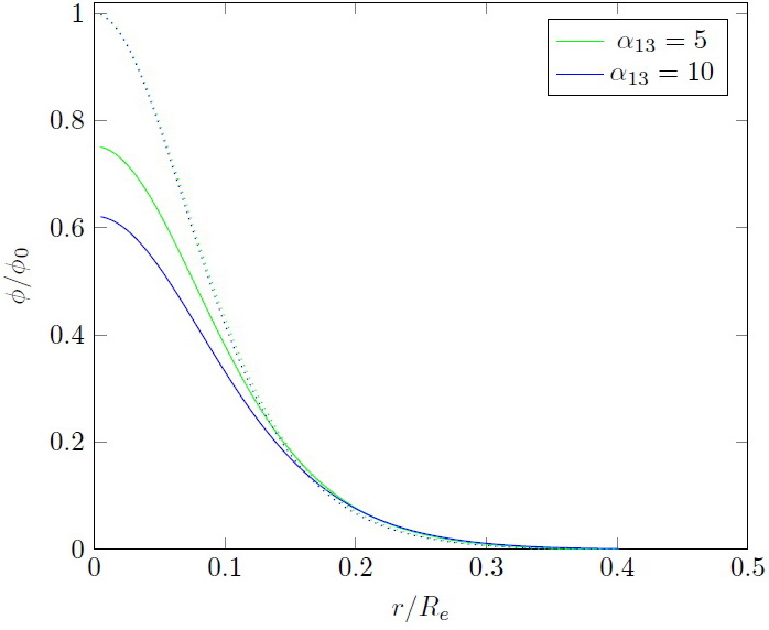
Figure 3: Profile of the scalar field (solid lines) as function of radial coordinate in comparison with approximation (25) (dotted lines) for $\rho_{c}=10^{9}$ g/cm³ and Chandrasekhar EoS.

From our results follows that for $\rho_{c}>\rho_{c}^{crit}$, white dwarfs are unstable in $R^{2}$ gravity. Critical density and minimal radius of white dwarf depends on the value of $\alpha$. In light of these results for masses and radii of white dwarfs near the Chandrasekhar limit, in principle they allow us to estimate the upper limit of $\alpha$ more precisely.

The scalar field obtained from the numerical solution of Eqs.(30), (31), (32) decreases from the center to the surface of the star in the same manner as for the case of polytropic EoS: it starts from $\phi(0)<\phi_{0}$ where $\phi_{0}$ is the central value of the perturbative solution and then follows the density profile (see Fig. 3).

6 Chandrasekhar limit of mass in another models of modified gravity

We showed that in the case of white dwarfs in $R^{2}$ gravity for realistic parameters we can neglect the derivatives of the scalar field in its field equation and use simple approximation for the scalar field. As we showed , the profile of scalar field is a monotonic function of the radial coordinate. It is interesting to investigate another model of modified gravity.

Let’s consider model with $f(R)=R+\alpha^{l-1}R^{l}$ where $l>2$. This representation is chosen so that parameter $\alpha$ has a dimension of the square of length. The potential of the scalar field theory in the corresponding equivalent scalar-tensor theory in this case is

$$V(\Phi)=D\Phi^{-2}\left(\Phi-1\right)^{\frac{l}{l-1}},\quad D=\frac{l-1}{4l^{\frac{l}{l-1}}}\alpha^{-1},\quad\Phi=e^{2\phi/\sqrt{3}}.$$ (33)

Again if the scalar field $\phi$ is very small, one can expand the expression for $V(\phi)$ and obtain,

$$V(\phi)\approx D\left(\frac{2}{\sqrt{3}}\right)^{\frac{l}{l-1}}\phi^{\frac{l}{l-1}}.$$

If the potential term dominates we can use approximation,

$$\phi\approx\frac{l(2\sqrt{3})^{l}}{4}\left(\frac{\alpha}{a^{2}}\right)^{l-1}\left(\frac{4\pi\beta}{\sqrt{3}}\right)^{l-1}\theta^{n(l-1)}.$$ (34)

The dimensionless potential and the square of the scalar field derivative in order of magnitude are,

$$v(\phi)\sim\left(\frac{\alpha}{a^{2}}\right)^{l-1}\mathcal{O}(\beta^{l}),\quad\left(\frac{d\phi}{dx}\right)^{2}\sim\left(\frac{\alpha}{a^{2}}\right)^{2(l-1)}\mathcal{O}(\beta^{2l-2})$$

One can expect that for realistic values of $\alpha/a^{2}<<1$ approximation for the scalar field is valid. And as in the case of $R^{2}$ gravity, the effects of the scalar field on the density and the pressure are negligible. Moreover, for $m\geq 3$ the effects of modified gravity will be of the next order of smallness on the parameter $\beta$ in comparison with the relativistic effects of GR on background of Newton’s gravity. The square of the scalar field derivative is an order lower in comparison with potential term for $l>2$.

Calculations for some $l>2$ show the same pattern as for $l=2$: The stellar mass decreases with increasing central density. Some results are given in Fig. 4. For $\alpha/a^{2}\sim\mathcal{O}(1)$ perturbative solution is not valid. Obviously, that for realistic Chandrasekhar EoS we obtain that stellar mass has a maximum for certain density as in the case of $R^{2}$ gravity.

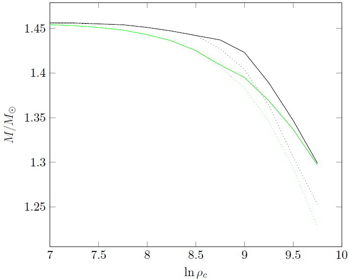
Figure 4: Mass-density relation for polytrope with $n=3$ in $R+\alpha^{l-1}R^{l}$ gravity for ($\alpha=10^{14}$ cm², $l=2.1$, green lines) and ($\alpha=5\times 10^{14}$ cm², $l=2.4$, black lines). The dotted lines correspond to results obtained with simple approximation for scalar field.

If we assume that the perturbative approximation for the scalar field is valid, then the scalar field is a monotonic function of $\phi$ because $dv/d\phi>0$ as follows from relation

$$\frac{dv}{d\phi}=\frac{4\pi\beta}{\sqrt{3}}\theta^{n}.$$ (35)

Of course $\theta$ is a monotonically decreasing function of coordinate for stable stellar configurations. Therefore, for the scalar field we can write that,

$$\phi=F(\theta)$$

where $F$ is a monotonic increasing function of its argument. The scalar field decreases with the coordinate and the potential tends to its minimum on the surface of star. The following conditions should be satisfied:

$$F(\theta)=0,\quad\frac{dF}{d\theta}=0\mbox{ for }\theta=0.$$ (36)

These conditions guarantee that scalar field and its first derivative outside of star vanish. Of course for many potentials of scalar field, the explicit relation between the scalar field and $\theta$ does not exist. The first derivative of the scalar field with respect to the coordinate $\tilde{x}$ is,

$$\frac{d\phi}{d\tilde{x}}=\frac{dF}{d\theta}\frac{d\theta}{d\tilde{x}}.$$

Equation (22) by taking into account the expression for the derivative of the scalar field and without the term $(d\phi/dx)^{2}$ can be written as,

$$\left\{1-\frac{1}{4\sqrt{3}\pi\beta}\frac{dF}{d\theta}\right\}\frac{d\theta}{dx}=-\frac{\tilde{\mu}}{4\pi\tilde{x}^{2}}+\frac{\tilde{x}}{4\pi\beta}v(\phi).$$ (37)

Then after some simple algebra, one obtains the analog of the Lane-Emden equation:

$$\frac{d}{d\tilde{x}}\left\{\tilde{x}^{2}\left\{1-\frac{1}{4\sqrt{3}\pi\beta}\frac{dF}{d\theta}\right\}\frac{d\theta}{dx}\right\}=-\tilde{x}^{2}\theta^{n}e^{-4\phi/\sqrt{3}}+$$ (38)

$$+\frac{\tilde{x}^{2}}{2\pi\beta}v(\phi)+\frac{\tilde{x}^{3}}{\sqrt{3}}\theta^{n}\frac{dF}{d\theta}\frac{d\theta}{d\tilde{x}}.$$

To obtain the scalar field potential as function of $\theta$ in frames of our approximation, one needs to take the following integral:

$$v(\theta)=\frac{4\pi\beta}{\sqrt{3}}\int_{0}^{\theta}\frac{dF}{d\theta}\theta^{n}d\theta.$$ (39)

Therefore for given $F(\theta)$ we have the potential of the scalar field in parametric form. Of course the explicit form of $v(\phi)$ can be written only for relatively simple functions $F(\theta)$. The function $\tilde{\mu}$ is defined from the following relation:

$$\tilde{\mu}(x)=-4\pi\tilde{x}^{2}\frac{d\theta(\tilde{x})}{d\tilde{x}}+\frac{\tilde{x}^{3}}{\beta}v(\theta)+\frac{\tilde{x}^{2}}{\sqrt{3}\beta}\frac{dF}{d\theta}\frac{d\theta(\tilde{x})}{d\tilde{x}}.$$ (40)

Realistic solutions of Eq.(38) for chosen $F(\theta)$ posses the same property as the solution of the Lane-Emden equation in Newtonian gravity: for some $\tilde{x}_{f}$ the function $\theta$ vanishes. This $\tilde{x}_{f}$ corresponds to surface of white dwarf. In Jordan frame $x_{f}=\tilde{x}_{f}$ because scalar field $\phi$ is zero on the star’s surface and therefore $\Phi=1$. Because the first derivative of the scalar field also vanishes on the surface, the gravitational mass of white dwarf is,

$$\mu=\tilde{\mu}(\tilde{x}_{f})$$

and therefore,

$$\mu=-4\pi\tilde{x}^{2}_{f}\frac{d\theta(\tilde{x}_{f})}{d\tilde{x}}$$

because $v(\theta)=0$ and $dF/d\theta=0$ for $\theta=0$.

Because the curvature $R$ in the case of white dwarfs is relatively small, one can propose that a realistic model of $f(R)$ gravity function $f(R)$ can be represented as series in powers of $R$:

$$f(R)=R+\alpha_{1}R^{2}+\alpha_{2}^{2}R^{3}+...$$

For $R\rightarrow 0$ and $\alpha_{1}\neq 0$, the corresponding potential of the equivalent scalar-tensor theory is,

$$v(\phi)\rightarrow\frac{\phi^{2}}{12\alpha_{1}}.$$

If $\alpha_{2}\neq 0$ and $\alpha_{1}=0$ the potential $v(\phi)\sim\phi^{3/2}$ and so on. Therefore, the first derivative of potential $dv/d\phi$ should contain terms $\sim\phi^{1/(k-1)}$, k=2,3… and monotonic function $F(\theta)$ is a sum

$$F(\theta)=s_{1}\theta^{n}+s_{2}\theta^{2n}+...$$

on interval $0\leq\theta\leq 1$. From previous results we conclude that stellar mass decreases for this function $F(\theta)$ with increasing of central density. Therefore, in frames of perturbative approach for realistic $f(R)$, one should expect that the mass of the white dwarf decreases in comparison with the GR case for the same central density.

If the function $F(\theta)$ decreases with its argument this corresponds to increasing scalar field $\phi$ from center to surface. If the scalar field is defined from (35) this leads to an increase of the potential term from the center to the surface. For $R^{2}$ gravity such situation takes place for $\alpha<0$. But this model of gravity cannot be considered as realistic because it leads to instabilities.

Therefore we conclude that in frames of perturbative approach it is impossible to construct solutions of the system (21), (22), (23) such that gravitational mass increases in comparison with GR. Increase of the value takes place only for unrealistic models of $F(R)$ gravity.

Non-monotonic function $F(\theta)$ as follows from (39) leads to that potential of scalar field should be an ambiguous function of its argument. Does a solution of (23) exists such that the derivative of the scalar field changes the sign? Let us assume that this indeed happens once. The scalar field starts from some positive value from the center of the star and reaches a minimum $\phi_{min}<0$ at some point $x_{s}$. At the vicinity of the minimum $d^{2}\phi/dx^{2}\geq 0$ and therefore $dv/d\phi>0$ the potential goes down. Then the scalar field increases and asymptotically tends to zero for large x. The asymptotical value of the scalar field outside the star should correspond to the minimum of the potential. We have therefore the situation which for example can take place for potentials of the form $u\sim\phi^{n}$ where $n=2k$, k=1,2… Scalar field reaches the minimum for some $x<x_{s}$ and develops negative values and finally approaches zero and again the minimum of the potential. But our consideration shows that for such potentials, we can construct solutions when scalar field is monotonic decreasing function from center to surface.

7 Concluding Remarks

We investigated the question about the maximal white dwarf mass limit in $f(R)$ gravity. Our analysis involved a polytropic EoS with $n=3$ and more realistic Chandrasekhar EoS. Also the equivalent scalar-tensor theory in the Einstein frame was used with the subsequent transition to the Jordan picture. For $f(R)$ gravity, one can consider the reduced system of equations, because relativistic effects of GR in the case of white dwarfs are negligible in Newtonian gravity background. In models with $f(R)=R+\alpha^{l-1}R^{l}$ for any $l\geq 2$, the mass of white dwarfs decreases in comparison with GR for $\alpha^{l-1}>0$. For realistic values of $\alpha$, the perturbative approach is valid. It is sufficient to account only potential terms in the equation for the scalar field and obtain relation for its field. For stable stars, the density should decrease from center to surface and the corresponding profile of scalar field also decreases. It is important to note that the contribution of the scalar field to energy density is around $\mathcal{O}(\beta^{l-1})$ where $\beta=\rho_{c}a^{2}G/c^{2}$ is small relativistic parameter. This contribution is comparable (for $R^{2}$ gravity) with the effect from the relativistic corrections to solutions of Lane-Emden equation or even less (for $l>2$). Applicability of the perturbative approach is defined by the relation $(\alpha/a^{2})^{l-1}$. More precise calculations show that the scalar field starts from some value $\kappa\phi_{p}(0)$ at the center of star where $0<\kappa<1$ and $\phi_{p}(0)$ is central value of the scalar field from approximation. In the case of the Chandrasekhar EoS, there exists a critical value of the central density for which the stellar mass reaches a maximum value and then decreases. Precise estimations of the maximal value of white dwarfs mass from astronomical observations has significance towards constraining the upper limit of parameter $\alpha$. If the Chandrasekhar EoS is valid, we can reconcile observational data for white dwarfs in $R^{2}$ gravity only for $\alpha<10^{13}$ cm². In comparison with NSs, it is worth to note that as believed EoS is known much more accurately. Therefore, one can hope that the possible effects of modified gravity will not disguise by uncertainty in knowledge of the equation of state. For NSs also the solution of scalar field has the following feature namely around of the star area with $\phi\neq 0$ exists. This area gives a contribution to the gravitational mass and the net effect for neutron mass with masses $M>1.5M_{\odot}$ is increasing of mass. For white dwarfs there are no significant “scalar tails” because near the surface the perturbative solution is valid with high accuracy and therefore the scalar field is defined by density mainly. In the Einstein frame it means that scalar curvature near the surface is close to its value in GR namely $R\approx 8\pi(\rho-3p)$ and drops to zero outside the star very quickly.

References

- Arapoglu, Deliduman & Eksi (2011) Arapoglu A.S., Deliduman C., Eksi K.Y., 2011, JCAP, 07, 020 [arXiv:1003.3179 [gr-qc]]
- Astashenok et al. (2020) Astashenok A.V., Capozziello S., Odintsov S.D., Oikonomou V.K., 2020, Phys. Lett. B, 811, 135910 [arXiv:2008.10884 [gr-qc]]
- Astashenok et al. (2021) Astashenok A.V., Capozziello S., Odintsov S.D., Oikonomou V.K., 2021, Phys. Lett. B, 816, 136222 [arXiv:2103.04144 [gr-qc]]
- Astashenok, Capozziello & Odintsov (2015) Astashenok A.V., Capozziello S., Odintsov S.D., 2015, JCAP, 01, 001 [arXiv:1408.3856 [gr-qc]]
- Astashenok & Odintsov (2020) Astashenok A.V., Odintsov S.D., 2020, MNRAS, 493, 78 [arXiv:2001.08504 [gr-qc]]
- Astashenok, Odintsov & Cruz-Dombriz (2017) Astashenok A.V., Odintsov S.D., de la Cruz-Dombriz A., 2017, Class. Quant. Grav., 34, 205008 [arXiv:1704.08311 [gr-qc]]
- Blázquez-Salcedo, Scen Khoo & Kunz (2020) Blázquez-Salcedo J.L., F. Scen Khoo and J. Kunz, EPL 130 (2020) no.5, 50002 [arXiv:2001.09117 [gr-qc]].
- Capozziello & Laurentis (2011) Capozziello S., De Laurentis M., 2011, Phys. Rept., 509, 167 [arXiv:1108.6266 [gr-qc]].
- Capozziello & Faraoni (2011) Capozziello S., Faraoni V. Beyond Einstein Gravity : A Survey of Gravitational Theories for Cosmology and Astrophysics, 2011, Fundam. Theor. Phys., 170, Springer, Dordrecht
- Capozziello et al. (2016) Capozziello S.,, De Laurentis M., Farinelli R., Odintsov S.D., 2016, Phys. Rev. D, 93, 023501 [arXiv:1509.04163 [gr-qc]]
- Chew et al. (2019) Chew X.Y., Kleihaus B., Kunz J., Dzhunushaliev V., Folomeev V., 2019, Phys. Rev. D, 100, 044019 [arXiv:1906.08742 [gr-qc]]
- Cruz-Dombriz & Saez-Gomez (2012) de la Cruz-Dombriz A., Saez-Gomez D., 2012, Entrp, 14, 1717 [arXiv:1207.2663 [gr-qc]].
- Dimopoulos (2021) Dimopoulos K., 2021, Introduction to Cosmic Inflation and Dark Energy, CRC Press
- Doneva et al. (2013) Doneva D.D., Yazadjiev S.S., Stergioulas N., Kokkotas K.D., 2013, Phys. Rev. D, 88, 084060 [arXiv:1309.0605 [gr-qc]]
- Horbatsch et al. (2015) Horbatsch M., Silva H.O., Gerosa D., Pani P., Berti E., Gualtieri L., Sperhake U., 2015, Class. Quant. Grav., 32, 204001 [arXiv:1505.07462 [gr-qc]]
- Katsuragawa et al. (2022) Numajiri K., Katsuragawa T., Nojiri S., 2022, PLB, 826, 136929
- Kilic, et al. (2021) Kilic M., Bergeron P., Blouin S., Bedard A., 2021, MNRAS, 503, 5397
- Lobato et al. (2020) Lobato R., Lourenço O., Moraes P.H.R.S., Lenzi C.H., de Avellar M., de Paula W., Dutra M., Malheiro M., 2020, JCAP, 12, 039 [arXiv:2009.04696 [astro-ph.HE]]
- McDonald, et al. (2006) McDonald P. et al., 2006, ApJS, 163, 80
- Motahar et al. (2017) Motahar Z., Blázquez-Salcedo J.L., Kleihaus B., Kunz J., 2017, Phys. Rev. D, 96, 064046 [arXiv:1707.05280 [gr-qc]]
- Naf & Jetzer (2010) Naf J., Jetzer P., 2010, Phys. Rev. D, 81, 104003 [arXiv:1004.2014 [gr-qc]]
- Nojiri, Odintsov & Oikonomou (2017) Nojiri S., Odintsov S.D., Oikonomou V.K., 2017, Phys. Rept., 692, 1 [arXiv:1705.11098 [gr-qc]]
- Nojiri & Odintsov (2011) Nojiri S., Odintsov S.D., 2011, Phys. Rept., 505, 59 [arXiv:1011.0544 [gr-qc]]
- Nojiri & Odintsov (2003) Nojiri S., Odintsov S.D., 2003, PhRvD, 68, 123512 [arXiv:hep-th/0307288]
- Oikonomou (2021) Oikonomou V.K., 2021, Class. Quant. Grav., 38, 175005 [arXiv:2107.12430 [gr-qc]]
- Odintsov & Oikonomou (2021) Odintsov S.D., Oikonomou V.K., 2021, Phys. Dark Univ., 32, 100805 [arXiv:2103.07725 [gr-qc]]
- Olmo (2011) Olmo G.J., 2011, IJMPD, 20, 413 [arXiv:1101.3864 [gr-qc]].
- Olmo, Rubiera-Garcia & Wojnar (2020) Olmo G.J., Rubiera-Garcia D., Wojnar A., 2020, Phys. Rept., 876, 1 [arXiv:1912.05202 [gr-qc]]
- Pani & Berti (2014) Pani P., Berti E., 2014, Phys. Rev. D, 90, 024025 [arXiv:1405.4547 [gr-qc]]
- Panotopoulos, et al. (2021) Panotopoulos G.,, Tangphati T., Banerjee A., Jasim M.K., [arXiv:2104.00590 [gr-qc]]
- Perlmutter et al. (1999) Perlmutter S. et al. [Supernova Cosmology Project Collaboration], 1999, ApJ, 517, 565 [arXiv:astro-ph/9812133]
- Riess et al. (1998) Riess A.G. et al. [Supernova Search Team Collaboration], 1998, AJ, 116, 1009 [arXiv:astro-ph/9805201]
- Riess et al. (2004) Riess A.G. et al. [Supernova Search Team Collaboration], 2004, ApJ, 607, 665 [arXiv:astro-ph/0402512]
- Sarmah, Kalita & Wojnar (2022) Sarmah L., Kalita S., Wojnar A., 2022, PhRvD, 105, 024028 [arXiv:2111.08029 [gr-qc]]
- Schimdt, et al. (2007) C. Schimdt C. et al., 2007, A&A, 463, 405
- Silva et al. (2015) Silva H.O., Macedo C.F.B., Berti E., Crispino L.C.B., 2015, Class. Quant. Grav., 32, 145008 [arXiv:1411.6286 [gr-qc]]
- Spergel et al. (2003) Spergel D.N. et al. [WMAP Collaboration], 2003, ApJS, 148, 175 [arXiv:astro-ph/0302209]
- Weinberg (1989) Weinberg S., 1989, Rev. Mod. Phys., 61, 1
- Wojnar (2021) Wojnar A., 2021, Int. J. Geom. Meth. Mod. Phys., 18, 2140006 [arXiv:2012.13927 [gr-qc]]