Soliton-mean field interaction in Korteweg-de Vries dispersive hydrodynamics

Abstract

The propagation of localized solitons in the presence of large-scale waves is a fundamental problem, both physically and mathematically, with applications in fluid dynamics, nonlinear optics and condensed matter physics. Here, the evolution of a soliton as it interacts with a rarefaction wave or a dispersive shock wave, examples of slowly varying and rapidly oscillating dispersive mean fields, for the Korteweg-de Vries equation is studied. Step boundary conditions give rise to either a rarefaction wave (step up) or a dispersive shock wave (step down). When a soliton interacts with one of these mean fields, it can either transmit through (tunnel) or become embedded (trapped) inside, depending on its initial amplitude and position. A comprehensive review of three separate analytical approaches is undertaken to describe these interactions. First, a basic soliton perturbation theory is introduced that is found to capture the solution dynamics for soliton-rarefaction wave interaction in the small dispersion limit. Next, multiphase Whitham modulation theory and its finite-gap description are used to describe soliton-rarefaction wave and soliton-dispersive shock wave interactions. Lastly, a spectral description and an exact solution of the initial value problem is obtained through the Inverse Scattering Transform. For transmitted solitons, far-field asymptotics reveal the soliton phase shift through either type of wave mentioned above. In the trapped case, there is no proper eigenvalue in the spectral description, implying that the evolution does not involve a proper soliton solution. These approaches are consistent, agree with direct numerical simulation, and accurately describe different aspects of solitary wave-mean field interaction.

1 Introduction

The interaction of small-scale dispersive waves with large-scale mean fields is a fundamental process in nonlinear wave systems with a number of applications. Traditionally, this multiscale problem involves mean fields that are either externally prescribed, such as a current, or that are induced by a finite amplitude wavetrain. A different class of nonlinear wave-mean field interactions has recently been identified in which a localized soliton or, more generally, a solitary wave, and the dynamic mean field evolve according to the same evolutionary equation [2]. A suitable equation to describe soliton-mean field interaction is the Korteweg-de Vries (KdV) equation

$$u_{t}+6uu_{x}+\varepsilon^{2}u_{xxx}=0\;,$$ (1.1)

where $t>0$ is the temporal variable, $x\in\mathbb{R}$ is the spatial variable, and $u$ is proportional to the wave amplitude. Equation (1.1) is presented in non-dimensional, scaled form with the dispersion parameter $\varepsilon>0$ measuring the relative strength of dispersion and nonlinearity. The KdV equation (1.1) admits soliton solutions whose width is proportional to $\varepsilon$.

In the small dispersion regime where $\varepsilon\ll 1$, the soliton width $\mathcal{O}(\varepsilon)$ is small relative to $\mathcal{O}(1)$ mean field spatial variation. In this context, the mean field can be slowly varying itself or can exhibit expanding, rapid, dispersive oscillations such as for a rarefaction wave (RW) or a dispersive shock wave (DSW), respectively. The term mean field applies to both the RW and DSW in the small dispersion regime because, in the RW, dispersion is negligible and the DSW is locally described by rapid oscillations with wavelength $\mathcal{O}(\varepsilon)$ whose parameters, e.g., its period-mean, change slowly, $\mathcal{O}(1)$, in comparison [3].

In [2], Whitham modulation theory [31]—an approximate method for studying modulated nonlinear wavetrains—was applied to a fluid dynamics experiment in which the free interface between an interior, buoyant, viscous fluid and an exterior, much more viscous fluid were found to exhibit solitary wave, RW, and DSW interaction dynamics [4]. In both cases of solitary wave-mean field interaction considered, two possibilities emerge. Either the solitary wave incident upon the mean field transmits or tunnels through the mean field to then propagate freely on the other side with an altered amplitude and speed. Or, the incident solitary wave remains embedded or trapped within the interior of the mean field. Sketches of these scenarios are depicted in Figure 1. Soliton transmission and trapping can also be interpreted as a form of soliton steering by the mean field.

Applications of the soliton-mean field problem range from geophysical fluid dynamics to photonic/matter waves and material science. Wherever the fundamental processes of dispersive hydrodynamics [90]—multiscale, nonlinear, dispersive waves—arise, solitons and large-scale mean fields can occur. We highlight some recent examples of environments in which solitons and DSWs have been observed and studied. If solitons and DSWs are studied separately, their interaction, and the interaction of solitons with other mean fields, are additional dynamical processes that are important to understand. In geophysical fluid dynamics, applications include gravity water waves and tsunamis [5, 6, 7, 8] as well as internal ocean waves [9, 10, 11, 12] where DSWs are also termed undular bores. There has been significant interest in the propagation of large scale mean fields in spatial and fiber nonlinear optics [13, 14, 15, 16], where fundamental DSW properties have been favorably compared with Whitham modulation theory. Superfluids are another medium in which nonlinearity due to particle interactions and dispersion resulting from quantum matter wave interference lead to solitons and DSWs [17, 18, 19, 20]. Solitons and dispersive shock waves have also been studied in stressed solids and magnetic materials [21, 22, 23].

The motivation for this review is the rapid and varied mathematical developments on this problem that have occurred within only a few years. This justifies a presentation of several mathematical approaches to the problem of soliton-mean field interaction for the KdV equation, which is arguably the simplest and most fundamental nonlinear dispersive wave model. First, we highlight the recent results obtained using Whitham modulation theory. The analysis of soliton-mean field interaction for a general class of unidirectional evolutionary equations that was initiated in [2] has since been extended to the bidirectional case for the defocusing nonlinear Schrödinger (NLS) equation [32] that includes head-on and overtaking interactions. The modified KdV equation has been used to study the interactions of new types of solitons and mean fields that come about because of nonconvex flux [37]. An extension to the two-dimensional, oblique interaction of solitons and mean fields was obtained in the context of the Kadomtsev-Petviashvili (KP) equation [24]. An analogous problem involving linear wave-mean field interaction exhibits similar behavior to soliton-mean field interaction, which was studied for the KdV equation in [35, 36]. While (m)KdV, NLS, and KP are all integrable equations, modulation theory can be applied to nonintegrable equations and has been successfully used to analyze soliton-mean field interaction in the conduit equation [2], a model of viscous core-annular fluids, and the Benjamin-Bona-Mahoney equation in [25], both nonlocal equations. The inclusion of external non-uniformities via a Hamiltonian-based modulation approach to soliton-mean field interaction for the non-integrable Gross-Pitaevskii equation was obtained in [26].

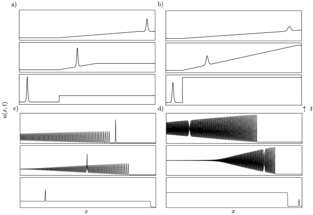
Figure 1: Soliton-mean field interaction scenarios. a) Soliton-RW tunneling. b) Soliton-RW trapping. c) Soliton-DSW tunneling. d) Soliton-DSW trapping.

While modulation theory has proven to be an effective method to analytically describe soliton-mean field interaction in a wide class of model equations, it is a formal approach in the sense that its results are not rigorously proven. A parallel set of rigorous mathematical developments for integrable equations has been achieved using the Inverse Scattering Transform (IST) [1]. The exact solutions for soliton-RW interaction in the KdV equation and soliton-DSW interaction in the focusing NLS equation were obtained in [50] and [33, 34], respectively. In these cases, small dispersion asymptotics provide strong justification for the modulation theory results. Another IST-related approach that leverages the integrability of the KdV equation is the Darboux transformation, which was used in [27] to obtain a nonlinear superposition of a soliton and rarefaction wave at $t=0$ for the transmission case.

The problem of a soliton interacting with a nonlinear wavetrain that asymptotes to a cnoidal wave in the mKdV equation was studied in [28]. This soliton-mean field problem is equivalent to a test soliton propagating through a soliton condensate, a special kind of soliton gas [29], linking soliton-mean interaction to another rapidly growing field of nonlinear wave research. In fact, soliton-cnoidal wave interaction in the KdV equation was studied some time ago [30] in which exact solutions corresponding to $N$ soliton “dislocations” to a cnoidal wave were obtained. For the $N=1$ case, we recognize these solutions as breathers, bright or dark, exhibiting two time scales associated with their propagation and background oscillations. As we will see, breathers play an important role in soliton-DSW interaction.

This manuscript provides a comprehensive description of solitary waves/solitons as they interact with either RWs or DSWs, the simplest class of mean fields, in the KdV equation. We review and compare both previously obtained [2, 50] and new results for soliton-mean field interaction using modulation theory and IST. In addition, we develop another analytical approach to the problem using soliton perturbation theory. Here we focus on the KdV equation as it is integrable and can be solved exactly by the IST [1]. The exact solution provides proof of the effectiveness of our approximate methods and makes precise through integrals of motion the origin of soliton-mean field trapping and tunneling phenomena. All of these results are further elucidated by comparison with direct numerical simulation. Finally, the KdV equation is the canonical model of nonlinear wave trains in weakly dispersive media. Indeed, in a small amplitude regime, it is possible to recover the KdV equation [38] from the conduit equation modeling the interfacial fluid dynamics of solitary wave-mean field interaction experiments [4, 2].

1.1 Initial Value Problem

In order to provide a heuristic sketch of the soliton-mean field interaction’s multiscale structure, we begin with the soliton solution to the KdV equation (1.1)

$$u_{s}(x,t)=B+A_{0}\leavevmode\nobreak\ {\rm sech}^{2}\left(\sqrt{\frac{A_{0}}{2\varepsilon^{2}}}\left[x-(2A_{0}+6B)t-x_{0}\right]\right)\leavevmode\nobreak\ ,$$ (1.2)

where the parameter $B\in\mathbb{R}$ corresponds to the background, constant mean field, $A_{0}>0$ is the soliton amplitude and $x_{0}\in\mathbb{R}$ is the soliton’s initial position. The soliton’s width is proportional to $\varepsilon$ so, in the small dispersion regime, the soliton is a rapidly decaying, rapidly varying, finite amplitude disturbance. The simplest class of slowly varying mean fields are those in which $\varepsilon\to 0$ and $u\to\overline{u}$ in eq. (1.1) corresponding to the Hopf or inviscid Burgers’ equation

$$\overline{u}_{t}+\overline{u}\leavevmode\nobreak\ \overline{u}_{x}=0\leavevmode\nobreak\ ,$$ (1.3)

where we identify $\overline{u}(x,t)$ as the slowly varying mean field. The solution to the Hopf equation $\overline{u}=B_{0}(x-\overline{u}t)$ for smooth initial data $\overline{u}(x,0)=B_{0}(x)$ corresponds to a slowly varying mean field until the point of gradient catastrophe $t=t_{b}=-\max_{x}1/B_{0}^{\prime}(x)$. For $t>t_{b}$, the dispersive term in (1.1) becomes important and a DSW is formed. The leading order behavior for the soliton-mean field problem can be described by the initial value problem $u(x,0)=u_{s}(x,0)$ for eq. (1.1) in the small dispersion regime $\varepsilon\ll 1$ for which the initial mean field in (1.2) is slowly varying $B\to B_{0}(x)$ relative to the rapid $\mathcal{O}(\varepsilon^{-1})$ variation of the soliton. Due to scale separation, the leading order evolution of the mean field $\overline{u}(x,t)$ is independent of the soliton, including when $t>t_{b}$. In contrast, the soliton is significantly influenced by the evolving mean field, which changes the soliton’s amplitude and speed during the course of interaction. Although this presentation pre-supposes an initial, slowly varying mean field $B_{0}(x)$, a suitable limit extends this heuristic description to step initial conditions $B_{0}(x)\to\pm c^{2}H(x)$ for the mean field provided the soliton is well-separated from the step, i.e., $|x_{0}|\gg\varepsilon$. The Heaviside step function is defined as

$$H(x)=\begin{cases}0&x<0\\ 1&x>0\end{cases}.$$ (1.4)

This is the canonical problem of a soliton interacting with either a RW or DSW mean field. It consists of three inherent length scales: the separation between the soliton and the step ($|x_{0}|$), the soliton width ($\varepsilon/\sqrt{A_{0}}$), and the width of the RW or DSW ($L\sim t$) that emerges during the course of evolution of the initial step. The soliton-mean field problem requires scale separation, implying

$$|x_{0}|\gg\varepsilon/\sqrt{A_{0}},\quad L\sim t\gg\varepsilon/\sqrt{A_{0}}.$$ (1.5)

All of the analysis that follows assumes the multiscale structure in (1.5).

We now precisely state the initial value problems under consideration in this review. The KdV equation (1.1) is subject to the boundary conditions (BCs) $u\rightarrow u_{\pm}$ as $x\rightarrow\pm\infty$, where $u_{+}\not=u_{-}.$ By utilizing the Galilean invariance of the KdV equation, the left boundary condition can always be set to zero without loss of generality: $u_{-}=0$. At the right boundary, we consider two cases: $u_{+}=c^{2}>0$ (step up) and $u_{+}=-c^{2}<0$ (step down) for $c>0$. For $t>0$, these boundary conditions lead to a RW and DSW, respectively [40, 52, 39]. Using the scaling symmetry $u^{\prime}=u/c^{2}$, $x^{\prime}=cx$, $t^{\prime}=c^{3}t$, which leaves the KdV equation (1.1) unchanged in primed coordinates, we can always set $c=1$ without loss of generality. The initial conditions for the step up and step down cases are of the form

$$u(x,0)=\pm c^{2}H(x)+v(x,0;x_{0})\;,$$ (1.6)

respectively, for step height $c^{2}$ and a localized solitary mode $v(x,t;x_{0})$ initially centered at the point $x_{0}\in\mathbb{R}$ with initial amplitude $A_{0}>0$. We deliberately refer to $v(x,t;x_{0})$ as a solitary mode because its precise form will be determined during the course of our analysis. If $|x_{0}|\gg\varepsilon$, it can initially be approximated as $v(x,0;x_{0})\sim u_{s}(x,0)$ from eq. (1.2) in which the constant mean field $B\to\pm c^{2}H(x)$.

Throughout this work, we shall use the term soliton somewhat loosely to describe a nonlinear localized mode that travels with velocity directly proportional to its amplitude. The term proper soliton is reserved for modes corresponding to eigenvalues of the associated Schrödinger operator scattering problem. Overall, we find that proper solitons only occur for sufficiently large amplitude initial data. When the initial soliton amplitude is small enough, we find soliton-like modes called pseudo solitons, which do not correspond to proper eigenvalues of the scattering problem, yet can propagate similar to solitons [50]. It turns out that trapping is always associated with a pseudo soliton and a proper soliton always tunnels through the RW or DSW.

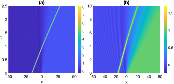
Figure 2: (a) Transmission and (b) trapping of a soliton-RW interaction. Initial data is given in (4.37) with $c=1,\varepsilon=1$ $x_{0}=-15$ and initial amplitude: (a) $A_{0}=8$ and (b) $A_{0}=1.62$.

The first question we address is whether a soliton will or will not become trapped. Broadly speaking, we initially place a soliton mode to one side of the jump (1.6) and examine whether the soliton completely propagates through the resulting RW or DSW mean field in finite time. If the soliton can not travel fast enough to escape the RW or DSW, we call this a trapped or an embedded soliton. Examples are shown in the right panels of Figure 1. When a soliton completely passes through one of the step-induced mean fields, this is called a transmitted or tunneling soliton. Examples are shown in the left panels of Figure 1. In general, transmitted modes correspond to large amplitude initial states. Whether or not a soliton becomes trapped depends on its initial data, e.g. its initial position and amplitude.

A typical case of soliton trapping and tunneling with a RW is shown in Fig. 2. The initial condition is Eq. (1.6) with step up BCs. A relatively large amplitude solitary wave placed to the left of the jump will pass through the ramp region and reach the upper plateau region. On the other hand, a small amplitude soliton will never exit the ramp region of the RW in finite time. As shown below, the precise condition for a soliton tunneling through a RW is that the soliton amplitude be at least twice the step height, i.e. $A_{0}>2c^{2}$.

Next, typical soliton interactions with a DSW are presented in Fig. 3. Here, the initial state is Eq. (1.6) with step down BCs. Any soliton initially placed to the left of the jump will tunnel through the DSW. On the other hand, a soliton with small amplitude placed to the right of the jump may become trapped in the DSW region. As shown below, a soliton in the latter case will become trapped if its initial amplitude is strictly less than twice the step height, i.e. $0<A_{0}<2c^{2}$.

We note that the oscillations in Figure 2 for soliton-RW interaction are a result of the sharp, step-like initial transition that has been approximated by a tanh function for accurate numerical simulations. These oscillations give rise to higher order effects on the soliton-mean field interaction problem hence are not considered in our asymptotic analysis. The oscillation amplitude decays with increasing $t$ and its largest value is inversely proportional to the initial step width. In contrast, the large amplitude DSW oscillations in Fig. 3 persist as $t$ increases.

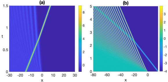
Figure 3: (a) Transmission and (b) trapping of a soliton-DSW. Initial data is given in (4.37) with parameters: (a) $x_{0}=-15,A_{0}=8,c=1,\varepsilon=1$ and (b) $x_{0}=15,A_{0}=4.5,c=2,\varepsilon=1$.

The remainder of this work is divided into three parts where the soliton-mean field interaction is treated using different techniques: Sec. 2, soliton perturbation theory; Sec. 3, Whitham modulation theory; Sec. 4, inverse scattering transform. Within each section, a comparison between analytical predictions and direct numerics is given. The perturbative approach is found to accurately describe the soliton dynamics in the small dispersive and relatively large amplitude limits. The modulation theory approach is shown to provide an accurate description of the solution dynamics when a single phase (soliton-RW) or two-phase (soliton-DSW) ansatz is taken, both interpreted within the context of periodic spectral theory. The IST method is found to yield an exact formula for the solutions as well as a spectral description of the soliton-RW and soliton-DSW interactions. It is here that the notions of proper and pseudo solitons arise. In the case of transmitted solitons, a direct connection between the asymptotic (soliton perturbation and modulation theories) and exact (IST) approach is found in the small dispersion limit. We conclude in Sec. 5.

2 Soliton Perturbation Theory

In this section, we present a simple perturbative approach to approximating the dynamics of a soliton as it passes through a RW or DSW. The general perturbation theory for slowly varying solitary waves was originally introduced in [77] via multiple-scale expansions, providing a detailed description of solitary wave behavior under weak perturbations/slowly varying coefficients. Here we apply a simpler, formal approach that directly yields the leading order terms describing the soliton’s variations due to its interaction with the slowly varying mean field. This setting yields approximate results for the soliton-RW interaction that compare well with other, more sophisticated approaches described in the subsequent sections. The interaction with the rapidly oscillating mean field in a DSW is more complicated, but the direct perturbative approach provides some useful insights in this case as well.

The method assumes: (a) the solution can be expressed as the linear combination of a soliton plus a step-induced wave; (b) the soliton maintains a hyperbolic secant profile (albeit with slowly varying parameters), and (c) the RW or DSW portion of the solution does not depend on the soliton. The above assumptions are quite intuitive and, as we show later, this perturbation theory gives good agreement with the exact solution in the weak dispersion and large amplitude limits, where the soliton profile is narrow relative to the variation in the mean field. Below, we give a general framework that holds for either step up or step down boundary conditions. In the case of step up boundary conditions, we obtain an explicit analytical approximation of the soliton dynamics, whereas for step down, we derive a set of governing differential equations that are solved numerically.

2.1 General Integral Asymptotics Formulation

To begin, we express the solution of Eq. (1.1) as the sum

$$u(x,t)=w(x,t)+v(x,t;w(x,t))\;,$$ (2.1)

where $w(x,t)$ is an approximation of either a RW or DSW and $v(x,t)$ is a solitary mode ansatz with boundary conditions that decay to zero as $|x|\rightarrow\infty$. Notice that the RW/DSW is assumed to be independent of the soliton, but not vice versa. Substituting (2.1) into (1.1) yields

$$v_{t}+6(wv)_{x}+6vv_{x}+\varepsilon^{2}v_{xxx}=-F[w(x,t)]\leavevmode\nobreak\ ,$$ (2.2)

where

$$F[w]\equiv w_{t}+3(w^{2})_{x}+\varepsilon^{2}w_{xxx}\leavevmode\nobreak\ .$$ (2.3)

Note that $F[w]$ is zero if $w$ is a solution of (1.1).

Next, we derive two integral relations from Eq. (2.2). Multiplying (2.2) by $v$ and integrating over $\mathbb{R}$ we obtain

$$\frac{d}{dt}\int_{-\infty}^{\infty}v^{2}dx=6\int_{-\infty}^{\infty}w(v^{2})_{x}\leavevmode\nobreak\ dx-\int_{-\infty}^{\infty}2vF[w]\leavevmode\nobreak\ dx\leavevmode\nobreak\ ,$$ (2.4)

utilizing the decaying BCs of the soliton. This equation describes how the total momentum of the soliton changes with time. The second integral relation we derive is the time evolution of the soliton center of mass (first moment), given by

$$\frac{d}{dt}\left(\frac{\int_{-\infty}^{\infty}xv^{2}dx}{\int_{-\infty}^{\infty}v^{2}dx}\right) =\frac{\frac{d}{dt}\int_{-\infty}^{\infty}xv^{2}dx}{\int_{-\infty}^{\infty}v^{2}dx}-\frac{(\int_{-\infty}^{\infty}xv^{2}dx)\frac{d}{dt}\int_{-\infty}^{\infty}v^{2}dx}{(\int_{-\infty}^{\infty}v^{2}dx)^{2}}\leavevmode\nobreak\ .$$ (2.5)

The first term on the right-hand side of the equation above may be simplified by noting

$$\frac{d}{dt}\int_{-\infty}^{\infty}xv^{2}dx =\int_{-\infty}^{\infty}(12wv(xv)_{x}+4v^{3}-3\varepsilon^{2}v_{x}^{2}+xvF[w])\leavevmode\nobreak\ dx\leavevmode\nobreak\ ,$$ (2.6)

where (2.2) has been applied. Substituting Eqs. (2.4) and (2.6) into (2.5) gives

$$\frac{d}{dt}\left(\frac{\int_{-\infty}^{\infty}xv^{2}dx}{\int_{-\infty}^{\infty}v^{2}dx}\right)= \frac{\int_{-\infty}^{\infty}(12wv(xv)_{x}+4v^{3}-3\varepsilon^{2}v_{x}^{2}+xvF[w])\leavevmode\nobreak\ dx}{\int_{-\infty}^{\infty}v^{2}\leavevmode\nobreak\ dx}$$ (2.7)

$$-\frac{[\int_{-\infty}^{\infty}xv^{2}dx][6\int_{-\infty}^{\infty}w(v^{2})_{x}-\int_{-\infty}^{\infty}2vF[w]\leavevmode\nobreak\ dx]}{[\int_{-\infty}^{\infty}v^{2}\leavevmode\nobreak\ dx]^{2}}\leavevmode\nobreak\ .$$

Equation (2.7) can be further simplified by assuming that $v^{2}(x,t)$ is even-symmetric about the point $x=z(t),$ i.e. $v(x,t)=v(x-z(t))=v(-(x-z(t)))$, hence Eq. (2.7) becomes

$$\frac{dz}{dt}= \frac{\int_{-\infty}^{\infty}12wv(xv)_{x}dx}{\int_{-\infty}^{\infty}v^{2}\leavevmode\nobreak\ dx}+\frac{\int_{-\infty}^{\infty}4v^{3}-3\varepsilon^{2}v_{x}^{2}dx}{\int_{-\infty}^{\infty}v^{2}\leavevmode\nobreak\ dx}+\frac{\int_{-\infty}^{\infty}xvF[w]\leavevmode\nobreak\ dx}{\int_{-\infty}^{\infty}v^{2}\leavevmode\nobreak\ dx}$$ (2.8)

$$-z(t)\frac{\left(\int_{-\infty}^{\infty}6w(v^{2})_{x}-2vF[w]\leavevmode\nobreak\ dx\right)}{\int_{-\infty}^{\infty}v^{2}\leavevmode\nobreak\ dx}\leavevmode\nobreak\ .$$

Motivated by soliton solutions on a constant background (1.2), we look for soliton modes with the secant hyperbolic form

$$v(x,t)=2\kappa^{2}(t){\rm sech}^{2}\left(\frac{\kappa(t)}{\varepsilon}\left[x-z(t)\right]\right)\leavevmode\nobreak\ ,$$ (2.9)

whose parameters $\kappa,z$ depend on time. Notice that Eq. (2.9) solves (1.1) exactly when $w=0$, $\kappa(t)=\kappa_{0}$ and $z(t)=4\kappa_{0}^{2}t+x_{0}$ for $\kappa_{0}>0,x_{0}\in\mathbb{R}$. Substituting the soliton ansatz (2.9) into Eqs. (2.4) and (2.8), we obtain a coupled system of equations that determine $\kappa(t)$ and $z(t)$, amplitude and position, respectively. First, we consider the case when $w$ is a rarefaction wave (step up BC); later, we investigate the DSW case (step down BC).

2.2 Soliton Interaction with Rarefaction Wave

First, we study a soliton-RW interaction with initial condition

$$u(x,0)=c^{2}H(x)+v(x,0;x_{0})\leavevmode\nobreak\ ,$$ (2.10)

for a soliton located to the left or right of the origin at time $t=0$. For $t>0$, a RW forms and connects the left (zero) and right ($+c^{2}$) boundary conditions. The RW that develops is approximated by

$$w(x,t)=\begin{cases}\vspace{0.1 in}0\;,&x\leq 0\\ \vspace{0.15 in}\frac{x}{6t}\;,&0<x\leq 6c^{2}t\\ c^{2}\;,&6c^{2}t<x\end{cases}\leavevmode\nobreak\ ,$$ (2.11)

which is a continuous, global solution of the KdV equation with neglected dispersive term — the approximation is valid away from the points $x=0,6c^{2}t$, namely $F[w]=0$ in Eq. (2.3) away from these points. Thus we will neglect the small, $\mathcal{O}(\varepsilon^{2})$ terms in $\int vF[w]dx$. Near the edges of the RW (2.11) the KdV dispersive term must be taken into account and the weak discontinuities at $x=0,6c^{2}t$ are smoothed. Such higher order regularisation can be achieved, for example, by matched asymptotic methods [40]. Small amplitude oscillations at the left edge of the RW decay according to the typical linear dispersive, long-time estimate $\mathcal{O}(t^{-1/2})$ and the right edge decays exponentially to $c^{2}$. The linear middle region $0<x\leq 6c^{2}t$ of the RW (2.11) is referred to as the ramp region below. Having an explicit and simple approximation formula for the RW allows us to derive a complete characterization of the soliton-RW interaction.

2.2.1 Soliton-Rarefaction Wave Dynamics

The case of the soliton with amplitude $a_{0}\equiv 2\kappa_{0}^{2}$, placed initially to the right of the step ($x_{0}>0$) is rather uninteresting since it moves away from the ramp; so we do not consider it in much detail. Through Galilean invariance, the approximate solution is found to be

$$u(x,t)=w(x,t)+2\kappa_{0}^{2}\leavevmode\nobreak\ \text{sech}^{2}\left(\frac{\kappa_{0}}{\varepsilon}\left[x-(4\kappa_{0}^{2}+6c^{2})t-x_{0}\right]\right)\leavevmode\nobreak\ ,$$ (2.12)

where $\kappa_{0},x_{0}>0$ and the RW is described by (2.11). There is no trapping whatsoever since the soliton is moving faster than the rarefaction ramp.

Now consider a soliton initially placed to the left of the jump ($x_{0}<0$). To obtain a description of the slowly varying soliton (2.9) on the ramp portion of the rarefaction wave, we employ the integral relations (2.4) and (2.8). To begin, rewrite (2.4) as

$$\frac{d}{dt}\int_{-\infty}^{\infty}v^{2}dx=-6\int_{-\infty}^{\infty}w_{x}v^{2}dx\leavevmode\nobreak\ ,$$ (2.13)

and (2.8) as

$$\frac{dz}{dt}=\frac{-\int_{-\infty}^{\infty}12xv(wv)_{x}dx}{\int_{-\infty}^{\infty}v^{2}dx}+\frac{\int_{-\infty}^{\infty}(4v^{3}-3\varepsilon^{2}v_{x}^{2})dx}{\int_{-\infty}^{\infty}v^{2}dx}+z(t)\frac{6\int_{-\infty}^{\infty}w(v^{2})_{x}dx}{\int_{-\infty}^{\infty}v^{2}dx}\leavevmode\nobreak\ ,$$ (2.14)

neglecting $\mathcal{O}(\varepsilon^{2})$ terms as explained above. The soliton in (2.9) propagates with constant positive velocity until it encounters the bottom of the rarefaction ramp at the origin. The time at which the soliton peak reaches the origin is $t=T_{1}$ where

$$T_{1}=-\frac{x_{0}}{4\kappa_{0}^{2}}>0\,.$$ (2.15)

Substituting the RW solution (2.11) into (2.13) yields

$$\frac{d}{dt}\int_{-\infty}^{\infty}v^{2}dx=-\frac{1}{t}\int_{0}^{6c^{2}t}v^{2}dx\leavevmode\nobreak\ .$$ (2.16)

To get a tractable solution, we extend the domain of integration for the second integral to $\mathbb{R}.$ Errors in this approximation occur at the exponentially small tail portion of the soliton, especially when the soliton maximum is near the edges of the ramp region. Then the solution of (2.16) is approximately

$$\int_{-\infty}^{\infty}v^{2}(x,t)dx=\frac{T_{1}}{t}\int_{-\infty}^{\infty}v^{2}(x,T_{1})dx\leavevmode\nobreak\ .$$ (2.17)

Below, we find this approximation improves as $\varepsilon\rightarrow 0$ or $\kappa\rightarrow\infty$ for fixed $x_{0}$ and final time $t$, which corresponds to a narrow soliton width in (2.9) and is consistent with the asymptotic ordering (1.5). Substituting the soliton ansatz (2.9) into Eq. (2.17) and rearranging yields a simple formula

$$\kappa(t)=\kappa_{0}\left(\frac{T_{1}}{t}\right)^{1/3}\leavevmode\nobreak\ ,$$ (2.18)

where $\kappa_{0}>0$ defines the incoming soliton amplitude $a_{0}=2\kappa_{0}^{2}$. This means that the soliton amplitude on the rarefaction ramp decreases as $t$ increases:

$$a(t)=2\kappa^{2}(t)=2\kappa_{0}^{2}\left(\frac{T_{1}}{t}\right)^{2/3},$$ (2.19)

where $t\geq T_{1}>0$. Next, the soliton position while on the linear ramp is computed from (2.14). Again, using the soliton ansatz over the linear portion of the RW gives

$$\frac{dz}{dt}=4\kappa^{2}(t)+\frac{z(t)}{t}\;,$$ (2.20)

whose solution for $z(T_{1})=0$ and $\kappa(t)$ given by (2.18) is

$$z(t)=6\kappa_{0}^{2}t\left[1-\left(\frac{T_{1}}{t}\right)^{2/3}\right].$$ (2.21)

Equation (2.20) tells us that the soliton speed is proportional to the amplitude of the soliton plus the RW solution value at the soliton peak. Note that this equation is not valid for $t<T_{1}.$

The soliton dynamics are now broken down into three regions: (I) soliton traveling on zero background, left of the ramp, where $w(x,t)=0$; (II) soliton propagating on the linear ramp, where $w(x,t)=\frac{x}{6t}$; (III) soliton propagating to the right of the ramp, where $w(x,t)=c^{2}.$ To match these three regions, continuity of $\kappa(t)$ and $z(t)$ is assumed.

Region I: $0\leq t<T_{1},\leavevmode\nobreak\ z(t)<0$

For step-up initial condition (2.10), the soliton is initially placed to the left of the origin at $x=x_{0}<0$. The soliton given in (2.9) travels with constant velocity $4\kappa_{0}^{2}$ a distance $-x_{0}$ until it reaches the bottom of the ramp at $t=T_{1}$. In this time interval the global solution is approximately

$$u(x,t)=\leavevmode\nobreak\ w(x,t)+2\kappa_{0}^{2}\leavevmode\nobreak\ {\rm sech}^{2}\left(\frac{\kappa_{0}}{\varepsilon}\left[x-z(t)\right]\right)\leavevmode\nobreak\ ,$$ (2.22)

$$z(t)=4\kappa_{0}^{2}t+x_{0}\leavevmode\nobreak\ ,$$

where $w(x,t)$ is given by (2.11).

Region II: $T_{1}\leq t<T_{2},\leavevmode\nobreak\ 0<z(t)<6c^{2}t$

The soliton enters the ramp region at time $t=T_{1}$; the bottom of the ramp is located at the origin. The precise moment the soliton reaches the top of the ramp, if it does, is $t=T_{2}$, to be determined. The results in Eqs. (2.18) and (2.21) are used to describe the soliton in this region. The approximate global solution in this time interval is

$$u(x,t)= \leavevmode\nobreak\ w(x,t)+2\kappa_{0}^{2}\left(\frac{T_{1}}{t}\right)^{2/3}{\rm sech}^{2}\left(\frac{\kappa_{0}}{\varepsilon}\left(\frac{T_{1}}{t}\right)^{1/3}\left[x-z(t)\right]\right)\;,$$ (2.23)

$$z(t)=6\kappa_{0}^{2}t\left[1-\left(\frac{T_{1}}{t}\right)^{2/3}\right]\leavevmode\nobreak\ .$$ (2.24)

The soliton tunnels through the RW if it reaches the point $x=6c^{2}t$ i.e. the top of the ramp. Otherwise, the soliton becomes trapped within the RW. For soliton tunneling to occur there must exist a finite time $t=T_{2}>T_{1}$ such that $z(T_{2})=6c^{2}T_{2}$. Using (2.24), we find this condition is met at

$$T_{2}=T_{1}\left(\frac{\kappa_{0}^{2}}{\kappa_{0}^{2}-c^{2}}\right)^{3/2}\leavevmode\nobreak\ .$$ (2.25)

Notice this formula admits real and positive values for $T_{2}$ only when the tunneling condition $\kappa_{0}>c$ is satisfied. The tunneling condition says that only solitons with initial amplitude $2c^{2}$ (twice as large as the step height) will make it to the top of the RW ramp. Otherwise, when $\kappa_{0}\leq c$ this perturbation theory predicts that the soliton will never reach the top in finite time and instead it becomes trapped on the ramp and the approximate solution continues to be described by (2.23) and (2.24) for all $t>T_{1}$. In this case, the soliton amplitude decays algebraically $\propto t^{-2/3}$.

In the case of tunneling, the soliton peak reaches the top of the ramp at

$$z(T_{2})=\frac{6c^{2}\kappa_{0}^{3}T_{1}}{(\kappa_{0}^{2}-c^{2})^{3/2}}=-\frac{3c^{2}\kappa_{0}x_{0}}{2(\kappa_{0}^{2}-c^{2})^{3/2}}\leavevmode\nobreak\ .$$ (2.26)

If the soliton reaches the top of the ramp (from $2\kappa^{2}(T_{2})=2\kappa_{0}^{2}(T_{1}/T_{2})^{2/3}$) we see that it has an amplitude parameter of $\kappa(T_{2})=(\kappa_{0}^{2}-c^{2})^{1/2}$ which means

$$\kappa^{2}(T_{2})=\kappa_{+}^{2}\equiv\kappa_{0}^{2}-c^{2}>0,$$ (2.27)

or, equivalently, $a(T_{2})=2\kappa^{2}(T_{2})>0$, i.e. the existence of $T_{2}>0$ is equivalent to the condition that the amplitude $a(T_{2})$ of the soliton exiting the ramp is positive. As we shall see, relation (2.27) agrees exactly with the Whitham and IST results in Secs. 3.2.3 and 4.1.2, respectively.

Region III: $T_{2}<t,\leavevmode\nobreak\ 6c^{2}t<z(t)$

Only the tunneling soliton, with $\kappa_{0}>c$, reaches this region at the top of the rarefaction ramp. At this point, the soliton is traveling on a constant background and will now travel with constant velocity and amplitude. The approximate solution here is

$$u(x,t)=w(x,t)+2\kappa_{+}^{2}\leavevmode\nobreak\ {\rm sech}^{2}\left(\frac{\kappa_{+}}{\varepsilon}\left[x-z(t)\right]\right)\leavevmode\nobreak\ ,$$ (2.28)

$$z(t)=\left(6c^{2}+4\kappa_{+}^{2}\right)\left(t-T_{2}\right)+z(T_{2})=(6c^{2}+4\kappa_{+}^{2})t+x_{s}^{+}\leavevmode\nobreak\ ,$$ (2.29)

where $\kappa_{+}>0$ is defined in (2.27), and $z(T_{2})$ in (2.26). The term $x_{s}^{+}=z(T_{2})-\left(6c^{2}+4\kappa_{0}^{2}\right)T_{2}$ can be expressed as

$$x_{s}^{+}=\frac{\kappa_{0}x_{0}}{\kappa_{+}}=\frac{x_{0}}{\sqrt{1-\left(\frac{c}{\kappa_{0}}\right)^{2}}}\leavevmode\nobreak\ ,$$ (2.30)

which is less than than $x_{0}$ since $x_{0}<0$. The total phase shift $\Delta\equiv x_{s}^{+}-x_{0}$ is a negative quantity indicating delay or retardation due to the rarefaction ramp.

2.2.2 Comparison with Numerics

In this section, the soliton perturbation theory results are compared with numerical simulations of the KdV equation (1.1). We also present here a comparison with relevant IST and Whitham theory predictions to have an early idea on how the three main analysis methods in this review compare.

Consider the initial condition in (2.10) with step up BCs, $\kappa_{0}>c$, and $x_{0}<0.$ The depiction of a typical soliton transmission through a RW is shown in Figs. 1(a) and 2(a). The soliton travels with velocity $4\kappa_{0}^{2}$ until it reaches the bottom of the ramp. As the soliton travels up the ramp, its amplitude decreases continuously from $2\kappa_{0}^{2}$ to $2\kappa_{+}^{2}=2(\kappa_{0}^{2}-c^{2})$. As this occurs, the velocity of the soliton increases from $4\kappa_{0}^{2}$ to $4\kappa_{+}^{2}+6c^{2}=4\kappa_{0}^{2}+2c^{2}$. To the right of the ramp, the solution is described by (2.28). Note that the integral asymptotic results in this section are identical to the results from Whitham modulation theory presented in Sec. 3.2.3. Several transmitted soliton profiles are shown in Fig. 4 for different values of $\varepsilon$. The IST (see Sec. 4) and numerical results are found to be indistinguishable, while the asymptotic approximations improve as $\varepsilon$ decreases. Note that the soliton perturbation, Whitham, and the small dispersion IST approaches give the same asymptotic description of the soliton.

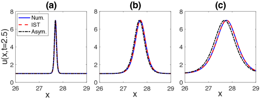
Figure 4: Soliton (post transmission) portion of the solution for (a) $\varepsilon=1/10$, (b) $\varepsilon=1/2$, and (c) $\varepsilon=1$. Shown are numerical, IST, and asymptotic (soliton perturbation and Whitham theories) results. Initial data is given in (4.37) with parameters: $x_{0}=-15,\kappa_{0}=2,c=1$.

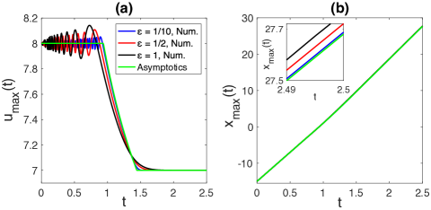
Figure 5: Comparison of (a) amplitude and (b) position corresponding to a transmitted soliton through RW at different values of $\varepsilon$. Initial data is given in (4.37) with parameters: $x_{0}=-15,\kappa_{0}=2,c=1$.

While the soliton is traveling up the ramp, the asymptotic approximation in Eqs. (2.23) and (2.24), or equivalently (3.37) and (3.38), analytically describes the soliton motion. Define $u_{\max}(t)\equiv\max_{x}u(x,t)$, which corresponds to the soliton peak, located at the point $x_{\max}(t)$. The amplitude and position of the soliton peak are numerically computed and displayed in Fig. 5 for fixed $\kappa_{0}$. Note that the amplitude shown in Fig. 5(a) consists of the soliton plus the RW. Initially, the amplitude oscillates due to the small dispersive undulations at the bottom of the ramp (see Fig. 2, $x<0$). Next, the amplitude monotonically decreases until the soliton reaches the top of the ramp, at which point the amplitude is $u_{\max}(t)=c^{2}+2(\kappa_{+})^{2}=2\kappa_{0}^{2}-c^{2}.$ What is apparent from Fig. 5(a) is that the solution behavior is approaching the asymptotic predictions as $\varepsilon\rightarrow 0$. Furthermore, from Fig. 5(b) it is seen that even though the difference between soliton position for different values of $\varepsilon$ is rather small, it too is approaching the asymptotic prediction in the small dispersion limit. It is striking how accurate the asymptotic results are, even when $\varepsilon=\mathcal{O}(1)$. This is because the asymptotic ordering in (1.5) is well-maintained when $|x_{0}|\gg\varepsilon/\kappa_{0}$.

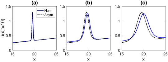
Figure 6: Trapped soliton portion of the solution for (a) $\varepsilon=1/10$, (b) $\varepsilon=1/2$, and (c) $\varepsilon=1$. Shown are numerical and asymptotic results. Initial data is given in (4.37) with parameters: $x_{0}=-15,\kappa_{0}=0.9,c=1$.

In the case of soliton trapping, soliton perturbation theory continues to describe the soliton evolution. Indeed, comparing the asymptotic predictions with the numerical results in Fig. 6 shows excellent agreement as $\varepsilon\rightarrow 0.$ Recall, the asymptotics predict in the $t\rightarrow\infty$ limit that the soliton amplitude $2\kappa(t)^{2}$ decreases like $t^{-2/3}$ and the velocity approaches $6\kappa_{0}^{2}$, which is slower than the top of the ramp that moves with velocity $6c^{2}$. Comparison between the asymptotic approximation and the direct numerics is shown in Fig. 7. The amplitude and position of the solution are found to approach the asymptotic, small dispersion limit. Even when $\varepsilon$ is not so small, the numerically computed soliton amplitude and position exhibit good agreement with that of the asymptotic prediction because the asymptotic ordering (1.5) is maintained.

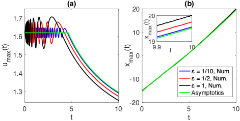
Figure 7: Comparison of (a) amplitude and (b) position of a trapped soliton on top of a RW at different values of $\varepsilon$. Initial data is given in (4.37) with parameters: $x_{0}=-15,\kappa_{0}=0.9,c=1$.

2.3 Soliton Interaction with a Dispersive Shock Wave

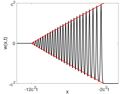
Figure 8: Dispersive mean field $w(x,t)$—a DSW profile obtained from the modulation solution (3.11), (3.16). Included are linear approximations of the DSW envelope.

Let us now consider how a soliton interacts with a DSW. The initial conditions considered are

$$u(x,0)=-c^{2}H(x)+v(x,0;x_{0})\leavevmode\nobreak\ ,$$ (2.31)

where the position of the soliton in (2.9) is taken to the left ($x_{0}<0$) or right ($x_{0}>0$) of the step down. For $t>0,$ a DSW forms and connects the left (zero) and right ($-c^{2}$) boundary conditions. The problem of dispersive regularization of a compressive initial step was first studied by Gurevich and Pitaevskii (GP) in [54] where an asymptotic DSW solution was constructed using Whitham modulation theory [31]. Remarkably, it was shown that the DSW modulation is described by a simple rarefaction wave solution of the Whitham equations. Later, the KdV step problem was studied using rigorous IST, Riemann-Hilbert methods [39], enabling a detailed description of the arising oscillations, which all include the slowly modulated DSW region as the salient, persistent-in-time feature. Here, we take advantage of the results of GP theory combined with the above soliton perturbation approach to describe soliton-DSW interaction.

According to the modulation theory solution [54] (see Section 3.2 for details) the evolution of the step down initial condition can be split into three regions:

$$w(x,t)=\begin{cases}0\;,&\leavevmode\nobreak\ \leavevmode\nobreak\ \leavevmode\nobreak\ \leavevmode\nobreak\ \leavevmode\nobreak\ x<-12c^{2}t\\ w_{D}(x,t)\;,&-12c^{2}t\leq x<-2c^{2}t\\ -c^{2}\;,&\leavevmode\nobreak\ \leavevmode\nobreak\ \leavevmode\nobreak\ \leavevmode\nobreak\ -2c^{2}t\leq x\end{cases}\leavevmode\nobreak\ ,$$ (2.32)

where the interval $(-12c^{2}t,-2c^{2}t)$ is the DSW region with the mean field $w_{D}(x,t)$.

The DSW region is described by a modulated elliptic solution (see (3.11), (3.16)), which is shown in Fig. 8. Despite a rather complicated form of the analytical solution, both the upper and lower DSW envelopes can be reasonably well approximated by the linear functions $\pm(x+12c^{2}t)/(10t)$ for $t>0$. Using this simple heuristic approximation, the soliton-DSW interaction can be viewed as the interaction of a soliton with a descending ramp—the lower DSW envelope—so that we can apply the same soliton perturbation approach as in Section 2.2. As we shall see, this simple decreasing ramp approximation of the DSW mean field gives quantitatively correct predictions for the post-interaction soliton amplitude in the appropriate asymptotic regime as verified by comparison with direct numerical simulations.

As was already noted, an advantage of the soliton perturbation approach is that it does not rely on integrability and hence can be applied to various dispersive systems for which an explicit solitary wave solution is known. This is particularly pertinent to the soliton-DSW interaction as the two other approaches to this problem presented later (2-phase Whitham theory and IST) essentially require the complete integrability of the KdV equation. Indeed, for many non-integrable systems, the edge speeds and the lead solitary wave amplitude necessary for the triangular DSW envelope approximation are available via the DSW fitting method [104, 3].

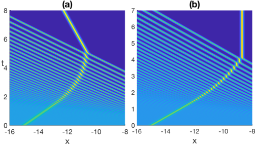
Figure 9: Direct numerical simulations for (a) $\kappa_{0}=3c/5$ (negative exit velocity predicted) and (b) $\kappa_{0}=c/\sqrt{2}$ (zero exit velocity predicted). The initial condition is (4.37) with parameters: $x_{0}=-15,\varepsilon=1/10,c=1$.

2.3.1 Soliton-DSW Dynamics

Motivated by the discussion in the previous Section and in analogy with the rarefaction wave case, we will model the soliton-DSW interaction with a solitary wave ansatz (2.9) on a descending ramp described by the linear approximation of the lower DSW envelope. Specifically, we shall consider

$$w_{D}(x,t)=-\frac{(x+12c^{2}t)}{10t},\leavevmode\nobreak\ \leavevmode\nobreak\ t>0,$$ (2.33)

as the mean field, active in the DSW region, in the calculation of the integral relations (2.4) and (2.8). The motivation lies in the observation that a soliton tunnels through a DSW, see Fig. 9. There are two alternating types of soliton evolution here: propagation down a ramp-like region (approximated by (2.33)), interspersed by nearly instantaneous phase shifts forward due to nonlinear interaction with individual DSW oscillations. The soliton perturbation approach used here only accounts for the average, slow dynamics of the soliton-ramp propagation as in the previous case of the interaction with the rarefaction ramp. Note, however, a key difference is that (2.32), unlike the rarefaction wave (2.11), is not an approximate solution of the KdV equation (1.1).

Consider solitons of the form (2.9) in relations (2.4) and (2.8). If we assume a narrow soliton width, i.e. $\kappa(t)/\varepsilon\gg 1$, then the the soliton-DSW interaction is local, i.e. the solitary wave can be effectively considered as a particle that has nontrivial interaction with only one region of $w$ in Eq. (2.32) at a time. Hence, the integrals in these equations are evaluated over $\mathbb{R}$ for a narrow soliton located in one of the three regions. In the DSW region, these relations yield the linear coupled system

$$\frac{d\kappa}{dt} =-\frac{2z+9c^{2}t}{25\kappa t^{2}}+\frac{\kappa}{5t},$$ (2.34)

$$\frac{dz}{dt} =-\frac{3(z+12c^{2}t)}{5t}+4\kappa^{2},$$ (2.35)

in the small dispersion limit. Note: to obtain Eq. (2.35), we additionally assume that the soliton has a large amplitude ($\kappa\gg 1$) so that the integrals in (2.8) involving $F[w]$, which are $O(\kappa^{-2})$, are neglected in comparison with the other integrals. Also note: to see the linearity, multiply (2.34) by $\kappa$. This approach is simple and yields explicit dynamical equations. As we shall see, it correctly predicts the amplitude via $\kappa(t)$, even for moderate amplitudes, despite the formal large amplitude assumption used in the derivation of (2.34), (2.35). However, as highlighted below, it fails to account for the nonlinear phase shift between the soliton and the local oscillations in the DSW. A correction to account for the phase shifts is necessary to accurately describe the soliton position within the DSW. This would require a significant modification of the linear ramp approximation of the DSW mean field, which would compromise the simplicity of the direct soliton perturbation approach. Instead, in Sec. 3.3, 2-phase Whitham modulation theory, which is based on the integrable theory of KdV, will be used to correctly predict the soliton position within the DSW region. An alternative approach to handle soliton propagation through a DSW involves soliton gas theory [29] and yields, in the end, the same description [105] as that described in Sec. 3.3.

Within the soliton perturbation approach, the soliton-DSW interaction spatial domain can be split into three parts: (I) to the left of the DSW region, where $w=0$; (II) within the DSW region, where $w=w_{D}$; and (III) to the right of the DSW region, where $w=-c^{2}$. The soliton to be considered is initially placed either to the left or right of the jump. When placed to the left of the step, the soliton always tunnels through the DSW. If the soliton is initially placed to the right of the step, then two scenarios are possible. If the soliton’s amplitude is sufficiently small, then it will become trapped inside the DSW. Conversely, sufficiently large amplitude solitons never enter the DSW region when initially placed to the right of the jump. The dynamics within each resion are described in more detail below.

Region I: $z(t)<-12c^{2}t$

A soliton with amplitude $2\kappa_{0}^{2}$ is initially centered at $x=x_{0}<0$ and travels with constant positive velocity $4\kappa^{2}_{0}$ until it’s peak reaches the left edge of the DSW. This edge of the DSW moves with constant negative velocity $-12c^{2}$, so the time at which the soliton peak meets the DSW is $4\kappa_{0}^{2}t+x_{0}=-12c^{2}t$, or

$$T_{1}=-\frac{x_{0}}{4\kappa_{0}^{2}+12c^{2}}>0\leavevmode\nobreak\ .$$ (2.36)

When the soliton is in Region I, the solution is approximated by

$$u(x,t)= w(x,t)+2\kappa_{0}^{2}\leavevmode\nobreak\ {\rm sech}^{2}\left(\frac{\kappa_{0}}{\varepsilon}\left[x-z(t)\right]\right)\;,$$ (2.37)

$$z(t)=4\kappa_{0}^{2}t+x_{0}\leavevmode\nobreak\ ,$$

where $w(x,t)$ is given in Eq. (2.32). We point out that this region occurs only when a soliton is initially placed to the left of the jump. A soliton initially placed to the right of the jump will never be able to tunnel all the way backward through the DSW.

Region II: $-12c^{2}t<z(t)<-2c^{2}t$

In this region, the soliton is interacting with the DSW. Depending on the initial position and amplitude, the soliton can enter the DSW region from either direction. The IST results from Sec. 4 tell us that a soliton that starts to the left of a jump ($x_{0}<0$) moves in the positive direction, hence it will tunnel through the DSW, which moves to the left in the chosen reference frame specified by the initial jump $-c^{2}H(x)$. On the other hand, for $x_{0}>0$, sufficiently small amplitude solitons with $\kappa_{0}<c$ will eventually be trapped within the DSW. If on the other hand, $\kappa_{0}\geq c$, then the soliton’s speed is larger than the DSW’s right edge speed, hence it will never interact the DSW region.

For both cases, the soliton perturbation theory model in (2.34)–(2.35) provides useful predictions for the dynamics of soliton-DSW interaction. In the case of large, transmitting ($x_{0}<0$) solitons, the local, soliton-DSW oscillatory phase shift is small, so the dynamics are effectively described by the dynamical system (2.34), (2.35). If, on the other hand, the soliton amplitude is suitably small, then the soliton interacts with the DSW’s oscillatory region for an extended period of time. As such, it experiences many phase shifts forward that can appreciably accumulate. This model does not incorporate the effect of these phase shifts. A more sophisticated theory is needed (see Sec. 3.3). Regardless, for the initial soliton amplitudes examined, soliton perturbation theory provides a good, quantitative prediction for the amplitude of the transmitted soliton; see Fig. 10.

In the case of solitons initialized to the right of the jump ($x_{0}>0$), the interesting case is that of trapping. The asymptotic model predicts a localized solitary wave that gradually loses all its amplitude. While numerics appear to suggest a loss of amplitude, the form of the solitary wave no longer resembles the hyperbolic secant function in (2.9). Rather, the solution appears to take the form of a DSW modulated by a depression or dark envelope type structure (see Fig. 1(d)). This is different from the perturbed soliton form assumed in (2.1) and is not captured by the simple soliton perturbation theory developed here.

Region III: $-2c^{2}t<z(t)$

When the soliton propagates to the right of the DSW region, it is effectively on the constant background $-c^{2}$. When a soliton transmits through the DSW and $x_{0}<0$, the approximate solution is

$$x_{0}<0:\leavevmode\nobreak\ \leavevmode\nobreak\ \leavevmode\nobreak\ \leavevmode\nobreak\ \leavevmode\nobreak\ \leavevmode\nobreak\ \leavevmode\nobreak\ u(x,t)=w(x,t)+2(\kappa_{-})^{2}\leavevmode\nobreak\ {\rm sech}^{2}\left(\frac{\kappa_{-}}{\varepsilon}\left[x-z(t)\right]\right)\;,$$ (2.38)

$$\leavevmode\nobreak\ \leavevmode\nobreak\ \leavevmode\nobreak\ \leavevmode\nobreak\ \leavevmode\nobreak\ \leavevmode\nobreak\ z(t)=(4(\kappa_{-})^{2}-6c^{2})t+x_{s}^{-}\leavevmode\nobreak\ ,$$

where $\kappa_{-}$ is the soliton amplitude parameter upon exiting the DSW region. In this soliton perturbation theory, we do not have an analytical formula for $\kappa_{-}$; instead, we must numerically compute it by integrating (2.34), (2.35). One can see from Fig. 10 that the model here agrees with direct numerical simulations of soliton-DSW tunneling. We note that the exact, analytical result $\kappa_{-}=\sqrt{\kappa_{0}^{2}+c^{2}}$ is available through the IST and Whitham theory approaches described later. The phase shift $\Delta x_{-}=x_{s}^{-}-x_{0}$ is not captured by the simple soliton perturbation approach employed here; we will compute it using Whitham theory in Section 3.3.1 and using IST asymptotics.

If, on the other hand, the soliton starts to the right of the jump, $x_{0}>0$, two outcomes are possible: $\kappa_{0}\geq c$ and the soliton never reaches the DSW; or $\kappa_{0}<c$ and the soliton will eventually embed itself within the DSW. The first case is trivial as the approximate solution is just a superposition of a well-separated soliton and a DSW. The second case is not tractable using the soliton perturbation approach presented here.

Here, the initial soliton amplitude is expressed in terms of $\kappa_{0}$ in order to be consistent with the IST convention below. The solution in this region is described by

$$x_{0}>0:\leavevmode\nobreak\ \leavevmode\nobreak\ \leavevmode\nobreak\ \leavevmode\nobreak\ \leavevmode\nobreak\ \leavevmode\nobreak\ \leavevmode\nobreak\ u(x,t)=w(x,t)+2\kappa_{0}^{2}\leavevmode\nobreak\ {\rm sech}^{2}\left(\frac{\kappa_{0}}{\varepsilon}\left[x-z(t)\right]\right)\;,$$ (2.39)

$$\leavevmode\nobreak\ \leavevmode\nobreak\ \leavevmode\nobreak\ \leavevmode\nobreak\ \leavevmode\nobreak\ \leavevmode\nobreak\ z(t)=(4\kappa_{0}^{2}-6c^{2})t+x_{0}.$$

for short times. This approximation holds for all $t>0$ when $\kappa_{0}>c$ since the soliton velocity will always be larger than the rightmost DSW edge velocity, i.e. $4\kappa_{0}^{2}-6c^{2}>-2c^{2}$. In the trapping case, when $-2c^{2}t=(4\kappa_{0}^{2}-6c^{2})t+x_{0}$, or equivalently at time

$$T_{D}=-\frac{x_{0}}{4(\kappa_{0}^{2}-c^{2})}\leavevmode\nobreak\ ,$$ (2.40)

the soliton reaches the DSW’s rightmost edge and embeds itself inside the DSW region (Region II).

2.3.2 Comparison with Numerics

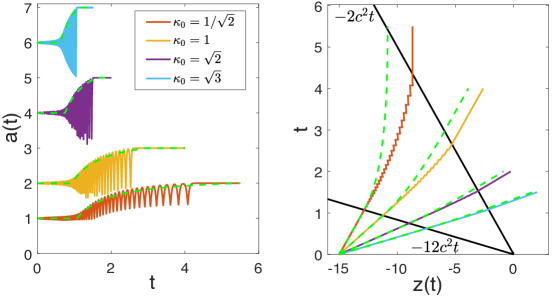
Figure 10: Comparison of soliton amplitude $a(t)$ and position $z(t)$ for direct numerical simulations (solid curves) and asymptotic predictions of soliton perturbation theory (dashed curves). The initial condition used is (4.37) with parameters: $x_{0}=-15,\varepsilon=1/10,c=1$.

A summary of typical results produced by this model is shown in Fig. 10. The predicted soliton amplitude, $a(t)=2\kappa(t)^{2}+w(z(t),t)$, and position, $z(t)$, are shown as functions of time and are compared with direct numerical simulations. The full solution can be reconstructed from the ansatz (2.1). Note that the model predicts the “effective”, average soliton amplitude shown in Fig. 10, left panel, with dashed line, whereas the local, instantaneous amplitude, shown with the solid line, is oscillating due to the interaction of the tunneling soliton with individual oscillations within the DSW. Such oscillations were recently described analytically for the modified KdV equation using rigorous asymptotic theory in [28].

As the soliton passes through the DSW region, its average amplitude increases, while its velocity decreases. Depending on the incoming amplitude, a transmitted soliton can have either negative ($\kappa_{0}<c/\sqrt{2}$), zero ($\kappa_{0}=c/\sqrt{2}$), or positive ($\kappa_{0}>c/\sqrt{2}$) exit velocity.

Interestingly, regardless of the initial amplitude, the system (2.34)–(2.35) does an excellent job of predicting the transmitted soliton amplitude. The errors in the exit amplitudes are less than $O(10^{-6})$ for all cases checked. Moreover, for a large incoming soliton, this system is found to describe its position $z(t)$ well (see Fig. 10, right panel). For smaller values of $\kappa$, the soliton remains inside the DSW region for too long. As stated earlier, nonlinear phase shift interactions between the soliton and the two successive minima of the DSW are required. This effect is not captured by the soliton perturbation model. However, the total phase shift is predicted by modulation theory presented in Section 3.3.

Finally, the trapped soliton case ($x_{0}>0$) is also out of reach of the soliton perturbation method as the hyperbolic secant ansatz (2.9) does not accurately describe the spatial profile of the trapped soliton. A more sophisticated analysis is needed. Such analysis based on the spectral finite-gap modulation theory of the soliton-DSW interaction is presented in Section 3.3.

3 Whitham Modulation Theory

In this section, we study the problem of soliton-RW and soliton-DSW interaction using multiphase Whitham modulation theory developed for the KdV equation in [53]. Whitham theory, originally introduced in [76, 31] for the single-phase case, has been successfully applied to the asymptotic description of dispersive shock waves in the zero dispersion limit [54, 3]. Multiphase Whitham theory has been utilized to describe wavebreaking in the Whitham equations [55], DSW-DSW interaction [73], and admits a thermodynamic limit describing a gas of solitons [74]. Here, we utilize certain degenerate limits of the 1- and 2-phase Whitham modulation equations to asymptotically describe the interaction of a soliton with a RW and a DSW, respectively.

The KdV equation (1.1) admits a family of quasi-periodic or multiphase solutions in the form [57, 58, 59, 56]

$$u(x,t)=F_{N}(\theta_{1}/\varepsilon,\theta_{2}/\varepsilon,\ldots,\theta_{N}/\varepsilon).$$ (3.1a)

The integer $$N\in\{0,1,2,\cdots\} \theta_{j}=k_{j}x-\omega_{j}t+\theta_{0j} j=1,\ldots,N N=0 N F_{N} 2\pi 0<\varepsilon\ll 1 N=1 j^{\rm th} k_{j} \omega_{j} \theta_{0j} j=1,\ldots,N \int_{0}^{2\pi}\cdots\int_{0}^{2\pi}F_{N}(\theta_{1}/\varepsilon,\ldots,\theta_{N}/\varepsilon)\,\mathrm{d\theta_{1}}\cdots\mathrm{d\theta_{N}}/(2\pi)^{N} N N \{\theta_{j}\}_{j=1}^{N}$$ corresponds to the number of nontrivial, independent variables (called phases) , required to describe the solution. The case corresponds to a constant solution. The -phase solution is normalized so that is -periodic in each phase, i.e., rapidly varying for . For example, the case corresponds to the well-known KdV cnoidal traveling wave solution. The phase’s wavenumber , frequency , and phase shift at the origin for and the mean completely determine the -phase solution. The representation of the -phase solution in the form (3.1a) requires use of multidimensional theta functions [59]. Although it obscures the dependence of the solution on the independent phases , an alternative representation that provides practical advantages is the so-called trace formula [60]

$$u(x,t)=\Lambda-2\sum_{j=1}^{N}\mu_{j}(x,t),\quad\Lambda\equiv\sum_{k=1}^{2N+1}\lambda_{k},$$ (3.1b)

where the constants $\lambda_{k}$, $k=1,\ldots,2N+1$ bound the functions $\mu_{j}(x,t)\in[\lambda_{2j-1},\lambda_{2j}]$, $j=1,2,\ldots,N$, which satisfy the Dubrovin system [60]

$$\begin{split}\varepsilon\partial_{x}\mu_{j}&=\frac{2\sigma_{j}R(\mu_{j})}{\prod_{i\neq j}(\mu_{i}-\mu_{j})},\\ \varepsilon\partial_{t}\mu_{j}&=\left(u+2\mu_{j}\right)\frac{4\sigma_{j}R(\mu_{j})}{\prod_{i\neq j}(\mu_{i}-\mu_{j})},\quad R(\lambda)=\sqrt{\prod_{k=1}^{2N+1}(\lambda-\lambda_{k})}.\end{split}$$ (3.2)

The coefficient $\sigma_{j}=\pm 1$ changes sign so that $\mu_{j}(x,t)$ oscillates between its maximum $\lambda_{2j}$ and minimum $\lambda_{2j-1}$. In the form (3.1b), the $2N+1$ constants $\{\lambda_{k}\}_{k=1}^{2N+1}$ and the $N$ initial conditions $\{\mu_{j}(0,0)\}_{j=1}^{N}$ completely determine the $N$-phase solution. These $3N+1$ constants are in one-to-one correspondence with the wavenumbers, frequencies, mean and phase shifts associated with the solution in the form (3.1a) [53].

The above results on multiphase KdV solutions were obtained in the framework called finite-gap spectral theory. Within this theory, the parameters $\lambda_{k}$ in (3.1b), (3.2) are the band edges of the Schrödinger operator

$$\mathcal{L}=\varepsilon^{2}\partial_{xx}+u(x,t)$$ (3.3)

with the potential (3.1). Note that $\mathcal{L}+\lambda$ is also the scattering operator that will be used in (4.1). The real spectral parameter $\lambda\in\mathcal{S}_{N}$ corresponding to $L(\mathbb{R})^{\infty}$ eigenfunctions of (3.3) with $u=F_{N}$ lies in the union of bands

$$\mathcal{S}_{N}=(-\infty,\lambda_{1}]\cup[\lambda_{2},\lambda_{3}]\cup\cdots\cup[\lambda_{2N},\lambda_{2N+1}].$$ (3.4)

Thus, the band edges $\{\lambda_{k}\}_{k=1}^{2N+1}$ parametrize the $N$-phase solution $u$ in (3.1b) (up to the $N$ initial conditions $\mu_{j}(0,0)$, $j=1,\ldots,N$). Finite-gap theory can be regarded as a periodic analogue of IST on the real line that will be used in the next section for the exact description of the soliton-mean field interaction. In what follows, we take advantage of some results from KdV finite-gap theory and apply them to the approximate, modulation description of the soliton-mean interaction.

The $N$-phase KdV-Whitham equations [53]

$$\frac{\partial\lambda_{k}}{\partial t}+v_{k}(\boldsymbol{\lambda})\frac{\partial\lambda_{k}}{\partial x}=0,\quad k=1,\ldots,2N+1,$$ (3.5)

asymptotically describe modulations of $N$-phase solutions (3.1) to the KdV equation (1.1) in the limit $\varepsilon\to 0$ [62, 63, 64, 65]. The characteristic velocities are

$$v_{k}=-6\Lambda+12\lambda_{k}+12\frac{\det\mathrm{Q}(\lambda_{k})}{\det\mathrm{P}(\lambda_{k})},$$ (3.6)

where the $N\times N$ matrices $\mathrm{P}(\lambda_{k})$ and $\mathrm{Q}(\lambda_{k})$ are defined component-wise by elliptic integrals, in the $N=1$ case, or hyperelliptic integrals otherwise

$$\mathrm{P}(\lambda_{k})_{ij}=\int_{\lambda_{2i-1}}^{\lambda_{2i}}\frac{(\lambda_{k}-\mu)\mu^{j-1}}{R(\mu)}\,\mathrm{d}\mu,\quad\mathrm{Q}(\lambda_{k})_{ij}=\int_{\lambda_{2i-1}}^{\lambda_{2i}}\frac{(\lambda_{k}-\mu)\mu^{j-1+\delta_{jN}}}{R(\mu)}\,\mathrm{d}\mu.$$ (3.7)

Note that $v_{k}$ depends on the $2N+1$ modulation variables $\lambda_{k}$, $k=1,\ldots,2N+1$. We highlight a very special property of the KdV-Whitham modulation equations (3.5), which is their diagonal structure. The remarkable fact that the Riemann invariants of the KdV-Whitham system $\{\lambda_{k}\}_{k=1}^{2N+1}$ are precisely the band edges of the finite-gap Schrödinger operator (3.3) was discovered in [53]. The modulation variables and velocities are ordered

$$\lambda_{1}\leq\lambda_{2}\leq\cdots\leq\lambda_{2N+1},\quad v_{1}\leq v_{2}\leq\cdots\leq v_{2N+1}$$ (3.8)

and the modulation equations (3.5) are strictly hyperbolic and genuinely nonlinear [66]. The notion of strict hyperbolicity is defined to be $v_{1}<v_{2}<\cdots<v_{2N+1}$ if and only if $\lambda_{1}<\lambda_{2}<\cdots<\lambda_{2N+1}$. It has been shown that for $N$-phase modulations where $\lambda_{i}\to\lambda_{j}$ with $j=i\pm 1$, then $v_{i}\to v_{j}$ and the remaining modulation variables and velocities correspond to the $N-1$-phase modulation equations [61, 65, 55]. Thus, the modulations of the $N-1$-phase solution described by the $2N-1$ variables $\{\lambda_{k}\}_{k=1}^{2N+1}\setminus\{\lambda_{ij}\equiv\lambda_{i}=\lambda_{j}\}$ completely decouple from and evolve independently of the degenerate phase described by the single, coalesced modulation variable $\lambda_{ij}$. In this section, we identify $\lambda_{ij}$ with a soliton interacting with a RW and a DSW in the degeneration of $1$- and $2$-phase modulations, respectively. We determine the respective characteristic velocities $v_{ij}\equiv v_{i}=v_{j}$ and use the constant Riemann invariant $\lambda_{ij}$ to completely describe the transmission and trapping of a soliton by a RW and a DSW.

We note that, due to the ordering (3.8), all limits of the form $\lambda_{i}\to\lambda_{j}$ are to be understood as one-sided limits: $\lambda_{i}\to\lambda_{i+1}^{-}$ or $\lambda_{i}\to\lambda_{i-1}^{+}$.

While the Whitham velocities $v_{k}$ in (3.6) are generally expressed in terms of complete hyperelliptic integrals, they can be simplified in certain important cases. For the soliton-mean field interaction problem, we will make particular use of the Whitham equations with $N\in\{0,1,2\}$.

Recall that the term mean field is used to describe both RWs and oscillatory DSWs whose mean vary on a much slower spatial scale than the soliton width. As we will see, this is reflected in the structure of the modulation equations that decouple the descriptions of the RW and DSW from soliton propagation. On the other hand, the soliton dynamics will be significantly altered by the presence of the mean field.

3.1 Mean Fields: 0-Phase Modulations

The $N=0$ Whitham equation is

$$\frac{\partial\lambda_{1}}{\partial t}+v_{1}\frac{\partial\lambda_{1}}{\partial x}=0,\quad v_{1}(\lambda_{1})=6\lambda_{1},$$ (3.9a)

which is obtained by simply sending $$\varepsilon\to 0 u\to\lambda_{1} |u_{x}/u|\sim|u_{t}/u|={\cal O}(1) \overline{u}=\lambda_{1}$$ in the KdV equation (1.1) and identifying . Thus, the Hopf equation (3.9a) describes slowly varying , dispersionless dynamics. We identify these dynamics with mean fields and write the dependent variable in the suggestive form so that the 0-phase equation (3.9a) becomes

$$\overline{u}_{t}+6\overline{u}\,\overline{u}_{x}=0,$$ (3.9b)

and describes the modulations of the constant ($0$-phase) solution (3.1a) $u=\overline{u}$ of the KdV equation.

The solutions of (3.9) are simple waves and include the centered rarefaction wave (2.11), which we reproduce here for convenience using the notation $\overline{u}(x,t)$ for the mean field,

$$\frac{x}{t}=6\overline{u}(x,t),\quad 0\leq\overline{u}(x,t)\leq c^{2},\quad\overline{u}(x,t)=\begin{cases}0&x<0\\ c^{2}&x>6c^{2}t\end{cases}.$$ (3.10)

In this case, the spectrum of $\mathcal{L}$ (3.3) consists of the single semi-infinite band $\mathcal{S}_{0}=(-\infty,\lambda_{1}]$ whose band edge is the slowly varying mean $\overline{u}$ depicted in Fig. 11.

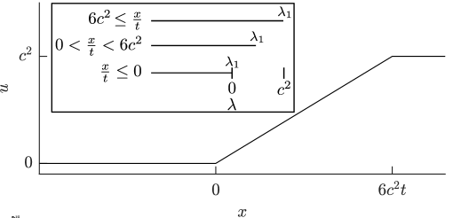
Figure 11: Self-similar RW solution. The inset represents the associated variation of the 0-phase spectrum $\mathcal{S}_{0}$ in the self-similar variable $x/t$.

Any initial condition for the 0-phase modulation equation (3.9) with a decreasing part exhibits gradient catastrophe in finite time. This singularity is regularized by adding another phase to the modulated solution (3.1a). Thus we are led to a 1-phase, i.e., periodic, modulated wave and the $N=1$ Whitham equations.

3.2 Soliton-Mean Field Interaction: 1-Phase Modulations

The $N=1$ Whitham equations describe slow modulations of the periodic cnoidal wave solution, which is expressed in terms of the modulation variables $\boldsymbol{\lambda}=(\lambda_{1},\lambda_{2},\lambda_{3})$ as

$$u(\Theta/\varepsilon,x,t)=\lambda_{1}-\lambda_{2}+\lambda_{3}+2(\lambda_{2}-\lambda_{1})\mathrm{cn}^{2}\left(\frac{K(m)}{\varepsilon\pi}\Theta,m\right),\quad m=\frac{\lambda_{2}-\lambda_{1}}{\lambda_{3}-\lambda_{1}}.$$ (3.11)

The wavenumber and frequency are related to the modulation variables according to

$$\Theta_{x}=k=\frac{\pi\sqrt{\lambda_{3}-\lambda_{1}}}{K(m)},\quad\Theta_{t}=-\omega,\quad V\equiv\frac{\omega}{k}=2(\lambda_{1}+\lambda_{2}+\lambda_{3}).$$ (3.12)

The Whitham velocities can be expressed in terms of complete elliptic integrals

$$\begin{split}v_{1}&=V-4(\lambda_{2}-\lambda_{1})\frac{K(m)}{K(m)-E(m)},\\ v_{2}&=V-4(\lambda_{2}-\lambda_{1})\frac{(1-m)K(m)}{E(m)-(1-m)K(m)},\\ v_{3}&=V+4(\lambda_{3}-\lambda_{2})\frac{K(m)}{E(m)}.\end{split}$$ (3.13)

These expressions were originally obtained in the foundational Whitham paper [76]. The mean and amplitude of the cnoidal solution (3.11) are

$$\overline{u}\equiv\frac{1}{2\pi}\int_{0}^{2\pi}u(\Theta/\varepsilon,x,t)\,\mathrm{d}(\Theta/\varepsilon)=\lambda_{1}+\lambda_{2}-\lambda_{3}+2(\lambda_{3}-\lambda_{1})\frac{E(m)}{K(m)},$$ (3.14)

and

$$a=2(\lambda_{2}-\lambda_{1}),$$ (3.15)

respectively.

The 1-phase Whitham equations serve two purposes for us. First, the centered rarefaction solution with constant $\lambda_{1}=-c^{2}$, $\lambda_{3}=0$, and $\lambda_{2}$ implicitly defined by

$$\frac{x}{t}=v_{2}(-c^{2},\lambda_{2}(x,t),0),\quad-c^{2}\leq\lambda_{2}(x,t)\leq 0,\quad\lambda_{2}(x,t)=\begin{cases}-c^{2}&x<v_{12}(-c^{2},-c^{2},0)t\\ 0&x>v_{23}(-c^{2},0,0)t\end{cases},$$ (3.16)

is the celebrated Gurevich-Pitaevskii modulation solution for a DSW [54]. The DSW, reconstructed from the modulation solution (3.16) in Fig. 12, is an example of a dispersive mean field exhibiting rapid oscillations. The spatiotemporal evolution of the DSW’s 1-phase spectrum $\mathcal{S}_{1}$ according to the GP solution (3.16) is shown in the inset of Fig. 12.

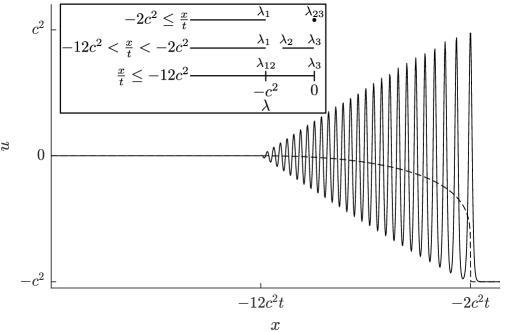
Figure 12: Reconstruction of the KdV DSW (solid) from the self-similar GP modulation solution and its mean $\overline{u}$ (dashed). The inset represents the associated variation of the 1-phase spectrum $\mathcal{S}_{1}$.

The second use of the 1-phase Whitham equations is to describe the interaction of a soliton and a mean field. For both purposes, we need to understand the limiting behavior of the 1-phase equations and the associated spectrum $\mathcal{S}_{1}$ when $\lambda_{2}\to\lambda_{3}=\lambda_{23}$. For the DSW, we also need to consider the limit $\lambda_{2}\to\lambda_{1}=\lambda_{12}$, which we consider first.

3.2.1 Harmonic Limit: Merged 1-Phase Spectrum

When $\lambda_{2}\to\lambda_{1}$, the cnoidal wave (3.11) is a vanishing harmonic wave

$$u(\Theta/\varepsilon,x,t)\sim\lambda_{3}+(\lambda_{2}-\lambda_{1})\cos\left(\Theta/\varepsilon\right),\quad\lambda_{2}\to\lambda_{1},$$ (3.17)

with wavenumber

$$k=2\sqrt{\lambda_{3}-\lambda_{12}}.$$ (3.18)

Passing to the limit in the Whitham velocities (3.13), we have $v_{1}\to v_{2}=v_{12}$ where

$$v_{12}=6(\lambda_{3}-2\lambda_{1}),\quad\lim_{\lambda_{2}\to\lambda_{1}}v_{3}=6\lambda_{3}.$$ (3.19)

The limit $\lambda_{2}\to\lambda_{1}$ results in two modulation equations describing a linear wave on a slowly varying mean (3.17). To see this, we substitute $K=k/\varepsilon$ and $\Omega=\omega/\varepsilon$ from (3.12) and (3.18), $\overline{u}\to\lambda_{3}$ from (3.14) and recognize one characteristic velocity as the group velocity $v_{12}=\Omega^{\prime}(K)=6\overline{u}-3\varepsilon^{2}K^{2}$ of linear traveling wave solutions $\sim e^{i(Kx-\Omega t)}$ to the KdV equation (1.1). The remaining velocity in (3.19) is $v_{3}\to 6\overline{u}$, where $\lambda_{3}=\overline{u}$ coincides with the mean field, 0-phase modulation (3.9). The mean field completely decouples from the linear wave modulation, which is expressed in the spectrum (3.4) as a degenerate point embedded within the semi-infinite band

$${\cal S}_{1}^{(12)}\equiv\lim_{\lambda_{2}\to\lambda_{1}}{\cal S}_{1}=(-\infty,\lambda_{12}]\cup[\lambda_{12},\lambda_{3}]=(-\infty,\lambda_{3}].$$ (3.20)

The superscript ⁽¹²⁾ notation represents the merger of the semi-infinite band $(-\infty,\lambda_{1}]$ with the finite band $[\lambda_{2},\lambda_{3}]$, so that ${\cal S}_{1}^{(12)}$ is the merged 1-phase spectrum. This merging process is depicted in Fig. 13. Modulations of the spectrum $\mathcal{S}_{1}^{(12)}$ have been used to describe the transmission and trapping of a linear wavepacket with a RW in [35].

The DSW spectral evolution shown in Fig. 12 also exhibits spectral merger at the DSW’s harmonic edge when the finite band expands to merge with the semi-infinite band for $x\to-12c^{2}t$.

3.2.2 Soliton Limit: Collapsed 1-Phase Spectrum

When $\lambda_{2}\to\lambda_{3}$, the cnoidal wave (3.11) limits to

$$u(\xi/\varepsilon,x,t)=\lambda_{1}+2(\lambda_{23}-\lambda_{1})\mathrm{sech}^{2}\left(\sqrt{\lambda_{23}-\lambda_{1}}\,\xi/\varepsilon\right),\quad\xi=x-(2\lambda_{1}+4\lambda_{23})t,$$ (3.21)

which corresponds to the soliton solution of the KdV equation (1.1). Note that this limit is singular ($k\to 0$) so that the phase $\Theta$ in (3.11) is undefined and we identify $\xi/\varepsilon$ as the fast variable according to

$$\lim_{\lambda_{2}\to\lambda_{3}}\frac{K(m)}{\varepsilon\pi}\Theta=\frac{\sqrt{\lambda_{23}-\lambda_{1}}\,\xi}{\varepsilon}.$$ (3.22)

The $N=1$ Whitham velocities (3.13) limit to

$$\lim_{\lambda_{2}\to\lambda_{3}}v_{1} =6\lambda_{1},\quad v_{23}=2\lambda_{1}+4\lambda_{23},$$ (3.23)

so that the 1-phase Whitham modulation equations (3.5) become

$$\frac{\partial\lambda_{1}}{\partial t}+6\lambda_{1}\frac{\partial\lambda_{1}}{\partial x} =0,$$ (3.24a)

$$\frac{\partial\lambda_{23}}{\partial t}+(2\lambda_{1}+4\lambda_{23})\frac{\partial\lambda_{23}}{\partial x} =0.$$ (3.24b)

Using (3.14) and (3.15), we can express the Riemann invariants in this limit in terms of the wave mean and amplitude as

$$\lambda_{1}=\overline{u},\quad\lambda_{23}=\frac{a}{2}+\overline{u}.$$ (3.25)

Figure 13: Degeneration pathways for the 1-phase spectrum $\mathcal{S}_{1}$. When $\lambda_{2}\to\lambda_{1}$, the two bands merge into a single, semi-infinite band, the merged spectrum $\mathcal{S}_{1}^{(12)}$. When $\lambda_{2}\to\lambda_{3}$, the finite band collapses into a single point, the collapsed spectrum $\mathcal{S}_{1}^{(23)}$.

Consequently, we can identify the 1-phase modulation equations (3.24) in the limit $\lambda_{2}\to\lambda_{3}$ with the 0-phase mean field modulation equation (3.24a) for $\lambda_{1}$ (cf. eq. (3.9)) and the equation (3.24b) for $\lambda_{23}$ represents modulation of the soliton amplitude. The double Whitham velocity $v_{23}$ is the soliton velocity

$$v_{23}=s(a,\overline{u})=6\overline{u}+2a,$$ (3.26)

and the soliton trajectory $x_{s}(t)$ is the characteristic

$$\frac{\mathrm{d}x_{s}}{\mathrm{d}t}=s,\quad x_{s}(0)=x_{0}.$$ (3.27)

These soliton-mean field modulations equations were also obtained using multiple scale perturbation theory in [77].

The mean field modulation fully decouples from the soliton amplitude modulation, which manifests in the degenerate spectrum

$${\cal S}_{1}^{(23)}\equiv\lim_{\lambda_{2}\to\lambda_{3}}{\cal S}_{1}=(-\infty,\lambda_{1}]\cup\{\lambda_{23}\}$$ (3.28)

consisting of the semi-infinite band of the 0-phase spectrum and the point spectrum or eigenvalue $\lambda_{23}$. In fact, the spectrum ${\cal S}_{1}^{(23)}$ corresponds to the classical 1-soliton solution on a constant background in the framework of IST, which we will describe in detail in Sec. 4. Here, the superscript ⁽²³⁾ corresponds to the collapse of the second band $[\lambda_{2},\lambda_{3}]$ in the 1-phase spectrum to a point and we refer to ${\cal S}_{1}^{(23)}$ as the collapsed 1-phase spectrum. An example of this is shown in Fig. 13.

The DSW spectral evolution shown in Fig. 12 also exhibits spectral collapse when the finite band collapses to a point at $x\geq-2c^{2}t$.

3.2.3 Soliton-RW Interaction

We are now in a position to approximate the interaction of a soliton and a slowly varying mean field by modulations of the collapsed 1-phase spectrum ${\cal S}_{1}^{(23)}$ (3.28) whose band edge $\lambda_{1}$ and point spectrum $\lambda_{23}$ evolve according to the degenerate 1-phase Whitham equations (3.24). We focus on the soliton-RW interaction resulting from step-up initial data (1.6) ($+$ sign) and approximate the initial soliton $v(x,0;x_{0})$ according to a spatially translated, modulated soliton (3.21)

$$u(x,0)=\lambda_{1}+2(\lambda_{23}-\lambda_{1})\mathrm{sech}^{2}\left(\sqrt{\lambda_{23}-\lambda_{1}}(x-x_{0})/\varepsilon\right).$$ (3.29)

The step is represented by the initial mean field

$$\lambda_{1}(x,0)=\begin{cases}0&x<0\\ c^{2}&x>0\end{cases},$$ (3.30)

which, when evolved according to (3.24a), is the RW solution (cf. (3.10))

$$\lambda_{1}(x,t)=\begin{cases}0&x<0\\[8.53581pt] \displaystyle\frac{x}{6t}&0<x<6c^{2}t\\[8.53581pt] c^{2}&6c^{2}t<x\end{cases}.$$ (3.31)

The sign of $x_{0}$ determines the relative location of the soliton with respect to the step, situated at the origin. The magnitude $|x_{0}|\gg 1$ is assumed to be large, so that the initial soliton position is well-separated from the step and more accurately approximates the true soliton solution, if one exists. One of the corollaries of our analysis in this paper is the determination of whether a genuine soliton solution actually exists. See Sec. 4.

It remains to prescribe initial data for $\lambda_{23}$. While it is natural to prescribe the initial data (3.30) for the semi-infinite band edge $\lambda_{1}$ because it directly corresponds to the initial background, how do we prescribe the initial point spectrum $\lambda_{23}$? Herein lies the key observation in [2]:

Soliton-mean field modulation is described by a simple wave solution of the Whitham modulation equations.

We can justify this from a well-posedness argument. The completely prescribed initial band edge distribution $\lambda_{1}(x,0)$ evolves according to the 0-phase mean field equation (3.24a). The unique solution, for smooth data $\lambda_{1}(x,0)$, is the implicitly defined simple wave

$$x-6\lambda_{1}t=F(\lambda_{1}),$$ (3.32)

for $t$ less than the critical time of singularity formation and where $F$ is the inverse function of the initial data. This mean field evolution is completely decoupled from soliton evolution. There is just one initial soliton, say of amplitude $a=a_{0}$ centered at the point $x=x_{0}$. So, we can use (3.25) to associate the initial soliton amplitude at the point $x_{0}$ with $\lambda_{23}$. In the absence of any additional information, we therefore must extend the initial point spectrum as

$$\lambda_{23}(x,0)=\lambda_{0}=\frac{a_{0}}{2}+\lambda_{1}(x_{0},0)\quad\textrm{for all}\quad x\in\mathbb{R},$$ (3.33)

i.e., we take $\lambda_{23}$ to initially be constant. Otherwise, the initial value problem for the modulation equations (3.24) is ill-posed as stated.

According to eq. (3.24b), the evolution of $\lambda_{23}$ is trivial

$$\lambda_{23}(x,t)=\lambda_{0},\quad x\in\mathbb{R},\quad t>0,$$ (3.34)

i.e., the solution is a 1-wave and $\lambda_{23}\equiv\lambda_{0}$ represents an integral of motion.

In order to extend this argument to the discontinuous mean data (3.30), we take a pointwise limit of smooth approximations to the step and arrive at the continuous, piecewise defined RW solution (3.10) for the mean field. Then the point spectrum is the constant (3.33), which depends on the sign of the soliton’s initial location $x_{0}$:

$$\lambda_{23}(x,t)=\lambda_{0}=\begin{cases}\displaystyle\frac{a_{0}}{2}&\mathrm{if}\leavevmode\nobreak\ x_{0}<0,\\[14.22636pt] \displaystyle\frac{a_{0}}{2}+c^{2}&\mathrm{if}\leavevmode\nobreak\ x_{0}>0\end{cases}.$$ (3.35)

The point spectrum $\lambda_{23}=\lambda_{0}$ is an adiabatic invariant of soliton-mean field interaction. In fact, for a genuine soliton solution, the point spectrum is a global invariant of the full KdV dynamics. In Sec. 4, we confirm by IST analysis that $\lambda_{0}$ defined in (3.33) for soliton-RW and soliton-DSW interaction from modulation theory is precisely the proper eigenvalue for a genuine soliton solution or a pseudo-embedded eigenvalue when a genuine soliton solution does not exist. It has recently been shown that the spectrum for the trapped, pseudo soliton for the soliton-RW interaction is identified by a resonant pole in the complex plane [27].

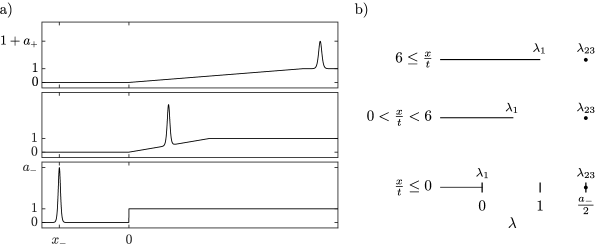
Figure 14: a) Soliton transmission through a RW when $a_{-}>2c^{2}$. b) The variation of the associated soliton-RW spectrum $\mathcal{S}_{1}^{(23)}$. Here, $c=1$ without loss of generality.

There are a number of implications of eq. (3.35), which we now investigate. First, we need to distinguish between where the soliton center $x_{0}$ is initialized. When $x_{0}>0$, the soliton always outruns the mean field because the soliton characteristic (3.27) lies to the right of the RW fan (3.10) due to the velocity ordering (3.8). Thus, the case $x_{0}>0$ does not give rise to soliton-RW interaction.

When $x_{0}<0$, there are two possibilities—soliton transmission or soliton trapping—the determination of which is based on the spatio-temporal structure of the spectrum $\mathcal{S}_{1}$. Soliton transmission requires that the spectrum remain of the collapsed type, i.e., of the form $\mathcal{S}_{1}^{(23)}$ (3.28). Soliton trapping occurs when the spectrum becomes the merged type $\mathcal{S}_{1}^{(12)}$ (3.20). The distinction boils down to the ordering of the Riemann invariants.

To examine this in detail, it will be useful to identify the initial soliton amplitude and position as $a_{-}=a_{0}$ and $x_{-}=x_{0}$, respectively, on the mean background $\overline{u}_{-}=0$, denoting the fact that the initial soliton is located on the negative $x$-axis.

When the initial soliton amplitude is sufficiently large ($a_{-}>2c^{2}$), we see in the example of Fig. 14 (where we set $c=1$ without loss of generality) that the spectrum $\mathcal{S}_{1}^{(23)}$ consists of the semi-infinite band describing the mean field and an eigenvalue corresponding to the soliton. The eigenvalue never intersects the semi-infinite band corresponding to soliton transmission because the eigenvalue persists. Contrast that with the example in Fig. 15 (again with $c=1$) where the semi-infinite band overtakes the spectral point for $x>6c^{2}t$. This case corresponds to a sufficiently small initial soliton amplitude $0<a_{-}\leq 2c^{2}$ and is associated with soliton trapping.

Now we describe the details of soliton-RW transmission. Since $\lambda_{23}(x,t)=a_{-}/2>c^{2}$, we can identify the transmitted soliton by its amplitude $a_{+}$ propagating on the mean $u_{+}=c^{2}$. By the constancy of $\lambda_{23}$ and the mapping in eq. (3.25), we have the relationship

$$\frac{a_{-}}{2}+\overline{u}_{-}=\frac{a_{+}}{2}+\overline{u}_{+}.$$ (3.36)

The transmitted soliton amplitude $a_{+}$ is determined solely in terms of the jump in the mean $c^{2}$ and the incident soliton amplitude $a_{-}$. More generally, the soliton amplitude field $a(x,t)$ is determined by the constancy of $\lambda_{23}$ according to

$$\begin{split}a(x,t)&=a_{-}-2\overline{u}(x,t)=\begin{cases}a_{-}&x\leq 0,\\[8.53581pt] \displaystyle a_{-}-\frac{x}{3t}&0<x<6c^{2}t,\\[8.53581pt] a_{+}&6c^{2}t<x\end{cases}.\end{split}$$ (3.37)

Knowing $\lambda_{1}(x,t)$ and $\lambda_{23}$ or, equivalently, the amplitude field and the mean field, we can determine the soliton trajectory $x_{s}(t;x_{-})$ by integrating the characteristic equation (3.27)

$$x_{s}(t;x_{-})=\begin{cases}x_{-}+2a_{-}t&t\leq t_{*}\\ 3a_{-}t^{1/3}\left(t^{2/3}-t_{*}^{2/3}\right)&t_{*}<t<t_{**}\\ x_{+}+(2a_{+}+6c^{2})t&t_{**}\leq t\end{cases},$$ (3.38)

where

$$t_{*}=\frac{|x_{-}|}{2a_{-}},\quad t_{**}=\left(\frac{a_{-}}{a_{+}}\right)^{3/2}t_{*},\quad x_{+}=\left(\frac{a_{-}}{a_{+}}\right)^{1/2}x_{-}.$$ (3.39)

The soliton amplitude as a function of time is therefore eq. (3.37) evaluated at $x=x_{s}(t;x_{-})$. The difference between the post and pre interaction $x$-intercepts of the soliton trajectory is its phase shift due to RW interaction

$$\Delta=x_{+}-x_{-}=\left(\sqrt{\frac{a_{-}}{a_{+}}}-1\right)x_{-}.$$ (3.40)

Since $a_{-}>a_{+}$ and $x_{-}<0$, the soliton phase shift is negative $\Delta<0$.

The results for the soliton trajectory (3.38) and phase shift (3.40), obtained by modulation theory, are the same as the results we obtained in Sec. (2.2.1) using soliton perturbation theory.

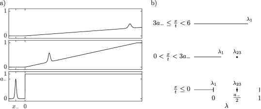
Figure 15: a) Soliton trapping by a RW when $0<a_{-}\leq 2c^{2}$. b) Variation of the associated soliton-RW spectrum $\mathcal{S}_{1}^{(23)}$. The soliton never overtakes the RW because for $x>3a_{-}t$, the semi-infinite spectral band absorbs the collapsed band. Here, $c=1$ without loss of generality.

There is an alternative way to determine the soliton phase shift due to RW interaction. For this, we utilize the additional Riemann invariant for the 1-phase Whitham modulation equations when $0<\lambda_{3}-\lambda_{2}\ll 1$, in which the cnoidal wave exhibits the small wavenumber (cf. eq. (3.12))

$$k\sim-\frac{2\pi\sqrt{\lambda_{3}-\lambda_{1}}}{\ln(\lambda_{3}-\lambda_{2})}\ll 1.$$ (3.41)

This small wavenumber regime corresponds to a weakly interacting soliton train [31, 2]. We now consider the interaction of this soliton train with a RW modeled by the 1-wave solution of the 1-phase Whitham modulation equations (3.13) in which $\lambda_{2}$, $\lambda_{3}$ are constant and $\lambda_{1}=\lambda_{1}(x/t)$ varies in a continuous, self-similar fashion, i.e., it is piecewise defined satisfying either $v_{1}(\boldsymbol{\lambda})=x/t$ or $\lambda_{1}$ constant. For $0<\lambda_{3}-\lambda_{2}\ll 1$, the 1-phase Whitham equations are close to the soliton limit and can be approximated as such, i.e., $v_{1}\sim 6\lambda_{1}$ (cf. (3.23)), $\lambda_{1}\sim\overline{u}$ is approximately the RW solution (3.31), and $\lambda_{3}\sim a_{-}/2$ as in (3.35). The additional modulation parameter $\lambda_{2}$ determines the small modulation wavenumber (3.41), which can be shown to approximately satisfy the conservation of waves in the form

$$k_{t}+\left(sk\right)_{x}=0,$$ (3.42)

where $s$ is the soliton velocity (3.26). To determine this 1-wave solution, we must select a value of $\lambda_{2}$. We now show that the specific value of $\lambda_{2}$, other than it being close to $\lambda_{3}$, is irrelevant for our purposes.

Considering the initial data (3.30) for $\lambda_{1}$, constant $\lambda_{2}$, $\lambda_{3}$ determines a relationship between the wavenumber (3.41) $k=k_{-}$ for $x<0$ and $k=k_{+}$ for $x>0$ where

$$k_{-}\sim-\frac{2\pi\sqrt{\lambda_{3}}}{\ln(\lambda_{3}-\lambda_{2})},\quad k_{+}\sim-\frac{2\pi\sqrt{\lambda_{3}-c^{2}}}{\ln(\lambda_{3}-\lambda_{2})}.$$ (3.43)

The ratio $k_{-}/k_{+}$ is independent of $\lambda_{2}$ so we can take the zero wavenumber, soliton limit to obtain

$$\lim_{\lambda_{2}\to\lambda_{3}}\frac{k_{-}}{k_{+}}=\sqrt{\frac{\lambda_{23}}{\lambda_{23}-c^{2}}}=\sqrt{\frac{a_{-}}{a_{+}}}.$$ (3.44)

The quantity $k_{-}/k_{+}$ is an invariant of the modulation dynamics in the soliton limit that determines the soliton phase shift $\Delta$ (3.40) due to RW interaction. Conservation of waves motivate the defining relationship

$$\lim_{\lambda_{2}\to\lambda_{3}}\frac{k_{-}}{k_{+}}=\frac{x_{+}}{x_{-}},$$ (3.45)

which verifies $\Delta$ in (3.40). The way to interpret this is through the concept of a weakly interacting soliton train. What we have shown in (3.44) is that for any $k_{-}>0$ sufficiently small, the 1-wave modulation solution satisfies

$$k_{+}\sim\sqrt{\frac{a_{+}}{a_{-}}}k_{-},\quad k_{-}\to 0.$$ (3.46)

Since $2\pi/k$ is the pulse spacing, we can track the propagation of two adjacent pulses of the weakly interacting soliton train, one located at $x=x_{-}<0$, and the other at $x_{-}-2\pi/k_{-}$. Each pulse’s propagation traces out a characteristic, which are well-separated by $2\pi/k_{-}$ for $x<0$. By the conservation of $\lambda_{2}$ and $\lambda_{3}$, the two characteristics will be well-separated by the distance $2\pi/k_{+}$ when $x>6c^{2}t$. Therefore, we can measure the phase shift of the pulse initially at $x=x_{-}$ by its position shift relative to the other pulse, i.e.

$$\Delta=x_{+}-x_{-}=\left(\frac{2\pi/k_{+}}{2\pi/k_{-}}-1\right)x_{-}\sim\left(\sqrt{\frac{a_{-}}{a_{+}}}-1\right)x_{-},$$ (3.47)

by using (3.46). Taking the soliton limit $k_{-}\to 0$, we obtain the same result (3.40) found by direct integration of the soliton characteristic. This physically inspired approach to determining the soliton phase shift will prove to be applicable to soliton-DSW interaction as well.

As noted earlier, when $0<a_{-}<2c^{2}$, the initial soliton becomes trapped in the interior of the RW. The soliton’s characteristic $x_{s}(t;x_{-})$ is the same as that given in eq. (3.38) except $t_{**}\to\infty$. The soliton amplitude in the interior of the RW is (3.37) evaluated at $x=x_{s}(t;x_{-})$ for $t>t_{*}$

$$a_{s}(t)=a_{-}\left(\frac{t_{*}}{t}\right)^{2/3}=a_{-}^{1/3}\left(\frac{|x_{-}|}{2t}\right)^{2/3},$$ (3.48)

hence decays algebraically as $t\to\infty$. To see that the soliton is trapped, we note that its velocity satisfies

$$\frac{\mathrm{d}x_{s}}{\mathrm{d}t}=a_{-}\left(3-\left(\frac{t_{*}}{t}\right)^{2/3}\right)\leq 3a_{-}<6c^{2},$$ (3.49)

therefore, its characteristic cannot overtake the right edge of the RW with velocity $6c^{2}$.

conditions	result	amplitude	position
$x_{0}>0$	no interaction
$x_{0}<0$, $a_{-}>2c^{2}$	transmission	$a_{+}=a_{-}-2c^{2}$	$\Delta/x_{0}=\sqrt{a_{-}/a_{+}}-1$
$x_{0}<0$, $a_{-}<2c^{2}$	trapping	$a_{s}(t)=a_{-}^{1/3}\left(\frac{|x_{0}|}{2t}\right)^{2/3}$	$x_{s}(t)=3a_{-}\left(t-\left(t\frac{x_{0}^{2}}{4a_{-}^{2}}\right)^{1/3}\right)$

Table 1: Predictions for soliton-RW interaction with a RW emanating from $x=0$ at $t=0$ and an initial soliton of amplitude $a_{-}$ centered at $x=x_{0}$ with $|x_{0}|\gg 1$. $a_{+}$ and $\Delta$ are the transmitted soliton amplitude and phase shift, respectively; $a_{s}(t)$ and $x_{s}(t)$ are the trapped soliton amplitude and position, respectively.

We summarize our findings for soliton-RW interaction in Table 1, all of which agree with the results obtained in Sec. 2 using soliton perturbation theory.

3.3 Soliton-Dispersive Mean Field Interaction: 2-phase modulations

Recall that a DSW resulting from the Riemann problem is described by a special solution (3.16) of the 1-phase Whitham equations. A soliton propagating on a slowly varying mean field is described by the degenerate 1-phase Whitham equations (3.24) in which the mean field evolves independent of the soliton. In order to describe the interaction of a soliton and a DSW, the modulations must simultaneously represent both the DSW and the soliton. As we now demonstrate, this is achieved by consideration of the degenerate 2-phase Whitham equations (3.5) with a collapsed spectral profile, either $\mathcal{S}_{2}^{(23)}$ or $\mathcal{S}_{2}^{(45)}$ depicted in Fig. 16. We relate the modulation of the spectrum $\mathcal{S}_{2}^{(45)}$ to the problem of soliton-DSW transmission and modulations of $\mathcal{S}_{2}^{(23)}$ to soliton-DSW trapping. We provide a direct proof that the DSW modulation evolves independent of the soliton in the case of soliton-DSW transmission and we determine the soliton’s characteristic velocity in both the transmission and trapping cases.

Figure 16: Degeneration pathways for 2-phase spectrum $\mathcal{S}_{2}$. For soliton-DSW interaction, the collapsing cases when $\lambda_{2}\to\lambda_{3}$ and $\lambda_{4}\to\lambda_{5}$ correspond to the trapped and transmission scenarios, respectively. When $\lambda_{2}\to\lambda_{1}$ or $\lambda_{4}\to\lambda_{3}$, one band merges with another. These cases correspond to transmission and trapped linear wavepacket-DSW interaction, respectively (see Sec. 3.4).

First, we introduce convenient notation. Recalling the characteristic velocities (3.6) for the $N=2$ case, the entries of the 2x2 matrices $\mathrm{Q}$ and $\mathrm{P}$ are terms of the form

$$I_{r}^{n}(\lambda_{k})=\int_{\lambda_{2r-1}}^{\lambda_{2r}}\frac{(\lambda_{k}-\mu)\mu^{n}\,\mathrm{d}\mu}{R(\mu)},\quad r\in\{1,2\},\quad n\in\{0,1,2\},$$ (3.50)

where $R(\mu)=\sqrt{(\mu-\lambda_{1})(\mu-\lambda_{2})(\mu-\lambda_{3})(\mu-\lambda_{4})(\mu-\lambda_{5})}$. The hyperelliptic integrals (3.50) will be simplified to elliptic integrals upon following the degeneration pathways noted in Fig. 16. For the various degenerate cases we consider, it is helpful to define quantities associated with the decoupled 1-phase DSW modulation by the parameters $\lambda_{i}\leq\lambda_{j}\leq\lambda_{k}$

$$\begin{split}R_{ijk}(\mu)&\equiv\sqrt{(\mu-\lambda_{i})(\mu-\lambda_{j})(\mu-\lambda_{k})},\\ \\ m_{ijk}&\equiv\frac{\lambda_{j}-\lambda_{i}}{\lambda_{k}-\lambda_{i}},\quad V_{ijk}\equiv 2(\lambda_{i}+\lambda_{j}+\lambda_{k}).\end{split}$$ (3.51)

3.3.1 Soliton-DSW Transmission

We consider the soliton-DSW interaction resulting from step down initial data (1.6) ($-$ sign) and approximate the initial soliton $v(x,0;x_{0})$ according to the spatially translated, modulated soliton

$$v(x,0;x_{0}=x_{-})=\lambda_{2}+2(\lambda_{45}-\lambda_{2})\mathrm{sech}^{2}\left(\sqrt{\lambda_{45}-\lambda_{2}}(x-x_{-})/\varepsilon\right),$$ (3.52a)

for $$x_{-}<0 \lambda_{45} \lambda_{2}$$ where is constant and is

$$\lambda_{2}(x,0)=\begin{cases}-1,&x<0,\\ 0,&x>0.\end{cases}$$ (3.52b)

The remaining spectral parameters are constant $\lambda_{1}=-1$, $\lambda_{3}=0$. We have scaled the step down to unit amplitude $c^{2}=1$ without loss of generality.

We remark that selecting piecewise constant initial data that leads to a global modulation solution for the Whitham equations is known as initial data regularization and was originally introduced in [67] (see also [91]).

For the case of soliton-DSW transmission, we consider the limit $\lambda_{4}\to\lambda_{5}$, resulting in the collapsed spectrum $\mathcal{S}_{2}^{(45)}$ depicted in Fig. 16. The asymptotics of the integrals (3.50) for $r=1$ when $\lambda_{4}\to\lambda_{5}$ are

$$I_{1}^{n}(\lambda_{k})\to\int_{\lambda_{1}}^{\lambda_{2}}\frac{(\lambda_{k}-\mu)\mu^{n}\,\mathrm{d}\mu}{(\lambda_{45}-\mu)R_{123}(\mu)},\quad\lambda_{4}\to\lambda_{5}.$$ (3.53)

These integrals can be expressed in terms of complete elliptic integrals. When $r=2$, the result depends upon $k$

$$I_{2}^{n}(\lambda_{k})\sim\begin{cases}\displaystyle\lambda_{5}^{n}\frac{(\lambda_{5}-\lambda_{k})\ln(\lambda_{5}-\lambda_{4})}{R_{123}(\lambda_{5})},&k\in\{1,2,3\},\\ \displaystyle\int_{\lambda_{3}}^{\lambda_{45}}\frac{\mu^{n}\,\mathrm{d}\mu}{R_{123}(\mu)},&k\in\{4,5\},\end{cases}\quad\lambda_{4}\to\lambda_{5}.$$ (3.54)

The integrals (3.54) for $k\in\{4,5\}$ can be expressed in terms of incomplete elliptic integrals.

We are now in a position to calculate the Whitham modulation velocities (3.6). When $k\in\{1,2,3\}$,

$$\begin{split}\lim_{\lambda_{4}\to\lambda_{5}}v_{k}&=-6(\lambda_{1}+\lambda_{2}+\lambda_{3}+2\lambda_{45})+12\lambda_{k}+\lim_{\lambda_{4}\to\lambda_{5}}12\frac{I_{2}^{2}(\lambda_{k})I_{1}^{0}(\lambda_{k})-I_{2}^{0}(\lambda_{k})I_{1}^{2}(\lambda_{k})}{I_{2}^{1}(\lambda_{k})I_{1}^{0}(\lambda_{k})-I_{2}^{0}(\lambda_{k})I_{1}^{1}(\lambda_{k})}\\ &=-6(\lambda_{1}+\lambda_{2}+\lambda_{3}+2\lambda_{45})+12\lambda_{k}+12\frac{\lambda_{45}^{2}I_{1}^{0}(\lambda_{k})-I_{1}^{2}(\lambda_{k})}{\lambda_{45}I_{1}^{0}(\lambda_{k})-I_{1}^{1}(\lambda_{k})}\\ &=-6(\lambda_{1}+\lambda_{2}+\lambda_{3}+2\lambda_{45})+12\lambda_{k}+12\frac{\displaystyle\int_{\lambda_{1}}^{\lambda_{2}}\frac{(\lambda_{45}+\mu)(\lambda_{k}-\mu)\,\mathrm{d}\mu}{R_{1}(\mu)}}{\displaystyle\int_{\lambda_{1}}^{\lambda_{2}}\frac{(\lambda_{k}-\mu)\,\mathrm{d}\mu}{R_{1}(\mu)}}\\ &=-6(\lambda_{1}+\lambda_{2}+\lambda_{3})+12\lambda_{k}+12\frac{\displaystyle\int_{\lambda_{1}}^{\lambda_{2}}\frac{(\lambda_{k}-\mu)\mu\,\mathrm{d}\mu}{R_{1}(\mu)}}{\displaystyle\int_{\lambda_{1}}^{\lambda_{2}}\frac{(\lambda_{k}-\mu)\,\mathrm{d}\mu}{R_{1}(\mu)}}.\end{split}$$ (3.55)

The last line is precisely the definition (3.6) of the 1-phase Whitham velocities (3.13) for the variables $\lambda_{1}$, $\lambda_{2}$, $\lambda_{3}$.

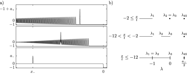
Figure 17: Soliton transmission through a DSW. a) Evolution of the solution $u(x,t)$. b) Evolution of the associated soliton-DSW spectrum $\mathcal{S}_{2}^{(45)}$.

For the cases $k\in\{4,5\}$, the integrals in (3.53) and (3.54) are independent of $\lambda_{4}$. Consequently, the velocities coalesce in the limit $v_{45}\equiv\lim_{\lambda_{4}\to\lambda_{5}}v_{4}=\lim_{\lambda_{4}\to\lambda_{5}}v_{5}$. After a calculation (the elliptic integral reference [68] is helpful), we obtain

$$\begin{split}v_{45}&=V_{123}+\frac{4(\lambda_{45}-\lambda_{2})}{1-\sqrt{\frac{(\lambda_{45}-\lambda_{2})(\lambda_{3}-\lambda_{1})}{(\lambda_{45}-\lambda_{3})(\lambda_{45}-\lambda_{1})}}Z(\varphi,m_{123})},\quad\sin{\varphi}=\sqrt{\frac{\lambda_{45}-\lambda_{3}}{\lambda_{45}-\lambda_{2}}}.\end{split}$$ (3.56)

The function

$$Z(\varphi,m)\equiv E(\varphi,m)-\frac{E(m)}{K(m)}F(\varphi,m)$$ (3.57)

is the Jacobian zeta function and involves the complete ($K(m)$, $E(m)$) and incomplete ($F(\varphi,m)$, $E(\varphi,m)$) elliptic integrals of the first and second kinds [68].

In the DSW’s harmonic limit $\lambda_{2}\to\lambda_{1}$, we have $m_{123}\to 0$ and $Z(\varphi,m_{123})\to 0$ so that the further degeneration (merger) of $\mathcal{S}_{2}^{(45)}$ results in the limiting characteristic velocity

$$\lim_{\lambda_{2}\to\lambda_{1}}v_{45}=2\lambda_{3}+4\lambda_{45},$$ (3.58)

which is the speed of a soliton associated with the eigenvalue $\lambda_{45}$ propagating on the mean $\lambda_{3}$ (cf. eq. (3.21)). In the DSW’s soliton limit $\lambda_{2}\to\lambda_{3}$, we have $\varphi=\pi/2+\mathcal{O}((\lambda_{3}-\lambda_{2})^{1/2})$ and $m_{123}=1+\mathcal{O}(\lambda_{3}-\lambda_{2})$ so that $Z(\varphi,m_{123})\to 0$ and the spectrum $\mathcal{S}_{2}^{(45)}$ further collapses. The resulting modulation velocity under this limit becomes

$$\lim_{\lambda_{2}\to\lambda_{3}}v_{45}=2\lambda_{1}+4\lambda_{45},$$ (3.59)

which is the speed of a soliton associated with $\lambda_{45}$ propagating on the mean $\lambda_{1}$.

Figure 17(a) details the case of a soliton with amplitude $a_{-}>0$ that is initially located at $x=x_{-}=x_{0}<0$ on the mean value $\overline{u}_{-}=0$. The negative step leads to the generation of a DSW with which the soliton interacts for some finite time. Post interaction, the soliton with amplitude $a_{+}>a_{-}$ on the background $\overline{u}_{+}=-c^{2}=-1$ (recall that we have scaled $c^{2}=1$) emerges to the right of the DSW. Its trajectory is $x_{s}(t)=(6\overline{u}_{+}+2a_{+})t+x_{+}$ and its phase shift due to DSW interaction is $\Delta=x_{+}-x_{-}$. We now interpret and analyze Fig. 17a) in terms of modulation theory.

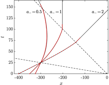
Figure 18: Soliton trajectories for the case of soliton-DSW transmission with varying incident soliton amplitudes $a_{-}\in\{0.5,1,2\}$. The solid curves are the characteristics (3.60) and the dots are the positions of the soliton extracted from numerical simulations of KdV (1.1) ($\varepsilon=1$) subject to (3.52). The dashed lines are the DSW’s space-time boundaries.

Figure 17(b) depicts the evolution of the spectrum $\mathcal{S}_{2}^{(45)}$ according to the GP DSW modulation solution (3.16). The modulation solution is a 2-wave in which only $\lambda_{2}$ varies with characteristic velocity $v_{2}$ while the other modulation variables are constant. The soliton’s trajectory $x_{s}(t)$ is completely determined by the characteristic

$$\frac{\mathrm{d}x_{s}}{\mathrm{d}t}=v_{45}(-1,\lambda_{2}(x_{s}/t),0,\lambda_{45},\lambda_{45}),\quad x_{s}(0)=x_{0}.$$ (3.60)

Since $v_{45}>v_{2}$ by strict hyperbolicity, the soliton trajectory $x_{s}(t)$ passes through the DSW if and only if the soliton is initialized to the left of the step: $x_{0}=x_{-}<0$. Prior to soliton-DSW interaction, the spectrum is doubly degenerate so that we identify (cf. eq. (3.25))

$$\lambda_{2}\to\lambda_{1}:\quad\lambda_{3}=\overline{u}_{-}=0,\quad\lambda_{45}=\frac{a_{-}}{2}+\overline{u}_{-}$$ (3.61a)

and the soliton velocity $$v_{45}$$ is (3.58). Post soliton-DSW interaction, the spectrum degenerates again so that we find the relations

$$\lambda_{2}\to\lambda_{3}:\quad\lambda_{1}=\overline{u}_{+}=-c^{2},\quad\lambda_{45}=\frac{a_{+}}{2}+\overline{u}_{+},$$ (3.61b)

and the soliton velocity $v_{45}$ is now (3.59). The four relations in (3.61) determine the constant modulation variables $\lambda_{1}$, $\lambda_{3}$, and $\lambda_{45}$ that, along with the GP modulation solution (3.16), are the soliton-DSW 2-wave modulation. But $\lambda_{45}$ is overdetermined, yielding a constraint on the soliton’s amplitude post DSW interaction

$$\frac{a_{+}}{2}+\overline{u}_{+}=\frac{a_{-}}{2}+\overline{u}_{-}.$$ (3.62)

This equation relating the soliton amplitude and mean field pre and post DSW interaction is the same as the relation (3.36) for soliton-RW interaction.

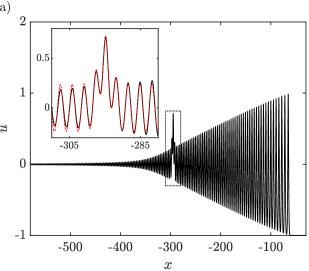
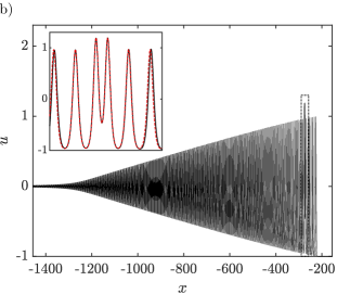
Figure 19: Numerical simulation of soliton-DSW transmission for $a_{-}=0.5$, $x_{-}=-325$ ($\lambda_{45}=0.25$). Insets: Local description of the simulation (solid, black curve) by the 2-phase solution with spectrum $\mathcal{S}_{2}^{(45)}(t)=(-\infty,-1]\cup[\lambda_{2}(x_{s}(t)/t),0]\cup\{\lambda_{45}\}$ (dashed, red curve). a) Snapshot at $t=30$. b) Snapshot at $t=109.3$.

By again introducing a non-interacting soliton train in which $0<\lambda_{5}-\lambda_{4}\ll\lambda_{45}$, the same argument as described in Sec. 3.2.3 for soliton-RW interaction also holds for soliton-DSW interaction, resulting in the same soliton phase shift as in eq. (3.47)

$$\Delta=x_{+}-x_{-}=\left(\sqrt{\frac{a_{-}}{a_{+}}}-1\right)x_{-}.$$ (3.63)

This time, $a_{-}<a_{+}$ so that the soliton phase shift due to DSW interaction is positive, $\Delta>0$. We will demonstrate that this is the same phase shift as obtained through (4.46) in the small dispersion IST analysis. Consistency requires that the direct integration of the soliton-DSW characteristic (3.60) yields the same phase shift as in eq. (3.63). We have numerically verified this to be the case, to the precision of the numerical method, by numerical integration of the characteristic equation (3.60) for a range of initial soliton amplitudes $a_{-}$.

Formulas (3.62) and (3.63) relate the soliton post DSW interaction to the soliton pre DSW interaction. We now investigate the predictions from modulation theory for the soliton during DSW interaction.

The soliton trajectories (3.60) in soliton-DSW transmission for different choices of $a_{-}$ are shown in Fig. 18. The 2-phase characteristics obtained by integrating eq. (3.60) (solid curves) compared with the soliton trajectories extracted from numerical simulations of the KdV equation (dots) are visually indistinguishable. Modulation theory can also be used to reconstruct an approximation to the full solution by inserting the modulation solution into the degenerate 2-phase solution ((3.1b) with $N=2$ in the limit $\lambda_{4}\to\lambda_{5}$)

$$u(x,t)=\lambda_{1}+\lambda_{2}+\lambda_{3}-2\mu_{1}(x,t)-2(\mu_{2}(x,t)-\lambda_{45}).$$ (3.64)

The functions $\mu_{1}$, $\mu_{2}$ satisfy the coupled nonlinear system (3.2), which we solve numerically. In fact, explicit representations of this solution have been obtained [30, 69, 70, 71] and we identify them as KdV breather solutions because they exhibit two time scales: one associated with their propagation and the other associated with their internal oscillations. In [71], $N+1$-phase solutions (3.1a) are analyzed in the case that $N$ finite bands collapse. This scenario describes $N$ breathers propagating on a cnoidal wave background. We use elevation, bright breathers to investigate the local structure of the solution within the vicinity of the soliton trajectory at certain times. Figure 19 displays a numerical simulation of soliton-DSW interaction for the case $a_{-}=0.5$, $x_{-}=-325$, corresponding to the trajectory shown in Fig. 18. At two different times, we plot the numerical solution. We also evaluate the DSW modulation solution $\lambda_{2}(x/t)$ (3.16) at $x=x_{s}(t)$ to obtain the local spectral profile $\mathcal{S}_{2}^{(45)}=(-\infty,\lambda_{1}]\cup[\lambda_{2},\lambda_{3}]\cup\{\lambda_{45}\}$ at the soliton characteristic $x_{s}(t)$ at time $t$. The remaining parameters $\lambda_{1}=-1$ and $\lambda_{3}=0$ are obtained from the initial step down and $\lambda_{45}=0.25$ corresponds to the initial soliton. The initial phases $\mu_{j}(0,0)$, $j=1,2$ for the 2-phase solution are chosen so that the 2-phase solution best matches the numerical simulation. The insets in Fig. 19 display the 2-phase solution for the spectrum $\mathcal{S}_{2}^{(45)}$ (dashed) overlaid on top of the numerical simulation (solid), showing excellent agreement in the vicinity of the soliton trajectory. The deviation is due to the modulation of the 2-phase wave which we have not incorporated into our approximate solution. At the early time depicted in Fig. 19(a), the soliton is interacting with the DSW harmonic edge and is approximately a linear superposition of a soliton and a cosine traveling wave. At the later time in Fig. 19(b), the soliton interacts with the DSW’s soliton edge. Here, the solution is approximately a soliton interacting with a soliton train. We have demonstrated that the KdV soliton-DSW interaction is well-described by a modulated bright breather solution of the KdV equation.

3.3.2 Soliton-DSW Trapping

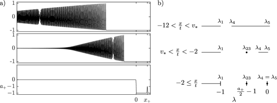
Figure 20: Soliton trapping by a DSW. a) Evolution of the solution $u(x,t)$. b) Evolution of the associated soliton-DSW spectrum $\mathcal{S}_{2}^{(23)}$.

We now consider the soliton-DSW interaction from step down initial data (1.6) ($-$ sign) and approximate the initial soliton $v(x,0;x_{0})$ according to the spatially translated, modulated soliton

$$v(x,0;x_{0}=x_{+})=\lambda_{4}+2(\lambda_{23}-\lambda_{4})\mathrm{sech}^{2}\left(\sqrt{\lambda_{23}-\lambda_{4}}(x-x_{+})/\varepsilon\right),$$ (3.65a)

where $$x_{+}>0 \lambda_{23} \lambda_{4}$$, is constant and there is an initial jump in

$$\lambda_{4}(x,0)=\begin{cases}-1&x<0,\\ 0&x>0,\end{cases}$$ (3.65b)

where we have scaled $c^{2}=1$, without loss of generality. The remaining spectral parameters are constant with the values $\lambda_{1}=-1$, $\lambda_{5}=0$ because the step has been scaled to unit amplitude. The reason for requiring the soliton to be located at $x=x_{+}>0$ is because the case where $x=x_{-}<0$ necessarily leads to soliton transmission as shown in the previous subsection.

An example numerical evolution of $u(x,t)$ and the modulation parameters is shown in Fig. 20. In contrast to the case of soliton-DSW transmission, the soliton eigenvalue $\lambda_{23}$ here eventually coincides with the DSW modulation solution $\lambda_{4}(x/t)$. This is the reason that the soliton is trapped.

For the soliton-DSW trapping problem, we require the asymptotics of the hyperelliptic integrals $I_{r}^{n}(\lambda_{k})$ (3.50) in the limit $\lambda_{2}\to\lambda_{3}$. For the characteristic velocity $v_{23}\equiv\lim_{\lambda_{2}\to\lambda_{3}}v_{2}=\lim_{\lambda_{2}\to\lambda_{3}}v_{3}$, note that

$$I_{1}^{n}(\lambda_{k})\sim\int_{\lambda_{1}}^{\lambda_{23}}\frac{\mu^{n}}{R_{145}(\mu)}\mathrm{d}\mu,\quad I_{2}^{n}(\lambda_{k})\sim\int_{\lambda_{23}}^{\lambda_{4}}\frac{\mu^{n}}{R_{145}(\mu)}\mathrm{d}\mu,\quad\lambda_{2}\to\lambda_{3}$$ (3.66)

when $k\in\{2,3\}$. These are incomplete elliptic integrals that, after inserting into equation (3.6) and simplifying, result in the soliton’s characteristic velocity

$$\begin{split}v_{23}&=V_{145}-4(\lambda_{5}-\lambda_{23})\frac{\sqrt{\frac{(\lambda_{4}-\lambda_{23})(\lambda_{23}-\lambda_{1})}{(\lambda_{5}-\lambda_{23})(\lambda_{5}-\lambda_{1})}}}{Z(\varphi,m_{145})},\quad\sin{\varphi}=\sqrt{\frac{\lambda_{23}-\lambda_{1}}{\lambda_{4}-\lambda_{1}}},\end{split}$$ (3.67)

where, again, $Z$ is the Jacobian zeta function (3.57).

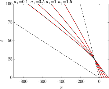
Figure 21: Soliton trajectories for the case of soliton-DSW trapping with varying incident soliton amplitudes $a_{+}\in\{0.1,0.5,1,1.5\}$. The solid curves are the characteristics (3.70) and the dots are the positions of the soliton extracted from numerical simulations of KdV (1.1) ($\varepsilon=1$) subject to (3.65). The dashed lines are the DSW’s space-time boundaries.

In the DSW’s soliton limit,

$$\lim_{\lambda_{4}\to\lambda_{5}}v_{23}=2\lambda_{1}+4\lambda_{23},$$ (3.68)

which is the speed of the soliton associated with $\lambda_{23}$ on the mean $\lambda_{1}$. When $\lambda_{4}\to\lambda_{23}$, we obtain

$$v_{*}\equiv\lim_{\lambda_{4}\to\lambda_{23}}v_{23}=2(\lambda_{1}+\lambda_{23}+\lambda_{5})-4(\lambda_{23}-\lambda_{1})\frac{(1-m_{*})K(m_{*})}{E(m_{*})-(1-m_{*})K(m_{*})},\quad m_{*}=\frac{\lambda_{23}-\lambda_{1}}{\lambda_{5}-\lambda_{1}}.$$ (3.69)

This is precisely the DSW modulation velocity $v_{4}(-1,\lambda_{23},0)=v_{*}$ (cf. $v_{2}$ in eq. (3.13)). Since $v_{4}(-1,\lambda_{4},0)<v_{*}$ for all $\lambda_{4}<\lambda_{23}$, the soliton cannot exit the DSW. It is trapped within the interior of the DSW and propagates no slower than $v_{*}$. In fact, this is not a true soliton solution; rather, it corresponds to the scenario of a pseudo soliton that is described in Sec. 4.

Figure 20(a) shows the evolution of a soliton with initial amplitude $0<a_{+}<2$ in front of the negative step $-c^{2}=-1$. The step generates a DSW that, upon interaction with the soliton, exhibits a defect. The defect manifests as a localized depression in the DSW’s envelope that resembles a dark envelope solitary wave. These are dark breather solutions of the KdV equation [30]. Although the dark breather migrates closer to the DSW harmonic, trailing edge, it remains trapped within the DSW.

Figure 20(b) depicts the evolution of the spectrum $\mathcal{S}_{2}^{(23)}$ according to the GP DSW modulation for $\lambda_{4}$ while the remaining $\lambda$s are constant. When $\lambda_{4}(x/t)<\lambda_{23}$, the modulation spectrum exhibits a merger into the 1-phase spectrum $(-\infty,-1]\cup[\lambda_{4}(x/t),0]$. This merger distinguishes soliton-DSW trapping from transmission.

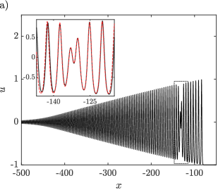
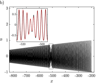
Figure 22: Numerical simulation of soliton-DSW trapping for $a_{+}=1$ ($\lambda_{23}=-0.5$) with 2-phase local description. Insets: Local description of the simulation (solid, black curve) by the 2-phase solution with spectrum $\mathcal{S}_{2}^{(23)}(t)=(-\infty,-1]\cup\{\lambda_{23}\}\cup[\lambda_{4}(x_{s}(t)/t),0]$ (dashed, red curve). a) Snapshot at $t=40$. b) Snapshot at $t=100$.

The soliton’s trajectory is completely determined by the characteristic

$$\frac{\mathrm{d}x_{s}}{\mathrm{d}t}=v_{23}(-1,\lambda_{23},\lambda_{23},\lambda_{4}(x_{s}/t),0),\quad x_{s}(0)=x_{+}.$$ (3.70)

So long as $\lambda_{23}<\lambda_{4}\leq 0$, $v_{23}<v_{4}$ so that a soliton initially located at $x=x_{+}>0$, will necessarily interact with the DSW forming behind it. Prior to soliton-DSW interaction, the spectrum is doubly degenerate so that we identify (cf. eq. (3.25))

$$\lambda_{4}\to\lambda_{5}:\quad\lambda_{1}=\overline{u}_{+}=-1,\quad\lambda_{23}=\frac{a_{+}}{2}+\overline{u}_{+}$$ (3.71)

then the soliton velocity $v_{23}$ is (3.68). The second eigenvalue $\lambda_{45}$ corresponds to the DSW’s soliton leading edge, which, from (3.16), is $\lambda_{45}=\overline{u}_{-}$. Therefore, the requirement on the initial soliton amplitude $a_{+}$ for soliton-DSW trapping is

$$\lambda_{23}<\lambda_{45}\quad\iff\quad a_{+}<2(\overline{u}_{-}-\overline{u}_{+}).$$ (3.72)

Trapped soliton trajectories, extracted from numerical simulations of KdV, are favorably compared in Fig. 21 with the characteristics (3.70). The local, 2-phase description of a trapped soliton is shown in Fig. 22. As in soliton-DSW transmission, the solution is locally described by a 2-phase solution whose spectrum ${\cal S}_{2}^{(23)}$ is determined by the DSW modulation evaluated on the soliton’s trajectory $\lambda_{4}(x_{s}(t)/t)$. Deviation between the 2-phase solution and the numerical simulation are due to the DSW modulation, which is not accounted for here.

During soliton-DSW interaction, the trapped soliton’s velocity $v_{23}$ decreases as $\lambda_{4}$ approaches $\lambda_{23}$. For $\lambda_{4}$ sufficiently close to $\lambda_{23}$, we can estimate the trapped soliton’s propagation. The modulation velocities admit the asymptotic expansions

$$\begin{split}v_{23}&\sim v_{*}+\frac{1}{3}G(\lambda_{1},\lambda_{23},\lambda_{5})(\lambda_{4}-\lambda_{23})+\cdots\\ v_{4}&\sim v_{*}+G(\lambda_{1},\lambda_{23},\lambda_{5})(\lambda_{4}-\lambda_{23})+\cdots,\end{split}$$ (3.73)

where

$$G(\lambda_{1},\lambda_{23},\lambda_{5})=2K(m_{*})\frac{(1-m_{*})(\lambda_{1}-3\lambda_{23}+2\lambda_{5})K(m_{*})-2(\lambda_{1}-2\lambda_{23}+\lambda_{5})E(m_{*})}{(\lambda_{5}-\lambda_{1})((1-m_{*})K(m_{*})-E(m_{*}))^{2}}.$$ (3.74)

Combining these asymptotic expansions with the modulation solution (3.16) evaluated at $x=x_{s}(t)$, we express the small parameter as

$$\lambda_{4}-\lambda_{23}\sim\frac{x_{s}(t)/t-v_{*}}{G}.$$ (3.75)

Then, expanding the characteristic ODE (3.70), we obtain

$$\frac{\mathrm{d}x_{s}}{\mathrm{d}t}\sim\frac{2}{3}v_{*}+\frac{x_{s}(t)}{3t},$$ (3.76)

which admits the general solution

$$x_{s}(t)\sim v_{*}t+Ct^{1/3},\quad C\in\mathbb{R}.$$ (3.77)

The trapped soliton’s velocity, as $\lambda_{4}$ approaches $\lambda_{23}$, asymptotes to the interior DSW modulation velocity $v_{*}$ as $t\to\infty$ with correction proportional to $t^{-2/3}$.

3.4 Linear Wavepacket-DSW interaction: 2-phase modulations

In the case of soliton-DSW interaction, we considered the collapsed spectra $\mathcal{S}_{2}^{(2\to 3)}$ and $\mathcal{S}_{2}^{(4\to 5)}$. It turns out that the consideration of the merged spectra $\mathcal{S}_{2}^{(1\to 2)}$ and $\mathcal{S}_{2}^{(3\to 4)}$, depicted in Fig. 16, can be used to describe the interaction of a linear wavepacket and a DSW. For completeness, we briefly report the degenerate 2-phase modulation velocities and refer the reader to [35] for more information on the application to wavepacket-DSW interaction.

First, we compute the limit $\lambda_{1}\to\lambda_{2}=\lambda_{12}$:

$$\begin{split}v_{12}&\equiv\lim_{\lambda_{1}\to\lambda_{2}}v_{1}=\lim_{\lambda_{1}\to\lambda_{2}}v_{2}\\ &=V_{345}-4K(m_{345})\frac{3\lambda_{12}^{2}-\lambda_{12}V_{345}+\lambda_{3}\lambda_{4}+\lambda_{3}\lambda_{5}+\lambda_{4}\lambda_{5}}{(\lambda_{5}-\lambda_{12})K(m_{345})-(\lambda_{5}-\lambda_{3})E(m_{345})}.\end{split}$$ (3.78)

The DSW modulation corresponds to the variation of $\lambda_{3}$, $\lambda_{4}$, and $\lambda_{5}$. In the DSW harmonic and soliton limits, we find $\lim_{\lambda_{4}\to\lambda_{3}}v_{12}=12\lambda_{12}-6\lambda_{5}$ and $\lim_{\lambda_{4}\to\lambda_{5}}v_{12}=12\lambda_{12}-6\lambda_{3}$, respectively, which corresponds to the linear group velocity $\omega_{k}=6\overline{u}-3\varepsilon^{2}k^{2}$ where $(k,\overline{u})=(2\sqrt{\lambda_{5}-\lambda_{12}},\lambda_{5})$ and $(k,\overline{u})=(2\sqrt{\lambda_{3}-\lambda_{12}},\lambda_{3})$, respectively. Because both of these limits exist, it corresponds to the case of linear wavepacket-DSW transmission.

Next, we compute the limit $\lambda_{3}\to\lambda_{4}=\lambda_{34}$:

$$\begin{split}v_{34}&\equiv\lim_{\lambda_{3}\to\lambda_{4}}v_{3}=\lim_{\lambda_{3}\to\lambda_{4}}v_{4}\\ &=V_{125}-4K(m_{125})\frac{3\lambda_{34}^{2}-\lambda_{34}V_{125}+\lambda_{1}\lambda_{2}+\lambda_{1}\lambda_{5}+\lambda_{2}\lambda_{5}}{(\lambda_{5}-\lambda_{34})K(m_{125})-(\lambda_{5}-\lambda_{1})E(m_{125})}.\end{split}$$ (3.79)

In this case, only the DSW harmonic limit corresponds to the linear group velocity $\lim_{\lambda_{2}\to\lambda_{1}}v_{34}=12\lambda_{34}-6\lambda_{5}$ where $(k,\overline{u})=(2\sqrt{\lambda_{5}-\lambda_{34}},\lambda_{5})$. The DSW soliton limit $\lambda_{2}\to\lambda_{5}$ cannot be reached. Instead, $\lim_{\lambda_{2}\to\lambda_{34}}v_{34}$ is the 1-phase modulation velocity corresponding to $v_{2}$ in (3.13). This corresponds to linear wavepacket-DSW trapping.

3.5 Discussion

The fact that the soliton’s trapping or transmission, amplitude (3.62), and phase shift (3.63) post dispersive hydrodynamic interaction only depend upon the boundary conditions and not on the details of the intermediate hydrodynamic state itself is a reflection of the isospectrality of the KdV equation. It is a generalization of soliton-soliton interaction and has been shown to approximately hold for a large class of nonlinear dispersive wave equations [2]. This property, termed hydrodynamic reciprocity, does not rely on the particular details of 2-phase modulation theory we have used here. Rather, all that is needed is a degenerate 1-phase modulation theory, which yields the existence of two adiabatic invariants that provide the needed relations. But this theory only describes the soliton pre and post hydrodynamic interaction.

Two phase modulation theory provides a detailed description of the solution structure and soliton trajectory during DSW interaction. When one of the bands in the 2-phase spectrum degenerately collapses, the new spectrum consists of a 1-phase spectrum, whose modulation corresponds to the DSW, and a single point corresponding to the soliton. This degenerate 2-phase solution is a KdV breather. The modulation velocity corresponding to the degenerate point spectrum determines the trajectory of the breather as it moves through the DSW. The soliton’s initial position $x_{0}$ and the location of the degenerate point in the spectrum determine the type of soliton-DSW interaction (transmission or trapping) and polarity of the breather (elevation/bright or depression/dark). The local structure of the soliton-DSW interaction is well-approximated by a breather solution.

While we used the degenerate Whitham velocities (3.56) and (3.67) to determine the trajectories of a soliton interacting with a DSW that results from step initial data, they can also be used to describe soliton propagation in other modulated 1-phase fields. For example, a localized disturbance [72], a DSW interacting with a RW [72, 73], or a DSW resulting from a cubic wavebreaking profile [54]. These modulation velocities could also be used to describe the boundaries of modulated 2-phase DSW-DSW interactions [55, 73].

4 Inverse Scattering Transform

In this section, the IST is applied to (1.1), which is an integrable equation. Unlike the other methods considered in this work, this approach is exact. The overview of the method is to construct eigenfunctions and scattering data for the time-independent Schrödinger scattering problem, i.e., the first half of the Lax pair (4.1). The potential of the Schrödinger operator is reconstructed through solving an associated integral equation. The time dependence of the scattering data is derived from the second half of the Lax pair (4.2), which yields the time evolution of the potential, i.e., the solution of the KdV equation. In this work, the potentials are not reflectionless, yet we still find discrete eigenvalues. Taking the far-field limit, when the soliton is well to the left or right of either a RW or DSW, we obtain exponentially accurate formulas that are found to agree with those obtained in the previous two sections by asymptotic expansions.

The IST for the KdV equation with rapidly decaying data relies on developing the inverse scattering associated with the time-independent Schrödinger equation (4.1), cf. [41, 42, 43, 44]. For step-like potentials without solitons, the inverse scattering for the time-independent Schrödinger equation was first analyzed in [45]. Over the years, the inverse scattering has been rigorously investigated and used to analyze the KdV equation for step-like initial data, cf. [46, 47, 48, 49].

4.1 General Scattering Theory Formulation

The linear Lax pair associated with (1.1) is

$$v_{xx}+\left(\frac{u(x,t)}{\varepsilon^{2}}+\frac{k^{2}}{\varepsilon^{2}}\right)v=0\leavevmode\nobreak\ ,$$ (4.1)

$$v_{t}=\left(u_{x}+\gamma\right)v+\left(4k^{2}-2u\right)v_{x}\leavevmode\nobreak\ ,$$ (4.2)

where $k$ is a time-independent spectral parameter and $\gamma$ a constant. In order to satisfy the compatibility condition $(v_{xx})_{t}=(v_{t})_{xx}$, the potential $u(x,t)$ must solve (1.1). Hence, the goal of this section is to find eigenvalues and eigenfunctions associated with the Schrödinger operator corresponding to step up/down BCs and from them reconstruct the potential. The eigenfunctions of (4.1) are characterized by their asymptotic behavior, cf. [51],

$$\phi(x,k)\sim e^{-\frac{ikx}{\varepsilon}},\ \ \ \overline{\phi}(x,k)\sim e^{\frac{ikx}{\varepsilon}}\leavevmode\nobreak\ ,\leavevmode\nobreak\ \leavevmode\nobreak\ \leavevmode\nobreak\ \leavevmode\nobreak\ \text{as}\leavevmode\nobreak\ x\rightarrow-\infty\leavevmode\nobreak\ ,$$ (4.3)

$$\psi(x,\lambda)\sim e^{\frac{i\lambda x}{\varepsilon}},\ \ \ \overline{\psi}(x,\lambda)\sim e^{-\frac{i\lambda x}{\varepsilon}}\leavevmode\nobreak\ ,\leavevmode\nobreak\ \leavevmode\nobreak\ \leavevmode\nobreak\ \leavevmode\nobreak\ \text{as}\leavevmode\nobreak\ x\rightarrow\infty\leavevmode\nobreak\ ,$$ (4.4)

where $\lambda(k)\equiv\sqrt{k^{2}\pm c^{2}}$, depending on the boundary condition as $x\rightarrow\infty$. Specifically, for the step up BCs ($+c^{2}$), $\lambda=\sqrt{k^{2}+c^{2}}$ and we take the branch cut $k\in[-ic,ic]$ so that $\text{sgn}(\Im k)=\text{sgn}(\Im\lambda)$. The values of $\lambda$ along the branch cut are located in the interval $[-c,c]$. If, on the other hand, we take step down BCs ($-c^{2}$), then $\lambda=\sqrt{k^{2}-c^{2}}$. In this case, we take the branch cut of $\lambda(k)$ to be $k\in[-c,c]$, which in the $\lambda$-plane corresponds to the imaginary interval $[-ic,ic]$ and again $\text{sgn}(\Im k)=\text{sgn}(\Im\lambda).$

The left (linearly independent) eigenfunctions can be expressed as a linear combination of the right eigenfunctions in the form

$$\phi(x,k)=b(k)\psi(x,\lambda(k))+a(k)\overline{\psi}(x,\lambda(k))\leavevmode\nobreak\ ,$$ (4.5)

$$\overline{\phi}(x,k)=\overline{a}(k)\psi(x,\lambda(k))+\overline{b}(k)\overline{\psi}(x,\lambda(k))\leavevmode\nobreak\ ,$$ (4.6)

where $k\in\mathbb{R}$. The coefficients are called the left scattering data and they are computed via

$$a(k)=\frac{\varepsilon}{2i\lambda}W(\phi,\psi)\leavevmode\nobreak\ ,\ \ b(k)=\frac{\varepsilon}{2i\lambda}W(\overline{\psi},\phi)\leavevmode\nobreak\ ,\ \ \overline{a}(k)=\frac{\varepsilon}{2i\lambda}W(\overline{\psi},\overline{\phi})\leavevmode\nobreak\ ,\ \ \overline{b}(k)=\frac{\varepsilon}{2i\lambda}W(\overline{\phi},\psi)\leavevmode\nobreak\ ,$$ (4.7)

where $W(f,g)\equiv fg_{x}-f_{x}g$. The scattering data can be expressed in terms of either $k$ or $\lambda$, which are related by $\lambda^{2}=k^{2}\pm c^{2},$ the $\pm$ sign depending on the BCs. On the other hand, the right eigenfunctions can be expressed in terms of the left eigenfunctions as

$$\psi(x,\lambda)=\alpha(k)\overline{\phi}(x,k(\lambda))+\beta(k)\phi(x,k(\lambda))\leavevmode\nobreak\ ,$$ (4.8)

$$\overline{\psi}(x,\lambda)=\overline{\alpha}(k)\phi(x,k(\lambda))+\overline{\beta}(k)\overline{\phi}(x,k(\lambda))\leavevmode\nobreak\ ,$$ (4.9)

where $\alpha(k)$, $\overline{\alpha}(k)$, $\beta(k)$ and $\overline{\beta}(k)$ are the right scattering data. When we analyze Eqn. (4.5)–(4.6) we say that we are solving the left scattering problem, and (4.8)–(4.9) is the right scattering problem. The left and right scattering data are related by

$$\overline{\alpha}(k)=\frac{\lambda}{k}\overline{a}(k)\leavevmode\nobreak\ ,\ \ \ \overline{\beta}(k)=-\frac{\lambda}{k}b(k)\leavevmode\nobreak\ ,\ \ \ \beta(k)=-\frac{\lambda}{k}\overline{b}(k)\leavevmode\nobreak\ ,\ \ \ \alpha(k)=\frac{\lambda}{k}a(k)\leavevmode\nobreak\ .$$ (4.10)

For values of $k,\lambda\in\mathbb{R}$, it can be shown that the eigenfunctions possess the following symmetries

$$\psi(x,-\lambda)=\overline{\psi}(x,\lambda)=\psi^{*}(x,\lambda)\leavevmode\nobreak\ ,\ \ \ \phi(x,-k)=\overline{\phi}(x,k)=\phi^{*}(x,k)\leavevmode\nobreak\ .$$ (4.11)

Below we derive a set of integral equations from the left (4.5) and right (4.8) scattering problems and with them compute solutions, where possible. A complete description of the soliton when it is inside either a RW or DSW is technical. Instead, we focus on soliton modes either well before or well after the interaction with either the RW or DSW. From this we are able to derive asymptotic soliton formulas with phase shift as well as give the transmission condition in terms of spectral parameters.

Both the step up and step down cases involve a similar calculation, hence we present them simultaneously with differences noted. The main difference between the two problems is the way in which the branch cut is taken for the different spectral parameter conditions. As a result, an additional term can appear in the integral equation that describes the system. We only consider phase shifts for the 1-soliton case because we are focused on the interaction of a single soliton with a RW or DSW mean field. Multi-soliton phase shifts can be calculated with a little more effort.

4.1.1 Right Scattering Problem

In this section, we consider the right scattering problem (4.8), where the right eigenfunctions are expressed as a linear combination of the left eigenfunctions. Doing so gives us insight into soliton modes that are initially placed well to left of the jump. To consider both boundary conditions simultaneously we use the notation $\pm$, where the top sign corresponds to the BC $u\rightarrow+c^{2}$ as $x\rightarrow\infty$ and the bottom sign to the BC $u\rightarrow-c^{2}$ as $x\rightarrow\infty$.

Define the right reflection coefficient $\widetilde{\rho}(k;t)\equiv-\frac{\overline{b}(k;t)}{a(k;t)}$ in terms of the scattering data given in (4.7). Then (4.8) is rewritten as

$$\frac{\psi(x,\lambda(k))}{a(k)}=\frac{\lambda}{k}\left[\leavevmode\nobreak\ \overline{\phi}(x,k)+\widetilde{\rho}(k)\phi(x,k)\right]\leavevmode\nobreak\ ,$$ (4.12)

where we have suppressed the time-dependence. We assume that $\phi$ and $\overline{\phi}$ have the following triangular forms

$$\phi(x,k)=e^{-\frac{ikx}{\varepsilon}}+\int_{-\infty}^{x}\widetilde{G}(x,s,t)e^{-\frac{iks}{\varepsilon}}ds\leavevmode\nobreak\ ,$$ (4.13)

$$\overline{\phi}(x,k)=e^{\frac{ikx}{\varepsilon}}+\int_{-\infty}^{x}\widetilde{G}(x,s,t)e^{\frac{iks}{\varepsilon}}ds\leavevmode\nobreak\ ,$$ (4.14)

with $\widetilde{G}(x,s,t)\equiv 0$ for $x>s$. From these integral forms one can show through a Green’s function that $\psi(x;k)$ and $\phi(x,k)$ are analytic in the upper half plane of both $k$ and $\lambda$. Consequently, the scattering data $a(k)$ defined in (4.7) is also analytic in the upper half plane. Next we substitute (4.13) and (4.14) into (4.12), and apply the Fourier transform $\frac{1}{2\pi\varepsilon}\int_{-\infty}^{\infty}e^{-\frac{i\lambda y}{\varepsilon}}d\lambda$ for $y<x$ and exploit the analyticity of $\phi(x,k),\psi(x,\lambda(k))$ and $a(k)$ in the upper half plane. The resulting Gel’fand-Levitan-Marchenko (GLM) equation obtained is

$$\widetilde{G}(x,y,t)+\widetilde{\Omega}(x+y,t)+\int_{-\infty}^{x}\widetilde{\Omega}(s+y,t)\widetilde{G}(x,s,t)ds=0\leavevmode\nobreak\ ,$$ (4.15)

where

$$\widetilde{\Omega}(z,t)=\frac{1}{2\pi\varepsilon}\int_{-\infty}^{\infty}\widetilde{\rho}(k;t)e^{-\frac{ikz}{\varepsilon}}dk-\widetilde{C}(t)e^{-\frac{\kappa_{0}z}{\varepsilon}}+\overline{\Omega}_{\pm}(z,t)\leavevmode\nobreak\ ,$$ (4.16)

with normalization constant

$$\widetilde{C}(t)=-\frac{i\overline{b}({k};t)}{\varepsilon\frac{\partial a}{\partial k}({k};t)}\bigg{|}_{k=ik_{0}}\leavevmode\nobreak\ ,\leavevmode\nobreak\ \leavevmode\nobreak\ \leavevmode\nobreak\ \leavevmode\nobreak\ \leavevmode\nobreak\ \leavevmode\nobreak\ k_{0}>0$$ (4.17)

and we remind the reader that $\pm$ represents the step up(+)/down(-) cases. The eigenvalue $k=ik_{0}$ is a simple zero of $a(k)$. A zero exists when $\kappa_{0}>c$ in the step up case and any $\kappa_{0}>0$ in the step down scenario. The eigenvalues satisfy $k_{0}\geq\kappa_{0}$ with equality at $\frac{\kappa_{0}x_{0}}{\varepsilon}=-\infty$. Note that $\overline{\Omega}_{-}(z,t)\equiv 0$ in (4.16) and

$$\overline{\Omega}_{+}(z,t)=\frac{1}{2\pi\varepsilon}\int_{0}^{c}\frac{\kappa e^{\frac{\kappa z}{\varepsilon}}}{\sqrt{c^{2}-\kappa^{2}}|a(i\kappa;t)|^{2}}d\kappa\leavevmode\nobreak\ .$$ (4.18)

This additional term is due to the branch cut $[-ic,ic]$ in the upper half $k$-plane for the step up boundary condition; the step down boundary condition has a branch cut lying on the real axis. The solution to the GLM equation in (4.15) is related to the potential by

$$u(x,t)=-2\varepsilon^{2}\frac{d}{dx}\widetilde{G}(x,x,t)\leavevmode\nobreak\ .$$ (4.19)

From the temporal equation of the Lax pair (4.2) we obtain the time-evolution of the scattering data where $\gamma=\frac{2i\lambda}{\varepsilon}(-2k^{2}\pm c^{2})$ and

$$a_{\pm}(k;t)=a_{\pm}(k;0)e^{i(4k^{3}-4k^{2}\lambda_{\pm}\pm 2c^{2}\lambda_{\pm})t/\varepsilon}\leavevmode\nobreak\ ,$$ (4.20)

$$\overline{b}_{\pm}(k;t)=\overline{b}_{\pm}(k;0)e^{-i(4k^{3}+4k^{2}\lambda_{\pm}\pm 2c^{2}\lambda_{\pm})t/\varepsilon}\leavevmode\nobreak\ ,$$

such that $\lambda_{\pm}(k)=\sqrt{k^{2}\pm c^{2}}$ corresponds to step up and step down, respectively. From this we obtain the time-evolution of the reflection coefficient

$$\widetilde{\rho}_{\pm}(k;t)=-\frac{\overline{b}_{\pm}(k;t)}{a_{\pm}(k;t)}=\widetilde{\rho}_{\pm}(k;0)e^{-8ik^{3}t/\varepsilon}\leavevmode\nobreak\ ,$$ (4.21)

and normalization constant

$$\widetilde{C}_{\pm}(t)=-\frac{i\overline{b}_{\pm}(k;t)}{\varepsilon\frac{\partial a_{\pm}(k;t)}{\partial k}}\bigg{|}_{k=ik_{0}}=\widetilde{C}_{\pm}(0)e^{-8k_{0}^{3}t/\varepsilon}\leavevmode\nobreak\ .$$ (4.22)

In order to obtain a solution to (4.15) we fix $t=0$ and then let $z\rightarrow-\infty$ so that the continuous spectrum in (4.16) goes to zero due to the Riemann-Lebesgue Lemma. Additionally, if we place a soliton initially far to the left of the origin ($x_{0}\ll-\varepsilon/\kappa_{0}$), then the branch cut term (4.18) also decays to zero exponentially fast leaving only the discrete spectrum term. Solving the resulting system for $\kappa_{0}>0$ we find

$$u(x,t)\sim 2\kappa_{0}^{2}\leavevmode\nobreak\ \text{sech}^{2}\left[\frac{\kappa_{0}}{\varepsilon}(x-4\kappa_{0}^{2}t-x_{0}^{\pm})\right]\leavevmode\nobreak\ ,\leavevmode\nobreak\ \leavevmode\nobreak\ \leavevmode\nobreak\ x_{0}^{\pm}=\frac{\varepsilon}{2\kappa_{0}}\log\left(-\frac{2\kappa_{0}}{\varepsilon\widetilde{C}_{\pm}(0)}\right)\leavevmode\nobreak\ .$$ (4.23)

This is the form of a soliton when it is far to the left of the initial jump ($k_{0}\approx\kappa_{0}$) and any subsequent radiation it emits.

4.1.2 Left Scattering Problem

Let us next consider the left scattering problem (4.5), where the left eigenfunctions are expressed as a linear combination of the right eigenfunctions. Here we will obtain a formula for the soliton when it is well to the right of the jump, where the radiation from the continuous spectrum is exponentially small. These formula describe a soliton which transmits left-to-right through either a RW or DSW. Again, when we write $\pm$, the top (bottom) sign corresponds to the step up (down) boundary condition at $x\rightarrow\infty$.

Begin by defining the reflection coefficient $\rho(\lambda;t)\equiv\frac{b(\lambda;t)}{a(\lambda;t)}$ in terms of the scattering data (4.7). Then (4.5) can be rewritten as

$$\frac{\phi(x,k(\lambda))}{a(\lambda)}=\rho(\lambda)\psi(x;\lambda)+\overline{\psi}(x;\lambda)\leavevmode\nobreak\ ,$$ (4.24)

where the time dependence has been suppressed. Next we assume that $\psi$ and $\overline{\psi}$ are expressed in the Volterra integral equations form

$$\psi(x,t;\lambda)=e^{\frac{i\lambda x}{\varepsilon}}+\int_{x}^{\infty}G(x,s,t)e^{\frac{i\lambda s}{\varepsilon}}ds\leavevmode\nobreak\ ,$$ (4.25)

$$\overline{\psi}(x,t;\lambda)=e^{-\frac{i\lambda x}{\varepsilon}}+\int_{x}^{\infty}G(x,s,t)e^{-\frac{i\lambda s}{\varepsilon}}ds\leavevmode\nobreak\ ,$$ (4.26)

with $G(x,s,t)\equiv 0$ when $s<x$. Again, $\phi(x,k(\lambda)),\psi(x,\lambda)$ and $a(\lambda)$ are analytic functions in the upper half plane of $\lambda$. Taking into account this analyticity we substitute (4.25) and (4.26) into (4.24) and then operate on the resulting equation by $\frac{1}{2\pi\varepsilon}\int_{-\infty}^{\infty}e^{\frac{i\lambda y}{\varepsilon}}d\lambda$ for $y>x$ to obtain the GLM integral equation

$$G(x,y,t)+\Omega(x+y,t)+\int_{x}^{\infty}\Omega(y+s,t)G(x,s,t)ds=0\leavevmode\nobreak\ ,\leavevmode\nobreak\ \leavevmode\nobreak\ y>x\leavevmode\nobreak\ ,$$ (4.27)

with kernel

$$\Omega(z,t)=\frac{1}{2\pi\varepsilon}\int_{-\infty}^{\infty}\rho(\lambda;t)e^{\frac{i\lambda z}{\varepsilon}}d\lambda-C(t)e^{-\frac{\eta_{0}z}{\varepsilon}}+\Omega^{\prime}_{\pm}(z,t)\leavevmode\nobreak\ ,$$ (4.28)

and normalization constant

$$C(t)=\frac{ib(\lambda;t)}{\varepsilon\frac{\partial a}{\partial\lambda}(\lambda;t)}\bigg{|}_{\lambda=i\ell_{0}}\leavevmode\nobreak\ ,$$ (4.29)

where $\lambda=i\ell_{0},\ell_{0}>0$ is a simple zero of $a(\lambda)$. In the step up case, $\Omega^{\prime}_{+}(z,t)\equiv 0$ and for step down there is an additional branch cut contribution of

$$\Omega^{\prime}_{-}(z,t)=\frac{1}{2\pi\varepsilon}\int_{0}^{c}\frac{\eta e^{-\frac{\eta z}{\varepsilon}}}{\sqrt{c^{2}-\eta^{2}}|\alpha(i\eta;t)|^{2}}d\eta\leavevmode\nobreak\ .$$ (4.30)

The potential can be related to the solution of the GLM equation in (4.27) by

$$u_{\pm}(x,t)=\pm c^{2}+2\varepsilon^{2}\frac{d}{dx}G(x,x,t)\leavevmode\nobreak\ ,$$ (4.31)

where the positive (negative) sign is taken in the $+c^{2}$ ($-c^{2}$) boundary condition case.

Next we find the time evolution of the relevant scattering data defined in (4.7) from (4.2). Here $\gamma=\frac{4ik^{3}}{\varepsilon}$ and so

$$a_{\pm}(\lambda;t)=a_{\pm}(\lambda;0)e^{i(4k_{\pm}^{3}-4k_{\pm}^{2}\lambda\pm 2c^{2}\lambda)t/\varepsilon}\leavevmode\nobreak\ ,$$ (4.32)

$$b_{\pm}(\lambda;t)=b_{\pm}(\lambda;0)e^{i(4k_{\pm}^{3}+4k_{\pm}^{2}\lambda\mp 2c^{2}\lambda)t/\varepsilon}\leavevmode\nobreak\ ,$$ (4.33)

where $k_{\pm}=\sqrt{\lambda^{2}\mp c^{2}}.$ The reflection coefficient and normalization constant that form the kernel in (4.28) are given, respectively, by

$$\rho_{\pm}(\lambda;t)=\frac{b_{\pm}(\lambda;t)}{a_{\pm}(\lambda;t)}=\rho_{\pm}(\lambda;0)e^{i(8k_{\pm}^{2}\lambda\mp 4c^{2}\lambda)t/\varepsilon}\leavevmode\nobreak\ ,$$ (4.34)

and

$$C_{\pm}(t)=C_{\pm}(0)e^{\ell_{0}(8k_{0}^{2}\pm 4c^{2})t/\varepsilon}\leavevmode\nobreak\ ,\leavevmode\nobreak\ \leavevmode\nobreak\ \leavevmode\nobreak\ C_{\pm}(0)=\frac{ib_{\pm}(\lambda;0)}{\varepsilon\frac{\partial a_{\pm}}{\partial\lambda}(\lambda;0)}\bigg{|}_{\lambda=i\ell_{0}}\leavevmode\nobreak\ ,$$ (4.35)

where $k_{0}^{\pm}=\sqrt{\ell_{0}^{2}\pm c^{2}}.$ CHECK THIS ONE Let us consider the case in which $\ell_{0}$ is significantly greater than $c$. Then as $t\rightarrow\infty$ the extra term in Eq. (4.30) decays in time and the only significant contribution to the kernel is the normalization constant term. From the reconstruction formula (4.31) we compute the 1-soliton solution in the $t\rightarrow\infty,x\gg 1$ asymptotic limit

$$u_{\pm}(x,t)\sim{\pm}c^{2}+2(\eta_{0}^{\pm})^{2}\leavevmode\nobreak\ \text{sech}^{2}\left[\frac{\eta_{0}^{\pm}}{\varepsilon}\left(x-(4(\eta_{0}^{\pm})^{2}{\pm}6c^{2})t-x_{s}^{\pm}\right)\right]\leavevmode\nobreak\ ,\leavevmode\nobreak\ \leavevmode\nobreak\ \leavevmode\nobreak\ x_{s}^{\pm}=\frac{\varepsilon}{2\eta_{0}^{\pm}}\log\left(-\frac{\varepsilon C_{\pm}(0)}{2\eta_{0}^{\pm}}\right)\leavevmode\nobreak\ ,$$ (4.36)

with $\eta_{0}^{\pm}=\sqrt{\kappa_{0}^{2}{\mp}c^{2}}>0$ corresponding to step up and step down, respectively. Here, we have taken the scale separation limit so that $\ell_{0}^{\pm}\rightarrow\eta_{0}^{\pm}$. At this point, the continuous spectrum contribution from the reflection coefficient in (4.28) is exponentially small. This is what we refer to as a proper soliton with a phase shift of $\Delta\equiv x_{s}^{\pm}-x_{0}.$

4.2 Discussion of IST Results

Let us discuss the significance of Eq. (4.36). Consider an initial soliton of the form (4.23) with $x_{0}\ll-\varepsilon/\kappa_{0}$ and step up BCs. Hence, the eigenvalue is $k_{0}$ ($\ell_{0}$) is exponentially close to $\kappa_{0}$ ($\eta_{0}$), the amplitude parameter. If $\kappa_{0}>c$, then the soliton will transmit through the resulting rarefaction wave and it will be of the form given by the positive root in (4.36). The transmitted soliton will be of smaller amplitude $(\eta_{0}^{+}<\kappa_{0})$, but larger velocity in comparison to the incident soliton. In terms of the scattering problem (4.1), this mode is a proper soliton and corresponds to a proper discrete eigenvalue [50]. The phase shift for this case is calculated below.

If on the other hand $\kappa_{0}<c$, then the soliton will become trapped within the rarefaction ramp, never reaching the top. In this case, formula (4.36) does not apply since there are no proper eigenvalues of the direct scattering problem; that is, eigenvalues with corresponding eigenfunctions that decay rapidly to zero as $|x|\rightarrow\infty$. Instead, the inverse scattering yields modes that resemble solitons until they reach the rarefaction ramp [50], hence we call them quasi or pseudo solitons. The terms of the inverse scattering that yield pseudo solitons were called pseudo-embedded eigenvalues, however they were not associated with zeros of scattering data like normal eigenvalues, rather they corresponded to the dominant contribution of the branch cut integral (4.18) for $-\infty<x_{0}\ll-\varepsilon/\kappa_{0}$. Indeed, a more recent work [27] has identified this case as corresponding to resonant poles that leave the imaginary axis. The associated eigenfunctions are not bound states. To be clear, proper solitons with true eigenvalues always transmit through a rarefaction wave. Finding explicit formula that describe the dynamics of the soliton while it is on the ramp from an IST point of view is an open problem.

We point out that if an initial soliton of the form in (4.36) with fixed $x_{0}^{+}=x_{0}>0$ and $\eta_{0}^{+}>0$ is taken, then the soliton will never become trapped since the right edge of the ramp moves to the right slower than the soliton.

Now let us examine (4.36) in the case of step down BCs. First, consider an initial soliton of the form (4.23) with $x_{0}\ll-\varepsilon/\kappa_{0}$. Again, we replace $\ell_{0}$ ($k_{0}$) with $\eta_{0}$ ($\kappa_{0}$) in the formulas. Regardless of the size of $\kappa_{0}$, this soliton will tunnel through the resulting DSW and when it reaches the other side, it will have a form like the negative root in (4.36). In this case $\eta_{0}^{-}=\sqrt{\kappa_{0}^{2}+c^{2}}>c$, so this is a proper soliton associated with a true eigenvalue and $L^{2}(\mathbb{R})$-eigenfunctions of (4.1). The transmitted soliton will have a larger amplitude $(\eta_{0}^{-}>\kappa_{0})$, but smaller velocity in comparison to the initial state. The phase shift is computed below.

The final case to consider is when a soliton is initially placed to the right of a step down. The initial condition will look like the negative root of (4.36) with fixed $x_{0}=x_{s}^{-}>0,\eta_{0}=\eta_{0}^{-}>0$ at $t=0$. The soliton can have positive, negative or zero velocity, depending on the amplitude relative to the step height. When $4\eta_{0}^{2}>6c^{2}$ ($4\eta_{0}^{2}<6c^{2}$) the soliton velocity is positive (negative); if $4\eta_{0}^{2}=6c^{2}$, the soliton velocity is zero. The DSW that emanates from the jump will have negative velocity. By the Whitham approach, the right (solitonic) edge of the DSW region moves with velocity $-2c^{2}$. A proper soliton corresponds to $\eta_{0}>c$ and has velocity greater than $-2c^{2}$; hence a proper soliton never reaches the right edge of the DSW. This is true even if the soliton has negative velocity since it is not negative enough to reach the nonlinear, soliton edge of the DSW. When $\eta_{0}<c$ the pseudo soliton velocity is less than $-2c^{2}$ and there is no true eigenvalue of (4.1) and thus no proper solitons. Here, the velocity of the pseudo soliton is less than $-2c^{2}$ and the pseudo soliton will eventually catch up to the DSW and embed itself inside it; i.e. the pseudo soliton will eventually become trapped. This is again an instance of a pseudo-embedded eigenvalue (resonant poles).

4.3 Spectral Data for a Soliton Mode plus Heaviside Initial Condition

Consider an initial condition of the form

$$u(x,t)=2\kappa_{0}^{2}\leavevmode\nobreak\ \text{sech}^{2}\left[\frac{\kappa_{0}}{\varepsilon}(x-x_{0})\right]\pm c^{2}H(x)\leavevmode\nobreak\ ,\leavevmode\nobreak\ \leavevmode\nobreak\ \leavevmode\nobreak\ x_{0}<0\leavevmode\nobreak\ ,$$ (4.37)

where $H(x)$ is the Heaviside function 1.4. The positive (negative) sign corresponds to step up (down) BCs and results in a RW (DSW). The associated half space initial eigenfunctions to (4.1) for the pure 1-soliton solution are

$$\phi(x,0)=e^{-\frac{ikx}{\varepsilon}}\left[1-\frac{2i\kappa_{0}}{(k+i\kappa_{0})\left(1+e^{-\frac{2\kappa_{0}(x-x_{0})}{\varepsilon}}\right)}\right]\leavevmode\nobreak\ ,\leavevmode\nobreak\ \leavevmode\nobreak\ \leavevmode\nobreak\ \leavevmode\nobreak\ x<0\leavevmode\nobreak\ ,$$ (4.38)

$$\psi(x,0)=e^{\frac{i\lambda x}{\varepsilon}}\left[1-\frac{2i\kappa_{0}}{(\lambda+i\kappa_{0})\left(1+e^{\frac{2\kappa_{0}(x-x_{0})}{\varepsilon}}\right)}\right]\leavevmode\nobreak\ ,\leavevmode\nobreak\ \leavevmode\nobreak\ \leavevmode\nobreak\ \leavevmode\nobreak\ x>0\leavevmode\nobreak\ .$$ (4.39)

The function in Eq. (4.38) can be obtained from the Rieman-Hilbert formulation of the inverse problem with one eigenvalue and zero reflection coefficient cf. [51]. The eigenfunctions $\overline{\phi}(x,0)$ and $\overline{\psi}(x,0)$ are obtained from the symmetry relations in (4.11). The scattering data is then computed from (4.7) and evaluated at $x=0$ to yield

$$a_{\pm}(\lambda;0)=\frac{(k_{\pm}+\lambda)\left[\kappa_{0}^{2}+k_{\pm}\lambda-i\kappa_{0}(k_{\pm}-\lambda)\text{tanh}\left(\frac{\kappa_{0}x_{0}}{\varepsilon}\right)\right]}{2\lambda(k_{\pm}+i\kappa_{0})(\lambda+i\kappa_{0})}\leavevmode\nobreak\ ,$$ (4.40)

$$b_{\pm}(\lambda;0)=\frac{(k_{\pm}-\lambda)\left[\kappa_{0}^{2}-k_{\pm}\lambda-i\kappa_{0}(k_{\pm}+\lambda)\text{tanh}\left(\frac{\kappa_{0}x_{0}}{\varepsilon}\right)\right]}{2\lambda(k_{\pm}+i\kappa_{0})(\lambda-i\kappa_{0})}\leavevmode\nobreak\ ,$$

such that $k_{\pm}\equiv\sqrt{\lambda^{2}\mp c^{2}}$ for the step up and step down cases, respectively. As a result, the reflection coefficient is

$$\rho_{\pm}(\lambda;0)={\frac{b_{\pm}(\lambda;0)}{a_{\pm}(\lambda;0)}}=\frac{(k_{\pm}-\lambda)(\lambda+i\kappa_{0})\left[\kappa_{0}^{2}-k_{\pm}\lambda-i\kappa_{0}(k_{\pm}+\lambda)\leavevmode\nobreak\ \text{tanh}\left(\frac{\kappa_{0}x_{0}}{\varepsilon}\right)\right]}{(k_{\pm}+\lambda)(\lambda-i\kappa_{0})\left[\kappa_{0}^{2}+k_{\pm}\lambda-i\kappa_{0}(k_{\pm}-\lambda)\leavevmode\nobreak\ \text{tanh}\left(\frac{\kappa_{0}x_{0}}{\varepsilon}\right)\right]}\leavevmode\nobreak\ .$$ (4.41)

This reflection coefficient is interesting from an integrability point of view since it is not reflectionless and it is exact. Let us now consider a soliton initially well-separated from the step, that is $x_{0}\ll-\varepsilon/\kappa_{0}$. In this case, the discrete eigenvalues are exponentially close to $\lambda_{\pm}=i\eta_{0}^{\pm}=i\sqrt{\kappa_{0}^{2}\mp c^{2}}$, where $\kappa_{0}$ is the amplitude parameter in (4.37). The normalization constant for $\kappa_{0}>c$ in the RW case and $\kappa_{0}>0$ in the DSW case is given by

$$\varepsilon C_{\pm}(0)=\frac{ib_{\pm}(\lambda;0)}{\frac{\partial a_{\pm}}{\partial\lambda}(\lambda;0)}\bigg{|}_{\lambda=i\eta_{0}}=$$ (4.42)

$$\frac{2\kappa_{0}^{2}\eta_{0}^{\pm}(\kappa_{0}+\eta_{0}^{\pm})^{3}\left[1+\tanh\left(\frac{\kappa_{0}x_{0}}{\varepsilon}\right)\right]}{-8\kappa_{0}^{4}(\kappa_{0}+\eta_{0}^{\pm})-c^{4}(5\kappa_{0}+\eta_{0}^{\pm})\pm c^{2}\kappa_{0}^{2}(11\kappa_{0}+5\eta_{0}^{\pm})+c^{2}\left[c^{2}(\kappa_{0}+\eta_{0}^{\pm})\mp\kappa_{0}^{2}(3\kappa_{0}+5\eta_{0}^{\pm})\right]\tanh\left(\frac{\kappa_{0}x_{0}}{\varepsilon}\right)},$$

where $\eta_{0}^{\pm}=\sqrt{\kappa_{0}^{2}{\mp}c^{2}}$ for step up and step down, respectively. From this formula we are able to calculate the IST phase shift below in both the step up and step down BC cases.

4.3.1 Scale Separation Asymptotics

There is a direct relationship between the soliton phase in (4.36) and the asymptotic phases in (2.30) and (3.40). Namely, in the limit $\frac{\kappa_{0}x_{0}}{\varepsilon}\ll-1$ the IST phase shift approaches that of the asymptotics. To see this, we compute the IST phase $x_{s}^{+}$ using the formulae given in (4.37)-(4.42) for $x_{0}<0$ with step up BCs. Within the normalization constant given in Eq. (4.42) the only place for scale separation effects is in the $\tanh\left(\frac{\kappa_{0}x_{0}}{\varepsilon}\right)$ terms. Taking the limit $\frac{\kappa_{0}x_{0}}{\varepsilon}\rightarrow-\infty$ and expanding $\tanh\left(\frac{\kappa_{0}x_{0}}{\varepsilon}\right)\approx-1+2e^{\frac{2\kappa_{0}x_{0}}{\varepsilon}}$ yields, to leading order, a normalization constant of

$$C_{+}(0)\rightarrow-\frac{2\kappa_{0}^{2}e^{\frac{2\kappa_{0}x_{0}}{\varepsilon}}}{\varepsilon\eta_{0}^{+}}\leavevmode\nobreak\ ,$$ (4.43)

where $\eta_{0}^{+}=\sqrt{\kappa_{0}^{2}-c^{2}}$. Substituting this into the phase formula of Eq. (4.36) shows

$$x_{s}^{+}\rightarrow\frac{\varepsilon}{2\eta_{0}^{+}}\log\left(\frac{\kappa_{0}^{2}e^{\frac{2\kappa_{0}x_{0}}{\varepsilon}}}{(\eta_{0}^{+})^{2}}\right)=\frac{\varepsilon}{2\eta_{0}^{+}}\log\left(\frac{\kappa_{0}^{2}}{(\eta_{0}^{+})^{2}}\right)+\frac{\kappa_{0}x_{0}}{\eta_{0}^{+}}\approx\frac{\kappa_{0}x_{0}}{\eta_{0}^{+}}=\frac{x_{0}}{\sqrt{1-\left(\frac{c}{\kappa_{0}}\right)^{2}}},$$ (4.44)

when $\varepsilon$ approaches zero; which is exactly the result in (2.30) and (3.40). Hence, both the soliton perturbation theory and Whitham modulation theory, in the small dispersion limit, reproduce the exact limiting phase shift of $\Delta\approx x_{0}(\kappa_{0}/\eta_{0}^{+}-1).$

Now consider step down BCs with a soliton placed to the left ($x_{0}<0$) of the jump. To obtain an asymptotic approximation we again take a small $\varepsilon$ limit in the normalization constant (4.42), similar to what was done in the RW case. Doing so yields

$$C_{-}(0)\rightarrow-\frac{2\kappa_{0}^{2}e^{\frac{2\kappa_{0}x_{0}}{\varepsilon}}}{\varepsilon\eta_{0}^{-}}\leavevmode\nobreak\ ,$$ (4.45)

as $\varepsilon\rightarrow 0$ for $\eta_{0}^{-}=\sqrt{\kappa_{0}^{2}+c^{2}}$. Substituting this into the phase given in Eq. (4.36) yields

$$x_{s}^{-}\rightarrow\frac{\varepsilon}{2\eta_{0}^{-}}\log\left(\frac{\kappa_{0}^{2}e^{\frac{2\kappa_{0}x_{0}}{\varepsilon}}}{(\eta_{0}^{-})^{2}}\right)\approx\frac{\kappa_{0}x_{0}}{\eta_{0}^{-}}=\frac{x_{0}}{\sqrt{1+\left(\frac{c}{\kappa_{0}}\right)^{2}}}\leavevmode\nobreak\ .$$ (4.46)

The resulting phase shift for a soliton through a DSW in the small dispersion limit is $\Delta\approx x_{0}(\kappa_{0}/\eta_{0}^{-}-1).$ Notice that this is exactly the phase shift produced by the Whitham approach in (3.63). In comparison to the RW asymptotic phase shift in Eq. (4.44), the only difference is the sign under the square root.

Using the asymptotic phase shift in (4.46) for the transmitted soliton ($x_{0}<0$) along with the leading (rightmost) edge of the DSW region ($x=-2c^{2}t$) obtained from Whitham theory, one can predict the time and position that the soliton will exit the DSW region. Namely, the soliton peak intersects the leading (solitonic) edge of the DSW region when $z(T_{2})=-2c^{2}T_{2}=4(\eta_{0}^{-})^{2}t+x_{s}^{-}$, or at time and position

$$T_{2}=-\frac{x_{0}}{4\kappa_{0}^{2}\sqrt{1+\frac{c^{2}}{\kappa_{0}^{2}}}},\leavevmode\nobreak\ \leavevmode\nobreak\ \leavevmode\nobreak\ z(T_{2})=\frac{x_{0}c^{2}}{2\kappa_{0}^{2}\sqrt{1+\frac{c^{2}}{\kappa_{0}^{2}}}},$$ (4.47)

respectively. These formulas were found to agree well with numerics.

Furthermore, the amount of time a tunneling soliton spends in the DSW region is approximately

$$T_{2}-T_{1}=-x_{0}\left(\frac{1}{4\kappa_{0}\sqrt{\kappa_{0}^{2}+c^{2}}}-\frac{1}{4\kappa_{0}^{2}+12c^{2}}\right),$$ (4.48)

where the incident time is given in (2.36). Asymptotically, this quantity goes to infinity as $x_{0}\rightarrow-\infty$ or $\kappa_{0}\rightarrow 0$. On the other hand, the time interval goes to zero as $x_{0}\rightarrow 0^{-}$ or $c\rightarrow\infty$ or $c\rightarrow 0$ or $\kappa_{0}\rightarrow\infty$.

4.4 IST Results

In this section, the results obtained from the IST are highlighted. It should be emphasized that these results are exponentially accurate for solitons well-clear of the RW or DSW. Where relevant, comparison with the asymptotic results obtained in Secs. 2 and 3 are shown.

4.4.1 Soliton-RW Results

The phase shift, $\Delta=x_{s}^{+}-x_{0}$, of a soliton that has tunneled through a RW is analytically calculated in two ways. First, in Eq. (4.36) the IST phase shift is found through the normalization constant in (4.42). The other means of approximating the phase shift is through the asymptotics and given in Eqs. (2.30) and (3.40).

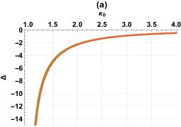
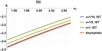
Figure 23: Phase shift of a soliton through a RW as a function of initial amplitude parameter $\kappa_{0}$. Other parameters: $x_{0}=-15,c=1$.

The IST phase shifts found through Eq. (4.36), for fixed $c$ and $x_{0}$, are plotted in Fig. 23 as a function of $\kappa_{0}$. The transmitted phase is less than the initial phase, indicating a negative phase shift. The magnitude of the shift is found to decrease as the incoming soliton amplitude relative to the step height increases. A larger amplitude means the step is small in comparison to the soliton and does not significantly affect it. In the limit $\kappa_{0}\rightarrow c^{+}$, the soliton phase shift approaches negative infinity which corresponds to trapping. The phase shift for different values of $\varepsilon$ are quite close, so it is difficult to distinguish between the cases. A close-up view of the curves in Fig. 23(b) shows clearly that as $\varepsilon$ decreases the IST result (exact) approaches the asymptotic result. This observation was already noted in Fig. 4 and was analytically established Sec. 4.3.1. Again, the asymptotic approaches considered are small dispersion limits of the exact IST results.

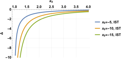
Figure 24: Phase shift of a soliton through a RW as a function of $\kappa_{0}$ for different values of the initial position $x_{0}$. Other parameters: $\varepsilon=1,c=1$.

Next, the phase shift for different initial positions is displayed in Fig. 24. The difference in the curves arises from the fact that the length of the ramp grows with time. Hence a soliton which starts further away from the ramp (more negative value of $x_{0}$) experiences a larger negative phase shift. Here we find the initial position and the magnitude of the phase shift are directly proportional to one another.

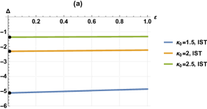
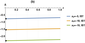
Figure 25: Phase shift of a soliton through RW as a function of dispersion parameter $\varepsilon$. Other parameters: (a) $x_{0}=-15,c=1$ and (b) $\kappa_{0}=2,c=1$. Black dots near $\varepsilon=0$ denote the corresponding asymptotic predictions found through Eqs. (2.30) and (3.40).

The next case to consider is when the dispersion parameter $\varepsilon$ is varied. The plots in Fig. 25 show that the phase shift does not vary much when $\varepsilon$ is relatively small ($0<\varepsilon\leq 1$). This is especially true when $\kappa_{0}$ is large, as Fig. 25(a) demonstrates. This suggests that for large $\kappa_{0}$ the asymptotic approximation will continue to provide reasonable approximation, even when $\varepsilon$ is not too small, i.e. provided the overall value of $\kappa_{0}/\varepsilon$ remains relatively large. The phase shift is found to be directly proportional to the (negative) parameter $x_{0}$ in Fig. 25(b); similar to what was observed in Fig. 24. Finally, both plots in Fig. 25 highlight that as $\varepsilon\rightarrow 0$ the IST formulae approach the asymptotic approximation.

Soliton Trapping

In this section, we consider the scenario of a soliton becoming trapped on a rarefaction ramp. In this case $\kappa_{0}<c$ (or $a_{-}<2c^{2}$) and there are no proper solitons in the IST. Instead there are so-called pseudo embedded eigenvalues (resonant poles) that yield pseudo solitons, which for $x_{0}\ll 1$ resemble solitons prior to soliton-RW interaction [50]. The evolution of a trapped soliton is displayed in Figs. 1(b) and 2(b). No matter how long the system is integrated forward in time, the solitary wave will not reach the top of the ramp. The absence of any true eigenvalues renders the soliton result in (4.36) inapplicable since it assumes that the soliton transmits through the RW.

4.4.2 Soliton-DSW Results

A step down boundary condition that generates a DSW is considered in this section. The primary case that our IST results can shed insight upon is when $x_{0}<0$ and the soliton is initially to the left of the jump. Here, the soliton always tunnels through the DSW. The phase shift of a transmitted soliton is calculated via asymptotic approximation and IST. When a soliton starts to the right of a step down ($x_{0}>0$), there are two outcomes: (a) soliton trapping (small amplitude) (b) no interaction with DSW (large amplitude). Again, the trapping case does not correspond to proper eigenvalues and is not discussed in detail here. A large amplitude initial condition does correspond to a genuine soliton (proper eigenvalue), but is not so interesting.

Soliton Initially Left of the Step, $x_{0}<0$

The typical evolution of a soliton initially placed to the left of the step down at the origin is shown in Fig. 3(a). Profiles corresponding to transmitted soliton results are presented in Fig. 26 for different values of $\varepsilon$. Three different approaches are compared: numerics, IST, and asymptotics. The IST approximation of the phase for a transmitted soliton is given in Eq. (4.36). The asymptotic approximation of the phase shifts are obtained through the Whitham (3.63) or the IST small dispersion limit (4.46). Indeed, Fig. 26 indicates overall good agreement between the different approaches, with the the asymptotic approximation improving as $\varepsilon\rightarrow 0$.

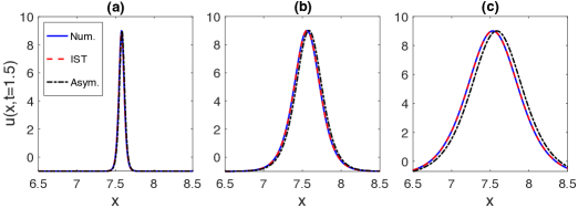
Figure 26: Soliton (post transmission) portion of the soliton-DSW solution for (a) $\varepsilon=1/10$, (b) $\varepsilon=1/2$, and (c) $\varepsilon=1$. Shown are numerical, IST, and asymptotic results. The initial condition used is (4.37) with parameters: $x_{0}=-15,\kappa_{0}=2,c=1$.

The phase shift for transmitted solitons is considered in more detail next. Recall the IST phase shift is defined by $\Delta=x_{s}^{-}-x_{0}$ for the soliton phase given in (4.36). The phase shift for different values of $\kappa_{0}$ is shown in Fig. 27. The figures indicate that the soliton always experiences a positive phase shift forward (opposite the RW case). Moreover, the phase shift approaches zero in the large amplitude limit, when $\kappa_{0}\rightarrow\infty$. What is also observed from Fig. 27(b) is that the phase shift curves approach the asymptotically derived formula derived in (4.46) and (3.63) as $\varepsilon\rightarrow 0$.

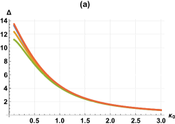
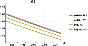
Figure 27: Phase shift of soliton through a DSW as a function of initial amplitude parameter $\kappa_{0}$ with varying $\varepsilon$. Other parameters: $x_{0}=-15,c=1$.

Next, consider when the initial position of the soliton is different, but still negative. The results in Fig. 28 show that the farther a soliton starts from the jump, the larger the phase shift it experiences. Intuitively, this makes since the length of the DSW region, $10c^{2}t$, grows with time, hence a soliton that encounters a DSW later in time experiences its dispersive effects for a longer duration. At fixed amplitude, the phase shift is inversely proportional to the initial position.

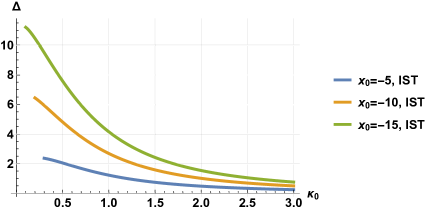
Figure 28: Phase shift of soliton through a DSW as a function of amplitude parameter $\kappa_{0}$ with varying $x_{0}$. Other parameters: $\varepsilon=1,c=1$.

The final set of phase shift figures to consider are those when $\varepsilon$ is varied. Two separate cases are considered in Fig. 29: different values of $\kappa_{0}$ [see Fig. 29(a)] and different values of $x_{0}$ [see Fig. 29(b)]. In both cases, the phase shift is positive and there is little variation in the curves for the range of $\varepsilon$ considered here, which are relatively small in magnitude. From Fig. 29(a) we note that the phase shift is inversely proportional to the amplitude. These figures show that the initial amplitude and position most significantly affect the soliton phase shift. As expected, the phase shift approaches the IST asymptotics and modulation theory prediction in Eqs. (4.46) and (3.63) as $\varepsilon\rightarrow 0$.

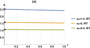
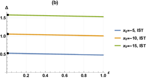
Figure 29: Phase shift of soliton through a DSW as a function of dispersion parameter $\varepsilon$. Other parameters: (a) $x_{0}=-15,c=1$ and (b) $\kappa_{0}=2,c=1$. Black dots near $\varepsilon=0$ denote the corresponding asymptotic predictions found through Eqs. (4.46) and (3.63).

We note recent, related work in which a mKdV soliton interacts propagates into an oscillatory wavetrain that asymptotes to a cnoidal wave solution as $x\to\infty$ [28]. The initial value problem is solved using Riemann-Hilbert methods. An amplitude threshold, similar to the requirement $\kappa_{0}>c$ for KdV soliton tunneling, is obtained in which the soliton completely penetrates the expanding, modulated cnoidal wavetrain.

Soliton Initially Right of the Step, $x_{0}>0$

A soliton that begins to the right of the ramp can either become trapped inside the DSW or not enter the DSW region at all. In the latter case, the solution resembles (2.39) and (4.36) for all $t>0$. Moreover, depending on the initial amplitude, the soliton will propagate with negative ($\eta_{0}<c\sqrt{3/2}$), positive ($\eta_{0}>c\sqrt{3/2}$), or zero ($\eta_{0}=c\sqrt{3/2}$) velocity. If $\eta_{0}<c\sqrt{3/2}$, but $\eta_{0}>c$, then the soliton moves with negative velocity, but never catches the solitonic edge of the DSW. For $\eta_{0}>c$, the soliton corresponds to a proper eigenvalue of the direct scattering problem and a proper soliton.

When $0<\eta_{0}<c$, there are no proper eigenvalues associated with the Schrödinger operator and this mode corresponds to a pseudo soliton [50]. The evolution of a soliton becoming trapped inside a DSW is shown in Fig. 3(b). The soliton reaches the solitonic edge of the DSW region at approximately the trapping time (2.40). Once inside the DSW region, the soliton takes a dark soliton breather form on the DSW background (see Fig. 20).

5 Conclusion

Separately, the evolution of solitons and jump-induced waves in the Korteweg-de Vries equation have been thoroughly studied. This work considered solutions composed of both a soliton and either a rarefaction wave or a dispersive shock wave, and their mutual interaction. Various analytical approaches, such as a soliton perturbation theory, Whitham modulation theory, and the Inverse Scattering Transform, are able to describe the evolution of these interactions and agree well with direct numerics. In particular, these methods are able to elucidate the phenomena of soliton tunneling and trapping and its dependence on the initial data of the soliton relative to the step. Furthermore, the step-up and step-down problems are found to be duals of each other and related via a principle known as reciprocity. From the point-of-view of the scattering data, this reciprocity condition is a relationship between the discrete eigenvalues and the jump height, corresponding to exact integrals of motion. Remarkably, the adiabatic invariants obtained via the asymptotic methods presented here predict precisely the same reciprocity condition.

The first method of analysis, soliton perturbation theory, benefits from being a general approach to soliton-mean interaction, so long as an approximate description of the mean field is available. This approach is particularly effective for soliton-RW interaction and can readily be extended to other evolutionary equations that admit solitary wave solutions. The second method of analysis, Whitham modulation theory, can similarly be extended to a broad class of evolutionary equations [2]. The primary limitation for both of these methods when applying them to non-integrable equations is obtaining a tractable, accurate, analytical description of soliton-DSW interaction. We overcome this limitation for the completely integrable KdV equation using multiphase Whitham modulation theory. The soliton-mean interaction is approximated with a 2-phase solution of the KdV equation whose associated Schrödinger operator’s $L^{\infty}(\mathbb{R})$ finite gap spectrum is allowed to vary slowly in space and time. Soliton-DSW interaction is a modulated bright or dark breather solution of the KdV equation, depending on whether the soliton is transmitted or trapped, respectively. The third method of analysis using the Inverse Scattering Transform results in the exact solution whose small dispersion limit is analyzed. In contrast to multiphase Whitham modulation theory, the Schrödinger operator’s $L^{2}(\mathbb{R})$ spectrum is independent of time. The existence of a discrete eigenvalue implies the transmission of a soliton through a RW or a DSW and exactly determines the transmitted soliton’s amplitude. The spectrum in the trapped case does not correspond to discrete eigenvalues of decaying eigenfunctions, hence we refer to them pseudo solitons. All three methods of analysis asymptotically agree in the limit of a soliton initialized sufficiently far away from the step or, equivalently, in the small dispersion regime.

References

- [1] M. J. Ablowitz and H. Segur, Solitons and the inverse scattering transform, SIAM, Philadelphia, (1981).
- [2] M. D. Maiden, D. V. Anderson, N. A. Franco, G. A. El, and M. A. Hoefer, Solitonic Dispersive Hydrodynamics: Theory and Observation, Phys. Rev. Lett., 120 144101 (2018).
- [3] G. El and M. Hoefer, Dispersive shock waves and modulation theory, Physica D, 333 11-65 (2016).
- [4] M. D. Maiden, N. K. Lowman, D. V. Anderson, M. E. Schubert, and M. A. Hoefer, Observation of dispersive shock waves, solitons, and their interactions in viscous fluid conduits, Phys. Rev. Lett., 116 174501 (2016).
- [5] S. Trillo, G. Deng, G. Biondini, M. Klein, G. F. Clauss, A. Chabchoub, and M. Onorato, Experimental Observation and Theoretical Description of Multisoliton Fission in Shallow Water, Phys. Rev. Lett. 117 144102 (2016).
- [6] A. Berchet, B. Simon, A. Beaudoin, P. Lubin, G. Rousseaux, and S. Huberson, Flow Fields and Particle Trajectories beneath a Tidal Bore: A Numerical Study, International Journal of Sediment Research 33 351 (2018).
- [7] R. Chassagne, A. G. Filippini, M. Ricchiuto, and P. Bonneton, Dispersive and Dispersive-like Bores in Channels with Sloping Banks, J. Fluid Mech. 870 595 (2019).
- [8] M. Brühl, P. J. Prins, S. Ujvary, I. Barranco, S. Wahls, and P. L.-F. Liu, Comparative Analysis of Bore Propagation over Long Distances Using Conventional Linear and KdV-Based Nonlinear Fourier Transform, Wave Motion 111 102905 (2022).
- [9] M. Carr, P. Sutherland, A. Haase, K. Evers, I. Fer, A. Jensen, H. Kalisch, J. Berntsen, E. Părău, Ø. Thiem, and P. A. Davies, Laboratory Experiments on Internal Solitary Waves in Ice-Covered Waters, Geophysical Research Letters bf 46 12230 (2019).
- [10] L. Li, R. Pawlowicz, and C. Wang, Seasonal Variability and Generation Mechanisms of Nonlinear Internal Waves in the Strait of Georgia, Journal of Geophysical Research: Oceans 123 5706 (2018).
- [11] J. C. Harris and L. Decker, Intermittent Large Amplitude Internal Waves Observed in Port Susan, Puget Sound, Estuarine, Coastal and Shelf Science 194 143 (2017).
- [12] C. R. Jackson, An Atlas of Internal Solitary-like Waves and Their Properties, http://www.internalwaveatlas.com/Atlas2_index.html, Global Ocean Associates, 2004.
- [13] B. Wetzel, D. Bongiovanni, M. Kues, Y. Hu, Z. Chen, S. Trillo, J. M. Dudley, S. Wabnitz, and R. Morandotti, Experimental Generation of Riemann Waves in Optics: A Route to Shock Wave Control, Physical Review Letters 117 (2016).
- [14] J. Nuño, C. Finot, G. Xu, G. Millot, M. Erkintalo, and J. Fatome, Vectorial Dispersive Shock Waves in Optical Fibers, Communications Physics 2 (2019).
- [15] T. Bienaimé, M. Isoard, Q. Fontaine, A. Bramati, A. M. Kamchatnov, Q. Glorieux, and N. Pavloff, Quantitative Analysis of Shock Wave Dynamics in a Fluid of Light, Phys. Rev. Lett. 126 183901 (2021).
- [16] A. Bendahmane, G. Xu, M. Conforti, A. Kudlinski, A. Mussot, and S. Trillo, The Piston Riemann Problem in a Photon Superfluid, Nat. Commun. 13 1 (2022).
- [17] M. E. Mossman, M. A. Hoefer, K. Julien, P. G. Kevrekidis, and P. Engels, Dissipative Shock Waves Generated by a Quantum-Mechanical Piston, Nature Communications 9 4665 (2018).
- [18] X. Buelna, D. Gonzalez, A. Freund, and J. Eloranta, Study of Shock Waves and Solitons in Bulk Superfluid He 4, Phys. Rev. B 99 144518 (2019).
- [19] A. Di Carli, G. Henderson, S. Flannigan, C. D. Colquhoun, M. Mitchell, G.-L. Oppo, A. J. Daley, S. Kuhr, and E. Haller, Collisionally Inhomogeneous Bose-Einstein Condensates with a Linear Interaction Gradient, Phys. Rev. Lett. 125 183602 (2020).
- [20] M. E. Mossman, E. S. Delikatny, M. M. Forbes, and P. Engels, Stability in Turbulence: The Interplay between Shocks and Vorticity in a Superfluid with Higher-Order Dispersion, Phys. Rev. A 102 053310 (2020).
- [21] P. Qiu and Y. Feng, Fast Particles Overtaking Shock Front in Two-Dimensional Yukawa Solids, Phys. Rev. E 106 015203 (2022).
- [22] C. G. Hooper, P. D. Ruiz, J. M. Huntley, and K. R. Khusnutdinova, Undular Bores Generated by Fracture, Phys. Rev. E 104 044207 (2021).
- [23] P. A. P. Janantha, P. Sprenger, M. A. Hoefer, and M. Wu, Observation of Self-Cavitating Envelope Dispersive Shock Waves in Yttrium Iron Garnet Thin Films, Physical Review Letters 119 024101 (2017).
- [24] S. Ryskamp, M. A. Hoefer, and G. Biondini, Oblique Interactions between Solitons and Mean Flows in the Kadomtsev–Petviashvili Equation, Nonlinearity 34 3583 (2021).
- [25] S. Gavrilyuk and K.-M. Shyue, Singular Solutions of the BBM Equation: Analytical and Numerical Study, Nonlinearity 35 388 (2021).
- [26] S. K. Ivanov and A. M. Kamchatnov, Motion of Dark Solitons in a Non-Uniform Flow of Bose-Einstein Condensate, arXiv preprint, 2208.12283 (2022).
- [27] A. Mucalica and D. E. Pelinovsky, Solitons on the Rarefactive Wave Background via the Darboux Transformation, arXiv preprint, 2207.01040 (2022).
- [28] M. Girotti, T. Grava, R. Jenkins, K. McLaughlin, and A. Minakov, Soliton v. the Gas: Fredholm Determinants, Analysis, and the Rapid Oscillations behind the Kinetic Equation, arXiv preprint, 2205.02601 (2022).
- [29] G. A. El, Soliton Gas in Integrable Dispersive Hydrodynamics, J. Stat. Mech. 2021 114001 (2021).
- [30] E. A. Kuznetsov and A. V. Mikhailov, Stability of Stationary Waves in Nonlinear Weakly Dispersive Media, Sov. Phys. JETP 40 855 (1975).
- [31] G. B. Whitham, Linear and nonlinear waves, Wiley, New York (1974).
- [32] P. Sprenger, M. A. Hoefer, and G. A. El, Hydrodynamic Optical Soliton Tunneling, Phys. Rev. E, 97 032218 (2018).
- [33] G. Biondini, S. Li, and D. Mantzavinos, Soliton Trapping, Transmission, and Wake in Modulationally Unstable Media, Phys. Rev. E 98 (2018).
- [34] G. Biondini and J. Lottes, Nonlinear Interactions between Solitons and Dispersive Shocks in Focusing Media, Phys. Rev. E 99 022215 (2019).
- [35] T. Congy, G. A. El, and M. A. Hoefer, Interaction of Linear Modulated Waves and Unsteady Dispersive Hydrodynamic States with Application to Shallow Water Waves, J. Fluid Mech. 875 1145 (2019).
- [36] A. M. Kamchatnov and D. V. Shaykin, Propagation of Wave Packets along Intensive Simple Waves, Phys. Fluids 33 052120 (2021).
- [37] K. van der Sande, G. A. El, and M. A. Hoefer, Dynamic Soliton–Mean Flow Interaction with Non-Convex Flux, J. Fluid Mech. 928 A21 (2021).
- [38] J. A. Whitehead and K. R. Helfrich, The Korteweg-de Vries Equation from Laboratory Conduit and Magma Migration Equations, Geophys. Res. Lett. 13 545 (1986).
- [39] I. Egorova, Z. Gladka, V. Kotlyarov, and G. Teschl, Long-Time Asymptotics for the Korteweg–de Vries Equation with Step-like Initial Data, Nonlinearity 26 1839 (2013).
- [40] J. A. Leach and D. J. Needham, The Large-Time Development of the Solution to an Initial-Value Problem for the Korteweg–de Vries Equation: I. Initial Data Has a Discontinuous Expansive Step, Nonlinearity 21 2391 (2008).
- [41] L. Faddeev, Properties of the S-matrix of the one-dimensional Schrödinger equation, Amer. Math. Soc. Trans. Series 2, 65 129-166 (1967).
- [42] P. Deift and E. Trubowitz, Inverse scattering on the line, Comm. Pure Appl. Math., 32 121-252 (1979).
- [43] C. S. Gardner, J. M. Greene, M. D. Kruskal, and R. M. Miura, Method for solving the Korteweg-de Vries equation, Phys. Rev. Lett., 19 1095-1097 (1967).
- [44] V. A. Marchenko, Sturm-Liouville operators and applications, American Mathematical Soc., 373 (2011).
- [45] V. S. Buslaev and V. N. Fomin, An inverse scattering problem for the one-dimensional Schrödinger equation on the entire axis (In Russian), Vesnik Leninggrad Univ. 17 56-64 (1962).
- [46] A. Cohen, Solutions of the Korteweg-de Vries equation with steplike initial profile, Commun. Partial Diff. Eq., 9 751-806 (1984).
- [47] A. Cohen, and T. Kaeppler, Scattering and inverse scattering for steplike potentials in the Schrödinger equation, Indiana Univ. Jl., 9 127-180, (1985).
- [48] T. Aktosun, On the Schrödinger equation with steplike potentials, J. Math. Phys., 40 5289–5305 (1999).
- [49] I. Egorova, Z. Gladka, T. Luc Lange, and G. Teschl, Inverse scattering theory for Schrödinger operators with steplike potentials, Zh. Mat. Fiz. Anal. Geom., 11 123–158 (2015).
- [50] M. J. Ablowitz, X.-D. Luo, and J. T. Cole, Solitons, the Korteweg-de Vries equation with step boundary values, and pseudo-embedded eigenvalues, J. Math. Phys. 59 091406 (2018).
- [51] M. J. Ablowitz and P.A. Clarkson, Solitons, Nonlinear Evolution Equations and Inverse Scattering, Cambridge University Press, Cambridge, (1991).
- [52] M. J. Ablowitz and D. E. Baldwin, Dispersive shock wave interactions and asymptotics, Phys. Rev. E, 87 022906 (2013).
- [53] H. Flaschka, M. G. Forest, and D. W. McLaughlin, Multiphase averaging and the inverse spectral solution of the Korteweg-de Vries equation, Comm. Pure Appl. Math., 33 739–784 (1980).
- [54] A. Gurevich and L. Pitaevskii, Nonstationary structure of a collisionless shock wave, J. Exp. Theor. Phys., 38 291-297 (1974).
- [55] T. Grava and F.-R. Tian, The generation, propagation, and extinction of multiphases in the KdV zero-dispersion limit, Comm. Pure Appl. Math., 55 1569–1639 (2002).
- [56] E. Date and S. Tanaka, Periodic multi-soliton solutions of Korteweg-de Vries equation and Toda lattice, Prog. Theor. Phys., 59 107–125 (1976).
- [57] S. P. Novikov, The periodic problem for the Korteweg-de Vries equation, Func. Anal. Appl., 8 236-246 (1974).
- [58] P. D. Lax, Periodic solutions of the KdV equation, Comm. Pure Appl. Math., 28 141-188 (1975).
- [59] A. R. Its and V. B. Matveev, Schrödinger operators with finite-gap spectrum and N-soliton solutions of the Korteweg-de Vries equation, Theor. Mat. Phys., 23 343-355 (1975).
- [60] B. A. Dubrovin, Periodic problems for the Korteweg-de Vries equation in the class of finite band potentials, Func. Anal. Appl., 9 215-223 (1975).
- [61] B. Dubrovin, Functionals of the Peierls-Fröhlich type and the variational principle for the Whitham equations, in: Solitons, geometry, and topology: on the crossroad, American Mathematical Society Translations, Series 2, 179, 35-44, Amer. Math. Soc., Providence, R.I., (1997).
- [62] P. D. Lax and C. D. Levermore, The small dispersion limit of the Korteweg-de Vries equation, Comm. Pure Appl. Math., 36 253–290, 571–593, 809–830 (1983).
- [63] S. Venakides, The generation of modulated wavetrains in the solution of the Korteweg-de Vries equation, Comm. Pure Appl. Math., 38 883–909 (1985).
- [64] P. Deift, S. Venakides, and X. Zhou, New results in small dispersion KdV by an extension of the steepest descent method for Riemann-Hilbert problems, Int. Math. Res. Not., 1997 285–299 (1997).
- [65] G. A. El, A. L. Krylov, and S. Venakides, Unified approach to KdV modulations, Comm. Pure Appl. Math., 54 1243–1270 (2001).
- [66] C. D. Levermore, The hyperbolic nature of the zero dispersion KdV limit, Commun. Part. Diff. Eq., 13 495–514 (1988).
- [67] A. M. Bloch and Y. Kodama, Dispersive regularization of the Whitham equation for the Toda lattice, SIAM J. Appl. Math., 52 909–928 (1992).
- [68] P.F. Byrd and M.D. Friedman, Handbook of elliptic integrals for engineers and scientists, Springer-Verlag, New York, (1971).
- [69] X.-R. Hu, S.-Y. Lou, and Y. Chen, Explicit solutions from eigenfunction symmetry of the Korteweg-de Vries equation, Phys. Rev. E, 85 056607 (2012).
- [70] S.-Y. Lou, Consistent Riccati expansion for integrable systems, Stud. Appl. Math., 134 372–402 (2015).
- [71] M. Bertola, R. Jenkins, and A. Tovbis, Partial Degeneration of Finite Gap Solutions to the Korteweg-de Vries Equation: Soliton Gas and Scattering on Elliptic Background, arXiv preprint, 2210.01350 (2022).
- [72] G. A. El and R. H. J. Grimshaw, Generation of undular bores in the shelves of slowly-varying solitary waves, Chaos, 12 1015–1026 (2002).
- [73] M. J. Ablowitz, D. E. Baldwin, and M. A. Hoefer, Soliton generation and multiple phases in dispersive shock and rarefaction wave interaction, Physical Review E, 80 016603 (2009).
- [74] G. A. El, The Thermodynamic Limit of the Whitham Equations, Physics Letters A, 311 374 (2003).
- [75] M. J. Ablowitz, J. T. Cole, and I. Rumanov, Whitham equations and phase shifts for the Korteweg–de Vries equation, Proc. Roy. Soc. A, 476 20200300 (2020).
- [76] G. B. Whitham, Non-linear dispersive waves, Proc. Roy. Soc. A, 283 238–261 (1965).
- [77] R. Grimshaw, Slowly Varying Solitary Waves. I. Korteweg-de Vries Equation, Proc. R. Soc. Lond. A 368 359 (1979).
- [78] L. D. Landau, E. M. Lifshitz, Quantum mechanics, Pergamon Press, Oxford, (1965).
- [79] C. Bai, Scanning tunneling microscopy and its applications, Springer, New York, (2000).
- [80] R. P. Feynman, Simulating physics with computers, Int. J. Theor. Phys., 21 467–488 (1982).
- [81] A. C. Newell, Nonlinear tunnelling, J. Math. Phys., 19 1126–1133 (1978).
- [82] E. M. Wright, D. R. Heatley, and G. I. Stegeman, Emission of spatial solitons from nonlinear waveguides, Phys. Rep., 194 309–323 (1990).
- [83] D. Anderson, M. Lisak, B. Malomed, and M. Quiroga-Teixeiro, Tunneling of an optical soliton through a fiber junction, JOSA B, 11 2380–2384 (1994).
- [84] M. I. Rodas-Verde, H. Michinel, and V. M. Pérez-Garcia, Controllable soliton emission from a Bose-Einstein condensate, Phys. Rev. Lett., 95 153903 (2005).
- [85] A. Barak, O. Peleg, C. Stucchio, A. Soffer, and M. Segev, Observation of soliton tunneling phenomena and soliton ejection, Phys. Rev. Lett. 100 153901 (2008).
- [86] M. Peccianti, A. Dyadyusha, M. Kaczmarek, and G. Assanto, Escaping solitons from a trapping potential, Phys. Rev. Lett., 101 153902 (2008).
- [87] G. Assanto, A. A. Minzoni, M. Peccianti, and N. F. Smyth, Optical solitary waves escaping a wide trapping potential in nematic liquid crystals: modulation theory, Phys. Rev. A, 79 033837 (2009).
- [88] A. H. Sheinfux, M. Rechtsman, B. Osting, J. Marzuola, and M. Segev, Soliton dynamics in a diffracting trapping potential, in: CLEO: QELS_Fundamental Science, Opt. Soc. of America, p. QM3E.7 (2013).
- [89] T. Marest, et al., Longitudinal soliton tunneling in optical fiber, Opt. Lett. 42 2350–2353 (2017).
- [90] G. Biondini, G. A. El, M. A. Hoefer, and P. D. Miller, Dispersive hydrodynamics: preface, Physica D, 333 1–5 (2016).
- [91] M. A. Hoefer, et al., Dispersive and classical shock waves in Bose-Einstein condensates and gas dynamics, Phys. Rev. A, 74 023623 (2006).
- [92] R. Meppelink, et al., Observation of shock waves in a large Bose-Einstein condensate, Phys. Rev. A, 80 043606 (2009).
- [93] W. Wan, S. Jia, and J. W. Fleischer, Dispersive superfluid-like shock waves in nonlinear optics, Nat. Phys., 3 46–51 (2007).
- [94] G. Xu, M. Conforti, A. Kudlinski, A. Mussot, and S. Trillo, Dispersive dam-break flow of a photon fluid, Phys. Rev. Lett., 118 254101 (2017).
- [95] B. Wetzel, et al., Experimental generation of Riemann waves in optics: a route to shock wave control, Phys. Rev. Lett., 117 073902 (2016).
- [96] M. A. Hoefer and M. J. Ablowitz, Interactions of dispersive shock waves, Physica D, 236 44–64 (2007).
- [97] M. A. Hoefer, P. Engels, and J. J. Chang, Matter-wave interference in Bose-Einstein condensates: a dispersive hydrodynamic perspective, Physica D, 238 1311–1320 (2009).
- [98] G. A. El, V. V. Khodorovskii, and A. M. Leszczyszyn, Refraction of dispersive shock waves, Physica D, 241 1567–1587 (2012).
- [99] G. El, M. Hoefer, and M. Shearer, Dispersive and diffusive-dispersive shock waves for nonconvex conservation laws, SIAM Rev., 59 3–61 (2017).
- [100] N. K. Lowman and M. A. Hoefer, Dispersive hydrodynamics in viscous fluid conduits, Phys. Rev E, 88 023016 (2013).
- [101] N. K. Lowman and M. A. Hoefer, Dispersive shock waves in viscously deformable media, J. Fluid Mech., 718 524–557 (2013).
- [102] Y. S. Kivshar and B. A. Malomed, Dynamics of solitons in nearly integrable systems, Rev. Mod. Phys., 61 763–915 (1989).
- [103] T. Grava, Whitham modulation equations and application to small dispersion asymptotics and long time asymptotics of nonlinear dispersive equations, in: Rogue and Shock Waves in Nonlinear Dispersive Media, Lecture Notes in Physics, eds. M. Onorato, S. Resitori, and F. Baronio, Springer, Cham, 926 309–336 (2016).
- [104] G. El, Resolution of a shock in hyperbolic systems modified by weak dispersion, Chaos, 15 037103 (2005).
- [105] T. Congy, G. A. El, G. Roberti, and A. Tovbis, Dispersive Hydrodynamics of Soliton Condensates for the Korteweg-de Vries Equation, arXiv preprint, 2208.04472 (2022).