Improving Low-Resource Question Answering using Active Learning in Multiple Stages

Abstract

Neural approaches have become very popular in the domain of Question Answering, however they require a large amount of annotated data. Furthermore, they often yield very good performance but only in the domain they were trained on. In this work we propose a novel approach that combines data augmentation via question-answer generation with Active Learning to improve performance in low resource settings, where the target domains are diverse in terms of difficulty and similarity to the source domain. We also investigate Active Learning for question answering in different stages, overall reducing the annotation effort of humans. For this purpose, we consider target domains in realistic settings, with an extremely low amount of annotated samples but with many unlabeled documents, which we assume can be obtained with little effort. Additionally, we assume sufficient amount of labeled data from the source domain is available. We perform extensive experiments to find the best setup for incorporating domain experts. Our findings show that our novel approach, where humans are incorporated as early as possible in the process, boosts performance in the low-resource, domain-specific setting, allowing for low-labeling-effort question answering systems in new, specialized domains. They further demonstrate how human annotation affects the performance of QA depending on the stage it is performed.

1 Introduction

Machine Reading Question Answering (MRQA) is a challenging and important problem. Facilitating targeted information extraction from documents, it allows users to get fast, easy access to a vast amount of documents available. MRQA models generally need plenty of annotations, therefore several methods have been devised for augmenting data by generating new annotated samples, with the ultimate goal of improving quality of predictions. Some of these approaches show a real benefit in the downstream MRQA task; however, there is no work focusing on employing Language Models (LM) fine-tuned for generating question-answer pairs in low-resource, domain-specific settings, which are often observed in practice. In these cases, most of the times only few annotated samples are available, due to the specialized domain being usually vastly different from the publicly available labeled data of the source domain. Moreover, labeling in general is an expensive procedure, as it requires a significant amount of time from domain experts. However, we consider collecting and annotating a small set of samples (e.g. 200), accurately selected to boost performance of the MRQA model, feasible and not too expensive. In this work we introduce a novel approach that follows this idea.

Although Shakeri et al. (2020) show that a question-answer generation approach trained on SQuAD (Rajpurkar et al., 2016) transfers fairly well to other (similar) domains, this does not hold in general with datasets from specialized domains, which are very relevant in practice. Additionally, so far it stays unclear how few samples from the target domain, selected based on various criteria, affect the performance of the MRQA model when they are used in the training of the sample generation model as well. In this work, we explore a novel approach that enables this, together with investigating how employing Active Learning (AL), either at the data generation model or at the MRQA model, affects the overall performance of the MRQA task. We consider only a small set of documents from the target domain annotated in terms of questions and answers, in addition to a potentially large set of samples from a different, generic source domain. We also assume to have access to a large amount of unlabeled data (documents) available from the target domain, which is common in real scenarios (e.g. publications from PubMed when considering the medical domain). We then employ a state-of-the-art model for generating question-answer pairs on these documents from the target domain, to enrich our training sets with synthetic data. We study the application of AL in order to label those samples which are most relevant for increasing performance, with the aim of reducing the amount of labeled samples needed. We consider these labeled samples in both the data generation stage as well as for the MRQA model itself. Our experimental results show great improvements for the MRQA task considering two domain-specific datasets, namely TechQA (Castelli et al., 2019) and BioASQ (Tsatsaronis et al., 2015), with few samples specifically annotated for the data generation model.

In this work, our main contributions are the following: 1) We introduce a novel approach that combines data augmentation for MRQA via question-answer generation with Active Learning; 2) we identify the most relevant samples for AL by adapting to our setting scoring functions recently used for unsupervised quality assessment of machine translation; 3) we introduce a new sample relevance score specific to MRQA by coupling the generated samples with the downstream task, so that the MRQA model influences the data augmentation process as well; and 4) we perform extensive experiments to demonstrate how to utilize AL in MRQA for improving performance in low-resource, domain-specific scenarios.

2 Related Work

2.1 Low-Resource MRQA

In the literature, there are several approaches for tackling the low-resource problem, including scenarios where few labeled data are available and others where no labels are available at all.

One approach is to use pre-trained Language Models (Alberti et al., 2019; Radford et al., 2019; Lewis et al., 2019) backed by transformers (Vaswani et al., 2017), which can be especially useful in cases where little or no labeled data exists and it is costly to generate more. In the best case, the LM can be used without further fine-tuning (when the target task and domain is similar to those used in the pre-training objective). Otherwise, if unlabeled data is available, it may be used for adaptation of the LM in a self-supervised fashion.

If the low-resource domain is accompanied by some annotated samples, weak supervision – where external sources of information are used – becomes relevant  (Hedderich et al., 2021; Wang et al., 2019). Moreover, data augmentation (Zhang et al., 2020; Van et al., 2021) and LM domain adaptation (Nishida et al., 2020; Zhang et al., 2020) have been shown to improve performance for MRQA.

A different approach is to use domain transfer, where a model is trained on a source domain and then adapted to a different target domain, e.g. by employing adversarial training (Lee et al., 2019).

2.2 Data Generation

Recent work has shifted from domain adaptation towards data generation (Shakeri et al., 2020; Alberti et al., 2019; Puri et al., 2020; Luo et al., 2021; Lee et al., 2020). Given a passage of text, the generator model learns to output question-answer pairs. The generation model is trained on a large amount of data from the source domain and is applied to any document in any target domain, commonly employing pre-trained LMs as decoder.

Common generation methods focus only on generating the questions and assess their performance exclusively on the generated questions using automatic metrics (Sun et al., 2018; Liu et al., 2020; Tuan et al., 2019; Mitkov and Ha, 2003; Ma et al., 2020; Song et al., 2018; Duan et al., 2017; Yin et al., 2021; Sachan and Xing, 2018; Chen et al., 2020; Tang et al., 2017; Zhao et al., 2018; Du et al., 2017). Only a few approaches are based on generating full question-answer pairs, where the generated data is evaluated by means of the MRQA model. While Klein and Nabi (2019) and Luo et al. (2021) only perform in-domain experiments – where the training data and data used for generating new samples come from the same domain – Shakeri et al. (2020) and Lee et al. (2020) show the generalizability of their data generation models by also performing out of domain experiments. Furthermore, automatically generated question-answer pairs can be filtered (Alberti et al., 2019; Puri et al., 2020; Shakeri et al., 2020) to get rid of noisy samples.

2.3 Active Learning

Active Learning (Settles, 2012; Cohn et al., 1996) is a framework aimed to reduce the amount of annotated data required for training machine learning models, based on iteratively selecting a set of specific samples to be labeled by a human with expert knowledge of the domain. AL has been widely used in NLP (e.g. Siddhant and Lipton (2018); Fang et al. (2017); Lowell et al. (2019); Chang et al. (2020); Lin and Parikh (2017)), and it has been shown to be helpful for MRQA as well (Hong et al., 2019). While Kratzwald et al. (2020) learn whether samples are annotated automatically or manually, others make use of pool based sampling strategies, based on heuristics, to score samples for annotation (Lin and Parikh, 2017).

3 Method

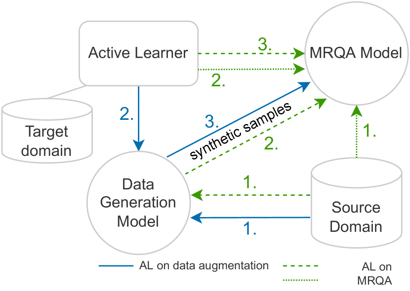
Figure 1: Three possible variants employing AL in our setup: our approach (solid blue) trains a data generation model on the source domain first (step 1), then applies AL on it (step 2) and generates synthetic data which are used to train the MRQA model (step 3). In contrast, the other possibilities (dashed and dotted green) apply AL directly to the MRQA model after previous fine-tuning with synthetic or source domain data. The target domain has only limited resources to annotate samples but contains many unlabelled documents.

Our novel approach to tackle MRQA in low-resource settings with minimal human input, is based on combining data generation with AL. In this section we describe the models involved, i.e. the data generation and the MRQA model, as well as our iterative sample selection, which adapts and combines various existing scores, with the addition of a novel one. A high-level overview of our approach is provided in figure 1.

3.1 Data Generation for MRQA

Model

Hereafter, we denote the question as $q$, the answer as $a$ and the corresponding context as $c$. Regarding data generation, we consider the QA2S model proposed by Shakeri et al. (2020), since this model shows best overall performance in their and our experiments. The considered model makes use of a pre-trained encoder-decoder LM and it is fine-tuned to generate the question given the context, followed by generating the answer given the context and the previously decoded question in a subsequent decoding step. Hence the same model is trained to approximate both probability distributions $p(a|q,c)$ and $p(q|c)$. Therefore, the question is generated in an auto-regressive manner and conditioned on the context:

$$p(q|c)=\sum\limits_{t=1}^{T}\log p(q_{t}|q_{<t},c).$$ (1)

Similarly, the answer is conditioned on the context and the question:

$$p(a|q,c)=\sum\limits_{t=1}^{T}\log p(a_{t}|a_{<t},q,c).$$ (2)

The pairs of special tokens <a>, </a> and <q>, </q> mark the answer and the question in the sequence, respectively. During inference, a two-step decoding process is used and <q> and <a> are given as begin-of-sequence tokens to start generating the question and the answer, respectively.

Decoding

Generating questions is performed by nucleus sampling (Holtzman et al., 2020) from the output distribution over the vocabulary, considering 95% of the probability mass and top 20 tokens in each step. The answer is then decoded greedily with a beam search of size 10. These hyperparameters were also used in prior work (Shakeri et al., 2020). Samples for which the answer does not occur in the context are discarded since we focus on extractive MRQA. Furthermore, only samples for which the corresponding end tokens are predicted correctly are considered as valid.

Filtering

Finally, only a subset of the generated samples is kept. Therefore, they are filtered using two sample filtering approaches, namely the LM score filtering, introduced by  Shakeri et al. (2020), and the round-trip consistency (RTcons) (Alberti et al., 2019). In LM score filtering, the generated samples are sorted according to the probability $p(y|y_{<t},x)$ as given by the generation model and the top $n$ samples are kept (we use $n=5$). Regarding the RTcons filtering, an MRQA model is used to assess the generated question-answer pair: The generated question along with the context is fed into an MRQA model to predict the answer. The sample is then discarded if the predicted answer does not match the generated one. Since RTcons might discard all samples generated from a context, we fine-tune the MRQA model (previously fine-tuned on the source domain) used for RTcons filtering also on the available samples from the target domain.

3.2 MRQA Model

We employ pre-trained BERT (Devlin et al., 2019) for encoding the question concatenated with the context. On top, a span extraction head models the probability for each context token to be the start and the end of the answer span. We refer to Devlin et al. (2019) for more details.

Algorithm 1 Model Training with AL

1:

2:data $\mathcal{D}_{\textrm{pool}}$, $\mathcal{D}_{\textrm{eval}}$

3:scoring function $f_{\textrm{score}}$

4:iterations $r$, number of samples $n$

5:Initialize models $\mathcal{M}_{\textrm{Gen}},\mathcal{M}_{\textrm{MRQA}}$ with pre-trained weights

6:$\mathcal{D}_{\textrm{train}}=\emptyset$

7:for $\textrm{iteration}=1,2,\ldots,r$ do

8:     $\mathcal{D}_{\textrm{selected}}\leftarrow$ select $n$ top scoring samples using $f_{\textrm{score}}$ and $\mathcal{M}_{\textrm{Gen}},\mathcal{M}_{\textrm{MRQA}}$ for labeling

9:     $\mathcal{D}_{\textrm{train}}\leftarrow\mathcal{D}_{\textrm{train}}\cup\mathcal{D}_{\textrm{selected}}$

10:     $\mathcal{D}_{\textrm{pool}}\leftarrow\mathcal{D}_{\textrm{pool}}\setminus\mathcal{D}_{\textrm{selected}}$

11:     Re-initialize models $\mathcal{M}_{\textrm{Gen}},\mathcal{M}_{\textrm{MRQA}}$ with pre-trained weights

12:     Fine-tune $\mathcal{M}_{\textrm{Gen}},\mathcal{M}_{\textrm{MRQA}}$ on $\mathcal{D}_{\textrm{train}}$ and load best models w.r.t. $\mathcal{D}_{\textrm{eval}}$ (using e.g. loss, F1)

13:end for

3.3 Active Learning

We consider different context scoring functions to be used in an AL scenario with pool based sampling for our specific task. We borrow Sentence Probability (SP), Dropout-based Sentence Probability (D-SP) and Dropout-based Lexical Similarity (LS) from unsupervised quality estimates (Fomicheva et al., 2020; Xiao et al., 2020) and adapt them as scoring functions in our setting. We also introduce round-trip scoring (RT), which incorporates the MRQA model in the sample selection process: We believe that, during data generation, it is important to link the sample selection process with the eventual downstream task, in order to generate high quality samples. Otherwise, the data generation model is not constrained in terms of questions being generated, potentially ending up generating questions which do not take the given context or evidence into account. Finally, we also compare scoring functions based on the data generation model with an approach that only uses the MRQA model. For this purpose, we consider Bayesian Active Learning by Disagreement (BALD) (Houlsby et al., 2011; Gal et al., 2017) as a baseline. In all cases, we initially fine-tune the models on the generic source domain in order to have a good starting point. Our novel approach, combining data generation together with AL, is briefly described in Algorithm 1.

3.3.1 Scoring functions

Sentence Probability (SP)

This scoring function is based on the probability distribution of the data generation model. The contexts are scored according to the sentence probability of the answer being generated:

$$\textrm{SP}(\theta)=\frac{1}{T}\sum\limits_{t=1}^{T}\log p(a_{t}|a_{<t},c,q,\theta).$$ (3)

We generate the question and answer by greedy decoding with beam search of size 10, but only use the produced answer for scoring a sample’s context.

Dropout-based Sentence Probability (D-SP)

In contrast to SP, D-SP makes use of multiple data generation models to compute the sentence probability:

$$\textrm{D-SP}=\frac{1}{N}\sum\limits_{n=1}^{N}\textrm{SP}(\theta_{n}).$$ (4)

We employ dropout at inference time (in addition to during fine-tuning) to realize different subsets of the model, as described by Gal and Ghahramani (2016), running $N$ forward passes. The output is decoded similarly to SP and the same prediction is used in all forward passes.

Dropout-based Lexical Similarity (LS)

Regarding LS, multiple answers are decoded using multiple models (again realized via dropout), and all of them are compared pairwise at the lexical level using the Meteor (Banerjee and Lavie, 2005) metric (with $i\neq j$):

$$\textrm{LS}=\frac{1}{N*(N-1)}\sum\limits_{i=1}^{N}\sum\limits_{j=1}^{N}\textrm{Meteor}(a_{i},a_{j}).$$ (5)

Decoding is again implemented greedily using beam search of size 10.

Since the ultimate goal is to improve the performance of the MRQA model, we propose the following novel methods integrating the MRQA model in the computation of the ranking scores:

Round-trip (RT)

We generate question-answer pairs from the context similarly to SP, and then we apply an MRQA model in order to rank the samples according to the F1 score between the predicted answer and the answer generated by the data generation model. We therefore prefer documents for which the data generation model will generate question-answer pairs which the MRQA model cannot predict correctly.

D-SP+RT

We combine the D-SP and the RT scores sample-wise to obtain the final ranking score. To this end, the D-SP score is rescaled so that its range matches the RT score (thus the best prediction corresponds to the value of 1.0) and the distribution is similar to RT and has been found using manual inspection of samples’ scores:

$$\textrm{D-SP+RT}=\exp(4\times\textrm{D-SP})^{2}+\textrm{RT}.$$ (6)

3.3.2 Scoring function for MRQA model

When only the MRQA model is considered, we use the BALD score (Houlsby et al., 2011) to measure the uncertainty of the model’s predictions, using entropy H given training data $\mathcal{D}$ and model weights $\theta$:

$$\textrm{H}[y|x,\mathcal{D}]-\mathbb{E}_{\theta\sim p(\theta|\mathcal{D})}\textrm{H}[y|x,\theta].$$ (7)

In order to make computation feasible, we calculate the BALD score (using dropout) independently for start and end probabilities. The sum of both scores is then used to rate and order the unlabeled samples.

4 Experimental Setup

We focus on the low-resource scenario, where we assume to be able to use an extremely small amount of annotated samples (200) from the target domain. In addition to a large annotated source domain, we assume to have many unlabeled documents available from the target domain as well, which can be used for generating new samples. We consider this assumption to be valid in general, as one of the main goals of MRQA is to provide better access to the vast amount of existing documents.

4.1 Data

We consider SQuAD as source domain and NaturalQuestions (NQ), TechQA and BioASQ as target domains; some statistics are summarized in table 1. The main reason for choosing these datasets is to consider examples of very specialized domains (TechQA, BioASQ) completely different from the source domain, as well as an example of a domain overlapping with the source domain (NQ). Since we focus on the low-resource setting, in absence of AL we randomly choose 200 samples from the training data of the target domain. In case of AL, samples from the target domain are collected as described in section §4.4. Further details on the datasets can be found in the appendix.

Domain	Context tokens			Questions tokens			Answer tokens
	Min	Max	Mean	Min	Max	Mean	Min	Max	Mean
SQuAD	25	853	155.75	1	61	12.29	1	68	4.23
NQ	10	3143	245.4	7	29	9.76	1	270	5.25
TechQA	38	38925	1484.08	6	561	69.37	5	545	98.76
BioASQ	27	960	337.71	5	36	15.06	1	76	4.42

Table 1: Statistics about the train split for each domain obtained with the BERT tokenizer.

4.2 Question & Answer Generation

Training

Similarly to Shakeri et al. (2020), in our approach we use bart-large (Lewis et al., 2019) with 406M parameters for the data generation model as this showed better results in our preliminary experiments compared to gpt2-large (Radford et al., 2019). It is fine-tuned using cross entropy loss and the model with the best loss on the evaluation data is selected. Fine-tuning of the data generation model is performed for 5 epochs on source domain data first, followed by fine-tuning on the target domain. As we found that 5 epochs is too few for fine-tuning in the low-resource setting, on the target domain we fine-tune it for 10 epochs instead. In addition, we perform early stopping based on the dev set loss.

To fit the context concatenated with the question into the model we split the context into several chunks. We only consider those chunks where the answer does occur in the context. Additionally, since TechQA has long questions we truncate the questions to the first 200 tokens, to allow for sufficient space in the input for the context as well.

Synthetic Data Generation

Regarding question generation (i.e. the first decoding step), we allow contexts to have a size of up to 724 tokens; this allows the generated questions to be composed of up to 300 tokens, as both will be fed into the model in the second decoding step and their sum cannot exceed the total of 1024 tokens (including special tokens). Chunking this input would be difficult, since aggregating the generated text is not simple (especially if outputs do not overlap). We generate 10 questions per input, followed by one answer for each question-context pair, yielding up to 10 samples per context. In total we choose 100000 documents from the target domain, ignoring contexts with less than 100 tokens. Regarding the NQ dataset, this is the reason why only 50535 documents are considered.

4.3 MRQA Model

We use bert-base-uncased (Devlin et al., 2019) in the MRQA model for comparability with prior work, with a maximum input length of 512 tokens and a stride of 128. Similarly as for the data generation model, when considering the TechQA dataset we truncate the questions (whether from the train/dev corpus or synthetically generated). Since chunking is applied to the inputs and predictions are aggregated afterwards (by choosing the best span over all chunks’ predictions), it may happen that the answer of a sample is not completely included in a chunk’s context. We especially observe this for TechQA, where the performance on the evaluation data is greatly degraded as the model never has the chance to predict the answer correctly for some samples.

4.4 Active Learning

In the scenarios with AL, we score available samples using each of the scoring functions described in Section 3.3, running 10 forward passes for D-SP, LS, D-SP+RT and BALD. Available samples include only samples with labels since we simulate the domain expert. We run 4 iterations, starting initially with all available samples from the target domain in the pool, and then at each step selecting the 50 samples the model is least confident about. In each iteration we remove the selected samples from the query pool and fine-tune the models on all samples selected so far, always initializing the model with weights gained when fine-tuned on the source domain (or on the synthetic data for MRQA) in order to not introduce any biases. Since D-SP, LS and RT are computationally expensive, with LS actually decoding generated text after each forward pass, performing AL with LS, RT and D-SP+RT on NQ was not feasible for us. Therefore, we selected 10000 random samples from this domain for use with AL, denoted as NQ#10000 in our experiments.

4.5 Baselines

In order to assess the performance of our approach we compare it against several baselines. Firstly, we consider an MRQA model fine-tuned on the target domain data only. Then, we fine-tune a second MRQA model on SQuAD first, followed by further fine-tuning on samples from the target domain. In order to determine which scenario benefits from AL the most, we perform AL on the MRQA model with BALD. Prior to applying AL, one MRQA model is fine-tuned on SQuAD while a separate MRQA model is fine-tuned on synthetic data generated using the data generation model fine-tuned on SQuAD.

5 Experimental Results

We assess the performance of the MRQA models using exact match (EM) and F1 score of the answers at the token level.

Model	NQ		NQ#10000		TechQA		BioASQ
	EM	F1	EM	F1	EM	F1	EM	F1
MRQA only
target domain (random subset)	20.61 $\pm$ 1.01	29.28 $\pm$ 0.86	20.61 $\pm$ 1.01	29.28 $\pm$ 0.86	24.75 $\pm$ 1.02	53.81 $\pm$ 0.68	39.93 $\pm$ 1.46	46.52 $\pm$ 1.67
SQuAD + target domain (random subset)	49.26 $\pm$ 0.23	62.72 $\pm$ 0.3	49.26 $\pm$ 0.23	62.72 $\pm$ 0.3	27.75 $\pm$ 0.64	56.19 $\pm$ 0.89	67.31 $\pm$ 0.72	73.96 $\pm$ 0.32
SQuAD + target domain (BALD)	48.61 $\pm$ 0.84	63.28 $\pm$ 0.68	49.78 $\pm$ 0.45	64.12 $\pm$ 0.42	27 $\pm$ 0.47	53.89 $\pm$ 0.96	65.58 $\pm$ 1.16	74.69 $\pm$ 1.23
Synthetic data generation
SQuAD	51.37 †	64.38 †	51.37 †	64.38 †	0.63 ∗	19.76 ∗	50.5 ∗	62.99 ∗
SQuAD + BALD	52.53 $\pm$ 0.44 †	66.18 $\pm$ 0.36 †	53.10 $\pm$ 0.47 ∗	66.58 $\pm$ 0.42 ∗	27.88 $\pm$ 1.29 †	57.04 $\pm$ 0.93 †	68.7 $\pm$ 1.02 ∗	77.44 $\pm$ 0.53 ∗
Our proposed AL framework
a) random	54.61 $\pm$ 0.15 ∗	67.13 $\pm$ 0.15 ∗	54.61 $\pm$ 0.15 ∗	67.13 $\pm$ 0.15 ∗	30.63 $\pm$ 0.83 ∗	57.04 $\pm$ 1.24 ∗	72.36 $\pm$ 0.95 ∗	80.15 $\pm$ 0.85 ∗
b) SP	54.48 $\pm$ 0.02 †	67.23 $\pm$ 0 †	55.39 $\pm$ 0.07 †	68.04 $\pm$ 0.07 †	30.38 $\pm$ 0.85 ∗	56.51 $\pm$ 0.73 ∗	72.03 $\pm$ 0.77 ∗	80.63 $\pm$ 0.59 ∗
c) D-SP	54.8 $\pm$ 0.16 †	67.68 $\pm$ 0.11 †	55.11 $\pm$ 0.08 ∗	67.86 $\pm$ 0.08 ∗	32.5 $\pm$ 0.56 †	56.17 $\pm$ 0.41 †	75.35 $\pm$ 0.64 ∗	82.57 $\pm$ 0.52 ∗
d) LS	-	-	54.83 $\pm$ 0.19 ∗	67.75 $\pm$ 0.16 ∗	31.25 $\pm$ 1.25 †	55.5 $\pm$ 1.39 †	71.89 $\pm$ 0.72 †	79.95 $\pm$ 0.53 †
e) RT	-	-	55.43 $\pm$ 0.05 ∗	68.28 $\pm$ 0.08 ∗	32 $\pm$ 0.47 †	58.89 $\pm$ 0.62 †	71.96 $\pm$ 0.16 ∗	80.23 $\pm$ 0.44 ∗
f) D-SP+RT	-	-	55.55 $\pm$ 0.14 ∗	67.77 $\pm$ 0.15 ∗	30.75 $\pm$ 0.73 †	57.81 $\pm$ 0.36 †	71.69 $\pm$ 1.08 ∗	78.77 $\pm$ 1.13 ∗
Full target domain (MRQA only)	66.63	78.64	66.63	78.64	26.88	55.9	78.07	80.64

Table 2: EM and F1 scores (with std. dev. calculated over 5 MRQA model runs) obtained by MRQA models considering only 200 annotated samples from the target domains (but the last row which considers all samples from the target domain). Only results from the best filtering strategy (for synthetic data) for each model according to the F1 metric are shown (^∗ for LM filtering, ^† for RTcons filtering). Regarding the first 2 baselines, the 200 samples are randomly drawn from the target domain. For our approach, the data generation model is fine-tuned on SQuAD first and afterwards 4 iterations of AL are run, each querying for 50 samples to annotate. Following that, an MRQA model is fine-tuned on the filtered synthetic data and further fine-tuned using the annotated samples. AL improves results for all domains; best overall results are highlighted in bold.

5.1 AL in Multiple Stages

We report results of our experiments in table 2. In our scenario, AL performs better than random sampling, both when it is applied on the MRQA model and when it is applied on the data generation model as well, as the results obtained with our various scoring functions demonstrate. Without AL, we get the best results for our low-resource setting on all datasets when the data generation model fine-tuned on both SQuAD and the target domain data is employed for data augmentation. In terms of F1 metric, we get 67.13% on NQ, 57.04% on TechQA and 80.15% on BioASQ.

We also observe that AL improves performance on all domains, with an absolute increase of F1 of 0.55% (NQ), 1.15% (NQ#10000), 1.85% (TechQA) and 2.42% (BioASQ). Performance on NQ is in general not improved much when including additional data from the target domain, probably because of its similarity with the source domain (SQuAD) w.r.t. the others. Although fine-tuning the data generation model on target domain data gives already superior results w.r.t. BALD, applying AL at the MRQA model still improves performance on all datasets, if compared to simply fine-tuning the MRQA model on SQuAD and random target domain data. In general, we find that target domain data is necessary when tackling more specialized domains, as in the case of TechQA and BioASQ, as this improves F1 by up to 39.13% and 19.58%, respectively, with only 200 samples annotated.

5.2 Scoring functions for data generation

Regarding the scoring functions, in our experiments we observe that RT, D-SP and its combination D-SP+RT work best w.r.t. the others. While RT yields high F1 scores for NQ#10000 (68.28%) and TechQA (58.89%), BioASQ profits the most from D-SP (82.57%) with the latter two domains actually outperforming the case where all target domain samples are annotated.

In addition, we do not observe any degradation of performance when subsampling NQ. Therefore, subsampling large pools of (unlabeled) samples for better efficiency seems to be a valid choice when applying AL.

6 Discussion

6.1 Insights about drawn samples

To better understand the performance of the considered AL methods, we analyze different aspects of the samples which are selected for labeling.

Statistics on drawn samples

	$\varnothing$ context length (rc / qa2s)	$\varnothing$ question length (rc / qa2s)
BALD	1462.45 / 1521.82	60.43 / 67.94
SP	2564.99 / 2715.05	71.65 / 83.34
LS	2519.89 / 2660.34	69.98 / 77.63
RT	1836.84 / 1950.62	75.98 / 81.28
D-SP+RT	2518.53 / 2668.70	66.78 / 75.84
D-SP	2531.28 / 2686.99	69.32 / 80.47
RANDOM	1588.09 / 1668.24	67.79 / 74.43

Table 3: Context and question length in tokens for BERT and BART tokenization on TechQA comparing the sample selection methods: AL methods at the data generation stage prefer samples with long contexts.

Applying AL on the data generation model selects samples with long contexts for all domains. Exemplary statistics are shown in table 3 for TechQA. RT selects samples with long contexts. Still, they are in average much shorter then for the other AL scoring functions for the data generation model. Furthermore, AL on the MRQA model (BALD) does not put emphasis on it which can further explain the improvements of applying AL at the stage of data generation. For statistics on all domains see the appendix.

Overlap of drawn samples

	BALD	SP	LS	RT	D-SP+RT	D-SP	Random
BALD	200	39	44	42	54	49	42
SP	39	200	49	49	66	72	40
LS	44	49	200	37	48	46	41
RT	42	49	37	200	63	49	15
D-SP+RT	54	66	48	63	200	82	42
D-SP	49	72	46	49	82	200	36
Random	42	40	41	15	42	36	200

Table 4: Overlap of samples for the various AL approaches on BioASQ: The overlap of the scoring functions is rather small.

We analyze the overlap of the chosen samples between the different AL strategies. Table 4 reflects this for the BioASQ domain. We observe rather small sample overlap among the approaches, a trend that holds for the other domains as well. The overlap depends on the dataset with larger datasets having less overlap.

Distribution of scores

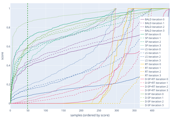
Figure 2: Sample score distribution for TechQA: RT scores many samples low, but surprisingly also rates some samples as best, although the task of predicting the generated answer for a generated question is complex. Scores have been rescaled to $\left[0,1\right]$.

Figure 2 shows the distribution of scores over all available samples in each iteration of AL for the TechQA dataset. Regarding RT scoring, we observe a steep curve where, depending on the dataset, many samples are rated as 0 and many as 1. This indicates that both models, data generation and MRQA, work very well in combination since well working samples are rated high. The RT scoring seems to be also a good measure to quantify the “difference” between the target domain and the source domain. For example, for both NQ and BioASQ, RT scores are much better than those for TechQA. This happens probably because the RT scoring method considers the downstream MRQA task when computing the score thus reflecting the larger distribution shift when more specialized domains are considered. Therefore, for the TechQA dataset, the visualization suggests that one might as well select all 200 samples in one iteration, instead of annotating 50 samples in four consecutive iterations. Another interesting behavior we observe is that the RT method scores samples best in the first iteration. This might occur due to potential overfitting of the data generation model, being fine-tuned with 50 samples from the target domain, resulting in a decrease of score in the following iteration.

Distribution of samples

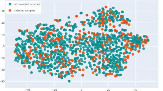
Figure 3: Visualization of the BioASQ dataset samples using representations retrieved using the MRQA model, with samples selected by RT in the last iteration (221 instances) marked red.

In order for the MRQA model to perform well, it is important that a set of diverse samples is selected by the AL strategy. Figure 3 shows a visualization, based on t-SNE, of the diversity of samples drawn from the BioASQ dataset according to RT scoring in the last iteration. More examples can be found in the appendix.

6.2 Lessons Learned

For all domains, applying AL improves the MRQA task, especially when it is applied at the data generation stage. Furthermore, our proposed method - RT scoring - provides a competitive scoring function. F1 scores are consistently increased by 1.15% (NQ#10000), 1.85% (TechQA) and 2.42% (BioASQ). We expect that this improvement could be further increased when more diverse (unlabeled) samples are available for querying. This can thus be used as an approach to minimize the costly annotation effort when targeting specialized domains.

When a small amount of labeled samples from the target domain exists, generating synthetic data to augment the training set is a robust solution. However, if possible, AL should be used at the stage of data generation, thus incorporating humans early in the process, as our findings from AL on the data generation model in contrast to AL on the MRQA model demonstrate.

7 Conclusion

Although data scarcity is ubiquitous in practice, there is a lack of approaches that address this issue for the MRQA task in specialized domains. Therefore, appropriate methods applicable to realistic low-resource domains are of great importance since deep learning models usually work well when plenty of annotated, in-domain samples are available. In our work, we showed how to utilize Active Learning to boost performance when addressing the challenging MRQA problem in low-resource, domain-specific scenarios relevant in practice. To this end, we introduced a novel approach that combines data generation with AL to tackle the MRQA problem, resulting in a boost in performance with low labeling effort. We further analyzed performance of AL when applied to the MRQA model directly in comparison to when applied to the data generation process, showing evidenced improvements of predictive performance in the latter scenario, especially when using our newly introduced scoring function tailored to the MRQA task.

Limitations

Due to a lack of resources, we were not able to conduct experiments varying the amount of iterations in case of AL or the number of annotated samples.

Furthermore, the results shown in this paper may not be effortlessly transferable to all domains, like e.g. in different languages, although the described setup could be adapted. Also, there is a chance that a domain we did not consider behaves completely different due to its characteristics, which might not be obvious before testing it in our setup.

Lastly, we should mention that fine-tuning the data generation model followed by generating plenty of synthetic data and MRQA model training requires significant amount of computing time and resources.

Appendix A Data

SQuAD

We consider the official SQuAD 1.1 dataset (Rajpurkar et al., 2016) and its split in training and development (dev) sets comprised of 87599 and and 10570 samples, respectively. We use SQuAD as source domain for fine-tuning the data generation model and for fine-tuning the MRQA model in addition to target domain data without data generation.

NaturalQuestions

We use the NaturalQuestions dataset (Kwiatkowski et al., 2019), preprocessed for the MRQA Shared Task 2019 (Fisch et al., 2019). The train split contains 104071 samples, while the dev split has 12836 samples. In our work, this dataset was chosen due to its domain being similar to SQuAD. The documents from the training set are used to generate question-answer pairs, while documents from the dev set are excluded.

TechQA

TechQA is a dataset released by IBM (Castelli et al., 2019). Questions are asked in forum post-style and the answer is given as spans within technotes (i.e. the documents). The dataset contains 600 training samples, including unanswerable questions. In our work we only consider the answerable subset of 450 questions. The official dev data with 160 answerable samples was used for evaluation, since the test set is kept secret to ensure integrity of the benchmark. Passages from the corpus of technotes containing 800K+ documents were used to generate data.

BioASQ

Regarding the BioASQ dataset (Tsatsaronis et al., 2015), we rely on the version preprocessed for the MRQA Shared Task 2019 (Fisch et al., 2019). It includes a dev set with 1504 samples. We create random splits for training, development and testing with 70%, 20% and 10% of samples, respectively. For the data generation process, we crawl PubMed abstracts as unlabeled documents.

Appendix B Implementation Details

In our implementation we rely on PyTorch (Paszke et al., 2017) and the transformers library (Wolf et al., 2020) for the models, as well as for training. The datasets library (Lhoest et al., 2021) is used for loading and preprocessing data.

B.1 Hyperparameters

The MRQA model, as well as the data generation model, have been both trained with Adam Optimizer (Kingma and Ba, 2017), a learning rate of $3\mathrm{e}{-5}$ and a batch size of $24$. Warm-up was set to $10\%$ for fine-tuning the data generation model, while it was disabled for fine-tuning the MRQA model. Similarly to the models used for the downstream MRQA task, bert-base-uncased was used for RTcons filtering.

MRQA model fine-tuning turned out to be quite fluctuating in terms of the evaluation score. Therefore, we performed a hyperparameter search including learning rate, warm-up steps (using linear scheduler), L2 regularization, pre-trained weight decay for the encoder and for the output layer separately, freezing the encoder or its embedding, training of only top-n layers and re-initializing top-n layers. As a result of manual tuning, only pre-trained weight decay on the encoder with $\lambda=1\mathrm{e}{-7}$ was employed, while all layers were fine-tuned without re-initialization.

Appendix C Computational Resources

All our models were run on RTX A6000 48GB, RTX 3090 24GB or GTX Titan X 12GB graphics cards. This includes training, evaluation, inference (for RTcons filtering and RT scoring) of models and generation of synthetic samples.

Appendix D Further Analysis

	# samples	# unique contexts	$\varnothing$ context length (rc / qa2s)	$\varnothing$ question length (rc / qa2s)	# instances (rc / qa2s)
BALD	200	194	317.32 / 318.03	9.62 / 10.51	269 / 402
SP	200	161	1427.68 / 1475.08	9.42 / 10.26	807 / 439
D-SP	200	181	1016.62 / 1040.51	9.60 / 10.37	619 / 411
RANDOM	200	200	216.43 / 219.00	9.95 / 10.77	240 / 400

(a) NQ

	# samples	# unique contexts	$\varnothing$ context length (rc / qa2s)	$\varnothing$ question length (rc / qa2s)	# instances (rc / qa2s)
BALD	200	200	391.49 / 388.62	9.67 / 10.54	311 / 406
SP	200	185	1295.74 / 1330.08	9.76 / 10.69	746 / 424
LS	200	199	600.48 / 607.56	9.96 / 10.53	403 / 404
RT	200	197	645.59 / 658.51	9.82 / 10.62	436 / 410
D-SP+RT	200	195	1068.60 / 1087.87	9.82 / 10.68	643 / 420
D-SP	200	192	1087.01 / 1109.31	9.71 / 10.61	654 / 422
RANDOM	200	200	216.43 / 219.00	9.95 / 10.77	240 / 400

(b) NQ#10000

	# samples	# unique contexts	$\varnothing$ context length (rc / qa2s)	$\varnothing$ question length (rc / qa2s)	# instances (rc / qa2s)
BALD	200	177	1462.45 / 1521.82	60.43 / 67.94	909 / 404
SP	200	175	2564.99 / 2715.05	71.65 / 83.34	1635 / 409
LS	200	177	2519.89 / 2660.34	69.98 / 77.63	1597 / 408
RT	200	182	1836.84 / 1950.62	75.98 / 81.28	1185 / 410
D-SP+RT	200	181	2518.53 / 2668.70	66.78 / 75.84	1595 / 406
D-SP	200	176	2531.28 / 2686.99	69.32 / 80.47	1614 / 406
RANDOM	200	182	1588.09 / 1668.24	67.79 / 74.43	1034 / 402

(c) TechQA

	# samples	# unique contexts	$\varnothing$ context length (rc / qa2s)	$\varnothing$ question length (rc / qa2s)	# instances (rc / qa2s)
BALD	200	199	384.64 / 374.82	15.17 / 14.91	236 / 400
SP	200	200	357.19 / 344.81	15.60 / 15.46	225 / 400
LS	200	200	341.46 / 329.62	15.62 / 15.45	220 / 400
RT	200	199	344.85 / 334.69	14.66 / 14.43	221 / 400
D-SP+RT	200	197	338.15 / 328.59	14.98 / 14.69	222 / 400
D-SP	200	199	348.22 / 336.84	14.88 / 14.70	227 / 400
RANDOM	200	199	339.80 / 328.79	15.20 / 15.04	216 / 400

(d) BioASQ

Table 5: Statistics for the various domains when performing data generation with lengths measured in tokens using the corresponding tokenizer: AL methods on the data generation model prefer samples with long contexts with RT putting less emphasis on it.

	BALD	SP	D-SP	Random
BALD	200	0	0	0
SP	0	200	2	1
D-SP	0	2	200	0
Random	0	1	0	200

(a) NQ

	BALD	SP	LS	RT	D-SP+RT	D-SP	Random
BALD	200	8	11	3	8	6	0
SP	8	200	20	18	38	42	6
LS	11	20	200	7	20	21	5
RT	3	18	7	200	17	10	0
D-SP+RT	8	38	20	17	200	70	3
D-SP	6	42	21	10	70	200	5
Random	0	6	5	0	3	5	200

(b) NQ#10000

	BALD	SP	LS	RT	D-SP+RT	D-SP	Random
BALD	200	95	88	86	88	87	96
SP	95	200	129	103	133	134	93
LS	88	129	200	99	116	111	85
RT	86	103	99	200	106	101	58
D-SP+RT	88	133	116	106	200	135	82
D-SP	87	134	111	101	135	200	88
Random	96	93	85	58	82	88	200

(c) TechQA

	BALD	SP	LS	RT	D-SP+RT	D-SP	Random
BALD	200	39	44	42	54	49	42
SP	39	200	49	49	66	72	40
LS	44	49	200	37	48	46	41
RT	42	49	37	200	63	49	15
D-SP+RT	54	66	48	63	200	82	42
D-SP	49	72	46	49	82	200	36
Random	42	40	41	15	42	36	200

(d) BioASQ

Table 6: Overlap for the domains. Although the overlap is quite high for TechQA, we explain this with the small amount of total samples available. In contrast, we see a small overlap for large datasets, like NQ.

Tables 5 and 6 show the statistics and sample overlap for all domains.

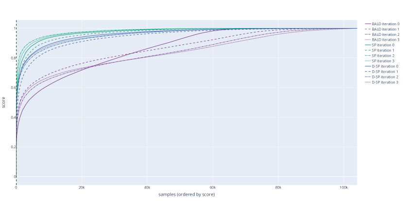
Figure 4: Sample score distribution for NQ. Scores have been rescaled to $\left[0,1\right]$.

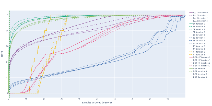
Figure 5: Sample score distribution for NQ#10000. Scores have been rescaled to $\left[0,1\right]$.

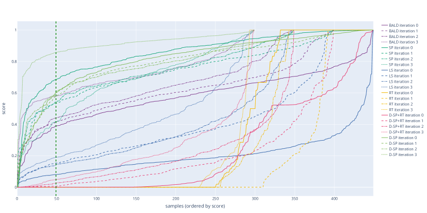
Figure 6: Sample score distribution for TechQA. Scores have been rescaled to $\left[0,1\right]$.

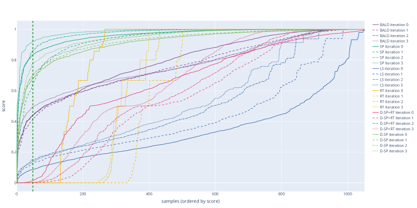
Figure 7: Sample score distribution for BioASQ. Scores have been rescaled to $\left[0,1\right]$.

Figures 4, 5, 6 and 7 show the distribution of scores over all queryable samples in each iteration of AL for the different datasets.

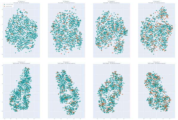
Figure 8: Visualization of sample encoding distribution on BioASQ with RT scoring on both models, MRQA as well as data generation, via t-SNE of the last layer hidden states; sentence representation by averaging over tokens.

Figure 8 shows the sample distribution for BioASQ using RT scoring for AL.

References

- Alberti et al. (2019) Chris Alberti, Daniel Andor, Emily Pitler, Jacob Devlin, and Michael Collins. 2019. Synthetic QA Corpora Generation with Roundtrip Consistency. arXiv:1906.05416 [cs]. ArXiv: 1906.05416.
- Banerjee and Lavie (2005) Satanjeev Banerjee and Alon Lavie. 2005. METEOR: An Automatic Metric for MT Evaluation with Improved Correlation with Human Judgments. In Proceedings of the ACL Workshop on Intrinsic and Extrinsic Evaluation Measures for Machine Translation and/or Summarization, pages 65–72, Ann Arbor, Michigan. Association for Computational Linguistics.
- Castelli et al. (2019) Vittorio Castelli, Rishav Chakravarti, Saswati Dana, Anthony Ferritto, Radu Florian, Martin Franz, Dinesh Garg, Dinesh Khandelwal, Scott McCarley, Mike McCawley, Mohamed Nasr, Lin Pan, Cezar Pendus, John Pitrelli, Saurabh Pujar, Salim Roukos, Andrzej Sakrajda, Avirup Sil, Rosario Uceda-Sosa, Todd Ward, and Rong Zhang. 2019. The TechQA Dataset. arXiv:1911.02984 [cs]. ArXiv: 1911.02984.
- Chang et al. (2020) Haw-Shiuan Chang, Shankar Vembu, Sunil Mohan, Rheeya Uppaal, and Andrew McCallum. 2020. Using Error Decay Prediction to Overcome Practical Issues of Deep Active Learning for Named Entity Recognition. Machine Learning, 109(9-10):1749–1778. ArXiv: 1911.07335.
- Chen et al. (2020) Yu Chen, Lingfei Wu, and Mohammed J. Zaki. 2020. Reinforcement Learning Based Graph-to-Sequence Model for Natural Question Generation. arXiv:1908.04942 [cs]. ArXiv: 1908.04942.
- Cohn et al. (1996) D. A. Cohn, Z. Ghahramani, and M. I. Jordan. 1996. Active Learning with Statistical Models. arXiv:cs/9603104. ArXiv: cs/9603104.
- Devlin et al. (2019) Jacob Devlin, Ming-Wei Chang, Kenton Lee, and Kristina Toutanova. 2019. BERT: Pre-training of Deep Bidirectional Transformers for Language Understanding. arXiv:1810.04805 [cs]. ArXiv: 1810.04805.
- Du et al. (2017) Xinya Du, Junru Shao, and Claire Cardie. 2017. Learning to Ask: Neural Question Generation for Reading Comprehension. arXiv:1705.00106 [cs]. ArXiv: 1705.00106.
- Duan et al. (2017) Nan Duan, Duyu Tang, Peng Chen, and Ming Zhou. 2017. Question Generation for Question Answering. In Proceedings of the 2017 Conference on Empirical Methods in Natural Language Processing, pages 866–874, Copenhagen, Denmark. Association for Computational Linguistics.
- Fang et al. (2017) Meng Fang, Yuan Li, and Trevor Cohn. 2017. Learning how to Active Learn: A Deep Reinforcement Learning Approach. arXiv:1708.02383 [cs]. ArXiv: 1708.02383.
- Fisch et al. (2019) Adam Fisch, Alon Talmor, Robin Jia, Minjoon Seo, Eunsol Choi, and Danqi Chen. 2019. MRQA 2019 Shared Task: Evaluating Generalization in Reading Comprehension. arXiv:1910.09753 [cs]. ArXiv: 1910.09753.
- Fomicheva et al. (2020) Marina Fomicheva, Shuo Sun, Lisa Yankovskaya, Frédéric Blain, Francisco Guzmán, Mark Fishel, Nikolaos Aletras, Vishrav Chaudhary, and Lucia Specia. 2020. Unsupervised Quality Estimation for Neural Machine Translation. arXiv:2005.10608 [cs]. ArXiv: 2005.10608.
- Gal and Ghahramani (2016) Yarin Gal and Zoubin Ghahramani. 2016. Dropout as a Bayesian Approximation: Representing Model Uncertainty in Deep Learning. arXiv:1506.02142 [cs, stat]. ArXiv: 1506.02142.
- Gal et al. (2017) Yarin Gal, Riashat Islam, and Zoubin Ghahramani. 2017. Deep Bayesian Active Learning with Image Data. arXiv:1703.02910 [cs, stat]. ArXiv: 1703.02910.
- Hedderich et al. (2021) Michael A. Hedderich, Lukas Lange, Heike Adel, Jannik Strötgen, and Dietrich Klakow. 2021. A Survey on Recent Approaches for Natural Language Processing in Low-Resource Scenarios. arXiv:2010.12309 [cs]. ArXiv: 2010.12309.
- Holtzman et al. (2020) Ari Holtzman, Jan Buys, Li Du, Maxwell Forbes, and Yejin Choi. 2020. The Curious Case of Neural Text Degeneration. arXiv:1904.09751 [cs]. ArXiv: 1904.09751.
- Hong et al. (2019) Yining Hong, Jialu Wang, Yuting Jia, Weinan Zhang, and Xinbing Wang. 2019. Academic Reader: An Interactive Question Answering System on Academic Literatures. Proceedings of the AAAI Conference on Artificial Intelligence, 33(01):9855–9856. Number: 01.
- Houlsby et al. (2011) Neil Houlsby, Ferenc Huszár, Zoubin Ghahramani, and Máté Lengyel. 2011. Bayesian Active Learning for Classification and Preference Learning. arXiv:1112.5745 [cs, stat]. ArXiv: 1112.5745.
- Kingma and Ba (2017) Diederik P. Kingma and Jimmy Ba. 2017. Adam: A Method for Stochastic Optimization. arXiv:1412.6980 [cs]. ArXiv: 1412.6980.
- Klein and Nabi (2019) Tassilo Klein and Moin Nabi. 2019. Learning to Answer by Learning to Ask: Getting the Best of GPT-2 and BERT Worlds. arXiv:1911.02365 [cs]. ArXiv: 1911.02365.
- Kratzwald et al. (2020) Bernhard Kratzwald, Stefan Feuerriegel, and Huan Sun. 2020. Learning a Cost-Effective Annotation Policy for Question Answering. arXiv:2010.03476 [cs]. ArXiv: 2010.03476.
- Kwiatkowski et al. (2019) Tom Kwiatkowski, Jennimaria Palomaki, Olivia Redfield, Michael Collins, Ankur Parikh, Chris Alberti, Danielle Epstein, Illia Polosukhin, Matthew Kelcey, Jacob Devlin, Kenton Lee, Kristina N. Toutanova, Llion Jones, Ming-Wei Chang, Andrew Dai, Jakob Uszkoreit, Quoc Le, and Slav Petrov. 2019. Natural Questions: a Benchmark for Question Answering Research. Transactions of the Association of Computational Linguistics.
- Lee et al. (2020) Dong Bok Lee, Seanie Lee, Woo Tae Jeong, Donghwan Kim, and Sung Ju Hwang. 2020. Generating Diverse and Consistent QA pairs from Contexts with Information-Maximizing Hierarchical Conditional VAEs. arXiv:2005.13837 [cs]. ArXiv: 2005.13837.
- Lee et al. (2019) Seanie Lee, Donggyu Kim, and Jangwon Park. 2019. Domain-agnostic Question-Answering with Adversarial Training. arXiv:1910.09342 [cs]. ArXiv: 1910.09342.
- Lewis et al. (2019) Mike Lewis, Yinhan Liu, Naman Goyal, Marjan Ghazvininejad, Abdelrahman Mohamed, Omer Levy, Ves Stoyanov, and Luke Zettlemoyer. 2019. BART: Denoising Sequence-to-Sequence Pre-training for Natural Language Generation, Translation, and Comprehension. arXiv:1910.13461 [cs, stat]. ArXiv: 1910.13461.
- Lhoest et al. (2021) Quentin Lhoest, Albert Villanova del Moral, Patrick von Platen, Thomas Wolf, Yacine Jernite, Abhishek Thakur, Lewis Tunstall, Suraj Patil, Mariama Drame, Julien Chaumond, Julien Plu, Joe Davison, Simon Brandeis, Teven Le Scao, Victor Sanh, Kevin Canwen Xu, Nicolas Patry, Angelina McMillan-Major, Philipp Schmid, Sylvain Gugger, Steven Liu, Sylvain Lesage, Lysandre Debut, Théo Matussière, Clément Delangue, and Stas Bekman. 2021. huggingface/datasets: 1.11.0.
- Lin and Parikh (2017) Xiao Lin and Devi Parikh. 2017. Active Learning for Visual Question Answering: An Empirical Study. arXiv:1711.01732 [cs]. ArXiv: 1711.01732.
- Liu et al. (2020) Bang Liu, Haojie Wei, Di Niu, Haolan Chen, and Yancheng He. 2020. Asking Questions the Human Way: Scalable Question-Answer Generation from Text Corpus. Proceedings of The Web Conference 2020, pages 2032–2043. ArXiv: 2002.00748.
- Lowell et al. (2019) David Lowell, Zachary C. Lipton, and Byron C. Wallace. 2019. Practical Obstacles to Deploying Active Learning. arXiv:1807.04801 [cs, stat]. ArXiv: 1807.04801.
- Luo et al. (2021) Hongyin Luo, Shang-Wen Li, Seunghak Yu, and James Glass. 2021. Cooperative Learning of Zero-Shot Machine Reading Comprehension. arXiv:2103.07449 [cs]. ArXiv: 2103.07449.
- Ma et al. (2020) Xiyao Ma, Qile Zhu, Yanlin Zhou, Xiaolin Li, and Dapeng Wu. 2020. Improving Question Generation with Sentence-level Semantic Matching and Answer Position Inferring. arXiv:1912.00879 [cs]. ArXiv: 1912.00879.
- Mitkov and Ha (2003) Ruslan Mitkov and Le An Ha. 2003. Computer-aided generation of multiple-choice tests. In Proceedings of the HLT-NAACL 03 workshop on Building educational applications using natural language processing - Volume 2, HLT-NAACL-EDUC ’03, pages 17–22, USA. Association for Computational Linguistics.
- Nishida et al. (2020) Kosuke Nishida, Kyosuke Nishida, Itsumi Saito, Hisako Asano, and Junji Tomita. 2020. Unsupervised Domain Adaptation of Language Models for Reading Comprehension. arXiv:1911.10768 [cs]. ArXiv: 1911.10768.
- Paszke et al. (2017) Adam Paszke, Sam Gross, Soumith Chintala, Gregory Chanan, Edward Yang, Zachary DeVito, Zeming Lin, Alban Desmaison, Luca Antiga, and Adam Lerer. 2017. Automatic differentiation in PyTorch.
- Puri et al. (2020) Raul Puri, Ryan Spring, Mostofa Patwary, Mohammad Shoeybi, and Bryan Catanzaro. 2020. Training Question Answering Models From Synthetic Data. arXiv:2002.09599 [cs]. ArXiv: 2002.09599.
- Radford et al. (2019) Alec Radford, Jeff Wu, R. Child, David Luan, Dario Amodei, and Ilya Sutskever. 2019. Language Models are Unsupervised Multitask Learners. undefined.
- Rajpurkar et al. (2016) Pranav Rajpurkar, Jian Zhang, Konstantin Lopyrev, and Percy Liang. 2016. SQuAD: 100,000+ Questions for Machine Comprehension of Text. arXiv:1606.05250 [cs]. ArXiv: 1606.05250.
- Sachan and Xing (2018) Mrinmaya Sachan and Eric Xing. 2018. Self-Training for Jointly Learning to Ask and Answer Questions. In Proceedings of the 2018 Conference of the North American Chapter of the Association for Computational Linguistics: Human Language Technologies, Volume 1 (Long Papers), pages 629–640, New Orleans, Louisiana. Association for Computational Linguistics.
- Settles (2012) B. Settles. 2012. Active Learning. Synthesis Lectures on Artificial Intelligence and Machine Learning Series. Morgan & Claypool.
- Shakeri et al. (2020) Siamak Shakeri, Cicero Nogueira dos Santos, Henry Zhu, Patrick Ng, Feng Nan, Zhiguo Wang, Ramesh Nallapati, and Bing Xiang. 2020. End-to-End Synthetic Data Generation for Domain Adaptation of Question Answering Systems. arXiv:2010.06028 [cs]. ArXiv: 2010.06028.
- Siddhant and Lipton (2018) Aditya Siddhant and Zachary C. Lipton. 2018. Deep Bayesian Active Learning for Natural Language Processing: Results of a Large-Scale Empirical Study. arXiv:1808.05697 [cs, stat]. ArXiv: 1808.05697.
- Song et al. (2018) Linfeng Song, Zhiguo Wang, Wael Hamza, Yue Zhang, and Daniel Gildea. 2018. Leveraging Context Information for Natural Question Generation. In Proceedings of the 2018 Conference of the North American Chapter of the Association for Computational Linguistics: Human Language Technologies, Volume 2 (Short Papers), pages 569–574, New Orleans, Louisiana. Association for Computational Linguistics.
- Sun et al. (2018) Xingwu Sun, Jing Liu, Yajuan Lyu, Wei He, Yanjun Ma, and Shi Wang. 2018. Answer-focused and Position-aware Neural Question Generation. In Proceedings of the 2018 Conference on Empirical Methods in Natural Language Processing, pages 3930–3939, Brussels, Belgium. Association for Computational Linguistics.
- Tang et al. (2017) Duyu Tang, Nan Duan, Tao Qin, Zhao Yan, and Ming Zhou. 2017. Question Answering and Question Generation as Dual Tasks. arXiv:1706.02027 [cs]. ArXiv: 1706.02027.
- Tsatsaronis et al. (2015) George Tsatsaronis, Georgios Balikas, Prodromos Malakasiotis, Ioannis Partalas, Matthias Zschunke, Michael R. Alvers, Dirk Weissenborn, Anastasia Krithara, Sergios Petridis, Dimitris Polychronopoulos, Yannis Almirantis, John Pavlopoulos, Nicolas Baskiotis, Patrick Gallinari, Thierry Artiéres, Axel-Cyrille Ngonga Ngomo, Norman Heino, Eric Gaussier, Liliana Barrio-Alvers, Michael Schroeder, Ion Androutsopoulos, and Georgios Paliouras. 2015. An overview of the BIOASQ large-scale biomedical semantic indexing and question answering competition. BMC Bioinformatics, 16(1):138.
- Tuan et al. (2019) Luu Anh Tuan, Darsh J. Shah, and Regina Barzilay. 2019. Capturing Greater Context for Question Generation. arXiv:1910.10274 [cs]. ArXiv: 1910.10274.
- Van et al. (2021) Hoang Van, Vikas Yadav, and Mihai Surdeanu. 2021. Cheap and Good? Simple and Effective Data Augmentation for Low Resource Machine Reading. Proceedings of the 44th International ACM SIGIR Conference on Research and Development in Information Retrieval, pages 2116–2120. ArXiv: 2106.04134.
- Vaswani et al. (2017) Ashish Vaswani, Noam Shazeer, Niki Parmar, Jakob Uszkoreit, Llion Jones, Aidan N. Gomez, Lukasz Kaiser, and Illia Polosukhin. 2017. Attention Is All You Need. arXiv:1706.03762 [cs]. ArXiv: 1706.03762.
- Wang et al. (2019) Yaqing Wang, Quanming Yao, James Kwok, and Lionel M. Ni. 2019. Generalizing from a Few Examples: A Survey on Few-Shot Learning. arXiv:1904.05046 [cs]. ArXiv: 1904.05046.
- Wolf et al. (2020) Thomas Wolf, Lysandre Debut, Victor Sanh, Julien Chaumond, Clement Delangue, Anthony Moi, Pierric Cistac, Tim Rault, Rémi Louf, Morgan Funtowicz, Joe Davison, Sam Shleifer, Patrick von Platen, Clara Ma, Yacine Jernite, Julien Plu, Canwen Xu, Teven Le Scao, Sylvain Gugger, Mariama Drame, Quentin Lhoest, and Alexander M. Rush. 2020. Transformers: State-of-the-art natural language processing. In Proceedings of the 2020 Conference on Empirical Methods in Natural Language Processing: System Demonstrations, pages 38–45, Online. Association for Computational Linguistics.
- Xiao et al. (2020) Tim Z. Xiao, Aidan N. Gomez, and Yarin Gal. 2020. Wat zei je? Detecting Out-of-Distribution Translations with Variational Transformers. arXiv:2006.08344 [cs, stat]. ArXiv: 2006.08344.
- Yin et al. (2021) Xusen Yin, Li Zhou, Kevin Small, and Jonathan May. 2021. Summary-Oriented Question Generation for Informational Queries. arXiv:2010.09692 [cs]. ArXiv: 2010.09692.
- Zhang et al. (2020) Rong Zhang, Revanth Gangi Reddy, Md Arafat Sultan, Vittorio Castelli, Anthony Ferritto, Radu Florian, Efsun Sarioglu Kayi, Salim Roukos, Avirup Sil, and Todd Ward. 2020. Multi-Stage Pre-training for Low-Resource Domain Adaptation. arXiv:2010.05904 [cs]. ArXiv: 2010.05904.
- Zhao et al. (2018) Yao Zhao, Xiaochuan Ni, Yuanyuan Ding, and Qifa Ke. 2018. Paragraph-level Neural Question Generation with Maxout Pointer and Gated Self-attention Networks. In Proceedings of the 2018 Conference on Empirical Methods in Natural Language Processing, pages 3901–3910, Brussels, Belgium. Association for Computational Linguistics.