Which $L_{p}$ norm is the fairest? Approximations for fair facility location across all “$p$”

The classic facility location problem seeks to open a set of facilities to minimize the cost of opening the chosen facilities and the total cost of connecting all the clients to their nearby open facilities. Such an objective may induce an unequal cost over certain socioeconomic groups of clients (i.e., total distance traveled by clients in such a group). This is important when planning the location of socially relevant facilities such as emergency rooms. In this work, we consider a fair version of the problem by minimizing the Minkowski $p$-norm of the total distance traveled by clients across different socioeconomic groups and the cost of opening facilities, to penalize high access costs to open facilities across $r$ groups of clients. This generalizes classic facility location ($p=1$) and the minimization of the maximum total distance traveled by clients in any group ($p=\infty$). However, it is often unclear how to select a specific "$p$" to model the cost of unfairness. To get around this, we show the existence of a small portfolio of solutions where for any Minkowski $p$-norm, at least one of the solutions is a constant-factor approximation with respect to any $p$-norm. Moreover, we give efficient algorithms to find such a portfolio of solutions. We also introduce the notion of refinement across the solutions in the portfolio. This property ensures that once a facility is closed in one of the solutions, all clients assigned to it are reassigned to a single facility and not split across open facilities. We give $\mathrm{poly}(r^{1/\sqrt{\log r}})$-approximation for refinement in general metrics and $O(\log r)$-approximation for the line metric, where $r$ is the number of (disjoint) client groups. The techniques introduced in the work are quite general, and we show an additional application to a hierarchical facility location problem.

1 Introduction

In recent decades, optimization and algorithm design have revolutionized numerous industrial sectors – ranging from supply chains and network design to food production and finance. Novel optimization techniques have led to many industries achieving previously inconceivable levels of efficiency [40, 33, 26]. The race to efficiency, however, has led to an inequitable distribution of resources among different segments of the population. For instance, profit maximization by grocery chains has led to the formation of food deserts spread widely across US (see Figure 1(a)), which are defined as regions with low income populations and low access to fresh food (for e.g., people with no cars, and no grocery stores within a mile of their house) [15]. Furthermore, in a recent news, Walgreens and VillageMD have struck a deal to open doctor offices in 500 to 700 drugstores over the next five years [41]. This leads to a natural concern that similar behavior in healthcare domain will also lead to the formation of medical deserts or create a ripple effect in terms of (in)access to insurance and medicinal supplies. Although one solution to fix-all remains elusive, it is clear that the pursuit of maximizing a singular objective such as maximizing demand met can lead to exacerbated social inequity.

In this work, we aim for a modest goal of understanding what it means to have a fair placement of necessary facilities like emergency rooms and grocery stores. Theoretically, the problem of economically placing facilities is formulated as the facility location problem, which is one of the most well-studied combinatorial optimization problems [27, 42, 11, 13, 34]. Given a set of demands or clients $D$, a set of facilities $F=\{f_{i}\}$ with costs $c_{i}$, distances $d_{ij}$ between each facility $f_{i}\in F$ and client $j\in D$, the “classic” facility location problem asks to open a set of facilities and assign each client to some open facility so that the total cost of opening the facilities and the distances of clients from their assigned facilities is minimized. A solution to the classic facility location problem, however, may not induce an equitable access cost across different groups of people, as we depict in the following example.

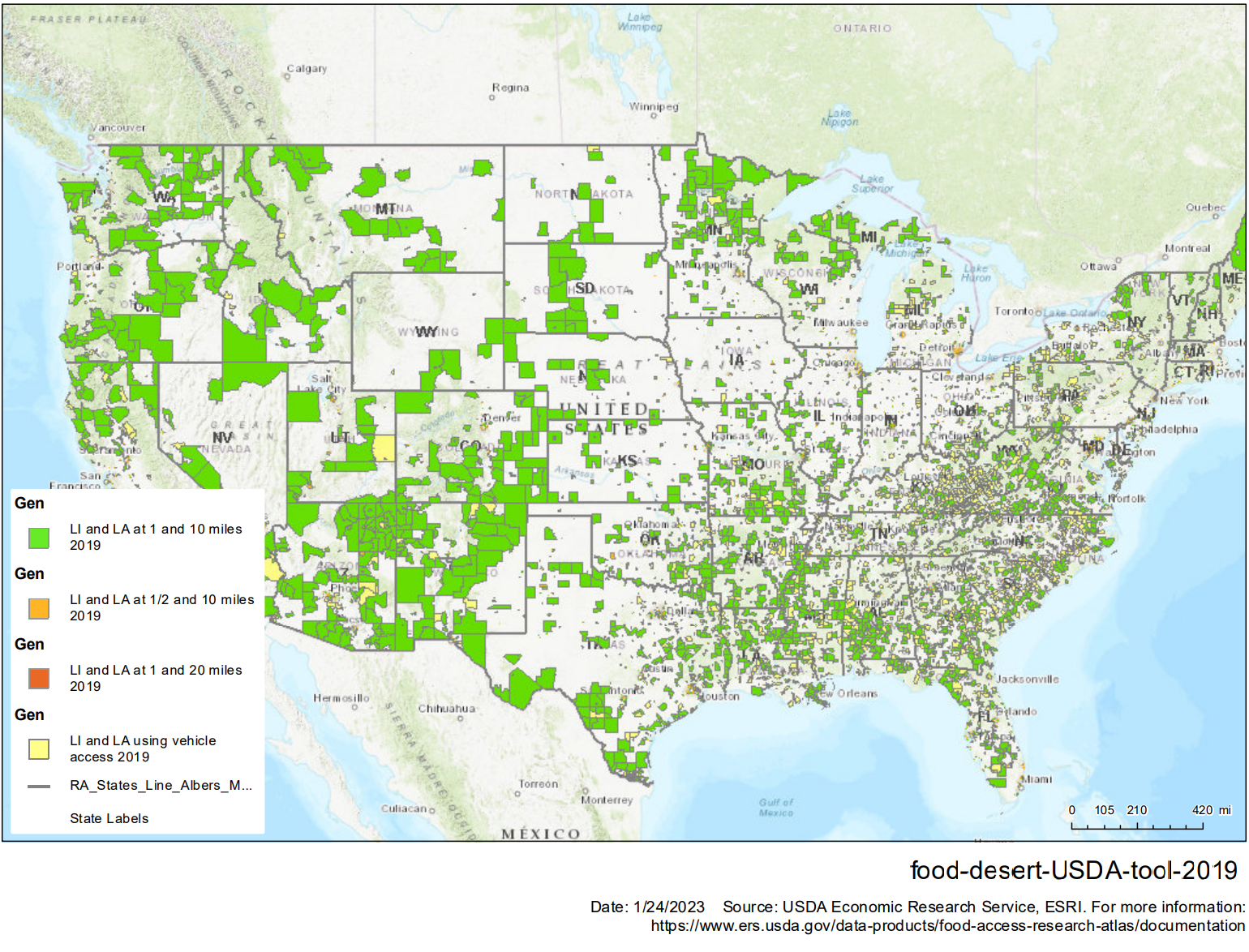
(a) Survey by USDA Economic Research Service shows that a large fraction of the American population is poor and without access to a grocery store with fresh food within 1-10 miles.

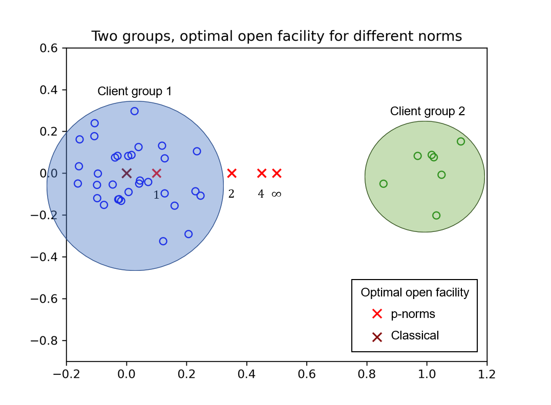
(b) A simulated example for fair facility location. We have two groups of clients. Optimal open facility for different norms are shown as red crosses. The $1$-norm optimal facility is close to the center of the larger group, while the $\infty$-norm facility is equidistant from the two groups.

Figure 1:

Example. Consider Figure 1(b) with clients $D$ partitioned into two groups (marked in blue and green), centered around the points $(0,0)$ and $(1,0)$ respectively. A facility can be opened anywhere on line segment joining the two points, and facility cost increases linearly from left to right. The classical optimal solution opens a facility close to $(0,0)$ since the first client group has a larger population and facility cost is lower. However, if we minimize the maximum average distance along with facility cost instead, we get an open facility equidistant from the two groups.

Assuming that the distances model an “access” cost, one can then ask if there is a way to open facilities so that different groups of people have an equitable access to these facilities. Let the groups partition the demand/clients into disjoint subsets (e.g., groups could be based on insurance status, income levels, race, age groups, etc). We consider in this work an equity-inducing term in the objective that minimizes the $L_{p}$ norm of the average group distances to the assigned facilities, along with the cost of opening these facilities. Formally, we define the following:

Definition (Fair facility location).

Suppose we are given a metric space $\mathcal{M}=(X,d)$, client set $D\subseteq X$, a non-empty set of facilities $F\subseteq X$ with non-negative facility costs $c:F\to\mathbb{R}_{+}$, and non-empty and disjoint client groups $D_{1},\ldots,D_{r}$ that partition $D$. For $p\in[1,\infty]$, the $p$-norm fair facility location problem requires opening a subset of facilities $F^{\prime}\subseteq F$ with a client to facility assignment $\Pi:D\to F$ to minimize the cost of open facilities and the Minkowski $p$-norm of average group distances $d(D_{s})=\frac{1}{|D_{s}|}\sum_{j\in D_{s}}d(j,\Pi_{j})$, i.e.,

$$\min\underbrace{\sum_{i\in F^{\prime}}c_{i}}_{\text{Facility cost }C_{F^{\prime}}}+\underbrace{\big{\|}\big{(}d(D_{1}),\ldots,d(D_{r})\big{)}\big{\|}_{p}}_{\text{Assignment cost }C_{\Pi}}.$$

For $p=1$ and singleton groups (i.e., $|D_{s}|=1$ for all $s\in[r]$), this reduces to the aforementioned classic facility location problem. For $p=\infty$, the objective corresponds to minimizing the maximum distance across all groups, weighted by their group size. This variant has been studied generally [9, 39] and in specific contexts (for example, emergency rooms placement [14]). A solution $\mathcal{S}=(F^{\prime},\Pi)$ to an instance is an ordered pair of open facilities and an assignment function which maps clients to open facilities (e.g., not necessarily to the closest facilities), with the cost of $\mathcal{S}$ denoted $C_{\mathcal{S}}=C_{F^{\prime}}\text{ (facility cost)}+C_{\Pi}\text{ (assignment cost)}$. Note that although we have defined our objective for average distance to open facilities for each group, our results hold for a larger class of objectives, including total distance to open facilities for each group.

Choice of $p$. In the above formulation, the choice of $p$ might lead to widely varying set of opening facilities, that induce different group access costs. For example, in Figure 1(b), note the optimal solutions for $p\in\{1,2,4,\infty\}$ are spread out on the real line. What is then unclear is that which choice of $p$ makes up the “fairest” equity objective? The chosen $p$ allows the optimization to weigh the connection cost paid by different socioeconomic groups differently, and what this weighting should be may not be clear even to the algorithm designer. Therefore, instead of selecting a specific $p$, we will attempt to construct a small set of solutions to the facility location problem, so that at least one of these solutions is “approximately” close to the best solution under any fixed $p$. It is a priori unclear why such a small set of solutions should even exist. Indeed, for classification algorithms, it has been shown that different fairness objectives may not be simultaneously satisfied (even approximately) [31, 12].

To explore this, we first consider the natural question: is an optimal solution to the $p$-norm fair facility problem a “good” approximation to the $q$-norm fair facility problem for different $p,q\in[1,\infty]$? This is not always the case; indeed, the cost of an optimal solution to the $p$-norm problem can be high ($\Omega(r)$, where $r$ is the number of client groups) for the $q$-norm problem. This raises the following question: is there a small set of candidate solutions such that no matter what norm is chosen, one of the solutions in the set is a “good” approximation corresponding to that norm? Empirical studies suggest that this might possibly be true even for an infinite class of objective functions (e.g., [25] show data-dependent constant-factor approximations for an infinite set of objectives that trade-off efficiency and a fixed equity term). As one of our first main results, we answer this question positively.

• Result 1. (Theorem 2, Section 2) There exist $\sim\log_{2}r$ solutions such that for each $p\in[1,\infty]$, one of these solutions is an $8$-approximation for the $p$-norm fair problem, where $r$ is the number of groups.

The above result provides an interesting way to get around the choice of $p$. Such portfolio design problems for multi-criteria approximation have not received enough attention from the theory community. Once a good portfolio is constructed, the most appropriate notion of ‘fairness’ matters less. A decision maker can simply weigh the properties of the solutions in the portfolio (potentially including external factors as well), and make an informed choice. This practice is common in other critical resource allocation scenarios, such as for organ transplants. United Network for Organ Sharing (UNOS) chooses a policy for kidney transplants after carefully considering a portfolio of candidate policies and evaluating them on multiple axes of interest [1].

We next consider if $O(\log_{2}r)$ is the right bound in the first result on construction of good portfolios, or if there could exist a single solution to the facility location problem which well approximates all $p$-norms for $p\geq 1$ (i.e., a portfolio of size 1)? We show that these portfolio must at least be $\sqrt{\log r}$ in size, in the worst-case, and a dependence on $r$ is in fact necessary.

• Result 2. (Theorem 3) There exist problem instances where at least $\tilde{\Omega}(\sqrt{\log_{2}r})$ different solutions are needed such that one of them is an $O(1)$-approximation for any $p$-norm.

Finally, when constructing a small portfolio of solutions, in general, there may not be any structure or commonality across the solutions in the portfolio. For example, consider a small portfolio of solutions in Figure 2, where each solution opens a completely disjoint set of facilities. This makes it harder to adapt the solutions in case the notion of fairness changes over time, for example, if facilities open by one of the solutions also remained open in another approximate solution, this would make planning more flexible to the demands of people as the need arises. We therefore aim to understand how approximate solutions change as $p$ varies, and if common combinatorial structure can be preserved between these approximate solutions for various norms. This question may be of independent interest from a multi-criteria optimization perspective: what common structures do optimal (or approximate) solutions maintain for related objectives.

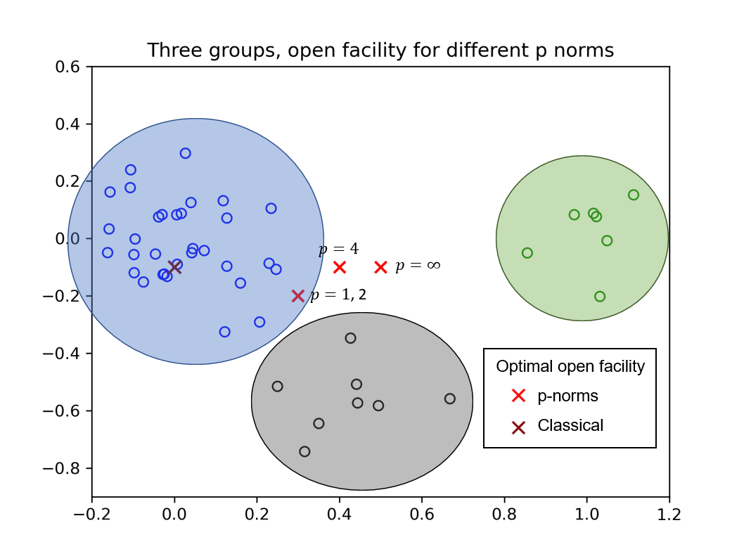
Figure 2: A simulated example for fair facility location with three groups. Facility cost increases linearly from left to right. Facilities opened in optimal solutions for fair facility location for different norms are shown as red crosses. The facility for $p=1$ is lower and to the left of the facility for $p=\infty$ since two close-by groups dominate the assignment cost for small $p$ and facility costs are smaller to the left. The classical optimal is far to the left.

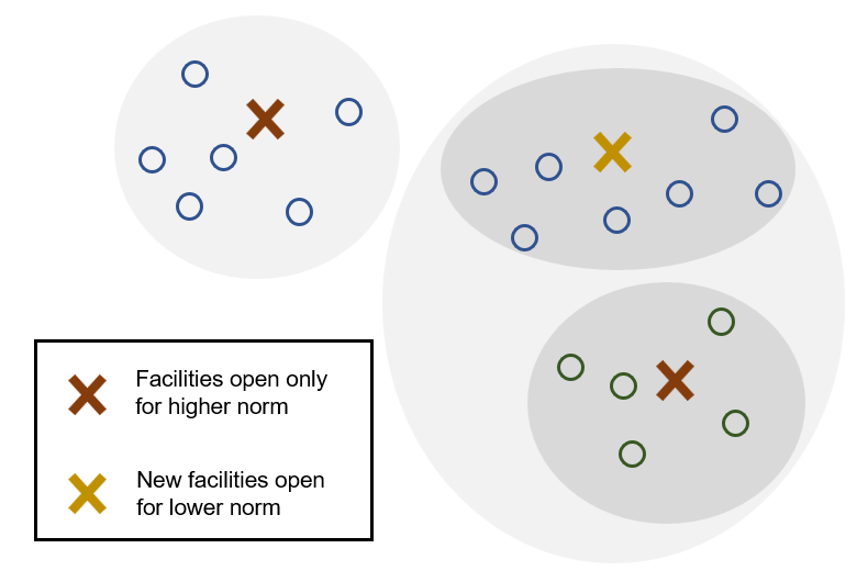
Figure 3: A toy example for refinement. The clients are drawn as circles and open facilities are drawn as crosses. As norm $p$ varies from $\infty$ to $1$ and the norm decreases, only new facilities are opened; no facilities open for higher norms are deleted. Additionally, when new facilities are opened, they can only serve a clients previously assigned to a single open facility.

We next study portfolio of solutions that satisfy a “refinement”-like structure. Consider two different solutions in our portfolio. We first ensure that the set of facilities open in one solution is a subset of the facilities open in the other. Moreover, we also demand the assignment of clients to facilities in the two solutions also satisfy additional properties. At a basic level, we ensure that if a facility that is open in the first solution is closed in the second solution, then the set of clients assigned to the closed facility are all reassigned to a single open facility in the second solution. In fact we ask for a stronger restriction when constructing portfolios: the assignment of the clients to open facilities induces a partition of clients. The partitions for two different solutions must be refinements of each other. This property can help maintain and plan capacity constraints when opening facilities like emergency rooms as well as make the choice of selecting the most suitable solution in the portfolio easier.

We next define “refinements” formally: for constraining the choice of open facilities, as well as where the clients must be served from.

Definition (Refinement).

We are given an instance of the fair facility location problem with non-empty client groups $D_{1},\ldots,D_{r}$ that partition $D$. Given a set of norms $P\subseteq[1,\infty]$, a solution set $S=\{\mathcal{S}_{p}=(F_{p},\Pi_{p}):p\in P\}$ is called a refinement if

1. (Facility condition) for all $p,q\in P$ with $p\leq q$, $F_{p}\supseteq F_{q}$; that is, the facilities form a decreasing subset structure with $p$, and

2. (Assignment condition) for all $p,q\in P$ with $p\leq q$ and for each facility $f\in F_{p}$, there is some facility $f^{\prime}\in F_{q}$ such that all clients assigned to $f$ under $\Pi_{p}$ are assigned to $f^{\prime}$ under $\Pi_{q}$, that is,

   $$\{j\in D:\Pi_{p}(j)=f\}\subseteq\{j\in D:\Pi_{q}(j)=f^{\prime}\}.$$

If for each norm $p\in P$, the solution $\mathcal{S}_{p}$ is an $\alpha$-approximation for the $p$-norm fair problem, then we say that the refinement is an $\alpha$-approximate refinement.

The second condition on assignments allows planning for capacity, and reallocations of clients to “parent” facilities, in case some facilities need to be closed. Constructing a portfolio of solutions that respects refinements is not only interesting from a planning perspective, but is also a technically interesting problem. In particular, we modify the portfolios in the previous step non-trivially to show that we can even find small portfolio with this additional structure enforced.

• Result 3. We present a $\mathrm{poly}(r^{\frac{1}{\sqrt{\log r}}})$-approximation for refinement for the norm set $P=[1,\infty]$ on arbitrary metrics (Section 3), and improve this to $O(\log r)$ for the special case of line metric (Appendix C.1).

At a high level, we use the set of $\sim\log r$ solutions from Result 1 as a proxy for the norm set $[1,\infty]$, and then change our assignments in these solutions recursively so that they satisfy the assignment condition for refinement while ensuring that no client is assigned to a far-away facility. Our techniques are not restricted to $p$-norm problems and work on more general settings, we apply then to a hierarchical version of the facility location problem as an example; see Section 5 and Appendix D.

1.1 Overview of techniques

Portfolio of soutions

Any candidate solution to a given instance of a problem incurs different costs for different $p$-norms. The ratio of the costs of a candidate solution for two different norms is bounded above by a fundamental relationship between different $p$-norms. For different norms $p,q$, This implies that the a constant-factor approximation solution for the $p$-norm fair problem is a constant-factor approximation for the $q$-norm fair problem as well, so long as $p$ and $q$ are close enough, specifically when $\left|\frac{1}{p}-\frac{1}{q}\right|=O\left(\frac{1}{\log r}\right)$. This locality of costs allows us to obtain about $\log_{2}r$ norms that can represent all norms in $[1,\infty]$. This representative set of norms will be further useful for refinement. Our proof uses ideas similar to those in [23].

Refinement

An $O(\log r)$-approximate refinement satisfying only the facility condition (Condition 1) can be obtained using the aforementioned representative set. Extending this to the assignment condition (2) is more challenging. The first idea is to reduce the problem for a infinite set of norms $P=[1,\infty]$ to a norm set of cardinality $\log_{2}r$, using the aforementioned representative set of norms. That is, we can restrict ourselves to getting refinement for a finite norm set $\{p_{1},\ldots,p_{l}\}$ with $l\simeq\log_{2}r$.

We present a natural greedy idea first that gives $2^{l}$-approximate (i.e an $r$-approximate) refinement. It contains the seeds of our recursive algorithm with an improved approximation ratio $\mathrm{poly}(e^{\sqrt{l}})=\mathrm{poly}(r^{\frac{1}{\sqrt{\log r}}})$.

Consider Figure 4: we are given a norm set $P=\{p_{1},\ldots,p_{l}\}$ with $p_{1}\leq\ldots\leq p_{l}$, and assume that we already have an $O(l)$-approximate refinement $\mathcal{S}=\{(F_{i},\Pi_{i}):i\in[l]\}$ satisfying the facility condition, i.e., $F_{1}\supseteq F_{2}\supseteq\ldots\supseteq F_{l}$. To satisfy the assignment condition, we modify assignments $\Pi_{k},k\in[l]$. To start, assign each client $j\in D$ first to their closest facility in $F_{1}$, say $f_{1}$, i.e., $\Pi_{1}(j)={\arg\min}_{f\in F_{1}}d(j,f)=f_{1}$. Next, map facility $f_{1}\in F_{1}$ to its closest facility $f_{2}\in F_{2}$, and assign $\Pi_{2}(j)=f_{2}$. This ensures that each client mapped to $f_{1}$ under $\Pi_{1}$ is mapped to $f_{2}$ under $\Pi_{2}$, i.e.

$$\{j\in D:\Pi_{1}(j)=f_{1}\}\subseteq\{j\in D:\Pi_{2}(j)=f_{2}\}.$$

Do this iteratively for each client $j$ and each assignment $\Pi_{1},\ldots,\Pi_{l}$. The greedy rule ensures that assignments $\Pi_{1},\ldots,\Pi_{l}$ satisfy the assignment condition.

Figure 4 shows how this can lead to large assignment costs for the $p_{l}$-norm problem, i.e., for assignment $\Pi_{l}$: the solution $(F_{l},\Pi_{l})$ produced by the greedy algorithm is only guaranteed to be a $(2^{l}-1)$-approximation to the $p_{l}$-norm problem.

In the example shown, a better solution is to map client $j$ at location $0$ to the facility at $-(1+\epsilon)$ under each assignment $\Pi_{1},\ldots,\Pi_{l}$. Greedy algorithm misses this solution because it only looks at assignments one step ahead at a time. Our crucial insight is that for each client $j\in D$, one can look at closest facilities for all norms: $f_{s}={\arg\min}_{f\in F_{s}}d(j,f)$. Instead of assigning $\Pi_{1}(j)=f_{1}$, we first look at distances $d(j,f_{1}),\ldots,d(j,f_{l})$, fix a parameter $\gamma\geq 1$ and select

$$s^{*}={\arg\min}_{s\in[l]}\frac{d(j,f_{s})}{\gamma^{s}}.$$

Since $F_{1}\supseteq\ldots\supseteq F_{s^{*}}$, we assign $\Pi_{s}(j)=f_{s^{*}}$ for all $s\leq s^{*}$. By definition of $s^{*}$, we are guaranteed that $d(j,\Pi_{s}(j))\leq\gamma^{s-s^{*}}d(j,f_{s})\leq\gamma^{l-1}$ for all $s\leq s^{*}$. For small enough $\gamma$, this will ensure that $(F_{s},\Pi_{s})$ is a good approximation to the $p_{s}$-norm fair problem.

For $s>s^{*}$, we can assign $\Pi_{s}(j)$ recursively by treating $f_{s^{*}}$ as a client in the recursive instance. This ensures that assignments $\Pi_{1},\ldots,\Pi_{l}$ satisfy the assignment condition and therefore form a refinement, although it takes some work to show this.

Notice that this reduces to the greedy algorithm for $\gamma=1$ since $F_{1}\supseteq\ldots\supseteq F_{l}$ and therefore $d(j,f_{1})\leq\ldots\leq d(j,F_{l})$. In choosing $s^{*}$, we are discounting the larger distance $d(j,f_{s})$ by a factor $\gamma^{s}$ as compared to $d(j,f_{1})$. We call this algorithm DiscountedLookahead. It is formalized and presented in Section 3.

Figure 4: A toy example to illustrate that the greedy algorithm for refinement can reassign clients to far away facilities. The underlying metric is a line metric. Each client is denoted by a circle, and facilities in $F_{1},\ldots,F_{l}$ are denoted as a cross at their respective locations, with a copy of the line for each $k\in[l]$ for clarity. For $\epsilon>0$, the closest facility in $F_{1}$ to the client at $x=0$ is at $x=1$, and so the greedy algorithm assigns $\Pi_{1}(0)=1$. Further, the closest facility to $x=1$ in $F_{2}$ is at $x=3$, so that $\Pi_{2}(0)=3$. Continuing this way, $\Pi_{l}(0)=2^{l}-1$. However, the closest facility to $x=0$ in $G_{l}$ is at $-(1+\epsilon)$. For $\epsilon\simeq 0$, this reassignment increases the distance by a factor $\simeq 2^{l}-1$ for the client at $x=0$.

1.2 Literature review

The classic facility location problem has been extensively studied. An $O(\log n)$-approximation algorithm without the metric assumption was given by Hochbaum [27]. Shmoys et al. [42] gave a deterministic $4$-approximation algorithm, the first $O(1)$-approximation. They also give a randomized $3.16$-approximation algorithm. Since then, a steady stream of algorithms has led to frequent improvements in this approximation factor [32, 11, 13, 28, 36, 10]. The state-of-the-art is a $1.488$-approximation algorithm of Li [34]; while the problem is inapproximable to within a factor $1.463$ unless $P=NP$ [24, 44]. See the textbook [47] gives for an overview.

Several fairness objectives for the facility location problem have been studied [29, 18, 45]; for an extensive list see the survey articles [38, 6]. To the best of our knowledge, none of these fairness objectives have been studied from an approximation algorithm viewpoint for facility location. However, several approximation algorithms are known for the fair versions of the related clustering problem where a fixed number of facilities are allowed to open [29, 20, 3, 37, 21, 23, 22].

Minkowski $p$-norm objectives have been widely considered in combinatorial optimization literature as a model for fairness and as interesting theoretical questions. Golovin et al. [23] develop a general technique for $p$-norm optimization that is closely related to our technique in section 2.1. Other methods are often problem-specific: for instance, $k$-clustering [20, 21, 22, 23], traveling salesman problem [17], set cover, scheduling and other problems [23] have all been studied with the $p$-norm objective.

There are a very large number of models for hierarchical facility location problems; see survey articles [49, 16]. Many of these models have not been studied from an approximation algorithm viewpoint. However, there are several models with an approximation guarantee for the overall cost [2, 8, 4, 5, 48, 30, 19, 46]. Almost all of these models aim to minimize some notion of the total cost or maximize some notion of client coverage that is linear in open facilities and assignments. To the best of our knowledge, a model to minimize the worst approximation ratio across different levels has not been proposed so far.

1.3 Preliminaries

We show that Shmoys et al.’s algorithm [42] – which uses the filtering technique introduced by Lin and Vitter [35] – extends to a much larger class of functions. For completeness, we include the algorithm and the proof of the theorem in Appendix A.

Before we state the theorem, we recall the definition of sublinear functions: $f$ is sublinear if for all $x,y$ in its domain (1) $f(cx)=cf(x)$ for all $c\geq 0$ and (2) $f(x+y)\leq f(x)+f(y)$. All norms are sublinear and all sublinear functions are convex.

Theorem 1.

Suppose we are given an instance of the facility location problem and function $f:\mathbb{R}_{+}^{D}\to\mathbb{R}_{+}$. For a solution $\mathcal{S}=(F^{\prime},\Pi)$ to the instance, consider the generalized objective

$$\sum_{i\in F^{\prime}}c_{i}+f\Bigg{(}\Big{(}d\big{(}j,\Pi(j)\big{)}\Big{)}_{j\in D}\Bigg{)},$$

where $\Big{(}d\big{(}j,\Pi(j)\big{)}\Big{)}_{j\in D}$ is the vector in $\mathbb{R}^{D}$ consisting of individual client distances.

If $f$ is a non-decreasing differentiable sublinear function, then there is $4$-approximation to the generalized facility location problem with a polynomial number of oracle calls to $f,\nabla f$.

The classic facility location corresponds to the case where $f(x)=\sum_{j}x_{j}$ for $x\in\mathbb{R}_{+}^{D}$, i.e., the total assignment cost is the sum of distances of individual clients. Since $p$-norm functions also satisfy the conditions of the theorem, we immediately have the following corollary:

Corollary 1.

There is a polynomial-time algorithm that gives a $4$-approximation for the $p$-norm fair facility location problem for any $p\in[1,\infty]$.

2 Portfolio of solutions

In this section, we give upper (Theorem 2) and lower (Theorem 3) bounds on the number of solutions such that given any $p$-norm, at least one of the solutions is an $O(1)$-approximation.

Definition (Approximate solution sets).

Given an instance of the fair facility location problem and some $\alpha\geq 1$, an $\alpha$-approximate solution set is a set $S$ of solutions such that for all norms $p\in[1,\infty]$, there is some solution in $S$ that is an $\alpha$-approximation to the $p$-norm fair facility location problem.

2.1 Upper bound

The key idea is to use the relationship between different $p$-norms in $\mathbb{R}^{r}$ that follows from Hölder’s inequality [43]:

Lemma 1.

For $p,q\in[1,\infty]$ with $p\leq q$ and any vector $x\in\mathbb{R}^{r}$, $\|x\|_{q}\leq\|x\|_{p}\leq r^{\frac{1}{p}-\frac{1}{q}}\|x\|_{q}$.

This allows us to prove the next lemma that states that approximate solutions for one norm can be translated into approximate solutions for a different norm, incurring an additional factor in the approximation ratio:

Lemma 2.

Given an instance of the fair facility location problem with $r$ groups and $1\leq p<q\leq\infty$, any $\alpha$-approximate solution to the $p$-norm fair problem is an $\big{(}\alpha r^{\frac{1}{p}-\frac{1}{q}}\big{)}$-approximate solution to the $q$-norm fair problem, and conversely, any $\alpha$-approximate solution to the $q$-norm fair problem is an $\big{(}\alpha r^{\frac{1}{p}-\frac{1}{q}}\big{)}$-approximate solution to the $p$-norm fair problem.

Recall that $OPT_{p}$ is a decreasing function of $p$. Define sequence $q_{1},\ldots,q_{T}$ as follows: $q_{1}=1$, $q_{k}$ is the unique norm satisfying $\frac{OPT_{q_{0}}}{OPT_{q_{k}}}=2^{k-1}$, and $T=\Big{\lceil}\log_{2}\left(\frac{OPT_{1}}{OPT_{\infty}}\right)\Big{\rceil}$. Also define $q_{T+1}=\infty$. From Lemma 1, we get that $OPT_{\infty}\leq rOPT_{1}$, so that $T\leq\lceil\log_{2}r\rceil$. This leads to the main result of this section:

Theorem 2.

Given any instance of the fair facility location problem, there exists an $8$-approximate solution set of cardinality at most $\lceil\log_{2}r\rceil$. This solution set can be obtained in polynomial time.

Proof.

Notice that

$$\frac{OPT_{q_{T}}}{OPT_{q_{T+1}}}=\frac{OPT_{1}}{2^{T-1}OPT_{\infty}}\leq\frac{2}{\frac{OPT_{1}}{OPT_{\infty}}}\cdot\frac{OPT_{1}}{OPT_{\infty}}=2.$$

Corollary 1 allows us to obtain $4$-approximate solutions for any $p$-norm for the given instance of the problem. We will claim that a $4$-approximate solution $\mathcal{S}_{k}=(F_{k},\theta_{k})$ to the $q_{k}$-norm fair problem is an $8$-approximate solution to the $p$-norm problem for any $p\in[q_{k},q_{k+1}]$. Since $\cup_{k=1}^{T}[q_{k},q_{k+1}]=[1,\infty]$, this implies that $\{\mathcal{S}_{1},\ldots,\mathcal{S}_{T}\}$ is an $8$-approximate solution set for the given instance of the facility location problem. Since $\left|\{\mathcal{S}_{1},\ldots,\mathcal{S}_{T}\}\right|=T\leq\lceil\log_{2}r\rceil$, this implies the theorem.

We prove the claim now. Let $V_{\theta_{k}}\in\mathbb{R}^{r}$ denote the cost vector for assignment $\theta_{k}$. Then, the cost of solution $\mathcal{S}_{k}$ for a norm $p\in[q_{k},q_{k+1}]$ is

$$C_{F_{k}}+\|V_{\theta_{k}}\|_{p}\leq C_{F_{k}}+\|V_{\theta_{k}}\|_{q_{k}}\leq 4OPT_{q_{k}}\leq 8OPT_{p}.$$

The first inequality follows from Lemma 1, the second inequality follows since $\mathcal{S}_{k}$ is a $4$-approximate solution to the $q_{k}$-norm fair problem, and the final inequality follows since $OPT_{q_{k}}\geq OPT_{p}\geq OPT_{q_{k+1}}\geq\frac{1}{2}OPT_{q_{k}}$. This proves the claim. ∎

Definition.

Given an instance of the facility location problem, we will call this set of norms $\{q_{1},\ldots,q_{T}\}$ the representative norm set. Getting $\alpha$-approximate solutions corresponding to these norms is sufficient to get $2\alpha$-approximate solutions for each norm in $[1,\infty]$.

2.2 Lower bound

Theorem 3.

For all large enough $r$, there is an instance of the fair facility location problem with $r$ clients such that at any $O(1)$-approximate solution set contains at least $\tilde{\Omega}\left(\log_{2}r\right)$ distinct solutions.

Proof.

We consider $r$ clients located at the central vertex of a star. We let $r=t^{k}$, where $t$ and $k$ are parameters that we will choose later; also let $\epsilon=\frac{1}{k}$. The star has $k$ edges with leaves $f_{1},\ldots,f_{k}$, leaf $f_{j}$ has facility with opening cost $t^{j}$ and is at distance $t^{(k-j)\epsilon}$ from the central vertex, for each $j\in[k]$. Each client is in its own group. This is presented in Figure 5.

For $i\in[k]$, let $p_{i}=\frac{k}{i}$. For appropriate choices of $t,k$, we will show that for distinct $i,i^{\prime}$, no $O(1)$-approximate solution to the $p_{i}$-norm fair problem is an $O(1)$-approximate solution to the $p_{i^{\prime}}$-norm fair problem. Therefore, any $O(1)$-approximate solution set for this problem instance contains at least $k$ distinct solutions.

Figure 5: The star graph instance in Theorem 3. There are $r=t^{k}$ clients at the central vertex and no clients at any of the leaf vertices. Leaf vertex $f_{i}$ has facility with cost $t^{i}$ and is at a distance $t^{(k-i)\epsilon}$ from the central vertex. The distances are marked in blue.

Fix $i\in[k]$. We show that any $O(1)$-approximate solution to the $p_{i}$-norm fair problem must have (a) the facility at $f_{i}$ open and (b) none of the facilities at $f_{i+1},\ldots,f_{k}$ open. This is sufficient to prove our claim.

If only $f_{i}$ is open, the solution cost for $p_{i}$-norm is

$$C_{p_{i},f_{i}} =t^{i}+\|t^{(k-i)\epsilon}\mathbf{1}_{r}\|_{p_{i}}=t^{i}+r^{\frac{1}{p_{i}}}t^{(k-i)\epsilon}=t^{i}+t^{i+(k-i)\epsilon}=\Theta(t^{i+(k-i)\epsilon}).$$

Since $\epsilon=\frac{1}{k}$, this cost is of the order $\Theta(t^{i+\frac{k-1}{k}})=\Theta(t^{(i+1)-\frac{1}{k}})$.

For a solution $\mathcal{S}$ with any of the facilities $f_{i+1},\ldots,f_{k}$ open, the solution cost $C_{\mathcal{S}}=\Omega(t^{i+1})$, which is higher than $C_{p_{i},f_{i}}$ by a factor $\Omega(t^{\frac{1}{k}})$. For $k=o(\log t)$, this factor is $\omega(1)$, and therefore $\mathcal{S}$ is not an $O(1)$-approximate solution to the $p_{i}$-norm fair problem.

Further, consider a solution $\mathcal{S}$ with none of the facilities $f_{i},\ldots,f_{k}$ open. At least one of the facilities in $f_{1},\ldots,f_{i-1}$ must be open, and even if all clients are assigned to the nearest open facility, the distance of each client from the nearest open facility is at least $t^{(k-(i-1))\epsilon}$. Therefore, the solution cost

$$C_{\mathcal{S}}=\Omega\left(\|t^{(k-i+1)\epsilon}\mathbf{1}_{r}\|_{p_{i}}\right)=\Omega\left(\|t^{(k-i+1)\epsilon}\mathbf{1}_{r}\|_{p_{i}}\right)=\Omega\left(t^{i+(k-i+1)\epsilon}\right).$$

This is higher than the cost of only opening $f_{i}$, i.e., $C_{p_{i},f_{i}}$ by a factor of $\Omega\left(t^{\frac{1}{k}}\right)$. For $k=o(\log t)$, this factor is $\omega(1)$, and therefore $\mathcal{S}$ is not an $O(1)$-approximate solution to the $p_{i}$-norm fair problem.

Finally, we show that for $k=\sqrt{\frac{\log_{2}r}{\log_{2}\log_{2}r}}$ and $k^{t}=r$, we have $k=o(\log t)$, finishing the proof. $t^{k}=r$ gives $\sqrt{\frac{\log_{2}r}{\log_{2}\log_{2}r}}\log_{2}t=\log_{2}r$ so that $\log_{2}t=\sqrt{\log_{2}r\cdot\log_{2}\log_{2}r}$, so that $k=o(\log_{2}t)$. ∎

3 Refinement

We discuss refinement in this section. One key idea is to use the local relationship between approximate solutions, i.e., use the representative norm set defined in 2.1. This allows us to focus only on finite norm sets, even when the we are required to produce refinement the entire norm set $P=[1,\infty]$. Therefore, we prove the following theorem for a finite norm set $P=\{p_{1},\ldots,p_{l}\}$, and obtain the result for $[1,\infty]$ as a Corollary:

Theorem 4.

Given a finite $P=\{p_{1},\ldots,p_{l}\}$ of norms, there is a polynomial-time algorithm that gives an $O(e^{3\sqrt{l}})$-approximate refinement for $P$.

Corollary 2.

There is a polynomial-time algorithm that gives a $\mathrm{poly}(r^{\frac{1}{\sqrt{\log_{2}r}}})$-approximate refinement for $P=[1,\infty]$ for arbitrary metrics.

Note that $e^{3\sqrt{l}}$ is subexponential in $l$ and $r^{\frac{1}{\sqrt{\log_{2}r}}}$ is sublinear in $r$: in fact, $r^{\frac{1}{\sqrt{\log_{2}r}}}=2^{\sqrt{\log_{2}r}}=o(r^{\delta})$ for all $\delta>0$. These peculiar functions arise as bounds on the terms of a recurrence relation that occurs naturally in our problem (see Lemmas 4, 5).

We improve the approximation ratio for the special case of line metric in Appendix C.1. From here on, we are primarily concerned by the order of our approximation ratios in terms of $r$. For convenience, we abuse the notation slightly and assume $\log_{2}r\simeq\lceil\log_{2}r\rceil$.

Suppose we are given a norm set $P=\{p_{1},\ldots,p_{l}\}$ with $p_{1}\leq\ldots\leq p_{l}$. As a first step, we show how to get a solution family $\mathcal{S}=\{(G_{k},\Pi_{k}):k\in[l]\}$ such that $(G_{k},\Pi_{k})$ is an $O(l)$-approximate solution to the $p_{k}$-norm fair problem and facility sets $G_{k},k\in[l]$ satisfy the facility condition, i.e., $G_{1}\supseteq\ldots\supseteq G_{l}$.

Here’s the idea: first obtain $4$-approximate solutions $(F_{k},\theta_{k})$ to the $p_{k}$-norm fair problems, $k\in[l]$. Define $G_{k}=F_{k}\cup F_{k+1}\cup\ldots\cup F_{l}$ for each $[k]$. Since $OPT_{p_{1}}\geq\ldots\geq OPT_{p_{l}}$, we have the following bound on the cost of $G_{k}$:

$$C_{G_{k}}=\sum_{t\geq k}C_{F_{t}}\leq\sum_{t\geq k}4OPT_{p_{t}}\leq 4lOPT_{p_{k}}.$$

3.1 Algorithm idea

Solutions $(G_{k},\theta_{k}),k\in[l]$ may still not satisfy the assignment condition. A natural approach is to reassign clients to facilities in each solution (i.e., for each $k\in[l]$) to satisfy the assignment condition. Such a reassignment may increase the assignment cost for each $k\in[l]$. Notice that we do not add any facilities to $G_{k},k\in[l]$ in any such reassignment. The key idea for Theorem 4 is to give a reassignment such that the distance of each client from its assigned facility increases by at most a factor $\beta$, and this enables us to convert the bound of $\beta$ into an approximate factor for refinement. We will show that $\beta=O(e^{3\sqrt{l}})$ for our algorithm.

Going ahead, we denote $G_{0}=D\cup G_{1}\ldots G_{l}$, so that $G_{0}\supseteq G_{1}\supseteq\ldots\supseteq G_{l}$. We will give more general assignments $\Pi_{k}:G_{0}\to G_{k}$ for all $k\in[l]$, and ensure that $d(j,\Pi_{k}(j))\leq\exp{3\sqrt{l}}\min_{f\in G_{k}}d(j,f)$ for all $j\in G_{0}$ and $k\in[l]$, so that solution $(G_{k},\Pi_{k})$ is an $O(\exp(3\sqrt{l}))$-approximation to the $p_{k}$-norm fair problem.

Recall that the greedy algorithm only has a guarantee of factor $2^{l}$ for the approximation ratio. One can think of the greedy algorithm as looking ‘one step’ ahead: for each $k\in[0,l-1]$ and each $f\in G_{k}$, map $\sigma(f)={\arg\min}_{h\in G_{k+1}}d(f,h)$. Then, for each client $j\in G_{0}$, the greedy algorithm assigns $\Pi_{k}(j)=\sigma^{k}(j)$. A natural question we consider here is if we can improve this algorithm by looking more than one step ahead at a time? Specifically, for client $j\in G_{0}$, instead of looking only at facility $f_{1}={\arg\min}_{f\in G_{1}}d(j,f)$, we can also look at facilities $h_{k}={\arg\min}_{h\in G_{k}}d(j,h)$ for $k\in[l]$ (that is, $h_{k}$ is the facility closest to $j$ in $G_{k}$, so that $f_{1}=h_{1}$). We pick some ‘discounting factor’ $\gamma>1$ to be chosen later, and instead of assigning $\Pi_{1}(j)=h_{1}$, we assign $\Pi_{s^{*}}(j)=h_{s_{*}}$ where

$$s_{*}={\arg\min}_{k\in[l]}\frac{d(j,h_{k})}{\gamma^{k}}.$$

Since $G_{k}\supseteq G_{s^{*}}$ for all $k\leq s^{*}$, we can assign $\Pi_{k}(j)=h_{s^{*}}$, and for $k>s^{*}$, we can do this process recursively for $G_{s^{*}},G_{s^{*}+1},\ldots,G_{l}$. Algorithm 1 does precisely this, and we show that this leads to a subexponential approximation factor in $l$.

For each $k\in[0,l-1]$ and each $t\in[k+1,l]$, the algorithm constructs an assignment $\Pi^{(k)}_{t}:G_{k}\to G_{t}$ from facilities at a lower level $k$ to facilities at a higher level $t$. The final assignments on clients $G_{0}=D$ are $\Pi_{k}^{(0)}:G_{0}\to G_{k}$ for $k\in[l]$.

3.2 Analysis

We need to prove two things about assignments $\Pi_{k}^{(0)},k\in[l]$: (1) they satisfy the assignment condition, and (2) $d(j,\Pi_{k}^{(0)})\leq\exp(3\sqrt{l})\min_{f\in G_{k}}d(j,f)$ for all $j\in G_{0}$, implying the approximation guarantee. We prove the first claim in the next lemma:

Obtain solutions $\{\mathcal{S}_{k}=(F_{k},\Pi_{k}):k\in[l]\}$ such that $\mathcal{S}_{k}$ is a $4$-approximation to the $p_{k}$-norm fair facility location problem ;

Denote $G_{k}=\cup_{t\in[k,l]}F_{t}$ for $k\in[l]$ ;

For any $k,t\in[0,l]$ and any $f\in G_{k}$, denote $h_{t}(f)={\arg\min}_{h\in G_{t}}d(f,h)$ ;

for $k=l-1$ to $0$ do

        for each $f\in G_{k}$ do

              

$$s^{*}={\arg\min}_{t\in[k+1,l]}\frac{d\left(f,h_{t}(f)\right)}{\gamma^{t}},$$

where $s^{*}$ is the least such number in case of ties. Let $h$ be the corresponding facility, i.e., $h=h_{s^{*}}(f)$ ;

               Set

$$\Pi^{(k)}_{t}(f)=\begin{cases}h&\text{if}\>t\in[k+1,s^{*}];\\ \Pi^{(s^{*})}_{t}(h)&\text{if}\>t\in[s^{*}+1,l]\end{cases}$$

        end for

       

end for

Output solutions $(G_{1},\Pi_{1}^{(0)}),\ldots,(G_{l},\Pi_{l}^{(0)})$

Algorithm 1 DiscountedLookahead

Lemma 3.

The assignments $\Pi_{1}^{(0)},\ldots,\Pi_{l}^{(0)}$ output by Algorithm 1 satisfy the assignment condition.

Proof.

First, we use induction on $l-k$ to prove the following: if $f\in G_{t}$, then $\Pi_{s}^{(k)}(f)=f$ for all $k<s\leq t$. When $k=l-1$, this is trivially true since $d(f,f)=0$. When $k<l-1$, $s^{*}=s+1$ and $h_{k+1}(f)=f$ in step 1 since $d(f,f)=0$ and $f\in G_{k+1}$. By induction, $\Pi_{t}^{(k+1)}(f)=f$, and since by step 1, we have $\Pi_{t}^{(k)}(f)=\Pi_{t}^{(k+1)}(h_{k+1}(f))$, we get $\Pi_{t}^{(k)}(f)=f$.

For convenience, define $\Pi_{k}^{(k)}:G_{k}\to G_{k}$, where $\Pi_{k}^{(k)}(f)=f$ for all $f\in G_{k}$. We prove the following claim: for all $0\leq k<s\leq t\leq l$ and for all (open) facilities $f\in G_{k}$ for $k\geq 1$ (and clients in $G_{0}$ for $k=0$),

$$\Pi_{t}^{(k)}(f)=\Pi_{t}^{(s)}\left(\Pi_{s}^{(k)}\left(f\right)\right).$$

We prove this using induction on $l-k$. For $k=l-1$, $s=t=l$, and by definition $\Pi_{l}^{(l)}\left(\Pi_{l}^{(k)}\left(f\right)\right)=\Pi_{l}^{(k)}\left(f\right)$.

Suppose $l-k>1$, i.e., $k<l-1$. As in Algorithm 1, let $s^{*}={\arg\min}_{s^{\prime}\in[k+1,l]}\gamma^{-s^{\prime}}d(f,h_{s^{\prime}}(f))$ and denote $h=h_{s^{*}}(f)$ for brevity in the proof that follows.

Case I: $s\leq t\leq s^{*}$. In this case, by step 1, $\Pi_{t}^{(k)}(f)=\Pi_{s}^{(k)}(f)=h$. Since $h\in G_{t}$, by our earlier claim, $\Pi_{t}^{(s)}(h)=h$, proving the desired equality.

Case II: $s<s^{*}\leq t$. Since $h\in G_{s^{*}}$, by our earlier claim we have $\Pi_{s^{*}}^{(s)}(h)=h$. Since $l-s^{*}<l-k$, using the induction hypothesis

$$\Pi_{t}^{(s)}(h)=\Pi_{t}^{(s^{*})}\left(\Pi_{s^{*}}^{(s)}\left(h\right)\right)=\Pi_{t}^{(s^{*})}(h).$$

By step 1, $\Pi_{s}^{(k)}(f)=h$ while $\Pi_{t}^{(k)}(f)=\Pi_{t}^{(s^{*})}(h)$, so that

$$\Pi_{t}^{(s)}\left(\Pi_{s}^{(k)}\left(f\right)\right)=\Pi_{t}^{(s)}(h)=\Pi_{t}^{(s^{*})}(h)=\Pi_{t}^{(k)}(f).$$

Case III: $s^{*}\leq s\leq t$. Since $l-s<l-k$, by the induction hypothesis,

$$\Pi_{t}^{(s^{*})}(h)=\Pi_{t}^{(s)}\left(\Pi_{s}^{(s^{*})}\left(f\right)\right).$$ (1)

In this case, $\Pi_{t}^{(k)}(f)=\Pi_{t}^{(s^{*})}(h)$ and $\Pi_{s}^{(k)}(f)=\Pi_{s}^{(s^{*})}(h)$, thus proving the desired equality and consequently the claim.

Facility sets $G_{1}\supseteq\ldots\supseteq G_{l}$ already satisfy the facility condition. To prove that assignments $\Pi_{1}^{(0)},\ldots,\Pi_{l}^{(0)}$ satisfy the assignment condition, we need to show that for all $k\in[1,l-1]$ and for all $f\in G_{k}$, there exists some $f^{\prime}\in G_{k+1}$ such that each client assigned to $f$ under $\Pi_{k}^{(0)}$ is assigned to $f^{\prime}$ under $\Pi_{k+1}^{(0)}$, that is:

$$\left\{j\in G_{0}:\Pi_{k}^{(0)}(j)=f\right\}\subseteq\left\{j\in G_{0}:\Pi_{k+1}^{(0)}(j)=f^{\prime}\right\}.$$

We claim that $f^{\prime}=\Pi_{k+1}^{(k)}(f)$ works.

Suppose $j\in G_{0}$ is such that $\Pi_{k}^{(0)}(j)=f$. Then $j$ must have been assigned to $f$ under $\Pi_{k}^{(0)}$ in one of the two cases in step 1. Let $s^{*}$ be the corresponding index chosen when $j$ is assigned.

If $k<s^{*}$, then $f=\Pi_{k}(j)=\Pi_{k+1}(j)=h_{s^{*}}(j)$. Since $h_{s^{*}}(j)\in G_{k+1}$, $\Pi_{k+1}^{(k)}\big{(}h_{s^{*}}(j)\big{)}=h_{s^{*}}(j)$.

If $k\geq s^{*}$, then $f=\Pi_{k}^{(0)}(j)=\Pi^{(s^{*})}_{k}\big{(}h_{s^{*}}(j)\big{)}$ and $\Pi_{k+1}^{(0)}(j)=\Pi_{k+1}^{(s^{*})}\big{(}h_{s^{*}}(j)\big{)}$. By eqn. (1),

$$\Pi_{k+1}^{(0)}(j)=\Pi_{k+1}^{(s^{*})}\big{(}h_{s^{*}}(j)\big{)}=\Pi_{k+1}^{(k)}\Big{(}\Pi_{k}^{(s^{*})}\big{(}h_{s^{*}}(j)\big{)}\Big{)}=\Pi_{k+1}^{(k)}(f).$$

∎

Before we prove our main theorem for this section, we need the following technical lemmas; we include their proofs in Appendix C.

Lemma 4.

Given $\gamma>1$ and some $l\in\mathbb{Z}_{+}$, consider the set of recursively defined numbers $\{u_{k,t}:t\in[l],k\in[0,t-1]\}$: for each $t\in[l]$, and for $k=t-1,\ldots,0$ define

$$u_{k,t}=\begin{cases}\gamma^{l-t}&\text{if}\>k=t-1,\\ \max\big{\{}\gamma^{l-t},\max_{k<s<t}\gamma^{s-t}+u_{s,t}(1+\gamma^{s-t})\big{\}}&\text{if}\>k\in[0,t-2].\end{cases}$$ (2)

Then $\max_{k,t}u_{k,t}\leq e^{\frac{2\gamma}{\gamma-1}}\gamma^{l-1}$.

Lemma 5.

$\min_{\gamma>1}e^{\frac{2\gamma}{\gamma-1}}\gamma^{l-1}\leq e^{2}\cdot e^{3\sqrt{l}}$.

We are ready to prove the approximation guarantee for Algorithm 1, and therefore our theorem:

Proof of Theorem 4.

Lemma 3 shows that Algorithm 1 gives a refinement for $P$. It remains to determine the choice of the parameter $\gamma$ and prove the desired bound on the approximation ratio.

Assume without loss of generality that $p_{1}<\ldots<p_{l}$; we know that $OPT_{p_{1}}\geq\ldots\geq OPT_{p_{l}}$. In step 1 of the algorithm,

$$C_{G_{k}}\leq\sum_{t\in[k,l]}C_{F_{t}}\leq 4\sum_{t\in[k,l]}OPT_{p_{t}}\leq 4\sum_{t\in[k,l]}OPT_{p_{k}}\leq 4l\>OPT_{p_{k}}.$$

If $\theta_{k}:D\to G_{k}$ assigns every client to its closest vertex in $G_{k}$, we have $C_{\theta_{k}}\leq C_{\Pi_{k}}$ since $G_{k}\supseteq F_{k}$. We will show that assignments $\Pi_{k}^{(0)}$ output by the algorithm satisfy $C_{\Pi_{k}^{(0)}}\leq O(e^{3\sqrt{l}})C_{\theta_{k}}$, and therefore that

$$C_{(G_{k},\Pi_{k}^{(0)})}=C_{G_{k}}+C_{\Pi_{k}^{(0)}}\leq 4l\>OPT_{p_{k}}+O(e^{3\sqrt{l}})C_{\Pi_{k}}\leq\left(l+O(e^{3\sqrt{l}})\right)OPT_{p_{k}}=O(e^{3\sqrt{l}})\>OPT_{p_{k}}.$$

To this end, it is sufficient to show that the assignments $\Pi_{1}^{(0)},\ldots,\Pi_{1}^{(l)}$ satisfy

$$d\left(j,\Pi^{(0)}_{k}(j)\right)\leq O(e^{3\sqrt{l}})\>d(j,h_{k}(j)),\quad\forall\>j\in D.$$ (3)

Instead of proving (3), we prove the following stronger inductive statement:

$$d\left(f,\Pi^{(k)}_{t}(f)\right)\leq u_{k,t}\>d(f,h_{t}(f)),\quad\forall\>f\in G_{k},\>\forall\>k\in[0,l-1],t\in[k+1,l].$$ (4)

where $u$ is the sequence defined in Lemma 4. Lemmas 4, 5 then imply (3).

We induct on $l-k$. Base case: $l-k=1$. Consider any $f\in G_{k}$, and let $s^{*}$ be the index in $[k+1,l]$ chosen in step 1. As in the algorithm, we denote $h=h_{s^{*}}(f)$. Then $s^{*}=l$, $h=h_{l}(f)$, and $\Pi_{l}^{(k)}(f)=h_{l}(f)$, so that (4) is trivially true.

Suppose $l-k>1$. Consider any $f\in G_{k}$. We have two cases.

Case I: $t\leq s^{*}$. By definition, $\Pi_{t}^{(k)}(f)=h_{s^{*}}(f):=h$. By the choice of $s^{*}$, $\gamma^{-t}d(h_{t}(f),f)\geq\gamma^{-s^{*}}d(h,f)$, so that $d(h,f)\leq\gamma^{s^{*}-t}d(h_{t}(f),f)\leq\gamma^{l-t}d(h_{t}(f),f)\leq u_{k,t}d(h_{t}(f),f)$.

Case II: $t>s^{*}$. Since $s^{*}>k$, $l-s^{*}<l-k$, and so we have by the induction hypothesis that

$$d\left(h,\Pi^{(s^{*})}_{t}(h)\right)\leq u_{s^{*},t}\>d(h,h_{t}(h))\leq u_{s^{*},t}d(h,h_{t}(f)),$$

where the last inequality follows since by definition $h_{t}(h)$ is the closest facility to $h$ in $G_{t}$. Therefore, we have

$$d\left(f,\Pi^{(k)}_{t}(f)\right) \leq d(f,h)+d\left(h,\Pi^{(k)}_{t}(f)\right)=d(f,h)+d\left(h,\Pi^{(s^{*})}_{t}(h)\right)$$

$$\leq d(f,h)+u_{s^{*},t}\cdot d\left(h,h_{t}(f)\right)\leq d(f,h)+u_{s^{*},t}\cdot\big{(}d(f,h)+d\left(f,h_{t}(f)\right)\big{)}.$$

The first and final inequalities are triangle inequalities. The equality is by definition of $\Pi^{(k)}_{t}(f)$ and $s^{*}$.

Now, since $s^{*}={\arg\min}_{t\in[k+1,l]}d(f,h_{t}(f))$, we have $d(f,h)\leq\gamma^{s^{*}-t}d(f,h_{t}(f))$, so that the above inequality becomes

$$d\left(f,\Pi^{(k)}_{t}(f)\right)\leq d\big{(}f,h_{t}(f)\big{)}\times\Big{(}\gamma^{s^{*}-t}+u_{s^{*},t}\cdot\big{(}\gamma^{s^{*}-t}+1\big{)}\Big{)}.$$

Since

$$u_{k,t}\geq\max_{k<s<t}\Big{(}\gamma^{s-t}+u_{s,t}\cdot\big{(}\gamma^{s-t}+1\big{)}\Big{)}\geq\gamma^{s^{*}-t}+u_{s^{*},t}\cdot\big{(}\gamma^{s^{*}-t}+1\big{)},$$

we get that $d\left(f,\Pi^{(k)}_{t}(f)\right)\leq d\big{(}f,h_{t}(f)\big{)}\times u_{k,t}$. ∎

4 Discussion

To demonstrate our model on real-world data, we compute a portfolio of good solutions in an empirical study on Census tracts in Fulton County, Georgia, USA. Each Census tract is a local group of a few thousand individuals located in the same geographic area, and Fulton County comprises of 199 Census tract. Each tract (weighted by its population) is treated as a client in our model. We categorize each Census tract in one of four socioeconomic groups, based on whether the population in the Census tract has is majority white and whether the median income in that tract is above a fixed income threshold (fixed to be USD $55000$ in this case). Opening a facility costs either $1,2$ or $4$ units, scaled roughly according to real-estate prices at the facility’s location. This model is general, and these facilities could correspond to hospitals, schools, corporate offices etc.

For a given $p\in[1,\infty]$ and a fixed $\lambda>0$, the objective is to minimize

$$\sum_{i:i\text{ is open}}c_{i}+\lambda\left\|(d_{A},d_{B},d_{C},d_{D})\right\|_{p},$$

where $d_{X}$ is the average (weighted by population) distance of Census tracts from their closest open facility in socioeconomic group $X$. That is, if census tract $j$ has population $n_{j}$ and is at distance $d_{j}$ from its nearest open facility, then

$$d_{X}=\frac{\sum_{j\in X}n_{j}d_{j}}{\sum_{j\in X}n_{j}},\quad X\in\{A,B,C,D\}.$$

$\lambda$ is a fixed constant to translate between distance units and facility cost units, chosen in our case to equal $100$. $\lambda$ can be varied to open a smaller or a larger number of facilities, depending on the application domain and trade-off between facility and assignment costs.

Figure 6 shows a two-solution portfolio for all norms. The first solution (with open facilities marked as squares) is a $2$-approximation for each $p$-norm fair problem, $p\in[1,2]$, and the second solution (with open facilities marked as circles) is a $2$-approximation for each $p$-norm fair problem, $p\in[2,\infty]$.

Table 1 gives the average distances $d_{X}$ for each socioeconomic group in each of the two solutions. Notice that each group has smaller average distance in the first solution, but this is traded-off by larger facility cost.

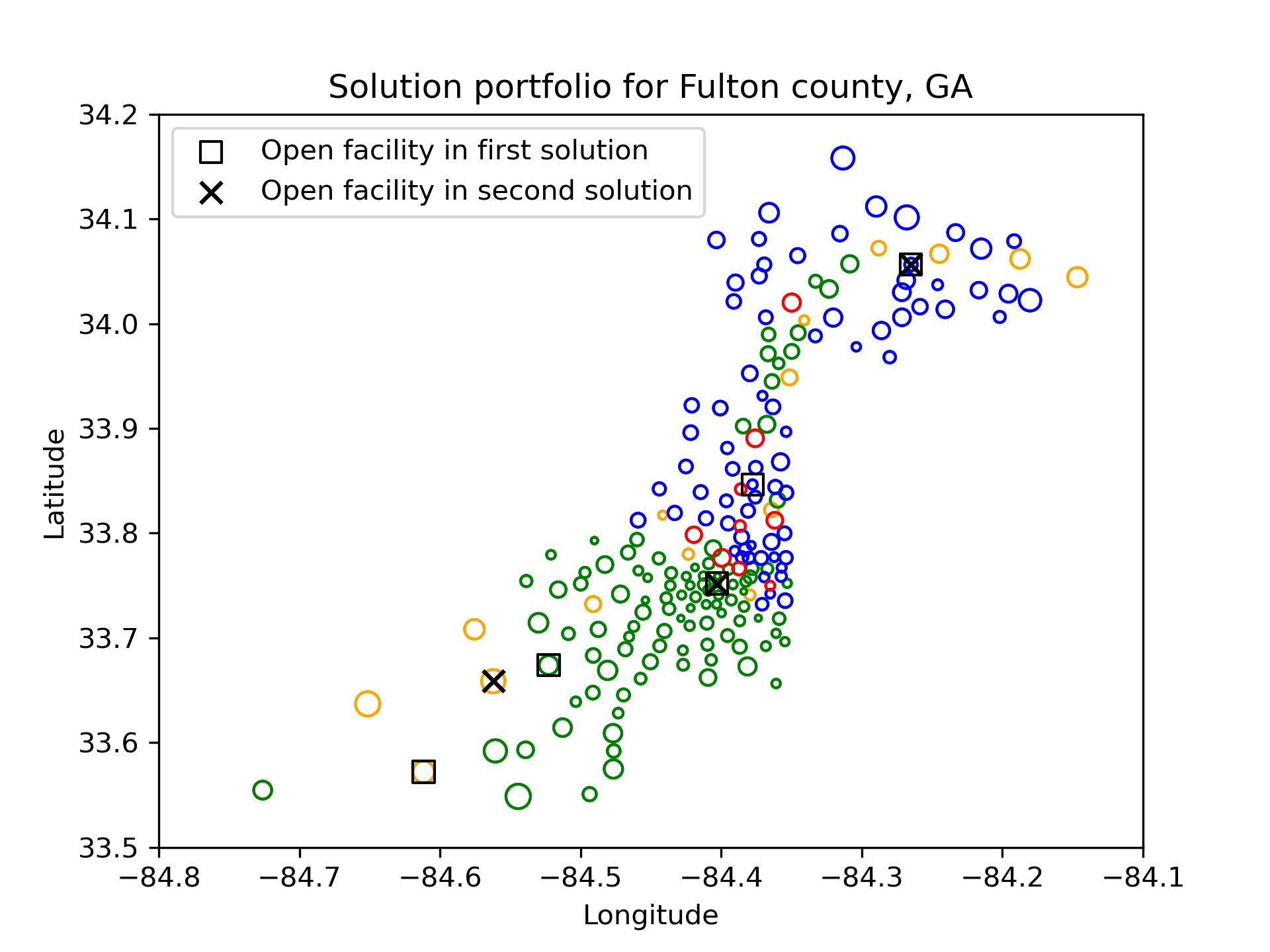
Figure 6: Census tracts and proposed solution portfolio for Fulton county, Georgia, USA. Each tract is represented by a circle with size proportional to its population, and tracts in different socioeconomic groups have different colors.

Socioeconomic groups	A	B	C	D	Number of open facilities
First solution	6.11	4.46	5.49	5.95	5
Second solution	8.13	7.26	6.62	7.51	3

Table 1: Average distances traveled (in km) by different socioeconomic groups in the two solutions in the portfolio. The four socioeconomic groups correspond to – $A$: above threshold income and majority white (in blue in the plot), $B$: below threshold income and majority white (in red), $C$: above threshold income and non-majority white (in orange), and $D$: below threshold income and non-majority white (in green).

5 Conclusion and Open questions

We studied a fair version of the classic facility location problem using Minkowski $p$-norms. We discussed portfolio of solutions that give approximate solutions for all norms, and then discussed refinement that imposes additional structure on this portfolio.

We talk about another application of our work next, and then discuss some open questions.

5.1 Other applications

Our techniques for refinement assume very little about the problem instances: in particular, for $p$-norms, we only use the fact that $OPT_{p}$ is decreasing in $p$ and $OPT_{1}/OPT_{\infty}\leq r$ for $r$ groups. As a result, our algorithms generalize to a much larger class of problems.

As an example, we introduce a version of the hierarchical facility location problem. In several applications of the facility location problem such as the placement of corporate offices, judicial courts, hospitals, and public works offices, facilities need to be opened at several hierarchical levels with additional constraints across those levels [16, 49]. For instance, public works offices usually operate at several levels, with the office at the lowest level serving as the first point of contact for an applicant (i.e., a client in facility location terms). The cost of opening a facility at a level increasing with the level. Usually, each open facility at a given level is also open at a lower level. Finally, for administrative purposes, all clients of a facility at a given level must be clients of the same facility at a higher level – this condition is often true for hierarchical structures.

As another motivation, consider schools: they are usually organized at a primary, middle, and high schools. High schools typically have a higher opening and maintenance cost than middle schools, which in turn have higher opening costs than elementary schools. Additionally, students studying the same primary school usually plan to attend the same middle school, and similarly with students attending the same high school.

For $l$ hierarchical levels, our version of the hierarchical facility location problem demands solutions for each of the $l$ levels of the given instance of the problem that satisfy the hierarchical constrains discussed above. We define it formally:

Definition (Hierarchical facility location).

We are given a metric space $\mathcal{M}=(X,d)$, and non-empty facility set $F\subseteq X$ and client/demand set $D\subseteq X$, and $l$ different classic facility location problems for some positive integer $l$, one for each level in $[l]$. The $l$ problems are specified by uniform facility opening costs $c_{1},\ldots,c_{l}\in\mathbb{R}_{+}$ satisfying $c_{1}\leq\ldots\leq c_{l}$. In the hierarchical facility location problem, we are asked to provide solutions $\{\mathcal{S}_{k}=(F_{k},\Pi_{k}):k\in[l]\}$ such that for all $k,t\in[l]$ with $t\geq k$:

1. $F_{k}\supseteq F_{t}$, and

2. for all facilities $f\in F_{k}$, there exists a facility $f^{\prime}\in F_{t}$ such that

   $$\{j\in D:\Pi_{p}(j)=f\}\subseteq\{j\in D:\Pi_{q}(j)=f^{\prime}\}.$$

The objective is to minimize the worst approximation ratio among $l$ levels, that is, $\displaystyle\max_{k\in[l]}C_{\mathcal{S}_{k}}/OPT_{k}$, where $OPT_{k}$ is the optimal solution value for the classic facility location problem with facility costs $c_{k}$. We call this an $l$-level hierarchical facility location problem.

Note that the constraints for hierarchical facility location are similar to refinements for fair facility location. This is why our algorithms work for both refinement and hierarchical facility location. We present approximation algorithms for this problem in Appendix D.

5.2 Open questions

A natural open question is about the existence of a solution set with cardinality lesser than $\lceil\log_{2}r\rceil$ (Theorem 2, Section 2) that is constant-factor approximate for $P=[1,\infty]$. In particular, given any instance of the fair facility location problem, what is the order of the smallest number of solutions required: is it $\Theta(\sqrt{\log_{2}r})$, or $\Theta(\log_{2}r)$, or something between the two?

Another open question is whether the subexponential factor $e^{3\sqrt{l}}$ for refinement in Theorem 4 (Section 3) can be reduced to a polynomial factor. We believe that this should be true (potentially by searching a larger local neighborhood instead of a one-step for the Greedy algorithm):

Conjecture 1.

Given a finite set $P=\{p_{1},\ldots,p_{l}\}$ of norms, there is a polynomial-time algorithm that gives a $\mathrm{poly}(l)$-approximation to the refinement problem for arbitrary metrics.

A harder problem is to resolve the approximation order completely: are there any non-trivial lower bounds for refinement? While it seems highly unlikely, it is not entirely clear whether a dependence on $r$ is necessary.

It is natural to ask if the algorithm for line metric generalizes to Cartesian spaces $\mathbb{R}^{d}$, $d>1$, after perhaps losing an additional factor that depends on $d$ ($2^{d}$, for instance).

Finally, it is natural to ask the basic question about the approximability of the $p$-norm fair facility location problem (see Theorem 1): can it be approximated to a factor better than $4$ in polynomial time? Several improved approximation factors are known for the classic facility location problem [47], including the $1.488$-approximation algorithm of Li. Most of these algorithms crucially use the linearity of the objective, and therefore do not generalize.

Appendix A Proof of Theorem 1

We can formulate the problem as an integer program: for each facility $i\in F$, variable $y_{i}\in\{0,1\}$ indicates whether facility $i$ is opened and for each client $j\in D$, variable $x_{ij}\in\{0,1\}$ indicates whether $j$ has been assigned to $i$. The feasible region is

$$\sum_{i\in F}x_{ij} \geq 1, \forall\>j\in D,$$

$$x_{ij} \leq y_{i}, \forall\>i\in F,j\in D,$$

$$x_{ij},y_{i} \in\{0,1\}, \forall\>i\in F,j\in D,$$

and the objective is to minimize the function $\sum_{i\in F}c_{i}y_{i}+f\left(\left(\sum_{i\in F}x_{ij}d(i,j)\right)_{j\in D}\right)$.

In the relaxation, we allow variables $x,y$ to take values in $[0,1]$:

$$\min_{x,y}\sum_{i\in F}c_{i}y_{i} +f\left(\left(\sum_{i\in F}x_{ij}d(i,j)\right)_{j\in D}\right)$$ subject to (CP)

$$\sum_{i\in F}x_{ij} \geq 1, \forall\>j\in D,$$ (5)

$$x_{ij} \leq y_{i}, \forall\>i\in F,j\in D,$$ (6)

$$0 \leq x,y.$$ (7)

Let us denote the underlying polytope by $P$ and the objective function by $\overline{f}:P\to\mathbb{R}$. Since $P$ has a polynomial number of constraints, the Ellipsoid algorithm (see [7]) can be used to obtain the following theorem:

Theorem 5.

For a differentiable convex function $f:\mathbb{R}^{D}\to\mathbb{R}$, an optimal solution to (CP) can be obtained in a polynomial number of calls to $f$ and $\nabla f$.

For the classical facility location problem with a linear objective, Shmoys et al. [42] use the filtering technique first introduced by Lin and Vitter [35] to round a fractional solution to (CP), giving a $4$-approximation. We show that their rounding algorithm generalizes to a much larger class of convex functions:

Lemma 6.

If $f$ is a sublinear function, then a fractional solution $(x,y)$ to (CP) can be rounded to an integral solution $(x^{*},y^{*})$ with cost $\overline{f}(x^{*},y^{*})\leq 4\overline{f}(x,y)$ in polynomial time.

This, along with Theorem 5 implies Theorem 1 for the general facility location problem and the corollary for $p$-norm socially fair facility location problem.

We present the algorithm now and then proceed to prove Lemma 6.

Set $\alpha=\frac{1}{4}$;

for $j\in D$ do

        Let $S_{j}=\{i\in F:x_{ij}>0\}$ ;

        Let $\sigma$ be the permutation arranging facilities in $S_{j}$ such that $d_{\sigma(1)j}\leq d_{\sigma(2)j}\leq\ldots$ ;

        Let $i_{j}={\arg\min}_{k}\sum_{k^{\prime}\in[k]}x_{\sigma(k^{\prime})j}\geq\alpha$, and let $d_{j}(\alpha)=d_{\sigma(i_{j}),j}$ ;

       

end for

for $i\in F$ do

        Set $\overline{y}_{i}\leftarrow\frac{1}{\alpha}y_{i}$ ;

        for $j\in D$ do

               Set $\overline{x}_{ij}$ to $\frac{1}{\alpha}x_{ij}$ if $d_{ij}\leq d_{j}(\alpha)$ and $0$ otherwise ;

              

        end for

       

end for

return $(\overline{x},\overline{y})$ ;

Algorithm 2 Filter$(x,y)$

Initialize $D^{\prime}\leftarrow D$ ;

Form a bipartite graph $G$ with vertex sets $D^{\prime},F^{\prime}$ with $ji\in E(G)$ iff $\overline{x}_{ij}>0$ for all $i\in F,j\in D$ ;

For $j\in D$, denote by $N_{G}(j)=\{i\in F:\overline{x}_{ij}>0\}$ the neighborhood of $j$ in $G$ and by $N^{2}_{G}(j)$ the set of all $j^{\prime}\in D$ that share a neighbor with $j$ in $G$, i.e., the set of all $j^{\prime}\in D$ with $N_{G}(j^{\prime})\cap N_{G}(j)\neq\emptyset$ ;

$k=0$ ;

while $D^{\prime}\neq\emptyset$  do

        Choose $j_{k}={\arg\min}_{j\in D^{\prime}}g_{j}$ ;

        Choose $i_{k}={\arg\min}_{i\in N_{G}(j_{k})}f_{i}$ ;

        Open $i_{k}$ and assign all $j\in N^{2}_{G}(j_{k})$ to $i_{k}$ ;

        $D^{\prime}\leftarrow D^{\prime}\setminus(N^{2}_{G}(j_{k})\cup\{j_{k}\})$, update $G$ ;

       

end while

Set $y^{*}_{i}=1$ for all opened facilities $i$, set $x^{*}_{ij}=1$ if $j$ was assigned to $i$, and set all other variables to $0$ ;

return $(x^{*},y^{*})$

Algorithm 3 Round$(\overline{x},\overline{y})$

Proof of Lemma 6.

Consider the solution $(\overline{x},\overline{y})$ output by Filter. Since $\overline{x}\leq\frac{1}{\alpha}x$ and $\overline{y}=\frac{1}{\alpha}y$, it satisfies the feasibility constraints (6) and (7). Further,

$$\sum_{i\in F}\overline{x}_{ij}=\sum_{i:d_{ij}\leq d_{j}(\alpha)}\frac{1}{\alpha}x_{ij}=\frac{1}{\alpha}\sum_{i:d_{ij}\leq d_{j}(\alpha)}x_{ij}\geq\frac{1}{\alpha}\times\alpha=1$$

by definition of $d_{j}(\alpha)$. Therefore, $\overline{x},\overline{y}$ is feasible.

Furthermore

$$\sum_{i\in F}d_{ij}x_{ij}\geq\sum_{i:d_{ij}\geq d_{j}(\alpha)}d_{ij}x_{ij}\geq d_{j}(\alpha)\sum_{i:d_{ij}\geq d_{j}(\alpha)}x_{ij}\geq d_{j}(\alpha)(1-\alpha).$$ (8)

Let the solution $(x^{*},y^{*})$ output by Algorithm Round. For the facility $i_{k}$ and client $j_{k}$ chosen in iteration $k$ of loop 3, by step 3 and since $\sum_{i\in F}\overline{x}_{ij_{k}}\geq 1$,

$$c_{i_{k}}\leq c_{i_{k}}\sum_{i\in F}\overline{x}_{ij_{k}}\leq\sum_{i\in N_{G}(j_{k})}c_{i}\overline{x}_{ij_{k}}\leq\sum_{i\in N_{G}(j_{k})}c_{i}\overline{y}_{i}.$$

Furthermore, since each client in set $N_{G}^{2}(j_{k})$ is assigned to $i_{k}$ and then removed from $G$, the client sets $N_{G}(j_{1}),N_{G}(j_{2}),\ldots$ are disjoint. Along with the above, this implies

$$\sum_{k}c_{i_{k}}\leq\sum_{k}\sum_{i\in N_{G}(j_{k})}c_{i}\overline{y}_{i}\leq\sum_{i\in F}c_{i}\overline{y}_{i}=\frac{1}{\alpha}\sum_{i\in F}c_{i}y_{i}.$$ (9)

Suppose client $j$ was assigned to $i_{k}$. Then $j\in N_{G}^{2}(j_{k})$ and by step 3, $d_{j}(\alpha)\geq d_{j_{k}}(\alpha)$. Since $j\in N_{G}^{2}(j_{k})$, there exists some $i\in N_{G}(j)\cap N_{G}(j_{k})$. By metric property of $d$, $d_{i_{k}j}\leq d_{i_{k}j_{k}}+d_{ij_{k}}+d_{ij}$. Further, by step 2 and since $\overline{x}_{ij},\overline{x}_{ij_{k}},\overline{x}_{i_{k}j_{k}}>0$, we must have $d_{ij}\leq d_{j}(\alpha)$, $d_{ij_{k}}\leq d_{j_{k}}(\alpha)$ and $d_{i_{k}j_{k}}\leq d_{j_{k}}(\alpha)$, so that

$$d_{i_{k}j}\leq 2d_{j_{k}}(\alpha)+d_{j}(\alpha)\leq 3d_{j}(\alpha).$$

Eqn. (8) then implies that $d_{i_{k}j}\leq 3d_{j}(\alpha)\leq\frac{3}{1-\alpha}\sum_{i\in F}x_{ij}d_{ij}$, or that $d_{i_{k}j}=\sum_{i\in F}x^{*}_{ij}d_{ij}\leq\frac{3}{1-\alpha}\sum_{i\in F}x_{ij}d_{ij}$. Since $f$ is nondecreasing and sublinear,

$$f\left(\left(\sum_{i}x^{*}_{ij}d_{ij}\right)_{j\in D}\right)\leq f\left(\left(\frac{3}{1-\alpha}\sum_{i}x_{ij}d_{ij}\right)_{j\in D}\right)=\frac{3}{1-\alpha}f\left(\left(\sum_{i}x_{ij}d_{ij}\right)_{j\in D}\right).$$

By eqn. (9),

$$\sum_{i\in F}c_{i}y_{i}^{*}=\sum_{k}c_{i_{k}}\leq\frac{1}{\alpha}\sum_{i\in F}c_{i}y_{i}.$$

Together, for $\alpha=\frac{1}{4}$, this implies that $\overline{f}(x^{*},y^{*})\leq 4f(x,y)$. ∎

Appendix B Missing proofs from Section 2

Proof of Lemma 2.

Let $OPT_{p},OPT_{q}$ denote the corresponding optimum values. Let $\mathcal{S}_{p}=(F_{p},\Pi_{p})$ be an $\alpha$-approximate solution to the $p$-norm fair problem, and let $C_{p}$ denote the assignment cost vector for it (so that the $p$-norm assignment cost of $\Pi_{p}$ is $\|C_{p}\|_{p}$). Let $\mathcal{S}_{q}^{*}=(F_{q}^{*},\Pi_{q}^{*})$ be an optimum solution to the $q$-norm fair problem, with assignment cost vector $C_{q}^{*}$.

We have from definition that $C_{F_{p}}+\|C_{p}\|_{p}\leq\alpha OPT_{p}$. Now,

$$C_{F_{p}}+\|C_{p}\|_{q} \leq C_{F_{p}}+\|C_{p}\|_{p}\leq\alpha OPT_{p}$$

$$\leq\alpha\big{(}C_{F_{q}^{*}}+\|C_{q}^{*}\|_{p}\big{)}\leq\alpha\big{(}C_{F_{q}^{*}}+r^{\frac{1}{p}-\frac{1}{q}}\|C_{q}^{*}\|_{q}\big{)}$$

$$\leq\alpha r^{\frac{1}{p}-\frac{1}{q}}\big{(}C_{F_{q}^{*}}+\|C_{q}^{*}\|_{q}\big{)}=\alpha r^{\frac{1}{p}-\frac{1}{q}}OPT_{q}.$$

where the first inequality follows from Lemma 1 and since $q>p$, the second inequality is true since $s_{p}$ is $\alpha$-approximate, the third inequality follows from definition, the fourth inequality follows from Lemma 1, the fifth inequality is true since $\frac{1}{p}-\frac{1}{q}>0$, and the final equality is true since $\mathcal{S}^{*}_{q}$ is an optimal solution to the $q$-norm fair problem. Therefore, $\mathcal{S}_{p}$ is a $\alpha r^{\frac{1}{p}-\frac{1}{q}}$-approximate solution to $q$-norm fair problem.

Similarly let $\mathcal{S}_{q}=(F_{q},\Pi_{q})$ be an $\alpha$-approximate solution to the $q$-norm fair problem with cost vector $C_{q}$. Then, using th fact that $OPT_{p}\geq OPT_{q}$,

$$C_{F_{q}}+\|C_{q}\|_{p} \leq C_{F_{q}}+r^{\frac{1}{p}-\frac{1}{q}}\|C_{q}\|_{q}\leq r^{\frac{1}{p}-\frac{1}{q}}\big{(}C_{F_{q}}+\|C_{q}\|_{q}\big{)}\leq\alpha r^{\frac{1}{p}-\frac{1}{q}}OPT_{q}\leq\alpha r^{\frac{1}{p}-\frac{1}{q}}OPT_{p}.$$

Therefore, $\mathcal{S}_{q}$ is an $\alpha r^{\frac{1}{p}-\frac{1}{q}}$-approximation to the $p$-norm fair problem ∎

Appendix C Missing proofs from Section 3

Proof of Lemma 4.

First, note that for any $t\in[1,l]$, since $\gamma>1$, we have

$$u_{t-1,t}\leq\ldots\leq u_{1,t}\leq u_{0,t},$$

so that it is enough to prove that $\max_{t}u_{0,t}\leq e^{\frac{2\gamma}{\gamma-1}}\gamma^{l-1}$. Further, since $u_{t-1,t}=\gamma^{l-t}$, this implies

$$u_{k,t}=\max_{k<s<t}\gamma^{s-t}+u_{s,t}(1+\gamma^{s-t})\quad\forall k\in[0,t-2].$$

First, a change of indices is in order: if we define $w_{k,t}=u_{t-1-k,t}$ for $k\in[0,t-1]$, we get $w_{0,t}=\gamma^{l-t}$ and

$$w_{k,t}=\max_{s\in[0,k-1]}\gamma^{-(s+1)}+w_{s,t}(1+\gamma^{-(s+1)})\quad\forall k\in[1,t-1].$$

This makes it clear that in fact

$$w_{k,t}=\gamma^{-k}+w_{k-1,t}(1+\gamma^{-k})\quad\forall k\in[1,t-1].$$

Finally, we bound $w_{t-1,t}=u_{0,t}$. Since $w_{0,t}=\gamma^{l-t}\geq 1$, notice that

$$\frac{w_{k,t}}{w_{k-1,t}}\leq\frac{\gamma^{-k}}{w_{k-1,t}}+1+\gamma^{-k}\leq 1+2\gamma^{-k}.$$

Therefore, taking product from $k=1$ to $t-1$, we get

$$\frac{w_{t-1,t}}{w_{0,t}}\leq\prod_{k=1}^{t-1}\left(1+2\gamma^{-k}\right).$$

Denote $P_{t}=\prod_{k=1}^{t-1}\left(1+2\gamma^{-k}\right)$. Using the standard bound $1+x\leq\exp(x)$,

$$\prod_{k=1}^{t-1}\left(1+2\gamma^{-k}\right)\leq\prod_{k=1}^{t-1}\exp\left(2\gamma^{-k}\right)=\exp\left(2\sum_{k=1}^{t-1}\gamma^{-k}\right)\leq\exp\left(2\sum_{k=1}^{\infty}\gamma^{-k}\right)=\exp\left(\frac{2\gamma}{\gamma-1}\right).$$

Therefore,

$$u_{0,t}=w_{t-1,t}\leq\exp\left(\frac{2\gamma}{\gamma-1}\right)w_{0,t}=\exp\left(\frac{2\gamma}{\gamma-1}\right)\gamma^{l-1}.$$

∎

Proof of Lemma 5.

Choose $\gamma=1+\frac{1}{\sqrt{l}}$. Then $e^{\frac{2\gamma}{\gamma-1}}=e^{2\sqrt{l}\left(1+\frac{1}{\sqrt{l}}\right)}=e^{2\sqrt{l}}\cdot e^{2}$. Also, $\gamma^{l-1}<\gamma^{l}=\left(1+\frac{1}{\sqrt{l}}\right)^{l}\leq\left(e^{\frac{1}{\sqrt{l}}}\right)^{l}=e^{\sqrt{l}}$, implying that $e^{\frac{2\gamma}{\gamma-1}}\gamma^{l-1}\leq e^{2}\cdot e^{3\sqrt{l}}$. ∎

C.1 Line metric

Consider the special case when the underlying metric $\mathcal{M}=(X,d)$ is a line metric, i.e., $X=\mathbb{R}$. We will denote by $x(f)\in\mathbb{R}$ the location of facility $f\in F$. In this section, we give an algorithm for an $O(\log_{2}r)$-approximate refinement for $P=[1,\infty]$. We prove the following theorem for a finite norm set, and obtain the result for $P=[1,\infty]$ as a corollary using the representative norm set defined in Section 2.

Theorem 6.

Given a finite set of norms $P$, there is a polynomial-time algorithm that gives an $O(|P|)$-approximate refinement for $P$ for the line metric.

Corollary 3.

There is a polynomial-time algorithm that gives an $O(\log_{2}r)$-approximate refinement for $P=[1,\infty]$ for the line metric.

We now develop the algorithm for $P=\{p_{1},\ldots,p_{l}\}$. Assume without loss of generality that $p_{1}<\ldots<p_{l}$, so that $OPT_{p_{1}}\geq\ldots\geq OPT_{p_{l}}$. Obtain a $4$-approximate solution $\mathcal{S}_{k}=(F_{k},\theta_{k})$ for each $k\in[l]$ using Corollary 1. The facility condition for refinement can be satisfied in a manner that we have deployed before: by combining facilities at all higher norms for each $p_{k}$. That is, define $G_{k}=\bigcup_{t\in[k,l]}F_{t}$. We can bound the facility costs $G_{k}$ for each $k$:

$$C_{G_{k}}\leq\Big{(}\sum_{t\geq k}C_{F_{t}}\Big{)}\leq\Big{(}\sum_{t\geq k}OPT_{p_{t}}\Big{)}\leq 4(l-(k-1))\>OPT_{p_{k}}\leq 4l\>OPT_{p_{k}}.$$ (10)

However, assignments $\theta_{k},k\in[l]$ may not satisfy the assignment condition. Suppose we construct assignments $\Pi_{k}:D\to G_{k}$, $k\in[l]$ so that

1. (Assignment condition) the solution set $T=\{(G_{k},\Pi_{k}):k\in[l]\}$ satisfy the assignment condition for $\{p_{1},\ldots,p_{l}\}$, and

2. (Cost upper bound) assignments $\Pi_{k}$ assign each client to a facility within a factor $1/\alpha$ of its nearest facility in $G_{k}$ for some fixed $\alpha\in(0,1]$. That is, for all $k\in[l]$,

   $$d\left(j,\Pi_{k}(j)\right)\leq\frac{1}{\alpha}\min_{f\in G_{k}}d\left(j,f\right)\quad\forall\>j\in D.$$ (11)

From the second condition, we have that $d\left(j,\Pi_{k}(j)\right)\leq\frac{1}{\alpha}\min_{f\in G_{k}}d\left(j,f\right)\leq\frac{1}{\alpha}d\left(j,\theta_{k}(j)\right)$ for all clients $j\in D$. From eqn. (10), we further have that $C_{G_{k}}\leq 4l\>OPT_{p_{k}}$. Therefore, since solution $\mathcal{S}_{k}=(F_{k},\theta_{k})$ is a $4$-approximate solution to the $p_{k}$-norm problem for each $k$, we can bound the cost of solution $(G_{k},\Pi_{k})$ for norm $p_{k}$:

$$C_{(G_{k},\Pi_{k})}=C_{G_{k}}+C_{\Pi_{k}}\leq 4l\>OPT_{p_{k}}+\frac{1}{\alpha}C_{\theta_{k}}\leq 4l\>OPT_{p_{k}}+\frac{4}{\alpha}\>OPT_{p_{k}}=\left(4l+\frac{4}{\alpha}\right)OPT_{p_{k}},$$

implying that if assignments $\Pi_{k},k\in[l]$ satisfy the two conditions above and if $1/\alpha=O(l)$, then the solution set $T=\{(G_{k},\Pi_{k}):k\in[l]\}$ forms an $O(l)$-approximate refinement for $\{p_{1},\ldots,p_{l}\}$.

Our algorithm achieves precisely these two conditions with $\alpha=\frac{1}{2l}$, implying Theorem 6. We first introduce some notation for this section. Then, we establish some structure on refinements on a line and give an outline of the algorithm.

Notation: We refer to $k\in\{1,\ldots,l\}$ as problem levels. Recall that $[l]$ indexes the set of norms we will simultaneously approximate for. For example, $k=1$ may refer to the $\ell_{1}$-norm and $k=l$ approximates higher norms such as $\ell_{\infty}$, so that as the levels increase from $k=1$ to $l$, a smaller number of facilities are opened. For technical reasons, we introduce an auxiliary level $(l+1)$, with $G_{l+1}=\{f_{0}\}$, $f_{0}$ being an arbitrary facility in $G_{l}$ and all clients being mapped to $f_{0}$ under any assignment for level $(l+1)$.

Since a facility may be open in multiple levels $G_{k}$, it will be convenient to distinguish between these copies. We define $\overline{G}_{k}$ to be facility-level pairs in $G_{k}$, i.e., $\overline{G}_{k}=G_{k}\times\{k\}=\left\{(f,k):f\in G_{k}\right\}$ for all $k\in[l+1]$. We will also denote $\overline{G}=\overline{G_{1}}\cup\ldots\cup\overline{G}_{l+1}$ to be the union of these sets; notice that this union is disjoint, even though $G_{1}\supseteq\ldots\supseteq G_{l}\supseteq G_{l+1}$.

Since clients can be identified by their locations on $\mathbb{R}$, we will think of any assignment of clients to facilities in $G_{k}$ as instead a function from $\mathbb{R}$ to $G_{k}$. Further, for such an assignment $\Pi_{k}:\mathbb{R}\to G_{k}$ and for any facility $f\in G_{k}$, we denote $A(f,k)$ to be the set of points in $\mathbb{R}$ assigned to $f$ at level $k$ using assignment $\Pi_{k}$, i.e., $A(f,k)=\{j\in\mathbb{R}:\Pi_{k}(j)=f\}$.

If $f,f^{\prime}$ are consecutive facilities in $G_{k}$ with $x(f)<x(f^{\prime})$, we define $b_{\alpha}(f,k)=\alpha x(f^{\prime})+(1-\alpha)x(f)$, that is, the point dividing interval $[x(f),x(f^{\prime})]$ in ratio $\alpha/(1-\alpha)$. If $f$ is the rightmost facility in $G$ (i.e., if $f^{\prime}$ does not exist), we define $b_{\alpha}(f,k)=+\infty$. Similarly, we define $a_{\alpha}(f^{\prime},k)=(1-\alpha)x(f^{\prime})+\alpha x(f)$, and if $f^{\prime}$ is the leftmost facility in $G_{k}$, then we define $a_{\alpha}(f^{\prime},k)=-\infty$. We define intervals $I_{\alpha}(f,k)=[a_{\alpha}(f,k),b_{\alpha}(f,k)]$ for all $f\in G_{k}$. We omit the subscript $\alpha$ when it is clear from context. Figure 7 gives an example to provide geometric intuition for these definitions.

Figure 7: An example illustrating intervals $I(f,k)$ for $\alpha=1/4$ and a fixed $k$. $G_{k}$ consists of three facilities, located at $0,2,3$ respectively. $I(0,k)=[a(0,k),b(0,k)]=[-\infty,1/2]$, $I(2,k)=[3/2,9/4]$, and $I(3,k)=[11/4,+\infty]$.

Satisfying the assignment condition: Suppose the sets $A(f,k)$ are intervals of $\mathbb{R}$ for all $(f,k)\in\overline{G}$. If the assignments $\Pi_{1},\ldots,\Pi_{l+1}$ satisfy the refinment condition, then for each $k\in[l]$ and $f\in G_{k}$, there exists some $h\in G_{k+1}$ such that $A(f,k)\subseteq A(h,k+1)$.

Definition (Hierarchy tree).

Form the directed graph $H=(\overline{G},E)$ with the edge set $E=\{((h,k+1),(f,k)):f\in G_{k},$ $h\in G_{k+1},A(f,k)\subseteq A(h,k+1)\}$. When $\Pi_{1},\ldots,\Pi_{l+1}$ satisfy the assignment condition, then $H$ is tree rooted at $(f_{0},l+1)$, and we call it a hierarchy tree.

The hierarchy tree satisfies the following properties:

1. (Interval tree) (a) If $(h,k^{\prime})$ is the parent of $(f,k)$, then $A(h,k^{\prime})\supseteq A(f,k)$, and (b) if $(f,k)$ and $(f^{\prime},k^{\prime})$ are siblings, then $A(f,k)\cap A(f^{\prime},k^{\prime})=\emptyset$.

2. (Immediate parent) The parent of $(f,k)$ is always $(h,k+1)$ for some $h\in G_{k+1}$. That is, there are $l+1$ levels in this tree, corresponding to the sets $\overline{G}_{l+1},\ldots,\overline{G}_{1}$ ordered from the top to the bottom of the tree.

3. (Completeness) If the children of $(h,k+1)$ are $(f_{1},k),\ldots,(f_{t},k)$, then the intervals $A(f_{1},k),\ldots,A(f_{t},k)$ partition $A(h,k+1)$. Under the above two conditions, this means that no point in $\mathbb{R}$ is unassigned at any level.

Conversely, if there exists a rooted tree $H$ on vertex set $\overline{G}$ for $\Pi_{1},\ldots,\Pi_{l+1}$ that satisfies these conditions, then it is not difficult to see that these assignments satisfy the assignment condition. We design our algorithm so that the assignments it outputs satisfy these conditions.

Satisfying the cost upper bound: Consider some assignment $\Pi_{k}:\mathbb{R}\to G_{k}$ at level $k$. Let $f,f^{\prime}$ be two consecutive facilities in $G_{k}$ with $x(f)<x(f^{\prime})$. Consider the interval $[x(f),x(f^{\prime})]$ For some $\alpha\leq 1/2$; suppose $\Pi_{k}$ assigns each point in $[x(f),b_{\alpha}(f,k)]=I_{\alpha}(f,k)\cap[x(f),x(f^{\prime})]$ to $f$ and each point in $[a_{\alpha}(f^{\prime},k),x(f^{\prime})]=I_{\alpha}(f^{\prime},k)\cap[x(f),x(f^{\prime})]$ to $f^{\prime}$. Then, irrespective of whether $\Pi_{k}$ assigns points in $(b_{\alpha}(f,k),a_{\alpha}(f^{\prime},k))$ to $f$ or $f^{\prime}$, we get that for all points $j\in[x(f),x(f^{\prime})]$:

$$d\left(j,\Pi_{k}(j)\right)\leq\frac{1-\alpha}{\alpha}\min_{h\in G_{k}}d(j,h).$$

If this is done for all pairs of facilities in $G_{k}$ and for all $k\in[l]$, then we satisfy the cost upper bound (11), yielding a $(4l+4/\alpha)$-approximation.

This is equivalent to the following: the interval assigned to facility $f$ at level $k$, $A(f,k)$ must contain $I_{\alpha}(f,k)$, that is,

$$A(f,k)\supseteq I_{\alpha}(f,k)\quad\forall\>(f,k)\in\overline{G}.$$ (12)

Figure 8: An example to illustrate Algorithm 4. Facilities are drawn as crosses, and the facilities $f_{0},f_{1},f_{2},f_{4}$ are at $x=0,1,2,4$ respectively. $l=2$, and so $\alpha$ is set to $1/4$. Intervals $A$ for facilities in $G_{1}$, $G_{2}$ are drawn in blue, red respectively. The auxiliary facility in $G_{3}$ is $f_{0}$ and $A(f_{0},3)$ is in green. The edges of the hierarchy tree $H$ is drawn in black. (a) The intervals $A(f,k)$ are initialized to $I_{\alpha}(f,k)$ for all $(f,k)\in\overline{G}$. (b) Step 1: at level $k=1$, none of the sets $A(f_{i},1),i\in\{0,1,2,4\}$ is updated. At level $k=2$, since $A_{\alpha}(f_{0},2)$ intersects $A(f_{1},1)=I_{\alpha}(f_{1},1)$, $A(f_{0},2)$ is updated to $A(f_{0},2)\cup A(f_{1},1)$. The edges in $H$ are also added. (c) Step 2: the only problematic edge that prevents $H$ from satisfying the immediate parent condition 2 is $\left((f_{0},3),(f_{2},0)\right)$. To fix this, look at the child of $(f_{0},3)$ at level $2$, i.e., $(f_{0},2)$ adn $(f_{4},2)$, and select the one closest to $(f_{2},1)$. Since both of these are at the same distance from $(f_{2},1)$, the tie is broken arbitrarily $(f_{0},2)$ is selected. The edge $\left((f_{0},3),(f_{2},1)\right)$ is removed and add edge $\left((f_{0},2),(f_{2},1)\right)$ is added to $H$. $A(f_{0},2)$ is expanded to $\mathrm{conv}(A(f_{0},2)\cup A(f_{2},1))$. (d) Step 3: Intervals $A$ are expanded recursively to cover all points at all levels.

Data: Sets of facilities $\{G_{k}:l\in[l+1]\}$ that are open at level $k$, s.t. $G_{k-1}\supseteq G_{k}$ for all $k$ and $|G_{l+1}|=1$, with corresponding (facility, level) pairs $\overline{G}_{k}$

Result: Refinement $\Pi_{k}:D\to G_{k}$, $k\in[l+1]$ such that the level-$k$ facility that serves any client $j$ is at most $\alpha$ factor away from the closest facility on level $k$: $d\left(j,\Pi_{k}(j)\right)\leq\frac{1}{\alpha}\min_{i\in G_{k}}d(i,j)$ for all clients $j\in\mathbb{R}$

Set $\alpha=1/2l$, initialize the partial mapping $\sigma:\overline{G}\rightarrow\overline{G}$ to be empty ;

Represent the current mapping $\sigma$ as a directed graph $H=(V,E_{\sigma}=\emptyset)$ with $V=\overline{G}=\bigcup_{k\in[l+1]}\overline{G}_{k}$ ;

Calculate sets $I(f,k)$ and initialize $A(f,k)=I(f,k)$ for all $(f,k)\in\overline{G}$ ;

invariant: $A(f,k)\supseteq I(f,k)$ for all $(f,k)\in\overline{G}$ (Lemma 7) ;

step 1: Populate $\sigma$ so that $H$ is an interval tree (Condition 1) ;

for $k=2$ to $l+1$ do

        for each facility $f\in G_{k}$ do

               Define the set of facilities $S(f,k)=\{(h,k^{\prime}):k^{\prime}<k,\sigma\left(h,k^{\prime}\right)\text{ is unassigned},A(h,k^{\prime})\cap A(f,k)\neq\emptyset\}$ and update the interval

$$A(f,k)\leftarrow A(f,k)\cup\bigg{(}\bigcup_{(h,k^{\prime})\in S(f,k)}A(h,k^{\prime})\bigg{)}\;$$

Update the mapping $\sigma\big{(}h,k^{\prime}\big{)}=(f,k)$ for all facilities $(h,k^{\prime})\in S(f,k)$ ;

               Add edge $\big{(}(f,k),(h,k^{\prime})\big{)}$ to $H$ ;

              

        end for

       

end for

Lemma 9: $H$ is an interval tree after step 1 ;

step 2: rearrange $H$ to satisfy immediate parent property (Condition 2) ;

for $k=l+1$ to $2$  do

        for each facility $f\in G_{k}$ do

               for each child $(h,k^{\prime})$ of $(f,k)$ in $H$ with $k^{\prime}<k-1$ do

                      Let $(g,k-1)\in\overline{G}_{k-1}$ be the child of $(f,k)$ closest to $(h,k^{\prime})$ ;

                      Remove edge $\big{(}(f,k),(h,k^{\prime})\big{)}$ from $H$ and add edge $\big{(}(g,k-1),(h,k^{\prime})\big{)}$ to $H$ ;

                      Update $A(g,k-1)\leftarrow\text{conv}\big{(}A(g,k-1)\cup A(h,k^{\prime})\big{)}$ ;

                     

               end for

              

        end for

       

end for

Lemma 10: $H$ is an interval tree and satisfies the immediate parent condition after Step 2 ;

step 3: Assign any unassigned intervals to satisfy completeness (Condition 3) ;

CompleteAssignment$\big{(}(f_{0},l+1),H\big{)}$ ;

return assignments $\Pi_{1},\ldots,\Pi_{l}$ induced by intervals $A(f,k)$ for $(f,k)\in\overline{G}$ ;

Algorithm 4 ExpandIntervals($G_{1},\ldots,G_{l}$) for refinement over line metric

Data: Facility, level pair $(f,k)$ and rooted tree $H$ on vertices $\overline{G}$

Let $(f_{1},k-1),\ldots,(f_{t},k-1)$ be the children of $(f,k)$ in $H$. Expand intervals $A(f_{1},k-1),\ldots,A(f_{t},k-1)$ arbitrarily so that they partition $A(f,k)$ ;

for children $f_{s}\in\{f_{1},\ldots,f_{t}\}$ do

        CompleteAssignment($(f_{s},k-1),H$) ;

       

end for

return

Algorithm 5 CompleteAssignment($(f,k),H$)

Outline of the algorithm: We choose $\alpha=\frac{1}{2l}$ with some foresight. Our algorithm (Algorithm 4, ExpandIntervals) starts by assigning $A(f,k)=I_{\alpha}(f,k)$ for all $(f,k)\in\overline{G}$. It maintains the invariant that $A(f,k)\supseteq I_{\alpha}(f,k)$ at all times, thus satisfying (12) (and therefore also satisfying the cost upper bound (11)) when the algorithm ends (we record this in Lemma 7). This is done by making sure that each update to $A(f,k)$ only makes it larger, never smaller. There are three major steps in the algorithm:

1. Step 1 modifies intervals $A(f,k)$ and forms a hierarchy tree $H$ that is an interval tree, i.e., satisfying the interval tree condition (1). This is done by expanding intervals $A(f,k)$ iteratively from lower levels to higher levels $k=1,\ldots,l+1$ and adding edges to the hierarchy tree $H$ so that interval tree property (1a) is satisfied. Our choice of $\alpha$ ensures that these intervals are not too large, so that property (1b) is also satisfied. We prove this in Lemma 9.

2. Step 2 rearranges $H$ so that is satisfies the immediate parent condition (2). The problematic edges are of the form $\left((f,k),(h,k^{\prime})\right)$ with $k-k^{\prime}>2$. The algorithm first finds an appropriate child of $(f,k)$ of the form $(g,k-1)$ and rearranges the tree $H$ so that $(g,k-1)$ is the new parent of $(h,k^{\prime})$. Doing this iteratively from higher levels to lower levels $k=l+1,\ldots,2$ ensures that $H$ satisfies the immediate-parent condition while still being an interval tree. We prove this in Lemma 10.

3. Finally, step 3 fills any ‘gaps’, i.e., assigns any points not covered for any $k\in[l]$ by $\bigcup_{f\in G_{k}}A(f,k)$ by expanding these intervals recursively, thus satisfying the completeness condition (3) as well. We record this in Lemma 11. By our discussion above, this implies that the assignments now form an $O(l)$-approximate refinement.

These steps are illustrated using a minimal working example in Figure 7. We now prove the lemmas required to complete our analysis.

Lemma 7.

For each $k\in[l]$ and each $(f,k)\in\overline{G}$, the interval $A(f,k)$ satisfies $A(f,k)\supseteq I(f,k)$ at the end of Algorithm 4. Consequently, for each client $j\in D$ and each level $k\in[l]$, we have $d(j,\Pi_{k}(j))\leq 2l\cdot\min_{f\in G_{k}}d(j,f)$.

Proof.

$A(f,k)$ is initialized to $I(f,k)$ in line 4. $A$ is only updated in lines 4, 4, and 4, and $A$ is expanded in each of these steps. ∎

We show that $H$ is an interval tree at the end of step 1 in Lemma 9. For all facilities $(f,k)\in\overline{G}$, let the interval $A(f,k)$ be denoted by $[c(f,k),d(f,k)]$. We need the following structural lemma first:

Lemma 8.

For all $k\in[l]$, if $f$ and $f^{\prime}$ are consecutive facilities in $G_{k}$ with $f^{\prime}$ to the right of $f$, then, at the end of step 1,

$$d(f,k)-x(f)\leq k\alpha x,\quad x(f^{\prime})-c(f^{\prime},k)\leq k\alpha x,\quad c(f^{\prime},k)-d(f,k)\geq(1-2k\alpha)x,$$ (13)

where $x=x(f^{\prime})-x(f)$ is the distance between $f$ and $f^{\prime}$.

Proof.

The third inequality is implied by the first two; we prove the first two inequalities by induction on $k$. For $k=1$, $A(f,k)=I(f,k)$ and $A(f^{\prime},k)=I(f^{\prime},k)$, so that $d(f,k)=b(f,k)$ and $c(f^{\prime},k)=a(f^{\prime},k)$, and the result follows by definition of intervals $I$.

Assume the result is true for all $k^{\prime}<k$. Let $(g,k_{1})={\arg\max}_{(h,k^{\prime})\in S(f,k)}d(h,k^{\prime})$. Then, by line 4 in the algorithm, we have $d(f,k)=\max\big{\{}b(f,k),d(g,k_{1})\big{\}}$. Since $k_{1}<k$, we have $G_{k}\subseteq G_{k_{1}}$ and so $f,g\in G_{k_{1}}$. By the induction hypothesis at level $k_{1}$ on facility pairs $f,g$ and $g,f^{\prime}$, we have

$$x(g)-c(g,k_{1})\leq k_{1}\alpha\big{(}x(g)-x(f)\big{)},\quad d(g,k_{1})-x(g)\leq k_{1}\alpha\big{(}x(f^{\prime})-x(g)\big{)}.$$

so that $d(g,k_{1})-c(g,k_{1})\leq k_{1}\alpha x$. Since $A(f,k)\cap I(h,k_{1})\neq\emptyset$, we get $c(g,k_{1})\leq b(f,k)=x(f)+\alpha x$. Then we get that $d(g,k_{1})-x(f)\leq(k_{1}+1)\alpha x\leq k\alpha x$. Since $d(f,k)=\max\big{\{}b(f,k),d(g,k_{1})\big{\}}$, this proves the first inequality in (13). The second inequality is analogously proven. ∎

Observe that if $\big{(}(f,k),(h,k^{\prime})\big{)}\in E(H)$, then $k^{\prime}<k$ by line 4 in the algorithm.

Lemma 9.

The hierarchy graph $H$ is an interval tree at the end of step 1 in Algorithm 4.

Proof.

For each $k\in[1,l+1]$, let $H_{k}$ denote the subgraph of $H$ induced by the vertex set $\bigcup_{k^{\prime}\in[k]}G_{k^{\prime}}$, i.e., facilities at level $k$ or lower. We induct on $k$ to prove the following (stronger) statement: each component of $H_{k}$ is an interval tree with respect to intervals $A$, and furthermore, for two components $C_{1},C_{2}$ of $H_{k}$ with roots $r_{1},r_{2}$, then $A(r_{1})$ and $A(r_{2})$ are internally disjoint.

For $k=1$, each component of $H_{1}$ is an isolated vertex and further, $A(f,1)=I(f,1)$ and $A(g,1)=I(g,1)$ are disjoint intervals for $f\neq g$, implying the claim.

Assume now that $k>1$ and that the claim is true for all $k^{\prime}<k$. Let $C$ be a component of $H_{k}$ rooted at some facility $(f,k^{\prime})$, $k^{\prime}\leq k$. We first prove that $C$ is an interval tree. If $k^{\prime}<k$, then $C$ is also a component of $H_{k-1}$ and therefore $C$ is an interval tree by the induction hypothesis. Suppose $k^{\prime}=k$. The only parent-child pairs present in $H_{k}\cap C$ but not in $H_{k-1}\cap C$ are $(f,k)$ and one of its children. And the only sibling pairs present in $H_{k}\cap C$ but not in $H_{k-1}\cap C$ are two children of $(f,k)$.

Let $(g_{1},k_{1})$ be some child of $(f,k)$ in $C$. By definition of $H$, $\sigma(g_{1},k_{1})=(f,k)$, and therefore $A(g_{1},k_{1})\subseteq A(f,k)$ by line 4 in the algorithm. Let $(g_{2},k_{2})$ be some other child of $(f,k)$ in $C$. Since $(f,k)\not\in V(H_{k-1})$, both $(g_{1},k_{1}),(g_{2},k_{2})$ are the roots of their corresponding components in $H_{k-1}$. By the induction hypothesis, $A(g_{1},k_{1})\cap A(g_{2},k_{2})$ are internally disjoint. This proves that $C$ is an interval tree.

Let $C_{1},C_{2}$ be two components in $H_{k}$, rooted at $(f_{1},k_{1}),(f_{2},k_{2})$ respectively. we claim that $A(f_{1},k_{1})$ and $A(f_{2},k_{2})$ are internally disjoint.

If both $k_{1},k_{2}<k$, then $A(f_{1},k_{1})$ and $A(f_{2},k_{2})$ are internally disjoint by the induction hypothesis. If $k_{1}=k_{2}=k$, then Lemma 8 implies that $A(f_{1},k_{1})$ and $A(f_{2},k_{2})$ are internally disjoint. Suppose $k_{1}=k$ and $k_{2}<k$. Since $(f_{2},k_{2})$ is a root of a component in $H_{k}$, $(f_{2},k_{2})$ must have been unassigned at the end of iteration $k$ in loop 4 in the algorithm. Therefore, since $\sigma(f_{2},k_{2})\neq A(f_{1},k_{1})$, $(f_{2},k_{2})\not\in S(f_{1},k_{1})$ and therefore $A(f_{1},k_{1})\cap A(f_{2},k_{2})=\emptyset$ by the definition of $S(f_{1},k_{1})$ in line 4. This proves the inductive statement.

Finally, since $A(f_{0},l+1)=I(f_{0},l+1)=\mathbb{R}$, by line 4, $H=H_{l+1}$ is a tree with root $f_{0}$, and therefore an interval tree by our claim. ∎

Lemma 10.

The tree $H$ is an interval tree at the end of step 2 in Algorithm 4. Further, $H$ satisfies the immediate parent condition (2).

Proof.

We first claim that $H$ stays an interval tree at all times in step 2. By Lemma 9, each $A(f,k)$ is an interval at the start of step 2. The only updates to intervals $A$ occur on line 4. Since convex hulls on $\mathbb{R}$ are intervals, sets $A$ are still intervals after step 2.

Fix an iteration of the loops in step 2, and let $(f,k),(h,k^{\prime})$ and $(g,k-1)$ be the corresponding facilities in this iteration. Before the update in line 4, $A(g,k-1),A(h,k^{\prime})\subseteq A(f,k)$, and therefore $\mathrm{conv}(A(g,k-1),A(h,k^{\prime}))\subseteq A(f,k)$. Therefore, after the update, $A(g,k-1)$ is still a subset of $A(f,k)$. Further, by construction, $A(h,k^{\prime})$ is a subset of $A(g,k-1)$ after the update, so that interval tree condition (1a) is satisfied.

We now show that interval tree condition (1b) is also satisfied. Since $H$ is an interval tree before the update, the intersection of $A(g,k-1)$ and $A(h,k^{\prime})$ is empty before the update. Therefore, after the update, the subtree of $H$ rooted at $(g,k-1)$ is an interval tree. Further, for any other child $(g^{\prime},k-1)$ of $(f,k)$, $A(g^{\prime},k-1),A(g,k-1)$ and $A(h,k^{\prime})$ are disjoint sets before the update. Since $(g,k-1)$ is the child of $(f,k)$ closest to $(h,k^{\prime})$, this means that $A(g^{\prime},k-1)$ and $\mathrm{conv}(A(g,k-1)\cup A(h,k^{\prime}))$ are disjoint before the update, or that $A(g^{\prime},k-1)$ and $A(g,k-1)$ are disjoint after the update. Since the only children of $(f,k)$ are of the form $(g^{\prime},k-1)$ after the update, this implies that (1b) is also satisfied after the update.

Finally, we show that the immediate parent condition (2) is satisfied by $H$. We show the following stronger statement by induction on level $k$: after the $k$th iteration of the outer loop in step 2 (on line 4), the subtree of $H$ induced by $\overline{G}_{k}\cup\overline{G}_{k+1}\cup\ldots\cup\overline{G}_{l+1}$ satisfies the immediate parent condition. In iteration $k$, all edges of the form $\left((f,k),(h,k^{\prime})\right)$, $k^{\prime}<k-1$ are removed from $H$, and so the only children of $(f,k)$ remaining are of the form $(g,k-1)$. Since so edges containing any vertex in $\overline{G}_{k+1}\cup\ldots\cup\overline{G}_{l+1}$ are modified in iteration $k$, this implies the claim for level $k$ using the induction hypothesis. ∎

The following lemma follows by a simple induction on level $k$; we omit its proof:

Lemma 11.

$H$ satisfies the completeness condition (3) at the end of Algorithm 4.

Appendix D Hierarchical facility location problem

We discuss how our algorithms for refinement also work for the hierarchical facility location problem, introduced in Section 5.

Given an instance of the hierarchical facility location problem with $l$ levels, $4$-approximations for the individual facility location problem at each level $k\in[l]$ can be obtained using Theorem 1. Suppose $\mathcal{S}_{k}=(F_{k},\theta_{k})$ is a $4$-approximation to the level $k$ facility location problem (i.e., with facility costs $c_{k}\in\mathbb{R}_{+}$).

Note that since $c_{1}\leq\ldots\leq c_{l}$, we must have $OPT_{1}\leq\ldots\leq OPT_{l}$, where $OPT_{k}$ is the value of the optimal solution to the level $k$ problem. Similar to refinement, this allows us to get a subset structure in facility sets. That is, let $G_{k}=\cup_{t\in[k,l]}F_{t}$ and consider solutions $\mathcal{R}_{k}=(G_{k},\theta_{k})$ for the level $k$ problem, $k\in[l]$. Solutions $\mathcal{R}_{k}$ satisfy constraint (1) in the definition of hierarchical facility location. We will show that $C_{\mathcal{R}_{k}}\leq 4lC_{\mathcal{S}_{k}}\leq 16l\>OPT_{k}$ for all $k$.

For any $t\geq k$, since $\mathcal{S}_{t}$ is a $4$-approximation to the level $t$ problem and since $\mathcal{S}_{k}$ is a feasible solution to the level $t$ problem, we have

$$C_{\mathcal{S}_{t}}=c_{t}|F_{t}|+C_{\Pi_{t}}\leq 4\>OPT_{t}\leq 4\left(c_{t}|F_{k}|+C_{\Pi_{k}}\right),$$

implying that $|F_{t}|\leq 4|F_{k}|+\frac{4}{c_{t}}C_{\Pi_{k}}$. Therefore, using the monotonicity assumption $c_{k}\leq c_{t}$ for all $t\geq k$, we get

$$C_{\mathcal{R}_{k}} =c_{k}|G_{k}|+C_{\Pi_{k}}\leq c_{k}\sum_{t\geq k}|F_{k}|+C_{\Pi_{k}}$$

$$=C_{\mathcal{S}_{k}}+c_{k}\sum_{t>k}|F_{t}|\leq C_{\mathcal{S}_{k}}+c_{k}\sum_{t>k}\left(4|F_{k}|+\frac{4}{c_{t}}C_{\Pi_{k}}\right)$$

$$\leq C_{\mathcal{S}_{k}}+\sum_{t>k}4\left(c_{k}|F_{k}|+C_{\Pi_{k}}\right)\leq 4l\>C_{\mathcal{S}_{k}}.$$

If we can change the assignments $\Pi_{k},k\in[r]$ so that they satisfy constraint (2) in the definition, we will get a feasible solution to hierarchical facility location problem. We claim that our algorithms for refinements are sufficient for this reassignment: indeed, neither of the refinement algorithms DiscountedLookahead and ExpandIntervals use the norm structure of $p$-norms for reassigning clients. If the reassignement increases the cost of $\Pi_{k}$ by a factor at most $\beta$ for each $k$, we get that $\mathcal{R}_{k}$ is an $O(\beta l)$-approximation for the level $k$ problem, and therefore the set of solutions $R=\{\mathcal{R}_{k}:k\in[l]\}$ forms an $O(\beta l)$-approximation for the hierarchical facility location problem. Therefore, we have the following theorem:

Theorem 7.

Given an instance of the hierarchical facility location problem with $l$ levels

1. there is a polynomial-time algorithm that is an $\tilde{O}(e^{3\sqrt{l}})$-approximation for arbitrary metrics,

2. there is a polynomial-time algorithm that is an $O(l^{2})$-approximation for the line metric.

References

• [1] UNOS policy: OPTN policy changes and organ allocation guidelines, December 2021.
• [2] K.ย Aardal, F.A. Chudak, and D.B. Shmoys. A 3-approximation algorithm for the k-level uncapacitated facility location problem. Information Processing Letters, 72(5):161โ€“167, 1999.
• [3] M.ย Abbasi, A.ย Bhaskara, and S.ย Venkatasubramanian. Fair clustering via equitable group representations. In Proceedings of the 2021 ACM Conference on Fairness, Accountability, and Transparency, FAccT, 2021.
• [4] A.A. Ageev. Improved approximation algorithms for multilevel facility location problems. Operations Research Letters, 30(5):327โ€“332, 2002.
• [5] A.A. Ageev, Y.ย Ye, and J.ย Zhang. Improved combinatorial approximation algorithms for the k-level facility location problem. SIAM Journal on Discrete Mathematics, 18(1):207โ€“217, 2004.
• [6] M.ย Barbati and C.ย Piccolo. Equality measures properties for location problems. Optimization Letters, 10, June 2016.
• [7] S.ย Bubeck. Convex optimization: Algorithms and complexity. Foundations and Trends in Machine Learning, 8(3โ€“4):231โ€“357, 2015.
• [8] A.ย Bumb. An approximation algorithm for the maximization version of the two level uncapacitated facility location problem. Operations Research Letters, 29(4):155โ€“161, 2001.
• [9] R.E. Burkard, J.ย Krarup, and P.M. Pruzan. Efficiency and optimality in minisum, minimax 0-1 programming problems. Journal of the Operational Research Society, 33(2):137โ€“151, 1982.
• [10] J.ย Byrka. An optimal bifactor approximation algorithm for the metric uncapacitated facility location problem. APPROX โ€™07/RANDOM โ€™07, page 29โ€“43, Berlin, Heidelberg, 2007. Springer-Verlag.
• [11] M.ย Charikar and S.ย Guha. Improved combinatorial algorithms for the facility location and k-median problems. In In Proceedings of the 40th Annual IEEE Symposium on Foundations of Computer Science, pages 378โ€“388, 1999.
• [12] Alexandra Chouldechova and Aaron Roth. The frontiers of fairness in machine learning. arXiv, 2018.
• [13] F.A. Chudak and D.B. Shmoys. Improved approximation algorithms for the uncapacitated facility location problem. SIAM Journal on Computing, 33(1):1โ€“25, 2003.
• [14] J.ย Corburn, A.ย Fukutome, M.R. Asari, J.ย Jarin, and V.ย Villaverde. Rapid health impact assessment: Proposed closure of Alta Bates Campus Berkeley, CA. Technical report, Institute of Urban and Regional Development University of California Berkeley, 2018.
• [15] P.ย Dutko, M.V. Ploeg, and T.ย Farrigan. Characteristics and influential factors of food deserts. Economic Research Report, 140, 2012.
• [16] R.Z. Farahani, M.ย Hekmatfar, B.ย Fahimnia, and N.ย Kazemzadeh. Hierarchical facility location problem: Models, classifications, techniques, and applications. Computers & Industrial Engineering, 68:104โ€“117, 2014.
• [17] M.ย Farhadi, A.ย Toriello, and P.ย Tetali. The traveling firefighter problem. In SIAM Conference on Applied and Computational Discrete Algorithms (ACDA21), pages 205โ€“216. SIAM, 2021.
• [18] C.ย Filippi, G.ย Guastaroba, D.L. Huerta-Muรฑoz, and M.G. Speranza. A kernel search heuristic for a fair facility location problem. Computers & Operations Research, 132:105292, 2021.
• [19] A.F. Gabor and Jan-Keesย C.W. van Ommeren. A new approximation algorithm for the multilevel facility location problem. Discrete Applied Mathematics, 158(5):453โ€“460, 2010.
• [20] M.ย Ghadiri, S.ย Samadi, and S.S. Vempala. Socially fair k-means clustering. In Proceedings of the 2021 ACM Conference on Fairness, Accountability, and Transparency, FAccT โ€™21, page 438โ€“448, New York, NY, USA, 2021. Association for Computing Machinery.
• [21] M.ย Ghadiri, M.ย Singh, and S.S. Vempala. Constant-factor approximation algorithms for socially fair $k$-clustering. arXiv, 2022.
• [22] A.ย Goel and A.ย Meyerson. Simultaneous optimization via approximate majorization for concave profits or convex costs. Algorithmica, 44(4):301โ€“323, 2006.
• [23] D.ย Golovin, A.ย Gupta, A.ย Kumar, and K.ย Tangwongsan. All-Norms and All-$L_{p}$-Norms Approximation Algorithms. In IARCS Annual Conference on Foundations of Software Technology and Theoretical Computer Science, pages 199โ€“210, Dagstuhl, Germany, 2008.
• [24] S.ย Guha and S.ย Khuller. Greedy strikes back: Improved facility location algorithms. In Journal of Algorithms, pages 649โ€“657, 1998.
• [25] S.ย Gupta, A.ย Jalan, G.ย Ranade, H.ย Yang, and S.ย Zhuang. Too many fairness metrics: Is there a solution? In Ethics of Data Science Conference EDSC, 2020.
• [26] Brian Hayes. Moonshot computing, Dec 2019.
• [27] D.S. Hochbaum. Heuristics for the fixed cost median problem. Math. Program., 22(1):148โ€“162, dec 1982.
• [28] K.ย Jain, M.ย Mahdian, E.ย Markakis, A.ย Saberi, and V.V. Vazirani. Greedy facility location algorithms analyzed using dual fitting with factor-revealing lp. J. ACM, 50(6):795โ€“824, nov 2003.
• [29] C.ย Jung, S.ย Kannan, and N.ย Lutz. A center in your neighborhood: Fairness in facility location. arXiv, abs/1908.09041, 2019.
• [30] E.ย Kantor and D.ย Peleg. Approximate hierarchical facility location and applications to the bounded depth steiner tree and range assignment problems. Journal of Discrete Algorithms, 7(3):341โ€“362, 2009. Special Issue on the 6th Italian Conference on Algorithms and Complexity (CIAC 2006).
• [31] J.ย Kleinberg, S.ย Mullainathan, and M.ย Raghavan. Inherent trade-offs in the fair determination of risk scores. In 8th Innovations in Theoretical Computer Science Conference (ITCS 2017), 2017.
• [32] M.R. Korupolu, C.G. Plaxton, and R.ย Rajaraman. Analysis of a local search heuristic for facility location problems. J. Algorithms, 37:146โ€“188, 1998.
• [33] Yann LeCun, Lรฉon Bottou, Yoshua Bengio, and Patrick Haffner. Gradient-based learning applied to document recognition. Proceedings of the IEEE, 86(11):2278โ€“2324, 1998.
• [34] S.ย Li. A 1.488 approximation algorithm for the uncapacitated facility location problem. Information and Computation, 222:45โ€“58, 2013. 38th International Colloquium on Automata, Languages and Programming (ICALP 2011).
• [35] J.H. Lin and J.S. Vitter. Approximation algorithms for geometric median problems. Information Processing Letters, 44(5):245โ€“249, 1992.
• [36] M.ย Mahdian, Y.ย Ye, and J.ย Zhang. Approximation algorithms for metric facility location problems. SIAM Journal on Computing, 36(2):411โ€“432, 2006.
• [37] Y.ย Makarychev and A.ย Vakilian. Approximation algorithms for socially fair clustering. In Proceedings of Thirty Fourth Conference on Learning Theory, pages 3246โ€“3264. PMLR, 2021.
• [38] M.T. Marsh and D.A. Schilling. Equity measurement in facility location analysis: A review and framework. European Journal of Operational Research, 74(1):1โ€“17, 1994.
• [39] Wล‚odzimierz Ogryczak. On the lexicographic minimax approach to location problems. European Journal of Operational Research, 100(3):566โ€“585, 1997.
• [40] Lawrence Page, Sergey Brin, Rajeev Motwani, and Terry Winograd. The pagerank citation ranking: Bringing order to the web. Technical report, Stanford InfoLab, 1999.
• [41] M.ย Repko. Walgreens strikes deal with primary-care company to open doctor offices in hundreds of drugstores. CNBC, 2020.
• [42] D.B. Shmoys, ร‰. Tardos, and K.ย Aardal. Approximation algorithms for facility location problems (extended abstract). In Proceedings of the Twenty-Ninth Annual ACM Symposium on Theory of Computing, STOC โ€™97, page 265โ€“274, New York, NY, USA, 1997. Association for Computing Machinery.
• [43] J.M. Steele. The Cauchy-Schwarz master class: an introduction to the art of mathematical inequalities. Cambridge University Press, 2004.
• [44] M.ย Sviridenko. An improved approximation algorithm for the metric uncapacitated facility location problem. Proceedings of the 9th International IPCO Conference on Integer Programming and Combinatorial Optimization, 1997.
• [45] C.ย Wang, X.ย Wu, M.ย Li, and H.ย Chan. Facilityโ€™s perspective to fair facility location problems. In Thirty-Fifth AAAI Conference on Artificial Intelligence. The AAAI Press, 2021.
• [46] Z.ย Wang, D.ย Du, A.F. Gabor, and D.ย Xu. An approximation algorithm for the k-level stochastic facility location problem. Operations Research Letters, 38(5):386โ€“389, 2010.
• [47] D.P. Williamson and D.B. Shmoys. The Design of Approximation Algorithms. Cambridge University Press, 2011.
• [48] J.ย Zhang. Approximating the two-level facility location problem via a quasi-greedy approach. SODA 2004. Society for Industrial and Applied Mathematics, 2004.
• [49] G.ย ลžahin and H.ย Sรผral. A review of hierarchical facility location models. Computers & Operations Research, 34(8):2310โ€“2331, 2007.