Waveflow: Enforcing boundary conditions in smooth normalizing flows with application to fermionic wave functions

Abstract

In this paper, we make four main contributions: First, we present a new way of handling the topology problem of normalizing flows. Second, we describe a technique to enforce certain classes of boundary conditions onto normalizing flows. Third, we introduce the I-Spline bijection, which, similar to previous work, leverages splines but, in contrast to those works, can be made arbitrarily often differentiable. And finally, we use these techniques to create Waveflow, an Ansatz for the one-space-dimensional multi-particle fermionic wave function in real space based on normalizing flows, that can be efficiently trained with Variational Quantum Monte Carlo without the need for MCMC. To enforce the necessary anti-symmetry of fermionic wave functions, we train the normalizing flow only on the fundamental domain of the permutation group, which effectively reduces it to a boundary value problem.

1 Introduction

Machine learning, especially generative models, made impressive advancements in domains ranging from computer vision (Ramesh et al., 2022; Saharia et al., 2022; Yu et al., 2022) to natural language processing (Brown et al., 2020; Chowdhery et al., 2022; Hoffmann et al., 2022). In recent years they have also become more important for scientific endeavours such as in physics and chemistry, for example, for molecule generation (Maziarka et al., 2020; Guimaraes et al., 2017) or conformer generation (Jing et al., 2022; Xu et al., 2021, 2022). One of the most interesting models for the physics domain are normalizing flows (Dinh et al., 2014, 2016; Kingma & Dhariwal, 2018; Papamakarios et al., 2017; Durkan et al., 2019), which start with a prior that is simple to evaluate and sample and then transform this prior into the desired distribution using a coordinate transformation parameterized by a neural network. The big advantage of normalizing flows is that they combine the expressiveness of neural networks with the ability to sample and evaluate the likelihood of samples exactly and efficiently. This was for example used in (Noé et al., 2019) to generate equilibrium states of many body systems, scaling to systems as big as proteins.
Another important field in physics is quantum chemistry (Szabo et al., 1982) which aims to find solutions to the Schrödinger equation for electrons. If we had an efficient way to solve this problem, we could simulate the properties of molecules, allowing us to significantly speed up the development of new drugs and materials.
In the past century, much effort was spent on envisioning techniques to do so for a variety of systems. While the exact solution is usually unreachable with current computational resources, a zoo of numerical methods based on different approximations has been developed. At the beginning of the story, the Hartree-Fock (HF) method (and post-HF methods such as FCI, MP2 and CCSD) were the main tools to solve chemical problems. Later density functional theory (DFT) (Sholl & Steckel, 2011; Kohn & Sham, 1965) was introduced for large systems such as organic molecules or solid-state materials. Recent developments in quantum Monte Carlo (QMC) (Nightingale & Umrigar, 1998; Hammond et al., 1994) and tensor networks (TN) (Orús, 2014; White, 1992) have further enabled researchers to study more complex systems with comparably high accuracy.
Among the newest approaches are neural network based DFT (Kirkpatrick et al., 2021) and QMC (Pfau et al., 2020; Hermann et al., 2020; Choo et al., 2020; Carleo & Troyer, 2017; Luo & Clark, 2019) methods. These QMC models are very expressive, however sampling them with Markov chain Monte Carlo (MCMC) is slow (using second-order optimizers, such as KFAC (Martens & Grosse, 2015), that make more out of the available data points, this can be somewhat offset though). To remedy this, other authors employ autoregressive models (Zhao et al., 2021; Barrett et al., 2022; Sharir et al., 2020) and continuous normalizing flows (Xie et al., 2021), which can be considered closest to our approach. A recent overview of the neural network QMC field can be found here (Hermann et al., 2022).

In this paper, we present Waveflow, a normalizing flow in real space. Waveflow is square normalized by construction, so we do not need to estimate the normalization constant, and we can sample Waveflow exactly and efficiently without MCMC. Furthermore, our anti-symmetrization scheme does not use a Slater determinant. Instead, it defines the function only on the fundamental domain of the permutation operator and enforces necessary boundary conditions (Klimyk et al., 2007). This leads to an overall scaling of $O(N)$ instead of $O(N^{3})$ in terms of neural network calls, making Waveflows extremely efficient to train. On the downside, our approach is currently limited to one-space dimensional multi-particle systems, and extending it to higher dimensional spaces is not trivial. We note that even though three space dimensions are the most important case, one-dimensional electrons already exhibit interesting behaviour and are of some practical interest for systems that are approximately constrained to one dimension (Jolie et al., 2019).
To make Waveflow work, we had to overcome some technical challenges that might be of interest to the broader machine-learning community. We try to keep the paper modular so readers without an interest in the quantum physical applications can easily skip them. Precisely, our contributions are:

1. A new simple way to handle the topology problem based on flexible spline priors

2. A spline bijection that can be made finite but arbitrarily often differentiable, making it very attractive for physics applications, where the derivative has a physical meaning and needs to be correctly modelled

3. A way to enforce a certain limited class of boundary conditions in normalizing flows

4. Putting it all together to create Waveflow, the first normalizing flow based fermionic wave function ansatz in real space

2 Methods

In this section, we will start by describing normalizing flows and their "quantum" counterpart. We then describe our above-mentioned techniques, give a short review of variational quantum monte Carlo, and then describe Waveflow.

2.1 Normalizing Flows and Squarenormalizing Flows

Normalizing Flows are a class of neural network based generative models that can be sampled and evaluated exactly and efficiently, so we can get $x\sim p(x)$, and $p(x)$ for any arbitrary $x$, without the use of Markov Chain Monte Carlo (MCMC). This is very useful, as MCMC is an expensive (and for finite compute, not exact) operation and one of the bottlenecks of Variational Quantum Monte Carlo (VQMC) computations (see section (2.6).
Normalizing flows transform a prior distribution into a new distribution via a learned continuous coordinate transform. The change of variables formula formalizes this intuition: Suppose we have a simple prior distribution $p_{\textbf{z}}(\textbf{z}):\mathbb{R}^{n}\rightarrow[0,1]$ that we can quickly sample and evaluate, for example, $n$ factorized Gaussian or Uniform distributions. Further, suppose we have a coordinate transformation $f(\textbf{z}):\mathbb{R}^{n}\rightarrow\mathbb{R}^{n}$, so a function that is strictly monotonically increasing in each dimension. Then we can write the change of variables formula as:

$$p_{\textbf{x}}(\textbf{x})=p_{\textbf{z}}(g^{-1}(\textbf{x}))\cdot|\text{det}{\,\textbf{J}\left(g^{-1}(\textbf{x})\right)}|.$$ (1)

The basic idea of Normalizing Flows is to parameterize the coordinate transform $g^{-1}_{\theta}(z)$ and learn it via gradient descent. Our goal now is to define a flexible and cheap class of coordinate transforms with a tractable Jacobian determinant. Much work has been invested in this question (Dinh et al., 2014, 2016; Kingma & Dhariwal, 2018; Durkan et al., 2019; Rezende & Mohamed, 2015). One of the most successful ideas are $\textit{coupling transforms }\,\phi$. They can come in different variations, but here we restrict ourselves to autoregressive coupling transforms. An autoregressive coupling transform works by applying the following procedure iteratively for every dimension $i$:

1. Split the dimensions into the conditioner input $x_{0:i-1}$ and $x_{i}$

2. Use an arbitrary NN to predict parameters: $\boldsymbol{\theta}_{i}=\boldsymbol{\theta}(x_{0:i-1})\in\mathbb{R}^{k}$

3. Use the parameters $\boldsymbol{\theta}_{i}$ for a parameterizable bijection to transform $x_{i}\leftarrow g^{-1}(x_{i}|\boldsymbol{\theta}_{i})$ (see section 2.4 for details)

4. Repeat 1-3 for all dimensions

5. Repeat 1-4 for $L$ layers

The power of this approach comes from the possibility of using an arbitrary neural network to predict the parameter of the conditioner, combined with a flexible class of bijections, and the possibility to compose many of these coupling transforms in layers. Since $x_{i}$ only depends on the dimensions $x_{0:i-1}$, the jacobian $\textbf{J}\left(g^{-1}(\textbf{x})\right)$ is a lower rectangular matrix, and therefore the determinant $\text{det}{\,\textbf{J}\left(g^{-1}(\textbf{x})\right)}$ is simply the multiplication of the diagonal elements of that matrix. In this case, equation (1) can be written as

$$p_{\textbf{x}}(\textbf{x})=\prod_{i=0}^{n-1}p_{z}(g^{-1}(x_{i}|\boldsymbol{\theta}(x_{0:i-1})))\cdot\partial_{x_{i}}g^{-1}(x_{i}|\boldsymbol{\theta}(x_{0:i-1}))$$ (2)

where each bijection is composed of $L$ layers: $g^{-1}(\textbf{x}|\boldsymbol{\theta}(\textbf{x}_{0:i-1}))=g^{-1}(\textbf{x}|\boldsymbol{\theta}_{L}(\textbf{x}_{0:i-1}))\circ...\circ g^{-1}(\textbf{x}|\boldsymbol{\theta}_{0}(\textbf{x}_{0:i-1}))$, and we use $\boldsymbol{\theta}(x_{0:-1})=\boldsymbol{\theta}=\text{const.}$ for compact notation.
In (Papamakarios et al., 2017), a masked autoregressive flow (MAF) was introduced that can predict all $\boldsymbol{\theta}_{i=0,...,n}$ in one forward pass using the MADE neural network architecture from (Germain et al., 2015) (from now on, whenever we say we are using a neural network, we mean a network of the MADE architecture). The overall algorithm to evaluate and sample a normalizing flow is presented in the appendix (algorithm 1 and 2 respectively).
Analogously to equation (1), we can define an autoregressive square normalized flow:

$$\begin{split}\psi_{\textbf{x}}(\textbf{x})=&\ \psi_{\textbf{z}}(g^{-1}(\textbf{x}))\cdot\sqrt{|\text{det}{\,\textbf{J}\left(g^{-1}(\textbf{x})\right)}|}\\ =&\prod_{i=0}^{n-1}\psi_{z}(g^{-1}(x_{i}|\boldsymbol{\theta}(x_{0:i-1})))\cdot\sqrt{\partial_{x_{i}}g^{-1}(x_{i}|\boldsymbol{\theta}(x_{0:i-1}))}\end{split}$$ (3)

where $\psi(x)$ will generally denote a square normalized function in this paper, so $\int\psi^{2}(x)=1$, as opposed to $\int p(x)=1$.

2.2 The topology problem

As described above, a normalizing flow transforms a known tractable prior distribution $p_{\textbf{z}}(\textbf{z})$ into a target distribution $p_{\textbf{x},\text{target}}(\textbf{x})$ via a continuous coordinate transformation. The topology problem arises if the target and prior distribution do not have the same support. In this case it is never possible to perfectly match $p_{\textbf{x},\text{learned}}(\textbf{x})$ to $p_{\textbf{x},\text{target}}(\textbf{x})$, as a continuous coordinate transformation needs to preserve the topology. For example, a Gaussian prior cannot be transformed into two disconnected components. Instead, we are always left with some connection (see appendix A.2 for a visualization). Technically the flow could learn to make this connection infinitesimal small. However, in practice, this leads provably to numerical problems (Cornish et al., 2020) when trying to invert the bijection.
This problem is even worse for the square-normalized flow since square-normalized functions can have positive and negative parts. Here, we are not just concerned with connected modes but rather with the number of nodes (points where the function goes through zero), which a continuous coordinate transformation cannot change. Instead, it can only change the function’s form and the nodes’ position (see A.2 for a visual explanation). This would be devastating for our later goal of learning fermionic wave functions since it is not a-priori known how many nodes the function needs to have.
Luckily in both cases, the normalizing and square normalizing flow, we can tackle the problem with the same trick: We are not bound to a simple static prior. Instead, the change of variables formula is still valid if we introduce shape parameters into our prior. In autoregressive flows, these parameters can even be functions of the preceding dimensions. Specifically, we can adapt equation (2) into:

$$\begin{split}p_{\textbf{x}}(\textbf{x})=\prod_{i=0}^{n-1}&p_{z}(g^{-1}(x_{i}|\boldsymbol{\theta}(x_{0:i-1}))|\text{SP}(x_{0:i-1}))\cdot\\ &\partial_{x_{i}}g^{-1}(x_{i}|\boldsymbol{\theta}(x_{0:i-1}))\end{split}$$ (4)

where $\text{SP}(\textbf{x})$ can be an arbitrary NN. Specifically, we will choose the same MADE network architecture as for the bijection parameters. Analogously we can also adapt the square-normalizing flow equation (3).
As long as $p_{\textbf{z}}(\textbf{z}|\text{SP({z})})$ and $\psi_{\textbf{z}}(\textbf{z}|\text{SP({z})})$ are flexible enough in their shape parameters to model the overall topology correctly, the coordinate transformations $g^{-1}$ can do the fine-tuning. For completeness, algorithm 3 and 4 in the appendix show how to evaluate and sample these flows. This leaves us with the task of defining a prior that is flexible enough to model different topologies, easy to evaluate, and that we can sample efficiently and exactly. We will use basis spline theory in the next section to achieve this goal.

2.3 B-Splines, M-Splines and O-Splines

B-Splines $B_{i,k}(x|\textbf{t})$ (Piegl & Tiller, 1996), are polynomial basis functions of degree $k$. The linear combination with weights $\boldsymbol{\alpha}$ forms a B-Spline curve of degree $k$:

$$B_{\boldsymbol{\alpha}}(x)=\sum_{i=0}^{N}\alpha_{i}B_{i,k}(x|\textbf{t}),$$ (5)

$B_{\boldsymbol{\alpha}}(x)$ is $k-2$ times differentiable and can represent any spline of degree $k$ for some $N$ and $\boldsymbol{\alpha}$. We define $B_{i,k}(x|\textbf{t})$ on a knot vector $\textbf{t}=\{t_{0},t_{1},...,t_{k},t_{k+1}...,t_{N},t_{N+1},...t_{N+k}\}$ with $t_{i}\leq t_{i+1}$. If these knots are spaced equidistantly, we call $B_{i,k}(x|\textbf{t}_{\text{eq}})$ cardinal splines. To avoid confusion: These knots are not the same as the control points in hermitian splines, so we will not define the spline by forcing a polynomial to go through a target value at the knot points. Instead we define $B_{i,k}(x|\textbf{t})$ recursively as:

$$\begin{split}B_{i,1}(x|\textbf{t})&=\begin{cases}1,&t_{i}<x<t_{i+1};\\ 0,&\text{otherwise}.\end{cases}\\ B_{i,k}(x|\textbf{t})&=\frac{(x-t_{i})}{t_{i+k}-t_{i}}B_{i,k}(x|\textbf{t})+\\ &\frac{(t_{i+k}-x)}{t_{i+k+1}-t_{i+1}}B_{i+1,k-1}(x|\textbf{t}).\end{split}$$ (6)

Figure 1 shows a B-Spline curve with $N=14$ and $k=5$ with random weights.

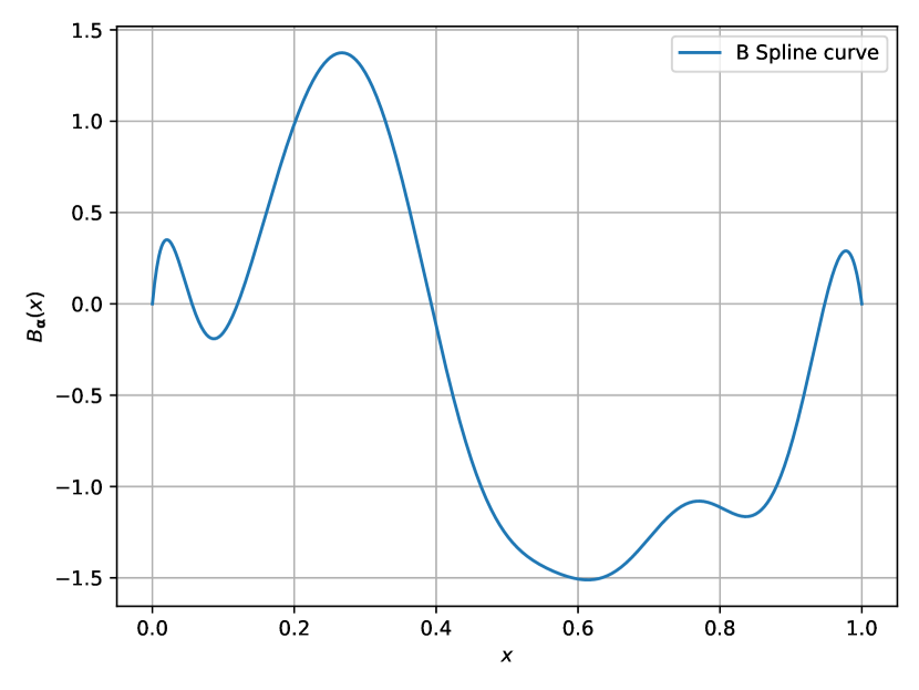
Figure 1: A B-Spline curve of degree $k=5$ with 14 B-Splines and random weights, except for the first and last, which were set to 0, to enforce the spline to be 0 at the boundaries

Our goal is to use B-Splines as a prior and the weights $\boldsymbol{\alpha}$ as shape parameters. We could also use the knot positions t as additional shape parameters to increase the model’s flexibility but did not do so in our current implementation. To achieve this, we need the B-Spline curve to be normalized or square normalized, respectively. We will start with the normalized case:

2.3.1 M-Splines

The basic idea for a normalized B-Spline curve is to normalize every B-Spline individually $\int B_{i,k}(x|\textbf{t})\text{d}x=1$ and then make sure that the weights sum up to 1: $\sum\alpha_{i}=1$ and are positive: $\alpha_{i}\geq 1\forall i\in\{0,...,N\}$. The B-Spline basis fulfilling the normalization requirement is called the M-Splines basis (Ramsay, 1988; Curry & Schoenberg, 1988) and has a formula closely related to B-Splines:

$$\begin{split}M_{i,1}(x|\textbf{t})&=\begin{cases}\frac{1}{t_{i+1}-t_{i}},&t_{i}<x<t_{i+1};\\ 0,&\text{otherwise}.\end{cases}\\ M_{i,k}(x|\textbf{t})&=\frac{k}{(k-1)(t_{i+k}-t_{i})}[(x-t_{i})M_{i,k-1}(x|\textbf{t})+\\ &\quad(t_{i+k}-x)M_{i+1,k-1}(x|\textbf{t})].\end{split}$$ (7)

Enforcing positivity and normalization of $\boldsymbol{\alpha}$ can be done by taking the softmax over the outputs of our neural network. An example of an M-Spline curve is shown in figure 2, where we can see that the spline can easily represent distributions with disconnected modes.
We sample $M_{\boldsymbol{\alpha}}(x)$ with rejection sampling. To do so, we need an upper bound for the max value of $M_{\boldsymbol{\alpha}}(x)$, which we give in the following theorem (proof in appendix A.4).

Theorem 1.

The max value of an M-Spline curve $M_{\boldsymbol{\alpha}}(x)$ of degree $k$ is bounded by

$$\max{M_{\boldsymbol{\alpha}}(x|\textbf{t})}\leq k\max_{i}{\max_{x}{M_{i,k}(x|\textbf{t})}}.$$ (8)

Note that we only sample one dimension at a time. Therefore, rejection sampling is very efficient. The double max on the RHS can be found numerically by precomputing the basis once before training, as long as t is constant.

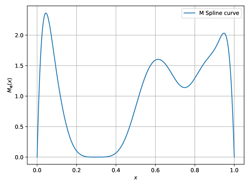
Figure 2: M-Spline curve with disconnected modes.

2.3.2 O-Splines

Next, we consider the square normalized case. We want

$$\begin{split}&\int\left(\sum_{i=0}^{N}\alpha_{i}B_{i,k}(x|\textbf{t})\right)^{2}\\ &=\int\sum_{i=0}^{N}\sum_{j<i}^{N}\alpha_{i}\alpha_{j}B_{i,k}(x|\textbf{t})B_{j,k}(x|\textbf{t})\stackrel{{\scriptstyle!}}{{=}}1.\end{split}$$ (9)

To enforce this, we symmetrically orthogonalize the B-Spline basis using Löwdings symmetric orthogonalization (Löwdin, 1956). These splines are also known as O-Splines (even though the name O-Spline can also refer to different orthogonalization schemes). Since the orthogonalization is performed nummerically once before training, we can only use the weights, not the knot positions, as shape parameters. A visualization of the O-Splines is depicted in the appendix (figure 11). Using these O-Splines $O_{i,k}(x)$ equation (10) becomes:

$$\int\left(\sum_{i=0}^{N}\beta_{i}O_{i,k}(x|\textbf{t})\right)^{2}=\int\sum_{i=0}^{N}\beta_{i}^{2}O_{i,k}^{2}(x|\textbf{t})=1.$$ (10)

Thus, it is enough to make every $O_{i,k}(x)$ individually square normalized, so $\int O_{i,k}^{2}(x|\textbf{t})=1$, which again can be done once before training. We also need to enforce $\sum\beta_{i}^{2}=1$ using the transformation

$$\text{sn}(\beta_{i};\beta_{0},...,\beta_{N})=\frac{\beta_{i}}{\sqrt{\sum_{j=0}^{N}\beta_{j}^{2}}}.$$ (11)

Next, to sample $O_{\boldsymbol{\beta}}(x)^{2}$ with rejection sampling, we need the max value, which is given by the following theorem

Theorem 2.

The max value of a O-Spline curve $O_{\boldsymbol{\beta}}(x)^{2}$ is bounded by

$$O_{\boldsymbol{\beta}}(x)^{2}\leq\max_{i}{(\boldsymbol{\beta}M_{O\rightarrow B})^{2}},$$ (12)

where $M_{B\rightarrow O}$ denotes the basis change matrix from the B-Spline basis to the O-Spline basis, and the maximum goes over the entries of the vector.

The proof for theorem 2 is presented in appendix A.6.

2.4 I-Splines

One of the most successful bijections $g^{-1}(x)$ for normalizing flows are monotonic splines, for example, the rational quadratic spline (RQS) bijection (Durkan et al., 2019). However, RQS are only differentiable once though. In many physics applications, however, we want more than the first derivative to exist, as the derivative itself is a meaningful quantity. For example, in our case, we need at least the second derivative to exist since we have to take the Laplacian of the function to train the model (see section 2.6). Some bijections are smooth enough, for example, mixture of logistic transformations (Ho et al., 2019), deep (dense) sigmoidalflows (Huang et al., 2018) and smooth bump functions (Köhler et al., 2021); however, due to the success and fine-grained control of previous spline bijections we propose to use I-Spline bijections. I-Spline curves are integrated M-Spline curves (Curry & Schoenberg, 1988; Ramsay, 1988):

$$I_{\boldsymbol{\alpha}}(x|\textbf{t})=\int_{0}^{x}\sum_{i=0}^{N}\alpha_{i}M_{i,k}(y|\textbf{t})\text{d}y,$$ (13)

with the same normalization conditions on the weights. Since M-Splines are positive, the integral is monotonically increasing, as desired (see figure 10 in the appendix for I-Splines and 3 for an I-Spline curve).

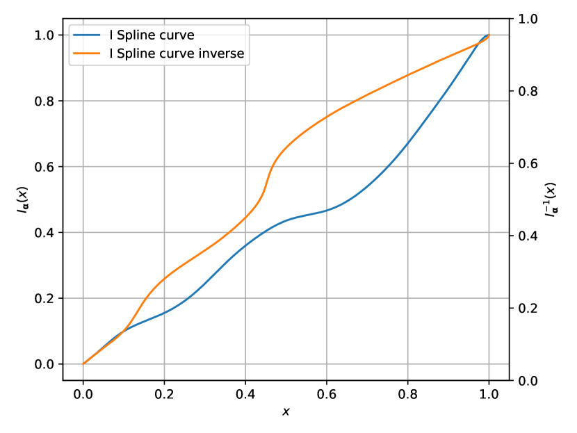
Figure 3: An I-Spline curve of degree $k=5$ with 14 I-Splines and random weights, except for the first and last which were set to 0, to enforce the spline to go from 0 to 1 at the boundaries.

We can also choose how smooth we want the I-Spline to be since it will always be one time more differentiable than the M-Spline it is based on.
Unlike RQS, we don’t have an analytical inverse available. Instead, we use binary search to find the inverse up to a small numerical error. Since calling the I-Spline function is very cheap compared to NN calls, inverting the I-Spline does not introduce a computational bottleneck.
Since the numerical inversion can become unstable for very flat areas of the I-Spline curve, we can explicitly regularize the minimal derivative by adding a small constant $\epsilon_{\text{regularize}}$ to all weights before we normalize them. Currently, we are only using the weights as free parameters predicted by our NN. Similar to the prior distribution, we could increase the flexibility by also predicting the knot positions, though.

2.5 Enforcing boundary conditions

Next, we show how we can enforce a certain limited class of boundary conditions for both normalizing and square normalizing flows:

$$p(x_{0},...,x_{i}=x^{*},....,x_{n-1})=0,$$ (14)

$$\partial_{x_{i}}p(x_{0},...,x_{i},....,x_{n-1})_{|x_{i}=x^{*}}=0,$$ (15)

$$\partial^{2}_{x_{i}}p(x_{0},...,x_{i},....,x_{n-1})_{|x_{i}=x^{*}}=0,$$ (16)

where we call $x^{*}$ the enforcement point. In the future, we might be able to extend this idea to enforce a wider range of boundary conditions. We will start with condition (14). Condition (15) and (16) follow similar ideas but are more complicated and not needed for our current application, so we will discuss them in the appendix A.7.

Theorem 3.

Let $g^{-1}_{i}(\textbf{x})$ be a composition of autregressive bijections with parameter functions $\boldsymbol{\theta}_{l}$ as defined in the main text, and let $g^{-1}(x_{i}=x^{*}|\boldsymbol{\theta}_{l}(x_{0:i-1}))=x^{*}\forall l\land\boldsymbol{\theta}$, and let $p_{\textbf{z}}(\textbf{z})$ be an autoregressive prior distribution with $p_{z}(z_{i}=x^{*}|\text{SP}(x_{:i-1}))=0\forall\text{SP}$. Then any (square) normalizing flow as defined in (4) full fills $p_{\textbf{x}}(x_{0},...,x_{i}=x^{*},...,x_{n-1})=0$.

The proof is in appendix A.7.1. The preconditions of theorem 3 can easily be fulfilled by just forcing the M/O/I-Splines to have the desired values at $x^{*}$ (this fine-grained control is another major benefit of spline-based bijections).

2.6 Variational Quantum Monte Carlo

In this section, we briefly introduce variational quantum Monte Carlo (VQMC) (Toulouse et al., 2015), a widely used framework to approximate the ground state energy of a given Hamiltonian $\hat{H}$. Suppose the system is described by a square normalized wave function $\psi_{\boldsymbol{\theta}}(\textbf{x})$, then the energy of the system is expressed as the expectation value of $H$

$$\begin{split}E(\boldsymbol{\theta})=\int\psi^{*}_{\boldsymbol{\theta}}(\textbf{x})H\psi_{\boldsymbol{\theta}}(\textbf{x})\ \mathrm{d}\textbf{x}=\int|\psi_{\boldsymbol{\theta}}(\textbf{x})|^{2}\underbrace{\frac{H\psi_{\boldsymbol{\theta}}(\textbf{x})}{\psi_{\boldsymbol{\theta}}(\textbf{x})}}_{E^{L}_{\boldsymbol{\theta}}(\textbf{x})}\mathrm{d}\textbf{x}\end{split}$$ (17)

which we can approximate with samples from $|\psi_{\boldsymbol{\theta}(x)}|^{2}$. The ground state energy $E_{0}$ is the lowest energy that the system can reach and can be approximated by minimizing $E(\boldsymbol{\theta})$ with respect to $\boldsymbol{\theta}$

$$\begin{split}E_{\text{VQMC}}=\min_{\boldsymbol{\theta}}E(\boldsymbol{\theta}).\end{split}$$ (18)

We then solve (18) using gradient descent with respect to the parameters $\theta$ of the Ansatz (see the appendixA.8 for a derivation):

$$\begin{split}\nabla_{\theta}&\int|\psi_{\boldsymbol{\theta}}(\textbf{x})|^{2}E^{L}_{\boldsymbol{\theta}}(\textbf{x})\ \mathrm{d}\textbf{x}=\\ &\operatorname*{\mathbb{E}}_{|\psi_{\boldsymbol{\theta}}(\textbf{x})|^{2}}\left(\nabla_{\theta}\log(|\psi_{\boldsymbol{\theta}}(\textbf{x})|^{2})E^{L}_{\boldsymbol{\theta}}(\textbf{x})\ +\nabla_{\theta}E^{L}_{\boldsymbol{\theta}}(\textbf{x})\right)\\ \end{split}$$ (19)

2.7 Electronic wave functions

A many-electron wave function $\Psi(\mathbf{r}_{0},\mathbf{r}_{1},\cdots,\mathbf{r}_{n-1})$ is a complex function used to describe the quantum state of $n$ electrons. While the concept of the wave function is rather abstract, the square of its absolute value has a physical meaning. Let $\rho(\mathbf{r}_{0},\mathbf{r}_{1},\cdots,\mathbf{r}_{n-1})=|\Psi(\mathbf{r}_{0},\mathbf{r}_{1},\cdots,\mathbf{r}_{n-1})|^{2}$, then $\rho(\mathbf{r}_{0},\mathbf{r}_{1},\cdots,\mathbf{r}_{n-1})$ represents the probability of finding electron-1 at $\mathbf{r}_{0}$, electron-2 at $\mathbf{r}_{1}$, and so on, and

$$\begin{split}\int\mathrm{d}\mathbf{r}_{0}\mathrm{d}\mathbf{r}_{1}\cdots\mathrm{d}\mathbf{r}_{n-1}\rho(\mathbf{r}_{0},\mathbf{r}_{1},\cdots,\mathbf{r}_{n-1})=1.\end{split}$$ (20)

Therefore, the electronic wave function $\Psi(\mathbf{r}_{0},\mathbf{r}_{1},\cdots,\mathbf{r}_{n-1})$ is square normalized.

Note that here $\mathbf{r}_{i}$ should be interpreted as a general coordinate of electron-$i$. A common choice of $\mathbf{r}_{i}$ is to include both the spin and spatial coordinates of the electron. Electrons are spin-$\frac{1}{2}$ particles (Mann, 2010; Schwartz, 2013), which means that an electron can have two spin freedoms: spin-up or spin-down. In most electronic structure problems, the wave functions of electrons with different spins can be separated, and the wave function of the whole system is a direct product of wave functions with different spins. In the following, we will assume that all electrons are spin-up and focus our effort on studying the wave function with respect to the spatial coordinates $\mathbf{x_{i}}$. We use $\psi(\mathbf{x}_{1},\mathbf{x}_{2},\cdots,\mathbf{x}_{n})$ to represent a wave function that only depends on the spatial coordinates.

Another unique property of electrons is antisymmetry, which means that when exchanging two electrons, the wave function will gain an opposite sign:

$$\begin{split}\psi(&\mathbf{x}_{0},\cdots,\mathbf{x}_{i},\cdots,\mathbf{x}_{j},\cdots,\mathbf{x}_{n-1})=\\ &-\psi(\mathbf{x}_{0},\cdots,\mathbf{x}_{j},\cdots,\mathbf{x}_{i},\cdots,\mathbf{x}_{n-1}),\hskip 10.00002pti\neq j\end{split}$$ (21)

The antisymmetric nature of electrons described in Eq.(21) is the main cause of simulation difficulties in the modern electronic structure theory, causing unfavourable cubic scaling from the slater determinant and the infamous sign problem. In the next section, we aim to construct many-electron wave functions that satisfy the antisymmetric property by defining the wave function only on the fundamental domain.

2.8 The fundamental domain

As described in section 2.7, a fermionic wave function needs to be antisymmetric. If we do not enforce this symmetry onto our Ansatz, we can get lower energies than would be found in nature, and we cannot train the model with the VQMC objective anymore. Unfortunately, the usual way of enforcing antisymmetry, using the slater determinant, does not work for normalizing flows since the functional form of normalizing flows does not permit addition or subtraction. We are getting around this issue by only training the model on the fundamental domain of the permutation operator and enforcing the necessary boundary conditions (Klimyk et al., 2007). To define the fundamental domain, let us first define the orbit of a point under a group as:

Definition 2.1 (Orbit).

Let $G$ be a group that acts on a space $X$. Then we define the orbit of a point $x\in X$ as $\text{Orb}_{G}(x):=\{g\cdot x|g\in G\}$

Then we can define the fundamental domain of $G$ as:

Definition 2.2 (Fundamental Domain).

Let $G$ be a group that acts on a space $X$, and let $S\subset X$ be a closed subset of $X$. Then we call $S$ the fundamental domain of $G$ if

$$X=\cup_{x\in S}\text{Orb}_{G}(x)$$ (22)

and

$$\emptyset=\text{Orb}_{G}(x)\cap\text{Orb}_{G}(y)\forall x,y\in S.$$ (23)

Intuitively, $S$ is the "symmetry cell" of a symmetry group, so we can reach any other point in $X$ just by applying symmetry operations. Put yet another way, by defining a (anti)symmetric function on its fundamental domain, it is defined for the entire space.
Let us now get specific and consider the fundamental domain of the group P of permutation operators $P_{\sigma}$ that act on a function $\psi(x_{0},x_{1},...,x_{n-1})$ the following way

$$P_{\sigma}\psi(x_{0},x_{1},...,x_{n-1})=\psi(\sigma(x_{0}),\sigma(x_{1}),...,\sigma(x_{n-1})),$$ (24)

where $\sigma$ represents a specific permutation. Then the fundamental domain of P is given by:

Theorem 4.

$S=\{x_{0}\leq x_{1}\leq....\leq x_{n-1}\|x_{0},...,x_{n-1}\in\mathbb{R}\}$ is a fundamental domain of P on $\mathbb{R}^{n}$

In other words, we pick one specific ordering of the dimensions. It is clear that any other ordering can be reached by permuting the dimensions. Thus, $S$ is a fundamental domain of P. In 2.7, we have described that a fermionic wave function needs to be antisymmetric. If we want to define our wave function only on the fundamental domain, to make it continous we have to impose the additional boundary condition (Klimyk et al., 2007):

$$\psi(\textbf{x})=0\forall\textbf{x}\in\partial S,$$ (25)

where $\partial S$ denotes the boundary of the fundamental domain, which is reached whenever two coordinates coincide. Physically equation (25) means that two identical particles cannot be found at the same location in space.
To get a better intuitive understanding of our setup, we can look at the simplest imaginable system: Two fermions in a box in their groundstate, which can be analytically written as:

$$\begin{split}\psi(x_{0},x_{1})=\frac{1}{\sqrt{2}}\left(\frac{2}{L}\sin{\left(\frac{\pi x_{0}}{L}\right)}\sin{\left(\frac{2\pi x_{1}}{L}\right)}-\right.\\ \left.\sin{\left(\frac{\pi x_{1}}{L}\right)}\sin{\left(\frac{2\pi x_{0}}{L}\right)}\right).\end{split}$$ (26)

We plot this function in figure 4 and mark the fundamental domain.

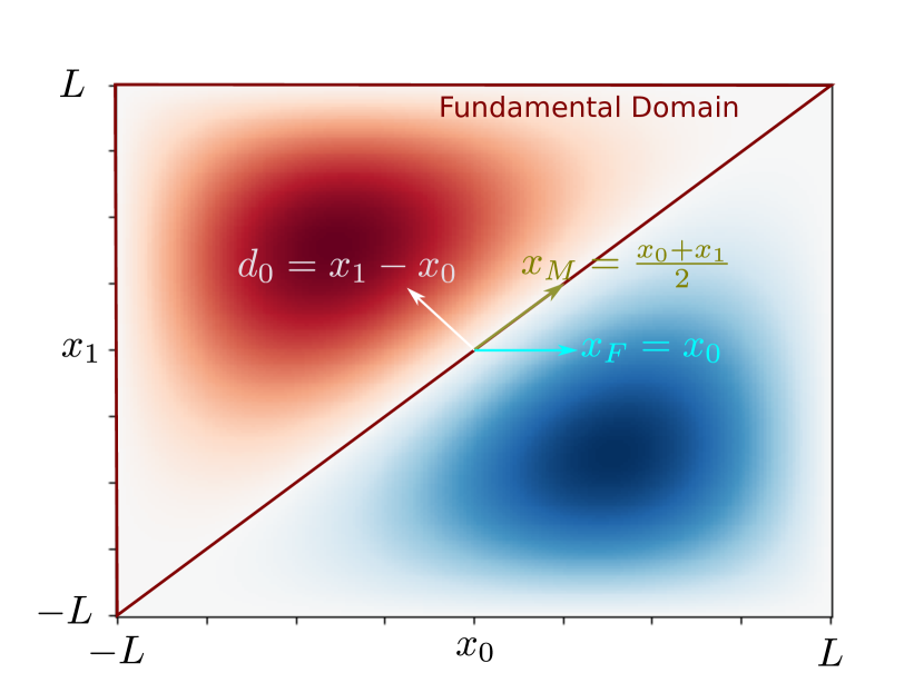
Figure 4: Plot of the wave function of two particles in a box, and the relative coordinate system and fundamental domain visualized. Note, the fundamental domain is not unique, but all of them (here two) are equivalent.

2.9 Waveflow

In this section, we combine the techniques described above to describe Waveflow. For now, we restrict ourselves to spatially one-dimensional, multi-particle systems. We also impose the technical restriction that the system is always contained in a box of size $2L$ (see figure 5). However, this restriction is unimportant for most systems, as we can make the box arbitrarily large.

To enforce antisymmetry, we learn the wave function only on one fundamental domain and enforce condition (25). For this, we change the coordinate system from absolute coordinates $\{x_{0},...,x_{n-1}\}$ to relative coordinates $\{d_{i}=x_{i+1}-x_{i}|i\in\{0,...,n-2\}\}$. The $i-1$ relative coordinates describe how the particles relate to each other, leaving one extra unconstrained coordinate $x_{u}$ that describes where the particle system is globally. We tried two choices for $x_{u}$, the mean of the absolute coordinates, denoted by $x_{M}$, and $x_{F}$, the absolute coordinate of the first particle (see figure 5 for a visual explanation). It is easy to see that in this new coordinate system, the fundamental domain is given by $\{d_{0},...,d_{n-2},x_{u}|d_{i}\in\mathbb{R}^{+}\forall i,x_{u}\in\mathbb{R}\}$.
Since our I-Splines are mapping from [0,1] to [0,1], we also need to scale all coordinates into the [0,1] range. For the relative coordinates, 0 means that two particles are coinciding, and 1 means that the particle is at the end of the box. For $x_{F}$ both 0 and 1 correspond to the box’s walls, and for $x_{M}$ both 0 and 1 correspond to the allowable regions the mean could be in, given the relative coordinates.

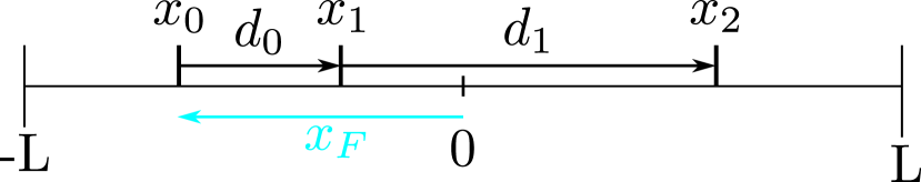
(a) Relative coordinates with $x_{u}=x_{F}=x_{0}$.

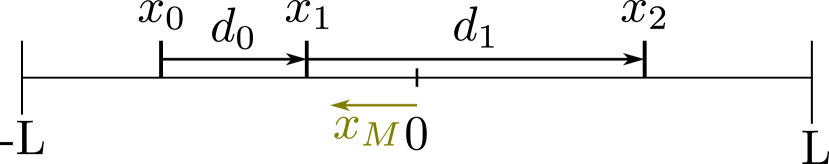
(b) Relative coordinates with $x_{u}=x_{M}=\frac{x_{0}+...+x_{n-1}}{n}$

Figure 5: Example system of three one-space dimensional particles in a box described in absolute coordinates $x_{0},x_{1},x_{2}$ and in a relative coordinate system $d_{0},d_{1},x_{u}$ for the two different choices of unconstrained coordinates.

Both coordinate systems (including scaling) can be constructed as flow layers. We can therefore incorporate the coordinate transformations as parameter-free first layers in our square normalizing flow. The details are described in algorithm 6 and 8 in the appendix.
To enforce the boundary conditions (25) we now have to make sure that $\psi(d_{0},...,d_{n-2},x_{u})=0$ if $d_{i}=0$ for any $i$. Since a box constrains the particle system, the wave function also needs to be 0 if any of the particles are on the wall of the box. Since we scaled everything to be in [0,1], at least one particle is on the wall if $d_{i}=1$ or $x_{u}=0$ or $x_{u}=1$. Thus the overall constraints we want to enforce on our wave function ansatz are

$$\begin{split}\psi(d_{0},...,d_{i}=0,...d_{n-2},x_{u})&=0\ \forall i,\\ \psi(d_{0},...,d_{i}=1,...d_{n-2},x_{u})&=0\ \forall i,\\ \psi(d_{0},...,d_{n-2},x_{u}=0)&=0,\\ \psi(d_{0},...,d_{n-2},x_{u}=1)&=0,\end{split}$$ (27)

which we do using theorem 3. We can then train the Waveflow Ansatz using vqmc by drawing samples from our Ansatz.
Finally, if we want to evaluate $\psi(x_{0},...,x_{n-1})$ outside of the fundamental domain, first we sort the coordinates to map back into our fundamental domain and then multiply by $-1^{IC(x_{0},...,x_{n-1})}$, where $IC(x_{0},...,x_{n-1})$ is the inversion count of the sorting:

$$\begin{split}\psi(x_{0},...,x_{n-1})=-1^{IC(x_{0},...,x_{n-1})}\psi(d_{0},...,d_{n-2},x_{u})\end{split}$$ (28)

Note, however, that we only need equation (28) for visualization purposes, not training.

3 Experiments

We are testing our method on a simple toy example: Two electrons in a helium potential. As is common for one-dimensional systems, we are using the soft Coulomb potential $u(x)=\frac{1}{\sqrt{1+x^{2}}}$. We can write the Hamiltonian as

$$H=-\frac{1}{2}\Delta-\frac{2}{u(x_{0})}-\frac{2}{u(x_{1})}+\frac{1}{u(x_{0}-x_{1})}$$ (29)

We use a Waveflow Ansatz with the spline degree $k=5$, 23 knots and 3 I-Spline bijection layers and $x_{u}=x_{M}$. We optimize the network using the Adam optimizer (Kingma & Ba, 2014) with a learning rate $10^{-4}$ and a batch size of 128. The box had a length of $L=10$. The MADE network has one hidden layer with 64 neurons in each layer. We train the model for 60000 epochs which takes about 10 minutes on an Nvidia GeForce RTX 2070. None of these hyperparameters were optimized; they represent our first guess. Using the QMsolve library (Rafael de la Fuente, 2022), we determine the groundtruth solution, which is plotted in figure 6(a).

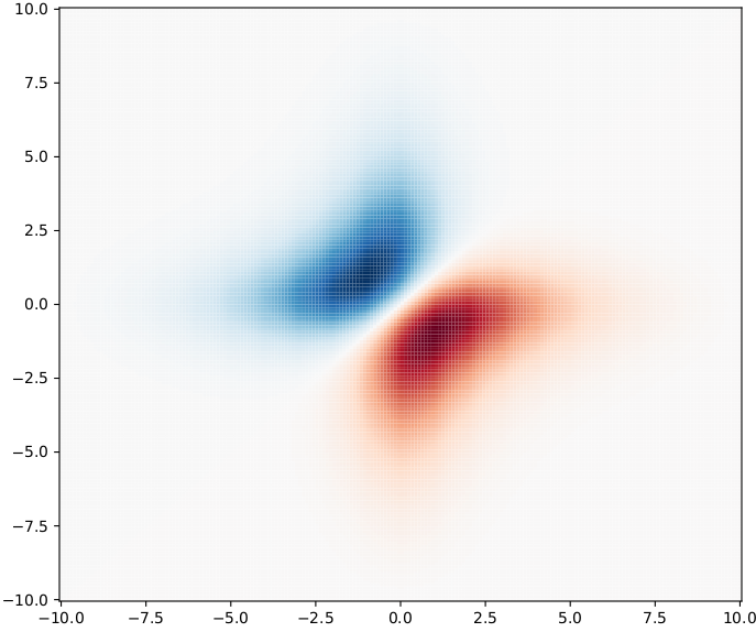
(a) QMSolve

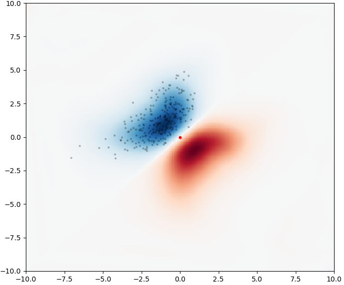
(b) Waveflow

Figure 6: Comparison of the antisymmetric groundstate of Hamiltonian (29) obtained with QMSolve and Waveflow respectively. We see that Waveflow learns the groundstate correctly.

When we compare this to figure 6(b), we see that the result of Waveflow looks very similar. In the appendix, we also plot the training progression 12, making it obvious that Waveflow overcame the topology problem. We can also compare the energy values from QMsolve and Waveflow, which are given in table 1: Waveflow is very close to the ground truth and well within the error bounds of Waveflow’s prediction.

Method	Energy (in Hartree)
QMsolve	$-1.8125$
Waveflow	$-1.803\pm 0.025$

Table 1: The energy values obtained from the QMsolve library and Waveflow. We can see that the ground truth energies are well within the error interval predicted by Waveflow. The energy and variance for Waveflow were obtained using a running variance estimate of the last 5000 epochs.

Code for our experiments will be available at: <github>

4 Conclusion

In this work, we took steps towards a very efficient normalizing flow ansatz for vqmc simulations of electrons. We enforce the anti-symmetry of the wave function by defining and training it only on the fundamental domain of the permutation group and then enforcing boundary conditions on our ansatz. To make this work, we developed several new techniques for normalizing flows that might be of broader interest to the ML-for-science community. While this work focused on introducing the technical aspects of Waveflow and showed a proof-of-principle of its components on a simple toy problem, in future work, we plan to scale our approach to bigger systems with more particles. The biggest open challenge, however, is to expand our approach to three space dimensions, which seems difficult but not hopeless. If we succeed in this, the payoff could be huge, as it could help scale vqmc methods to much bigger systems.

Appendix A Appendix

A.1 Normalizing Flow algorithm

This section presents the pseudocode to evaluate 1 and to sample 2 a standard normalizing flow. The same algorithms can be used for square normalizing flows by replacing $p_{z}(z)$ with $\psi_{z}(z)$ and det with $\sqrt{\text{det}}$ in the last line of 1 for evaluation, and sample from $\psi_{z}^{2}(x)$ instead of $p_{z}(z)$ in 2.

Algorithm 1 Evaluating an autoregressive Normalizing Flow

  Input: x, $\text{det}=0$, a simple prior distribution $p_{z}(z)$, NN parameter

  Output: $p_{\textbf{x}}(\textbf{x})=p_{\textbf{z}}(g^{-1}(\textbf{x}))\cdot|\text{det}{\,\textbf{J}\left(g^{-1}(\textbf{x})\right)}|$

  Initialize $\text{det}=1$

  for $l$=0,…L-1 do

     $\boldsymbol{\theta}_{l}=\boldsymbol{\theta}_{l}(\textbf{x})$

     for $i=0...n-1$ do

        $x^{l+1}_{i}=g^{-1}(x_{i}|\boldsymbol{\theta}_{i})$

        $\text{det}=\text{det}\cdot\partial_{x}g^{-1}(x_{i}|\boldsymbol{\theta}_{i})$

     end for

  end for

  return $p_{\textbf{x}}(\textbf{x})=\prod_{i=0}^{n}p_{z}(x_{i}^{L})\cdot\text{det}$

Algorithm 2 Sampling an autoregressive Normalizing Flow

  Input: NN parameter

  Output: $\textbf{x}\sim p_{\textbf{x}}(\textbf{x})$

  Draw a sample from the prior $\textbf{x}^{L}\sim p_{\textbf{z}}(\textbf{z})$

  for $l$=L-1,…0 do

     for $i=0...n-1$ do

        $\boldsymbol{\theta}_{i}=\boldsymbol{\theta}_{l}(x^{l}_{i=0,...,i-1})$

        $x^{l}_{i}=g(x_{i}|\boldsymbol{\theta}_{i})$

     end for

  end for

  return $\textbf{x}^{0}$

With our modifications described in the main body of the paper, the algorithms become:

Algorithm 3 Evaluating an autoregressive Normalizing Flow with adaptive prior

  Input: x, $\text{det}=0$, a simple prior distribution $p_{z}(z)$, NN parameter

  Output: $p_{\textbf{x}}(\textbf{x})=p_{\textbf{z}}(g^{-1}(\textbf{x}))\cdot|\text{det}{\,\textbf{J}\left(g^{-1}(\textbf{x})\right)}|$

  Initialize $\text{det}=1$

  for $l$=0,…L-1 do

     $\boldsymbol{\theta}_{l}=\boldsymbol{\theta}_{l}(\textbf{x})$

     for $i=0...n-1$ do

        $x^{l+1}_{i}=g^{-1}(x_{i}|\boldsymbol{\theta}_{i})$

        $\text{det}=\text{det}\cdot\partial_{x}g^{-1}(x_{i}|\boldsymbol{\theta}_{i})$

     end for

  end for

  $\textbf{SP}=\textbf{SP}(\textbf{x})$

  return $p_{\textbf{x}}(\textbf{x})=\prod_{i=0}^{n}p_{z}(x_{i}^{L}|\textbf{SP}_{i})\cdot\text{det}$

Algorithm 4 Sampling an autoregressive Normalizing Flow with adaptive prior

  Input: NN parameter

  Output: $\textbf{x}\sim p_{\textbf{x}}(\textbf{x})$

  Draw a sample from the adaptive prior: $x_{0}^{L}\sim p_{z}(z|\textbf{SP}_{0})$

  for $i=0...n-1$ do

     $\textbf{SP}_{i}=\textbf{SF}(x^{l}_{i=0,...,i-1})$

     $x^{L}_{i}\sim p_{z}(z|\textbf{SP}_{i})$

  end for

  Transform the sample:

  for $l$=L-1,…0 do

     for $i=0...n-1$ do

        $\boldsymbol{\theta}_{i}=\boldsymbol{\theta}_{l}(x^{l}_{i=0,...,i-1})$

        $x^{l}_{i}=g(x_{i}|\boldsymbol{\theta}_{i})$

     end for

  end for

  return $\textbf{x}^{0}$

A.2 The topology problem visualized

The topology problem of normalizing flows refers to the problem, that a continious coordinate transform cannot change the topology of the prior. For example, consider a gaussian that ought to be transformed into two disconnected halfmoons. Then there will always remain some small connection, see 7. While this connection can be made arbitrarily small, this can provably lead to nummerical problems during sampling of the model (Cornish et al., 2020).

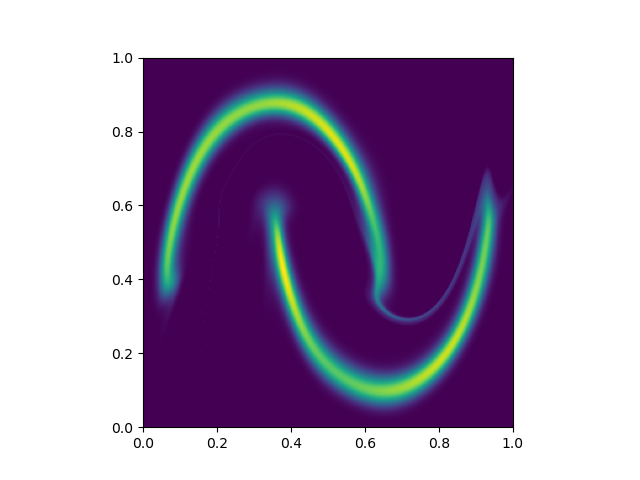
Figure 7: A gaussian that was transformed into a halfmoon distribution using a simple MADE (Germain et al., 2015). Since a gaussian has only one connected mode, the flow cannot easily separate it into two disconnected modes.

For square normalizing flows, where we the prior has positive and negative areas in the function, and nodes where the function switches between them, the problem is not just numerical instability. The topology problem in this context means, that the flow cannot create or destroy nodes (see figure 8). Since the number of nodes can strongly influence the energy of a Wavefunction (Ceperley, 1991), this is a big problem.

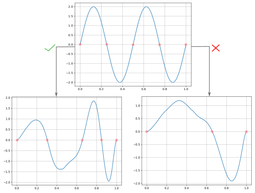
Figure 8: Conceptual depiction of how a simple sine wavefunction can be transformed into a new one. The topology must be preserved, that means, the number of of nodes (red) needs to stay constant. Bottom left: An allowed transformation. Bottom right: A disallowed transformation

A.3 B-Splines

B-Splines have some important properties that we can use to estimate the maximum values of the splines:

1. Local support property: Any B-Spline basis $B_{i,k}(x)$ has support on exactly $k$ consecutive knot points and is zero outside this interval. Also reversely, each knot affects exactly $k$ bases. This means specifically also, that every weight $\alpha_{i}$ only affects $B_{\boldsymbol{\alpha}}(x)$ only on the interval $t_{i}<t<t_{i+k}$

2. Two useful properties are $B_{i,k}(x)\geq 0$ and $\sum_{i}B_{i,k}(x)=1$

For reference, figure 9 shows B-Splines for $N=14$ and $k=5$.

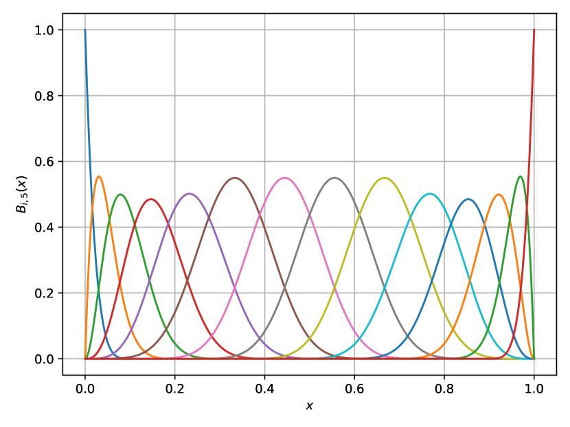
Figure 9: 14 B-Splines of degree $k=5$

A.4 M-Spline details

Here we will give a proof of theorem 1:

Theorem 1.

The max value of an M-Spline curve $M_{\boldsymbol{\alpha}}(x)$ of degree $k$ is bounded by

$$\begin{split}\max{M_{\boldsymbol{\alpha}}(x|\textbf{t})}\leq k\max_{i}{\max_{x}{M_{i,k}(x|\textbf{t})}}.\end{split}$$ (30)

Proof.

M-Splines possess the same local support property as described for B-Splines in A.3. Therefore, for every $x$ we only have to consider the $k$ $B_{i,k}(x)$ that are non-zero. We also know that $\alpha_{i}\leq 1\forall i$. Therefore there exists a $j$ such that we we can write

$$\begin{split}M_{\boldsymbol{\alpha}}(x|\textbf{t})&=\sum_{i}^{N}\alpha_{i}M_{i,k}(x|\textbf{t})=\sum_{i=j}^{j+k}\alpha_{i}M_{i,k}(x|\textbf{t})\\ &\leq\sum_{i=j}^{j+k}M_{i,k}(x|\textbf{t})\leq\sum_{i=j}^{j+k}\max_{x}{M_{i,k}(x|\textbf{t})}\\ &\leq k\max_{i}\max_{x}M_{i,k}(x|\textbf{t})\end{split}$$ (31)

∎

A.5 I-Splines

I-Splines are just integrated M-Splines. Since M-Splines are strictly positive, their integration is monotonically increasing. Figure 10 shows an example for I-Splines with $k=5$.

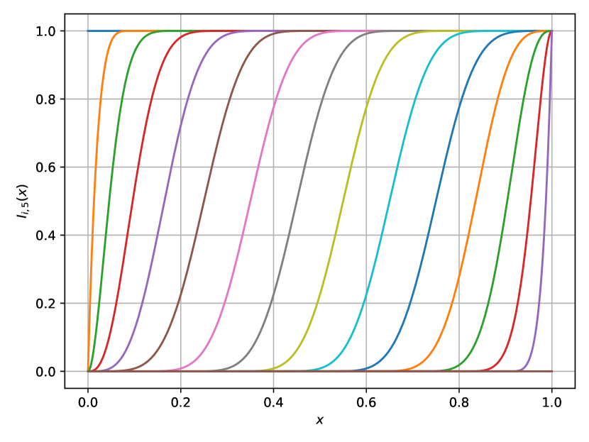
Figure 10: 14 I-Splines of degree $k=5$

A.6 O-Spline details

For two vectors $\mathbf{v}_{1}$ and $\mathbf{v}_{2}$, we use the following equations to perform Löwdin orthogonalization(Löwdin, 1956),

$$\begin{split}\mathbf{o}_{1}&=\frac{1}{2}\left(\frac{\mathbf{v}_{1}}{\sqrt{1+\mathbf{v}_{1}\cdot\mathbf{v}_{2}}}+\frac{\mathbf{v}_{2}}{\sqrt{1-\mathbf{v}_{1}\cdot\mathbf{v}_{2}}}\right),\\ \mathbf{o}_{2}&=\frac{1}{2}\left(\frac{\mathbf{v}_{1}}{\sqrt{1-\mathbf{v}_{1}\cdot\mathbf{v}_{2}}}+\frac{\mathbf{v}_{2}}{\sqrt{1+\mathbf{v}_{1}\cdot\mathbf{v}_{2}}}\right).\end{split}$$ (32)

For more vectors $\{\mathbf{v}_{1},\cdots,\mathbf{v}_{N}\}$, we perform the above procedure to pairwise diagonalize the vectors: $\mathbf{v}_{1},\mathbf{v}_{N}\rightarrow\mathbf{o}_{1},\mathbf{o}_{N}$, $\mathbf{v}_{2},\mathbf{v}_{N-1}\rightarrow\mathbf{o}_{2},\mathbf{o}_{N-1}$, etc.

The algorithm (Liu et al., 2019) is summarized in Algorithm 5. Note that all the indices in the algorithm start from $1$ instead of $0$.

Algorithm 5 Symmetrized Gram-Schmidt orthogonalization

  Input: Matrix $A$ - columns of which are the input vectors $\{\mathbf{v}_{1},\cdots,\mathbf{v}_{N}\}$.

  Output: Matrix $B$ - columns of which are the symmetrically orthogonalized vectors.

  $n_{p}=\lfloor N/2\rfloor$.

  Reshuffle the vectors in matrix $A$ into two matrices $A_{L}$ and $A_{R}$.

  if $N$ is even then

     $A_{L}=\{\mathbf{v}_{1},\mathbf{v}_{2n_{p}},\mathbf{v}_{2},\mathbf{v}_{2n_{p}-1},\cdots,\mathbf{v}_{n_{p}},\mathbf{v}_{n_{p}+1}\}$,

     $A_{R}=\{\mathbf{v}_{2n_{p}},\mathbf{v}_{1},\mathbf{v}_{2n_{p}-1},\mathbf{v}_{2},\cdots,\mathbf{v}_{n_{p}+1},\mathbf{v}_{n_{p}}\}$.

  else

     $A_{L}=\{\mathbf{v}_{1},\mathbf{v}_{2n_{p}+1},\mathbf{v}_{2},\mathbf{v}_{2n_{p}},\cdots,\mathbf{v}_{n_{p}},\mathbf{v}_{n_{p}+2},\mathbf{v}_{n_{p}+1}\}$,

     $A_{R}=\{\mathbf{v}_{2n_{p}+1},\mathbf{v}_{1},\mathbf{v}_{2n_{p}},\mathbf{v}_{2},\cdots,\mathbf{v}_{n_{p}+2},\mathbf{v}_{n_{p}}\}$.

  end if

  Perform Gram-Schmidt orthogonalization to both matrices $A_{L}$ and $A_{R}$.

  if $N$ is odd then

     $B[:,n_{p}+1]=A_{L}[:,N]$.

  end if

  for $i=1,\dots,n_{p}$ do

     Pairwise diagonalization: $A_{L}[:,2*i-1],A_{R}[:,2*i-1]\rightarrow\mathbf{o}_{L},\mathbf{o}_{R}$ according to Eq. (32).

     $B[:,i]=\mathbf{o}_{L}$,

     $B[:,N-i+1]=\mathbf{o}_{R}$.

  end for

  return $B$

We plot $N=14$ O-Splines with $k=5$ in figure 11, that are obtained from orthogonalizing the splines in figure 9

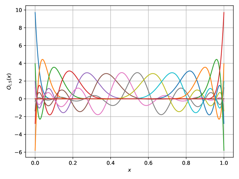
Figure 11: O-Splines obtain after Löwdings symmetric orthogonalization of the B-Splines in figure 9

Next we give the proof for theorem 2

Theorem 2.

The max value of a O-Spline curve $O_{\boldsymbol{\beta}}(x)^{2}$ is bounded by

$$\begin{split}O_{\boldsymbol{\beta}}(x|\textbf{t})^{2}\leq\max_{i}{\left((\boldsymbol{\beta}M_{O\rightarrow B})^{2}\right)}\end{split}$$ (33)

where $M_{B\rightarrow O}$ denotes the basis change matrix from the B-Spline basis to the O-Spline basis, and the maximum goes over the entries of the vector.

Proof.

Denote all O-Splines and B-Spline bases ordered in a vector as $\boldsymbol{O}(x|\textbf{t})$ and $\boldsymbol{B}(x|\textbf{t})$. Then we can write

$$\begin{split}&(O_{\boldsymbol{\beta}}(x|\textbf{t}))^{2}=(\boldsymbol{\beta}\boldsymbol{O}(x|\textbf{t}))^{2}=\left(\underbrace{\boldsymbol{\beta}M_{B\rightarrow O}}_{\boldsymbol{\alpha}}\boldsymbol{B}(x|\textbf{t})\right)^{2}\\ &=\left(\sum_{i}^{N}\alpha_{i}B_{i,k}(x|\textbf{t})\right)^{2}\leq\left(\max_{i}{|\boldsymbol{\alpha}|}\sum_{i}^{N}B_{i,k}(x|\textbf{t})\right)^{2}\\ &=\max_{i}{\boldsymbol{\alpha}^{2}}=\max_{i}{\left((\boldsymbol{\beta}M_{O\rightarrow B})^{2}\right)},\end{split}$$ (34)

where we used $\sum_{i}^{N}B_{i,k}(x|\textbf{t})=1$. ∎

A.7 Boundary condition details

In this section we detail the theorems for enforcing boundary condition 14 - 16 and the corresponding proofs. We use the following notation to reduce clutter in the proofs

$$\partial_{x_{i}}^{k}f(x_{0},...,x_{i},...,x_{n-1})=f^{(0,...,k,...0)}f(x_{0},...,x_{i},...,x_{n-1}).$$ (35)

A.7.1 First boundary condition

Theorem 3.

Let $g^{-1}_{i}(\textbf{x})$ be a composition of autoregressive bijections with parameter functions $\boldsymbol{\theta}_{l}$ as defined in the main text, and let $g^{-1}(x_{i}=x^{*}|\boldsymbol{\theta}_{l}(x_{0:i-1}))=x^{*}\forall l\land\boldsymbol{\theta}$, and let $p_{\textbf{z}}(\textbf{z})$ be an autoregressive prior distribution with $p_{z}(z_{i}=x^{*}|\text{SP}(x_{:i-1}))=0\forall\text{SP}$. Then any (square) normalizing flow as defined in 4 fulfills $p_{\textbf{x}}(x_{0},...,x_{i}=x^{*},...,x_{n-1})=0$.

Note that we can fulfill the preconditions of the theorem using M/O and I-Splines, since we can set the values of the spline at specified points to whatever we want.

Proof.

First note, that the bijections will map all points x with $\textbf{x}_{i}=x^{*}$ to new points x’ with $\textbf{x'}_{i}=x^{*}$ in every layer:

$$\begin{split}&g^{-1}(x_{i}=x^{*}|\boldsymbol{\theta}(x_{0:i-1}))\\ &=g^{-1}(x_{i}|\boldsymbol{\theta}_{L}(x_{0:i-1}^{L})\circ...\circ g^{-1}(x_{i}=x^{*}|\boldsymbol{\theta}_{0}(x_{0:i-1}^{0}))=x^{*}\end{split}$$ (36)

where $x^{l}$ indicates the transformed $x$ after $l$ layers. In the following we omit the shape parameters from the prior for readability. Then we get

$$p_{\textbf{x}}(x_{0},...,x_{i}=x^{*},...,x_{n-1})$$

$$=\ p_{z}(g^{-1}(x_{0}))\cdot...\cdot p_{z}(g^{-1}(x_{i}=x^{*}|x_{0:i-1}))\cdot...\cdot$$

$$\qquad p_{z}(g^{-1}(x_{n-1}|x_{0:n-2}))\cdot$$

$$\qquad\partial_{x_{0}}g^{-1}(x_{0})\cdot...\cdot$$

$$\qquad\partial_{x_{i}}g^{-1}(x_{i}=x^{*}|x_{0:i-1})\cdot...\cdot\partial_{x_{n-1}}g^{-1}(x_{n-1}|x_{0:n-2})$$

$$=\ p_{z}(g^{-1}(x_{0}))\cdot...\cdot\underbrace{p_{z}(x_{i}=x^{*})}_{=0}\cdot...\cdot p_{z}(g^{-1}(x_{n-1}|x_{0:n-2}))\cdot$$

$$\qquad\partial_{x_{0}}g^{-1}(x_{0})\cdot...\cdot$$

$$\qquad\partial_{x_{i}}g^{-1}(x_{i}=x^{*}|x_{0:i-1})\cdot...\cdot\partial_{x_{n-1}}g^{-1}(x_{n-1}|x_{0:n-2})$$

$$=\ 0.$$

∎

A.7.2 Second boundary condition

Theorem 4.

Let $g^{-1}_{i}(\textbf{x})$ be a composition of autoregressive bijections with parameter functions $\boldsymbol{\theta}_{l}$ as defined in the main text, and let $g^{-1}(x_{i}=x^{*}|\boldsymbol{\theta}_{l}(x_{0:i-1}))=x^{*}\land\partial_{x_{i}}^{2}g^{-1}(x_{i}|\boldsymbol{\theta}_{l}(x_{0:i-1}))|_{x_{i}=x^{*}}=0\forall l\land\boldsymbol{\theta}$, and let $\partial_{x_{i}}\boldsymbol{\theta}_{l}(x_{0:j})=0\forall l\land j\geq i$.
Furthermore, let $p_{\textbf{z}}(\textbf{z})$ be an autoregressive prior distribution with $\partial_{x_{i}}p_{z}(z_{i}=x^{*}|\text{SP}(x_{:j}))=0\forall\text{SP}\land j\geq i$ and let $\partial_{x_{i}}\text{SP}(x_{0:j})=0\forall l\land j\geq i$. Then any (square) normalizing flow as defined in 4 fulfills $\partial_{x_{i}}p_{\textbf{x}}(x_{0},...,x_{i}=x^{*},...,x_{n-1})=0$.

We can enforce the precondition that $\partial_{x_{i}}\boldsymbol{\theta}_{l}(x_{0:j})=0\forall l\land j\geq i$ and $\partial_{x_{i}}p_{z}(z_{i}=x^{*}|\text{SP}(x_{:j}))=0\forall\text{SP}\land j\geq i$ by setting setting

$$\boldsymbol{\theta}_{l}(x_{0:j})=x_{i}^{2}\cdot\text{NN}(x_{0:j})+\boldsymbol{\theta}_{\text{default},l}.$$ (37)

Analogously for $\text{SP}(x_{0:j})$. The other preconditions can, again, be fulfilled by setting the values and derivatives of the splines at specified points to the desired values. Next we proof theorem 4:

Proof.

The proof is based on the observation, that by mapping the enforcement point to itself at every layer, we know where it is in every layer and where it ends up in the prior. We can therefore at every point make sure that all the derivatives vanish. Formally, first note that we can split the flow in a part that is dependent, and the part that is independent on $x_{i}$. Thus the derivative can be written as:

$$\begin{split}\partial_{x_{i}}p_{\textbf{x}}(\textbf{x})=&p_{z}(g^{-1}(x_{0}|\boldsymbol{\theta}))\cdot...\cdot p_{z}(g^{-1}(x_{i-1}|\boldsymbol{\theta}(x_{0:i-2})))\cdot\\ &\partial_{x_{0}}g^{-1}(x_{0}|\boldsymbol{\theta})\cdot...\cdot\partial_{x_{i-1}}g^{-1}(x_{i-1}|\boldsymbol{\theta}(x_{0:i-2}))\cdot\\ &\partial_{x_{i}}p_{z}(g^{-1}(x_{i}|\boldsymbol{\theta}(x_{0:i-1})))...p_{z}(g^{-1}(x_{n-1}|\boldsymbol{\theta}(x_{0:n-2}))\\ &\partial_{x_{i}}g^{-1}(x_{i}|\boldsymbol{\theta}(x_{0:i-1}))...\partial_{x_{n-1}}g^{-1}(x_{n-1}|\boldsymbol{\theta}(x_{0:n-2})))\end{split}$$ (38)

From now we will only consider the part that is dependent on $x_{i}$ and show that it is 0. Note that there is one term directly dependent on $x_{i}$, and then $n-i$ terms that are only dependent on $x_{i}$ through its parameter functions. To make the proof more readable, we will only consider $n=i+1$, so that there is only one such term. However, the proof easily extends to more dimensions. We will rename $x_{i}\rightarrow x$ and $x_{i+1}\rightarrow y$ and omit all $x_{0:i-1}$ for readability. Then we can expand the derivative as

$$\begin{split}&\partial_{x}(p(g(x))p(g(y|\boldsymbol{\theta}(x)),\text{SP}(x))\cdot\partial_{x}g(x)\partial_{y}g(y|\boldsymbol{\theta}(x)))=\\ \\ &\underbrace{\partial_{x}(p(g(x))p(g(y|\boldsymbol{\theta}(x)),\text{SP}(x)))}_{\@slowromancap i@}\cdot\partial_{x}g(x)\partial_{y}g(y|\boldsymbol{\theta}(x))+\\ &p(g(x))p(g(y|\boldsymbol{\theta}(x)),\text{SP}(x))\cdot\underbrace{\partial_{x}(\partial_{x}g(x)\partial_{y}g(y|\boldsymbol{\theta}(x)))}_{\@slowromancap ii@}.\end{split}$$

Next observe, that even though the coordinate transforms are composite functions $g^{-1}(x|\boldsymbol{\theta})=g^{-1}(x|\boldsymbol{\theta}_{0})\circ...\circ g^{-1}(x|\boldsymbol{\theta}_{L})$, if all the functions fulfill the precondition individually, then so does the composite function. For this it is enough to show this for two functions and the rest follows by induction.

$$\partial_{x}^{2}g^{-1}(x|\boldsymbol{\theta}_{0})\circ g^{-1}(x|\boldsymbol{\theta}_{1})(x^{*})=$$

$$({g^{-1}}^{\prime}(x^{*}|\boldsymbol{\theta}_{0}))^{2}(({g^{-1}}^{\prime\prime}(x|\boldsymbol{\theta}_{1})\circ{g^{-1}}(x|\boldsymbol{\theta}_{0}))(x^{*}))$$

$$+((({g^{-1}}^{\prime}(x|\boldsymbol{\theta}_{1}))^{2}\circ{g^{-1}}(x|\boldsymbol{\theta}_{0}))(x^{*}){g^{-1}}^{\prime\prime}(x^{*}|\boldsymbol{\theta}_{1})$$

$$=\ 0.$$

Therefore we can write:

$$\begin{split}&\@slowromancap i@=\ p({g^{-1}}(x^{*}))\cdot\\ &\cdot\left(\underbrace{\underbrace{\boldsymbol{\theta}^{\prime}(x^{*})}_{0}{g^{-1}}^{(0,1)}(y|\boldsymbol{\theta}(x^{*}))p^{(1,0)}({g^{-1}}(y|\boldsymbol{\theta}(x^{*})),\text{SP}(x^{*}))}_{0}+\right.\\ &\left.\underbrace{\underbrace{\text{SP}^{\prime}(x^{*})}_{0}p^{(0,1)}({g^{-1}}(y|\boldsymbol{\theta}(x^{*})),\text{SP}(x^{*}))}_{0}\right)\\ &+\underbrace{{g^{-1}}^{\prime}(x^{*})\underbrace{p^{\prime}({g^{-1}}(x^{*}),\text{SP})}_{0}p({g^{-1}}(y|\boldsymbol{\theta}(x^{*})),\text{SP}(x^{*}))}_{0},\end{split}$$

$$\begin{split}\@slowromancap ii@=&\underbrace{{g^{-1}}^{\prime\prime}(x^{*})}_{0}\cdot\\ &\left(\text{NN}^{\prime}(y){g^{-1}}^{(0,1)}(y,\text{NN}(y))+{g^{-1}}^{(1,0)}(y,\text{NN}(y))\right)\end{split}$$

∎

A.7.3 Third boundary condition

Theorem 5.

Let $g^{-1}_{i}(\textbf{x})$ be a composition of autoregressive bijections with parameter functions $\boldsymbol{\theta}_{l}$ as defined in the main text, and let ${g^{-1}}(x_{i}=x^{*}|\boldsymbol{\theta}_{l}(x_{0:i-1}))=x^{*}\land\partial_{x_{i}}^{2}g^{-1}(x_{i}|\boldsymbol{\theta}_{l}(x_{0:i-1}))|_{x_{i}=x^{*}}=0\land\partial_{x_{i}}^{3}g^{-1}(x_{i}|\boldsymbol{\theta}_{l}(x_{0:i-1}))|_{x_{i}=x^{*}}=0\forall l\land\boldsymbol{\theta}$, and let $\partial_{x_{i}}\boldsymbol{\theta}_{l}(x_{0:j})=0\forall l\land j\geq i$.
Furthermore, let $p_{\textbf{z}}(\textbf{z})$ be an autoregressive prior distribution with $\partial_{x_{i}}p_{z}(z_{i}=x^{*}|\text{SP}(x_{:j}))=0\land\partial_{x_{i}}^{2}p_{z}(z_{i}=x^{*}|\text{SP}(x_{:j}))=0\forall\text{SP}\land j\geq i$ and let $\partial_{x_{i}}\text{SP}(x_{0:j})=0\land\partial_{x_{i}}^{2}\text{SP}(x_{0:j})=0\forall l\land j\geq i$. Then any (square) normalizing flow as defined in 4 fulfills $\partial_{x_{i}}^{2}p_{\textbf{x}}(x_{0},...,x_{i}=x^{*},...,x_{n-1})=0$.

We can enforce the precondition that $\partial_{x_{i}}^{2}\boldsymbol{\theta}_{l}(x_{0:j})=0\forall l\land j\geq i$ and $\partial_{x_{i}}^{2}p_{z}(z_{i}=x^{*}|\text{SP}(x_{:j}))=0\forall\text{SP}\land j\geq i$ by setting setting

$$\boldsymbol{\theta}_{l}(x_{0:j})=x_{i}^{3}\cdot\text{NN}(x_{0:j})+\boldsymbol{\theta}_{\text{default},l}.$$ (39)

Analogously for $\text{SP}(x_{0:j})$. The other preconditions can, again, be fulfilled by setting the values and derivatives of the splines at specified points to the desired values. Next we proof theorem 5:

Proof.

The proof idea is very similar to the proof from the previous section. Analogously, we split the flow into the part that is dependent and independent of $x_{i}$, and only consider the dependent part. We then again restrict ourself to $n=i+1$ and rename $x_{i}\rightarrow x$ and $x_{i+1}\rightarrow y$. Then we expand

$$\begin{split}&\partial_{x}^{2}(p({g^{-1}}(x^{*}))p({g^{-1}}(y|\boldsymbol{\theta}(x^{*})),\text{SP}(x^{*}))\cdot\\ &\cdot\partial_{x}{g^{-1}}(x^{*})\partial_{y}{g^{-1}}(y|\boldsymbol{\theta}(x^{*})))\\ &=\underbrace{\partial_{x}^{2}(p({g^{-1}}(x^{*}))p({g^{-1}}(y|\boldsymbol{\theta}(x^{*})),\text{SP}(x^{*})))}_{\@slowromancap i@}\cdot\\ &\cdot\partial_{x}{g^{-1}}(x^{*})\partial_{y}{g^{-1}}(y|\boldsymbol{\theta}(x^{*}))\\ &+2\cdot\underbrace{\partial_{x}(p({g^{-1}}(x^{*}))p({g^{-1}}(y|\boldsymbol{\theta}(x^{*})),\text{SP}(x^{*})))}_{\@slowromancap ii@}\cdot\\ &\cdot\underbrace{\partial_{x}(\partial_{x}{g^{-1}}(x^{*})\partial_{y}{g^{-1}}(y|\boldsymbol{\theta}(x^{*})))}_{\@slowromancap iii@}\\ &+p({g^{-1}}(x^{*}))p({g^{-1}}(y|\boldsymbol{\theta}(x^{*})),\text{SP}(x^{*}))\cdot\\ &\cdot\underbrace{\partial_{x}^{2}(\partial_{x}{g^{-1}}(x^{*})\partial_{y}{g^{-1}}(y|\boldsymbol{\theta}(x^{*})))}_{\@slowromancap iv@}.\end{split}$$

Now we show again that the precondition of the composite function is fulfilled if each individual function fulfils the preconditions:

$$\partial_{x}^{3}g^{-1}(x|\boldsymbol{\theta}_{0})\circ g^{-1}(x|\boldsymbol{\theta}_{1})=$$

$$({g^{-1}}^{(3)}(x|\boldsymbol{\theta}_{0})\circ g^{-1}(x|\boldsymbol{\theta}_{1}))({g^{-1}}^{\prime}(x|\boldsymbol{\theta}_{1}))^{3}$$

$$+({g^{-1}}^{\prime\prime}(x|\boldsymbol{\theta}_{0})\circ g^{-1}(x|\boldsymbol{\theta}_{1}))(3{g^{-1}}^{\prime}(x|\boldsymbol{\theta}_{1}){g^{-1}}^{\prime\prime}(x|\boldsymbol{\theta}_{1}))$$

$$+({g^{-1}}^{\prime}(x|\boldsymbol{\theta}_{0})\circ g^{-1}(x|\boldsymbol{\theta}_{1}))({g^{-1}}^{(3)}(x|\boldsymbol{\theta}_{1}))$$

$$=\ 0.$$

Thus we get:

$$\begin{split}&\@slowromancap i@=\\ &\ p({g^{-1}}(x^{*}))\cdot\\ &\cdot\left(\underbrace{\boldsymbol{\theta}^{\prime\prime}(x^{*})}_{0}{g^{-1}}^{(0,1)}(y|\boldsymbol{\theta}(x^{*}))p^{(1,0)}({g^{-1}}(y|\boldsymbol{\theta}(x^{*})),\text{SP}(x^{*}))\right.\\ &+\left.2\underbrace{\boldsymbol{\theta}^{\prime}(x^{*})}_{0}\text{SP}^{\prime}(x^{*}){g^{-1}}^{(0,1)}(y|\boldsymbol{\theta}(x^{*}))\cdot\right.\\ &\left.\cdot p^{(1,1)}({g^{-1}}(y|\boldsymbol{\theta}(x^{*})),\text{SP}(x^{*}))\right.\\ &+\left.\underbrace{\boldsymbol{\theta}^{\prime}(x^{*})^{2}}_{0}{g^{-1}}^{(0,2)}(y|\boldsymbol{\theta}(x^{*}))p^{(1,0)}({g^{-1}}(y|\boldsymbol{\theta}(x^{*})),\text{SP}(x^{*}))\right.\\ &+\left.\underbrace{\boldsymbol{\theta}^{\prime}(x^{*})^{2}}_{0}{g^{-1}}^{(0,1)}(y|\boldsymbol{\theta}(x^{*}))^{2}p^{(2,0)}({g^{-1}}(y|\boldsymbol{\theta}(x^{*})),\text{SP}(x^{*}))\right.\\ &+\left.\underbrace{\text{SP}^{\prime\prime}(x^{*})}_{0}p^{(0,1)}({g^{-1}}(y|\boldsymbol{\theta}(x^{*})),\text{SP}(x^{*}))\right.\\ &+\left.\underbrace{\text{SP}^{\prime}(x^{*})^{2}}_{0}p^{(0,2)}({g^{-1}}(y|\boldsymbol{\theta}(x^{*})),\text{SP}(x^{*}))\right)\\ &+2{g^{-1}}^{\prime}(x^{*})p^{\prime}({g^{-1}}(x^{*}))\\ &\left(\underbrace{\boldsymbol{\theta}^{\prime}(x^{*})}_{0}{g^{-1}}^{(0,1)}(y|\boldsymbol{\theta}(x^{*}))p^{(1,0)}({g^{-1}}(y|\boldsymbol{\theta}(x^{*})),\text{SP}(x^{*}))\right.\\ &+\left.\underbrace{\text{SP}^{\prime}(x^{*})}_{0}p^{(0,1)}({g^{-1}}(y|\boldsymbol{\theta}(x^{*})),\text{SP}(x^{*}))\right)\\ &+\left(\underbrace{{g^{-1}}^{\prime\prime}(x^{*})}_{0}p^{\prime}({g^{-1}}(x^{*}))+{g^{-1}}^{\prime}(x^{*})^{2}\underbrace{p^{\prime\prime}({g^{-1}}(x^{*}))}_{0}\right)\cdot\\ &\cdot p({g^{-1}}(y|\boldsymbol{\theta}(x^{*})),\text{SP}(x^{*})).\end{split}$$

We have already shown that $\@slowromancap ii@=0$ and $\@slowromancap iii@=0$ in section A.7.2. The derivative of the expected Hamiltonian is:

$$\begin{split}\@slowromancap iv@=\underbrace{{g^{-1}}^{(3)}(x^{*})}_{0}\left(\boldsymbol{\theta}^{\prime}(y){g^{-1}}^{(0,1)}(y|\boldsymbol{\theta}(y))+{g^{-1}}^{(1,0)}(y|\boldsymbol{\theta}(y))\right).\end{split}$$

∎

A.8 VQMC Gradient

$$\begin{split}&\nabla_{\theta}\int|\psi_{\boldsymbol{\theta}}(\mathbf{x})|^{2}E^{L}_{\boldsymbol{\theta}}(\mathbf{x})\ \mathrm{d}\mathbf{x}\\ &=\int|\psi_{\boldsymbol{\theta}}(\mathbf{x})|^{2}\nabla_{\theta}\log(|\psi_{\boldsymbol{\theta}}(\mathbf{x})|^{2})E^{L}_{\boldsymbol{\theta}}(\mathbf{x})\ +|\psi_{\boldsymbol{\theta}}(\mathbf{x})|^{2}\nabla_{\theta}E^{L}_{\boldsymbol{\theta}}(\mathbf{x})\mathrm{d}\mathbf{x}\\ &=\operatorname*{\mathbb{E}}_{|\psi_{\boldsymbol{\theta}}(\mathbf{x})|^{2}}\left(\nabla_{\theta}\log(|\psi_{\boldsymbol{\theta}}(\mathbf{x})|^{2})E^{L}_{\boldsymbol{\theta}}(\mathbf{x})\ +\nabla_{\theta}E^{L}_{\boldsymbol{\theta}}(\mathbf{x})\right)\\ &\approx\frac{1}{N}\sum_{x\sim|\psi_{\boldsymbol{\theta}}(\mathbf{x})|^{2}}^{N}\left(\nabla_{\theta}\log(|\psi_{\boldsymbol{\theta}}(\mathbf{x})|^{2})\left(E^{L}_{\boldsymbol{\theta}}(\mathbf{x})-b_{t}\right)+\nabla_{\theta}E^{L}_{\boldsymbol{\theta}}(\mathbf{x})\right),\end{split}$$ (40)

where we used the expected grad log-prob lemma in the last line to subtract a baseline $b_{t}$, which can reduce the variance of the gradient estimate. We are using a running average of the energies over the last 100 epochs as the baseline. The gradients within the sum are calculated with automatic differentiation.

A.9 Constructing relative coordinate systems

In algorithm 6 and 8 we show how to construct the relative coordinate system from the absolute coordinate system as a autoregressive layer. In algorithm 7 and 9 we then show how to construct the reverse function:

Algorithm 6 Constructing the relative coordinate system with $x_{u}=x_{F}$

  Input: Coordinates $\{x_{0},...,x_{n-1}\}$ in the absolute coordinate system; Length $L$ of one side of the box

  Output: Coordinates $\textbf{o}=\{x_{F},d_{0},...,d_{n-2}\}$ in the relative coordinate system with $x_{u}=x_{F}$; Determinant of Jacobian

  Initialize outputs $\textbf{o}=0$

  $o_{0}=\frac{x_{0}+L}{2L}$

  Initialize $\text{det}=\frac{1}{2L}$

  for $i=0...n-1$ do

     $o_{i}=\frac{x_{i}-x_{i-1}}{L-x_{i-1}}$

     $\text{det}=\text{det}\cdot\frac{1}{L-x_{i-1}}$

  end for

  return o, det

Algorithm 7 Constructing the absolute coordinate system from the relative coordinate system with $x_{u}=x_{F}$

  Input: Coordinates $\{x_{F},d_{0},...,d_{n-2}\}$ in the relative coordinate system; Length $L$ of one side of the box

  Output: Coordinates $\textbf{o}=\{x_{0},...,x_{n-1}\}$ in the absolute coordinate system

  Initialize outputs $\textbf{o}=0$

  $o_{0}=\left(x_{F}-\frac{1}{2}\right)2L$

  for $i=0...n-1$ do

     $o_{i}=d_{i-1}(L-o_{i-1})+o_{i-1}$

  end for

  return o

Algorithm 8 Constructing the relative coordinate system with $x_{u}=x_{M}$

  Input: Coordinates $\{x_{0},...,x_{n-1}\}$ in the absolute coordinate system; Length $L$ of one side of the box

  Output: Coordinates $\textbf{o}=\{d_{0},...,d_{n-2},x_{M}\}$ in the relative coordinate system with $x_{u}=x_{M}$; Determinant of Jacobian

  Initialize outputs $\textbf{o}=0$

  Initialize $\text{det}=1$

  Initialize $\text{free space}=2L$

  for $i=0...n-2$ do

     $o_{i}=\frac{x_{i+1}-x_{i}}{\text{free space}}$

     $\text{det}=\text{det}\cdot\frac{1}{\text{free space}}$

     $\text{free space}=\text{free space}-(x_{i+1}-x_{i})$

  end for

  $o_{n-1}=\frac{L+x_{0}}{2L-(x_{n-1}-x_{0})}$

  $\text{det}=\frac{1}{2L-(x_{n-1}-x_{0})}$

  return o, det

Algorithm 9 Constructing the absolute coordinate system from the relative coordinate system with $x_{u}=x_{M}$

  Input: Coordinates $\{d_{0},...,d_{n-2},x_{M}\}$ in the relative coordinate system; Length $L$ of one side of the box

  Output: Coordinates $\textbf{o}=\{x_{0},...,x_{n-1}\}$ in the absolute coordinate system

  Initialize outputs $\textbf{o}=0$

  $o_{0:n-2}=\text{cummulative sum}(d_{0:n-2})$

  $\text{mean}=\text{mean}(\textbf{o})$

  $w=o_{n-1}$

  $\text{predicted mean}=x_{M}(1-w)-(0.5-\text{mean})$

  $\textbf{o}=\textbf{o}-\text{mean}+\text{predicted mean}\cdot 2L$

  return o

A.10 Training progression

The training progression of the experiment described in 3 is depicted in figure 12.

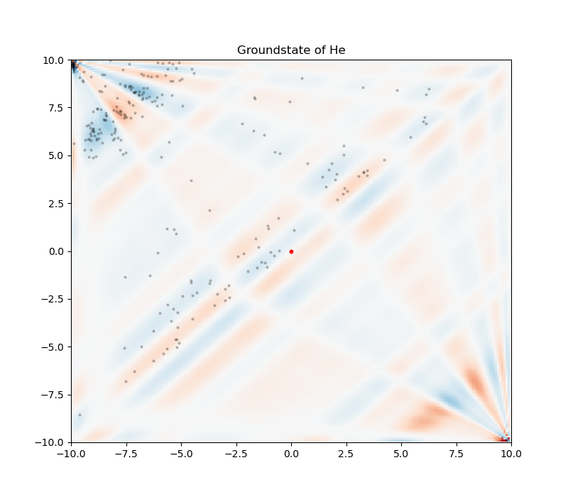
(a) Epoch: 1

(b) Epoch: 10000

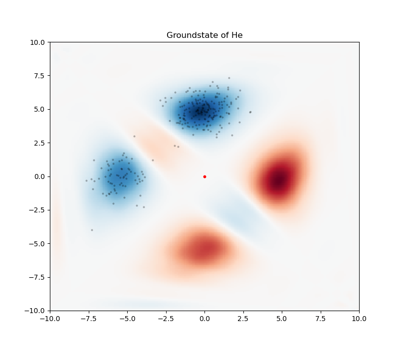
(c) Epoch: 20000

(d) Epoch: 30000

(e) Epoch: 40000

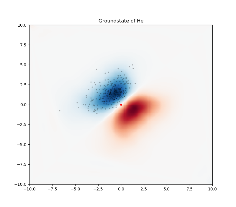
(f) Epoch: 50000

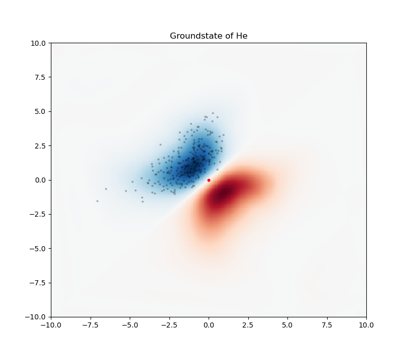
(g) Epoch: 60000

Figure 12: Training progression of Waveflow. The black dots are samples drawn from the Waveflow Ansatz. Note that the samples are only on one side, as we only train the model on that fundamental domain. We can see that 1) the topology of Waveflow can indeed adapt, as there are many more nodes at the beginning of training than there are at the end, and 2) The results look very close to the ground truth result obtained from QMsolve.

References

- Barrett et al. (2022) Barrett, T. D., Malyshev, A., and Lvovsky, A. Autoregressive neural-network wavefunctions for ab initio quantum chemistry. Nature Machine Intelligence, 4(4):351–358, 2022.
- Brown et al. (2020) Brown, T., Mann, B., Ryder, N., Subbiah, M., Kaplan, J. D., Dhariwal, P., Neelakantan, A., Shyam, P., Sastry, G., Askell, A., et al. Language models are few-shot learners. Advances in neural information processing systems, 33:1877–1901, 2020.
- Carleo & Troyer (2017) Carleo, G. and Troyer, M. Solving the quantum many-body problem with artificial neural networks. Science, 355(6325):602–606, 2017.
- Ceperley (1991) Ceperley, D. M. Fermion nodes. Journal of statistical physics, 63(5):1237–1267, 1991.
- Choo et al. (2020) Choo, K., Mezzacapo, A., and Carleo, G. Fermionic neural-network states for ab-initio electronic structure. Nature communications, 11(1):1–7, 2020.
- Chowdhery et al. (2022) Chowdhery, A., Narang, S., Devlin, J., Bosma, M., Mishra, G., Roberts, A., Barham, P., Chung, H. W., Sutton, C., Gehrmann, S., et al. Palm: Scaling language modeling with pathways. arXiv preprint arXiv:2204.02311, 2022.
- Cornish et al. (2020) Cornish, R., Caterini, A., Deligiannidis, G., and Doucet, A. Relaxing bijectivity constraints with continuously indexed normalising flows. In International conference on machine learning, pp. 2133–2143. PMLR, 2020.
- Curry & Schoenberg (1988) Curry, H. B. and Schoenberg, I. J. On pólya frequency functions iv: the fundamental spline functions and their limits. In IJ Schoenberg Selected Papers, pp. 347–383. Springer, 1988.
- Dinh et al. (2014) Dinh, L., Krueger, D., and Bengio, Y. Nice: Non-linear independent components estimation. arXiv preprint arXiv:1410.8516, 2014.
- Dinh et al. (2016) Dinh, L., Sohl-Dickstein, J., and Bengio, S. Density estimation using real nvp. arXiv preprint arXiv:1605.08803, 2016.
- Durkan et al. (2019) Durkan, C., Bekasov, A., Murray, I., and Papamakarios, G. Neural spline flows. Advances in neural information processing systems, 32, 2019.
- Durkan et al. (2019) Durkan, C., Bekasov, A., Murray, I., and Papamakarios, G. Neural Spline Flows. arXiv e-prints, art. arXiv:1906.04032, June 2019.
- Germain et al. (2015) Germain, M., Gregor, K., Murray, I., and Larochelle, H. Made: Masked autoencoder for distribution estimation. In International conference on machine learning, pp. 881–889. PMLR, 2015.
- Guimaraes et al. (2017) Guimaraes, G. L., Sanchez-Lengeling, B., Outeiral, C., Farias, P. L. C., and Aspuru-Guzik, A. Objective-reinforced generative adversarial networks (organ) for sequence generation models. arXiv preprint arXiv:1705.10843, 2017.
- Hammond et al. (1994) Hammond, B., Lester, W., and Reynolds, P. Monte Carlo Methods in Ab Initio Quantum Chemistry. Lecture and Course Notes In Chemistry Series. World Scientific, 1994. ISBN 9789810203214. URL https://books.google.com/books?id=aydqDQAAQBAJ.
- Hermann et al. (2020) Hermann, J., Schätzle, Z., and Noé, F. Deep-neural-network solution of the electronic schrödinger equation. Nature Chemistry, 12(10):891–897, 2020.
- Hermann et al. (2022) Hermann, J., Spencer, J., Choo, K., Mezzacapo, A., Foulkes, W., Pfau, D., Carleo, G., and Noé, F. Ab-initio quantum chemistry with neural-network wavefunctions. arXiv preprint arXiv:2208.12590, 2022.
- Ho et al. (2019) Ho, J., Chen, X., Srinivas, A., Duan, Y., and Abbeel, P. Flow++: Improving flow-based generative models with variational dequantization and architecture design. In International Conference on Machine Learning, pp. 2722–2730. PMLR, 2019.
- Hoffmann et al. (2022) Hoffmann, J., Borgeaud, S., Mensch, A., Buchatskaya, E., Cai, T., Rutherford, E., Casas, D. d. L., Hendricks, L. A., Welbl, J., Clark, A., et al. Training compute-optimal large language models. arXiv preprint arXiv:2203.15556, 2022.
- Huang et al. (2018) Huang, C.-W., Krueger, D., Lacoste, A., and Courville, A. Neural autoregressive flows. In International Conference on Machine Learning, pp. 2078–2087. PMLR, 2018.
- Jing et al. (2022) Jing, B., Corso, G., Chang, J., Barzilay, R., and Jaakkola, T. Torsional diffusion for molecular conformer generation. arXiv preprint arXiv:2206.01729, 2022.
- Jolie et al. (2019) Jolie, W., Murray, C., Weiß, P. S., Hall, J., Portner, F., Atodiresei, N., Krasheninnikov, A. V., Busse, C., Komsa, H.-P., Rosch, A., et al. Tomonaga-luttinger liquid in a box: electrons confined within mos 2 mirror-twin boundaries. Physical Review X, 9(1):011055, 2019.
- Kingma & Ba (2014) Kingma, D. P. and Ba, J. Adam: A method for stochastic optimization. arXiv preprint arXiv:1412.6980, 2014.
- Kingma & Dhariwal (2018) Kingma, D. P. and Dhariwal, P. Glow: Generative flow with invertible 1x1 convolutions. Advances in neural information processing systems, 31, 2018.
- Kirkpatrick et al. (2021) Kirkpatrick, J., McMorrow, B., Turban, D. H., Gaunt, A. L., Spencer, J. S., Matthews, A. G., Obika, A., Thiry, L., Fortunato, M., Pfau, D., et al. Pushing the frontiers of density functionals by solving the fractional electron problem. Science, 374(6573):1385–1389, 2021.
- Klimyk et al. (2007) Klimyk, A., Patera, J., et al. Antisymmetric orbit functions. SIGMA. Symmetry, Integrability and Geometry: Methods and Applications, 3:023, 2007.
- Köhler et al. (2021) Köhler, J., Krämer, A., and Noé, F. Smooth normalizing flows. Advances in Neural Information Processing Systems, 34:2796–2809, 2021.
- Kohn & Sham (1965) Kohn, W. and Sham, L. J. Self-consistent equations including exchange and correlation effects. Phys. Rev., 140:A1133–A1138, Nov 1965. doi: 10.1103/PhysRev.140.A1133. URL https://link.aps.org/doi/10.1103/PhysRev.140.A1133.
- Liu et al. (2019) Liu, X., Nassar, H., and PodgÓrski, K. Splinets – efficient orthonormalization of the b-splines, 2019. URL https://arxiv.org/abs/1910.07341.
- Löwdin (1956) Löwdin, P.-O. Quantum theory of cohesive properties of solids. Advances in Physics, 5(17):1–171, 1956. doi: 10.1080/00018735600101155.
- Luo & Clark (2019) Luo, D. and Clark, B. K. Backflow transformations via neural networks for quantum many-body wave functions. Physical review letters, 122(22):226401, 2019.
- Mann (2010) Mann, R. An Introduction to Particle Physics and the Standard Model. CRC Press, 2010. doi: https://doi.org/10.1201/9781420083002.
- Martens & Grosse (2015) Martens, J. and Grosse, R. Optimizing neural networks with kronecker-factored approximate curvature. In International conference on machine learning, pp. 2408–2417. PMLR, 2015.
- Maziarka et al. (2020) Maziarka, Ł., Pocha, A., Kaczmarczyk, J., Rataj, K., Danel, T., and Warchoł, M. Mol-cyclegan: a generative model for molecular optimization. Journal of Cheminformatics, 12(1):1–18, 2020.
- Nightingale & Umrigar (1998) Nightingale, M. P. and Umrigar, C. J. Quantum Monte Carlo methods in physics and chemistry. Springer Science & Business Media, 1998.
- Noé et al. (2019) Noé, F., Olsson, S., Köhler, J., and Wu, H. Boltzmann generators: Sampling equilibrium states of many-body systems with deep learning. Science, 365(6457):eaaw1147, 2019.
- Orús (2014) Orús, R. A practical introduction to tensor networks: Matrix product states and projected entangled pair states. Annals of Physics, 349:117–158, 2014. ISSN 0003-4916. doi: https://doi.org/10.1016/j.aop.2014.06.013. URL https://www.sciencedirect.com/science/article/pii/S0003491614001596.
- Papamakarios et al. (2017) Papamakarios, G., Pavlakou, T., and Murray, I. Masked autoregressive flow for density estimation. Advances in neural information processing systems, 30, 2017.
- Pfau et al. (2020) Pfau, D., Spencer, J. S., Matthews, A. G., and Foulkes, W. M. C. Ab initio solution of the many-electron schrödinger equation with deep neural networks. Physical Review Research, 2(3):033429, 2020.
- Piegl & Tiller (1996) Piegl, L. and Tiller, W. The NURBS book. Springer Science & Business Media, 1996.
- Rafael de la Fuente (2022) Rafael de la Fuente, m. Qmsolve. https://github.com/quantum-visualizations/qmsolve, 2022.
- Ramesh et al. (2022) Ramesh, A., Dhariwal, P., Nichol, A., Chu, C., and Chen, M. Hierarchical text-conditional image generation with clip latents. arXiv preprint arXiv:2204.06125, 2022.
- Ramsay (1988) Ramsay, J. O. Monotone regression splines in action. Statistical science, pp. 425–441, 1988.
- Rezende & Mohamed (2015) Rezende, D. and Mohamed, S. Variational inference with normalizing flows. In International conference on machine learning, pp. 1530–1538. PMLR, 2015.
- Saharia et al. (2022) Saharia, C., Chan, W., Saxena, S., Li, L., Whang, J., Denton, E., Ghasemipour, S. K. S., Ayan, B. K., Mahdavi, S. S., Lopes, R. G., et al. Photorealistic text-to-image diffusion models with deep language understanding. arXiv preprint arXiv:2205.11487, 2022.
- Schwartz (2013) Schwartz, M. D. Quantum Field Theory and the Standard Model. Cambridge University Press, 2013. doi: 10.1017/9781139540940.
- Sharir et al. (2020) Sharir, O., Levine, Y., Wies, N., Carleo, G., and Shashua, A. Deep autoregressive models for the efficient variational simulation of many-body quantum systems. Physical review letters, 124(2):020503, 2020.
- Sholl & Steckel (2011) Sholl, D. and Steckel, J. Density Functional Theory: A Practical Introduction. Wiley, 2011. ISBN 9781118211045. URL https://books.google.com/books?id=_f994dmAdv0C.
- Szabo et al. (1982) Szabo, A., Szabó, A., and Ostlund, N. Modern Quantum Chemistry: Introduction to Advanced Electronic Structure Theory. Macmillan, 1982. ISBN 9780029497104. URL https://books.google.com/books?id=1ky8QgAACAAJ.
- Toulouse et al. (2015) Toulouse, J., Assaraf, R., and Umrigar, C. J. Introduction to the variational and diffusion Monte Carlo methods. arXiv e-prints, art. arXiv:1508.02989, August 2015.
- White (1992) White, S. R. Density matrix formulation for quantum renormalization groups. Phys. Rev. Lett., 69:2863–2866, Nov 1992. doi: 10.1103/PhysRevLett.69.2863. URL https://link.aps.org/doi/10.1103/PhysRevLett.69.2863.
- Xie et al. (2021) Xie, H., Zhang, L., and Wang, L. Ab-initio study of interacting fermions at finite temperature with neural canonical transformation. arXiv preprint arXiv:2105.08644, 2021.
- Xu et al. (2021) Xu, M., Luo, S., Bengio, Y., Peng, J., and Tang, J. Learning neural generative dynamics for molecular conformation generation. arXiv preprint arXiv:2102.10240, 2021.
- Xu et al. (2022) Xu, M., Yu, L., Song, Y., Shi, C., Ermon, S., and Tang, J. Geodiff: A geometric diffusion model for molecular conformation generation. arXiv preprint arXiv:2203.02923, 2022.
- Yu et al. (2022) Yu, J., Xu, Y., Koh, J. Y., Luong, T., Baid, G., Wang, Z., Vasudevan, V., Ku, A., Yang, Y., Ayan, B. K., et al. Scaling autoregressive models for content-rich text-to-image generation. arXiv preprint arXiv:2206.10789, 2022.
- Zhao et al. (2021) Zhao, T., De, S., Chen, B., Stokes, J., and Veerapaneni, S. Overcoming barriers to scalability in variational quantum monte carlo. In Proceedings of the International Conference for High Performance Computing, Networking, Storage and Analysis, pp. 1–13, 2021.