Numerical analysis of a time discretized method for nonlinear filtering problem with Lévy process observations

Abstract

In this paper, we consider a nonlinear filtering model with observations driven by correlated Wiener processes and point processes. We first derive a Zakai equation whose solution is an unnormalized probability density function of the filter solution. Then we apply a splitting-up technique to decompose the Zakai equation into three stochastic differential equations, based on which we construct a splitting-up approximate solution and prove its half-order convergence. Furthermore, we apply a finite difference method to construct a time semi-discrete approximate solution to the splitting-up system and prove its half-order convergence to the exact solution of the Zakai equation. Finally, we present some numerical experiments to demonstrate the theoretical analysis.

1 Introduction

The aim of a nonlinear filtering problem is to seek the conditional expectation, which is the best estimate of the unobserved state of a stochastic dynamical system given its partial observation. The observation is usually described as a nonlinear stochastic differential equation driven by a noise process. In many applications, such as biology dawson2015 , physics MiSK1979 , target tracking yang2012 and weather forecast AnML2004 , the noise can be characterized by a standard Wiener process. However, in some applications, such as the number of customers arriving at a supermarket DaSu2013 and the number of births in a given period of time Young1998 , the noise is governed by a point process. In some other applications such as the credit risk models FrSch2012 ; FRXL2013 , mathematical finance bremaud1972 ; FrRS2009 and insurance AgLa2007 ; CeCl2015 , the noise can be described by a mixture of a Wiener process and a point process, which is usually called Lévy process.

There have been a few theoretical and numerical studies on nonlinear filtering problems driven by Lévy processes. Qiao and Duan QiDu2015 studied a nonlinear filtering model where both the state and observation involve point processes. They simultaneously derived the Zakai equations and Kushner-Stratonovich equations and proved their well-posedness. Fernando and Hausenblas FeHa2018 investigated a nonlinear filter model with correlated point processes for the state and observation. They provided sufficient conditions for the well-posedness of the corresponding Zakai equation. Frey etc. FRXL2013 used the PDF filter method to approximate a nonlinear filter model driven by point processes and independent Wiener processes. The PDF filter method is designed to directly approach the conditional density function, which satisfies a stochastic partial differential equation, namely Zakai equation zakai1969 . In FRXL2013 the authors applied a spectral Galerkin method to set up a spatial semi-discrete equation and proved that its solution converges to the exact solution of the Zakai equation. However, they did not provide the convergence order. They also used the Euler-Maruyama scheme and a splitting-up method, to discretize temporal variables.

In this paper, we use the splitting-up method to investigate the numerical approximation of a nonlinear filtering model where the observation is driven by the mixture of point processes and correlated Wiener processes. The splitting-up method BaGrRa ; FlFr1991 ; GyIs2003 is a well-known strategy for solving Zakai equations. It decomposes the Zakai equation into a system consisting of deterministic PDEs and stochastic differential equations (SDEs) Ito1996 ; AnML2004 ; BaoCao2014 ; BaGrRa ; FlFr1991 . Our contribution in this paper is twofold. First, we decompose the Zakai equation into three equations: an SDE driven by the Wiener process, a second order parabolic equation satisfying the uniform elliptic condition, and an SDE driven by a point process. Through the solution operators of the three equations and their a priori estimates, we construct a splitting-up approximation and prove that it converges to the Zakai solution with first order accuracy. We note that in some references FPLe1991 ; LeFr1992 ; GyIs2003 concerning the nonlinear filtering models with correlated noises, the decomposed second-order parabolic equation is possibly degenerate, which may cause difficulty for numerical implementations. Our second contribution is the derivation of the half-order convergence of the time semi-discrete approximation. To the best of our knowledge, this is the first time a convergence order of a numerical method for nonlinear filtering problems with jump processes has been provided.

This paper is organized as follows. In section 2, we introduce a nonlinear filtering model with the mixed noise of point process and correlated Wiener process and then derive the corresponding Zakai equation. In section 3, we apply a splitting-up method to construct a splitting-up approximate solution to the Zakai equation and establish a priori estimates for the splitting-up solution and show that the convergence is of half order. In section 4, we use finite difference methods to construct a time semi-discrete approximation and prove that the semi-discrete solution converges to the exact solution with half order. Finally in section 5, we present some numerical experiments to illustrate our theoretical analysis.

2 A nonlinear filtering model with jump observations and its Zakai equation

In this section, we first introduce a nonlinear filtering model whose observations are driven by Lévy processes. Then we derive the corresponding Zakai equation which characterizes the development of the density function of the filtering solution process. Finally, we investigate the regularity of the solution of the Zakai equation.

2.1 A nonlinear filtering model

In this subsection, we introduce a nonlinear filtering model with noises simultaneously driven by a point and correlated Wiener processes and then discuss some basic assumptions.

Let $(\Omega,{\cal{F}},P)$ be a given probability space. Consider a nonlinear filtering model whose state (or signal) process $X_{t}$ and two observation processes $Y_{t}$ and $Z_{t}$ are given by

$$X_{t}=X_{0}+\int_{0}^{t}g(X_{s},Y_{s})ds+\int_{0}^{t}\sigma(X_{s})dw_{s},\quad 0\leq t\leq T,$$ (1)

$$Y_{t}=Y_{0}+\int_{0}^{t}h(X_{s})ds+\int_{0}^{t}b(Y_{s})dw_{s}+\int_{0}^{t}\tilde{b}(Y_{s})dv_{s},\quad 0\leq t\leq T,$$ (2)

$$Z_{t}~{}\text{is a doubly stochastic Poisson process with density function}~{}\lambda(X_{t}),$$ (3)

where $w_{t}\in\mathbb{R}^{m_{1}}$ and $v_{t}\in\mathbb{R}^{m_{2}}$ are two standard independent Winner processes, $Z_{t}$ is a doubly stochastic Poisson process with a continuous density function $\lambda:\mathbb{R}^{d}\to[\varpi_{1},\varpi_{2}]\subset\mathbb{R}_{+}$ such that $Z_{t}-\int_{0}^{t}\lambda(X_{s})ds$ is a martingale. The corresponding jump times for $Z_{t}$ are random variables denoted by $\tau_{1}<\tau_{2}<\cdots<\tau_{n_{0}}$, where $n_{0}$ is an integer-valued random variable.

The objective of the nonlinear filtering problem is to seek an optimal estimation of $X_{t}$ based on observations $Y_{t}$ and $Z_{t}$, which is characterized by the conditional expectation $E[X_{t}|Y_{t},Z_{t}]$. Now, we describe in detail the assumptions used in this work.

• $E|X_{0}|^{2}+E|Y_{0}|^{2}<\infty$.

• $g:\mathbb{R}^{d}\times\mathbb{R}^{q}\to\mathbb{R}^{d}$ and $h:\mathbb{R}^{d}\to\mathbb{R}^{q}$ are bounded, continuous and square integrable, $\sigma:\mathbb{R}^{d}\to\mathbb{R}^{d\times m_{1}}$ is in $C^{2}$ with bounded first and second order derivatives, and $b$, $\tilde{b}$ are in $C^{1}$ with bounded first order derivatives.

Define two families of symmetric non-negative matrix

$$A(x)=(a_{i,j}(x))_{d\times d}=\frac{1}{2}\sigma(x)\sigma^{T}(x),\quad D(y)=b(y)b(y)^{T}+\tilde{b}(y)\tilde{b}(y)^{T}.$$

• There exist two constants $0<\alpha_{1}<\alpha_{2}$ such that for any $x\in\mathbb{R}^{d}$, $y\in\mathbb{R}^{q}$ and $u\in\mathbb{R}^{q}$, there hold

  $$\alpha_{1}\|u\|^{2}\leq u^{T}A(x)u\leq\alpha_{2}\|u\|^{2},$$

  $$\alpha_{1}\|u\|^{2}\leq u^{T}D(y)u\leq\alpha_{2}\|u\|^{2}.$$

Define two Sobolev spaces $H=L^{2}(\mathbb{R}^{d})$ with norm $\|\cdot\|$ and $V=H^{1}_{0}(\mathbb{R}^{d})$ with norm $\|\cdot\|_{1}$. By $V^{\prime}$, we denote the dual space of $V$. Obviously, for any $\forall\phi\in{V}\subset H\subset V^{\prime}$ there holds

$$\|\phi\|_{V^{\prime}}\leq\|\phi\|\leq\|\phi\|_{1}.$$ (4)

Define a filtration associated with the observations by

$$\mathcal{F}_{t}=\sigma(Y_{s},Z_{s},~{}0\leq s\leq t),\quad t\in[0,T],$$

which is right continuous and complete. By $\mathbb{L}^{2}(0,T\mathchar 24635\relax\;V)$ we denote a Hilbert space consisting of $\mathcal{F}_{t}$ progressively measurable $V$-valued stochastic process $z(t)$ with $E\int_{0}^{T}\|z(t)\|_{1}^{2}dt<\infty$.

2.2 Zakai equation and its regularity

The main task of this subsection is to derive the Zakai equation of the nonlinear filtering model (1)-(3) and study the regularity of its solution.

Assume that $X_{t}$ is the solution process of (1). For any $\phi\in C_{0}^{\infty}(\mathbb{R}^{d})$, define $\pi_{t}(\phi)$ as the conditional expectation of $\phi(X_{t})$ given $\mathcal{F}_{t}$, i.e.,

$$\pi_{t}(\phi):=E\big{(}\phi(X_{t})|\mathcal{F}_{t}\big{)}.$$ (5)

For any $t\in[0,T]$, define

$$\eta_{t}={} \prod\limits_{\tau_{m}\leq t}\lambda(X_{\tau_{m}-})\cdot\exp\left(\int^{t}_{0}h^{T}(X_{s})D^{-1}(b(Y_{s})dw_{s}+\tilde{b}(Y_{s})dv_{s})\right.$$ (6)

$$\left.+\frac{1}{2}\int^{t}_{0}h^{T}(X_{s})D^{-1}h(X_{s})ds-\int_{0}^{t}(\lambda(X_{s})-1)ds\right).$$

According to Novikov Criterion (Protter2005, , Theorem 41), $\eta_{t}$ is a nonnegative martingale if H1-H3 hold. Define a new probability measure $\tilde{P}$ by virtue of the Radon-Nikodym derivative $\frac{d\tilde{P}}{dP}=\eta_{t}^{-1}$. The Girsanov theorem BaCr2009 implies that $\bar{Y}_{t}=\int_{0}^{t}D(Y_{s})^{-1/2}dY_{s}$ is a standard Wiener process and $Z_{t}$ is a Poisson process with intensity equal to $1$ under the probability measure $\tilde{P}$. Furthermore, in the probability space $(\Omega,\mathcal{F},\tilde{P})$ the three stochastic processes $X_{t}$, $Y_{t}$ and $Z_{t}$ are independent of each other, and the compensated Poisson process $N_{t}:=Z_{t}-t$ is a martingale.

Define a stochastic process

$$\tilde{Y}_{t}=\int_{0}^{t}[I-b^{T}D^{-1}b]^{-1/2}(d\tilde{w}_{t}-b^{T}D^{-1}dY_{t}),$$

where $\tilde{w}_{t}=w_{t}+\int_{0}^{t}b^{T}(Y_{s})D^{-1}(Y_{s})h(X_{s})ds$ is a standard Wiener process under $\tilde{P}$. From Pard1981 , we have

Lemma 1.

Assume H1-H3. Then $\tilde{Y}_{t}$ is a standard Wiener process independent of $Y_{t}$ under $\tilde{P}$ and equation (1) is equivalent to

$$X_{t}=X_{0}\!+\!\!\int_{0}^{t}\!\![g(X_{s})\!-\!B_{1}(X_{s},Y_{s})h(X_{s})]ds\!+\!\!\int_{0}^{t}\!\!B_{1}(X_{s},Y_{s})dY_{s}\!+\!\!\int_{0}^{t}\!\!B_{2}(X_{s},Y_{s})d\tilde{Y}_{s},$$

where $B_{1}(x,y)=\sigma(x)b^{T}(y)D^{-1}(y)$ and $B_{2}(x,y)=\sigma(x)(I-b^{T}(y)D^{-1}(y)b(y))^{1/2}$.

Denote by $\tilde{E}$ the expectation under the probability measure $\tilde{P}$. The next proposition plays an important role in the forthcoming analysis.

Proposition 2.

(BaCr2009, , Proposition 3.15) Assume that H1-H3 hold and let $U$ be an $\mathcal{F}_{t}$-measurable and integrable random variable. Then we have

$$\tilde{E}[U|\mathcal{F}_{t}]=\tilde{E}[U|\mathcal{F}_{T}].$$ (7)

By the Kallianpur-Striebel formula (BaCr2009, , Proposition 3.16), we have

$$\pi_{t}(\phi)=\frac{\tilde{E}(\phi(X_{t})\eta_{t}|\mathcal{F}_{t})}{\tilde{E}(\eta_{t}|\mathcal{F}_{t})}=\frac{(p(t),\phi)}{(p(t),1)},$$ (8)

where $p(t)$ is the unnormalized conditional density function of $\tilde{E}(X_{t}|\mathcal{F}_{t})$.

Theorem 3.

Assume that H1-H3 hold and let $\rho_{t}(\phi)=(p(t),\phi)$. Then $\rho_{t}$ satisfies a functional equation: for $\forall\phi\in C_{0}^{\infty}(\mathbb{R}^{d})$ and $0\leq t\leq T$,

$$\rho_{t}(\phi)=\rho_{0}(\phi)+\int_{0}^{t}\rho_{s}(\mathcal{L}\phi)ds+\int_{0}^{t}\rho_{s}(\mathcal{B}\phi)dY_{s}+\int_{0}^{t}\rho_{s-}\big{(}\phi(\lambda-1)\big{)}d(Z_{s}-s),\quad\tilde{P}-a.s.,$$ (9)

where

$$\mathcal{L}\phi = \sum\limits_{i,j=1}^{d}a_{i,j}(x)\frac{\partial^{2}\phi}{\partial x_{i}\partial x_{j}}+\sum\limits_{i=1}^{d}g_{i}(x)\frac{\partial\phi}{\partial x_{i}},$$

$$\mathcal{B}\phi = \phi h^{T}D^{-1}+\sum\limits_{i=1}^{d}\frac{\partial\phi}{\partial x_{i}}b_{1,i},$$

and $b_{1,i}$ denotes the $i$-th row of matrix $B_{1}(x,y)$.

Proof: We approximate $\eta_{t}$ with $\eta_{t}^{\varepsilon}=\frac{\eta_{t}}{1+\varepsilon\eta_{t}}$. By Itô formula

$$d\eta_{t}=\eta_{t-}\big{[}h(X_{t})^{T}D^{-1}dY_{t}+(\lambda(X_{t-})-1)d(Z_{t}-t)\big{]}.$$ (10)

Using Itô’s formula for the jump process, we have

$$\eta_{t}^{\varepsilon}={} \eta_{0}^{\varepsilon}+\int_{0}^{t}\frac{\eta_{s}}{(1+\varepsilon\eta_{s})^{2}}h(X_{s})^{T}D^{-1}dY_{s}-\int_{0}^{t}\frac{\varepsilon\eta_{t}^{2}}{(1+\varepsilon\eta_{t})^{3}}h(X_{s})^{T}D^{-1}h(X_{s})ds$$ (11)

$$-\int_{0}^{t}\frac{\eta_{s}}{(1+\varepsilon\eta_{s})^{2}}(\lambda(X_{s})-1)ds+\sum_{\tau_{m}\leq t}\Delta\frac{\eta_{\tau_{m}}}{1+\varepsilon\eta_{\tau_{m}}}.$$

Let $X_{t}$ satisfy (1) and for any $\phi\in C_{0}^{\infty}(\mathbb{R}^{d})$

$$d\phi(X_{t})={} \mathcal{L}\phi dt-\sum\limits_{i=1}^{d}(B_{1}h)^{i}\frac{\partial\phi}{\partial x_{i}}dt+\nabla\phi^{T}B_{1}dY_{t}+\nabla\phi^{T}B_{2}d\tilde{Y}_{t}.$$ (12)

Applying the product rule for semi-martingales to (10) and (12), we obtain

$$\eta_{t}^{\varepsilon}\phi(X_{t})$$ (13)

$$={} \eta_{0}^{\varepsilon}\phi(X_{0})+\int_{0}^{t}\eta_{s}^{\varepsilon}\mathcal{L}\phi(X_{s})ds-\int_{0}^{t}\frac{\varepsilon\eta_{s}^{2}}{(1+\varepsilon\eta_{s})^{2}}\nabla\phi^{T}B_{1}hds+\int_{0}^{t}\eta_{s}^{\varepsilon}\nabla\phi^{T}B_{1}dY_{s}$$

$$+\int_{0}^{t}\eta_{s}^{\varepsilon}\nabla\phi^{T}B_{2}d\tilde{Y}_{s}+\int_{0}^{t}\frac{\eta_{s}\phi(X_{s})}{(1+\varepsilon\eta_{s})^{2}}h^{T}D^{-1}dY_{s}-\int_{0}^{t}\frac{\varepsilon\eta_{s}^{2}\phi(X_{s})}{(1+\varepsilon\eta_{s})^{2}}h^{T}D^{-1}hds$$

$$-\int_{0}^{t}\frac{\eta_{s}\phi(X_{s})}{(1+\varepsilon\eta_{s})^{2}}(\lambda(X_{s})-1)ds+\int_{0}^{t}\frac{\eta_{s-}(\lambda(X_{s-})-1)\phi(X_{s-})}{(1+\varepsilon\eta_{s-}\lambda(X_{s-}))(1+\varepsilon\eta_{s-})}dZ_{s}.$$

According to Proposition 2, we only need to compute the conditional expectation based on the filtration $\mathcal{F}_{T}$. Take conditional expectation about $\eta_{t}^{\varepsilon}\phi(X_{t})$ based on the observation $\mathcal{F}_{T}$, then we have

$$\tilde{E}(\eta_{t}^{\varepsilon}\phi(X_{t})\rvert\mathcal{F}_{T})$$ (14)

$$={} \tilde{E}(\eta_{0}^{\varepsilon}\phi(X_{0})\rvert\mathcal{F}_{T})+\tilde{E}\bigg{(}\int_{0}^{t}\eta_{s}^{\varepsilon}\mathcal{L}\phi(X_{s})ds\rvert\mathcal{F}_{T}\bigg{)}$$

$$-\tilde{E}\bigg{(}\int_{0}^{t}\frac{\varepsilon\eta_{s}^{2}}{(1+\varepsilon\eta_{s})^{2}}\nabla\phi^{T}B_{1}hds\rvert\mathcal{F}_{T}\bigg{)}+\tilde{E}\bigg{(}\int_{0}^{t}\eta_{s}^{\varepsilon}\nabla\phi^{T}B_{1}dY_{s}\rvert\mathcal{F}_{T}\bigg{)}$$

$$+\tilde{E}\bigg{(}\int_{0}^{t}\frac{\eta_{s}\phi}{(1+\varepsilon\eta_{s})^{2}}h^{T}D^{-1}dY_{s}\rvert\mathcal{F}_{T}\bigg{)}+\tilde{E}\bigg{(}\int_{0}^{t}\eta_{s}^{\varepsilon}\nabla\phi^{T}B_{2}d\tilde{Y}_{s}\rvert\mathcal{F}_{T}\bigg{)}$$

$$-\tilde{E}\bigg{(}\int_{0}^{t}\frac{\varepsilon\eta_{s}^{2}\phi}{(1+\varepsilon\eta_{s})^{3}}h^{T}D^{-1}hds\rvert\mathcal{F}_{T}\bigg{)}-\tilde{E}\bigg{(}\int_{0}^{t}\frac{\eta_{s}\phi}{(1+\varepsilon\eta_{s})^{2}}(\lambda(X_{s})-1)ds\rvert\mathcal{F}_{T}\bigg{)}$$

$$+\tilde{E}\bigg{(}\int_{0}^{t}\frac{\eta_{s-}(\lambda(X_{s-})-1)\phi(X_{s-})}{(1+\varepsilon\eta_{s-}\lambda(X_{s-}))(1+\varepsilon\eta_{s-})}dZ_{s}\rvert\mathcal{F}_{T}\bigg{)}$$

$$:={} E_{1}+E_{2}-E_{3}+E_{4}+E_{5}+E_{6}-E_{7}-E_{8}+E_{9}.$$

Now, we show that as $\varepsilon\rightarrow 0$, the following limits hold in the sense $\tilde{P}$-a.s.,

$$\tilde{E}(\eta_{t}^{\varepsilon}\rvert\mathcal{F}_{T})\rightarrow\rho_{t}(\phi),\quad E_{1}\rightarrow\rho_{0}(\phi),\quad E_{2}\rightarrow\int_{0}^{t}\rho_{s}(\mathcal{L}\phi)ds,\quad E_{3}\rightarrow 0,$$

$$E_{4}\rightarrow\int_{0}^{t}\rho_{s}(\nabla\phi^{T}c)dY_{s},\quad E_{5}\rightarrow\int_{0}^{t}\rho_{s}(h^{T}D^{-1}\phi)dY_{s},\quad E_{6}\rightarrow 0,\quad E_{7}\rightarrow 0,$$

$$E_{8}\rightarrow\int_{0}^{t}\rho_{s}(\phi(\lambda-1))ds,\quad E_{9}\rightarrow\int_{0}^{t}\rho_{s-}(\phi(\lambda-1))dZ_{s}.$$

From the pointwise convergence of $\eta_{t}^{\varepsilon}$ to $\eta_{t}$ as $\varepsilon\to 0$, it follows that $\lim\limits_{\varepsilon\rightarrow 0}\eta_{t}^{\varepsilon}\phi=\eta_{t}\phi$. In addition,

$$\tilde{E}\|\eta_{t}^{\varepsilon}\phi\|\leq\|\phi\|_{\infty}\tilde{E}(\eta_{t})=\|\phi\|_{\infty}E(\eta_{t}\eta_{t}^{-1})=\|\phi\|_{\infty}<\infty.$$

Due to the dominated convergence theorem (ReDY1999, , page 152), we obtain

$$\lim_{\varepsilon\rightarrow 0}\tilde{E}(\eta_{t}^{\varepsilon}\phi|\mathcal{F}_{T})=\tilde{E}(\eta_{t}\phi|\mathcal{F}_{T})=\rho_{t}(\phi),\quad\tilde{P}-a.s.$$

Similarly, there holds

$$\lim_{\varepsilon\rightarrow 0}E_{1}=\tilde{E}(\eta_{0}\phi(X_{0})|\mathcal{F}_{T})=\rho_{0}(\phi),\quad\tilde{P}-a.s.$$

Now, we consider item $E_{2}$. Notice that for any $\varepsilon>0$, there holds

$$\tilde{E}\bigg{(}\|\int_{0}^{t}\eta_{t}^{\varepsilon}\mathcal{L}\phi ds\|\big{|}\mathcal{F}_{T}\bigg{)}=\tilde{E}\bigg{(}\|\int_{0}^{t}\frac{\varepsilon\eta_{s}}{1+\varepsilon\eta_{s}}\frac{1}{\varepsilon}\mathcal{L}\phi ds\|\big{|}\mathcal{F}_{T}\bigg{)}\leq\frac{1}{\varepsilon}\|\mathcal{L}\phi\|_{\infty}T<\infty.$$

By Fubini’s theorem, we exchange the integral order in $E_{2}$ to obtain

$$\|E_{2}\| =\|\tilde{E}\bigg{(}\int_{0}^{t}\eta_{s}^{\varepsilon}\mathcal{L}\phi ds\rvert\mathcal{F}_{T}\bigg{)}\|=\|\int_{0}^{t}\tilde{E}(\eta_{s}^{\varepsilon}\mathcal{L}\phi|\mathcal{F}_{T})ds\|$$

$$\leq\tilde{E}\bigg{(}\int_{0}^{t}\tilde{E}(\|\eta_{t}^{\varepsilon}\mathcal{L}\phi\|\rvert\mathcal{F}_{T})ds\bigg{)}\leq{}\tilde{E}\bigg{(}\int_{0}^{t}\tilde{E}(\eta_{s}\|\mathcal{L}\phi\|_{\infty}|\mathcal{F}_{T})ds\bigg{)}$$

$$=\|\mathcal{L}\phi\|_{\infty}\int_{0}^{t}\tilde{E}(\eta_{s})ds\leq\|\mathcal{L}\phi\|_{\infty}{\color[rgb]{0,0,1}T}<\infty.$$

By the dominated convergence theorem, we get

$$\lim_{\varepsilon\rightarrow 0}E_{2}=\int_{0}^{t}\tilde{E}(\eta_{s}\mathcal{L}\phi|\mathcal{F}_{T})ds=\int_{0}^{t}\rho_{s}(\mathcal{L}\phi)ds,\quad\tilde{P}-a.s.$$

Next, we study item $E_{3}$. Notice that

$$\tilde{E}\bigg{(}\int_{0}^{t}\|\frac{\varepsilon\eta_{s}^{2}}{(1+\varepsilon\eta_{s})^{2}}\nabla\phi^{T}B_{1}h\|ds\bigg{)}\leq{} \|\nabla\phi\|\tilde{E}\big{(}\int_{0}^{t}\eta_{s}\|B_{1}h\|ds\big{)}$$

$$={} \|\nabla\phi\|\int_{0}^{t}E(\|B_{1}h\|)ds<\infty.$$

This estimate, together with the the pointwise convergence $\lim\limits_{\varepsilon\rightarrow 0}\frac{\varepsilon\eta_{t}^{2}}{(1+\varepsilon\eta_{t})^{2}}\nabla\phi^{T}B_{1}h=0$ and the dominated convergence theorem implies

$$\lim\limits_{\varepsilon\rightarrow 0}E_{3}=0,\quad\tilde{P}-a.s.$$

In a similar way, we obtain $\lim\limits_{\varepsilon\rightarrow 0}E_{i}=0$, $\tilde{P}-a.s.$ for $i=6,7$.

By isometry formula, we have that for any $\varepsilon>0$

$$\tilde{E}\left((\int_{0}^{t}\eta_{s}^{\varepsilon}\nabla\phi^{T}B_{1}dY_{s})^{2}\right)$$

$$={} \tilde{E}\bigg{(}\int_{0}^{t}\big{(}\frac{\eta_{s}}{1+\varepsilon\eta_{s}}\big{)}^{2}\nabla\phi^{T}B_{1}DB_{1}^{T}\nabla\phi ds\bigg{)}$$

$$={} \frac{1}{\varepsilon}\tilde{E}\bigg{(}\int_{0}^{t}\frac{\varepsilon\eta_{s}}{(1+\varepsilon\eta_{s})^{2}}\eta_{s}\nabla\phi^{T}B_{1}DB_{1}^{T}\nabla\phi ds\bigg{)}$$

$$\leq{} \frac{\|\nabla\phi\|^{2}}{\varepsilon}\tilde{E}\big{(}\int_{0}^{t}\eta_{s}\|B_{1}DB_{1}^{T}\|ds\big{)}={}\frac{\|\nabla\phi\|^{2}}{\varepsilon}\int_{0}^{t}E(\|B_{1}DB_{1}^{T}\|)ds<\infty.$$

According to (BaCr2009, , Lemma 3.21), we can change the order between conditional expectation and stochastic integral to obtain

$$E_{4}=\int_{0}^{t}\tilde{E}\big{(}\frac{\eta_{s}}{1+\varepsilon\eta_{s}}\nabla\phi^{T}B_{1}|\mathcal{F}_{T}\big{)}dY_{s}.$$ (15)

Using Jensen’s inequality and Fubini’s Theorem, for any $\varepsilon>0$, we have

$$\tilde{E}(E_{4}^{2})$$

$$= \tilde{E}\left\{\int_{0}^{t}\big{[}\tilde{E}(\frac{\eta_{s}}{1+\varepsilon\eta_{s}}\nabla\phi^{T}B_{1}|\mathcal{F}_{T})\big{]}D\big{[}\tilde{E}(\frac{\eta_{s}}{1+\varepsilon\eta_{s}}\nabla\phi^{T}B_{1}|\mathcal{F}_{T})\big{]}^{T}ds\right\}$$

$$\leq \tilde{E}\left\{\int_{0}^{t}\tilde{E}\big{[}(\frac{\eta_{s}}{1+\varepsilon\eta_{s}}\nabla\phi^{T}B_{1})D(\frac{\eta_{s}}{1+\varepsilon\eta_{s}}\nabla\phi^{T}B_{1})^{T}|\mathcal{F}_{T}\big{]}ds\right\}$$

$$\leq \tilde{E}\left\{\int_{0}^{t}\tilde{E}\big{[}\|\nabla\phi\|^{2}\|B_{1}DB_{1}^{T}\|\frac{1}{\varepsilon}\frac{\varepsilon\eta_{s}}{1+\varepsilon\eta_{s}}\eta_{s}|\mathcal{F}_{T}\big{]}ds\right\}$$

$$\leq \frac{\|\nabla\phi\|^{2}}{\varepsilon}\tilde{E}\bigg{(}\int_{0}^{t}\tilde{E}(\eta_{s}\|B_{1}DB_{1}^{T}\|)ds\bigg{)}=\frac{\|\nabla\phi\|^{2}}{\varepsilon}\int_{0}^{t}\tilde{E}(\eta_{s}\|B_{1}DB_{1}^{T}\|)ds$$

$$= \frac{\|\nabla\phi\|^{2}}{\varepsilon}\int_{0}^{t}E(\|B_{1}DB_{1}^{T}\|)ds<\infty.$$

This implies that $E_{4}$ is a martingale, c.f. (ShSE2004, , Theorem 4.3.1) and then the process $\int_{0}^{t}\rho_{s}(\nabla\phi^{T}B_{1})dY_{s}$ is a local martingale. Thus, the following difference is a local martingale

$$\int_{0}^{t}\rho_{s}(\nabla\phi^{T}B_{1})dY_{s}-E_{4}=\int_{0}^{t}\tilde{E}\big{(}\frac{\varepsilon(\eta_{s})^{2}}{1+\varepsilon\eta_{s}}\nabla\phi^{T}B_{1}|\mathcal{F}_{T}\big{)}dY_{s}.$$ (16)

Set $\xi_{s}^{\varepsilon}=\frac{\varepsilon(\eta_{s}^{2})}{1+\varepsilon\eta_{s}}\nabla\phi^{T}B_{1}$, then $\lim\limits_{\varepsilon\rightarrow 0}\xi_{s}^{\varepsilon}=0$, $\tilde{P}-a.s.$ Obviously, for any $\phi\in V$ we have

$$\|\xi_{s}^{\varepsilon}\|\leq\|\nabla\phi\|\|B_{1}\|\eta_{s}.$$

Due to the dominated convergence theorem, we obtain

$$\lim\limits_{\varepsilon\rightarrow 0}\tilde{E}(\xi_{s}^{\varepsilon}|\mathcal{F}_{T})=\tilde{E}(\lim\limits_{\varepsilon\rightarrow 0}\xi_{s}^{\varepsilon}|\mathcal{F}_{T})=0,\tilde{P}-a.s.$$

Furthermore,

$$\|\tilde{E}(\xi_{s}^{\varepsilon}|\mathcal{F}_{T})\|\leq\tilde{E}(\|\xi_{s}^{\varepsilon}\||\mathcal{F}_{T})\leq\|\nabla\phi\|\|B_{1}\|\tilde{E}{(\eta_{s}|\mathcal{F}_{T})}\leq\|\nabla\phi\|\|B_{1}\|.$$ (17)

Applying the stochastic dominated convergence theorem (Protter2005, , Theorem 32), we have

$$\lim\limits_{\varepsilon\rightarrow 0}\int_{0}^{t}\tilde{E}(\xi_{s}^{\varepsilon}|\mathcal{F}_{T})dY_{s}=\int_{0}^{t}\lim\limits_{\varepsilon\rightarrow 0}\tilde{E}(\xi_{s}^{\varepsilon}|\mathcal{F}_{T})dY_{s}=0,\quad\tilde{P}-a.s.$$

Hence, we obtain

$$\lim\limits_{\varepsilon\rightarrow 0}E_{4}=\int_{0}^{t}\rho_{s}(\nabla\phi B_{1})dY_{s},\quad\tilde{P}-a.s.$$

Similarly, we can prove that

$$\lim\limits_{\varepsilon\rightarrow 0}E_{5}=\int_{0}^{t}\rho_{s}(\phi h^{T}D^{-1})dY_{s},\quad\lim\limits_{\varepsilon\rightarrow 0}E_{8}=\int_{0}^{t}\rho_{s}(\phi(\lambda-1))ds,\quad\tilde{P}-a.s.\\$$

Finally, we investigate the term $E_{9}$. Let

$$G_{s}^{\varepsilon}:=\frac{\eta_{s-}(\lambda(X_{s-})-1)\phi(X_{s-})}{(1+\varepsilon\eta_{s-}\lambda(X_{s-}))(1+\varepsilon\eta_{s-})}.$$

Then $\lim\limits_{\varepsilon\rightarrow 0}G_{s}^{\varepsilon}=\eta_{s-}\big{(}\lambda(X_{s-})-1\big{)}\phi(X_{s-})$, $\tilde{P}-a.s.$

It is easy to see that for any $\varepsilon>0$

$$|G_{s}^{\varepsilon}|\leq\frac{\|\phi\|_{\infty}\|\lambda-1\|_{\infty}}{\varepsilon}<\infty.$$ (18)

This estimate, together with the stochastic Fubini’s theorem (Protter2005, , Theorem 64) implies that we can change the order between the stochastic integral and conditional expectation in $E_{9}$ to obtain $E_{9}=\int_{0}^{t}\tilde{E}(G_{s}^{\varepsilon}|\mathcal{F}_{T})dZ_{s}$.

Using the same argument as above, we obtain

$$\lim\limits_{\varepsilon\rightarrow 0}E_{9}=\int_{0}^{t}\tilde{E}\big{(}\phi(X_{s-})\eta_{s-}(\lambda(X_{s-})-1)|\mathcal{F}_{T}\big{)}dZ_{s}$$

According to (Liptser2001, , Theorem 1.6), we have

$$\tilde{E}\big{(}\phi(X_{s-})\eta_{s-}(\lambda(X_{s-})-1)|\mathcal{F}_{T}\big{)}=\lim\limits_{r\uparrow s}\tilde{E}\big{(}\phi(X_{r})\eta_{r}(\lambda(X_{r})-1)|\mathcal{F}_{T}\big{)}$$ (19)

$$=\lim\limits_{r\uparrow s}\rho_{r}\big{(}\phi(\lambda-1)\big{)}=\rho_{s-}\big{(}\phi(\lambda-1)\big{)}$$

Hence, $\displaystyle\lim\limits_{\varepsilon\rightarrow 0}E_{9}=\int_{0}^{t}\rho_{s-}\big{(}\phi(\lambda-1)\big{)}dZ_{s},~{}\tilde{P}-a.s.$.

The next theorem follows from Theorem 3.

Theorem 4.

Assume H1-H3. Then $p(t)$ satisfies Zakai equation:

$$dp(t)=\mathcal{L}^{\star}p(t)dt+\mathcal{B}^{\star}p(t)dY_{t}+\mathcal{C}p(t-)(dZ_{t}-dt),\quad p(0)=p_{0}\in H,$$ (20)

where for any $\phi\in V$

$$\mathcal{L}^{\star}\phi = \sum\limits_{i,j=1}^{d}\frac{\partial^{2}}{\partial x_{i}\partial x_{j}}(a_{i,j}\phi)-\sum\limits_{i=1}^{d}\frac{\partial}{\partial x_{i}}(g_{i}\phi),$$

$$\mathcal{B}^{\star}\phi = \phi h^{T}D^{-1}-\sum\limits_{i=1}^{d}\frac{\partial}{\partial x_{i}}(b_{1,i}\phi),$$

$$\mathcal{C}\phi = (\lambda-1)\phi.$$

The differential operator $\mathcal{B}^{\star}$ is not bounded in the usual sense. We now study its boundedness in $L(V,V^{\prime})$. Due to H2, for any $\phi,\psi\in V$, $\mathcal{B}^{\star}\phi\in H\subset V^{\prime}$ and satisfies

$$\|\mathcal{B}^{\star}\phi\|_{V^{\prime}}=\sup_{\|\psi\|=1}(\phi,\mathcal{B}\psi)\leq\sup_{\|\psi\|=1}\|\phi\|\|\mathcal{B}\psi\|\leq C\|\phi\|,$$ (21)

where $C>0$ is a constant.

The following lemma is concerned with the regularity of the second-order differential operator $-\mathcal{L}^{\star}+\mathcal{C}$.

Lemma 5.

Assume H1-H3. Then there exist constants $\beta_{1},\beta_{2}>0$ and $\alpha>0$ such that $\forall\phi,\psi\in V$

$$|\langle(\mathcal{L}^{\star}-\mathcal{C})\phi,\psi\rangle|\leq\beta_{1}\|\phi\|_{1}\|\psi\|_{1},$$

$$\beta_{2}\|\phi\|_{1}^{2}\leq-\langle(\mathcal{L}^{\star}-\mathcal{C})\phi,\phi\rangle+\alpha\|\phi\|^{2}.$$

Proof: The first inequality directly follows from assumption H2. Thus we only need to prove the second one.

Direct computation gives, for any $\phi\in V$,

$$\mathcal{L}^{\star}\phi=\sum\limits_{i,j=1}^{d}\frac{\partial}{\partial x_{i}}(a_{i,j}\frac{\partial\phi}{\partial x_{j}})-\sum\limits_{i=1}^{d}\frac{\partial}{\partial x_{i}}(\delta_{i}\phi)$$

where $\delta$ is a $\mathbb{R}^{d}$-valued function with $\delta_{i}=g_{i}-\sum\limits_{j=1}^{d}\frac{\partial a_{i,j}}{\partial x_{j}}$. Therefore,

$$-\langle\mathcal{L}^{\star}\phi,\phi\rangle=(A\nabla\phi,\nabla\phi)-(\delta\phi,\nabla\phi).$$

From assumption H3, it follows that ${\|\delta\|}<\infty$. Take a positive number $\alpha>-(\varpi_{2}-1-\frac{1}{2\alpha_{1}}\|\delta\|^{2})$ and let $\beta_{2}=\min(\frac{1}{2}\alpha_{1},\alpha+\varpi_{2}-1-\frac{1}{2\alpha_{1}}\|\delta\|^{2})$, then we obtain

$$-\langle(\mathcal{L}^{\star}-\mathcal{C})\phi,\phi\rangle+\alpha\|\phi\|^{2} \geq\alpha_{1}\|\nabla\phi\|^{2}-\langle\delta\phi,\nabla\phi\rangle+(\alpha+\varpi_{2}-1)\|\phi\|^{2}$$

$$\geq\frac{1}{2}\alpha_{1}\|\nabla\phi\|^{2}+(\alpha+\varpi_{2}-1-\frac{1}{2\alpha_{1}}\|\delta\|^{2})\|\phi\|^{2}$$

$$\geq\beta_{2}\|\phi\|_{1}^{2}.$$

The existence, uniqueness, and regularity of the solution to the Zakai equation (20), which we summarize in the next lemma., can be obtained following the approaches in BenA1987 ; Pardoux1979 ,

Lemma 6.

Assume H1-H3. For each $p_{0}\in H$, there exists a unique solution $p$ of (20) satisfying

$$p\in\mathbb{L}^{2}(0,T\mathchar 24635\relax\;V)\bigcap L^{2}(\Omega\mathchar 24635\relax\;C(0,T\mathchar 24635\relax\;H)).$$

Furthermore, if $p_{0}\in L^{4}(\Omega\mathchar 24635\relax\;H)$, there holds $p\in L^{\infty}(0,T\mathchar 24635\relax\;L^{4}(\Omega\mathchar 24635\relax\;H))$.

In order to construct a stable and efficient numerical method, we take a transformation $p(t)\to p(t)e^{-\mu t}$ in (20) and obtain a well-posed Zakai equation

$$dp(t)+(-\mathcal{L}^{\star}p(t)+\mu p(t))dt=\mathcal{B}^{\star}p(t)dY_{t}+\mathcal{C}p(t-)(dZ_{t}-dt),\quad p(0)=p_{0}\in H.$$ (22)

3 A splitting-up scheme and error estimation

In this section, we apply a splitting-up method to construct a temporal semi-discretized approximation of equation (22) and derive corresponding error estimations.

3.1 A splitting-up approximate solution

Consider three equations

$$dp_{1}(t)+\frac{\mu}{3}p_{1}(t)dt={} \mathcal{B}^{\star}p_{1}(t)dY_{t},$$ (23)

$$dp_{2}(t)+\frac{\mu}{3}p_{2}(t)dt={} (\mathcal{L}^{\star}-\mathcal{C})p_{2}(t)dt,$$ (24)

$$dp_{3}(t)+\frac{\mu}{3}p_{3}(t)dt={} \mathcal{C}p_{3}(t-)dZ_{t}.$$ (25)

Equation (23) is a first-order SPDE. We denote by $\{Q_{t}^{s},0\leq s\leq t\}$ with $Q_{s}^{s}=I$ its solution operator which is a Markov semigroup, cf DaKL2004 . (24) is a determined second-order PDE satisfying uniform elliptic condition if $\mu$ is large. Denote by $\{R_{t}^{s},t\geq 0\}$ with $R_{s}^{s}=I$ its strongly continuous semigroup. (25) is a stochastic differential equation driven by a point process. The existence and uniqueness of the solution to (25) are obtained in Protter2005 . We denote its solution operator by $\{\Gamma_{t}^{s},t\geq 0\}$ with $\Gamma_{s}^{s}=I$. According to GLMV2011 ; Protter2005 , there exists a constant $C=C(T)$ such that for any $\phi\in L^{2}(\Omega\mathchar 24635\relax\;H)$ and $0\leq s<t\leq T$, there holds

$$\tilde{E}\|Q_{t}^{s}\phi\|\leq C\tilde{E}\|\phi\|,\quad\tilde{E}\|R_{t}^{s}\phi\|\leq C\tilde{E}\|\phi\|,\quad\tilde{E}\|\Gamma_{t}^{s}\phi\|\leq C\tilde{E}\|\phi\|.$$ (26)

For any given integer $N>0$, let $t_{r}=r\kappa$ $(r=0,1,\cdots,N)$ be the uniformly partition of interval $[0,T]$ with stepsize $\kappa=\frac{T}{N}$. By virtue of the solutions of (23)-(25) in each interval $[t_{r},t_{r+1}]$ we define a splitting-up solution $p_{\kappa}^{r+1}$ to (22) at each node point $t_{r+1}$ by

$$p_{\kappa}^{r+1}=\Gamma_{t_{r+1}}^{t_{r}}R_{t_{r+1}}^{t_{r}}Q_{t_{r+1}}^{t_{r}}p_{\kappa}^{r},\quad r=0,1,\cdots,N-1,\quad p_{\kappa}^{0}=p_{0}.$$ (27)

Meanwhile, we also define three solution process to equations (23)-(25) in each interval $[t_{r},t_{r+1}]$,

$$p_{1\kappa}(t)=Q^{t_{r}}_{t}p_{\kappa}^{r},\quad p_{2\kappa}(t)=R^{t_{r}}_{t}Q^{t_{r}}_{t_{r+1}}p_{\kappa}^{r},\quad p_{3\kappa}(t)=\Gamma^{t_{r}}_{t}R^{t_{r}}_{t_{r+1}}Q^{t_{r}}_{t_{r+1}}p_{\kappa}^{r}.$$

Obviously, $p_{\kappa}^{r+1}=p_{3\kappa}(t_{r+1})$. Then we have that $p_{1\kappa},\,p_{3\kappa}\in\mathbb{L}^{2}(0,T\mathchar 24635\relax\;H)$ and $p_{2\kappa}\in\mathbb{L}^{2}(0,T\mathchar 24635\relax\;V)$ are right continuous and their discontinuity only occurs at node points. Furthermore, there hold

$$p_{1k}(t)~{}\text{is}~{}\mathcal{F}_{t}~{}\text{measurable for }~{}t\in[t_{r},t_{r+1}],$$ (28)

$$p_{2k}(t)~{}\text{and}~{}p_{3k}(t)~{}\text{are}~{}\mathcal{F}_{t_{r+1}}~{}\text{measurable for}~{}t\in[t_{r},t_{r+1}].$$

3.2 A priori estimate

Theorem 7.

Assume H1-H3. Then there exist constants $\mu>0$ and $C=C(T)>0$ such that the three processes $p_{i\kappa}(t)$ $(i=1,2,3)$ satisfy

$$\tilde{E}\int_{0}^{T}\|p_{1\kappa}\|^{2}dt\leq C,\quad\tilde{E}\int_{0}^{T}\|p_{2\kappa}\|_{1}^{2}dt\leq C,\quad\tilde{E}\int_{0}^{T}\|p_{3\kappa}\|^{2}dt\leq C.$$ (29)

Furthermore, if $p_{0}\in L^{4}(\Omega\mathchar 24635\relax\;H)$, then there hold

$$\tilde{E}\|p_{1\kappa}(t)\|^{4}\leq C,\quad\tilde{E}\|p_{2\kappa}(t)\|^{4}\leq C,\quad\tilde{E}\|p_{3\kappa}(t)\|^{4}\leq C,\quad\forall t\in[0,T].$$ (30)

Proof: On each interval $(t_{r},t_{r+1})$, by Itô formula there holds

$$d\|p_{1\kappa}(t)\|^{2}+(\frac{2}{3}\mu\|p_{1\kappa}(t)\|^{2}-|\mathcal{B}^{\star}p_{1\kappa}(t)|_{D}^{2})dt=2(p_{1\kappa}(t),\mathcal{B}p_{1\kappa}(t))dY_{t},$$ (31)

$$d\|p_{2\kappa}(t)\|^{2}+(\frac{2}{3}\mu\|p_{2\kappa}(t)\|^{2}-2\langle(\mathcal{L}^{\star}-\mathcal{C})p_{2\kappa}(t),p_{2\kappa}(t)\rangle)dt=0,$$ (32)

$$d\|p_{3\kappa}(t)\|^{2}+\frac{2}{3}\mu\|p_{3\kappa}(t)\|^{2}dt=(\lambda^{2}-1)\|p_{3\kappa}(t-)\|^{2}dZ_{t},$$ (33)

where $|\mathcal{B}^{\star}p(t)|_{D}^{2}=\int_{\mathbb{R}^{d}}[\mathcal{B}^{\star}p(t)]D[\mathcal{B}^{\star}p(t)]^{T}dx\leq M\|p\|^{2}$ due to (21) and assumption H3.

Choose $\mu=\max\{3\alpha,\frac{3}{2}M\}+1$ and $\gamma=\min\{\frac{2}{3}\mu-M,2\beta_{2},\frac{2}{3}\mu\}$. By Lemma 5, we obtain

$$d(\|p_{1\kappa}\|^{2}+\|p_{2\kappa}\|^{2}+\|p_{3\kappa}\|^{2})+\gamma(\|p_{1\kappa}\|^{2}+\|p_{2\kappa}\|_{1}^{2}+\|p_{3\kappa}\|^{2})dt$$

$$\leq 2(p_{2\kappa},\mathcal{B}p_{2\kappa})dY_{t}+(\lambda^{2}-1)\|p_{3\kappa}(t-)\|^{2}dZ_{t}.$$

Integrating this equation over $(t_{i},t_{i+1})$ and taking expectation yields

$$\tilde{E}\big{(}\|p_{1\kappa}(t_{i+1}-)\|^{2}+\|p_{2\kappa}(t_{i+1}-)\|^{2}+\|p_{3\kappa}(t_{i+1}-)\|^{2}\big{)}-\tilde{E}\big{(}\|p_{1\kappa}(t_{i})\|^{2}+\|p_{2\kappa}(t_{i})\|^{2}+$$

$$\|p_{3\kappa}(t_{i})\|^{2}\big{)}+\gamma\tilde{E}\int_{t_{i}}^{t_{i+1}}\big{(}\|p_{1\kappa}\|^{2}+\|p_{2\kappa}\|_{1}^{2}+\|p_{3\kappa}\|^{2}\big{)}dt\leq C\tilde{E}\int_{t_{i}}^{t_{i+1}}\|p_{3k}(t-)\|^{2}dZ_{t}.$$

Together with (23)-(25), we get

$$\tilde{E}\|p_{\kappa}^{i+1}\|^{2}\!-\!\tilde{E}\|p_{\kappa}^{i}\|^{2}\!+\!\gamma\tilde{E}\int_{t_{i}}^{t_{i+1}}\!\!(\|p_{1\kappa}\|^{2}\!+\!\|p_{2\kappa}\|_{1}^{2}\!+\!\|p_{3\kappa}\|^{2})dt\!\leq\!C\tilde{E}\int_{t_{i}}^{t_{i+1}}\!\!\|p_{3\kappa}(t-)\|^{2}dZ_{t}.$$

Summing up this equation from $i=0$ to $r-1$ gives

$$\tilde{E}\|p_{\kappa}^{r}\|^{2}\!+\!\gamma\tilde{E}\int_{0}^{t_{r}}\!\!(\|p_{1\kappa}\|^{2}\!+\!\|p_{2\kappa}\|_{1}^{2}\!+\!\|p_{3\kappa}\|^{2})dt\!\leq\!\!\tilde{E}\|p_{0}\|^{2}+C\tilde{E}\int_{0}^{t_{r}}\!\!\|p_{3\kappa}(t-)\|^{2}dZ_{t}.$$ (34)

Since the Poisson process $Z_{t}$ has only finite jump times, we have

$$\tilde{E}\int_{0}^{T}\|p_{3k}(t-)\|^{2}dZ_{t}\leq C.$$

Thus, we obtain $\tilde{E}\|p_{\kappa}^{r}\|^{2}\leq C$, $r=1,\cdots,N$, and estimates (29) follow from (34).

Next, we integrate (31) and (32) over $(t_{r},t_{r+1})$ and then take expectation to obtain

$$\tilde{E}\|p_{1\kappa}(t_{r+1}-0)\|^{2}\leq\tilde{E}\|p_{\kappa}^{r}\|^{2}\leq C,\quad\tilde{E}\|p_{2\kappa}(t_{r+1}-0)\|^{2}\leq\tilde{E}\|p_{1\kappa}(t_{r+1}-0)\|^{2}\leq C.$$

For any $t\in(t_{r},t_{r+1})$, integrating (31), (32) and (33) over $[t_{r},t]$, we obtain

$$\tilde{E}\|p_{1\kappa}(t)\|^{2}\leq\tilde{E}\|p_{\kappa}^{r}\|^{2}\leq C,\quad\tilde{E}\|p_{2\kappa}(t)\|^{2}\leq\tilde{E}\|p_{1\kappa}(t_{r+1}-0)\|^{2}\leq C,$$

$$\tilde{E}\|p_{3\kappa}(t)\|^{2}\leq\tilde{E}\|p_{2\kappa}(t_{r+1}-0)\|^{2}+\tilde{E}\int_{t_{r}}^{t}(\lambda^{2}-1)\|p_{3\kappa}(t-)\|^{2}dZ_{t}\leq C,$$

where the constant $C$ is independent of $r$. Therefore,

$$\tilde{E}\|p_{i\kappa}(t)\|^{2}\leq C,\quad\forall t\in[0,T],\quad i=1,2,3.$$ (35)

By Ito’s formula, (31), (32) and (33), we have for any $t\in[t_{r},t_{r+1}]$, $r=0,1,2,\cdots,N-1$

$$d\|p_{1\kappa}\|^{4}+[2\|p_{1\kappa}\|^{2}(\frac{2}{3}\mu\|p_{1\kappa}\|^{2}-|\mathcal{B}^{\star}p_{1\kappa}|_{D}^{2})-4|\mathcal{B}^{\star}p_{1\kappa}|_{D}^{4}]dt=4\|p_{1\kappa}\|^{2}(p_{1\kappa},\mathcal{B}p_{1\kappa})dY_{t},$$

$$d\|p_{2\kappa}\|^{4}+2\|p_{2\kappa}\|^{2}(\frac{2}{3}\mu\|p_{2\kappa}\|^{2}-2\langle(\mathcal{L}^{\star}-\mathcal{C})p_{2\kappa},p_{2\kappa}\rangle)dt=0,$$

$$d\|p_{3\kappa}\|^{4}+\frac{4}{3}\mu\|p_{3\kappa}\|^{4}dt=(\lambda^{4}-1)\|p_{3\kappa}(t-)\|^{4}dZ_{t}.$$

Following the same argument above, we can also derive the estimates (30).

3.3 Convergence of splitting-up solution

In this section, we shall investigate the convergence and convergence order of the splitting-up solution.

Theorem 8.

Assume that H1-H3 hold and $p_{0}\in L^{4}(\Omega\mathchar 24635\relax\;H)$. Then as $\kappa\to 0$, there holds

$$p_{1\kappa}(t),p_{2\kappa}(t),p_{3\kappa}(t)\rightarrow p(t)~{}\text{in}~{}L^{2}(\Omega\mathchar 24635\relax\;H),~{}\text{uniformly for }~{}t\in[0,T],$$

$$p_{1\kappa},\,p_{3\kappa}\rightarrow p~{}\text{in}~{}\mathbb{L}^{2}(0,T\mathchar 24635\relax\;H),\quad p_{2\kappa}\rightarrow p~{}\text{in}~{}\mathbb{L}^{2}(0,T\mathchar 24635\relax\;V).$$

Before proving the theorem, we notice that, according to Theorem 7, the three sequences $p_{1\kappa}(t)$, $p_{2\kappa}(t)$ and $p_{3\kappa}(t)$ are bounded in spaces $\mathbb{L}^{2}(0,T\mathchar 24635\relax\;H)$, $\mathbb{L}^{2}(0,T\mathchar 24635\relax\;V)$ and $\mathbb{L}^{2}(0,T\mathchar 24635\relax\;H)$, respectively. By the weakly compactness of these spaces, we can extract three subsequences, still denoted by $p_{1\kappa}(t)$, $p_{2\kappa}(t)$ and $p_{3\kappa}(t)$, such that as $\kappa\to 0$

$$(p_{1\kappa},p_{3\kappa})\rightarrow(p_{1},p_{3})~{}\text{in}~{}\mathbb{L}^{2}(0,T\mathchar 24635\relax\;H)~{}\text{weakly},$$ (36)

$$p_{2\kappa}\rightarrow p_{2}~{}\text{in}~{}\mathbb{L}^{2}(0,T\mathchar 24635\relax\;V)~{}\text{weakly},$$

$$(p_{i\kappa}-p_{1\kappa})\to(p_{i}-p_{1})~{}\text{in}~{}\mathbb{L}^{2}(0,T\mathchar 24635\relax\;V^{\prime})~{}\text{weak star for }~{}i=2,3.$$

Furthermore, if $p_{0}\in L^{4}(\Omega\mathchar 24635\relax\;H)$

$$p_{i\kappa}\rightarrow p_{i}~{}\text{in}~{}L^{\infty}(0,T\mathchar 24635\relax\;L^{4}(\Omega\mathchar 24635\relax\;H))~{}\text{for}~{}i=1,2,3\text{~{}weak star}~{}\text{as}~{}\kappa\to 0.$$ (37)

To prove the theorem, we need a series of lemmas.

Lemma 9.

Assume that H1-H3 hold and $p_{0}\in L^{4}(\Omega\mathchar 24635\relax\;H)$. Then the functions $p_{1}$, $p_{2}$ and $p_{3}$ are equal to a common function $\xi\in\mathbb{L}^{2}(0,T\mathchar 24635\relax\;V)\cap L^{\infty}(0,T\mathchar 24635\relax\;L^{4}(\Omega\mathchar 24635\relax\;H))$.

Proof: Integrating (23) over $(t,t_{r+1})$ , (24) over $(t_{r},t_{r+1})$ and (25) over $(t_{r},t)$, yields

$$p_{1\kappa}(t_{r+1}-0)-p_{1\kappa}(t)+\int_{t}^{t_{r+1}}\frac{\mu}{3}p_{1\kappa}(s)ds=\int_{t}^{t_{r+1}}\mathcal{B}^{\star}p_{1\kappa}dY_{s},$$ (38)

$$p_{2\kappa}(t_{r+1}-0)-p_{1\kappa}(t_{r+1}-0)+\int_{t_{r}}^{t_{r+1}}\frac{\mu}{3}p_{2\kappa}(s)ds=\int_{t_{r}}^{t_{r+1}}(\mathcal{L}^{\star}-\mathcal{C})p_{2\kappa}(s)ds,$$

$$p_{3\kappa}(t)-p_{2\kappa}(t_{r+1}-0)+\int_{t_{r}}^{t}\frac{\mu}{3}p_{3\kappa}(s)ds=\int_{t_{r}}^{t}\mathcal{C}p_{3\kappa}(s-)dZ_{s}.$$

Adding them up, we get

$$p_{3\kappa}(t)-p_{1\kappa}(t)+\int_{t}^{t_{r+1}}\frac{\mu}{3}p_{1\kappa}(s)ds+\int_{t_{r}}^{t_{r+1}}(\frac{\mu}{3}p_{2\kappa}(s)-(\mathcal{L}^{\star}-\mathcal{C})p_{2\kappa}(s))ds$$

$$+\int_{t_{r}}^{t}\frac{\mu}{3}p_{3\kappa}(s)ds=\int_{t}^{t_{r+1}}\mathcal{B}^{\star}p_{1\kappa}(s)dY_{s}+\int_{t_{r}}^{t}\mathcal{C}p_{3\kappa}(s-)dZ_{s}.$$

Then we have, for $t\in[t_{r},t_{r+1}]$,

$$\tilde{E}\|p_{3\kappa}(t)-p_{1\kappa}(t)\|_{V^{\prime}}^{2}$$

$$\leq 5\tilde{E}\big{(}\int_{t}^{t_{r+1}}\!\!\frac{\mu}{3}\|p_{1\kappa}(s)\|_{V^{\prime}}ds\big{)}^{2}\!+\!5\tilde{E}\big{(}\int_{t_{r}}^{t_{r+1}}\!\!\big{\|}\frac{\mu}{3}p_{2\kappa}(s)\!-\!(\mathcal{L}^{\star}\!-\!\mathcal{C})p_{2\kappa}(s)\big{\|}_{V^{\prime}}ds\big{)}^{2}$$

$$+5\tilde{E}\big{(}\!\int_{t_{r}}^{t}\!\!\frac{\mu}{3}\|p_{3\kappa}(s)\|_{V^{\prime}}ds\big{)}^{2}\!+\!5\tilde{E}\big{\|}\!\int_{t_{r}}^{t_{r+1}}\!\!\mathcal{B}^{\star}p_{1\kappa}(s)dY_{s}\big{\|}_{V^{\prime}}^{2}\!+\!5\tilde{E}\big{\|}\int_{t_{r}}^{t}\!\!\mathcal{C}p_{3\kappa}(s-)dZ_{s}\big{\|}^{2}_{V^{\prime}}$$

$$:=5I_{1}+5I_{2}+5I_{3}+5I_{4}+5I_{5}.$$

Due to Theorem 7 and (4), we have

$$I_{1}\leq\tilde{E}(\int_{t}^{t_{r+1}}\frac{\mu}{3}\|p_{1\kappa}(s)\|ds)^{2}\leq C\kappa\tilde{E}\int_{t}^{t_{r+1}}\|p_{1\kappa}(s)\|^{2}ds\leq C\kappa.$$

Similarly, we get

$$I_{2}\leq C\kappa\tilde{E}\int_{t_{r}}^{t_{r+1}}\|p_{2\kappa}(s)\|_{1}^{2}ds\leq C\kappa,\quad I_{3}\leq C\kappa\tilde{E}\int_{t_{r}}^{t}\|p_{3\kappa}(s)\|^{2}ds\leq C\kappa.$$

Applying Itô isometry formula to $I_{4}$, we have

$$I_{4} =\int_{t_{r}}^{t_{r+1}}\tilde{E}\|\mathcal{B}^{\star}p_{1\kappa}(s)\|_{V^{\prime}}^{2}ds\leq C\int_{t_{r}}^{t_{r+1}}\tilde{E}\|p_{1\kappa}(s)\|^{2}ds$$

$$\leq C\kappa^{1/2}(\int_{t_{r}}^{t_{r+1}}\tilde{E}\|p_{1\kappa}(s)\|^{4}ds)^{1/2}\leq C\kappa^{1/2}.$$

Since $Z_{t}-t$ is a martingale under measure $\tilde{P}$, we have

$$I_{5} \leq\tilde{E}\big{\|}\int_{t_{r}}^{t}\!\!\mathcal{C}p_{3\kappa}(s-)d(Z_{s}-s)\big{\|}^{2}_{V^{\prime}}+\tilde{E}\big{\|}\int_{t_{r}}^{t}\!\!\mathcal{C}p_{3\kappa}(s-)ds\big{\|}^{2}_{V^{\prime}}$$

$$=\tilde{E}\int_{t_{r}}^{t}\|\mathcal{C}p_{3\kappa}(s-)\|^{2}ds+\tilde{E}\big{\|}\int_{t_{r}}^{t}\mathcal{C}p_{3\kappa}(s-)ds\big{\|}^{2}$$

$$\leq C\kappa^{1/2}(\tilde{E}\int_{t_{r}}^{t}\|p_{3\kappa}(s-)\|^{4}ds)^{1/2}+C\kappa\tilde{E}\int_{t_{r}}^{t}\|p_{3\kappa}(s-)\|^{2}ds$$

$$\leq C\kappa^{1/2}.$$

Therefore, we have proved

$$\tilde{E}\|p_{3\kappa}(t)-p_{1\kappa}(t)\|_{V^{\prime}}^{2}\leq C\kappa^{1/2},\quad t\in[t_{r},t_{r+1}].$$ (39)

This estimate leads to

$$\lim_{\kappa\to 0}\tilde{E}\|p_{3\kappa}-p_{1\kappa}\|_{V^{\prime}}=0,~{}\text{uniformly~{}for}~{}t\in[0,T].$$

Thus we have proved $p_{3}=p_{1}$. Similarly we prove $p_{2}=p_{1}$. Thus $\xi=p_{1}=p_{2}=p_{3}$, which completes the proof.

Lemma 10.

Assume that H1-H3 hold and $p_{0}\in L^{4}(\Omega\mathchar 24635\relax\;H)$. Then $p=\xi$ is the unique solution of (22).

Proof: Integrating equations (23)-(25) over $(t_{i-1},t_{i})$ and adding up, we get

$$p_{\kappa}^{i}-p_{\kappa}^{i-1}+\int_{t_{i-1}}^{t_{i}}\big{(}\frac{\mu}{3}(p_{1\kappa}(s)+p_{2\kappa}(s)+p_{3\kappa}(s))-(\mathcal{L}^{\star}-\mathcal{C})p_{1k}(s)\big{)}ds$$ (40)

$$=\int^{t_{i}}_{t_{i-1}}\mathcal{B}^{\star}p_{1\kappa}(s)dY_{s}+\int^{t_{i}}_{t_{i-1}}\mathcal{C}p_{3\kappa}(s-)dZ_{s}.$$

Sum up this equation from $i=0$ to $r$, we get

$$p_{\kappa}^{r}-p_{\kappa}^{0}+\int_{0}^{t_{r}}\big{(}\frac{\mu}{3}(p_{1\kappa}(s)+p_{2\kappa}(s)+p_{3\kappa}(s))-(\mathcal{L}^{\star}-\mathcal{C})p_{1\kappa}(s)\big{)}ds$$ (41)

$$=\int_{0}^{t_{r}}\mathcal{B}^{\star}p_{1\kappa}dY_{s}+\int_{0}^{t_{r}}\mathcal{C}p_{3\kappa}(s-)dZ_{s}.$$

For any $t\in(t_{r},t_{r+1})$, integrating (23) on $[t_{r},t]$ leads to

$$p_{1\kappa}(t)-p_{\kappa}^{r}+\int_{t_{r}}^{t}\frac{\mu}{3}p_{1\kappa}(s)ds=\int_{t_{r}}^{t}\mathcal{B}^{\star}p_{1\kappa}(s)dY_{s}.$$ (42)

Adding up (41) and (42), we have

$$p_{1\kappa}(t)-p_{\kappa}^{0}+\int_{0}^{t}\frac{\mu}{3}p_{1\kappa}(s)ds-\int_{0}^{[t/\kappa]\kappa}(\mathcal{L}^{\star}-\mathcal{C})p_{2\kappa}(s)ds$$ (43)

$$+\int_{0}^{[t/\kappa]\kappa}\frac{\mu}{3}(p_{2\kappa}(s)+p_{3\kappa}(s))ds=\int_{0}^{t}\mathcal{B}^{\star}p_{1\kappa}(s)dY_{s}+\int_{0}^{[t/\kappa]\kappa}\mathcal{C}p_{3\kappa}(s-)dZ_{s}.$$

Noticing that as $\kappa\to 0$, for $i=2,3$

$$\tilde{E}\bigg{\|}\int_{[t/\kappa]\kappa}^{t}p_{i\kappa}(s)ds\bigg{\|}^{2}\leq{}\big{(}t-[t/\kappa]\kappa\big{)}\big{(}\int_{[t/\kappa]\kappa}^{t}\tilde{E}\|p_{i\kappa}(s)\|^{2}ds\big{)}\leq C\big{(}t-[t/\kappa]\kappa\big{)}\rightarrow 0.$$

According to Itô isometry formula, we have, as $\kappa\to 0$,

$$\tilde{E}\|\int_{[t/\kappa]\kappa}^{t}\mathcal{B}^{\star}p_{1\kappa}(s)dY_{s}\|_{V^{\prime}}^{2}=\tilde{E}\int_{[t/\kappa]\kappa}^{t}\|\mathcal{B}^{\star}p_{1\kappa}(s)\|_{V^{\prime}}^{2}ds$$

$$\leq (t-[t/\kappa]\kappa)^{1/2}(\tilde{E}\int_{[t/\kappa]\kappa}^{t}\|p_{1\kappa}(s)\|^{4}ds)^{1/2}\to 0,$$

and

$$\tilde{E}\left\|\int_{[t/\kappa]\kappa}^{t}\!\!\!\mathcal{C}p_{3\kappa}(s-)dZ_{s}\right\|^{2}\!\leq\!2\tilde{E}\left\|\int_{[t/\kappa]\kappa}^{t}\!\!\!\mathcal{C}p_{3\kappa}(s-)(dZ_{s}\!-\!ds)\right\|^{2}\!\!+\!2\tilde{E}\left\|\int_{[t/\kappa]\kappa}^{t}\!\!\!\mathcal{C}p_{3\kappa}(s-)ds\right\|^{2}$$

$$=2\tilde{E}\int_{[t/\kappa]\kappa}^{t}\|\mathcal{C}p_{3\kappa}(s-)\|^{2}ds+2\tilde{E}\left\|\int_{[t/\kappa]\kappa}^{t}\mathcal{C}p_{3\kappa}(s-)ds\right\|^{2}$$

$$\leq C(t\!-\![t/\kappa]\kappa)^{1/2}\tilde{E}(\int_{[t/\kappa]\kappa}^{t}\!\!\|p_{3\kappa}(s-)\|^{4}ds)^{1/2}\!+\!C(t\!-\![t/\kappa]\kappa)\tilde{E}\int_{[t/\kappa]\kappa}^{t}\!\!\|p_{3\kappa}(s-)\|^{2}ds$$

$$\rightarrow 0.$$

Taking limit in (43) in weak star sense as $\kappa\to 0$, we obtain

$$\xi(t)-p(0)+\!\!\int_{0}^{t}{\mu}\xi(s)ds-\!\!\int_{0}^{t}(\mathcal{L}^{\star}-\mathcal{C})\xi(s)ds=\!\!\int_{0}^{t}\mathcal{B}^{\star}\xi(s)dY_{s}+\!\!\int_{0}^{t}\mathcal{C}\xi(s-)dZ_{s}.$$

This is precisely equation (22). Then the proof of this lemma follows from Lemma 6.

Proof of Theorem 8. We integrate (31), (32) and (33) over interval $[t_{i},t_{i+1}]$, then take expectation and sum them up to obtain

$$\tilde{E}\|p_{\kappa}^{i+1}\|^{2}-\tilde{E}\|p_{\kappa}^{i}\|^{2}+\tilde{E}\int_{t_{i}}^{t_{i+1}}\big{(}\frac{2}{3}\mu(\|p_{1\kappa}(s)\|^{2}+\|p_{2\kappa}(s)\|^{2}+\|p_{3\kappa}(s)\|^{2})$$

$$-|\mathcal{B}^{\star}p_{1\kappa}(s)|_{D}^{2}-2\langle(\mathcal{L}^{\star}-\mathcal{C})p_{2\kappa}(s),p_{2\kappa}(s)\rangle\big{)}ds=\tilde{E}\int_{t_{i}}^{t_{i+1}}(\lambda^{2}-1)\|p_{3\kappa}(s-)\|^{2}dZ_{s}.$$

Summing up this equation in $i$ from $0$ up to $r-1$, we get

$$\tilde{E}\|p_{k}^{r}\|^{2}-\tilde{E}\|p_{\kappa}^{0}\|^{2}+\tilde{E}\int_{0}^{t_{r}}\bigg{(}\frac{2}{3}\mu(\|p_{1\kappa}(s)\|^{2}+\|p_{2\kappa}(s)\|^{2}+\|p_{3\kappa}(s)\|^{2})$$ (44)

$$-|\mathcal{B}^{\star}p_{1\kappa}(s)|_{D}^{2}-2\langle(\mathcal{L}^{\star}-\mathcal{C})p_{2\kappa}(s),p_{2\kappa}(s)\rangle\bigg{)}ds=\tilde{E}\int_{0}^{t_{r}}(\lambda^{2}-1)\|p_{3k}(s-)\|^{2}dZ_{s}$$

For any $t\in[t_{r},t_{r+1}]$, integrating (32) on $[t_{r},t]$, we have

$$\tilde{E}\|p_{1\kappa}(t)\|^{2}-\tilde{E}\|p_{\kappa}^{r}\|^{2}+\tilde{E}\int_{t_{r}}^{t}\frac{2}{3}\mu\|p_{1\kappa}(s)\|^{2}ds=\tilde{E}\int_{t_{r}}^{t}|\mathcal{B}^{\star}p_{1\kappa}(s)|_{D}^{2}ds.$$ (45)

Adding (44) to (45), we obtain

$$\tilde{E}\|p_{1\kappa}(t)\|^{2}\!-\!\tilde{E}\|p_{0}\|^{2}\!+\!\tilde{E}\!\int_{0}^{t}\!\!\frac{2}{3}\mu\|p_{1\kappa}(s)\|^{2}ds\!-\!2\tilde{E}\!\int_{0}^{[t/\kappa]\kappa}\!\!\langle(\mathcal{L}^{\star}\!-\!\mathcal{C})p_{2\kappa}(s),p_{2\kappa}(s)\rangle ds$$ (46)

$$+\tilde{E}\int_{0}^{[t/\kappa]\kappa}\frac{2}{3}\mu(\|p_{2\kappa}(s)\|^{2}+\|p_{3\kappa}(s)\|^{2})ds$$

$$=\tilde{E}\int_{0}^{t}|\mathcal{B}^{\star}p_{1\kappa}(s)|_{D}^{2}ds+\tilde{E}\int_{0}^{[t/\kappa]\kappa}(\lambda^{2}-1)\|p_{3\kappa}(s-)\|^{2}dZ_{s}.$$

Define

$$S_{k}^{1}:={} \tilde{E}\|p(t)\|^{2}-2\tilde{E}\int_{0}^{[t/\kappa]\kappa}\langle(\mathcal{L}^{\star}-\mathcal{C})p(s),p(s)\rangle ds+\tilde{E}\int_{0}^{t}\frac{2}{3}\mu\|p(s)\|^{2}ds$$

$$+\tilde{E}\int_{0}^{[t/\kappa]\kappa}\frac{4}{3}\mu\|p(s)\|^{2}ds-\tilde{E}\int_{0}^{t}|\mathcal{B}^{\star}p(s)|_{D}^{2}ds-\tilde{E}\int_{0}^{[t/\kappa]\kappa}(\lambda^{2}-1)\|p_{s-}\|^{2}dZ_{s},$$

$$S_{\kappa}^{2}:={} -2\tilde{E}(p(t),p_{1\kappa}(t))+4\tilde{E}\int_{0}^{[t/\kappa]\kappa}\langle(\mathcal{L}^{\star}-\mathcal{C})p_{2\kappa}(s),p(s)\rangle ds$$

$$-\frac{4}{3}\mu\tilde{E}\int_{0}^{t}(p(s),p_{1\kappa}(s))ds-\frac{4}{3}\mu\tilde{E}\int_{0}^{[t/\kappa]\kappa}(p(s),p_{2\kappa}(s)+p_{3\kappa}(s))ds+$$

$$2\tilde{E}\int_{0}^{t}\int\mathcal{B}^{\star}p(s)D(\mathcal{B}^{\star}p_{2k}(s))^{T}dxds+2\tilde{E}\int_{0}^{t}(\lambda^{2}-1)(p_{s-},p_{3k}(s-))dZ_{s},$$

$$S_{\kappa}^{3}:={} \tilde{E}\|p_{1\kappa}(t)\|^{2}+\tilde{E}\int_{0}^{t}\frac{2}{3}\mu\|p_{1\kappa}(s)\|^{2}ds-2\tilde{E}\int_{0}^{[t/\kappa]\kappa}\langle(\mathcal{L}^{\star}-\mathcal{C})p_{2\kappa}(s),p_{2k}(s)\rangle ds$$

$$+\tilde{E}\int_{0}^{[t/\kappa]\kappa}\frac{2}{3}\mu(\|p_{2\kappa}(s)\|^{2}+\|p_{3\kappa}(s)\|^{2})ds-\tilde{E}\int_{0}^{t}|\mathcal{B}^{\star}p_{2\kappa}(s)|_{D}^{2}ds$$

$$-\tilde{E}\int_{0}^{[t/\kappa]\kappa}(\lambda^{2}-1)\|p_{3\kappa}(s-)\|^{2}dZ_{s}.$$

We now consider the convergence of these items in $L^{2}(\Omega\mathchar 24635\relax\;H)$ as $\kappa\rightarrow 0$

$$S_{\kappa}^{1}\rightarrow{} \tilde{E}\|p(t)\|^{2}-2\tilde{E}\int_{0}^{t}\langle(\mathcal{L}^{\star}-\mathcal{C})p(s),p(s)\rangle ds+2\tilde{E}\int_{0}^{t}\mu\|p(s)\|^{2}ds$$

$$-\tilde{E}\int_{0}^{t}|\mathcal{B}^{\star}p(s)|_{D}^{2}ds-\tilde{E}\int_{0}^{t}(\lambda^{2}-1)\|p(s-)\|^{2}dZ_{s}$$

$$={} \|p_{0}\|^{2},$$

$$S_{\kappa}^{2}\rightarrow{} -2\tilde{E}\|p(t)\|^{2}+4\tilde{E}\int_{0}^{t}\langle(\mathcal{L}^{\star}-\mathcal{C})p(s),p(s)\rangle ds-4\mu\tilde{E}\int_{0}^{t}\|p(s)\|^{2}ds$$

$$+2\tilde{E}\int_{0}^{t}|\mathcal{B}p(s)|_{D}^{2}ds+2\tilde{E}\int_{0}^{t}(\lambda^{2}-1)\|p(s-)\|^{2}dZ_{s}$$

$$={} -2\|p_{0}\|^{2}.$$

Notice that $\displaystyle\lim_{\kappa\to 0}S_{\kappa}^{3}=\|p_{0}\|^{2}$ also follows from (46). Therefore we have $S_{\kappa}:=S_{\kappa}^{1}+S_{\kappa}^{2}+S_{\kappa}^{3}\rightarrow 0$ as $\kappa\to 0$.

Choosing $\mu=\max\{\frac{3}{2}M,3\alpha,\frac{3}{2}(\varpi_{2}^{2}-1)\}+1$ and by the uniform elliptic condition, we have

$$-\langle(\mathcal{L}^{\star}-\mathcal{C})(p(t)-p_{2\kappa}(t)),p(t)-p_{2\kappa}(t)\rangle+\alpha\|p(t)-p_{2\kappa}(t)\|^{2}\geq\beta_{2}\|p(t)-p_{2\kappa}(t)\|_{1}^{2}.$$

Thus

$$S_{\kappa}\geq{} \tilde{E}\|p(t)-p_{1\kappa}(t)\|^{2}+(\frac{2}{3}\mu-M^{2})\tilde{E}\int_{0}^{t}\|p(s)-p_{1\kappa}(s)\|^{2}ds$$

$$+(\frac{2}{3}\mu-2\alpha)\tilde{E}\int_{0}^{[t/\kappa]\kappa}\|p(s)-p_{2\kappa}(s)\|^{2}ds$$

$$+(\frac{2}{3}\mu-\lambda^{2}+1)\tilde{E}\int_{0}^{[t/k]k}\|p(s)-p_{3\kappa}(s)\|^{2}ds\geq 0,$$

which implies that for any $\forall t\in[0,T]$, as $\kappa\to 0$

$$\tilde{E}\|p(t)-p_{1\kappa}(t)\|^{2}\rightarrow 0,~{}\tilde{E}\int_{0}^{t}\|p(s)-p_{1\kappa}(s)\|^{2}ds\rightarrow 0,~{}S_{\kappa}\rightarrow 0.$$

Hence as $\kappa\to 0$

$$p_{1\kappa}(t)\rightarrow p(t)~{}\text{in}~{}L^{2}(\Omega\mathchar 24635\relax\;H)~{}\text{uniformly for}~{}t\in[0,T],$$

$$p_{1\kappa}\rightarrow p~{}\text{in}~{}\mathbb{L}^{2}(0,T\mathchar 24635\relax\;H).$$

Similarly, we obtain the convergence of $p_{2\kappa}$ and $p_{3\kappa}$ as $\kappa\to 0$. $\blacksquare$

As an application of Theorem 8, we immediately obtain a convergence property for splitting-up solution $p_{\kappa}^{r+1}$.

Theorem 11.

Assume that H1-H3 hold and $p_{0}\in L^{4}(\Omega\mathchar 24635\relax\;H)$. Then the splitting-up solution $p_{\kappa}^{r+1}$ converges to the exact solution $p(t_{r+1})$ in $L^{2}(\Omega\mathchar 24635\relax\;H)$ as $\kappa\rightarrow 0$.

For $\phi\in V$ and $\tau\in[0,T]$, define two processes $\psi$ and $\zeta$ by

$$\psi(\tau) =(\Gamma_{\tau}^{s}(\mathcal{L}^{\star}-\mathcal{C})-(\mathcal{L}^{\star}-\mathcal{C})\Gamma_{\tau}^{s})R_{\tau}^{s}Q_{\tau}^{s}\phi,$$

$$\zeta(\tau) =(\Gamma_{\tau}^{s}R_{\tau}^{s}\mathcal{B}^{\star}-\mathcal{B}^{\star}\Gamma_{\tau}^{s}R_{\tau}^{s})Q_{\tau}^{s}\phi.$$

We now estimate the two processes, which will play an important role in the subsequent analysis.

Lemma 12.

Assume that H1-H3 hold and $\phi\in V\cap H^{3}$. Then for $0\leq s<\tau\leq T$

$$\tilde{E}\|\psi(\tau)\|^{2}\leq C(\tau-s)\tilde{E}\|\phi\|_{3}^{2},\quad\|\tilde{E}(\psi(\tau))\|\leq C(\tau-s)\tilde{E}\|\phi\|_{3},$$

$$\tilde{E}\|\zeta(\tau)\|^{2}\leq C(\tau-s)\tilde{E}\|\phi\|_{3}^{2},\quad\|\tilde{E}(\zeta(\tau))\|\leq C(\tau-s)\tilde{E}\|\phi\|_{3}.$$

Proof: By Lemma 5, we have

$$\|\mathcal{L}^{\star}\phi\|\leq C\|\phi\|_{1},\quad\|\mathcal{B}^{\star}\phi\|\leq C\|\phi\|_{1}.$$

From (25) it follows that

$$\Gamma_{\tau}^{s}(\mathcal{L}^{\star}-\mathcal{C})R_{\tau}^{s}Q_{\tau}^{s}\phi= (\mathcal{L}^{\star}-\mathcal{C})R_{\tau}^{s}Q_{\tau}^{s}\phi-\frac{\mu}{3}\int_{s}^{\tau}\Gamma_{\tau^{\prime}}^{s}(\mathcal{L}^{\star}-\mathcal{C})R_{\tau^{\prime}}^{s}Q_{\tau^{\prime}}^{s}\phi d\tau^{\prime}$$

$$+\int_{s}^{\tau}\mathcal{C}\Gamma_{\tau^{\prime}}^{s}(\mathcal{L}^{\star}-\mathcal{C})R_{\tau^{\prime}}^{s}Q_{\tau^{\prime}}^{s}\phi dZ_{\tau^{\prime}},$$

$$(\mathcal{L}^{\star}-\mathcal{C})\Gamma_{\tau}^{s}R_{\tau}^{s}Q_{\tau}^{s}\phi= (\mathcal{L}^{\star}-\mathcal{C})R_{\tau}^{s}Q_{\tau}^{s}\phi-\frac{\mu}{3}\int_{s}^{\tau}(\mathcal{L}^{\star}-\mathcal{C})\Gamma_{\tau^{\prime}}^{s}R_{\tau^{\prime}}^{s}Q_{\tau^{\prime}}^{s}\phi d\tau^{\prime}$$

$$+\int_{s}^{\tau}(\mathcal{L}^{\star}-\mathcal{C})\mathcal{C}\Gamma_{\tau^{\prime}}^{s}R_{\tau^{\prime}}^{s}Q_{\tau^{\prime}}^{s}\phi dZ_{\tau^{\prime}}.$$

Let $U_{1}=\Gamma_{\tau^{\prime}}^{s}(\mathcal{L}^{\star}-\mathcal{C})-(\mathcal{L}^{\star}-\mathcal{C})\Gamma_{\tau^{\prime}}^{s}$, $U_{2}=\mathcal{C}\Gamma_{\tau^{\prime}}^{s}(\mathcal{L}^{\star}-\mathcal{C})-(\mathcal{L}^{\star}-\mathcal{C})\mathcal{C}\Gamma_{\tau^{\prime}}^{s}$, then

$$\psi(\tau)=-\frac{\mu}{3}\int_{s}^{\tau}U_{1}R_{\tau^{\prime}}^{s}Q_{\tau^{\prime}}^{s}\phi d\tau^{\prime}+\int_{s}^{\tau}U_{2}R_{\tau^{\prime}}^{s}Q_{\tau^{\prime}}^{s}\phi dZ_{\tau^{\prime}}.$$ (47)

Since $Z_{\tau^{\prime}}-\tau^{\prime}$ is a martingale, we have

$$\tilde{E}\|\psi(\tau)\|^{2}\leq 2\tilde{E}\left(\int_{s}^{\tau}\|-\frac{\mu}{3}U_{1}R_{\tau^{\prime}}^{s}Q_{\tau^{\prime}}^{s}\phi\|d\tau^{\prime}\right)^{2}+4\tilde{E}\int_{s}^{\tau}\|U_{2}R_{\tau^{\prime}}^{s}Q_{\tau^{\prime}}^{s}\phi\|^{2}d\tau^{\prime}$$ (48)

$$+4\tilde{E}\left(\int_{s}^{\tau}\|U_{2}R_{\tau^{\prime}}^{s}Q_{\tau^{\prime}}^{s}\phi\|d\tau^{\prime}\right)^{2}$$

$$\leq C(\tau-s)\tilde{E}\|\phi\|_{3}^{2}$$

From (47), we have

$$\|\tilde{E}(\psi(\tau))\|\leq \frac{\mu}{3}\int_{s}^{\tau}\|\tilde{E}(U_{1}R_{\tau^{\prime}}^{s}Q_{\tau^{\prime}}^{s}\phi)\|d\tau^{\prime}+\int_{s}^{\tau}\|\tilde{E}(U_{2}R_{\tau^{\prime}}^{s}Q_{\tau^{\prime}}^{s}\phi)\|d\tau^{\prime}$$

$$\leq C(\tau-s)\tilde{E}\|\phi\|_{3}.$$

Similarly, we obtain the estimates for $\zeta$.

Theorem 13.

Assume that H1-H3 hold and $p(t)\in V\cap H^{3}$ is the solution of (22). Then $p_{\kappa}^{r+1}$ converges to $p(t_{r+1})$ as $\kappa\to 0$, and satisfies

$$(\tilde{E}\|p(t_{r+1})-p_{\kappa}^{r+1}\|^{2})^{1/2} \leq C\kappa^{1/2},$$

$$\|\tilde{E}(p(t_{r+1})-p_{\kappa}^{r+1})\| \leq C\kappa.$$

Proof: Let $\varepsilon(t)=\Gamma_{t}^{s}R_{t}^{s}Q_{t}^{s}\phi$ for $\phi\in C_{0}^{\infty}$ and $0\leq s<t\leq T$. Then

$$d\varepsilon(t)={} \Gamma_{t}^{s}(-\frac{\mu}{3}R_{t}^{s}Q_{t}^{s}\phi dt+(\mathcal{L}^{\star}-\mathcal{C})R_{t}^{s}Q_{t}^{s}\phi dt+R_{t}^{s}(-\frac{\mu}{3}Q_{t}^{s}\phi dt+\mathcal{B}^{\star}Q_{t}^{s}\phi dY_{t}))$$

$$-\frac{\mu}{3}\varepsilon(t)dt+\mathcal{C}\varepsilon(t-)dZ_{t}$$

$$={} -\mu\varepsilon(t)dt+\Gamma_{t}^{s}(\mathcal{L}^{\star}-\mathcal{C})R_{t}^{s}Q_{t}^{s}\phi dt+\Gamma_{t}^{s}R_{t}^{s}\mathcal{B}^{\star}Q_{t}^{s}\phi dY_{t}+\mathcal{C}\varepsilon(t-)dZ_{t}.$$

$$={} -\mu\varepsilon(t)dt+(\mathcal{L}^{\star}-\mathcal{C})\varepsilon(t)dt+\mathcal{B}^{\star}\varepsilon(t)dY_{t}+\mathcal{C}\varepsilon(t-)dZ_{t}$$

$$+\psi(t)dt+\zeta(t)dY_{t}.$$

Let $\gamma(t)=\varepsilon(t)-p(t)$. By Itô’s formula, we have

$$\tilde{E}\|\gamma(t)\|^{2} =\tilde{E}\|\gamma(s)\|^{2}-2\mu\tilde{E}\int_{s}^{t}\|\gamma(\tau)\|^{2}d\tau+2\tilde{E}\int_{s}^{t}\langle(\mathcal{L}^{\star}-\mathcal{C})\gamma(\tau),\gamma(\tau)\rangle d\tau$$

$$+2\tilde{E}\int_{s}^{t}(\gamma(\tau),\psi(\tau))d\tau+\int_{s}^{t}\|\mathcal{B}^{\star}\gamma(\tau)+\zeta(\tau)\|^{2}d\tau+\int_{s}^{t}(\lambda^{2}-1)\|\gamma(\tau)\|^{2}d\tau.$$

From Lemma 5 and inequality (21), we have

$$\tilde{E}\|\gamma(t)\|^{2}\leq\tilde{E}\|\gamma(s)\|^{2}+C\int_{s}^{t}\tilde{E}\|\gamma(\tau)\|^{2}d\tau+\int_{s}^{t}\tilde{E}\|\psi(\tau)\|^{2}d\tau+2\int_{s}^{t}\tilde{E}\|\zeta(\tau)\|^{2}d\tau.$$

Applying the Gronwall lemma and Lemma 12 gives

$$\tilde{E}\|\gamma(t)\|^{2} \leq\left(\tilde{E}\|\gamma(s)\|^{2}+\int_{s}^{t}\tilde{E}\|\psi(\tau)\|^{2}d\tau+2\int_{s}^{t}\tilde{E}\|\zeta(\tau)\|^{2}d\tau\right)e^{C(t-s)}$$

$$\leq(\tilde{E}\|\gamma(s)\|^{2}+C(t-s)^{2}\tilde{E}\|\phi\|_{3}^{2})e^{C(t-s)}.$$

Taking $s=t_{i}$, $t=t_{i+1}$ and $\phi=p_{\kappa}^{i}$, we obtain

$$\tilde{E}\|p_{\kappa}^{i+1}-p(t_{i+1})\|^{2}\leq(\tilde{E}\|p_{\kappa}^{i}-p(t_{i})\|^{2}+C\kappa^{2}\tilde{E}\|p_{\kappa}^{i}\|_{3}^{2})e^{C\kappa}.$$ (49)

Iterating the above equation in $i$ from $i=0$ to $r$ and applying Theorem 7, we have

$$\tilde{E}\|p_{\kappa}^{r+1}-p(t_{r+1})\|^{2}$$

$$\leq \left[(\tilde{E}\|p_{\kappa}^{r-1}-p(t_{r-1})\|^{2}+C\kappa^{2}\tilde{E}\|p_{\kappa}^{r-1}\|_{3}^{2})e^{C\kappa}+C\kappa^{2}\tilde{E}\|p_{\kappa}^{r}\|_{3}^{2}\right]e^{C\kappa}$$

$$\leq \cdots\leq C\kappa^{2}\sum\limits_{i=0}^{r}\tilde{E}\|p_{\kappa}^{i}\|_{3}^{2}e^{CT}\leq C\kappa.$$

Noticing

$$\tilde{E}(\gamma(t))=\tilde{E}(\gamma(s))-\mu\int_{s}^{t}\tilde{E}(\gamma(\tau))d\tau+\int_{s}^{t}\tilde{E}(\mathcal{L}^{\star}\gamma(\tau))d\tau+\int_{s}^{t}\tilde{E}(\psi(\tau))d\tau,$$

we have

$$\|\tilde{E}(\gamma(t))\|\leq\|\tilde{E}(\gamma(s))\|+C\int_{s}^{t}\|\tilde{E}(\gamma(\tau))\|d\tau+\int_{s}^{t}\|\tilde{E}(\psi(\tau))\|d\tau.$$

Then by the Gronwall lemma, from Lemma 12, we have

$$\|\tilde{E}(\gamma(t))\| \leq(\|\tilde{E}(\gamma(s))\|+\int_{s}^{t}\|\tilde{E}(\psi(\tau))\|d\tau)e^{C(t-s)}$$

$$\leq(\|\tilde{E}(\gamma(s))\|+C(t-s)^{2}\tilde{E}\|\phi\|_{3})e^{C(t-s)}.$$

Taking $s=t_{i},t=t_{i+1}$ and $\phi=p_{\kappa}^{i}$, we obtain

$$\|\tilde{E}(p_{\kappa}^{i+1}-p(t_{i+1}))\|\leq(\|\tilde{E}(p_{\kappa}^{i}-p(t_{i}))\|+C\kappa^{2}\tilde{E}\|p_{\kappa}^{i}\|_{3})e^{C\kappa}.$$ (50)

Integrating the above equation in $i$ from $i=0$ to $r$ and applying Theorem 7, we have

$$\|\tilde{E}(p_{\kappa}^{r+1}-p(t_{r+1}))\|$$

$$\leq \left[(\|\tilde{E}(p_{\kappa}^{r-1}-p(t_{r-1}))\|+C\kappa^{2}\tilde{E}\|p_{\kappa}^{r-1}\|_{3})e^{C\kappa}+C\kappa^{2}\tilde{E}\|p_{\kappa}^{r}\|_{3}\right]e^{C\kappa}$$

$$\leq \cdots\leq C\kappa^{2}\sum\limits_{i=0}^{r}\tilde{E}\|p_{\kappa}^{i}\|_{3}e^{CT}\leq C\kappa.$$

The proof is complete.

Remark We note that $p_{1\kappa}$, $p_{2\kappa}$ and $p_{3\kappa}$ are defined by the continuous solution operators $Q_{t}^{s}$, $R_{t}^{s}$ and $\Gamma_{t}^{s}$ for (23), (24) and (25), respectively. They are splitting up solutions for continuous problems, not numerical ones. In the next section, we will consider temporal discretizations of (23), (24), (25) and construct semi-discretized splitting-up approximations for the exact solution $p$.

4 Semi-discretization and error analysis

In this section, we construct a semi-discretized splitting-up scheme by discretizing (23)-(25) with the finite difference method and investigate its error estimate.

On each interval $[t_{r},t_{r+1}]$ $(r=0,1,2,\cdots,N-1)$, we apply the Euler-Maruyama scheme to (23), backward implicit Euler method to (24) and forward explicit Euler method to (25) to obtain a semi-discrete scheme:

$$p_{1\kappa,r+1}-p_{1\kappa,r} =-\frac{\mu}{3}p_{1\kappa,r}\kappa+\mathcal{B}^{\star}p_{1\kappa,r}(Y_{t_{r+1}}-Y_{t_{r}}),$$ (51)

$$p_{2\kappa,r+1}-p_{2\kappa,r} =((\mathcal{L}^{\star}-\mathcal{C})p_{2\kappa,r+1}-\frac{\mu}{3}p_{2\kappa,r+1})\kappa,$$ (52)

$$p_{3\kappa,r+1}-p_{3\kappa,r} =-\frac{\mu}{3}p_{3\kappa,r}\kappa+\mathcal{C}p_{3\kappa,r}(Z_{t_{r+1}}-Z_{t_{r}}),$$ (53)

where $Z_{t_{r+1}}-Z_{t_{r}}$ is the number of jumps of Poisson process $Z_{t}$ within time interval $[t_{r},t_{r+1}]$. The iterative solutions $p_{i\kappa,r}$ of equations (51)-(53) are numerical approximations to $p_{i\kappa}(t_{r})$ for $i=1,2,3$. And each jump quantity is approximated by $\mathcal{C}p_{3\kappa,r}=(\lambda-1)p_{3\kappa,r}$.

Let $\bar{Q}_{t_{r+1}}^{t_{r}}$, $\bar{R}_{t_{r+1}}^{t_{r}}$ and $\bar{\Gamma}_{t_{r+1}}^{t_{r}}$ successively denote the solution operators of above equations. In terms of these settings, we define a discrete splitting-up approximate solution $p_{\kappa,r}$ $(r=0,1,2,\cdots,N)$ of Zakai equation (20) as

$$p_{\kappa,r+1}=\bar{\Gamma}_{t_{r+1}}^{t_{r}}\bar{R}_{t_{r+1}}^{t_{r}}\bar{Q}_{t_{r+1}}^{t_{r}}p_{\kappa,r},\quad p_{\kappa,0}=p_{0}.$$ (54)

Now, we are ready to state and prove the main result of this work.

Theorem 14.

Assume H1-H3. Then the discrete splitting-up solution $p_{\kappa,r+1}$ converges to the exact solution $p(t_{r+1})$ as $\kappa\to 0$ and satisfies

$$\{\tilde{E}\|p(t_{r+1})-p_{\kappa,r+1}\|^{2}\}^{1/2}\leq C\sqrt{\kappa}.$$ (55)

Proof: By the Milstein Theorem in (MiGN, , Theorem 1.1, page 12), we only need to show that

$$\{\tilde{E}\|p(t_{r+1})-p_{\kappa,r+1}\|^{2}\}^{1/2}\leq C\|p(t_{r})\|\kappa,$$

$$\|\tilde{E}(p(t_{r+1})-\bar{\Gamma}_{t_{r+1}}^{t_{r}}\bar{R}_{t_{r+1}}^{t_{r}}\bar{Q}_{t_{r+1}}^{t_{r}}p(t_{r}))\|\leq C\|p(t_{r})\|\kappa^{2}.$$

First, we estimate the truncation error in the mean square sense. Assume $p(t_{r})=p_{\kappa,r}$, then

$$\tilde{E}\|p(t_{r+1})-P_{\kappa,r+1}\|^{2}=\tilde{E}\|p(t_{r+1})-\bar{\Gamma}_{t_{r+1}}^{t_{r}}\bar{R}_{t_{r+1}}^{t_{r}}\bar{Q}_{t_{r+1}}^{t_{r}}p(t_{r})\|^{2}$$

$$\leq 3\tilde{E}\|p(t_{r+1})-\Gamma_{t_{r+1}}^{t_{r}}R_{t_{r+1}}^{t_{r}}Q_{t_{r+1}}^{t_{r}}p(t_{r})\|^{2}$$

$$~{}~{}+3\tilde{E}\|\Gamma_{t_{r+1}}^{t_{r}}R_{t_{r+1}}^{t_{r}}Q_{t_{r+1}}^{t_{r}}p(t_{r})-\Gamma_{t_{r+1}}^{t_{r}}R_{t_{r+1}}^{t_{r}}\bar{Q}_{t_{r+1}}^{t_{r}}p(t_{r})\|^{2}$$

$$~{}~{}+3\tilde{E}\|\Gamma_{t_{r+1}}^{t_{r}}R_{t_{r+1}}^{t_{r}}\bar{Q}_{t_{r+1}}^{t_{r}}p(t_{r})-\Gamma_{t_{r+1}}^{t_{r}}\bar{R}_{t_{r+1}}^{t_{r}}\bar{Q}_{t_{r+1}}^{t_{r}}p(t_{r})\|^{2}$$

$$~{}~{}+3\tilde{E}\|\Gamma_{t_{r+1}}^{t_{r}}\bar{R}_{t_{r+1}}^{t_{r}}\bar{Q}_{t_{r+1}}^{t_{r}}p(t_{r})-\bar{\Gamma}_{t_{r+1}}^{t_{r}}\bar{R}_{t_{r+1}}^{t_{r}}\bar{Q}_{t_{r+1}}^{t_{r}}p(t_{r})\|^{2}$$

$$:=S_{0}+S_{1}+S_{2}+S_{3}.$$

Inequality (49) directly implies that $S_{0}\leq C\kappa^{2}\|p(t_{r})\|^{2}$. From (GLMV2011, , Theorem 4.6) and (Protter2005, , Theorem 67) it follows that

$$\tilde{E}\|\Gamma_{t_{r+1}}^{t_{r}}\phi\|^{2}\leq C\tilde{E}\|\phi\|^{2},\quad\tilde{E}\|R_{t_{r+1}}^{t_{r}}\phi\|^{2}\leq C\tilde{E}\|\phi\|^{2},\quad\forall\phi\in L^{2}(\Omega\mathchar 24635\relax\;H),$$ (56)

which leads to

$$S_{1}\leq C\tilde{E}\|Q_{t_{r+1}}^{t_{r}}p(t_{r})-\bar{Q}_{t_{r+1}}^{t_{r}}p(t_{r})\|^{2}\leq C\|p(t_{r})\|^{2}\kappa^{2}.$$

Here we have used the convergence theorem of the Euler-Maruyama method KaSh1995 . Similarly, we obtain $S_{3}\leq C\|p(t_{r})\|^{2}\kappa^{2}$.

According to the convergence theorem of the backward Euler scheme (KlPE2011, , page 343), we have

$$S_{2}\leq C\tilde{E}\|[R_{t_{r+1}}^{t_{r}}-\bar{R}_{t_{r+1}}^{t_{r}}]\bar{Q}_{t_{r+1}}^{t_{r}}p(t_{r})\|^{2}\leq C\|\bar{Q}^{t_{r}}_{t_{r+1}}p(t_{r})\|^{2}\kappa^{4}\leq C\|p(t_{r})\|^{2}\kappa^{4}.$$

Therefore, we have proved that

$$\{\tilde{E}\|p(t_{r+1})-p_{\kappa,r+1}\|^{2}\}^{1/2}\leq C\|p(t_{r})\|\kappa.$$ (57)

Next, we estimate the truncation error in expectation. Notice that

$$\|\tilde{E}(p(t_{r+1})-p_{\kappa,r+1})\|=\|\tilde{E}(p(t_{r+1})-\bar{\Gamma}_{t_{r+1}}^{t_{r}}\bar{R}_{t_{r+1}}^{t_{r}}\bar{Q}_{t_{r+1}}^{t_{r}}p(t_{r}))\|$$

$$\leq\|\tilde{E}(p(t_{r+1})-\Gamma_{t_{r+1}}^{t_{r}}R_{t_{r+1}}^{t_{r}}Q_{t_{r+1}}^{t_{r}}p(t_{r}))\|$$

$$~{}~{}+\|\tilde{E}(\Gamma_{t_{r+1}}^{t_{r}}R_{t_{r+1}}^{t_{r}}Q_{t_{r+1}}^{t_{r}}p(t_{r})-\Gamma_{t_{r+1}}^{t_{r}}R_{t_{r+1}}^{t_{r}}\bar{Q}_{t_{r+1}}^{t_{r}}p(t_{r}))\|$$

$$~{}~{}+\|\tilde{E}(\Gamma_{t_{r+1}}^{t_{r}}R_{t_{r+1}}^{t_{r}}\bar{Q}_{t_{r+1}}^{t_{r}}p(t_{r})-\Gamma_{t_{r+1}}^{t_{r}}\bar{R}_{t_{r+1}}^{t_{r}}\bar{Q}_{t_{r+1}}^{t_{r}}p(t_{r}))\|$$

$$~{}~{}+\|\tilde{E}(\Gamma_{t_{r+1}}^{t_{r}}\bar{R}_{t_{r+1}}^{t_{r}}\bar{Q}_{t_{r+1}}^{t_{r}}p(t_{r})-\bar{\Gamma}_{t_{r+1}}^{t_{r}}\bar{R}_{t_{r+1}}^{t_{r}}\bar{Q}_{t_{r+1}}^{t_{r}}p(t_{r}))\|$$

$$:= S_{0}^{\prime}+S_{1}^{\prime}+S_{2}^{\prime}+S_{3}^{\prime}.$$

From (50) it follows that $S_{0}^{\prime}\leq C\|p(t_{r})\|\kappa^{2}$. By (56) and the convergence theory of Euler-Maruyama method in KaSh1995 , we have

$$S_{1}^{\prime}\leq C\|\tilde{E}[Q_{t_{r+1}}^{t_{r}}-\bar{Q}_{t_{r+1}}^{t_{r}}]p(t_{r})\|\leq C\|p(t_{r})\|\kappa^{2}.$$

Similarly, we obtain $S_{3}^{\prime}\leq C\|p(t_{r})\|\kappa^{2}$.

From (KlPE2011, , page 343) and the convergence theory of implicit Euler scheme, we get

$$S_{2}^{\prime} \leq C\|\tilde{E}[R_{t_{r+1}}^{t_{r}}-\bar{R}_{t_{r+1}}^{t_{r}}]\bar{Q}_{t_{r+1}}^{t_{r}}p(t_{r})\|\leq C\tilde{E}\|\bar{Q}_{t_{r+1}}^{t_{r}}p(t_{r})\|\kappa^{2}\leq C\|p(t_{r})\|\kappa^{2}.$$

Summing the above estimates, we obtain

$$\|\tilde{E}(p(t_{r+1})-\bar{\Gamma}_{t_{r+1}}^{t_{r}}\bar{R}_{t_{r+1}}^{t_{r}}\bar{Q}_{t_{r+1}}^{t_{r}}p(t_{r}))\|\leq C\|p(t_{r})\|\kappa^{2}.$$ (58)

By the estimates in (57) and (58), and Milstein’s theorem MiGN , we obtain (55). Therefore, the proof is completed.

5 Numerical experiments

In this section, we apply our algorithm to a linear filtering model and a nonlinear filtering model to illustrate our theoretical results on error estimates.

We use a spectral Galerkin method to discretize the spatial variable with an $n$-dimensional subspace whose basis functions are given by

$$e_{i}(x)=\sqrt{\frac{\phi(x)}{(i-1)!}}f_{i-1}(x),\quad x\in\mathbb{R},\quad i=1,2,\cdots n,$$

where $f_{i-1}(x)$ is a Hermite polynomial of order $i-1$ and $\phi(x)=(2\pi)^{-1/2}e^{-x^{2}/2}$. Due to HeJa2013 , the spatial Galerkin discretization errors are expected to decrease exponentially with respect to the dimension $n$. To proceed with numerical experiments, we need to simulate the sample trajectories of the Poisson process with density function $\lambda(X_{t})$. For convenience, we assume the jump time $\tau_{i}$ may occur only at $t_{r}$. To determine the jump time, we first calculate a discrete sample trajectory $X_{t_{r}}$ $(r=0,1,\cdots,N)$ in terms of equation (1) and compute the density function $\lambda(X_{t_{r}})$. For any $i\leq r$, define $\mathcal{T}_{i}(t_{r}):=\kappa\sum\limits_{j=i}^{r-1}\lambda(X_{t_{j}})$. Assuming $\tau_{0}=0$ and $\tau_{i}$ is the present jump time; we will describe a criterion for finding the next jump time $\tau_{i+1}$. Let $\mathcal{E}$ be a random number generated by a random variable with unit exponential distribution and independent of $X_{t_{r}}$. Then the next jump time $\tau_{i+1}$ is defined as the first time that $\mathcal{T}_{i}(t_{r})$ exceeds $\mathcal{E}$.

Example 1. Consider a linear filtering model

$$dX_{t}=0.5X_{t}dt+2dw_{t},\quad X_{0}\sim\mathcal{N}(5,0.01),$$

$$dY_{t}=X_{t}dt+0.5dw_{t}+dv_{t},\quad Y_{0}=0,$$

$$Z_{t}~{}\text{is a doubly stochastic Poisson process with the intensity of}~{}\lambda X_{t}^{2}.$$

The corresponding Zakai equation reads

$$dp(t)= \big{(}2\frac{\partial^{2}p(t)}{\partial x^{2}}-\frac{1}{2}\frac{\partial p(t)}{\partial x}-\lambda x^{2}p(t)+p(t)\big{)}dt$$

$$+\big{(}-\frac{2\sqrt{5}}{5}\frac{\partial p(t)}{\partial x}+\frac{11}{5}\sqrt{5}xp(t)\big{)}dY_{t}+(\lambda x^{2}-1)p(t-)dZ_{t}.$$

Taking a time stepsize $\kappa=0.5\times 10^{-5}$ and choosing $\lambda=3$, we trace a sample trajectory using the Zakai filter and depict it in Fig. 1.

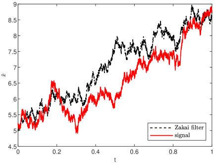
Figure 1: The Zakai filter and signal for $\lambda=3$.

In addition, we simulate a sample path for only continuous observation $Y_{t}$ with $\lambda=0$ and mixed observations of $Y_{t}$ and $Z_{t}$ with $\lambda=3$. We trace their corresponding conditional standard deviation versus time $t$, see Fig. 2. It shows that including information on point process observation reduces the conditional standard deviation.

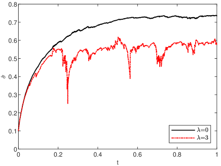
Figure 2: The conditional standard deviation

We fix $T=0.25$, $\lambda=2$ and a stepsize $\kappa=N^{-1}=2^{-20}$ and then compute $m=500$ reference ’exact’ sample paths. Simultaneously we compute $m$ Zakai filter approximate solutions for each stepsize $\kappa_{i}=N_{i}^{-1}=2^{-i}$ with $i=16,17,18,19$. Define an error function

$$d(\kappa_{i})=\{\frac{1}{N_{i}m}\sum_{r=1}^{N_{i}}\sum\limits_{j=1}^{m}|\hat{X}^{j}(t_{r})-\hat{X}_{r}^{j}|^{2}\}^{1/2}.$$

The dynamic behavior of the errors as varying stepsize $\kappa_{i}$ is exhibited in Fig. 3, demonstrating the half order convergence rate.

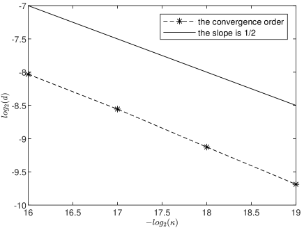
Figure 3: The convergence order of the splitting-up method.

Example 2. Consider a nonlinear filtering model

$$dX_{t}=\sin(X_{t})dt+2dw_{t},\quad X_{0}\sim\mathcal{N}(5,0.01),$$

$$dY_{t}=5.5X_{t}dt+0.5dw_{t}+dv_{t},\quad Y_{0}=0,$$

$$Z_{t}~{}\text{is a doubly stochastic Poisson process with the intensity of}~{}\lambda X_{t}^{2}.$$

The corresponding Zakai equation is

$$dp(t)= (2\frac{\partial^{2}p(t)}{\partial x^{2}}-\sin(x)\frac{\partial p(t)}{\partial x}-\cos(x)p(t)-(\lambda x^{2}-1)p(t))dt$$

$$+(-\frac{2}{5}\sqrt{5}\frac{\partial p(t)}{\partial x}+\frac{11}{5}\sqrt{5}xp(t))dY_{t}+(\lambda x^{2}-1)p(t-)dZ_{t}.$$

Set $\lambda=3$, $T=0.5$, $\kappa=0.5\times 10^{-5}$. We trace a sample signal trajectory using our Zakai filter and depict the approximations in Fig. 4.

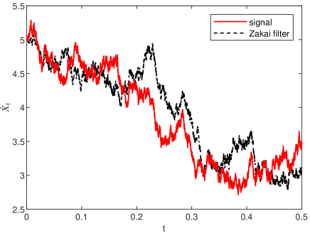
Figure 4: The Zakai filter and signal process.

Next, we verify the convergence order in a temporal variable. We compute $m=500$ reference “exact" Zakai filter solutions by fixing the stepsize $\kappa=2^{-20}$. Then we calculate $m$ numerical Zakai filter solutions for each stepsize $\kappa_{i}=2^{-i}$, $i=14,15,16,17$. We plot the errors in $\log$-$\log$ scale, cf. Fig. 5, which shows that the convergence order is of $\frac{1}{2}$.

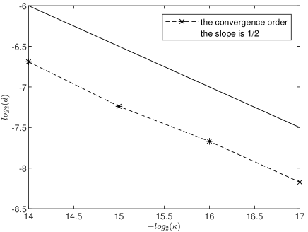
Figure 5: The convergence order of time discretized method.

6 Conclusion and discussion

In this paper, we considered a nonlinear filtering model with observations involving a mixture of a Wiener process and a point process. After deriving the corresponding Zakai equation, we constructed the splitting-up scheme where the Zakai equation is decomposed into three equations: A deterministic PDE, an SDE driven by a Wiener process, and an SDE driven by a point process. Then we discretized these equations in the temporal direction by finite difference methods. By estimating the errors of these splitting up equations and the errors of the temporal discretization, we derived the half-order convergence result for the proposed numerical scheme using Milstein’s fundamental theorem on numerical methods for SDEs. Our current work focuses on semi-discretizations in time. Future research on this topic includes the construction and error estimates for fully discretized numerical schemes.

Acknowledgments The research was partly supported by the National Key R&D Program (2020YFA0714101, 2020YFA0713601), NSFC (12171199, 11971198), Jilin Provincial Department of science and technology (20210201015GX).

References

- \bibcommenthead
- (1) Dawson, P., Gailis, R., Meehan, A.: Detecting disease outbreaks using a combined bayesian network and particle filter approach. Journal of theoretical biology 370, 171–183 (2015)
- (2) Mitter, S.K.: On the analogy between mathematical problems of nonlinear filtering and quantum physics. Ricerche Automat. 10(2), 163–216 (1979)
- (3) Yang, T., Huang, G., Mehta, P.G.: Joint probabilistic data association-feedback particle filter for multiple target tracking applications. In: 2012 American Control Conference (ACC), pp. 820–826 (2012). IEEE
- (4) Anadranistakis, M., Lagouvardos, K., Kotroni, V., Elefteriadis, H.: Correcting temperature and humidity forecasts using kalman filtering: Potential for agricultural protection in northern greece. Atmospheric research 71(3), 115–125 (2004)
- (5) Das, S.: Computational Business Analytics. CRC Press, Boca Raton (2013). https://doi.org/10.1201/b16358
- (6) Young, L., Young, J.: Statistical Ecology, (1998). https://doi.org/10.1007/978-1-4757-2829-3
- (7) Frey, Rüdiger and Schmidt, Thorsten: Pricing and hedging of credit derivatives via the innovations approach to nonlinear filtering. Finance Stoch. 16(1), 105–133 (2012). https://doi.org/10.1007/s00780-011-0153-0
- (8) Frey, R., Schmidt, T., Xu, L.: On Galerkin approximations for the Zakai equation with diffusive and point process observations. SIAM J. Numer. Anal. 51(4), 2036–2062 (2013). https://doi.org/10.1137/110837395
- (9) Brémaud, P.: A Martingale Approach to Point Processes vol. 345. University of California, Berkeley (1972)
- (10) Frey, R., Schmidt, T.: Pricing corporate securities under noisy asset information. Math. Finance 19(3), 403–421 (2009). https://doi.org/10.1111/j.1467-9965.2009.00374.x
- (11) Aggoun, L.: Robust filtering and detection of an insurance model. Stoch. Dyn. 7(1), 91–102 (2007). https://doi.org/10.1142/S0219493707001949
- (12) Ceci, C., Colaneri, K., Cretarola, A.: Local risk-minimization under restricted information on asset prices. Electron. J. Probab. 20, 96–30 (2015). https://doi.org/10.1214/EJP.v20-3204
- (13) Qiao, H., Duan, J.: Nonlinear filtering of stochastic dynamical systems with Lévy noises. Adv. in Appl. Probab. 47(3), 902–918 (2015). https://doi.org/10.1239/aap/1444308887
- (14) Fernando, B.P.W., Hausenblas, E.: Nonlinear filtering with correlated Lévy noise characterized by copulas. Braz. J. Probab. Stat. 32(2), 374–421 (2018). https://doi.org/10.1214/16-BJPS347
- (15) Zakai, M.: On the optimal filtering of diffusion processes. Zeitschrift für Wahrscheinlichkeitstheorie und verwandte Gebiete 11(3), 230–243 (1969)
- (16) Bensoussan, A., Glowinski, R., Răşcanu, A.: Approximation of the Zakai equation by the splitting up method. SIAM J. Control Optim. 28(6), 1420–1431 (1990). https://doi.org/10.1137/0328074
- (17) Florchinger, P., le Gland, F.: Time-discretization of the zakai equation for diffusion processes observed in correlated noise. Stochastics and Stochastic Reports 35(4), 233–256 (1991) https://doi.org/10.1080/17442509108833704. https://doi.org/10.1080/17442509108833704
- (18) Gyöngy, I., Krylov, N.: On the splitting-up method and stochastic partial differential equations. Ann. Probab. 31(2), 564–591 (2003). https://doi.org/10.1214/aop/1048516528
- (19) Ito, K.: Approximation of the Zakai equation for nonlinear filtering. SIAM J. Control Optim. 34(2), 620–634 (1996). https://doi.org/10.1137/S0363012993254783
- (20) Bao, F., Cao, Y., Webster, C., Zhang, G.: A hybrid sparse-grid approach for nonlinear filtering problems based on adaptive-domain of the Zakai equation approximations. SIAM/ASA J. Uncertain. Quantif. 2(1), 784–804 (2014). https://doi.org/10.1137/140952910
- (21) Florchinger, P., Le Gland, F.: Time-discretization of the Zakai equation for diffusion processes observed in correlated noise. Stochastics Stochastics Rep. 35(4), 233–256 (1991). https://doi.org/10.1080/17442509108833704
- (22) Le Gland, F.: Splitting-up approximation for SPDEs and SDEs with application to nonlinear filtering. In: Stochastic Partial Differential Equations and Their Applications (Charlotte, NC, 1991). Lect. Notes Control Inf. Sci., vol. 176, pp. 177–187. Springer, Berlin (1992). https://doi.org/10.1007/BFb0007332. https://doi.org/10.1007/BFb0007332
- (23) Protter, P.E.: Stochastic Integration and Differential Equations. Stochastic Modelling and Applied Probability, vol. 21, p. 419. Springer, Berlin (2005). https://doi.org/%****␣ACOM_Nov.bbl␣Line␣375␣****10.1007/978-3-662-10061-5. Second edition. Version 2.1, Corrected third printing. https://doi.org/10.1007/978-3-662-10061-5
- (24) Bain, A., Crisan, D.: Fundamentals of Stochastic Filtering. Stochastic Modelling and Applied Probability, vol. 60, p. 390. Springer, New York (2009). https://doi.org/10.1007/978-0-387-76896-0. https://doi.org/10.1007/978-0-387-76896-0
- (25) Pardoux, E.: Équations du filtrage non linéaire, de la prédiction et du lissage. Stochastics 6(3-4), 193–231 (1981/82). https://doi.org/10.1080/17442508208833204
- (26) Revuz, D., Yor, M.: Continuous Martingales and Brownian Motion, 3rd edn. Grundlehren der Mathematischen Wissenschaften [Fundamental Principles of Mathematical Sciences], vol. 293, p. 602. Springer, Berlin (1999). https://doi.org/10.1007/978-3-662-06400-9. https://doi.org/10.1007/978-3-662-06400-9
- (27) Shreve, S.E.: Stochastic Calculus for Finance. II. Springer Finance, p. 550. Springer, New York (2004). Continuous-time models
- (28) Liptser, R.S., Shiryaev, A.N.: Statistics of Random Processes. I, expanded edn. Applications of Mathematics (New York), vol. 5, p. 427. Springer, Berlin (2001). General theory, Translated from the 1974 Russian original by A. B. Aries, Stochastic Modelling and Applied Probability
- (29) Bensoussan, A.: On a general class of stochastic partial differential equations. Stochastic Hydrology & Hydraulics 1(4), 297–302 (1987)
- (30) Pardoux, E.: Stochastic partial differential equations and filtering of diffusion processes. Stochastics 3(2), 127–167 (1979). https://doi.org/10.1080/17442507908833142
- (31) Da Prato, G., Kunstmann, P.C., Lasiecka, I., Lunardi, A., Schnaubelt, R., Weis, L.: Functional Analytic Methods for Evolution Equations. Lecture Notes in Mathematics, vol. 1855, p. 472. Springer, Berlin (2004). https://doi.org/10.1007/b100449. Edited by M. Iannelli, R. Nagel and S. Piazzera. https://doi.org/10.1007/b100449
- (32) Gawarecki, L., Mandrekar, V.: Stochastic Differential Equations in Infinite Dimensions with Applications to Stochastic Partial Differential Equations. Probability and its Applications (New York), p. 291. Springer, Heidelberg (2011). https://doi.org/10.1007/978-3-642-16194-0. https://doi.org/10.1007/978-3-642-16194-0
- (33) Milstein, G.N.: Numerical Integration of Stochastic Differential Equations. Mathematics and its Applications, vol. 313, p. 169. Kluwer Academic Publishers Group, Dordrecht (1995). https://doi.org/10.1007/978-94-015-8455-5. Translated and revised from the 1988 Russian original. https://doi.org/10.1007/978-94-015-8455-5
- (34) Kanagawa, S.: Error estimations for the Euler-Maruyama approximate solutions of stochastic differential equations. Monte Carlo Methods Appl. 1(3), 165–171 (1995). https://doi.org/10.1515/mcma.1995.1.3.165
- (35) Kloeden, P.E., Platen, E.: Numerical Solution of Stochastic Differential Equations, pp. 8–12. Springer, New York (2005)
- (36) Shen, J., Tang, T., Wang, L.-L.: Spectral Methods: Algorithms, Analysis and Applications vol. 41. Springer, London (2011)