Dynamic Kernel Sparsifiers

A geometric graph associated with a set of points $P=\{x_{1},x_{2},\cdots,x_{n}\}\subset\mathbb{R}^{d}$ and a fixed kernel function $\mathsf{K}:\mathbb{R}^{d}\times\mathbb{R}^{d}\to\mathbb{R}_{\geq 0}$ is a complete graph on $P$ such that the weight of edge $(x_{i},x_{j})$ is $\mathsf{K}(x_{i},x_{j})$. We present a fully-dynamic data structure that maintains a spectral sparsifier of a geometric graph under updates that change the locations of points in $P$ one at a time. The update time of our data structure is $n^{o(1)}$ with high probability, and the initialization time is $n^{1+o(1)}$. Under certain assumption, we can provide a fully dynamic spectral sparsifier with the robostness to adaptive adversary.

We further show that, for the Laplacian matrices of these geometric graphs, it is possible to maintain random sketches for the results of matrix vector multiplication and inverse-matrix vector multiplication in $n^{o(1)}$ time, under updates that change the locations of points in $P$ or change the query vector by a sparse difference.

1 Introduction

Kernel methods are a fundamental tool in modern data analysis and machine learning, with extensive applications in computer science, from clustering, ranking and classification, to ridge regression , principal-component analysis and semi-supervised learning [vL07, NJW02, Zhu05a, Zhu05b, LSZ⁺19]. Given a set of $n$ points in $\mathbb{R}^{d}$ and a nonnegative function $\mathsf{K}:\mathbb{R}^{d}\times\mathbb{R}^{d}\rightarrow\mathbb{R}_{\geq 0}$, a kernel matrix has the form that the $i,j$-th entry in the matrix is $\mathsf{K}(x_{i},x_{j}).$

Kernel matrices and linear-systems naturally arise in modern machine learning and optimization tasks, from Kernel PCA and ridge regression [AM15, ACW17, AKM⁺17, LSS⁺20], to Gaussian-process regression (GPR) [RN10]), federated learning [KMY⁺16], and the ‘state-space model’ (SSM) for dynamic sequence modeling in deep learning [GJG⁺21, GGR21]. In most of these applications, the underlying data points $x_{i}$ are dynamically changing across iterations, either by nature or by design, and therefore computational efficiency of linear-algebraic operations in this setting requires dynamic algorithms to maintain the kernel matrix under insertions and deletions of data points.

• Dynamic spectral clustering. Take a kernel matrix as an adjacency matrix of a weighted graph. In the static setting, a common approach [NJW02] for spectral clustering is to run spectral clustering algorithm on the new and approximate sparse Laplacian matrix of the weighted graph instead of the original weighted graph. In the dynamic setting, the a small fraction of data points come and leave. To keep the spectral clustering, it is inefficient to rebuild the sparse spectral sparsifier every time when data gets changed, and thus dynamically maintaining the sparse spectral sparsifier is preferred.

• Dynamic $n$-body simulation. In physics and astronomy, an N-body simulation [TH08] is a simulation of a dynamical system of particles, usually under the influence of physical forces, such as gravity. Let $P\subset\mathbb{R}^{d}$ denote a set of points. Then for every $i\in[d]$, we let $G_{i}$ be a graph on the points in $P$. Let $C_{g}$ denote the gravitational constant and $m_{x}$ denote the mass of point $x\in P$, then for any two points $u,v\in P$, the non-negative weight/kernel function of the edge $(u,v)$ is defined as $\mathsf{K}_{i}(u,v):=(\frac{C_{g}\cdot m_{u}\cdot m_{v}}{\|u-v\|_{2}^{2}})\cdot(\frac{|v_{i}-u_{i}|}{\|u-v\|_{2}})$ . In order to find the force between the points, we write the weighted adjacency matrix of $G_{i}$ as $A_{i}$. Then in static setting, it is easy to get the force by computing $A_{i}{\bf 1}$. In the dynamic setting, since those $n$-bodies are slowly moving over the time, we prefer to dynamically maintaining it instead of re-computing it from scratch every time.

• Dynamic semi-supervised learning. In semi-supervised learning tasks, we have a prior knowledge of the value of a function on a subset. The task is to extend the function to the rest part of the set such that the weighted sum of difference. . Formally, we are given a function $f:P\rightarrow\mathbb{R}$ together with its value on some subset $X\subset P$. Then we aim to extend the function $f$ to the whole set $P$, which can minimize $\sum_{u,v\in P,u\neq v}\mathsf{K}(u,v)(f(u)-f(v))^{2}$ [Zhu05b]. In static setting, solving a Laplacian system on the geometric graph on $P$ leads to the solution of the function $f$. In the dynamic setting, the points are changing over the time, thus, we want to maintain the solution of Laplacian system solve.

Many major techniques for these problems use tools in spectral graph theory on a special class of dense graphs called geometric graphs. For a function $\mathsf{K}:\mathbb{R}^{d}\times\mathbb{R}^{d}\rightarrow\mathbb{R}$ and a set of points $P\subset\mathbb{R}^{d}$, the $\mathsf{K}$-graph on $P$ is a complete graph on vertex set $P$, where the weight of edge $(u,v)$ is $\mathsf{K}(u,v)$ for $u,v\in P$. For the aforementioned applications, it is natural to adopt tools from the dynamic geometric graph problems. Dynamic spectral sparsification, dynamic matrix-vector multiplication, and dynamic Laplacian system solving in geometric graphs are the tools we can utilize for the problems above.

We use $G$ to denote the geometric graph on $n$ points in Euclidean space. Let $L_{G}$ be the Laplacian matrix of $G$. [ACSS20] presented an algorithm to construct a $\epsilon$-spectral sparsifier of $G$, denoted by $H$ ($(1-\epsilon)L_{G}\preceq L_{H}\preceq(1+\epsilon)L_{G}$) in almost linear time (without explicitly writing down the $n^{2}$ dense graph/matrix).

In this work, we study the following questions

Given a set of $n$ points $P\subset\mathbb{R}^{d}$ and a function $\mathsf{K}$, is there a dynamic algorithm that can update the spectral sparsifier of the geometric graph $G$ on $P$ and $\mathsf{K}$ in sublinear time, where in each iteration the location of one existing point in $P$ gets changed? In addition, can we maintain an approximation to the matrix vector multiplication result of this Laplacian matrix, and an approximation to the inversion of this Laplacian matrix, both in sublinear time?

Prior to this work, no dynamic algorithm exists for geometric graphs (in terms of kernel function). Fully dynamic $(1\pm\epsilon)$-spectral edge sparsifiers algorithm exists for general graphs [ADK⁺16]. In [ADK⁺16], the sparisifer can be maintained in amortized $\mathrm{poly}(\log(n),1/\epsilon)$ time per update. However, in the setting of geometric graphs, each point update would result in the weight change of $O(n)$ edges. Therefore, the cost of directly applying the the edge sparsifier update algorithm can be high in this scenario.

We formally write down our problem as follows:

Definition 1.1 (Dynamic spectral sparsifier of geometric graph).

Given a set of points $P\subset\mathbb{R}^{d}$ and kernel function $\mathsf{K}:\mathbb{R}^{d}\times\mathbb{R}^{d}\rightarrow\mathbb{R}_{\geq 0}$. Let $G$ denote the geometric graph on to $P$ with edge weight $w(x_{i},x_{j}):=\mathsf{K}(x_{i},x_{j})$. Let $L_{G}$ be the Laplacian matrix of graph $G$. Let $\epsilon\in(0,0.1)$ denote an accuracy parameter. We want to design a data structure that dynamically maintains a $(1\pm\epsilon)$-spectral sparsifier for $G$ and supports the following operations:

• Initialize$(P\subset\mathbb{R}^{d},\epsilon\in(0,0.1))$, this operation takes point set $P$ and constructs a $(1\pm\epsilon)$-spectral sparsifier of $L_{G}$.

• Update$(i\in[n],z\in\mathbb{R}^{d})$, this operation takes a vector $z$ as input, and to replace $x_{i}$ (in point set $P$) by $z$, in the meanwhile, we want this update to be fast and the change in the spectral sparsifier to be small.

For the above problem, we focus our attention on kernel functions with a natural property called $(C,L)$-multiplicatively Lipschitz. For $C\geq 1$ and $L\geq 1$, we say a function is $(C,L)$-Lipschitz if that, for all $c\in[1/C,C]$, it holds that $\frac{1}{c^{L}}\leq\frac{f(cx)}{f(x)}\leq c^{L}$.

Definition 1.2 (Sketch of approximation to matrix multiplication).

Given a geometric graph $G$ with respect to point set $P$ and kernel function $\mathsf{K}$, and an $n$-dimensional vector $v$, we want to maintain a low dimensional sketch of an approximation to the multiplication result $L_{G}v$, where an $\varepsilon$-approximation to multiplication result $Mx$ is a vector $b$ such that $\|b-Mx\|_{M^{\dagger}}\leq\varepsilon\|Mx\|_{M^{\dagger}}$.

Definition 1.3 (Sketch of approximation to Laplacian solving).

Given a geometric graph $G$ with respect to point set $P$ and kernel function $\mathsf{K}$, and an $n$-dimensional vector $b$, we want to maintain a low dimensional sketch of an approximation to the multiplication result $L_{G}^{\dagger}b$.

We here explain the necessity of maintaining a sketch of an approximation instead of the directly maintaining the multiplication result in the dynamic regime. Let the underlying geometry graph on $n$ vertices be $G$ and the vector be $v\in\mathbb{R}^{n}$. When a $d$-dimensional point is moved in the geometric graph, a column and a row are changed $L_{G}$. We can assume the first row and first column are changed with no loss of generality. When this happens, if the first entry of $v$ is not 0, all entries will change in the multiplication result. Therefore, it takes at least $\Omega(n)$ time to update the multiplication result exactly. In order to spend subpolynomial time to maintain the multiplication result, we need to reduce the dimension of vectors. Therefore, we use a sketch matrix with $m=\mathrm{poly}\log(n)$ rows. In addition, dynamic algorithms has been widely used in many of the optimization tasks. Usually, most optimization analysis are robust against noises and errors, such as linear programming [CLS19, JSWZ21], semidefinite programming [HJS⁺21] and sum of squares method [JNW22]. Approximate solutions are sufficient to for these optimizations.

1.1 Our Results

For the dynamic sparsifier problem, we show that there is an algorithm to maintain the spectral sparsifier of a geometric graph in subpolynomial time.

Theorem 1.4 (Informal version of Theorem 4.3).

Let $\mathsf{K}$ denote a $(C,L)$-multiplicative Lipschitz kernel function. For any given data point set $P\subset\mathbb{R}^{d}$ with size $n$, there is a randomized dynamic algorithm that receives updates of locations of points in $P$ one at a time, and maintains a almost linear spectral sparsifier in $n^{o(1)}$ time with probability $1-1/\mathrm{poly}(n)$.

By making extra assumptions on dimensions, we can provide result for adversarial setting

Theorem 1.5 (Informal version of Theorem 8.5 ).

Let $\mathsf{K}$ denote a $(C,L)$-multiplicative Lipschitz kernel function. For any given data point set $P\subset\mathbb{R}^{d}$ with size $n$, if $\alpha^{d}=O(\mathrm{poly}(n))$, then there is a randomized dynamic algorithm that receives updates of locations of points in $P$ one at a time, and maintains a almost linear spectral sparsifier in $n^{o(1)}$ time with probability $1-1/\mathrm{poly}(n)$. It also supports adversarial updates.

For the dynamic matrix-vector multiplication problem, we give an algorithm to maintain a sketch of the multiplication between the Laplacian matrix of a geometric graph and a given vector in subpolynomial time.

Theorem 1.6 (Informal version of Theorem 5.1).

Let $G$ be a $(C,L)$-Lipschitz geometric graph on $n$ points. Let $v$ be a vector in $\mathbb{R}^{n}$. There exists an data structure Multiply that maintains a vector $\widetilde{z}$ that is a low dimensional sketch of an approximation to the multiplication result $L_{G}\cdot v$. Multiply supports the following operations:

• UpdateG$(x_{i},z)$: move a point from $x_{i}$ to $z$ and thus changing $\mathsf{K}_{G}$ and update the sketch. This takes $n^{o(1)}$ time.

• UpdateV$(\delta_{v})$: change $v$ to $v+\delta_{v}$ and update the sketch. This takes $n^{o(1)}$ time.

• Query: return the up-to-date sketch.

We also present a dynamic algorithm to maintain the sketch of the solution to a Laplacian system.

Theorem 1.7 (Informal version of Theorem  6.1).

Let $G$ be a $(C,L)$-Lipschitz geometric graph on $n$ points. Let $b$ be a vector in $\mathbb{R}^{n}$. There exists an data structure Solve that maintains a vector $\widetilde{z}$ that is a low dimensional sketch of an $\varepsilon$-approximation to the multiplication result $L_{G}^{\dagger}\cdot b$. It supports the following operations:

• UpdateG$(x_{i},z)$: move a point from $x_{i}$ to $z$ and thus changing $\mathsf{K}_{G}$ and update the sketch. This takes $n^{o(1)}$ time

• UpdateB$(\delta_{b})$: change $b$ to $b+\delta_{b}$ and update the sketch. This takes $n^{o(1)}$ time.

• Query: return the up-to-date sketch

2 Technical Overview

2.1 Fully Dynamic Kernel Sparsification Data Structure

A geometric graph w.r.t. kernel function $\mathsf{K}:\mathbb{R}^{d}\times\mathbb{R}^{d}\to\mathbb{R}$ and points $x_{1},\ldots,x_{n}\in\mathbb{R}^{d}$ is a graph on $x_{1},\ldots,x_{n}$ where the weight of the edge between $x_{i}$ and $x_{j}$ is $\mathsf{K}(x_{i},x_{j})$. An update to a geometric graph occurs when the location of one of these points changes.

In a geometric graph, when an update occurs, the weights of $O(n)$ edges change. Therefore, directly applying the existing algorithms for dynamic spectral sparsifiers ([ADK⁺16]) to update the geometric graph spectral sparsifier will take $\Omega(n)$ time per update. However by using the fact that the points are located in $\mathbb{R}^{d}$ and exploiting the properties of the kernel function, we can achieve faster update.

Before presenting our dynamic data structure, we first have a high level idea of the static construction of the geometric spectral sparsifier, which is presented in [ACSS20].

2.1.1 Building Blocks of the Sparsifier

In order to construct a spectral sparsifier more efficiently, one can partition the graph into several subgraphs such that the edge weights on each subgraph are close. On each of these subgraphs, leverage score sampling, which is introduced in [SS11] and used for constructing sparsifiers, can be approximated by uniform sampling.

For a geometric graph built from a $d$-dimensional point set $P$, under the assumption that each edge weight is obtained from a $(C,L)$-Lipschitz kernel function (Definition 3.1), each edge weight in the geometric graph is not distorted by a lot from the euclidean distance between the two points (Lemma 3.20). Therefore, we can compute this partition efficiently with by finding a well separated pair decomposition (WSPD, Definition 3.13) of the given point set.

A $s$-WSPD of $P$ is a collection of well separated (WS) pairs $(A_{i},B_{i})$ such that for all $a\neq b\in P$, there is a pair $(A,B)$ satisfying $a\in A,b\in B$, and the distance between $A$ and $B$ is at least $s$ times the diameters of $A$ and $B$ ($A$ and $B$ are $s$-well separated, see Figure 1). Therefore, the distance between $A$ and $B$ is a $(1+1/s)$-multiplicative approximation of the distance between any point in $A$ and any point in $B$ and each WS pair in the WSPD can be viewed as a unweighted biclique (complete bipartite graph). On an unweighted biclique, uniform random sampling and leverage score sampling are equivalent. Therefore, a uniformly random sample of the biclique forms a spectral sparsifier of the biclique, and union of the sampled edges from all bicliques form a spectral sparsifier of the geometric graph (See Figure 2 and Figure 3).

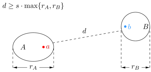
Figure 1: An $s$-well separated (WS) pair. In this figure, for two points $a,b\in P$, there exists a pair $A,B\subseteq P$ such that $a\in A,b\in B$, and the distance between $A$ and $B$ is at least $s$ times the diameter of $A$ and $B$, i.e., $d\geq s\cdot\max\{r_{A},r_{B}\}$.

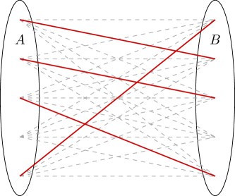
Figure 2: $\{A,B\}$ is a WS pair, which can be viewed as an unweighted biclique. The red edges is uniformly sampled from the biclique, which forms a spectral sparsifier of the biclique.

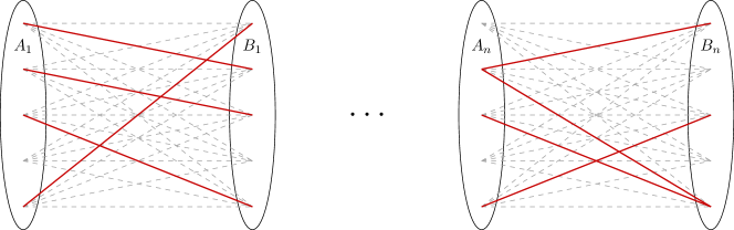
Figure 3: $\{A_{i},B_{i}\}$ is the WS pairs in the WSPD of the data set $P$. Hence, by uniformly sampling from each of the WS pairs, the union of the sampled edges forms a spectral sparsifire of the whole geometric graph.

However, the time needed for constructing a WSPD is exponentially dependent on the ambient dimension of the point set and thus WSPD cannot be computed efficiently when the dimension is high. To solve this problem, one can use the ultra low dimensional Johnson Lindenstrauss (JL) projection to project the point set down to $k=o(\log n)$ dimension such that with high probability the distance distortion (multiplicative difference between the distance between two points and the distance between their low dimensional images) between any pair of points is at most $n^{C_{\mathrm{jl}}\cdot(1/k)}$, where $C_{\mathrm{jl}}$ is a constant. This distortion becomes an overestimation of the leverage score in the resulting biclique, and can be compensated by sampling $n^{C_{\mathrm{jl}}\cdot(1/k)}$ edges. Then one can perform a $2$-WSPD on the $k$-dimensional points. Since JL projection gives a bijection between the $d$-dimensional points and their $k$-dimensional images, a $2$-WSPD of the $k$-dimensional point set gives us a canonical $(2\cdot n^{C_{\mathrm{jl}}(1/k)})$-WSPD of the $d$-dimensional point set $P$. This $(2\cdot n^{C_{\mathrm{jl}}(1/k)})$-WSPD of $P$ is what we use to construct the sparsifier.

In summary, when received a set of points $P$, we first use the ultra-low dimensional JL projection to project these points to an $k=o(\log n)$ dimensional space, run a 2-WSPD on the $k$-dimensional points, and then map the WSPD result back to obtain a $(2\cdot n^{C_{\mathrm{jl}}(1/k)})$-WSPD of $P$. For each pair $(A,B)$ in this $d$-dimensional WSPD, we randomly sample edges from the Biclique$(A,B)$, which denotes the complete bipartite graph with $A$ and $B$ being two sides. The union of all sampled edges is a spectral sparsifier of the geometric graph on $P$.

2.1.2 Dynamic update of the Geometric Spectral Sparsifier.

For a geometric graph build on point set $P$, we want the above spectral sparsifier to be able to handle the following update :

Point location change $(x_{i}\in P,z\in\mathbb{R}^{d})$: move the point from location $x_{i}$ to location $z$. This is equivalent to removing point $x\in P$ and then adding $z$ to $P$.

However, in order to update the geometric spectral sparsifier efficiently, there are a few barriers that we need to overcome.

Updating WSPD

When point set $P$ changes, we want to update the WSPD such that the number of WS pairs that are changed in the WSPD is small. [FHP05] presented an algorithm to update the list of WS pairs, but it cannot be used directly in this situation. To see why, we need to summarize how a WSPD is computed from a hierarchical point partition called the compressed quad tree.

Given a $d$-dimensional point set $P$, we can assume it’s a subset of $[0,1)^{d}$ with no loss of generality. We can build a tree structure $Q$ called the quad tree on $P$ in the following way

• The root of $Q$ is the region $[0,1)^{d}$.

• For each node $n$ in $Q$, if $n$ contains at least 2 points in $P$, we equally divide $n$ along $d$ axes and obtain $2^{d}$ subregions, for each subregion that contains points in $P$ we create a child of $n$ with this region.

• For each node $n$ in $Q$ that contains only 1 point in $P$, $n$ is a leaf node with no children. Note that all regions containing only 1 point are leaves, and all leaves contain only 1 point.

Note that in a quad tree, there can be a long chain of tree nodes that contains the same set of points. We replace this chain by the first and last nodes on the chain with an edge between them and obtain a compressed quad tree, denoted by $T$.

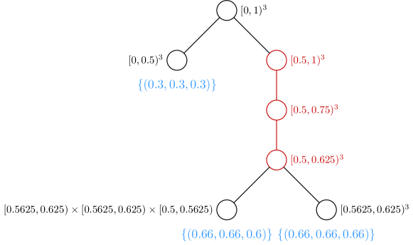
(a) An example of quad tree

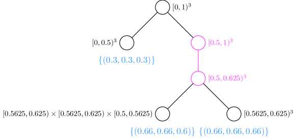
(b) An example of compressed quad tree

Figure 4: An example of quad tree and compressed quad tree: Consider a set of points $P=\{(0.3,0.3,0.3),(0.66,0,66,0,6),(0.66,0.66,0.66)\}\subseteq\mathbb{R}^{3}$. Figure (a) shows the (full) quad tree built on $P$ and figure (b) shows the compressed quad tree built on $P$. The difference is that, the red chain of nodes in (a) is replaced by the two cyan nodes in (b).

Recall that a pair of point sets are $s$-well separated if and only if the distance between the two point sets are at least $s$ times the diameters of them. Since each quad tree node corresponds to a non-empty subset of $P$, with a compressed quad tree $T$ of $P$, a WSPD of $P$ can be constructed as a list of pairs of tree nodes in $T$. We build this WSPD in a greedy way, that is, we try to find well separated pairs of tree nodes of $T$ that are as close to the root (denoted by $r$) as possible. Specifically, we start from examining tree node pair $(r,r)$. When examining pair $(u,v)$, if they are well separated, we add this pair to the WSPD. Otherwise, we assume the diameter of $v$ is smaller than the diameter of $u$ and examine the pairs formed between $v$ and each child of $u$. Since singletons are always well separated, this process terminates. The WSPD obtained this way has the property that $(u,v)$ is in the WSPD only if the pair formed by their parents are not well separated.

Now we discuss how the WSPD can be maintained dynamically in [FHP05]. Here we only consider the case when a new point $x$ is added to $P$, because point deletion works in the same way. When a new point $x$ is added to $P$, the compressed quad tree changes in one of the following two ways (Figure 5):

• $x$ becomes a child of an existing quad tree node $u$

• $x$ is inserted between $u$ and its existing child $v$. In this case, we create a new quad tree node $w$ and let $x$ and $v$ be the children of $w$.

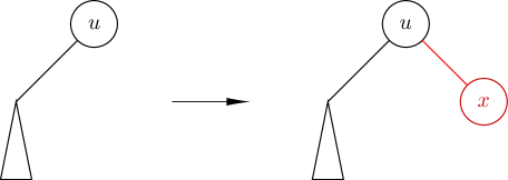
(a) Case 1 of insertion

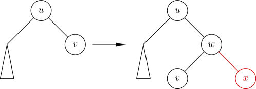
(b) Case 2 of insertion

Figure 5: Two cases after insertion. Figure (a) shows the condition when $x$ becomes a child of an existing tree node $u$. It is inserted directly. Figure (b) shows that $x$ lands in the same set of node $v$. The node $v$ is divided into three and let $w$ denote the generated root of $v$ and $x$. Here tree node $x$ corresponds to point set $\left\{x\right\}$. When there is no ambiguity, we use the name of a tree node to denote the point set it contains.

The dynamic algorithm in [FHP05] can only obtain a list of WS pairs such that $x$ or $w$ is one of the tree nodes in the pair. However, the new point $x$ is also added to all ancestors of $x$ in the compressed quad tree. In order to update the all bicliques containing point $x$, we need to also find all pairs such that the ancestors of $x$ or $w$ is one of the tree nodes in the pair.

Fortunately, the WSPD construction above has the property that each point $x$ appears only in $2^{O(k)}O(\log\alpha)$ WS pairs and we can find all these pairs in $2^{O(k)}O(\log\alpha)$ time (Section 4.4), where $\alpha=\max_{x,y\in P}\|x-y\|_{2}/\min_{x,y\in P}\|x-y\|_{2}$. This can be achieved by utilizing the compressed quad tree data structure. [HP11] proved the existence of a quad tree data structure that can (1) find the leaf node that contains a given point $x$, or the parent node under which the leaf node containing $x$ should be inserted if $x\not\in P$, (2) insert a leaf node containing a given point $x$, and (3) remove a leaf node containing a given point $x$, in $O(\log n)$ time. The WSPD can be stored in a list data structure that can find all WS pairs containing tree node $n$ for a given $n$ in time linear in the size of output.

With these tools, when a point location change occurs, and point $x_{i}$ is moved to $z$, we can do the following to find all WS pairs that need to be updated.

• Use the compressed quad tree data structure to locate leaf nodes that contains $x_{i}$ and $z$ (since $z$ is not in the point set before the update, we locate the parent node under which $z$ should be inserted)

• Go from each of these leaf nodes to the root of the compressed quad tree, for each tree node $n$ on this path, use the WSPD data structure to find all WS pairs containing $n$ and update this WS pair.

• Update these pairs and the compressed quad tree.

Algorithm 5 in Section 4.4 is a detailed version of this WSPD update scheme.

Resampling from bicliques.

When a point location change happens and point $x_{i}$ is moved to $z$, each pair $(A,B)$ in the WSPD list will undergo one and only one of the following changes,

• Remaining $(A,B)$

• Becoming $(A\backslash\left\{x_{i}\right\},B)$ or $(A,B\backslash\left\{x_{i}\right\})$

• Becoming $(A\cup\left\{z\right\},B)$ or $(A,B\cup\left\{z\right\})$

• Becoming $(A\backslash\left\{x_{i}\right\}\cup\left\{z\right\},B)$, $(A,B\backslash\left\{x_{i}\right\}\cup\left\{z\right\})$, $(A\backslash\left\{x_{i}\right\},B\cup\left\{z\right\})$ or $(A\cup\left\{z\right\},B\backslash\left\{x_{i}\right\})$

For each WS pair $(A,B)$ that remains $(A,B)$, we do not need to do anything about it. For each WS pair $(A,B)$ that is changed $(A^{\prime},B^{\prime})$, in order to maintain a spectral sparsifier of Biclique$(A^{\prime},B^{\prime})$, we need to find a new uniform sample from Biclique$(A^{\prime},B^{\prime})$. Simply drawing another uniform sample from $A^{\prime}\times B^{\prime}$ cannot be done fast enough when $|A^{\prime}\times B^{\prime}|$ is large and this resampling will cause a lot of edge weight changes in the final sparsifier, which is not optimal.

To overcome this barrier, suppose after an update, a WS pair $(A,B)$ is changed to $(A^{\prime},B^{\prime})$. Since the size difference between $A$ and $A^{\prime}$ and the size difference between $B$ and $B^{\prime}$ are at most constant, the size of $(A^{\prime}\times B^{\prime})\cap(A\times B)$ is much larger than the size of $(A^{\prime}\times B^{\prime})\backslash(A\times B)$. Therefore, when we draw a uniform sample from $A^{\prime}\times B^{\prime}$, most of the edges in the sample should be drawn from $(A^{\prime}\times B^{\prime})\cap(A\times B)$. Since we already have a uniform sample $E$ from $A\times B$, which contains a uniform sample from $(A^{\prime}\times B^{\prime})\cap(A\times B)$, we can reuse $E$ in the following way:

Let $H=E\cap(A^{\prime}\times B^{\prime})$. For each edge that needs to be samples, we flip an unfair coin for which the probability of landing on head is $\frac{|(A^{\prime}\times B^{\prime})\cap(A\times B)|}{|A^{\prime}\times B^{\prime}|}$, and we do the following (See Figure 7 for a visual example):

• If the coin lands on head, we sample an edge from $H$ without repetition;

• Otherwise we sample an edge from $(A^{\prime}\times B^{\prime})\backslash(A\times B)$ without repetition.

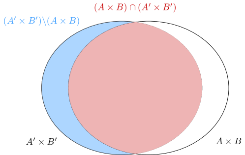
Figure 6: Division of the new biclique ($A^{\prime}\times B^{\prime}$): divided it into two parts (Blue part: $(A^{\prime}\times B^{\prime})\backslash(A\times B)$ and red part $(A\times B)\cap(A^{\prime}\times B^{\prime})$). And we sample from them respectively.

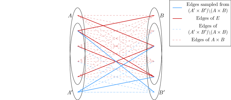
Figure 7: Resampling the biclique: $E$ (The red edges) is uniformly sampled from $\mathrm{Biclique}(A,B)$. After $A\times B$ becomes $A^{\prime}\times B^{\prime}$, we resample from $E\cap(A^{\prime}\times B^{\prime})$ with specific probabilities.

Algorithm 6 in Section 4.5 is a detailed version of this resampling scheme. With properly set probability for the coin flip, doing the sampling this way generates a uniform sample of $A^{\prime}\times B^{\prime}$, and with high probability, the difference between the new sample and $E$ is small.

However, in this process, although the difference between the new sample and $E$ is small, we still need to flip a coin for each new sample point. When the sample size is big, this can be slow.

The running time of resampling can be improved by removing a small number of edges from $E$. Indeed, suppose we want to resample $s$ edges from $A^{\prime}\times B^{\prime}$, the number of edges that need to be drawn from $(A^{\prime}\times B^{\prime})\backslash(A\times B)$ follows a Binomial distribution with parameters $s$ and $\frac{|(A^{\prime}\times B^{\prime})\backslash(A\times B)|}{|A^{\prime}\times B^{\prime}|}$. We have the following improved resampling algorithm:

Let $H=E\cap(A^{\prime}\times B^{\prime})$.

• Generate a random number $x$ under Binomial$(s,\frac{|(A^{\prime}\times B^{\prime})\backslash(A\times B)|}{|A^{\prime}\times B^{\prime}|})$;

• Remove $x+|H|-s$ pairs from $H$;

• Sample $x$ new edges uniformly from $(A^{\prime}\times B^{\prime})\backslash(A\times B)$ and add them to $H$.

Since $x$ has $n^{o(1)}$ expected value, with high probability (Markov inequality), $x$ is $n^{o(1)}$, the difference between $E$ and the new sample is $n^{o(1)}$, and the resampling process can be done in $n^{o(1)}$ time.

We omitted the edge case where the size of $H$ is less than $s-x$. Algorithm 7 in Section 4.6 is a detailed version of this sublinear resampling scheme.

Dynamic update.

Combining the above, we can update the spectral sparsifier (see Section 4.7 for details).

When a point location update occurs, suppose point $x_{i}$ is moved to $z$. We use the ultra low dimensional JL projection matrix to find the $O(k)$-dimensional images of $x_{i}$ and $z$. Then we update the $O(k)$-dimensional WSPD. For each $O(k)$-dimensional modified pair in the WSPD, we find the corresponding $d$-dimensional modified pairs, and resample edges from these $d$-dimensional modified pairs to update the spectral sparsifier. Since there are $2^{O(k)}\log\alpha$ modified pairs in each update and for each modified pair, with probability $1-\delta$, the uniform sample can be update in $O(\delta^{-1}\varepsilon^{-2}n^{o(1)})$ time, the dynamic update can be completed in $O(\delta^{-1}\varepsilon^{-2}n^{o(1)}\log\alpha)$ time per update.

2.2 Maintaining a sketch of an approximation to Laplacian matrix multiplication

Let $M$ be an $n\times n$ matrix and $x$ be a vector in $\mathbb{R}^{n}$. We say a vector $b$ is an $\epsilon$-approximation to $Mx$ if $\|x-Mx\|_{M^{\dagger}}\leq\epsilon\|Mx\|_{M^{\dagger}}$. Note that $\|x\|_{A}:=\sqrt{x^{\top}Ax}$.

Let $G$ be a graph and $H$ be a $\epsilon$-spectral sparsifier of $G$. By definition, this means $(1-\epsilon)L_{G}\preceq L_{H}\preceq(1+\epsilon)L_{G}$. Note that, if $A$ is a symmetric PSD matrix and symmetric $B$ is a matrix such that $(1-\epsilon)A\preceq B\preceq(1+\epsilon)A$, then we have $\|Bv-Av\|_{A^{\dagger}}\leq\epsilon\|Av\|_{A^{\dagger}}$ holds for all $v$.

Then, we have: Let $G$ be a graph on $n$ vertices and $H$ be a $\epsilon$-spectral sparsifier of $G$. For any $v\in\mathbb{R}^{n}$, $L_{H}v$ is an $\epsilon$-approximation of $L_{G}v$. Thus, to maintain a sketch of an $\epsilon$-approximation of $L_{G}x$, it suffices to maintain a sketch of $L_{H}x$.

The high level idea is to combine the spectral sparsifier defined in Section 4 and a sketch matrix to compute a sketch of the multiplication result $L_{H}v$ and try to maintain this sketch when the graph and the vector change.

We here justify the decision of maintaining a sketch instead of the directly maintaining the multiplication result. Let the underlying geometry graph on $n$ vertices be $G$ and the vector be $v\in\mathbb{R}^{n}$. When a point is moved in the geometric graph, a column and a row are changed in $L_{G}$. We can assume the first row and first column are changed with no loss of generality. When this happens, if the first entry of $v$ is not 0, all entries will change in the multiplication result. Therefore, it takes at least $\Omega(n)$ time to update the multiplication result. In order to spend subpolynomial time to maintain the multiplication result, we need to reduce the dimension of vectors. Therefore, we use a sketch matrix (with $m=\epsilon^{-2}\log(n/\delta)$ rows, see Definition 5.3 for details) to project vectors down to lower dimensions.

Maintaining the multiplication result efficiently.

In order to speed up the update, we generate two independent sketches $\Phi$ and $\Psi$, and maintain a sketch of $L_{H}$, denoted by $\widetilde{L}_{H}=\Phi L_{H}\Psi^{\top}$ and a sketch of $v$ denoted by $\widetilde{v}=\Psi v$. Since $\Phi$ and $\Psi$ are generated independently, in expectation $\Phi L_{H}\Psi^{\top}\Psi v=\Phi L_{H}v$. We store this result as the sketch (See Figure 8).

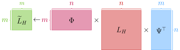
(a) The sketch of the Laplacian matrix

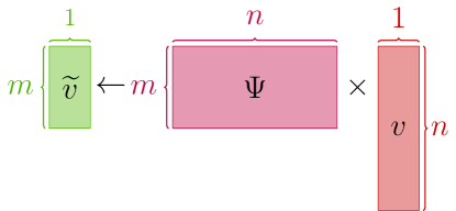
(b) The sketch of $v$

Figure 8: The sketch of the Laplacian matrix and the vector multiplied

Our spectral sparsifier has the property that with high probability, each update to the geometric graph $G$ incurs only a sparse changes in the sparsifier $H$, and this update can be computed efficiently. Therefore, when an update occurs to $G$, $\Delta L_{H}$ is sparse, so $\Phi\Delta L_{H}\Psi^{\top}$ can be computed efficiently. We use $\Phi\Delta L_{H}\Psi^{\top}$ to update the sketch (See Figure 9).

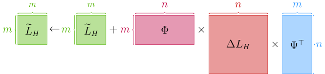
Figure 9: Updating the sketch

When a sparse update occurs to $v$, $\Psi\Delta v$ can be computed efficiently. Since $\widetilde{L}_{H}$ and $\Psi\Delta v$ are $m$-dimensional operator and vector, $\widetilde{L}_{H}\Psi\Delta v$ can be computed efficiently. We use $\widetilde{L}_{H}\Psi\Delta v$ to update the sketch.

2.3 Maintaining a sketch of an approximation to the solution of a Laplacian system

We start with another folklore fact If $(1-\epsilon)L_{G}\preceq L_{H}\preceq(1+\epsilon)L_{G}$, then $(1-2\epsilon)L_{G}^{\dagger}\preceq L_{H}^{\dagger}\preceq(1+2\epsilon)L_{G}^{\dagger}$.

Therefore, by using that fact, we have: Let $G$ be a graph on $n$ vertices and $H$ be a $\epsilon$-spectral sparsifier of $G$. For any vector $b$, $L_{H}^{\dagger}b$ is an $\epsilon$-approximation of $L_{G}^{\dagger}b$.

Thus, to maintain a sketch of an $\epsilon$-approximation of $L_{G}^{\dagger}x$, it suffices to maintain a sketch of $L_{H}^{\dagger}x$.

The high level idea is again to combine the spectral sparsifier defined in Section 4 and a sketch matrix to compute a sketch of the multiplication result $L_{H}^{\dagger}v$ and try to maintain this sketch when the graph and the vector change.

Caveat: using a different sketch.

When trying to maintain a sketch of a solution to $L_{H}x=b$, the canonical way of doing this is to maintain $\overline{x}$ such that $\Phi L_{H}\overline{x}=\Phi b$. However, here $\overline{x}$ is still an $n$-dimensional vector and we want to maintain a sketch with lower dimension. Therefore, we apply another sketch $\Psi$ to $\overline{x}$ and maintain $\widetilde{x}$ such that $\Phi L_{H}\Psi^{\top}\widetilde{x}=\Phi b$.

Maintaining the inversion result efficiently.

We maintain a sketch of $L_{H}$, denoted by $\widetilde{L}_{H}=\Phi L_{H}\Psi^{\top}$ and a sketch of $b$ denoted by $\widetilde{b}=\Phi b$. Since $\widetilde{L}_{H}$ is a $m$-dimensional operator, its pseudoinverse can be computed efficiently in $m^{\omega}$ time, where $\omega$ is the matrix multiplication constant. We use $\widetilde{L}_{H}^{\dagger}$ to denote the pseudoinverse of $\widetilde{L}_{H}$, and compute $\widetilde{L}_{H}\cdot\widetilde{b}$. We store this multiplication result as the sketch.

Our spectral sparsifier has the property that with high probability, each update to the geometric graph $G$ incurs only a sparse changes in the sparsifier $H$, and this update can be computed efficiently. Therefore, when an update occurs to $G$, $\Delta L_{H}$ is sparse, so $\Phi\Delta L_{H}\Psi^{\top}$ can be computed efficiently. We use $\Phi\Delta L_{H}\Psi$ to update the $\widetilde{L}_{H}$ and recompute $\widetilde{L}_{H}^{\dagger}$. We then update the sketch to $L_{H}^{\dagger}\cdot\widetilde{b}$ with the updated $L_{H}^{\dagger}$.

When a sparse update occurs to $b$, $\Phi\Delta b$ can be computed efficiently. Since $\widetilde{L}_{H}^{\dagger}$ and $\Phi\Delta b$ are $m$-dimensional operator and vector, $\widetilde{L}_{H}^{\dagger}\Phi\Delta b$ can be computed efficiently. We use $\widetilde{L}_{H}^{\dagger}\Psi\Delta b$ to update the sketch.

2.4 Adversary

In this section, we provide an overview of techniques we use for adversarial analysis.

2.4.1 Adversarial Distance Estimation

Let a random vector $V=(V_{1},V_{2},\cdots,V_{d})\in\mathbb{R}^{d}$ be sampled from Gaussian distribution and $U=\frac{1}{\|V\|}V$ be the normalized vector. Let vector $Z=(U_{1},U_{2},\cdots,U_{k})\in\mathbb{R}^{k}$ be the projection of $U$ onto the first $k$ components. From the properties of random variables sampled from Gaussian distribution, we can compute $\Pr[d(V_{1}^{2}+\cdots+V_{k}^{2})\leq k\beta(V_{1}^{2}+\cdots+V_{d}^{2})]$ via algebraic manipulations. Let $L=\|Z\|^{2}$. We show that when $\beta<1$, we have $\Pr[L\leq\frac{\beta k}{d}]\leq\exp(\frac{k}{2}(1-\beta+\ln\beta))$ and when $\beta\geq 1$, we have $\Pr[L\geq\frac{\beta k}{d}]\leq\exp(\frac{k}{2}(1-\beta+\ln\beta))$. By carefully choosing $\beta=n^{-2c/k}<1$, we can prove $\Pr[L\leq\frac{\beta k}{d}]\leq n^{-c}$. And when $\beta=n^{1/k}$, we can prove $\Pr[L\geq\frac{\beta k}{d}]\leq\exp(-\log^{1.9}n)$.

With the above analysis in hand, we can prove that there exists a map $f:\mathbb{R}^{d}\to\mathbb{R}^{k}$ such that for each fixed points $u,v\in\mathbb{R}^{d}$, we have

$$\|u-v\|_{2}^{2}\leq\|f(u)-f(v)\|_{2}^{2}\leq\exp(c_{0}\cdot\sqrt{\log n})\|u-v\|_{2}^{2}$$

with high success probability. We design a $\epsilon_{0}$-net of $\{x\in\mathbb{R}^{d}~{}|~{}\|x\|_{2}\leq 1\}$ denoted as $N$ which contains $|N|\leq(10/\epsilon_{0})^{O(\log n)}$ points (Here we assume $d=O(\log n)$). Then we prove that for all net points, the approximation guarantee still holds with high success probability via union bound. Finally, we want to generalize the distance estimation approximation guarantee to all points on the unit ball by quantizing the off-net point to its nearest on-net point. After rescaling the constant, we can obtain the same approximation guarantee with high probability.

Given a set of data points $\{x_{i}\}_{i=1}^{n}$, and a sketching matrix $\Pi\in\mathbb{R}^{k\times d}$ defined in Definition 7.1, we initialize a set of precomputed projected data points $\widetilde{x}_{i}=\Pi\cdot x_{i}$. To answer the approximate distance between a query point and all points in the data structure, we compute the distance as $u_{i}=n^{1/k}\cdot\sqrt{d/k}\cdot\|\widetilde{x}_{i}-\Pi q\|_{2}$ and prove it provides $\exp(\Theta(\sqrt{\log n}))$-approximation guarantee against adversarially chosen queries. When we need to update the $i$-th data point with a new vector $z\in\mathbb{R}^{d}$, we update $\widetilde{x}_{i}$ with $\Pi\cdot x_{i}$.

2.4.2 Sparsifier with robustness to adversarial updates

With the estimation robust for adversarial query, we are able to get a spectral sparsifier which supports adversarial updates of points, by applying the data structure in the construction of sparsifier (Setting the sketching dimension to be $O(\sqrt{\log n})$). Here we provide overview of our design to make it possible.

Net argument.

In order to make the distance estimation robust, one needs to argue that, for arbitrary point, it has high probability to have high precision. The data structure we use for distance estimation has a failure probability of $n^{-c}$, where $c$ is a constant we can set to be small. We can build an $\epsilon$-net $N$ with size of $|N|=\mathrm{poly}(n)$. Then by union bound over the net, the failure probability of distance estimation on the net is bounded by $n^{O(1)-c}$. Then by triangle inequality, we directly get the succeed probability guarantee for arbitrary point queries.

$\alpha$ and $d$ induce the size of the net.

From the discussion above, we note that, in order to make the $\epsilon$-net sufficient for union bound, it must have the size of $\mathrm{poly}(n)$. From another direction, we need to make that, all the points in the set are distinguishable in the nets, i.e., for two different points $A,B\in\mathbb{R}^{d}$, the closest points of the net to $A$ and $B$ are different. To make sure this, we must set the gap $\epsilon_{1}$ of the net to be less than the minimum distance of the points in the set. Without loss of generality, we first make the assumption that, all the points are in the $\ell_{2}$ unit ball of $\mathbb{R}^{d}$, i.e., the set $\{x\in\mathbb{R}^{d}~{}|~{}\|x\|_{2}\leq 1\}$. Then by the definition of aspect ratio $\alpha:=\frac{\max_{x,y\in P}d(x,y)}{\min_{x^{\prime},y^{\prime}\in P}d(x^{\prime},y^{\prime})}$, the minimum distance of the points in $P$ is $1/\alpha$. Thus, when we set the gap $\epsilon_{1}\leq C\cdot\alpha^{-1}$ for some constant $C$ small enough, every pair of points $x,y\in P$ is distinguishable in the net. Then there are $O(\alpha^{d})$ points in the net of the $\ell_{2}$ unit ball in $\mathbb{R}^{d}$ (See Figure 10).

Figure 10: The net argument in our problem. Let $d=2$. Here we restrict all the points to be in the $\ell_{2}$ unit ball. By the definition of aspect ratio $\alpha$, we know the minimum distance between two points is $1/\alpha$ ($A$ and $B$ in the figure). Thus, by setting $\epsilon=C\cdot\alpha^{-1}$ for some constant $C$ small enough, every pair of points is distinguishable.

Balancing the aspect ratio and dimension.

By the above paragraph, we know the set size is $O(\alpha^{d})$ to make the points distinguishable. Recall that, our distance estimation data structure has failure probability of $n^{-c}$. And in order to make the union bound sufficient for our net, we need to apply it over the $|N|^{2}$ pairs from $N$. That is, to make the total failure probability sufficient, we need to restrict $|N|=\mathrm{poly}(n)$. And in the former paragraphs, we already know that $|N|=O(\alpha^{d})$, thus we have the balancing constraint of the aspect ratio and dimension $\alpha^{d}=O(\mathrm{poly}(n))$.

Roadmap.

We divide the paper as follows. Section 3 gives the preliminary for our paper. Section 4 gives the fully dynamic spectral sparsifier for geometric graphs. Section 5 gives our sketch data structure for matrix multiplication. Section 6 introduces the algorithm for solving Laplacian system. Section 7 introduces the distance estimation data structure supporting adversarial queries. Based on that, Section 8 gives our spectral sparsifier that is robust to adaptive adversary.

3 Preliminary

3.1 Notations

For any two sets $A,B$, we use $A\triangle B$ to denote $(A\backslash B)\cup(B\backslash A)$. Given two symmetric matrices $A,B$, we say $A\preceq B$ if $\forall x$, $x^{\top}Ax\leq x^{\top}Bx$. For a vector $x$, we use $\|x\|_{2}$ to denote its entry-wise $\ell_{2}$ norm. For psd matrix $A$, we use $A^{\dagger}$ to denote the pseduo inverse of $A$. For two point sets $A,B$, we denote the complete bipartite graph on $A$ and $B$ by $\mathrm{Biclique}(A,B)$. We use $\mu_{n,i}$ to denote a elementary unit vector in $\mathbb{R}^{n}$ with $i$-th entry $1$ and others $0$.

3.2 Definitions

We define the $(C,L)$-Lipschitz function as follows:

Definition 3.1.

For $C\geq 1$ and $L\geq 1$, a function is $(C,L)$-Lipschitz if for all $c\in[1/C,C]$,

$$\frac{1}{c^{L}}\leq\frac{f(cx)}{f(x)}\leq c^{L}.$$

We define the Laplacian of a graph:

Definition 3.2 (Laplacian of graph).

Let $G=(V,E,w)$ be a connected weighted undirected graph with $n$ vertices and $m$ edges, together with a positive weight function $w:E\rightarrow\mathbb{R}_{+}$. If we orient the edges of $G$ arbitrarily, we can write its Laplacian as

$$L_{G}=A^{\top}WA,$$

where $A\in\mathbb{R}^{m\times n}$ is the signed edge-vertex incidence matrix, given by

$$A(e,v)=\begin{cases}1,~{}~{}~{}&\text{if }v\text{ is the head of }e\\ -1&\text{if }v\text{ is the tail of }e\\ 0&\text{otherwise}\end{cases}$$

and $W\in\mathbb{R}_{+}^{m\times m}$ is the diagonal matrix such that $W(e,e)=w(e)$, for all $e\in E$. We use $\{a_{e}\}_{e\in E}$ to denote the row vectors of $A$.

It follows obviously that $L_{G}$ is positive semidefinite since for any $x\in\mathbb{R}^{n}$,

$$x^{\top}L_{G}x=x^{\top}A^{\top}WAx=\|W^{1/2}Ax\|_{2}^{2}\geq 0.$$

Since $L_{G}$ is symmetric, we can diagnolize it and write

$$L_{G}=\sum_{i=1}^{n-1}\lambda_{i}u_{i}u_{i}^{\top},$$

where $\lambda_{1},\dots,\lambda_{n-1}$ are the nonzero eigenvalues of $L_{G}$ and $u_{1},\dots,u_{n-1}$ are the corresponding orthonormal eigenvectors. The Moore-Penrose Pseudoinverse of $L_{G}$ is

$$L_{G}^{\dagger}:=\sum_{i=1}^{n-1}\frac{1}{\lambda_{i}}u_{i}u_{i}^{\top}.$$

3.3 Basic Algebra

Fact 3.3 (Folklore).

Let $\epsilon\in(0,1/2)$. Given two PSD matrix $A$ and $B$ such that

$$(1-\epsilon)A\preceq B\preceq(1+\epsilon)A$$

then we have:

• $(1+\epsilon)^{-1}A^{\dagger}\preceq B^{\dagger}\preceq(1-\epsilon)^{-1}A^{\dagger}$

• $\|Bx-Ax\|_{A^{\dagger}}\leq\epsilon\|Ax\|_{A^{\dagger}},\forall x.$

3.4 Johnson-Linderstrauss Transform

3.4.1 Untral-low Dimension JL

Lemma 3.4 (Ultralow Dimensional Projection [JL84, DG03]).

For $k=o(\log n)$, with high probability at least $1-1/\mathrm{poly}(n)$ the maximum distortion in pairwise distance obtained from projecting $n$ points into $k$ dimensions (with appropriate scaling) is at most $n^{O(1/k)}$, e.g.,

$$\|x-y\|_{2}\leq\|f(x)-f(y)\|_{2}\leq n^{O(1/k)}\cdot\|x-y\|_{2}$$

where $f$ is the projection from $\mathbb{R}^{d}$ to $\mathbb{R}^{k}$.

Throughout this paper, we use $C_{\mathrm{jl}}$ to denote the constant on the exponent, i.e. the distortion is bounded above by $n^{C_{\mathrm{jl}}\cdot(1/k)}$.

Lemma 3.5 ([JL84, DG03]).

Let $k<d$. Let $V_{1},V_{2},\cdots,V_{d}$ be $d$ independent Gaussian $N(0,1)$ random variables, $V=(V_{1},V_{2},\cdots,V_{d})$, and let $U=\frac{1}{\|V\|}V$. Let the vector $Z=(U_{1},U_{2},\cdots,U_{k})\in\mathbb{R}^{k}$ be the projection of $U$ onto the first $k$ components and let $L=\|Z\|^{2}$ be the square of the norm of $Z$. Then

• Part 1. If $\beta<1$, then

  $$\Pr[L\leq\frac{\beta k}{d}]\leq\beta^{k/2}\cdot(1+\frac{(1-\beta)k}{(d-k)})^{(d-k)/2}\leq\exp(\frac{k}{2}(1-\beta+\ln\beta))$$

• Part 2. If $\beta>1$, then

  $$\Pr[L\geq\frac{\beta k}{d}]\leq\beta^{k/2}\cdot(1+\frac{(1-\beta)k}{(d-k)})^{(d-k)/2}\leq\exp(\frac{k}{2}(1-\beta+\ln\beta))$$

3.4.2 Useful lemmas on JL

Using Lemma 3.5, we can show that

Lemma 3.6.

Let $\beta=n^{1/k}$, then we have $\Pr[L\geq\frac{\beta k}{d}]\leq\exp(-\frac{1}{4}kn^{1/k})\leq\exp(-\log^{1.9}n)$.

Proof.

We show that

$$\Pr[L\geq\frac{\beta k}{d}]\leq ~{}\exp(\frac{k}{2}(1-\beta+\ln\beta))$$

$$\leq ~{}\exp(-\frac{k}{2}\frac{\beta}{2})$$

$$= ~{}\exp(-\frac{k}{2}\frac{n^{1/k}}{2})$$

$$\leq ~{}\exp(-\log^{1.9}n)$$

where the first step follows from Lemma 3.5, the second step follows from $\beta/2\geq 1+\ln\beta$, the third step follows from $\beta=n^{1/k}$, and the last step follows from $n^{1/k}\geq\log^{1.9}n$. ∎

Using Lemma 3.5 and choosing parameter $\beta$ carefully, we can show that:

Lemma 3.7.

Let $\beta=n^{-2c/k}/e=2^{-2c(\log n)/k}/e<1$, then we have $\Pr[L\leq\frac{\beta k}{d}]\leq n^{-c}$.

Proof.

We show that

$$\Pr[L\leq\frac{\beta k}{d}]\leq ~{}\beta^{k/2}\cdot(1+\frac{(1-\beta)k}{(d-k)})^{(d-k)/2}$$

$$= ~{}\beta^{k/2}\cdot(1+\frac{(1-\beta)k}{(d-k)})^{\frac{(d-k)}{k(1-\beta)}\cdot\frac{k(1-\beta)}{2}}$$

$$\leq ~{}\beta^{k/2}\cdot e^{k/2}$$

$$\leq ~{}(\beta/e)^{k/2}$$

$$\leq ~{}n^{-c}$$

where the first step comes from Lemma 3.5, the second step follows that $(d-k)/2=\frac{(d-k)}{k(1-\beta)}\cdot\frac{k(1-\beta)}{2}$, the third step follows $(1+\frac{1}{a})^{a}=e$ and $\frac{k(1-\beta)}{2}\leq\frac{k}{2}$, the fourth step simplifies the term, and the last step follows from $\beta=n^{-2c/k}/e$.

∎

3.5 Well Separated Pair Decomposition (WSPD)

We assume that throughout the process, all points land in $[0,1]^{d}$ and the aspect ratio of the point set is at most $\alpha$.

Definition 3.8.

The aspect ratio ($\alpha$) of a point set $P$ is

$$\alpha:=\frac{\max_{x,y\in P}d(x,y)}{\min_{x^{\prime},y^{\prime}\in P}d(x^{\prime},y^{\prime})}.$$

We state several standard definitions from literature [CK95].

Definition 3.9 (Bounding rectangle).

Let $P\subset\mathbb{R}^{d}$ be a set of points, we define the bounding rectangle of $P$, denoted as $R(P)$, to be the smallest rectangle in $\mathbb{R}^{d}$ such that encloses all points in $P$, where “rectangle” means some cartesian product $[x_{1},x_{1}^{\prime}]\times[x_{2},x_{2}^{\prime}]\times\dots\times[x_{d},x_{d}^{\prime}]\in\mathbb{R}^{n}$. For all $i\in[d]$, We define the length of $R$ in $i$-th dimension by $l_{i}(R):=x_{i}^{\prime}-x_{i}$. We denote $l_{\max}(R):=\max_{i\in[d]}l_{i}(R)$ and $l_{\min}(R):=\min_{i\in[d]}l_{i}(R)$. When $l_{i}(R)$ are all equal for $i\in[d]$, we say $R$ is a $d$-cube, and denote its length by $l(R)$. For any set of points $P\subseteq\mathbb{R}^{d}$, we denote $l_{i}(P)=l_{i}(R(P))$.

Definition 3.10 (Well separated point sets).

Point sets $P,Q$ are well separated with separation $s$ if $R(P)$ and $R(Q)$ can be contained in two balls of radius $r$, and the distance between these two balls is at least $s\cdot r$, where we say $s$ is the separation.

Definition 3.11 (Interaction product).

The interaction product of point sets $P,Q$, denoted by $P\otimes Q$ is defined as

$$P\otimes Q:=\left\{\left\{p,q\right\}\mid p\in P,q\in Q,p\neq q\right\}$$

Definition 3.12 (Well separated realization).

Let $P,Q\subseteq\mathbb{R}^{d}$ be two sets of points. A well separated realization of $P\otimes Q$ is a set $\left\{(P_{1},Q_{1}),\ldots,(P_{k},Q_{k})\right\}$ such that

1. $P_{i}\subset P$, $Q_{i}\subset Q$ for all $i\in[k]$.

2. $P_{i}\cap Q_{i}=\emptyset$ for all $i\in[k]$.

3. $P\otimes Q=\bigcup_{i=1}^{k}P_{i}\otimes Q_{i}$.

4. $P_{i}$ and $Q_{i}$ are well-separated.

5. $\left(P_{i}\otimes Q_{i}\right)\cap\left(P_{j}\otimes Q_{j}\right)=\emptyset$ for $i\neq j$.

Throughout the paper, we will mention that a set $P$ is associated with a binary tree $T$. Here we mean the tree $T$ has leaves labeled by a set containing only one point which is in $P$. All the non-leaf nodes are labeled by the union of the sets labeled with its subtree.

Given set $P\subseteq\mathbb{R}^{d}$, let $T$ be a binary tree associated with $P$. For $A,B\subseteq P$, we say that a realization of $A\otimes B$ uses $T$ if all the $A_{i}$ and $B_{i}$ in the realization are nodes in $T$.

Definition 3.13 (Well separated pair decomposition).

A well separated pair decomposition (WSPD) of a point set $P$ is a structure consisting of a binary tree $T$ associated with $P$ and a well separated realization of $P\otimes P$ uses $T$.

The result of [CK95, HP11] states that for a point set $P$ of $n$ points, a well separated pair decomposition of $P$ of $O(n)$ pairs can be computed in $O(n\log n)$ time. There are two steps of computing a well separated decomposition: (1) build compressed quad tree (defined below in Definition 3.15) for the given point set; (2) find well separated pairs from the tree (Algorithm 1).

Definition 3.14 (Quad tree).

Given a point set $P\subset[0,1)^{d}$, a tree structure $\mathcal{T}$ can be constructed in the following way:

• The root of $\mathcal{T}$ is the region $[0,1)^{d}$

• For each tree node $n\in\mathcal{T}$, we can obtain $2^{d}$ subregions by equally dividing $n$ into two halves along each of the $d$ axes. The children of $n$ in $\mathcal{T}$ are the subregions that contain points in $P$. $n$ has at most $2^{d}$ children.

• The dividing stops when there is only one point in the cell.

In a quad tree, we define the degree of a tree node to be the number of children it has. There can be a lot of nodes in $T$ that has degree 1. Particularly, there can be a path of degree one nodes. Every node on this path contain the same point set. To reduce the size of the quad tree, we compress these degree one paths.

Definition 3.15 (Compressed quad tree).

Given a quad tree $T$, for each a path of degree one nodes, we replace it with the first and last nodes on the path, with one edge between them. We call this resulting tree a compressed quad tree.

Lemma 3.16 (Chapter 2 in [HP11]).

The compressed quad tree data structure $T$ has the following properties:

• Given a point $p$, $p$ exists in at most $O(\log\alpha)$ quad tree nodes.

• The height of the tree is $O(\min(n,\log\alpha))$.

$T$ supports the following operations:

• QTFastPL$(T,p)$ returns the leaf node containing $p$, or the parent node under which $\left\{p\right\}$ should be inserted if $p$ does not exist in $T$, in $O(\log n)$ time.

• QTInsertP$(T,p)$ adds $p$ to the $T$ in $O(\log n)$ time.

• QTDeleteP$(T,p)$ removes $p$ from $T$ in $O(\log n)$ time.

Lemma 3.17 (Theorem 2.2.3 in [HP11]).

Given a $d$-dimensional point set $P$ of size $n$, a compressed quad tree of $P$ can be constructed in $O(dn\log n)$ time.

Algorithm 1 Finding well separated pairs

1:procedure WSPD($Q,u,v$) $\triangleright$ $Q$ is a compressed quad tree, $u,v$ are tree nodes on $Q$, Lemma 3.19

2:     if $u$ and $v$ are well separated then

3:         return $(u,v)$

4:     else

5:         if $l_{\max}(u)>l_{\max}(v)$ then

6:              Let $u_{1},\ldots,u_{m}$ denote the children of $u$

7:              return $\bigcup_{i}\text{WSPD}(Q,u_{i},v)$

8:         else

9:              Let $v_{1},\ldots,v_{m}$ denote the children of $v$

10:              return $\bigcup_{i}\text{WSPD}(Q,u,v_{i})$

11:         end if

12:     end if

13:end procedure

14:

15:procedure ComputeWSPD($Q$)$\triangleright$ $Q$ is a compressed quad tree

16:     $r\leftarrow$ root of $Q$

17:     return WSPD$(Q,r,r)$

18:end procedure

Theorem 3.18 ([CK95]).

For point set $P\subseteq\mathbb{R}^{d}$ of size $n$ and $s>1$, a $s$-WSPD of size $O(s^{d}n)$ can be found in $O(s^{d}n+n\log n)$ time and each point is in at most $2^{O(d)}\log\alpha$ pairs.

Lemma 3.19 ([CK95, HP11]).

Given a compressed quad tree $Q$ of $n$ points in $\mathbb{R}^{d}$, two nodes $u,v$ in the tree $Q$. The procedure ComputeWSPD (Algortihm 1) generates the WSPD from the tree $Q$, and runs in time

$$O(n\times 2^{d}\log n).$$

3.6 Properties of $(C,L)$-Lipschitz Functions

Lemma 3.20 (Lemma 6.8 in [ACSS20]).

Let $G$ be a graph and $G^{\prime}$ be another graph on the same set of vertices with different edge weights satisfying

$$\frac{1}{K}w_{G^{\prime}}(e)\leq w_{G}(e)\leq Kw_{G^{\prime}}(e)$$

Let $f:\mathbb{R}\rightarrow\mathbb{R}$ be a $(C,L)$-lipschitz kernel function (Definition 3.1), for some $C<K$. Let $f(G)$ be the graph obtained by switching each edge weight from $w(e)$ to $f(w(e))$. Then,

$$\frac{1}{K}w_{G^{\prime}}(e)\leq w_{G}(e)\leq Kw_{G^{\prime}}(e).$$

3.7 Leverage Score and Effective Resistance

Definition 3.21.

Given a matrix $A\in\mathbb{R}^{m\times n}$, we define $\sigma\in\mathbb{R}^{m}$ to denote the leverage score of $A$, i.e.,

$$\sigma_{i}=a_{i}^{\top}(A^{\top}A)a_{i},\forall i\in[m].$$

Let $(G,V,E)$ be an graph obtained by arbitrarily orienting the edges of an undirected graph, with $n$ points and $m$ edges, together with a weight function $w:E\rightarrow\mathbb{R}_{+}$. We now describe the electrical flows on the graph. We let vector $I_{\mathrm{ext}}\in\mathbb{R}^{n}$ denote the currents injected at the vertices. Let $I_{\mathrm{edge}}\in\mathbb{R}^{m}$ denote currents induced in the edges (in the direction of orientation) and $V\in\mathbb{R}^{n}$ denotes the potentials induced at the vertices. Let $A,W$ be defined as Definition 3.2. By Kirchoff’s current law, the sum of the currents entering a vertex is equal to the amount injected at the vertex, i.e.,

$$A^{\top}I_{\mathrm{edge}}=I_{\mathrm{ext}}.$$

By Ohm’s law, the current flow in an edge is equal to the potential difference across its ends times its conductance, i.e.,

$$I_{\mathrm{edge}}=WAV.$$

Combining the above, we have that

$$I_{\mathrm{ext}}=A^{\top}(WAV)=L_{G}V.$$

If $I_{\mathrm{ext}}\bot\mathrm{Span}(1_{n})=\mathrm{ker}(K)$, that is, the total amount of current injected is equal to the total amount extracted, then we have that

$$V=L_{G}^{\dagger}I_{\mathrm{ext}}.$$

Definition 3.22 (Leverage score of a edge in a graph).

We define the effective resistance or leverage score between two vertices $u$ and $v$ to be the potential difference between them when a unit current is injected at one that extracted at the other.

Lemma 3.23 (Algebraic form of leverage score, [SS11]).

Let $(G,E,V)$ be a graph described as above, for any edge $e\in E$, the leverage score (effective resistance) of $e$ has the following form

$$R(e)=AL_{G}^{\dagger}A^{\top}(e,e),$$

where the matrix $A,L_{G}$ is defined as Definition 3.2.

Proof.

We now derive an algebraic expression for the effective resistance in terms of $L_{G}^{\dagger}$. For a edge $e\in E$, we use $R(e)$ to denote its effective resistance. To inject and extract a unit current across the endpoints of an edge $(u,v)$, we set $I_{\mathrm{ext}}=a_{e}^{\top}$, which is clearly orthogonal to $1_{n}$. The potentials induced by $I_{\mathrm{ext}}$ at the vertices are given by $V=L_{G}^{\dagger}a_{e}^{\top}$. To measure the potential difference across $e=(u,v)$, we simply multiply by $a_{e}$ on the left:

$$V_{v}-V_{u}=(\mu_{n,v}-\mu_{n,u})^{\top}V=a_{e}L_{G}^{\dagger}a_{e}^{\top}.$$

It follows that, the effective resistance across $e$ is given by $a_{e}L_{G}^{\dagger}a_{e}^{\top}$ and that the matrix $AL_{G}^{\dagger}A^{\top}$ has its diagonal entries $AL_{G}^{\dagger}A^{\top}(e,e)=R(e)$. ∎

3.8 Spectral sparsifier

Here we give the formal definition of spectral sparsifier of a graph:

Definition 3.24 (Spectral sparsifier).

Given an arbitrary undirected graph $G$, let $L_{G}$ denote the Laplacian (Definition 3.2) of $G$. We say $H$ is a $\epsilon$-spectral sparsifier of $G$ if

$$(1-\epsilon)L_{G}\preceq L_{H}\preceq(1+\epsilon)L_{G}.$$

4 Fully Dynamic Spectral Sparsifier for Geometric Graphs in Sublinear Time

A geometric graph w.r.t. kernel function $\mathsf{K}:\mathbb{R}^{d}\times\mathbb{R}^{d}\to\mathbb{R}$ and points $x_{1},\ldots,x_{n}\in\mathbb{R}^{d}$ is a graph on $x_{1},\ldots,x_{n}$ where the weight of the edge between $x_{i}$ and $x_{j}$ is $\mathsf{K}(x_{i},x_{j})$. An update to a geometric graph occurs when the location of one of these points changes.

In a geometric graph, when an update occurs, the weights of $O(n)$ edges change. Therefore, directly applying the existing algorithms for dynamic spectral sparsifiers ([ADK⁺16]) to update the geometric graph spectral sparsifier will take $\Omega(n)$ time per update. However by using the fact that the points are located in $\mathbb{R}^{d}$ and exploiting the properties of the kernel function, we can achieve faster update.

Before presenting our dynamic data structure, we first have a high level idea of the static construction of the geometric spectral sparsifier, which is presented in [ACSS20].

Building Blocks of the Sparsifier.

In order to construct a spectral sparsifier more efficiently, one can partition the graph into several subgraphs such that the edge weights on each subgraph are close. On each of these subgraphs, leverage score sampling, which is introduced in [SS11] and used for constructing sparsifiers, can be approximated by uniform sampling.

For a geometric graph built from a $d$-dimensional point set $P$, under the assumption that each edge weight is obtained from a $(C,L)$-Lipschitz kernel function (Definition 3.1), each edge weight in the geometric graph is not distorted by a lot from the euclidean distance between the two points (Lemma 3.20). Therefore, we can compute this partition efficiently by finding a well separated pair decomposition (WSPD, Definition 3.13) of the given point set.

A $s$-WSPD of $P$ is a collection of well separated (WS) pairs $(A_{i},B_{i})$ such that for all $a\neq b\in P$, there is a pair $(A,B)$ satisfying $a\in A,b\in B$, and the distance between $A$ and $B$ is at least $s$ times the diameters of $A$ and $B$ ($A$ and $B$ are $s$-well separated). Therefore, the distance between $A$ and $B$ is a $(1+1/s)$-multiplicative approximation of the distance between any point in $A$ and any point in $B$ and each WS pair in the WSPD can be viewed as a unweighted biclique (complete bipartite graph). On an unweighted biclique, uniform random sampling and leverage score sampling are equivalent. Therefore, a uniformly random sample of the biclique forms a spectral sparsifier of the biclique, and union of the sampled edges from all bicliques form a spectral sparsifier of the geometric graph.

However, the time needed for constructing a WSPD is exponentially dependent on the ambient dimension of the point set and thus WSPD cannot be computed efficiently when the dimension is high. To solve this problem, one can use the ultra low dimensional Johnson Lindenstrauss (JL) projection to project the point set down to $k=o(\log n)$ dimension such that with high probability the distance distortion (multiplicative difference between the distance between two points and the distance between their low dimensional images) between any pair of points is at most $n^{C_{\mathrm{jl}}\cdot(1/k)}$, where $C_{\mathrm{jl}}$ is a constant. This distortion becomes an overestimation of the leverage score in the resulting biclique, and can be compensated by sampling $n^{C_{\mathrm{jl}}\cdot(1/k)}$ edges. Then one can perform a $2$-WSPD on the $k$-dimensional points. Since JL projection gives a bijection between the $d$-dimensional points and their $k$-dimensional images, a $2$-WSPD of the $k$-dimensional point set gives us a canonical $(2\cdot n^{C_{\mathrm{jl}}(1/k)})$-WSPD of the $d$-dimensional point set $P$. This $(2\cdot n^{C_{\mathrm{jl}}(1/k)})$-WSPD of $P$ is what we use to construct the sparsifier.

Dynamic Update of the Geometric Spectral Sparsifier.

We present the following way to update the above sparsifier. In order to do this, we need to update the ultra low dimensional JL projection, the WSPD and the sampled edges from each biclique. In order to update JL projection for $O(n)$ updates, we initialize the JL projection matrix with $O(n)$ points so that with high probability, the distortion is small for $O(n)$ updates.

To update the WSPD, we note that each point appears only in $O(\log\alpha)$ WS pairs and we can find all these pairs in $2^{O(k)}\log\alpha$ time (Section 4.4).

To update the sampled edges, Algorithm 7 updates the old sample to a new one such that with high probability, the number of edges changed in the sample is at most $n^{o(1)}$ and this can be done in $n^{o(1)}$ time (Section 4.6).

Combining the above, we can update the spectral sparsifier (Section 4.7).

Making the Data Structure Fully Dynamic.

Below is the layout of this section.

• In Section 4.1, we provide some definitions.

• In Section 4.2, we define the members of our data structure.

• In Section 4.3, we present the algorithm for initialization.

• In Section 4.4 we state an algorithm to find modified pairs in WSPD when a point’s location is changed.

• In Section 4.5, we first propose a (slow) resampling algorithm takes $O(n)$ time to resample $n^{o(1)}$ edges.

• In Section 4.6, we then explain how to improve the running time of (slow) resampling algorithm

• In Section 4.7, we prove the correctness of our update procedure.

• In Section 4.8, we apply a black box reduction to our update algorithm to obtain a fully dynamic update algorithm.

4.1 Definitions

We define our problem as follows:

Definition 4.1 (Restatement of Definition 1.1).

Given a set of points $P\subset\mathbb{R}^{d}$ and kernel function $\mathsf{K}:\mathbb{R}^{d}\times\mathbb{R}^{d}\rightarrow\mathbb{R}_{\geq 0}$. Let $G$ denote the geometric graph that is corresponding to $P$ with the $(i,j)$ edge weight is $w_{i,j}:=\mathsf{K}(x_{i},x_{j})$. Let $L_{G,P}$ denote the Laplacian matrix of graph $G$. Let $\epsilon\in(0,0.1)$ denote an accuracy parameter. The goal is to design a data structure that dynamically maintain a $(1\pm\epsilon)$-spectral sparsifier for $G$ and supports the following operations:

• Initialize$(P\subset\mathbb{R}^{d},\epsilon\in(0,0.1))$, this operation takes point set $P$ and constructs a $(1\pm\epsilon)$-spectral sparsifier of $L_{G}$.

• Update$(i\in[n],z\in\mathbb{R}^{d})$, this operation takes a vector $z$ as input, and to replace $x_{i}$ (in point set $P$) by $z$, in the meanwhile, we want to spend a small amount of time and a small number of changes to spectral sparisifer so that

Definition 4.2 (Restatement of Definition 3.8).

Given a set of points $P=\{x_{1},\cdots,x_{n}\}\subset\mathbb{R}^{d}$. We define the aspect ratio $\alpha$ of $P$ to be

$$\alpha:=\frac{\max_{i,j}\|x_{i}-x_{j}\|_{2}}{\min_{i,j}\|x_{i}-x_{j}\|_{2}}.$$

The main result we want to prove in this section is

Theorem 4.3 (Formal version of Theorem 1.4).

Let $\alpha$ be the aspect ratio of a $d$-dimensional point set $P$ defined above. Let $k=o(\log n)$. There exists a data structure DynamicGeoSpar that maintains a $\epsilon$-spectral sparsifier of size $O(n^{1+o(1)})$ for a $(C,L)$-Lipschitz geometric graph such that

• DynamicGeoSpar can be initialized in

  $$O(ndk+\epsilon^{-2}n^{1+o(L/k)}\log n\log\alpha)$$

  time.

• DynamicGeoSpar can handle point location changes. For each change in point location, the spectral sparsifier can be updated in

  $$O(dk+2^{O(k)}\epsilon^{-2}n^{o(1)}\log\alpha)$$

  time. With high probability, the number of edges changed in the sparsifier is at most

  $$\epsilon^{-2}2^{O(k)}n^{o(1)}\log\alpha.$$

4.2 The Geometric Graph Spectral Sparsification Data Structure

Definition 4.4.

In DynamicGeoSpar, we maintain the following objects:

• $P$: a set of points in $\mathbb{R}^{d}$

• $\mathcal{H}$: an $n^{1+o(1)}$ size $\epsilon$-spectral sparsifier of the geometric graph generated by kernel $\mathsf{K}$ and points $P$

• $\Pi$: a JL projection matrix

• $Q$: the image of $P$ after applying projection $\Pi$

• $T$: a quad tree of point set $Q$

• $\mathcal{P}$: a WSPD for point set $Q$ obtained from $P$

• Edges: a set of tuples $(A_{i},B_{i},E_{i})$. $E_{i}$ is a set of edges uniformly sampled from Biclique$(X_{i},Y_{i})$, where $X_{i}$ and $Y_{i}$ are the $d$-dimensional point sets corresponding to $A_{i}$ and $B_{i}$ respectively

Algorithm 2 Data Structure

1:data structure DynamicGeoSpar $\triangleright$ Theorem 4.3

2:members $\triangleright$ Definition 4.4

3:     ${\cal H}$ $\triangleright$ An $n^{1+o(1)}$ size sparsifier

4:     $P\subset\mathbb{R}^{d}$$\triangleright$ A point set for the geometric graph

5:     $\Pi\in\mathbb{R}^{k\times d}$ $\triangleright$ Projection matrix

6:     $Q\subset\mathbb{R}^{k}$ $\triangleright$ A set of $k=o(\log n)$ dimensional points obtained by applying $\Pi$ to all points in $P$

7:     $T$$\triangleright$ A quad tree generated from $P^{\prime}$

8:     $\mathcal{P}=\left\{(A_{i},B_{i})\right\}_{i=1}^{m}$ $\triangleright$ A WSPD of $P$ based on $T$

9:     $\textsc{Edges}=\left\{(A_{i},B_{i},E_{i})\right\}_{i=1}^{m}$$\triangleright$ $E_{i}$ is a set of edges sampled from biclique $(X_{i},Y_{i})$, where $X_{i}$ and $Y_{i}$ are the $d$-dimensional point sets

10:end members

11:end data structure

4.3 Initialization

Here in this section, we assume that kernel function $\mathsf{K}(x,y)=f(\|x-y\|_{2}^{2})$ is $(C,L)$-Lipschitz (Definition 3.1).

Algorithm 3 DynamicGeoSpar

1:data structure DynamicGeoSpar $\triangleright$ Theorem 4.3

2:procedure Initialize($P,\epsilon,\delta,\mathsf{K}$) $\triangleright$ Lemma 4.5

3:     $P\leftarrow P$

4:     $\Pi\leftarrow$ a random $(k\times d)$ JL-matrix $\triangleright$ Lemma 3.4

5:     $Q\leftarrow\left\{\Pi\cdot p\mid p\in P\right\}$

6:     $T\leftarrow$ build a compressed quad tree for $Q$ $\triangleright$ Lemma 3.17

7:     $\mathcal{P}\leftarrow$ WSPD$(T,\text{root}(T),\text{root}(T))$$\triangleright$ Algorithm 1

8:     $\textsc{Edges},\mathcal{H}\leftarrow\textsc{InitSparsifier}(\mathcal{P},\mathsf{K},\epsilon,k)$ $\triangleright$ Algorithm 4

9:end procedure

10:end data structure

Lemma 4.5.

Let $\alpha\geq 0$ be defined as Definition 3.8. Initialize$(P\subset\mathbb{R}^{d},\epsilon\in(0,0.1),\delta\in(0,0.1),\mathsf{K})$ (Algorithm 3) takes a $d$-dimensional point set $P$ as inputs and runs in

$$O(ndk+\epsilon^{-2}n^{1+O(L/k)}2^{O(k)}\log n\log\alpha)$$

time, where $k$ is the JL dimension, $k=o(\log n)$.

Proof.

The running time consists of the following parts:

• Line 4 and Line 5 takes time $O(ndk)$ to Generate the projection matrix and compute the projected sketch;

• By Lemma 3.17, Line 6 takes time

  $$O(nk\log n);$$

  to build the quad tree.

• By Lemma 3.19, Line 7 takes time

  $$O(n\times 2^{k}\log n)$$

  to generate the WSPD.

• By Lemma 4.7, Line 8 takes time

  $$O(\epsilon^{-2}n^{1+O(L/k)}2^{o(k)}\log n\log\alpha)$$

  to generate the sparsifier.

Adding them together we have the total running time is

$$O(ndk+\epsilon^{-2}n^{1+O(L/k)}2^{o(k)}\log n\log\alpha).$$

Thus we complete the proof.

∎

We here state a trivial fact of sampling edges from a graph.

Fact 4.6 (Random sample from a graph).

For any graph $G$ and a positive integer $s\in\mathbb{Z}_{+}$, there exists a random algorithm RandSample$(G,s)$ such that, it takes $G$ and $s$ as inputs, and outputs a set containing $s$ edges which are uniformly sampled from $G$ without replacement. This algorithm runs in time $O(s)$.

Now we are able to introduce the initialization algorithm for the sparsifier.

Algorithm 4 DynamicGeoSpar: init sparsifier.

1:data structure$\triangleright$ Theorem 4.3 DynamicGeoSpar

2:procedure InitSparsifer($\mathcal{P},\mathsf{K},\epsilon,k$) $\triangleright$ Lemma 4.7

3:     $\mathcal{H}\leftarrow$ empty graph with $n$ vertices

4:     $\textsc{Edges}\leftarrow\emptyset$

5:     for $(A,B)\in\mathcal{P}$ do

6:         Find $(X\subseteq P,Y\subseteq P)$ such that $X,Y$ are the $d$-dimensional point sets corresponding to $A,B$ respectively.

7:         $G\leftarrow$ Biclique$(\mathsf{K},X,Y)$

8:         $s\leftarrow\epsilon^{-2}n^{O(L/k)}(|A|+|B|)\log(|A|+|B|)$

9:         $E\leftarrow$ RandSample$(G,s)$ $\triangleright$ Fact 4.6

10:         Edges $\leftarrow$ Edges $\cup\left\{(A,B,E)\right\}$

11:         Normalize edges in $E$ by scale $|A||B|/s$

12:         $\mathcal{H}\leftarrow\mathcal{H}\cup E$

13:     end for

14:     return Edges, $\mathcal{H}$

15:end procedure

16:end data structure

Lemma 4.7.

The procedure InitSparsifier (Algorithm 4) takes $\mathcal{P},\mathsf{K},\epsilon,k$ as input, where $\mathcal{P}$ is a WSPD of the JL projection of point set $P$, $\mathsf{K}$ is a $(C,L)$-Lipschitz kernel function, $k=o(\log n)$ and $\epsilon$ is an error parameter, runs in time

$$O(\epsilon^{-2}n^{1+O(L/k)}2^{O(k)}\log n\log\alpha)$$

and outputs Edges, $\mathcal{H}$, such that

• Edges is the set of tuples such that for each $(A_{i},B_{i},E_{i})\in\textsc{Edges}$, $E_{i}$ is a set of edges sampled from Biclique$(A_{i},B_{i})$.

• $\mathcal{H}$ is a $(1\pm\epsilon)$- spectral sparsifier of the $\mathsf{K}$-graph based on $P$

• the size of ${\cal H}$ is size $O(\epsilon^{-2}n^{1+O(L/k)})$

Proof.

We divide the proof into the following paragraphs.

Correctness

We view each well separated pair as a biclique. Since $\mathcal{P}$ is a 2-WSPD on a JL projection of $P$ of distortion at most $n^{O(1/k)}$, by Lemma 3.4, for any WS pair $(A,B)$ and its corresponding $d$-dimensional pair $(X,Y)$, we have that

$$\frac{\max_{x\in X,y\in Y}\|x-y\|_{2}}{\min_{x\in X,y\in Y}\|x-y\|_{2}}\leq 2\cdot n^{O(1/k)}.$$

By Lemma 3.20, it holds that

$$\frac{\max_{x\in X,y\in Y}\mathsf{K}(\|x-y\|_{2})}{\min_{x\in X,y\in Y}\mathsf{K}(\|x-y\|_{2})}\leq 2\cdot n^{O(L/k)}.$$

By seeing the biclique as an unweighted graph where all edge weights are equal to the smallest edge weight, one can achieve a overestimation of the leverage score of each edge. For each edge, the leverage score (Definition 3.22) is overestimated by at most

$$O(n^{O(L/k)}(|X|+|Y|)/(|X||Y|)).$$

Therefore, by uniformly sampling

$$s=O(\epsilon^{-2}n^{O(L/k)}\cdot(|X|+|Y|)\cdot\log(|X|+|Y|))$$

edges from $\mathrm{Biclique}(X,Y)$ and normalize the edge weights by $|X||Y|/s$, we obtained a $\epsilon$-spectral sparsifier of $\mathrm{Biclique}(X,Y)$.

Since $\mathcal{H}$ is the union of the sampled edges over all bicliques, $\mathcal{H}$ is a $\epsilon$-spectral sparsifier of $\mathsf{K}_{G}$ of at most $\epsilon^{-2}n^{1+O(L/k)}$ edges. Edges stores the sampled edges from each biclique by definition.

Running time

Since each vertex appears in at most $2^{O(k)}\log\alpha$ different WS pairs (Theorem 3.18), the total time needed for sampling is at most

$$\epsilon^{-2}2^{O(k)}\cdot n^{1+O(L/k)}\log n\log\alpha.$$

Thus we complete the proof. ∎

4.4 Find Modified Pairs

Algorithm 5 Find modified pairs

1:data structure DynamicGeoSpar$\triangleright$ Theorem 4.3

2:procedure FindModifiedPairs($T,\mathcal{P},p,p^{\prime}$) $\triangleright$ move $p$ to $p^{\prime}$, Lemma 4.8

3:     $l_{p}\leftarrow\textsc{QTFastPL}(T,p)$ $\triangleright$ Lemma 3.16

4:     $l_{p^{\prime}}\leftarrow\textsc{QTFastPL}(T,p^{\prime})$ $\triangleright$ Lemma 3.16

5:     $\mathcal{S}\leftarrow\emptyset$

6:     $\mathcal{P}^{\mathrm{new}}\leftarrow\mathcal{P}$

7:     for $n\in$ quad tree nodes on the path from $l_{p}$ to the quad tree root do

8:         $P_{n}\leftarrow$ WFindPairs$(\mathcal{P},n)$ $\triangleright$ Lemma 3.16

9:         for every pair $(A,B)\in P_{n}$ do

10:              if $A^{\prime}=\left\{p\right\}$ or $B^{\prime}=\left\{p\right\}$ then

11:                  $A^{\prime},B^{\prime}\leftarrow\emptyset$

12:              else

13:                  Remove $p$ from $(A,B)$ and obtain $(A^{\prime},B^{\prime})$

14:              end if

15:              $\mathcal{S}\leftarrow\mathcal{S}\cup\left\{(A,B,A^{\prime},B^{\prime})\right\}$

16:         end for

17:     end for

18:     for $n\in$ quad tree nodes on the path from $l_{p^{\prime}}$ to the quad tree root do

19:         $P_{n}\leftarrow$ WFindPairs$(\mathcal{P},n)$ $\triangleright$ Lemma 3.16

20:         for every pair $(A,B)\in P_{n}$ do

21:              Add $p^{\prime}$ to $(A,B)$ and obtain $(A^{\prime},B^{\prime})$

22:              $\mathcal{S}\leftarrow\mathcal{S}\cup\left\{(A,B,A^{\prime},B^{\prime})\right\}$

23:         end for

24:     end for

25:     for $(A,B,A^{\prime},B^{\prime})\in\mathcal{S}$ do

26:         $\mathcal{P}^{\mathrm{new}}\leftarrow$ replace $(A,B)\in\mathcal{P}$ with $(A^{\prime},B^{\prime})$.

27:     end for

28:     $T^{\mathrm{new}}\leftarrow\textsc{QTInsertP}(\textsc{QTDeleteP}(T,p),p^{\prime})$$\triangleright$ Lemma 3.16

29:     return $\mathcal{S}$, $T^{\mathrm{new}}$, ${\cal P}^{\mathrm{new}}$

30:end procedure

31:end data structure

WSPD is stored as a list of pairs $\mathcal{P}$ that supports:

• WFindPairs$(\mathcal{P},A)$, find all pairs $(A,B)\text{ and }(B,A)\in\mathcal{P}$ time linear in the output size.

Lemma 4.8.

Given a compressed quad tree $T$ of a $O(k)$-dimensional point set $P$, a WSPD $\mathcal{P}$ computed from $T$, a point $p\in P$ and another point $p^{\prime}$, in the output of Algorithm 5, $T^{\mathrm{new}}$ is a quad tree $T^{\mathrm{new}}$ of $P\backslash\left\{p\right\}\cup\left\{p^{\prime}\right\}$, $\mathcal{P}^{\mathrm{new}}$ is a WSPD of $P\backslash\left\{p\right\}\cup\left\{p^{\prime}\right\}$ and $\mathcal{S}$ is a collection of tuples $(A,B,A^{\prime},B^{\prime})$. $\mathcal{P}^{\mathrm{new}}$ can be obtained by doing the following:

For all $(A,B,A^{\prime},B^{\prime})\in\mathcal{S}$, replace $(A,B)\in\mathcal{P}$ with $(A^{\prime},B^{\prime})$.

This can be done in $2^{O(k)}\log\alpha$ time.

Proof.

We divide the proof into the following parts.

Correctness

By Lemma 3.16, we have that, the new generated tree $T^{\mathrm{new}}$ is a quad tree of $P\backslash\left\{p\right\}\cup\left\{p^{\prime}\right\}$.

We now show that, after replacing $(A,B)\in\mathcal{P}$ with $(A^{\prime},B^{\prime})$ for all $(A,B,A^{\prime},B^{\prime})$ in $\mathcal{S}$ in Line 26, we get a WSPD of the updated point set.

First in Line 3 and Line 3, we find the path from the root to the leaf node containing $p$ and $p^{\prime}$. Then in the following two for-loops (Line 7 and Line 18), we iteratively visit the nodes on the paths. In each iteration, we find the WS pairs related to the node by calling WFindPairs. We record the original sets and the updated sets. Then in Line 26, we replace the original pairs by the updated pairs to get the up-to-date pair list.

Running time

By Lemma 3.16, the two calls to QTFastPL takes $O(\log n)$ time. For each of $p$ and $p^{\prime}$, there are at most $2^{O(k)}\log n$ pairs that can contain $p$ or $p^{\prime}$. Therefore, the total running time of WFindPairs is $O(2^{O(k)})\log n$, and there are $2^{O(k)}\log n$ tuples in $\mathcal{S}$. The number of times that the loops on lines 9 and 20 are executed is at most $2^{O(k)}\log n$. Hence the total time complexity of FindModifiedPairs is $2^{O(k)}\log n$.

∎

4.5 Linear Time Resampling Algorithm

Algorithm 6 Linear Time Resampling Algorithm

1:procedure Resample($E,A,B,A^{\prime},B^{\prime},s$) $\triangleright$ Lemma 4.9

2:     $E\leftarrow E\cap(A^{\prime}\times B^{\prime})$

3:     ${\cal R}\leftarrow\emptyset$

4:     $q\leftarrow\frac{|(A\times B)\cap(A^{\prime}\times B^{\prime})|}{|A^{\prime}\times B^{\prime}|}$

5:     for $j=1\to s$ do

6:         Draw a random number $x$ from $[0,1]$

7:         if $x\leq q$ then

8:              if $E\backslash\mathcal{R}\not=\emptyset$  then

9:                  Sample one pair from $E$ (without repetition) and add it to $\mathcal{R}$

10:              else$\triangleright$ all points of $E$ are sampled

11:                  Sample one pair from $((A\times B)\cap(A^{\prime}\times B^{\prime}))\backslash E$ (without repetition) and add it to $\mathcal{R}$

12:              end if

13:         else

14:              Sample one pair of points $(a,b)$ from $(A^{\prime}\times B^{\prime})\backslash(A\times B)$ and add it to $\mathcal{R}$

15:         end if

16:     end for

17:     return ${\cal R}$

18:end procedure

Lemma 4.9 (Resample).

Let $C_{\mathrm{jl}}$ be the constant defined in Lemma 3.4. Let $V$ be a set, $A,B$ be subsets of $V$ such that $A\cap B=\emptyset$, $A^{\prime},B^{\prime}$ be two sets that are not necessarily subsets of $V$ such that

$$A^{\prime}\cap B^{\prime}=\emptyset\text{ and }|(A\times B)\triangle(A^{\prime}\times B^{\prime})|<o(\frac{|A^{\prime}\times B^{\prime}|}{|A^{\prime}|+|B^{\prime}|}).$$

Let $n=|V\cup A^{\prime}\cup B^{\prime}|$. Let $E$ be a subset of $V\times V$.

Let $H$ be a graph on vertex set $V$, $A,B\subset V$ and $A\cap B=\emptyset$. Let $A^{\prime},B^{\prime}$ be two other vertex sets such that $A^{\prime}\cap B^{\prime}=\emptyset$ ($A^{\prime}$ and $B^{\prime}$ do not have to be subsets of $V$). If

• $E$ is a uniform sample of size

  $$\epsilon^{-2}n^{C_{\mathrm{jl}}\cdot(L/k)}(|A|+|B|)\log(|A|+|B|)$$

  from $A\times B$.

• $s=\epsilon^{-2}n^{C_{\mathrm{jl}}\cdot(L/k)}(|A^{\prime}|+|B^{\prime}|)\log(|A^{\prime}|+|B^{\prime}|)$

• $|s-|E||=n^{o(1)}$

then with high probability, Resample generates a uniform sample of size $s$ from $A^{\prime}\times B^{\prime}$ in $n^{o(1)}$ time. Moreover, with probability at least $1-\delta$, the size of difference between the new sample and $E$ is $n^{o(1)}$.

Proof.

To show that the sample is uniform, we can see this sampling process as follows: To draw $s$ samples from $A^{\prime}\times B^{\prime}$, the probability of each sample being drawn from $(A^{\prime}\times B^{\prime})\cap(A\times B)$ is

$$\frac{|(A^{\prime}\times B^{\prime})\cap(A\times B)|}{|A^{\prime}\times B^{\prime}|}.$$

Therefore, for each sample, with this probability, we draw this sample from $(A^{\prime}\times B^{\prime})\cap(A\times B)$ (line 7) and sample from $(A^{\prime}\times B^{\prime})\backslash(A\times B)$ otherwise (line 10).

Since $E$ is a uniform sample from $A\times B$, $E\cap(A^{\prime}\times B^{\prime})$ is a uniform sample from $(A\times B)\cap(A^{\prime}\times B^{\prime})$ and any uniformly randomly chosen subset of it is also a uniform sample from $(A\times B)\cap(A^{\prime}\times B^{\prime})$. Hence, to sample pairs from $(A\times B)\cap(A^{\prime}\times B^{\prime})$, we can sample from $E\cap(A\times B)$ first (line 9) and sample from outside $E\cap(A\times B)$ when all pairs in $E\cap(A\times B)$ are sampled (line 11). The resulting set is a uniform sample from $A^{\prime}\times B^{\prime}$.

To see the size difference between $E$ and $\mathcal{R}$, we note that since

$$|(A\times B)\triangle(A^{\prime}\times B^{\prime})|<o(\frac{|A^{\prime}\times B^{\prime}|}{|A^{\prime}|+|B^{\prime}|}),$$

the probability

$$\frac{|(A\times B)\cap(A^{\prime}\times B^{\prime})|}{|A^{\prime}\times B^{\prime}|}\geq ~{}1-\frac{|(A\times B)\triangle(A^{\prime}\times B^{\prime})|}{|A^{\prime}\times B^{\prime}|}$$

$$\geq ~{}1-o(\frac{1}{|A^{\prime}|+|B^{\prime}|})$$

Therefore, to draw $s=\epsilon^{-2}n^{C_{\mathrm{jl}}\cdot(L/k)}(|A^{\prime}|+|B^{\prime}|)\log(|A^{\prime}|+|B^{\prime}|)$ samples from $A^{\prime}\times B^{\prime}$, the expectation of number of samples drawn from $(A^{\prime}\times B^{\prime})\backslash(A\times B)$ is at most

$$\epsilon^{-2}n^{C_{\mathrm{jl}}\cdot(L/k)}(|A^{\prime}|+|B^{\prime}|)\log(|A^{\prime}|+|B^{\prime}|)\cdot o(\frac{1}{|A^{\prime}|+|B^{\prime}|})\leq\epsilon^{-2}n^{C_{\mathrm{jl}}\cdot(L/k)}\log(|A^{\prime}|+|B^{\prime}|)$$

By Markov inequality, with high probability $1-\delta$, at most

$$\delta^{-1}\epsilon^{-2}n^{C_{\mathrm{jl}}\cdot(L/k)}\log(|A^{\prime}|+|B^{\prime}|)$$

pairs were drawn from $(A^{\prime}\times B^{\prime})\backslash(A\times B)$.

Now we analyze the time complexity. The loop runs for $O(s)$ time and each sample can be done in constant time. Therefore, the total time complexity is $O(s)$. By the third bullet point, this is in worst case $O(n\log n)$ time. ∎

4.6 Efficient Sublinear Time Resampling Algorithm

Algorithm 6 returns a set of pairs that is with high probability close to the input set $E$. However, since it needs to sample all $s$ pairs, the time complexity is bad. We modify it by trying to remove samples from $E$ instead of adding pairs from $E$ to the new sample and obtain Algorithm 7.

Algorithm 7 Efficient Sublinear Time Resampling Algorithm

1:procedure FastResample($E,A,B,A^{\prime},B^{\prime},s$) $\triangleright$ Lemma 4.10

2:     $\mathcal{R}\leftarrow\emptyset$

3:     $E\leftarrow E\cap(A^{\prime}\times B^{\prime})$

4:     Draw a random number $x$ from Binomial$(s,\frac{|(A^{\prime}\times B^{\prime})\backslash(A\times B)|}{|A^{\prime}\times B^{\prime}|})$

5:     Add to $\mathcal{R}$ $x$ points uniformly drawn from $(A^{\prime}\times B^{\prime})\backslash(A\times B)$ (without repetition)

6:     if $|E|>s-x$ then

7:         Draw $x+|E|-s$ pairs from $E$ uniformly randomly (without repetition)

8:         Add pairs in $E$ to $\mathcal{R}$ except these $x+|E|-s$ pairs drawn on line 7

9:     else

10:         Add all pairs in $E$ to $\mathcal{R}$

11:         Add to $\mathcal{R}$ $(s-x-|E|)$ points uniformly drawn from $(A^{\prime}\times B^{\prime})\backslash(A\times B)\backslash E$ (without repetition)

12:     end if

13:     return ${\mathcal{R}}$

14:end procedure

Lemma 4.10 (Fast resample).

Let $C_{\mathrm{jl}}$ be the constant defined in Lemma 3.4. Let $V$ be a set, $A,B$ be subsets of $V$ such that $A\cap B=\emptyset$, $A^{\prime},B^{\prime}$ be two sets that are not necessarily subsets of $V$ such that

$$A^{\prime}\cap B^{\prime}=\emptyset\text{ and }|(A\times B)\triangle(A^{\prime}\times B^{\prime})|<o(\frac{|A^{\prime}\times B^{\prime}|}{|A^{\prime}|+|B^{\prime}|}).$$

Let $n=|V\cup A^{\prime}\cup B^{\prime}|$. Let $E$ be a subset of $V\times V$. If

• $E$ is a uniform sample of size $\epsilon^{-2}n^{C_{\mathrm{jl}}\cdot(L/k)}(|A|+|B|)\log(|A|+|B|)$ from $A\times B$.

• $s=\epsilon^{-2}n^{C_{\mathrm{jl}}\cdot(L/k)}(|A^{\prime}|+|B^{\prime}|)\log(|A^{\prime}|+|B^{\prime}|)$

• $|E|<o(|A\times B|)$

• $s<o(|A^{\prime}\times B^{\prime}|)$

• $|s-|E||=n^{o(1)}$

then with high probability, FastResample generates a uniform sample of size $s$ from $A^{\prime}\times B^{\prime}$ in $n^{o(1)}$ time. Moreover, with probability at least $1-\delta$, the size of difference between the new sample and $E$ is $n^{o(1)}$.

Proof.

To show that the sample is uniform, we can see this sampling process as follows: To draw $s$ samples from $A^{\prime}\times B^{\prime}$, the probability of each sample being drawn from $(A^{\prime}\times B^{\prime})\backslash(A\times B)$ is

$$\frac{|(A^{\prime}\times B^{\prime})\backslash(A\times B)|}{|A^{\prime}\times B^{\prime}|}.$$

Therefore, the number of samples drawn from $(A^{\prime}\times B^{\prime})\backslash(A\times B)$ satisfies a binomial distribution with parameters

$$s\text{~{}and~{}}\frac{|(A^{\prime}\times B^{\prime})\backslash(A\times B)|}{|A^{\prime}\times B^{\prime}|}.$$

Let $x$ be such a binomial random variable, we sample $x$ pairs from $(A^{\prime}\times B^{\prime})\backslash(A\times B)$ and the rest from $(A^{\prime}\times B^{\prime})\cap(A\times B)$.

Since $E$ is a uniform sample from $A\times B$, $E\cap(A^{\prime}\times B^{\prime})$ is a uniform sample from $(A\times B)\cap(A^{\prime}\times B^{\prime})$, and any uniformly randomly chosen subset of it is also a uniform sample from $(A\times B)\cap(A^{\prime}\times B^{\prime})$. Hence, if $|E|>s-x$, we take $s-x$ pairs from $E$ by discarding $|E|-s+x$ pairs in $E$ (line 7 and 8). If $|E|\leq s-x$, we take all samples from $E$ and add $s-x-|E|$ pairs from $(A^{\prime}\times B^{\prime})\cap(A\times B)$ (line 11).

Now we try to bound the difference between $E$ and $\mathcal{R}$ and the time complexity. Since $x$ is drawn from a binomial distribution, we have that

$$\mathbb{E}\left[x\right]=s\cdot\frac{|(A^{\prime}\times B^{\prime})\backslash(A\times B)|}{|A^{\prime}\times B^{\prime}|}.$$

By Markov inequality,

$$\Pr\left[x>\frac{s}{\delta}\cdot\frac{|(A^{\prime}\times B^{\prime})\backslash(A\times B)|}{|A^{\prime}\times B^{\prime}|}\right]\leq\delta$$

Since $|(A\times B)\triangle(A^{\prime}\times B^{\prime})|<o(\frac{|A^{\prime}\times B^{\prime}|}{|A^{\prime}|+|B^{\prime}|})$, with probability at least $1-\delta$,

$$x< ~{}\delta^{-1}\cdot\epsilon^{-2}\cdot n^{C_{\mathrm{jl}}\cdot(L/k)}(|A^{\prime}|+|B^{\prime}|)\log(|A^{\prime}|+|B^{\prime}|)\cdot o(\frac{1}{|A^{\prime}|+|B^{\prime}|})$$

$$< ~{}\delta^{-1}\epsilon^{-2}n^{C_{\mathrm{jl}}\cdot(L/k)}\log n$$

Therefore, drawing new samples (lines 7 and 8 or line 11) takes $O(x+|s-|E||)$ time. The difference between $E$ and the output sample set is also at most $O(x+|s-|E||)=n^{o(1)}$. With probability at least $1-\delta$, we have that

$$x\leq\delta^{-1}\cdot\epsilon^{-2}\cdot n^{o(1)}.$$

Since $|s-|E||\leq n^{o(1)}$, the overall time complexity and the difference between $E$ and the output set are at most $\delta^{-1}\cdot\epsilon^{-2}\cdot n^{o(1)}$.

Thus we complete the proof. ∎

4.7 A Data Structure That Can Handle $O(n)$ Updates

Algorithm 8 Data structure update

1:data structure DynamicGeoSpar $\triangleright$ Theorem 4.3

2:procedure Update($p\in\mathbb{R}^{d},p^{\prime}\in\mathbb{R}^{d}$) $\triangleright$ Lemma 4.11

3:     $P^{\mathrm{new}}\leftarrow P\cup p^{\prime}\backslash p$

4:     $Q^{\mathrm{new}}\leftarrow Q\cup(\Pi p^{\prime})\backslash(\Pi p)$ $\triangleright$ $\Pi$ is a projection stored in memory and fixed over all the iterations

5:     $\mathcal{S},T^{\mathrm{new}},{\cal P}^{\mathrm{new}}\leftarrow\textsc{FindModifiedPairs}(T,P,\Pi p,\Pi p^{\prime})$ $\triangleright$ Algorithm 5

6:     $\mathcal{H}^{\mathrm{new}}\leftarrow\mathcal{H}$

7:     for all $(A,B,A^{\prime},B^{\prime})\in\mathcal{S}$ do

8:         $E\leftarrow\textsc{Edges}(A,B)$

9:         Scale each edge in $E$ by $\epsilon^{-2}(n^{O(L/k)}(|A|+|B|)\log(|A|+|B|))/|A||B|$

10:         $X,Y,X^{\prime},Y^{\prime}\leftarrow$ $d$-dimensional points corresponding to $A,B,A^{\prime},B^{\prime}$

11:         if $|(A\times B)\triangle(A^{\prime}\times B^{\prime})|<o(\frac{|A^{\prime}\times B^{\prime}|}{|A^{\prime}|+|B^{\prime}|})$ then

12:              $s\leftarrow\epsilon^{-2}n^{O(L/k)}(|X^{\prime}|+|Y^{\prime}|)\log(|X^{\prime}|+|Y^{\prime}|)$

13:              $E^{\mathrm{new}}\leftarrow$ FastResample($E,X,Y,X^{\prime},Y^{\prime},s$) $\triangleright$ Algorithm 7

14:              Scale each edge in $E^{\mathrm{new}}$ by $|X^{\prime}||Y^{\prime}|/s$

15:         else

16:              $E^{\mathrm{new}}\leftarrow\text{all edges in Biclique}(X^{\prime},Y^{\prime})$

17:         end if

18:         Edges.Update$(A,B,A^{\prime},B^{\prime},E,E^{\mathrm{new}})$$\triangleright$ Change $(A,B,E)$ to $(A^{\prime},B^{\prime},E^{\mathrm{new}})$

19:         ${\cal H}^{\mathrm{new}}\leftarrow{\cal H^{\mathrm{new}}}\backslash E\cup E^{\mathrm{new}}$

20:     end for

21:     ${\cal H}\leftarrow{\cal H}^{\mathrm{new}}$

22:     $P\leftarrow P^{\mathrm{new}}$

23:     ${\cal P}\leftarrow{\cal P}^{\mathrm{new}}$

24:     $Q\leftarrow Q^{\mathrm{new}}$

25:     $T\leftarrow T^{\mathrm{new}}$

26:end procedure

27:end data structure

Lemma 4.11.

Given two points $p,p^{\prime}\in\mathbb{R}^{d}$, with high probability $1-\delta$, function Update (Algorithm 8) can handle $O(n)$ updates to the geometric graph and can update the $\epsilon$-spectral sparsifier in

$$O(dk+\delta^{-1}\epsilon^{-2}n^{o(1)}\log\alpha)$$

time per update. Moreover, after each update, the number of edge weight that are changed in the sparsifier is at most $\delta^{-1}\epsilon^{-2}n^{o(1)}\log\alpha$.

Proof.

Similar to Lemma 4.7, in order for the updated $\mathcal{H}$ to be a spectral sparsifier of $\mathsf{K}_{G}$, we need

• After removing $\Pi p$ and adding $\Pi p^{\prime}$, the resulting JL projection $Q$ still has distortion at most $n^{1/k}$.

• The WSPD of $Q$ is updated to a WSPD of $Q\backslash\left\{\Pi p\right\}\cup\left\{\Pi p^{\prime}\right\}$

• For each WS pair $(A^{\prime},B^{\prime})$ in the new WSPD, let $X^{\prime}$ and $Y^{\prime}$ be $A^{\prime}$ and $B^{\prime}$’s corresponding $d$-dimensional point set respectively, we can obtain a uniform sample of

  $$\epsilon^{-2}(n^{O(L/k)}(|X^{\prime}|+|Y^{\prime}|)\log(|X^{\prime}|+|Y^{\prime}|))$$

  edges from Biclique$(X^{\prime},Y^{\prime})$.

For each of the above requirement, we divide the proof into the following paragraphs.

Bounding on the distortion of JL distance

To show the first requirement, we note that by Lemma 3.4, if the JL projection matrix is initialized with $O(n)$ points, after at most $O(n)$ updates, with high probability, the distance distortion between two points is still bounded above by $n^{O(1/k)}$.

Update to WSPD

To show the second requirement, FindModifiedpairs returns a collections $\mathcal{S}$ of pairs updates. By Lemma 4.8, for each $(A,B,A^{\prime},B^{\prime})\in\mathcal{S}$, after replacing pair $(A,B)\in\mathcal{P}$ with pair $(A^{\prime},B^{\prime})$, we obtain an updated WSPD.

Sample size guarantee

To show the third requirement, for each $(A,B,A^{\prime},B^{\prime})$ in $\mathcal{S}$, let $X,Y,X^{\prime},Y^{\prime}$ be their corresponding $d$-dimensional point sets. We resample

$$\epsilon^{-2}n^{O(L/k)}(|X^{\prime}|+|Y^{\prime}|)\log(|X^{\prime}|+|Y^{\prime}|)$$

edges from Biclique$(X^{\prime},Y^{\prime})$ by updating the edges sampled from Biclique$(X,Y)$. To do this, we first multiply each edge weight in Edges$(X,Y)$ by

$$\epsilon^{-2}(n^{O(L/k)}(|X|+|Y|)\log(|X|+|Y|))/|X||Y|$$

so that each edge has the same weight in $E$ and in biclique$(X^{\prime},Y^{\prime})$. Then we apply FastResample. Since

• $|(X\times Y)\triangle(X^{\prime}\times Y^{\prime})|\leq o(\frac{|X^{\prime}\times Y^{\prime}|}{|X^{\prime}|+|Y^{\prime}|})$ (line 11)

• $E$ is a uniform sample from $X\times Y$ of size $\epsilon^{-2}n^{C_{\mathrm{jl}}\cdot(L/k)}(|X|+|Y|)\log(|X|+|Y|)$ (line 8 and definition of Edges)

• $s=\epsilon^{-2}n^{O(L/k)}(|X^{\prime}|+|Y^{\prime}|)\log(|X^{\prime}|+|Y^{\prime}|)$ (line 12)

• $|s-|E||=O(\log n)$, because $||X|+|Y|-|X^{\prime}|-|Y^{\prime}||$ is at most 1.

by Lemma 4.10, the new sample can be viewed as a uniform sample from biclique$(X^{\prime},Y^{\prime})$.

Similar to Lemma 4.7, the edges uniformly sampled from Biclique$(X^{\prime},Y^{\prime})$ form a $\epsilon$-spectral sparsifier of Biclique$(X^{\prime},Y^{\prime})$ after scaling each edge weight by

$$|X^{\prime}||Y^{\prime}|/(\epsilon^{-2}(n^{O(L/k)}(|X^{\prime}|+|Y^{\prime}|)\log(|X^{\prime}|+|Y^{\prime}|))).$$

If the number of edges in Biclique$(X^{\prime},Y^{\prime})$ itself is

$$O\left(\epsilon^{-2}(n^{O(L/k)}(|X^{\prime}|+|Y^{\prime}|)\log(|X^{\prime}|+|Y^{\prime}|))\right),$$

we use all edges in the biclique without scaling. The union of all sampled edges remains a spectral sparsifier of $\mathsf{K}_{G}$.

The projection can be updated in $O(dk)$ time, where $d$ is the ambient dimension of the points and $k=o(\log n)$.

By Lemma 4.8, FindModifiedPairs takes $O(2^{O(k)}\log(\alpha))$ time and the returned collection $\mathcal{S}$ contains at most $O(2^{O(k)}\log(\alpha))$ changed pairs.

By Lemma 4.10, with high probability $1-\delta$ resampling takes $\delta^{-1}\epsilon^{-2}n^{o(1)}$ time and the number of new edges in the sample is $\delta^{-1}\epsilon^{-2}n^{o(1)}$.

Therefore, with high probability, the total number of edge updates in $\mathcal{H}$ is with high probability

$$\delta^{-1}\epsilon^{-2}2^{O(k)}\log\alpha n^{o(1)}=\delta^{-1}\epsilon^{-2}n^{o(1)}\log\alpha,$$

and the time needed to update the sparsifier is

$$O(dk+\epsilon^{-2}\delta^{-1}n^{o(1)}\log\alpha).$$

∎

4.8 A Data Structure That Can Handle Fully Dynamic Update

By the limitation of the ultra low dimensional JL projection, when it needs to handle more than $O(n)$ projections, the $n^{C_{\mathrm{jl}}\cdot(1/k)}$ distortion bound cannot be preserved with high probability. Therefore, Lemma 4.11 states that DynamicGeoSpar can only handle $O(n)$ updates.

This essentially gives us an online algorithm, with support of batch update. Under the setting of online batch, the dynamic data structure $\mathfrak{D}$ undergoes batch updates defined by these two parameters: the number of batches, denoted by $\zeta$, and the sensitivity parameter, denoted by $w$. $\mathfrak{D}$ has one initialization phase and $\zeta$ phases: an initialization phase and $\zeta$ update phases and in each update phase, the data structure $\mathfrak{D}$ receives updates for no more than $w$ times.

This algorithm is designed to maintain $\mathfrak{D}$ under the update batches. The data structure is maintained to exactly match the original graph after series of update batches. We define the amortized randomized update time $t$ to be the time such that, with every batch size less than $w$, the running time of each update to data structure is no more than $t$. The goal of this section is to minimize the time $t$. We first introduce the following useful lemma from literature, which introduces the framework of the online-batch setting.

Lemma 4.12 (Section 5, [NSW17]).

We define $G$ to be a geometric graph, with updates come in batches. Let $\zeta\in\mathbb{R}$ denote batch number. Let $w\in\mathbb{R}$ denote the sensitivity parameter. Then there exists a data structure $\mathfrak{D}$ with the batch number of $\zeta$ and sensitivity of $w$, which supports:

• An initialization procedure which runs in time $t_{\mathrm{initialize}}$;

• An update procedure which runs in time $t_{\mathrm{update}}$.

The two running time parameter $t_{\mathrm{initialize}}$ and $t_{\mathrm{update}}$ are defined to be functions such that, they send the maximum value of measures of the graph to non-negative numbers. For example, the upper bounds of the edges.

Then we have the result that, for any parameter $\xi$ such that $\xi\leq\min\{\zeta,\log_{6}{(w/2)}\}$, there exists a fully dynamic data structure consists of a size-$O(2^{\xi})$ set of data structures $\mathfrak{D}$. It can initialize in time $O(2^{\xi}\cdot t_{\mathrm{initialize}})$. And it has update time of $O\left(4^{\xi}\cdot\left(t_{\mathrm{initialize}}/w+w^{(1/\xi)}t_{\mathrm{update}}\right)\right)$ in the worst case. When the data structure is updated every time, the update procedure can select one instance from the set, which satisfies that

1. The selected instance of $\mathfrak{D}$ matches the updated graph.

2. The selected instance of $\mathfrak{D}$ has been updated for at most $\xi$ times, and the size of the update batch every time is at most $w$.

By Lemma 4.5, the initialization time of DynamicGeoSpar is

$$O(ndk+\epsilon^{-2}n^{1+o(1)})\log\alpha.$$

By Lemma 4.11, the update time of DynamicGeoSpar is

$$\delta^{-1}\epsilon^{-2}n^{o(1)}\log\alpha$$

per update and it can handle $O(n)$ batches of updates, each containing 1 update. Therefore, we can apply Lemma 4.12 to DynamicGeoSpar with $w=1$ and $\zeta=O(n)$. We obtain a fully dynamic update data structure as stated below.

Corollary 4.13 (Corollary of Lemma 4.5, 4.11, and 4.12).

There is a fully dynamic algorithm with initialization time $O(n^{1+(o(1))}\log\alpha)$ and update time $O(n^{o(1)})$.

Corollary 4.13 completes the proof of Theorem 4.3.

5 Maintaining a Sketch of an Approximation to Matrix Multiplication

The goal of this section is to prove the following statement,

Theorem 5.1 (Formal version of Theorem 1.6).

Let $G$ be a $(C,L)$-lipschitz geometric graph on $n$ points. Let $v$ be a vector in $\mathbb{R}^{d}$. Let $k$ denote the sketch size. There exists an data structure Multiply that maintains a vector $\widetilde{z}$ that is a low dimensional sketch of an $\varepsilon$-approximation of the multiplication $L_{G}\cdot v$, where $b$ is said to be an $\varepsilon$-approximation of $L_{G}x$ if

$$\|b-L_{G}x\|_{L_{G}^{\dagger}}\leq\varepsilon\|L_{G}x\|_{L_{G}^{\dagger}}$$

Multiply supports the following operations:

• UpdateG$(x_{i},z)$: move a point from $x_{i}$ to $z$ and thus changing $\mathsf{K}_{G}$. This takes $dk+n^{o(1)}\log\alpha$ time, where $\alpha$ is the aspect ratio of the graph.

• UpdateV$(\delta_{v})$: change $v$ to $v+\delta_{v}$. This takes $O(\log n)$ time.

• Query$()$: return the up-to-date sketch.

We divide the section into the following parts. Section 5.1 gives the high level overview of the section. Section 5.2 introduces the necessity of sketching. Section 5.3 introduces our algorithms.

5.1 High Level Overview

The high level idea is to combine the spectral sparsifier defined in Section 4 and a sketch matrix to compute a sketch of the multiplication result and try to maintain this sketch when the graph and the vector change. We first revisit the definition of spectral sparsifiers. Let $G=(V,E)$ be a graph and $H=(V,E^{\prime})$ be a $\varepsilon$-spectral sparsifier of $G$. Suppose $|V|=n$. By definition, this means

$$(1-\varepsilon)L_{G}\preceq L_{H}\preceq(1+\varepsilon)L_{G}$$

Lemma 5.2.

Let $G$ be a graph and $H$ be a $\varepsilon$-spectral sparsifier of $G$. $L_{H}x$ is an $\varepsilon$-approximation of $L_{G}x$

Proof.

By Definition 3.24, $(1-\varepsilon)L_{G}\preceq L_{H}\preceq(1+\varepsilon)L_{G}$. Applying Proposition 3.3, we get

$$\|L_{H}x-L_{G}x\|_{L_{G}^{\dagger}}\leq\varepsilon\|L_{G}x\|_{L_{G}^{\dagger}}$$

which means $L_{H}x$ is an $\varepsilon$-approximation of $L_{G}x$. ∎

Thus, to maintain a sketch of an $\varepsilon$-approximation of $L_{G}x$, it suffices to maintain a sketch of $L_{H}x$.

5.2 Necessity of Sketching

We here justify the decision of maintaining a sketch instead of the directly maintaining the multiplication result. Let the underlying geometry graph on $n$ vertices be $G$ and the vector be $v\in\mathbb{R}^{n}$. When a point is moved in the geometric graph, a column and a row are changed in $L_{G}$. Without loss of generality, we can assume the first row and first column are changed. When this happens, if the first entry of $v$ is not 0, all entries will change in the multiplication result. Therefore, it takes at least $O(n)$ time to update the multiplication result. In order to spend subpolynomial time to maintain the multiplication result, we need to reduce the dimension of vectors. Therefore, we use a sketch matrix to project vectors down to lower dimensions.

Definition 5.3 ([JL84]).

Let $\epsilon\in(0,0.1)$ denote an accuracy parameter. Let $\delta\in(0,0.1)$ denote a failure probability. Let $X=\{x_{1},\cdots,x_{n}\}\in\mathbb{R}^{d}$ denote a set of points. Let $\Phi\in\mathbb{R}^{m\times n}$ denote a randomized sketching matrix that, if $m=O(\epsilon^{-2}\log(n/\delta))$, with probability $1-\delta$, we have: for all $x\in X$

$$(1-\epsilon)\cdot\|x\|_{2}\leq\|\Phi x\|_{2}\leq(1+\epsilon)\cdot\|x\|_{2},$$

5.3 Algorithms

5.3.1 Modification to DynamicGeoSpar

For the applications in Section 5 and 6, we add a member diff and methods getDiff and getLaplacian to DynamicGeoSpar and change methods Init and Update to initialize and update diff (Algorithm 9).

Algorithm 9 Interfaces for getting $\Delta L_{H}$ after $H$ changes

1:data structure DynamicGeoSpar $\triangleright$ Lemma 5.4

2:members

3:     diff$\triangleright$ the difference in the Laplacian after the graph is updated

4:EndMembers

5:

6:procedure getDiff()

7:     diffValue $\leftarrow$ diff

8:     diff $\leftarrow\left\{\right\}$

9:     return diffValue

10:end procedure

11:procedure getLaplacian()

12:     return The Laplacian matrix of $\mathcal{H}$

13:end procedure

14:

15:procedure Initizlize($x_{i},z$)

16:     $\ldots$$\triangleright$ Content in Algorithm 3

17:     diff $\leftarrow\left\{\right\}$

18:end procedure

19:procedure Update($P$)

20:     $\ldots$$\triangleright$ Content in Algorithm 8

21:     for each Edges update pair $(E,E^{\mathrm{new}})$ do

22:         for each e in $E\backslash E^{\mathrm{new}}$ do

23:              Add $-e$ to diff

24:         end for

25:         for each e in $E^{\mathrm{new}}\backslash E$ do

26:              Add $e$ to diff

27:         end for

28:     end for

29:end procedure

Lemma 5.4.

In data structure DynamicGeoSpar, suppose getDiff (Algorithm 9) is called right after each update. The returned diff is a sparse matrix of size $O(n^{o(1)}\log\alpha)$.

Proof.

By Theorem 4.3, in expectation each update introduces $O(n^{o(1)}\log\alpha)$ edge changes in the sparsifier. Therefore, after an updates, there are at most $O(n^{o(1)}\log\alpha)$ entries in diff. ∎

5.3.2 Dynamic Sketch Algorithm

Here we propose the dynamic Sketch algorithm as follows.

Algorithm 10 Maintaining a sketch of an approximation to multiplication

1:data structure Multiply $\triangleright$ Theorem 5.1

2:members

3:     DynamicGeoSpar dgs$\triangleright$ This is the sparsifier $H$

4:     $\Phi,\Psi\in\mathbb{R}^{m\times n}$: two independent sketching matrices

5:     $\widetilde{L}\in\mathbb{R}^{m\times m}$ $\triangleright$ A sketch of $L_{H}$

6:     $\widetilde{v}\in\mathbb{R}^{m}$$\triangleright$ A sketch of $v$

7:     $\widetilde{z}\in\mathbb{R}^{m}$$\triangleright$ A sketch of the multiplication result

8:EndMembers

9:

10:procedure Init($x_{1},\cdots,x_{n}\in\mathbb{R}^{d},v\in\mathbb{R}^{n}$)

11:     Initialize $\Phi$ and $\Psi$

12:     $\text{dgs}.\textsc{Initialize}(x_{1},\ldots,x_{n})$

13:     $\widetilde{v}\leftarrow\Psi v$

14:     $\widetilde{L}\leftarrow\Phi\cdot\text{dgs}.\textsc{getLaplacian}()\cdot\Psi^{\top}$

15:     $\widetilde{z}\leftarrow\widetilde{L}\cdot\widetilde{v}$

16:end procedure

17:

18:procedure UpdateG($x_{i},z\in\mathbb{R}^{d}$)

19:     $\text{dgs}.\textsc{Update}(x_{i},z)$

20:     $\Delta\widetilde{L}\leftarrow\Phi\cdot\text{dgs}.\textsc{getDiff}()\cdot\Psi^{\top}$

21:     $\widetilde{z}\leftarrow\widetilde{z}+\Delta\widetilde{L}\cdot\widetilde{v}$

22:     $\widetilde{L}\leftarrow\widetilde{L}+\Delta\widetilde{L}$

23:end procedure

24:

25:procedure UpdateV($\Delta v\in\mathbb{R}^{n}$)$\triangleright$ $\Delta v$ is sparse

26:     $\Delta\widetilde{v}\leftarrow\Psi\cdot\Delta v$

27:     $\widetilde{z}\leftarrow\widetilde{z}+\widetilde{L}\cdot\Delta\widetilde{v}$

28:end procedure

29:

30:procedure Query

31:     return $\widetilde{z}$

32:end procedure

Here we give the correctness proof of Theorem 5.1

Proof of Theorem 5.1.

We divide the proof into correctness proof and running time proof as follows.

Correctness

By Lemma 5.2, $L_{H}x$ is an $\varepsilon$-approximation of $L_{G}x$. It suffices to show that Multiply maintains a sketch of $L_{H}x$.

In function Init, a $\varepsilon$-spectral sparsifier $H$ of $G$ is initialized on line 12. On line 14, $\widetilde{L}$ is computed as $\Phi L_{H}\Psi^{\top}$. Therefore,

$$\widetilde{z}=\Phi L_{H}\Psi^{\top}\Psi v.$$

Since in expectation $\Psi^{\top}\Psi=I_{n\times n}$ and $\Phi$ and $\Psi$ are chosen independently, in expectation $\widetilde{z}=\Phi L_{H}v$. Thus, after Init, $L_{H}x$, which is a sketch of an approximation to $L_{G}x$ is stored in $\widetilde{z}$.

In function UpdateG, the algorithms updates the spectral sparsifier (line 19) and obtains the difference in the Laplacian (line 20). Note that

$$\Delta\widetilde{L}\cdot\widetilde{v}=\Phi\Delta L_{H}\cdot\Psi^{\top}\cdot\Psi v$$

Again, since in expectation $\Psi^{\top}\Psi=I_{n\times n}$ and $\Phi$ and $\Psi$ are chosen independently, in expectation $\Delta\widetilde{L}\cdot\widetilde{v}=\Phi\Delta L_{H}v$. Therefore, $\widetilde{z}+\Delta\widetilde{L}\cdot\widetilde{v}=\Phi(L_{H}+\Delta L_{H})v$ is the updated sketch of $L_{H}x$.

Running time

By Theorem 4.3, line 19 takes $O(dk+n^{o(1)}\log\alpha)$ time. By Lemma 5.4, $\Delta\widetilde{L}$ is sparse with $\varepsilon^{-2}n^{o(1)}\log\alpha$ non-zero entries. This implies line 20 takes $O(\varepsilon^{-2}n^{o(1)}\log\alpha)$ time. So the overall time complexity of UpdateG is

$$dk+\varepsilon^{-2}n^{o(1)}\log\alpha.$$

In function UpdateV, note that

$$\widetilde{L}\cdot\Delta\widetilde{v}=\Phi\cdot L_{H}\cdot\Psi^{\top}\cdot\Psi\Delta v.$$

Again, since in expectation $\Psi^{\top}\Psi=I_{n\times n}$ and $\Phi$ and $\Psi$ are chosen independently, in expectation

$$\widetilde{L}\cdot\Delta\widetilde{v}=\Phi L_{H}\Delta v.$$

Therefore,

$$\widetilde{z}+\widetilde{L}\cdot\Delta\widetilde{v}=\Phi L_{H}(v+\Delta v)$$

is the updated sketch of $L_{H}x$.

Since $\Delta v$ is sparse, $\Psi\Delta v$ can be computed in $O(m)$ time, and $\widetilde{z}$ can also be updated in $O(m)$ time, where $m=O(\varepsilon^{-2}\log(n/\delta))$.

Since $\widetilde{z}$ is always an up-to-date sketch of $L_{H}\cdot v$, Query always returns a sketch of an approximation to $L_{G}x$ in constant time.

Thus we complete the proof. ∎

6 Maintaining a Sketch of an Approximation to Solving Laplacian System

In this section, we provide a data structure which maintans a sketch of an approximation to sovling Laplacian system. In other words, we prove the following theorem,

Theorem 6.1 (Formal version of Theorem 1.7).

Let $\mathsf{K}_{G}$ be a $(C,L)$-lipschitz geometric graph on $n$ points. Let $b$ be a vector in $\mathbb{R}^{d}$. There exists an data structure Solve that maintains a vector $\widetilde{z}$ that is a low dimensional sketch of multiplication $L_{G}^{\dagger}\cdot b$. Solve supports the following operations:

• UpdateG$(x_{i},z)$: move a point from $x_{i}$ to $z$ and thus changing $\mathsf{K}_{G}$. This takes $n^{o(1)}$ time.

• UpdateB$(\delta_{b})$: change $b$ to $b+\delta_{b}$. This takes $n^{o(1)}$ time.

• Query$()$: return the up-to-date sketch. This takes $O(1)$ time.

By Fact 3.3, for any vector $b$, $L_{H}^{\dagger}b$ is a $\varepsilon$-spectral sparsifier of $L_{G}^{\dagger}b$. It suffices to maintain a sketch of $L_{H}b$.

When trying to maintain a sketch of a solution to $L_{H}x=b$, the classical way of doing this is to maintain $\overline{x}$ such that $\Phi L_{H}\overline{x}=\Phi b$. However, here $\overline{x}$ is still an $n$-dimensional vector and we want to maintain a sketch of lower dimension. Therefore, we apply another sketch $\Psi$ to $\overline{x}$ and maintain $\widetilde{x}$ such that $\Phi L_{H}\Psi^{\top}\widetilde{x}=\Phi b$.

Algorithm 11 Maintaining a sketch of an approximation to the solution to a Laplacian equation

1:data structure Solve $\triangleright$ Theorem 6.1

2:members

3:     DynamicGeoSpar dgs$\triangleright$ This is the sparsifier $H$

4:     $\Phi,\Psi\in\mathbb{R}^{m\times n}$: two independent sketching matrices

5:     $\widetilde{L}\in\mathbb{R}^{m\times m}$ $\triangleright$ A sketch of $L_{H}$

6:     $\widetilde{L}^{\dagger}\in\mathbb{R}^{m\times m}$ $\triangleright$ A sketch of $L_{H}^{\dagger}$

7:     $\widetilde{b}\in\mathbb{R}^{m}$$\triangleright$ A sketch of $b$

8:     $\widetilde{z}\in\mathbb{R}^{m}$$\triangleright$ A sketch of the multiplication result

9:EndMembers

10:

11:procedure Init($x_{1},\cdots,x_{n}\in\mathbb{R}^{d},b\in\mathbb{R}^{n}$)

12:     Initialize $\Phi,\Psi$

13:     $\text{dgs}.\textsc{Initialize}(x_{1},\ldots,x_{n})$

14:     $\widetilde{b}\leftarrow\Phi b$

15:     $\widetilde{L}\leftarrow\Phi\cdot\text{dgs}.\textsc{getLaplacian}()\cdot\Psi^{\top}$

16:     $\widetilde{L}^{\dagger}\leftarrow\textsc{PseudoInverse}(\widetilde{L})$

17:     $\widetilde{z}\leftarrow\widetilde{L}^{\dagger}\cdot\widetilde{b}$

18:end procedure

19:

20:procedure UpdateG($x_{i},z\in\mathbb{R}^{d}$)

21:     $\text{dgs}.\textsc{Update}(x_{i},z)$

22:     $\widetilde{L}\leftarrow\widetilde{L}+\Phi\cdot\text{dgs}.\textsc{getDiff}()\cdot\Psi^{\top}$

23:     $\widetilde{L}^{\dagger}_{\mathrm{new}}\leftarrow\textsc{PseudoInverse}(\widetilde{L})$

24:     $\widetilde{z}\leftarrow\widetilde{L}^{\dagger}\cdot\widetilde{b}$

25:     $\widetilde{L}^{\dagger}\leftarrow\widetilde{L}^{\dagger}_{\mathrm{new}}$

26:end procedure

27:

28:procedure UpdateB($\Delta b\in\mathbb{R}^{n}$)$\triangleright$ $\Delta b$ is sparse

29:     $\Delta\widetilde{b}\leftarrow\Phi\cdot\Delta b$

30:     $\widetilde{z}\leftarrow\widetilde{z}+\widetilde{L}^{\dagger}\cdot\Delta\widetilde{b}$

31:end procedure

32:

33:procedure Query

34:     return $\widetilde{z}$

35:end procedure

Proof of Theorem 6.1.

We divide the proof into the following paragraphs.

Analysis of Init

In function Init, a $\varepsilon$-spectral sparsifier $H$ of $G$ is initialized on line 13. On line 16, $\widetilde{L}^{\dagger}$ is computed as $(\Phi L_{H}\Psi^{\top})^{\dagger}$. Therefore,

$$\widetilde{z}=(\Phi L_{H}\Psi^{\top})^{\dagger}\Phi b,$$

which is a sketch of $L_{H}^{\dagger}x$. Thus, after Init, $L_{H}x$, which is a sketch of an approximation to $L_{G}x$ is stored in $\widetilde{z}$.

Analysis of UpdateG

In function UpdateG, the algorithms updates the spectral sparsifier (line 21) and obtains the new Laplacian (line 22) and its pseudoinverse (line 23). Note that in line 24

$$\widetilde{L}_{\mathrm{new}}^{\dagger}\cdot\widetilde{b} =(\Phi(L_{H}+\Delta L_{H})\Psi^{\top})^{\dagger}\Phi b$$

This is a sketch of $(L_{H}+\Delta L_{H})^{\dagger}b$.

By Theorem 4.3, line 21 takes $O(dk+n^{o(1)}\log\alpha)$ time. By Lemma 5.4, $\Delta\widetilde{L}$ is sparse with $\varepsilon^{-2}n^{o(1)}\log\alpha$ non-zero entries. This implies line 22 takes $O(\varepsilon^{-2}n^{o(1)}\log\alpha)$ time. Since $\widetilde{L}^{\dagger}$ is a $m\times m$ matrix and $m=O(\varepsilon^{-2}\log(n/\delta))$, computing its pseudoinverse takes at most $m^{\omega}=(\varepsilon^{-2}\log(n/\delta))^{\omega}$ time.

So the overall time complexity of UpdateG is

$$O(dk)+\varepsilon^{-2}n^{o(1)}\log\alpha+O((\varepsilon^{-2}\log(n/\delta))^{\omega}).$$

Analysis of UpdateB

In function UpdateB, note that

$$\widetilde{L}^{\dagger}\cdot\Delta\widetilde{b}=(\Phi\cdot L_{H}\cdot\Psi^{\top})^{\dagger}\cdot\Phi\Delta b.$$

Therefore, it holds that

$$\widetilde{z}+\widetilde{L}^{\dagger}\cdot\Delta\widetilde{b}=(\Phi\cdot L_{H}\cdot\Psi^{\top})^{\dagger}\cdot\Phi(b+\Delta b).$$

This is a sketch of $L_{H}^{\dagger}(b+\Delta b)$.

Since $\Delta b$ is sparse, $\Phi\Delta b$ can be computed in $O(m)$ time, and $\widetilde{z}$ can also be updated in $O(m)$ time, where $m=O(\varepsilon^{-2}\log(n/\delta))$.

Analysis of Query

Since $\widetilde{z}$ is always an up-to-date sketch of $L_{H}\cdot v$, Query always returns a sketch of an approximation to $L_{G}x$ in constant time.

Thus we complete the proof. ∎

7 Dynamic Data Structure

In this section, we describe our data structure in Algorithm 12 to solve the dynamic distance estimation problem with robustness to adversarial queries. We need to initialize a sketch $\Pi\in\mathbb{R}^{k\times d}$ defined in Definition 7.1, where $k=\Theta(\sqrt{\log n})$, and use the ultra-low dimensional projection matrix to maintain a set of projected points $\{\widetilde{x}_{i}\in\mathbb{R}^{k}\}_{i=1}^{n}$. During Query, the data structure compute the estimated distance between the query point $q\in\mathbb{R}^{d}$ and the data point $x_{i}$ by $n^{1/k}\cdot\sqrt{d/k}\cdot\|\widetilde{x}_{i}-\Pi q\|_{2}$.

Algorithm 12 Data Structure for Ultra-Low JL Distance Estimation

1:data structure UltraJL

2:members

3:     $d,n\in\mathbb{N}_{+}$ $\triangleright$ $n$ is dataset size, $d$ is the data dimension

4:     $X=\{x_{i}\in\mathbb{R}^{d}\}_{i=1}^{n}$ $\triangleright$ Set of points being queried

5:     $\widetilde{X}=\{\widetilde{x}_{i}\in\mathbb{R}^{k}\}_{i=1}^{n}$ $\triangleright$ Set of projected points being queried

6:     $\epsilon\in(0,0.1)$

7:     $k\in\mathbb{N}_{+}$ $\triangleright$ $k$ is the dimension we project to

8:     $\Pi\in\mathbb{R}^{k\times d}$ $\triangleright$ Definition 7.1

9:end members

10:

11:procedure Init($\{x_{1},\cdots,x_{n}\}\subset\mathbb{R}^{d},n\in\mathbb{N}_{+},d\in\mathbb{N}_{+},\epsilon\in(0,0.1)$) $\triangleright$ Lemma 7.3, 7.6

12:     $\triangleright$ We require that $d=\Theta(\log n)$

13:     $n\leftarrow n$, $d\leftarrow d$, $\delta\leftarrow\delta$, $\epsilon\leftarrow\epsilon$

14:     $k\leftarrow\Theta(\sqrt{\log n})$

15:     for $i=1\to n$ do

16:         $x_{i}\leftarrow x_{i}$

17:     end for

18:     for $i=1\to n$ do

19:         $\widetilde{x}_{i}\leftarrow\Pi\cdot x_{i}$

20:     end for

21:end procedure

22:

23:procedure Update($i\in[n],z\in\mathbb{R}^{d}$) $\triangleright$ Lemma 7.4, 7.7

24:     $x_{i}\leftarrow z$

25:     $\widetilde{x}_{i}\leftarrow\Pi\cdot z$

26:end procedure

27:

28:procedure Query($q\in\mathbb{R}^{d}$) $\triangleright$ Lemma 7.5, 7.8

29:     for $i\in[n]$ do

30:         $u_{i}\leftarrow n^{1/k}\cdot\sqrt{d/k}\cdot\|\widetilde{x}_{i}-\Pi q\|_{2}$

31:     end for

32:     return $u$ $\triangleright$ $u\in\mathbb{R}^{n}$

33:end procedure

34:end data structure

7.1 Main Result

In this section, we introduce our main results, we start with defining ultra-low dimensional JL matrix.

Definition 7.1 (Ultra-Low Dimensional JL matrix).

Let $\Pi\in\mathbb{R}^{k\times d}$ denote a random JL matrix where each entry is i.i.d. Gaussian.

Next, we present our main result in accuracy-efficiency trade-offs, which relates to the energy consumption in practice.

Theorem 7.2 (Main result).

Let $d=\Theta(\log n)$. Let $k=\Theta(\sqrt{\log n})$. There is a data structure (Algorithm 12) for the Online Approximate Dynamic Ultra-Low Dimensional Distance Estimation Problem with the following procedures:

• Init$(\{x_{1},x_{2},\dots,x_{n}\}\subset\mathbb{R}^{d},n\in\mathbb{N}_{+},d\in\mathbb{N}_{+},\epsilon\in(0,1))$: Given $n$ data points $\{x_{1},x_{2},\dots,x_{n}\}\subset\mathbb{R}^{d}$, an accuracy parameter $\epsilon$, and input dimension $d$ and number of input points $n$ as input, the data structure preprocesses in time $O(ndk)$.

• Update$(z\in\mathbb{R}^{d},i\in[n])$: Given an update vector $z\in\mathbb{R}^{d}$ and index $i\in[n]$, the UpdateX takes $z$ and $i$ as input and updates the data structure with the new $i$-th data point in $O(dk)$ time.

• Query$(q\in\mathbb{R}^{d})$: Given a query point $q\in\mathbb{R}^{d}$, the Query operation takes $q$ as input and approximately estimates the norm distances from $q$ to all the data points $\{x_{1},x_{2},\dots,x_{n}\}\subset\mathbb{R}^{d}$ in time $O(nk)$ i.e. it outputs a vector $u\in\mathbb{R}^{n}$ such that:

  $$\forall i\in[n],\|q-x_{i}\|_{2}\leq u_{i}\leq n^{O(1/k)}\cdot\|q-x_{i}\|_{2}$$

  with probability at least $1-1/\mathrm{poly}(n)$, even for a sequence of adversarially chosen queries.

7.2 Time

In the section, we will provide lemmas for the time complexity of each operation in our data structure.

Lemma 7.3 (Init time).

There is a procedure Init which takes a set of $d$-dimensional vectors $\{x_{1},\cdots,x_{n}\}$, a precision parameter $\epsilon\in(0,0.1)$ and $d,n\in\mathbb{N}_{+}$ as input, and runs in $O(ndk)$ time.

Proof.

Storing every vector $x_{i}$ takes $O(nd)$ time. Computing and storing $\widetilde{x}_{i}$ takes $O(n\times dk)=O(ndk)$ time. Thus procedure Init runs in $O(ndk)$ time. ∎

We prove the time complexity of Update operation in the following lemma:

Lemma 7.4 (Update time).

There is a procedure Update which takes an index $i\in[n]$ and a $d$-dimensional vector $z$ as input, and runs in $O(nk)$ time.

Proof.

Updating $x_{i}$ takes $O(d)$ time. Update $\widetilde{x}_{i}$ takes $O(dk)$ time. Thus procedure Update runs in $O(dk)$ time. ∎

We prove the time complexity of Query operation in the following lemma:

Lemma 7.5 (Query time).

There is a procedure Query which takes a $d$-dimensional vector $q$ as input, and runs in $O(nk)$ time.

Proof.

Computing $\Pi q$ takes $O(dk)$ time. Computing all the $u_{i}$ takes $O(nk)$ time. Thus procedure Query runs in $O(nk)$ time. ∎

7.3 Correctness

In this section, we provide lemmas to prove the correctness of operations in our data structure.

Lemma 7.6 (Init correctness).

There is a procedure Init which takes a set $\{x_{1},\cdots,x_{n}\}$ of $d$-dimensional vectors and a precision parameter $\epsilon\in(0,0.1)$, and stores an adjoint vector $\widetilde{x}_{i}$ for each $x_{i}$.

Proof.

During Init operation in Algorithm 12, the data structure stores a set of adjoint vectors $\widetilde{x}_{i}\leftarrow\Pi\cdot x_{i}$ for $i\in[n]$. This completes the proof.

∎

Then we prove the correctness of Update operation in Lemma 7.7.

Lemma 7.7 (Update correctness).

There is a procedure Update which takes an index $i\in[n]$ and a $d$-dimensional vector $z$, and uses $z$ to replace the current $x_{i}$.

Proof.

During Update operation in Algorithm 12, the data structure update the $i$-th adjoint vector $\widetilde{x}_{i}$ by $\Pi\cdot z$. This completes the proof.

∎

We prove the correctness of Query operation in Lemma 7.8.

Lemma 7.8 (Query correctness).

There is a procedure Query which takes a $d$-dimensional vector $q$ as input, and output an $n$-dimensional vector $u$ such that for each $i\in[n]$, $\|q-x_{i}\|_{2}\leq u_{i}\leq n^{O(1/k)}\cdot\|q-x_{i}\|_{2}$ with probability $1-2/n$.

Proof.

The proof follows by Lemma 7.9, Lemma 8.2 and Lemma 8.4. This completes the proof.

∎

7.4 High Probability

With Lemma 3.7 and Lemma 3.6 ready, we want to prove the following lemma:

Lemma 7.9 (High probability for each point).

For any integer $n$, let $d=c_{0}\log n$. Let $k$ be a positive integer such that $k=\sqrt{\log n}$. Let $f$ be a map $f:\mathbb{R}^{d}\to\mathbb{R}^{k}$. Let $\delta_{1}=n^{-c}$ denote the failure probability where $c>1$ is a large constant. Let $c_{0}>1$ denote some fixed constant. Then for each fixed points $u,v\in\mathbb{R}^{d}$, such that,

$$\|u-v\|_{2}^{2}\leq\|f(u)-f(v)\|_{2}^{2}\leq\exp(c_{0}\cdot\sqrt{\log n})\|u-v\|_{2}^{2}.$$

with probability $1-\delta_{1}$.

Proof.

If $d\leq k$, the theorem is trivial. Else let $v^{\prime},u^{\prime}\in\mathbb{R}^{k}$ be the projection of point $v,u\in\mathbb{R}^{d}$ into $\mathbb{R}^{k}$. Then, setting $L=\|u^{\prime}-v^{\prime}\|_{2}^{2}$ and $\mu=\frac{k}{d}\|u-v\|_{2}^{2}$. We have that

$$\Pr[L\leq(n^{-2c/k}/e)\mu]= ~{}\Pr[L\leq(n^{-2c/\sqrt{\log n}}/e)\mu]$$

$$= ~{}\Pr[L\leq e^{-2c\sqrt{\log n}-1}\mu]$$

$$\leq ~{}n^{-c}$$ (1)

where the first step comes from $k=\sqrt{\log n}$ , the second step comes from $n^{-2e/\log n}=\exp(-2c\sqrt{\log n})$, and the third step comes from Lemma 3.7.

By Lemma 3.6, we have:

$$\Pr[L\geq n^{1/k}\mu]= ~{}\Pr[L\geq n^{1/\sqrt{\log n}}\mu]$$

$$= ~{}{\Pr[L\geq\exp(c_{0}\sqrt{\log n})\mu]}$$

$$\leq ~{}\exp(-\log^{1.9}n)$$

$$\leq ~{}{n^{-c}}$$ (2)

where the first step comes from the definition of $k=\sqrt{\log n}$, the second step follows that $n^{1/\sqrt{\log n}}=\exp(c_{0}\sqrt{\log n})$, the third step comes from Lemma 3.6, and the fourth step follows that $\log^{1.9}(n)$ is bigger than any constant $c$.

Therefore, rescaling from Eq. (7.4) and Eq. (7.4) we have:

$$\|u-v\|_{2}^{2}\leq\|f(u)-f(v)\|_{2}^{2}\leq\exp(c_{0}\cdot\sqrt{\log n})\|u-v\|_{2}^{2}.$$

with probability $1-\delta_{1}$ where $\delta_{1}=n^{-c}$.

∎

8 Sparsifier in Adversarial Setting

In Section 7, we get a dynamic distance estimation data structure with robustness to adversarial queries. Here in this section, we provide the analysis to generalize our spectral sparsifier to adversarial setting, including discussion on the aspect ratio $\alpha$ (Definition 3.8).

8.1 Distance Estimation for adversarial sparsifier

Fact 8.1.

Let $\alpha$ be defined as Definition 3.8. Let $N$ denote a $\epsilon_{1}$-net on the $\ell_{2}$ unit ball $\{x\in\mathbb{R}^{d}~{}|~{}\|x\|_{2}\leq 1\}$, where $d=O(\log n)$ and $\epsilon_{1}=O(\alpha^{-1})$. Then we have that $|N|\leq\alpha^{O(\log n)}$.

Lemma 8.2.

Let $\alpha$ be defined as Definition 3.8. For any integer $n$, let $d=O(\log n)$, let $k=\sqrt{\log n}$. Let $f:\mathbb{R}^{d}\rightarrow\mathbb{R}^{k}$ be a map. If $\alpha=O(1)$, then for an $\epsilon_{1}$-net $N$ with $|N|\leq\alpha^{O(\log n)}$, for all $u,v\in N$,

$$\|u-v\|_{2}^{2}\leq\|f(u)-f(v)\|_{2}^{2}\leq\exp(\sqrt{\log n})\|u-v\|_{2}^{2}$$

with probability $1-\delta_{2}$.

Proof.

By Lemma 7.9, we have that for any fix set $V$ of $n$ points in $\mathbb{R}^{d}$, there exists a map $f:\mathbb{R}^{d}\rightarrow\mathbb{R}^{k}$ such that for all $u,v\in V$,

$$\|u-v\|_{2}^{2}\leq\|f(u)-f(v)\|_{2}^{2}\leq\exp(\sqrt{\log n})\|u-v\|_{2}^{2},$$

with probability $1-\delta_{1}$, where $\delta_{1}=n^{-c}$.

We apply the lemma on $N$, and by union bound over the points in $N$, we have that for all points $u,v\in N$,

$$\|u-v\|_{2}^{2}\leq\|f(u)-f(v)\|_{2}^{2}\leq\exp(\sqrt{\log n})\|u-v\|_{2}^{2},$$

with probability $1-\delta_{2}$, where it holds that

$$\delta_{2} =~{}\delta_{1}\cdot|N|^{2}$$

$$\leq~{}\delta_{1}\cdot\alpha^{O(\log n)}$$

$$=~{}n^{-c}\cdot\alpha^{O(\log n)}$$

$$\leq~{}n^{O(1)-c},$$

where the first step follows from union bound, the second step follows from $|N|\leq\alpha^{O(\log n)}$, the third steps follows from $\delta_{1}=n^{-c}$ (Lemma 7.9), and the last step follows from $\alpha=O(1)$.

By choosing $c$ as a constant large enough, we can get the probability high. ∎

Corollary 8.3 (Failure probability on $\alpha$ and $d$).

We have that, the failure probability of Lemma 8.2 is bounded as long as $\alpha^{d}=O(\mathrm{poly}(n))$.

Lemma 8.4 (Adversarial Distance Estimation of the Spectral Sparsifier).

Let $k=\sqrt{\log n}$ be the JL dimension, $f:\mathbb{R}^{d}\rightarrow\mathbb{R}^{k}$ be a JL function. Let $\alpha$ be defined as Definition 3.8. Then we have that for all points $u,v$ in the $\ell_{2}$ unit ball, there exists a point pair $u^{\prime},v^{\prime}$ which is the closest to $u,v$ respectively such that,

$$\|u-v\|_{2}^{2}\leq\|f(u^{\prime})-f(v^{\prime})\|_{2}^{2}\leq\exp(\sqrt{\log n})\|u-v\|_{2}^{2}$$

with probability $1-n^{-c_{1}}$.

Proof.

By Lemma 8.2, we have that for all $u^{\prime},v^{\prime}\in N$, it holds that

$$\|u^{\prime}-v^{\prime}\|_{2}^{2}\leq\|f(u^{\prime})-f(v^{\prime})\|_{2}^{2}\leq\exp(\sqrt{\log n})\|u^{\prime}-v^{\prime}\|_{2}^{2}$$ (3)

with probability at least $1-\delta_{2}$. From now on, we condition on the above event happens. Then for arbitrary $u,v\not\in N$, there exists $u^{\prime},v^{\prime}\in N$ such that

$$\|u-u^{\prime}\|\leq\epsilon_{1}\text{~{}and~{}}\|v-v^{\prime}\|\leq\epsilon_{1}.$$

Recall that we set $\epsilon_{1}=O(\alpha^{-1})$ and now all points are in $\ell_{2}$ ball, thus we have that $u^{\prime}\not=v^{\prime}$ for $u\not v$. Then by triangle inequality we have that

$$\|u^{\prime}-v^{\prime}\|_{2}= ~{}\|u^{\prime}-u+u-v+v-v^{\prime}\|_{2}$$

$$\leq ~{}\|u^{\prime}-u\|_{2}+\|u-v\|_{2}+\|v-v^{\prime}\|_{2}$$

$$\leq \|u-v\|_{2}+2\epsilon_{1}$$

$$\leq (1+O(1))\cdot\|u-v\|_{2},$$ (4)

where the last step follows by setting $\epsilon_{1}=O(\|u-v\|_{2})=O(\alpha^{-1})$. Similarly, we also have

$$\|u^{\prime}-v^{\prime}\|_{2}\geq(1-O(1))\cdot\|u-v\|_{2}.$$ (5)

By the linearity of $f$ together with Eq.(3), (5) and (8.1), we have that

$$(1-O(1))\cdot\|u-v\|_{2}^{2}\leq\|f(u^{\prime})-f(v^{\prime})\|_{2}^{2}\leq(1+O(1))\cdot\exp(\sqrt{\log n})\|u-v\|_{2}^{2}.$$

Rescaling it, we get the desired result. Thus we complete the proof. ∎

8.2 Sparsifier in adversarial setting

Here in this section, we provide our result of spectral sparsifier that can handle adversarial updates.

Theorem 8.5 (Sparsifier in adversarial setting, formal version of Theorem 1.5).

Let $\alpha$ be the aspect ratio of a $d$-dimensional point set $P$ defined above. Let $k=O(\sqrt{\log n})$. If $\alpha^{d}=O(\mathrm{poly}(n))$, then there exists a data structure DynamicGeoSpar that maintains a $\epsilon$-spectral sparsifier of size $O(n^{1+o(1)})$ for a $(C,L)$-Lipschitz geometric graph such that

• DynamicGeoSpar can be initialized in

  $$O(ndk+\epsilon^{-2}n^{1+o(L/k)}\log n\log\alpha)$$

  time.

• DynamicGeoSpar can handle adversarial point location changes. For each change in point location, the spectral sparsifier can be updated in

  $$O(dk+2^{O(k)}\epsilon^{-2}n^{o(1)}\log\alpha)$$

  time. With high probability, the number of edges changed in the sparsifier is at most

  $$\epsilon^{-2}2^{O(k)}n^{o(1)}\log\alpha.$$

Proof.

By Lemma 8.4, the estimation data structure works for adversarial query points. Then the theorem follows by Lemma 4.5, 4.11, and 4.12. ∎

References

- [ACSS20] Josh Alman, Timothy Chu, Aaron Schild, and Zhao Song. Algorithms and hardness for linear algebra on geometric graphs. In 2020 IEEE 61st Annual Symposium on Foundations of Computer Science (FOCS), pages 541–552. IEEE, 2020.
- [ACW17] Haim Avron, Kenneth L Clarkson, and David P Woodruff. Sharper bounds for regularized data fitting. Approximation, Randomization, and Combinatorial Optimization. Algorithms and Techniques (Approx-Random), 2017.
- [ADK+16] Ittai Abraham, David Durfee, Ioannis Koutis, Sebastian Krinninger, and Richard Peng. On fully dynamic graph sparsifiers. In Irit Dinur, editor, IEEE 57th Annual Symposium on Foundations of Computer Science, FOCS 2016, 9-11 October 2016, Hyatt Regency, New Brunswick, New Jersey, USA, pages 335–344. IEEE Computer Society, 2016.
- [AKM+17] Haim Avron, Michael Kapralov, Cameron Musco, Christopher Musco, Ameya Velingker, and Amir Zandieh. Random fourier features for kernel ridge regression: Approximation bounds and statistical guarantees. In International Conference on Machine Learning, pages 253–262. PMLR, 2017.
- [AM15] Ahmed Alaoui and Michael W Mahoney. Fast randomized kernel ridge regression with statistical guarantees. Advances in Neural Information Processing Systems, 28:775–783, 2015.
- [CK95] Paul B. Callahan and S. Rao Kosaraju. A decomposition of multidimensional point sets with applications to -nearest-neighbors and -body potential fields. J. ACM, 42(1):67–90, Jan 1995.
- [CLS19] Michael B Cohen, Yin Tat Lee, and Zhao Song. Solving linear programs in the current matrix multiplication time. In STOC, 2019.
- [DG03] Sanjoy Dasgupta and Anupam Gupta. An elementary proof of a theorem of johnson and lindenstrauss. Random Structures & Algorithms, 22(1):60–65, 2003.
- [FHP05] John Fischer and Sariel Har-Peled. Dynamic well-separated pair decomposition made easy. In 17th Canadian Conference on Computational Geometry, CCCG 2005, 2005.
- [GGR21] Albert Gu, Karan Goel, and Christopher Ré. Efficiently modeling long sequences with structured state spaces. CoRR, abs/2111.00396, 2021.
- [GJG+21] Albert Gu, Isys Johnson, Karan Goel, Khaled Saab, Tri Dao, Atri Rudra, and Christopher Ré. Combining recurrent, convolutional, and continuous-time models with linear state-space layers, 2021.
- [HJS+21] Baihe Huang, Shunhua Jiang, Zhao Song, Runzhou Tao, and Ruizhe Zhang. Solving sdp faster: A robust ipm framework and efficient implementation, 2021.
- [HP11] Sariel Har-Peled. Geometric approximation algorithms. American Mathematical Soc., 2011. No. 173.
- [JL84] William B Johnson and Joram Lindenstrauss. Extensions of lipschitz mappings into a hilbert space. Contemporary mathematics, 26(189-206):1, 1984.
- [JNW22] Shunhua Jiang, Bento Natura, and Omri Weinstein. A faster interior-point method for sum-of-squares optimization, 2022.
- [JSWZ21] Shunhua Jiang, Zhao Song, Omri Weinstein, and Hengjie Zhang. Faster dynamic matrix inverse for faster lps. In Proceedings of the 53rd Annual ACM SIGACT Symposium on Theory of Computing (STOC), 2021.
- [KMY+16] Jakub Konečnỳ, H Brendan McMahan, Felix X Yu, Peter Richtárik, Ananda Theertha Suresh, and Dave Bacon. Federated learning: Strategies for improving communication efficiency. arXiv preprint arXiv:1610.05492, 2016.
- [LSS+20] Jason D Lee, Ruoqi Shen, Zhao Song, Mengdi Wang, and Zheng Yu. Generalized leverage score sampling for neural networks. In NeurIPS, 2020.
- [LSZ+19] Xuanqing Liu, Si Si, Xiaojin Zhu, Yang Li, and Cho-Jui Hsieh. A unified framework for data poisoning attack to graph-based semi-supervised learning. In Advances in Neural Information Processing Systems (NeurIPS), 2019.
- [NJW02] Andrew Y Ng, Michael I Jordan, and Yair Weiss. On spectral clustering: Analysis and an algorithm. In Advances in neural information processing systems (NeurIPS), pages 849–856, 2002.
- [NSW17] Danupon Nanongkai, Thatchaphol Saranurak, and Christian Wulff-Nilsen. Dynamic minimum spanning forest with subpolynomial worst-case update time. In 2017 IEEE 58th Annual Symposium on Foundations of Computer Science (FOCS), pages 950–961. IEEE, 2017.
- [RN10] Carl Edward Rasmussen and Hannes Nickisch. Gaussian processes for machine learning (gpml) toolbox. J. Mach. Learn. Res., 11:3011–3015, 2010.
- [SS11] Daniel A Spielman and Nikhil Srivastava. Graph sparsification by effective resistances. SIAM Journal on Computing, 40(6):1913–1926, 2011.
- [TH08] Michele Trenti and Piet Hut. N-body simulations (gravitational). Scholarpedia, 3(5):3930, 2008.
- [vL07] Ulrike von Luxburg. A tutorial on spectral clustering, 2007.
- [Zhu05a] Xiaojin Zhu. Semi-supervised learning with graphs. PhD thesis, Carnegie Mellon University, language technologies institute, school of Computer Science, 2005.
- [Zhu05b] Xiaojin Jerry Zhu. Semi-supervised learning literature survey. Technical report, University of Wisconsin-Madison Department of Computer Sciences, 2005.