3D Scene Creation and Rendering via Rough Meshes: A Lighting Transfer Avenue

Abstract

This paper studies how to flexibly integrate reconstructed 3D models into practical 3D modeling pipelines such as 3D scene creation and rendering. Due to the technical difficulty, one can only obtain rough 3D models (R3DMs) for most real objects using existing 3D reconstruction techniques. As a result, physically-based rendering (PBR) would render low-quality images or videos for scenes that are constructed by R3DMs. One promising solution would be representing real-world objects as Neural Fields such as NeRFs, which are able to generate photo-realistic renderings of an object under desired viewpoints. However, a drawback is that the synthesized views through Neural Fields Rendering (NFR) cannot reflect the simulated lighting details on R3DMs in PBR pipelines, especially when object interactions in the 3D scene creation cause local shadows. To solve this dilemma, we propose a lighting transfer network (LighTNet) to bridge NFR and PBR, such that they can benefit from each other. LighTNet reasons about a simplified image composition model, remedies the uneven surface issue caused by R3DMs, and is empowered by several perceptual-motivated constraints and a new Lab angle loss which enhances the contrast between lighting strength and colors. Comparisons demonstrate that LighTNet is superior in synthesizing impressive lighting, and is promising in pushing NFR further in practical 3D modeling workflows. Project page: https://3d-front-future.github.io/LighTNet.

1 Introduction

The computer vision and graphics communities have put tremendous efforts into studying objects’ representation methods for 3D modeling over the past years. In practical 3D modeling pipelines such as 3D scene designing, augmented reality (AR), and robotics, objects are usually represented as 3D CAD meshes combined with their materials and texture atlases (denoted as 3DMs). However, even the SOTA 3D reconstruction methods do not have very accurate mesh reconstructions [61, 30, 18, 38, 64]. As a consequence, physical-based rendering (PBR) can only render low-quality content from these rough 3D models (R3DMs).

In this paper, we study how to flexibly integrate reconstructed 3D models into practical 3D modeling pipelines such as 3D scene creation and rendering. More specifically, we consider a practical setting in which one can utilize R3DMs (or R3DMs together with 3DMs) to create any scenes and assign arbitrary lighting to each created scene. Our goal is to render high-quality content from these possible scenes without training (or fitting) the newly created scenes. A possible solution is to represent real-world objects as Neural Fields such as NeRF [33] in addition to R3DMs. As shown in Fig. 1, given both the explicit representations (R3DMs) and implicit representations (NeRFs) of several real-world objects, artists can create unlimited 3D scenes in graphics software, then freely render high-quality images and videos by simply compositing PBR images and NFR images.

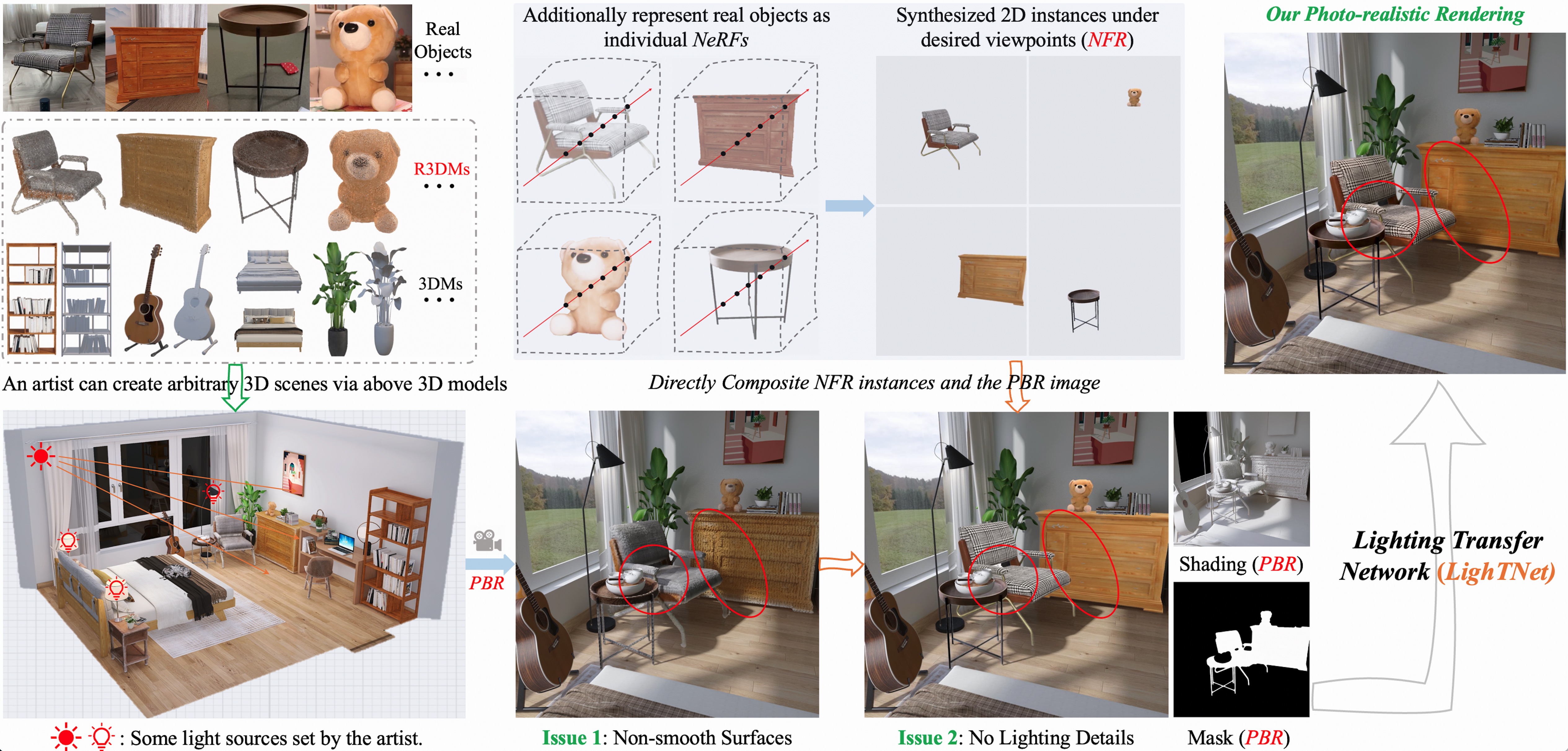
Figure 1: A Lighting Transfer Avenue. Left (Problem): Given some reconstructed rough 3D models (R3DMs) and designed 3D CAD models (3DMs), artists can use them to create any 3D scenes and freely perform arbitrary lighting simulation for each created scene. A physically-based rendering (PBR) system can only render low-quality images or videos for these scenes. Our goal is to render high-quality content from these possible scenes without training (or fitting) the newly created 3D scenes. Right (Solution): As an example, if we have pre-obtained a neural fields representation (e.g. NeRF [33]) for each real object, we can synthesize object instances for R3DMs in impressive quality through neural fields rendering (NFR). Unluckily, NFR instances cannot reflect the simulated lighting details (e.g., local shadows) on R3DMs. We propose a lighting transfer network (LighTNet) to bridge NFR and PBR, such that they can benefit from each other. In practice, LighTNet is trained once in a dataset and can be used for all the newly created 3D scenes with both seen and unseen R3DMs and arbitrary lighting (See “Generalizing to Real-Lighting” in Fig. 8).

In further, artists may perform free lighting simulation to their created 3D scenes (e.g. setting several strong light sources) to capture realistic renderings. The remained question is that the above rendering routing cannot reflect the simulated lighting details on R3DMs in PBR pipelines, especially when object interactions in the 3D scene creation cause local shadows. To solve the dilemma, we propose a Lighting Transfer Network (LighTNet) to bridge NFR and PBR, such that they can benefit from each other. LighTNet takes “Shading” rendered from a PBR system and a synthesized image by NFR techniques (e.g. NeRF) as input and outputs photo-realistic renderings with rich lighting details. Taking inspiration from the image composition process in V-Ray [9], we prudently reformulate it to remedy the non-smooth “Shading” surfaces caused by R3DMs as well as better preserve lighting details. Furthermore, we propose perceptual-motivated constraints to optimize LightNet and introduce a novel Lab Angle loss which can enhance the contrast between lighting strength and colors. To train LighTNet, we synthesize R3DMs by injecting random noises into 3DMs and use these $<$R3DM, 3DM$>$ pairs as the training data. Once LighTNet is learned on the training data, it can be used for arbitrary newly created 3D scenes with both seen and unseen R3DMs. Experiments show that LighTNet is superior in synthesizing impressive lighting details.

In summary, our main contributions are as follows:

• We present a lighting transfer avenue that allows artists to create arbitrary 3D scenes, flexibly simulate lighting, and freely render photo-realistic images and videos via R3DMs and 3DMs in any graphic software.

• We develop a lighting transfer network (LighTNet) leveraging a prudently reformulated image composition formulation. It can bridge the lighting gap between PBR and NFR, and is promising to remedy the non-smooth “Shading” surfaces caused by R3DMs.

• We introduce a Lab Angle loss to enhance the contrast between lighting strength and colors which can further improve the rendering quality.

2 Related Work

Typical SFM and MVS approches [2, 46, 47] can reconstruct 3D meshes of objects that are with rich textures in reasonable quality. Leveraging large database, researchers exploit deep neural networks to reconstruct point clouds [1, 14, 54, 62], voxel grids [8, 12, 16, 60, 59], and meshes [23, 25, 40, 56] from single or multiple images. Other works show learning implicit representations for objects is a promising avenue [3, 61, 45, 41, 32, 30, 57, 39, 63]. For example, IDR [64] and DVR [38] take advantage of differentiable rendering formulation for implicit shape and texture representations and show the possibility of recovering smooth surfaces for objects with rich textures from a set of posed images. They cannot handle many real-world cases, such as big items with flattened areas (e.g. furniture). Besides, they fall into the neural rendering category, thus would also benefit from the lighting transfer avenue. To the best of our knowledge, no high-performing solution can automatically reconstruct perfect meshes and their UV texture atlases for real-world objects. Moreover, even if we can obtain an ideal 3D model with a perfect topology, we also need to rebuild its UV textures and materials. Unfortunately, texture and material recovery are currently receiving relatively poor attention, and the progress is not smooth.

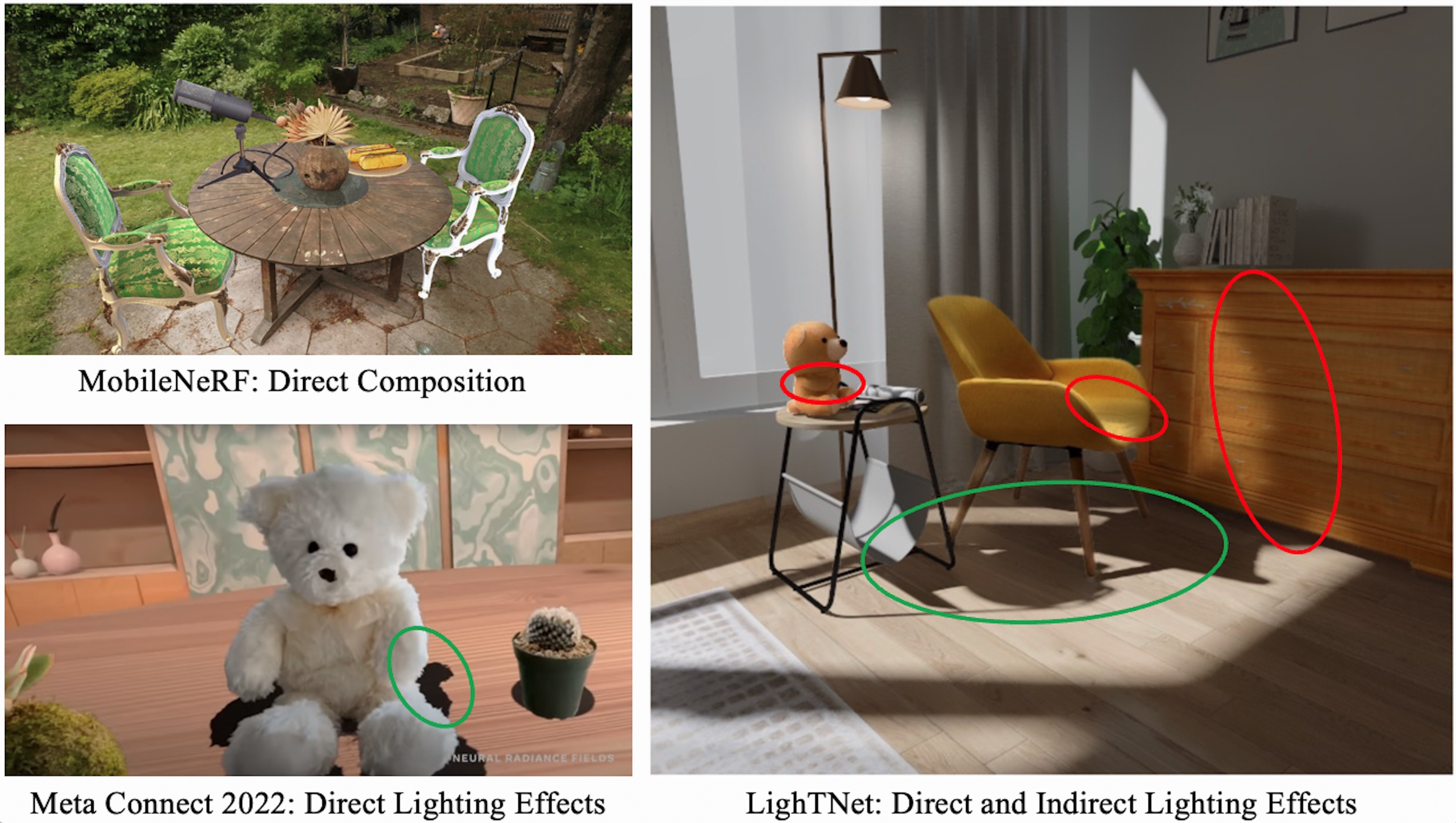
Figure 2: Compositing Individual NeRF Objects. Several concurrent works [11, 31] show it’s possible to represent real-world objects as individual NeRFs and R3DMs for freely 3D scene creation and rendering. LighTNet goes a futher step by considering the indirect lighting effects such as local shadows on R3DMs caused by objects interactions.

Recent advances show neural fields representations are promising to describe scenes, and support rendering photo-realistic images of the fitted scenes under desired viewpoints [33, 11, 29, 35, 37, 42, 44, 69, 51, 4, 66, 52, 10, 17, 5, 55]. Concurrently, MobileNeRF [11] has performed scene edition application by representing real-world objects as individual NeRFs and R3DMs. Meta in Meta Connect 2022 [31] demonstrates this routine supports direct shadow simulations. The proposed lighting transfer avenue goes a further step by modeling the indirect lighting effects, such as local shadows on R3DMs caused by object-to-object interactions. There are several works [43, 65, 53] that have also exploited free scene lighting editing. Unlike these approaches that would first perform per-scene optimization before editing and rendering, LighTNet is a generic solution that can be directly integrated into practical 3D modeling pipelines for scene creation and rendering without per-scene optimization. It’s worth mentioning that some works study inverse rendering with implicit neural representations that enable material editing and free view relighting of their reconstructed scenes (or objects) [68, 70, 7, 50, 72]. Our setting is totally different from theirs. For example, they can only synthesize local shadows caused by self-occlusion of its optimized single scene (or object). In fact, they have not considered compositing individual NeRFs to freely create and edit 3D scenes, thus have not handle the possible indirect lighting effects caused by objects interaction. We refer to the supplementary for more discussion about the differences.

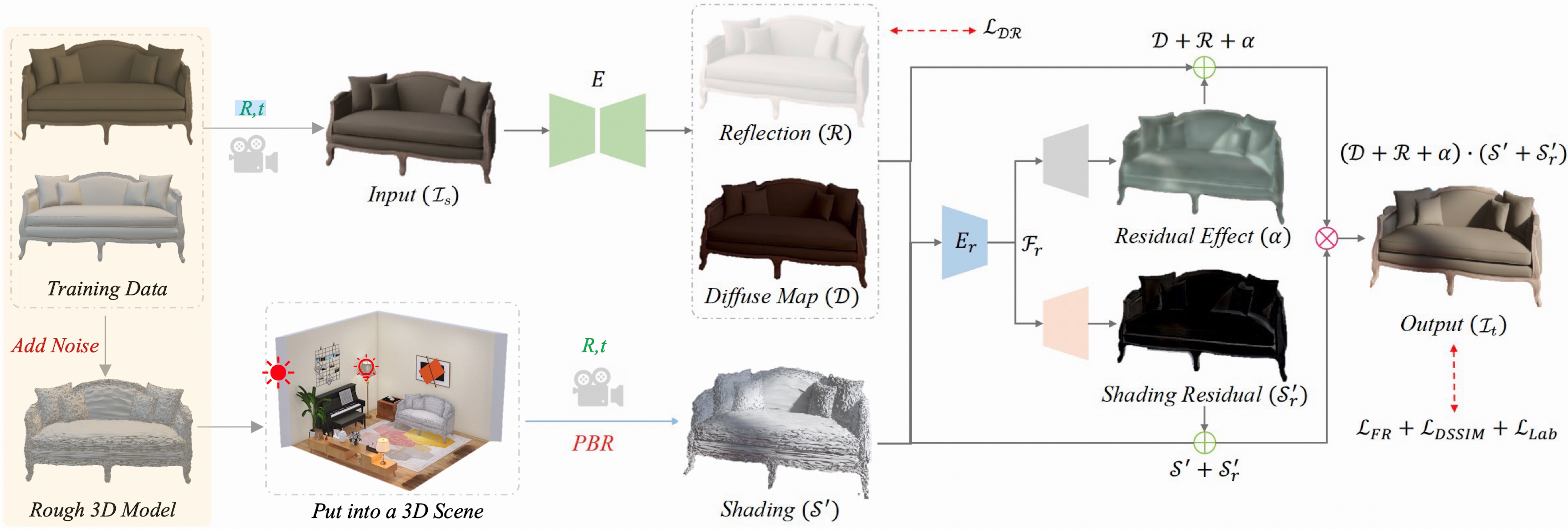
Figure 3: Training a LighTNet. LighTNet aims to transfer the lighting details from an imperfect shading map $\mathcal{S}^{\prime}$ to the corresponding image $\mathcal{I}_{s}$. It reasons about the reformulated image composition model $\mathcal{I}_{t}=(\mathcal{D}+\mathcal{R}+\alpha)\cdot(\mathcal{S}^{\prime}+\mathcal{S}^{\prime}_{r})$. The yellow (left) part shows the $<$R3DM, 3DM$>$ pairs generation process, and is only included in the training process. Once optimized, LighTNet can be used for any newly created 3D scenes with both seen and unseen R3DMs and support free lighting simulation. In the inference phase, $\mathcal{I}_{s}$ of an object is the 2D instance synthesized by a trained NeRF or any other high-performing free view synthesis formulations (See Fig. 1 and Fig. 4).

3 Lighting Transfer Network (LighTNet)

As shown in Fig. 3, the goal of LighTNet is to transfer the lighting details from an imperfect shading map $\mathcal{S}^{\prime}$ to the corresponding image $\mathcal{I}_{s}$. We will start with a brief introduction to the simplified image composition formulation in Sec. 3.1, which is the theoretical basis of LighTNet. Then, we explain the network architecture in Sec. 3.2. Finally, in Sec. 3.3, we introduce the proposed Lab Angle Loss and other involved objectives.

Importantly, in Sec. 4, we will take a specific example to explain the Lighting Transfer avenue. We show how a trained LighTNet allows us to flexibly create 3D scenes, edit lighting, and render high-quality images and videos via R3DMs and 3DMs.

3.1 Preliminaries: Image Composition

An image can be expressed as the point-wise product between its shading $\mathcal{S}$ and albedo $\mathcal{A}$, i.e., $\mathcal{I}=\mathcal{A}\cdot\mathcal{S}$, as discussed in [20, 28, 74, 26]. $\mathcal{A}$ is often simplified as a diffuse map which shows the base colors and textures used in materials with no lighting information. However, the render equation [22] in general physically-based renders tells us $\mathcal{A}$ should encode other material properties such as refraction and specularity. We follow the compositing process and definitions in V-Ray [9] and simplify its formulation as

$$\begin{split}\mathcal{I}=\mathcal{D}\cdot\mathcal{S}+\mathcal{R}\cdot\mathcal{R}_{l}+\alpha_{2},\end{split}$$ (1)

where $\mathcal{D}$ is the diffuse map, $\mathcal{S}$ is all the raw lighting (both direct and indirect ) in the scene and we regard it as “Shading” in this paper, $\mathcal{R}$ defines the strength of the reflection of the materials, $\mathcal{R}_{l}$ stores reflection information calculated from the materials’ reflection values in the scene, and $\alpha_{2}$ provides the interactive effects between other material properties and lighting. As $\mathcal{S}$ encodes the per-pixel lighting of a scene, we approximate $\mathcal{R}_{l}$ via $\mathcal{S}+\alpha_{1}$. Going a further step, we find that rendering the supervision information $\mathcal{S}+\alpha_{1}$ and $\alpha_{2}$ is impractical because we only have a rough geometry R3DM. Besides, learning them separately would increase our framework complexity. We thus further simplify the formulation as

$$\begin{split}\mathcal{I}=(\mathcal{D}+\mathcal{R}+\alpha)\cdot\mathcal{S}\end{split}$$ (2)

by regarding ${(R\cdot\alpha_{1}+\alpha_{2})}/{S}$ as a packed residual effect $\alpha$.

3.2 Architecture

Our lighting transfer network (LighTNet) is developed based on the formulation $\mathcal{I}=(\mathcal{D}+\mathcal{R}+\alpha)\cdot\mathcal{S}$. Given a training sample $(\mathcal{I}_{s},\mathcal{S}^{\prime},\bar{\mathcal{I}}_{t},\bar{\mathcal{D}},\bar{\mathcal{R}})$, where $\bar{\mathcal{I}}_{t}$, $\bar{\mathcal{D}}$, and $\bar{\mathcal{R}}$ are the ground-truth images, LighTNet takes $\mathcal{I}_{s}$ and $\mathcal{S}^{\prime}$ as inputs, and target at reconstructing $\bar{\mathcal{I}}_{t}$. See Sec. 5.1 for details about the training samples capturing process.

We utilize an encoder-decoder network $E$ to estimate both the diffuse map $\mathcal{D}$ and the reflection strength $\mathcal{R}$ from $\mathcal{I}_{s}$. We learn $\mathcal{R}$ and $\mathcal{D}$ in a supervised manner using:

$$\begin{split}\mathcal{L}_{\mathcal{D}\mathcal{R}}=|\mathcal{R}-\bar{\mathcal{R}}|+|\mathcal{D}-\bar{\mathcal{D}}|.\end{split}$$ (3)

After that, the remained major issue is that the shading $S^{\prime}$ is not smooth since its R3DM’s surfaces are uneven. We know that shading is determined by surface normal and illumination [74]. We clarify $\mathcal{D}$ and $\mathcal{R}$ mapping from $\mathcal{I}_{s}$ usually imply smooth normal information that could remedy $\mathcal{S}^{\prime}$. Towards the purpose, we obtain an intermediate representation by concatenating $\mathcal{S}^{\prime}$, $\mathcal{D}$, and $\mathcal{R}$ together, and take an encoder network ($E_{r}$) to map it to a feature $\mathcal{F}_{r}$. With $\mathcal{F}_{r}$, a straightforward option is to directly predict a smooth shading $\mathcal{S}$. In our experiments, we find a smoother $\mathcal{S}$ could be captured following $\mathcal{S}=\mathcal{S}^{\prime}+\mathcal{S}^{\prime}_{r}$, where $\mathcal{S}^{\prime}_{r}$ is the learned residual from $\mathcal{F}_{r}$ via a decoder network ($D_{\mathcal{S}^{\prime}}$).

Finally, as analyzed before, the model $\mathcal{I}=(\mathcal{D}+\mathcal{R})\cdot\mathcal{S}$ cannot describe the full lighting effects. Especially, our experiments in Fig. 6 show it cannot well preserve shadows. We thus follow Eqn. 2 to directly predict a residual effect $\alpha$ from $\mathcal{F}_{r}$ through another decoder network ($D_{\alpha}$). Considering all above, the target image can be composited as

$$\begin{split}\mathcal{I}_{t}=(\mathcal{D}+\mathcal{R}+\alpha)\cdot(\mathcal{S}^{\prime}+\mathcal{S}^{\prime}_{r}).\end{split}$$ (4)

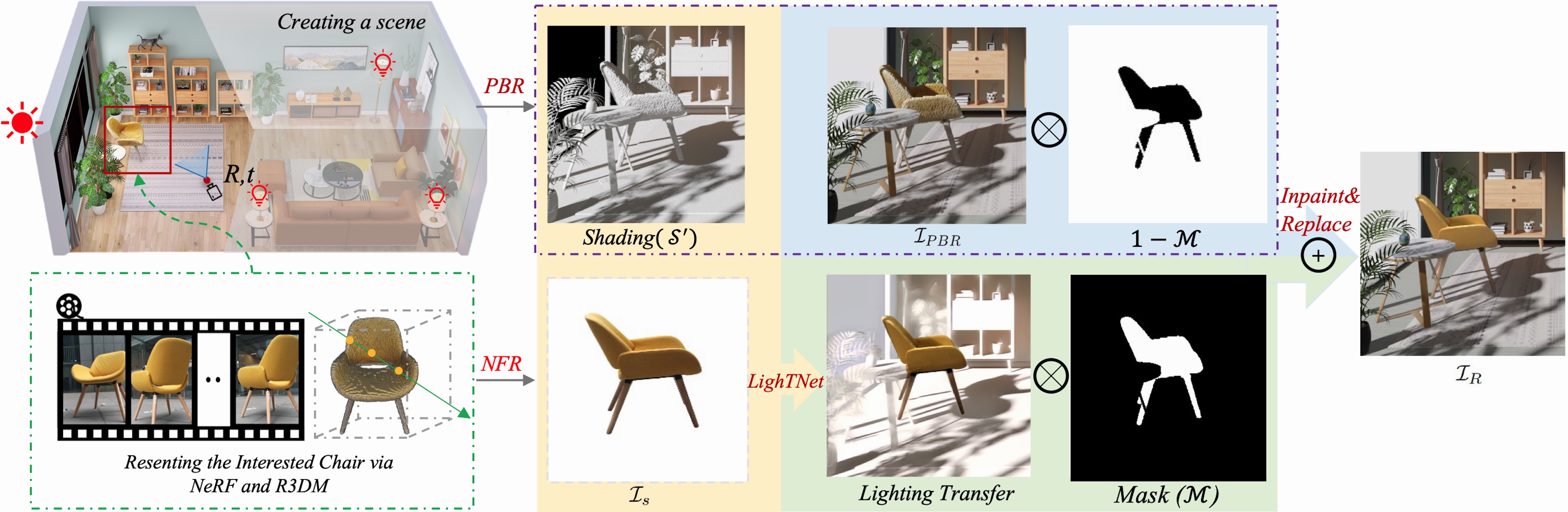
Figure 4: 3D Scene Creation and Rendering via R3DMs. We can represent real-world objects as individual NeRFs and R3DMs, and freely composite them to create unlimited 3D scenes. After lighting editing by artists, LighTNet can transfer direct and indirect lighting effects on R3DMs (e.g. $\mathcal{S}^{\prime}$) to the corresponding NFR instances (e.g. $\mathcal{I}_{s}$). See Sec. 4 for the detailed explanation.

3.3 Objectives

In previous relighting efforts, the L1 photometric loss $\mathcal{L}_{\emph{L1}}$ ($|\mathcal{I}_{t}-\bar{\mathcal{I}}_{t}|$ or $|\log\mathcal{I}_{t}-\log\bar{\mathcal{I}}_{t}|$) was commonly used as a major term to preserve the basic image content in the reconstruction process [48, 67, 24]. However, we find in our experiments it will degrade the lighting transfer ability of LighTNet as shown in Fig. 7. A possible reason is that it pushes the learning procedure to focus more on reducing the color differences instead of local lighting discrepancies. We thus propose to minimize the following losses that are closely related to perceptual quality and lighting effects.

Feature Reconstruction Loss. The feature reconstitution loss [21] encourages $\mathcal{I}_{t}$ to be perceptually similar to $\bar{\mathcal{I}}_{t}$ by matching their semantic features. We take VGG-19 [49] pretrained on ImageNet [13] as the feature extractor $\phi$ and denote $\phi_{j}(x)$ as the output of the $jth$ convolution block. The feature reconstruction loss is expressed as:

$$\begin{split}\mathcal{L}_{FR}=\frac{1}{C_{j}*H_{j}*W_{j}}\sum_{c,h,w}\|\phi_{j}(\mathcal{I}_{t})-\phi_{j}(\bar{\mathcal{I}}_{t})\|,\end{split}$$ (5)

where $C_{j}*H_{j}*W_{j}$ is the feature dimensions of $\phi_{j}(x)$. In this paper, we utilize activations of the third convolution block ($j=3$) to compute $\mathcal{L}_{FR}$.

Structural Dissimilarity. SSIM [58] is another perceptual-motivated metric that measures structural similarity between two images. We take the structural dissimilarity (DSSIM) as a measure following the success in [36]:

$$\begin{split}\mathcal{L}_{DSSIM}=\frac{1-\text{SSIM}(\mathcal{I}_{t},\bar{\mathcal{I}}_{t})}{2},\end{split}$$ (6)

Lab Angle Loss. We find that LighTNet optimized with aforementioned loss terms would produce images with darker global brightness as shown in Fig. 7. A possible reason is that $\mathcal{L}_{FR}$ and $\mathcal{L}_{DSSIM}$ only enhance local perceptual quality while overlooking the lighting contrast. In the paper, we thus propose a novel Lab Angle loss to consider the pixel-wise ratio between lighting strength and colors as:

$$\begin{split}\mathcal{L}_{Lab}=\frac{1}{H*W}\sum_{h,w}\arccos{(\frac{\langle\varphi(\mathcal{I}_{t})_{(h,w)},\varphi(\bar{\mathcal{I}}_{t})_{(h,w)}\rangle}{\|\langle\varphi(\mathcal{I}_{t})_{(h,w)},\varphi(\bar{\mathcal{I}}_{t})_{(h,w)}\rangle\|})},\end{split}$$ (7)

where $\langle x,y\rangle$ denotes the inner product of vector $x$ and $y$, $\varphi(\cdot)$ represents the RGB to Lab converter, $(h,w)$ is the spatial location, and $H*W$ is the image size.

Full Objective. Our LighTNet is optimized in an end-to-end fashion with the objective:

$$\begin{split}\mathcal{L}=\mathcal{L}_{\mathcal{D}\mathcal{R}}+\lambda_{1}\mathcal{L}_{FR}+\lambda_{2}\mathcal{L}_{DSSIM}+\lambda_{3}\mathcal{L}_{Lab},\end{split}$$ (8)

where the loss weights $\lambda_{1}$, $\lambda_{2}$, and $\lambda_{3}$, in all the experiments, are set to 0.05, 0.5, and 0.5, respectively.

4 Rendering with LighTNet and R3DMs

In this section, we show how a trained LighTNet and R3DMs can be flexibly integrated into practical 3D modeling workflows such as 3D scene creation and rendering. For example, we are interested in a real yellow chair, as shown in Fig. 4. Given its reconstructed R3DM and neural fields representation (NeRF [33] in this paper), we can create a 3D scene by putting the yellow chair’s R3DM and some 3DMs into a 3D room. Here, both the room and the involved 3DMs have not been seen before. To showcase the scene, we would like to render a high-quality image, in which the involved 3D models are with rich lighting details. Towards the goal, we can set a high-energy light source, and render a scene image $\mathcal{I}_{PBR}$, a shading $\mathcal{S}^{\prime}$, and an object’s mask $\mathcal{M}$, under a good viewpoint. Simultaneously, we synthesize an image $\mathcal{I}_{s}$ with the same camera pose via NeRF. Then, we are able to capture a target image $\mathcal{I}_{t}$ by transferring lighting from $\mathcal{S}^{\prime}\cdot\mathcal{M}$ to $\mathcal{I}_{s}\cdot\mathcal{M}$ via the trained LighTNet model. Finally, we replace $\mathcal{I}_{PBR}\cdot\mathcal{M}$ with $\mathcal{I}_{t}\cdot\mathcal{M}$ to obtain the final photo-realistic rendering $\mathcal{I}_{R}$. The complete process can be formulated as:

$$\begin{split}\mathcal{I}_{R}=\mathcal{I}_{PBR}\otimes(1-\mathcal{M})+\mathcal{M}\otimes\text{LighTNet}(\mathcal{I}_{s},\mathcal{S}^{\prime}),\end{split}$$ (9)

where $\otimes$ is the element-wise production operation. In practice, there will be some regions in boundary areas that cannot be covered by $\mathcal{I}_{t}$. We directly fill these regions via a SOTA image inpainting technique [34]. Some qualitative results are shown in Fig. 8.

5 Experiments

We conduct experiments to examine the lighting transfer avenue. More results are included in the supplementary.

5.1 Datasets

3DF-Lighting. Training Set: We take 50 3D scenes and the involved 30 3D CAD models (denoted as 3DMs) in 3D-FRONT [15] to construct the training set. First, we need to recover these objects’ rough 3D meshes (R3DMs). We simply adopt the mesh subdivision algorithm [27, 75] to densify the CAD models’ surfaces, then add random noise to each vertex. Second, for a specific object in a scene, we simulate uniform sunlight to the scene, randomly choose a viewpoint and render the object’s diffuse map $\bar{\mathcal{D}}$, reflection strength $\bar{\mathcal{R}}$, and color image $I_{s}$. Third, we randomly change the light source’s position and increase the lighting energy to capture a target image $\bar{\mathcal{I}}_{t}$. Finally, we render the rough shading $S^{\prime}$ by replacing the object’s 3DM as its R3DM. Following the pipeline, we can construct a training set $\{(\mathcal{I}_{s},\mathcal{S}^{\prime},\bar{\mathcal{I}}_{t},\bar{\mathcal{D}},\bar{\mathcal{R}}\}$. This paper takes Blender [6] with V-Ray plug-in as the render engine to secure these elements.

Evaluation Set: We build a test set using another 10 furniture shapes and 20 3D scenes from 3D-FRONT. We take one object as an example to present the test set building process. We randomly render 200 images from viewpoints sampled on a full sphere to learn its NeRF and R3DM. For each 3D scene, we put the object’s R3DM into the scene and randomly render thirty $\mathcal{S}^{\prime}$ and $\mathcal{M}$. Simultaneously, we synthesize the corresponding thirty $\mathcal{I}_{s}$ using its NeRF. Finally, we render the thirty $\bar{\mathcal{I}}_{t}$ (ground truth images) at size $800\times 800$ by replacing the R3DM with its 3DM. Each 3D scene’s light source and energy are pre-defined. Through the workflow, we construct a test set with 6,000 samples $\{(\mathcal{I}_{s},\mathcal{S}^{\prime},\bar{\mathcal{I}}_{t},\mathcal{M})\}$. We pre-assign V-Ray materials to each 3D model (R3DM and R3D) manually.

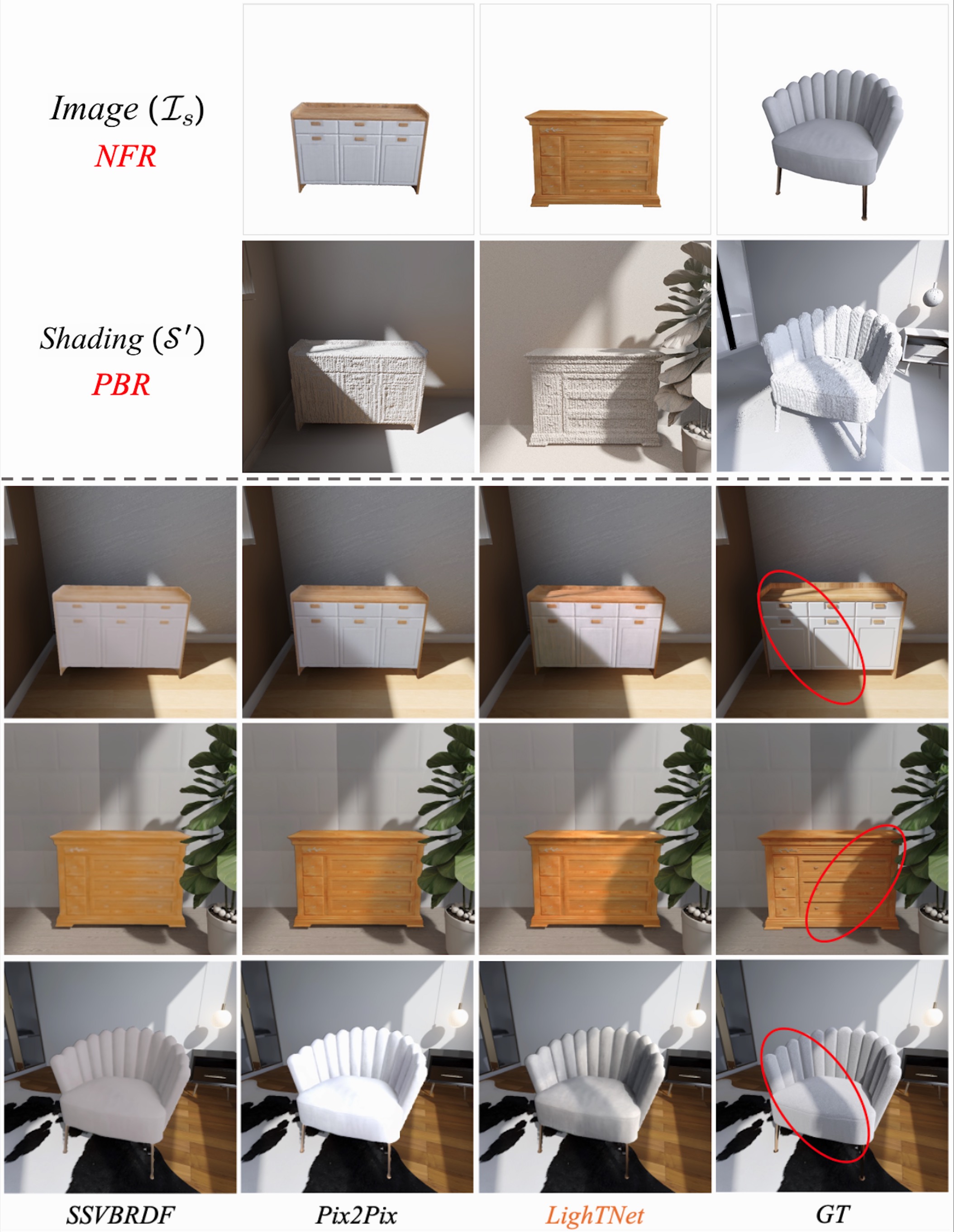
Figure 5: Qualitative Comparisons on 3DF-Lighting. We make qualitative comparisons with the reformulated Pix2Pix [19] and SSVBRDF [24]. LighTNet achieves realistic relighting results with impressive shadow details.

Generalizing to Real-Lighting. We also conduct qualitative evaluation on a real dataset named Real-Lighting. Specifically, we capture some object-centric videos via a mobile phone, and reconstruct these objects via NeRF. We create some 3D scenes using these objects’ R3DMs and other 3DMs . Some rendered images of these scenes are presented in Fig. 8. We can see the lighting details have been successfully preserved. The LighTNet model is trained only on the 3DF-Lighting train set. All the scenes and objects in Real-Lighting have not been seen previously.

5.2 Benchmark Comparisons

Building Baselines. We build baselines by reformulating three works, including Pix2Pix [19], DPR [73], and SSVBRDF [24], to study the lighting transfer setting. For Pix2Pix, we learn the mapping from $\mathcal{I}_{s}\oplus\mathcal{S}^{\prime}$ to $\mathcal{I}_{t}$, where $\oplus$ is the concatenate operation along the channel dimension. For DPR and SSVBRDF, we have not predicted the environment lighting (or spherical harmonics (SH)). Instead, we render the scenes’ SH lighting through PBR, and directly use it for the relighting process. All the methods (including LighTNet) have been trained on the 3DF-Lighting train set.

Performance. To measure the lighting synthesis ability, we take L1-Norm, PSNR, SSIM [58], and our Lab Angle loss as the metrics. From the scores presented in Table 1, our LighTNet outperforms the compared methods by a large margin. Especially, while the best PSNR and L1-Norm obtained by the baselines are 26.65 and 0.0345, LighTNet significantly improves them to 30.17 and 0.0219. It is not surprising since (1) DPR and SSVBRDF focus more on modeling global illumination, and (2) transferring lighting from shading with uneven surfaces is more challenging. Several qualitative comparisons are reported in Fig. 5. LighTNet achieves realistic relighting results with impressive shadow details. In Fig. 8, we illustrate some further examples of our approach generalizing to real objects, using the LighTNet model only trained on 3DF-Lighting.

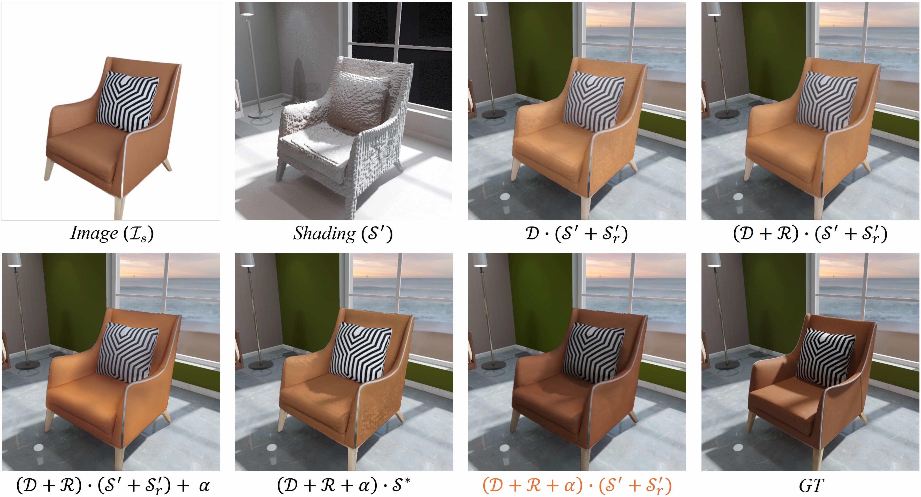
Figure 6: We qualitatively evaluate the lighting transfer ability of the image composition variants. $(\mathcal{D}+\mathcal{R}+\alpha)\cdot\mathcal{S}$ would be a much better choice for simulating the PBR compositing process.

Method	L1-Norm $\downarrow$	PSNR $\uparrow$	SSIM $\uparrow$	Lab Angle $\downarrow$
Pix2Pix [19]	0.0345	26.65	0.9042	0.4314
DPR[73]	0.0399	25.39	0.8692	0.4576
SSVBRDF [24]	0.0373	26.02	0.9040	0.3796
LighTNet	0.0219	30.17	0.9142	0.3137

Table 1: Quantitative Evaluation on 3DF-Lighting. We use the proposed Lab Angle distance and several widely studied metrics, including L1-Norm, PSNR, and SSIM[58], to measure a method’s lighting transfer ability. We reformulate these compared approaches to study our setting.

5.3 Ablation Studies

We argue that a slight numerical gain over the studied metrics may imply an improved visual experience since lighting is a detailed effect. We refer to the supplemental material for more qualitative comparisons.

Objectives. We discuss the objectives presented in Sec. 3.3 based on our lighting transfer formulation Eqn. 4. We take $\mathcal{L}_{FR}$ as the baseline, and incorporate other objectives one by one. $\mathcal{L}_{\mathcal{D}\mathcal{R}}$ is used in all the experiments. From Table 2, there is a remarkable gap between $\mathcal{L}_{L1}$ and $\mathcal{L}_{FR}$. Bringing in $\mathcal{L}_{DSSIM}$ yields a notable improvement over all the metrics. In further, although $\mathcal{L}_{Lab}$ only provides a slight PSNR gain ($+0.34$), it does enhance the lighting effects as reported in Fig. 7. It is worth mentioning that optimizing LighTNet with an auxiliary $\mathcal{L}_{L1}$ loss would largely degrade L1-Norm ($-0.021$) and PSNR ($-0.8$). See Fig. 7 for a qualitative evaluation.

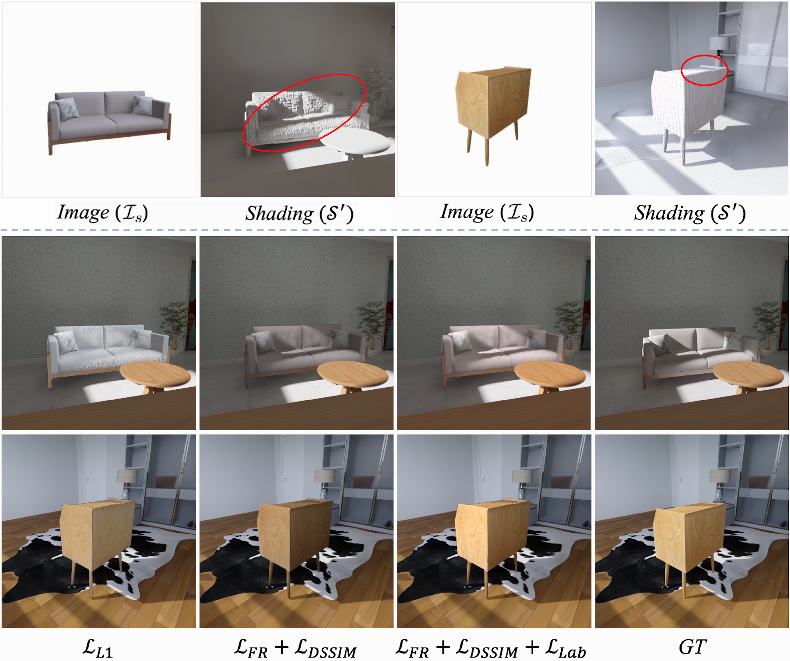
Figure 7: We qualitatively discuss the objectives in Sec. 3.3. $\mathcal{L}_{FR}+\mathcal{L}_{DSSIM}$ yields a notable improvement in dealing with uneven shading surface and local shadows compared to $\mathcal{L}_{L1}$. $\mathcal{L}_{Lab}$ could further enhance the lighting effects.

Image Composition Formulations. In Table 3 (Top), we study the image composition variants discussed in Sec. 3.1. Overall, our revised formulation $(\mathcal{D}+\mathcal{R}+\alpha)\cdot\mathcal{S}$ outperforms the baseline $\mathcal{D}\cdot\mathcal{S}$ by a significant margin. From the first three columns, while $\mathcal{R}$ supplements reflection effects, the residual $\alpha$ is important in encoding other lighting effects. By investigating $(\mathcal{D}+\mathcal{R}+\alpha)\cdot\mathcal{S}$ vs. $(\mathcal{D}+\mathcal{R})\cdot\mathcal{S}+\alpha$, we find that it would be much better to simulate the PBR compositing process following the product manner. Some qualitative comparisons are shown in Fig. 6.

Learning $S^{\prime}_{r}$ or Not? In Eqn. 4, we choose to learn a residual $S^{\prime}_{r}$ to remedy the uneven surfaces of $S^{\prime}$. There is an alternative that directly estimates a smooth shading $S^{*}$ from $\mathcal{F}_{r}$. As presented in Table 3 (Bottom), while $(\mathcal{D}+\mathcal{R}+\alpha)\cdot\mathcal{S}^{*}$ improves $(\mathcal{D}+\mathcal{R}+\alpha)\cdot\mathcal{S}^{\prime}$ by 0.65 on PSNR, our residual architecture significantly yields a PSNR gain of 1.47.

Objective				Metric
$\mathcal{L}_{FR}$	$\mathcal{L}_{DSSIM}$	$\mathcal{L}_{Lab}$	$\mathcal{L}_{L1}$	L1-Norm $\downarrow$	PSNR $\uparrow$	SSIM $\uparrow$	Lab Angle $\downarrow$
			$\surd$	0.0277	28.37	0.8774	0.3551
$\surd$				0.0254	29.06	0.9006	0.3717
$\surd$	$\surd$			0.0229	29.83	0.9129	0.3317
$\surd$	$\surd$	$\surd$		0.0219	30.17	0.9142	0.3137
$\surd$	$\surd$	$\surd$	$\surd$	0.0240	29.37	0.9102	0.3426

Table 2: We find that optimizing LighTNet with a L1 photometric loss ($\mathcal{L}_{L1}$ = $|\mathcal{I}_{t}-\bar{\mathcal{I}}_{t}|$) would yield a degenerate performance.

Variant	L1-Norm $\downarrow$	PSNR $\uparrow$	SSIM $\uparrow$	Lab Angle $\downarrow$
Composition Formulations ($\mathcal{S}=\mathcal{S}^{\prime}+\mathcal{S}^{\prime}_{r}$)
$\mathcal{D}\cdot\mathcal{S}$	0.0200083	28.46	0.9128	0.3449
$(\mathcal{D}+\mathcal{R})\cdot\mathcal{S}$	0.0262	28.83	0.9117	0.3411
$(\mathcal{D}+\mathcal{R})\cdot\mathcal{S}+\alpha$	0.0238	29.45	0.9040	0.3458
$(\mathcal{D}+\mathcal{R}+\alpha)\cdot\mathcal{S}$	0.0219	30.17	0.9142	0.3137
Architecture: Learning $\mathcal{S}^{\prime}_{r}$ or Not
$(\mathcal{D}+\mathcal{R}+\alpha)\cdot\mathcal{S}^{\prime}$	0.0260	28.70	0.8935	0.3574
$(\mathcal{D}+\mathcal{R}+\alpha)\cdot\mathcal{S}^{*}$	0.0241	29.35	0.8996	0.3473
$(\mathcal{D}+\mathcal{R}+\alpha)\cdot(\mathcal{S}^{\prime}+\mathcal{S}^{\prime}_{r})$	0.0219	30.17	0.9142	0.3137

Table 3: Image Composition Formulations. See Sec. 3.1 and Sec. 3.2 for explanations of these formulations. $\mathcal{S}^{*}$ means that we directly predict a smooth shading from $\mathcal{F}_{r}$ instead of estimating the shading residual $\mathcal{S}^{\prime}_{r}$.

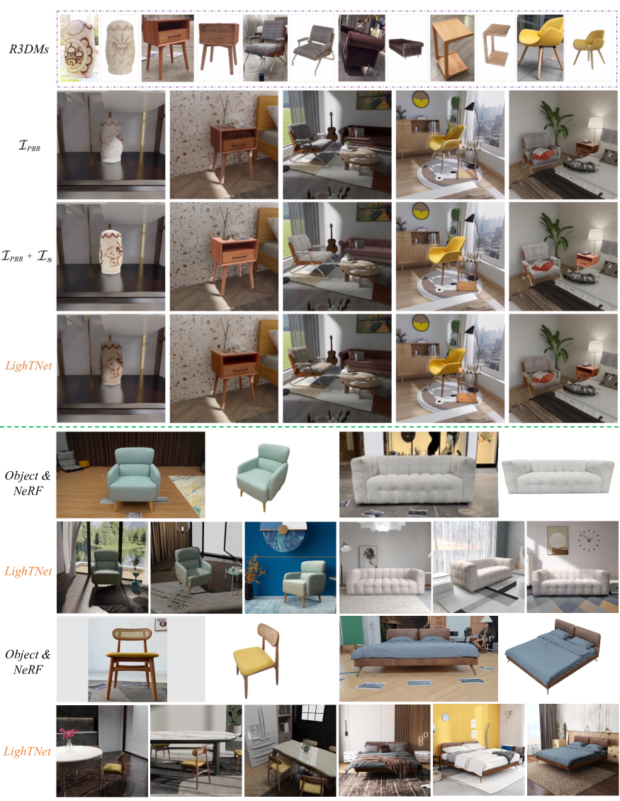
Figure 8: Generalizing to Real-Lighting. We reconstruct some real objects and use them to create some scenes. See Sec. 5.1 for an introduction. Bottom: We put the reconstructed objects to different 3D scenes. Here, NeRF means the 2D instance synthesized by NeRF. The lighting details have been successfully preserved by our LighTNet. Please see the shadows caused by object-to-object interactions. Note that, LighTNet here is only trained on the 3DF-Lighting training set. We refer to the supplementary for some rendered videos.

6 Conclusion

In this paper, we are prudent to rethink reconstructed rough 3D models (R3DMs) and present a lighting transfer avenue to flexibly integrate R3DMs into practical 3D modeling workflows such as 3D scene creation, lighting editing, and rendering. Physically-based rendering (PBR) would render low-quality images of scenes constructed by R3DMs. A remedy is to represent real-world objects as individual neural fields (e.g. NeRF) in addition to R3DMs, as neural fields rendering (NFR) can synthesize photo-realistic object images under desired viewpoints. The main question is that NFR instances cannot reflect the lighting details on R3DMs. We thus present a lighting transfer network (LighTNet) as a solution. LighTNet reasons about a reformulated image composition model and can bridge the lighting gaps between NFR and PBR, such that they can benefit from each other. Moreover, we introduce a new Lab angle loss to enhance the contrast between lighting strength and colors. Qualitative and quantitative comparisons show the superiority of LighTNet in preserving both direct and indirect lighting effects.

It is worth mentioning that NeRF in this paper is just a specific example to present the possibility of the lighting transfer avenue. In our method, the R3DM part is independent of the NFR synthesis (or NeRF) part. For a real object, we can utilize a method to reconstruct its R3DM, and use another method to perform 2D instance synthesizing if it enables better novel view synthesis than NeRF.

Supplementary Material

The supplementary materials consist of:

• A simple ablation on the impact of the smoothness of R3DMs on the final rendering quality.

• A discussion about the major limiation of LighTNet.

• An illustration of the training set construction process.

• A further explanation on the differences between LighTNet and some works that study inverse rending with implicit neural representation.

• The detailed network architectures.

• Importantly, a video that records that an artist designs some rooms via R3DMs and R3Ds and renders high-quality images or videos leveraging LighTNet.

• More qualitative results (images and videos).

S1 Ablation: Smoothness of R3DMs

We indicate again that NeRF [33] in this paper is just a specific example to present the possibility of the lighting transfer avenue. In our method, the R3DM part is independent of the NFR rendering part. For a real object, we can utilize an algorithm to reconstruct its R3DM, and use a different approach to perform 2D instance synthesizing. In S.Fig. S1, we explore the impact of the smoothness of R3DMs on the final rendering quality. For the “extremely noisy surfaces” case, LighTNet fails to render the lighting details and cannot address the uneven artifacts. The reasons are: (1) a PBR system cannot produce a correct shading map for extremely noisy meshes, as the lighting effects are closely related to surface normals; (2) The capability of LighTNet is not sufficient to remedy these very worse typologies.

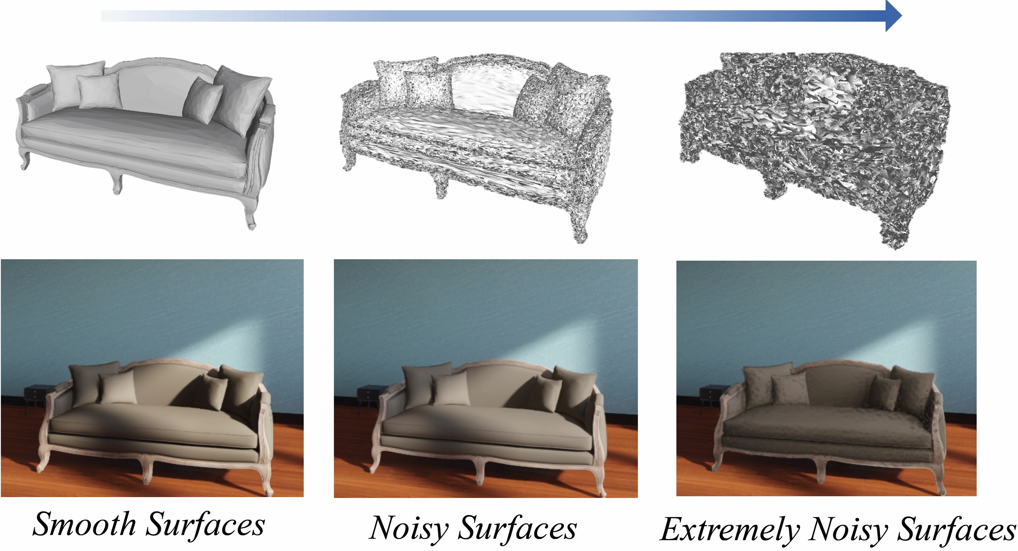
Figure S1: Smoothness of R3DMs. We simulate different levels of noises to the sofa’s 3D CAD model. It is not supersizing that: (1) If a method can recover smoother surfaces, LighTNet would perform better; and (2) LighTNet is not robust to extremely noisy meshes yet.

S2 Limitations

LighTNet cannot handle strong specular materials yet. As shown in S.Fig. S3, the synthesized 2D instances by NeRF contain the reflected content. It’s unavoidable yet as NeRF series learn to fit a captured scene for its free view synthesis. We find LighTNet would preserve the reflected content while ignoring the real reflected content of the newly created scenes. It should be one of the major limitations. This issue would disappear if future NeRF research or other view synthesis works can disentangle the reflected content from the objects’ textures.

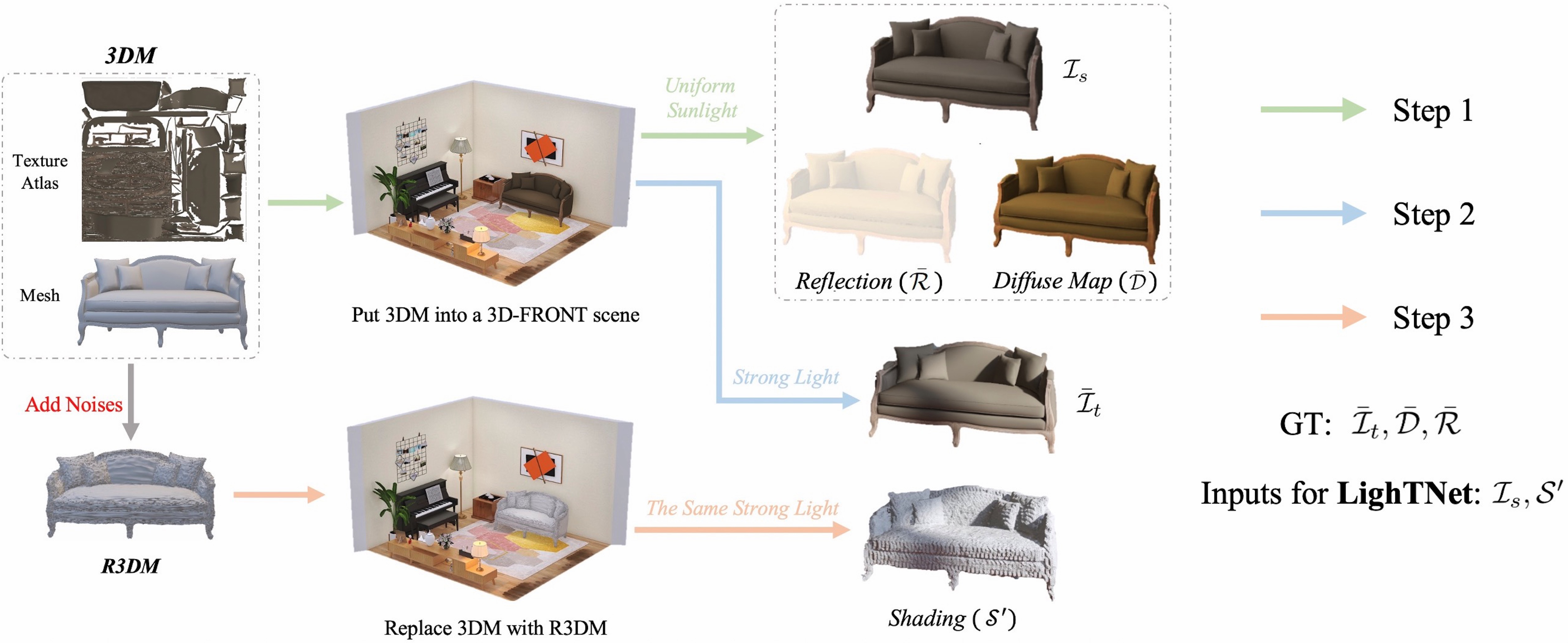
Figure S2: Training Set Construction. We take the “Sofa” case as an example to show how to capture a training sample $\{(\mathcal{I}_{s},\mathcal{S}^{\prime},\bar{\mathcal{I}}_{t},\bar{\mathcal{D}},\bar{\mathcal{R}}\}$ via 3D CAD models and 3D scenes. The elements are rendered by Blender[6]. LighTNet is trained once on the 3DF-Lighting training set, and can be used for all the newly created scenes with both seen and unseen R3DMs and arbitrary lighting.

S3 Training Set Construction

We have introduced the 3DF-Lighting training set construction process in Sec. 3.2 in the main paper. Here, we visualize a training sample capturing process in S.Fig. S2.

Quoted Texts: We take 50 3D scenes and the involved 30 3D CAD models (denoted as 3DMs) in 3D-FRONT [15] to construct the training set. First, we need to recover these objects’ rough 3D meshes (R3DMs). We simply adopt the mesh subdivision algorithm [27, 75] to densify the CAD models’ surfaces, then add random noise to each vertex. Second, for a specific object in a scene, we simulate uniform sunlight to the scene, randomly choose a viewpoint and render the object’s diffuse map $\bar{\mathcal{D}}$, reflection strength $\bar{\mathcal{R}}$, and color image $I_{s}$. Third, we randomly change the light source’s position and increase the lighting energy to capture a target image $\bar{\mathcal{I}}_{t}$. Finally, we render the rough shading $S^{\prime}$ by replacing the object’s 3DM as its R3DM. Following the pipeline, we can construct a training set $\{(\mathcal{I}_{s},\mathcal{S}^{\prime},\bar{\mathcal{I}}_{t},\bar{\mathcal{D}},\bar{\mathcal{R}}\}$. This paper takes Blender [6] with V-Ray plug-in as the render engine to secure these elements.

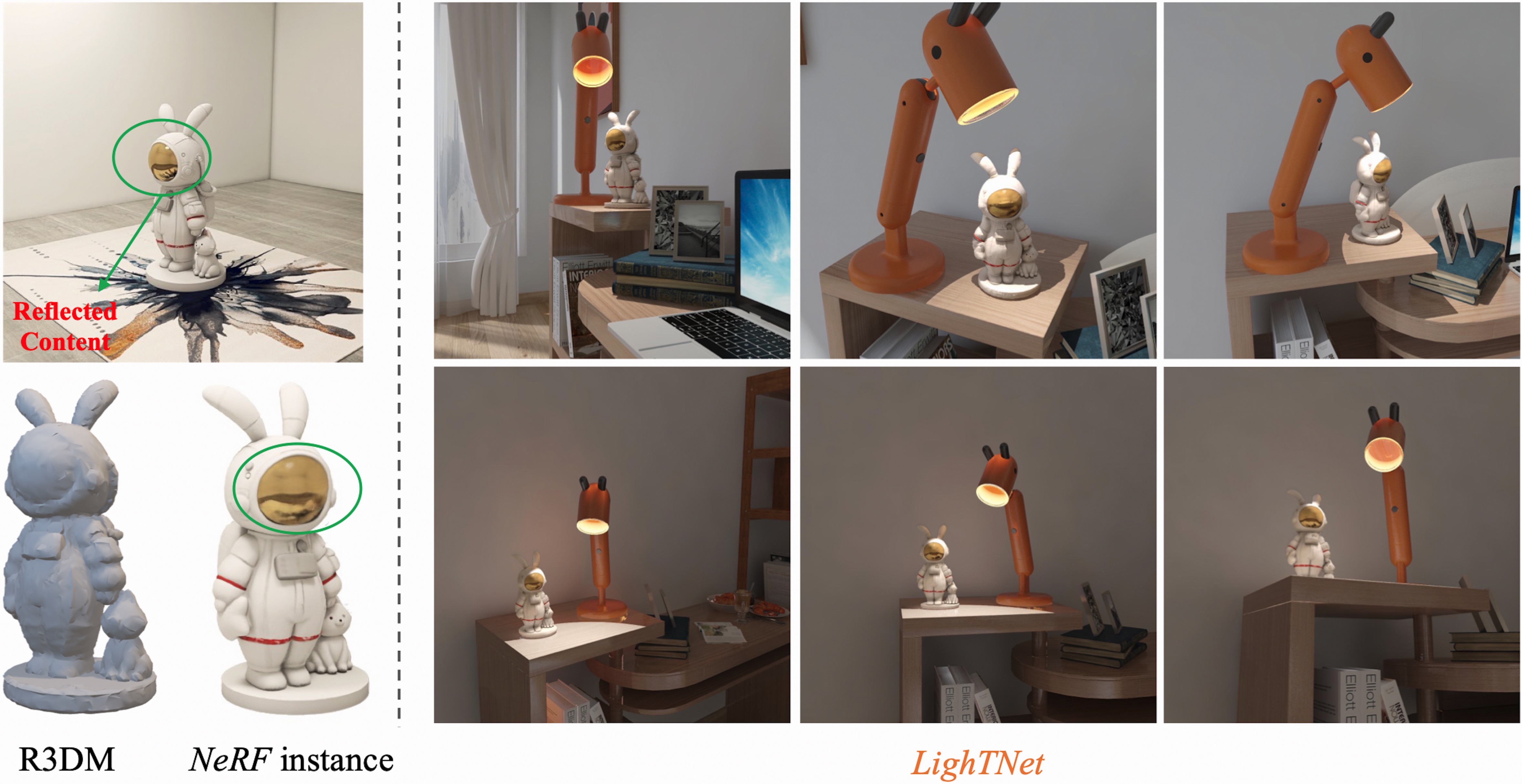
Figure S3: Failure Case. One of the major limitations of LighTNet is it cannot handle strong specular materials. See Sec. LABEL:sec:limitation for an explanation. Zoom in for a better view.

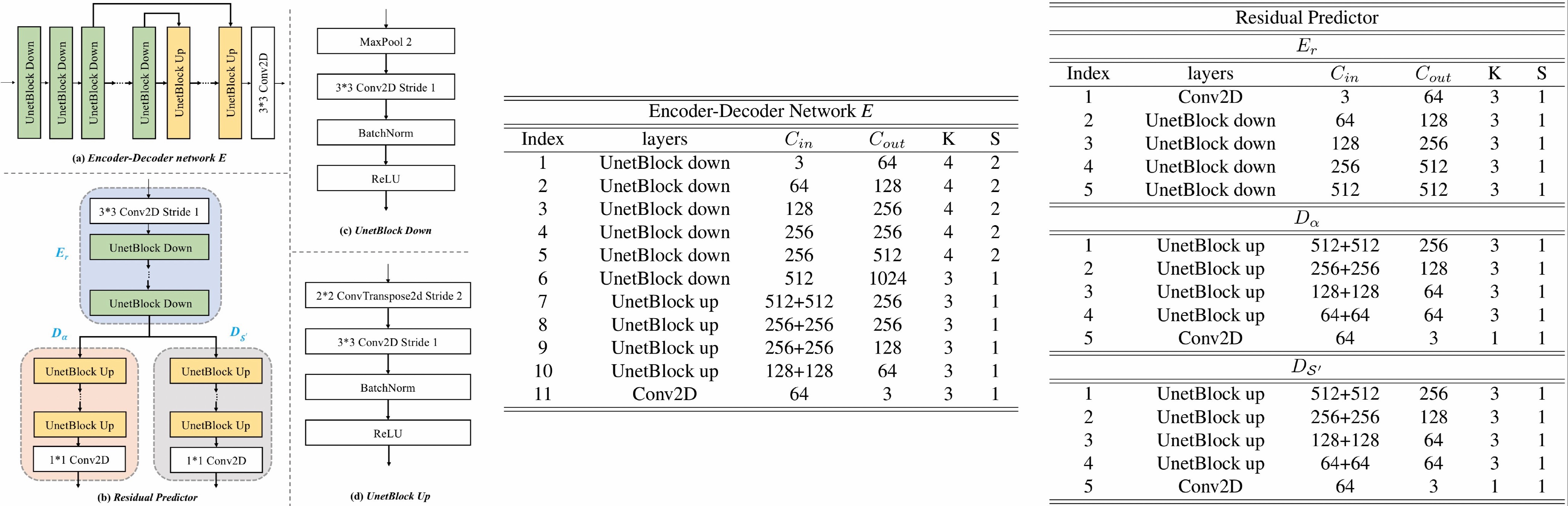
Figure S4: Network Architecture. (a). Encoder-Decoder Network E. (b). Residual Predictor. $D_{\alpha}$ and $D_{\mathcal{S}^{\prime}}$ share the same encoder $E_{r}$, and are used to estimate the residual lighting effect $\alpha$ and shading $\mathcal{S}^{\prime}$, respectively. (c). The U-Net downsampling block in E and $E_{r}$. (d). The U-Net upsampling block in E, $D_{\alpha}$ and $D_{\mathcal{S}^{\prime}}$. Zoom in for a better view.

S4 Relation to Inverse Rending with Implicit Neural Representation

Leveraging implicit neural representation, recent inverse rendering works can decompose a scene under complex and unknown illumination into spatially varying BRDF material properties [68, 70, 7, 50, 72]. These techniques enable material editing and free view relighting of the reconstructed scene. Here, we take NeRFactor [71] as an example to discuss the main differences of these works and the raised lighting transfer avenue. First, NeRFactor focused on estimate SVBRDF properties of single scene or object. Beyond free-view relighting, we can imagine that NeRFactor supports the object inserting application, i.e., inserting a 3D object into a static image, as we can extract the global lighting probes from the target static image. But if we would like to insert multiple 3D objects into a single image, NeRFactor would overlook the possible indirect lighting effects caused by object-to-object occlusion because there is no a “3D scene” concept involved. It’s worth mentioning NeRFactor can simulate local shadows caused by self-occlusion of its reconstructed single object. In contrast, we study a more practical problem that is “can we use rough 3D models, together with 3D CAD models drawing by artists, to create arbitrary 3D scenes and render high-quality contents?”. Thereby, our studied setting is totally different from the setting of NeRFactor. Second, in the proposed lighting transfer avenue, the R3DM part is independent with the NFR synthesis part. For a real object, we can use a method to reconstruct its R3DM, and use another method to perform 2D instance synthesizing. This paper takes NeRF as an example to explain the proposed avenue because: (1) it supports high-quality novel view synthesis; and (2) at the same time, we can conveniently extract a R3DM from a trained NeRF via a marching cube algorithm. From this perspective, we can apply NeRFactor instead of NeRF for 2D instance synthesizing. But as analyzed before, how should we handle the indirect lighting details caused by the interaction of multiple 3D objects? The introduced LighTNet could give a possible answer to this question.

S5 Network Architectures

The network architectures for the lighting transfer network (LighTNet) are reported in S.Figure S4. For convenience, we use the following abbreviation: $C_{in}$ = Input Channel, $C_{out}$ = Feature Channel, K = Kernel Size, S = Stride Size, Conv2D = Convolutional Layer.

S6 More Qualitative Results

S.Figure S5 provides more qualitative comparisons on the 3DF-Lighting test set. In S.Figure S6-S8 and the supplemental video, we incorporate more rendered results of scenes created by R3DMs of real objects (See ”Generalizing to Real-Lighting” in the main paper).

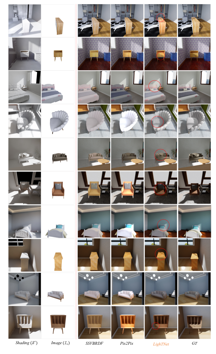
Figure S5: More qualitative comparisons with baseline methods on the 3DF-Lighting test set. LighTNet can well preserve the lighting details (e.g., local shadows.) Zoom in for a better view.

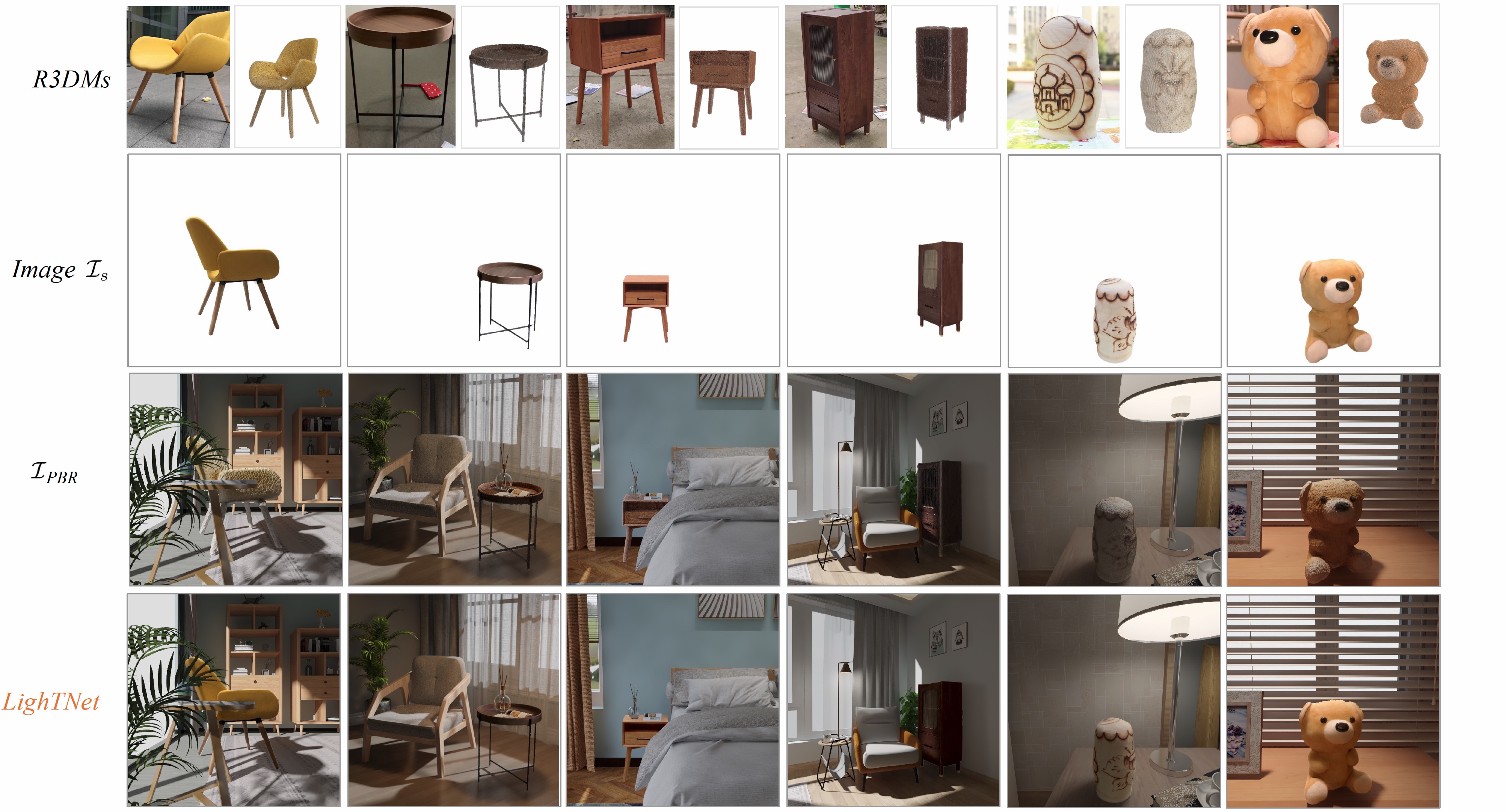
Figure S6: More rendered results of scenes created by R3DMs of real objects. Zoom in for a better view.

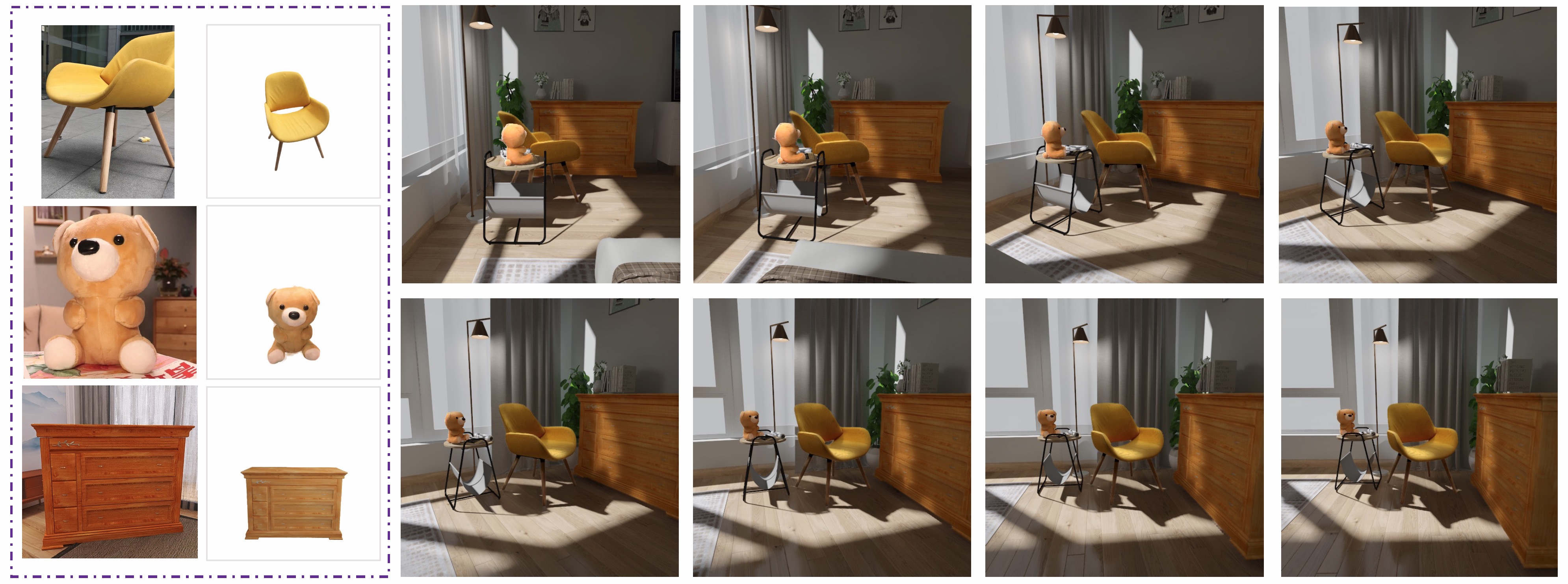
Figure S7: The R3DMs including bear, chair, and cabinet are put into room to make it collaborate with other 3D CAD furniture. Their lightings are transferred by LighTNet, while other 3D CAD models are rendered by PBR. We can see that R3DMs transferred by LighTNet can be well compatible with the PBR scene. Zoom in for a better view.

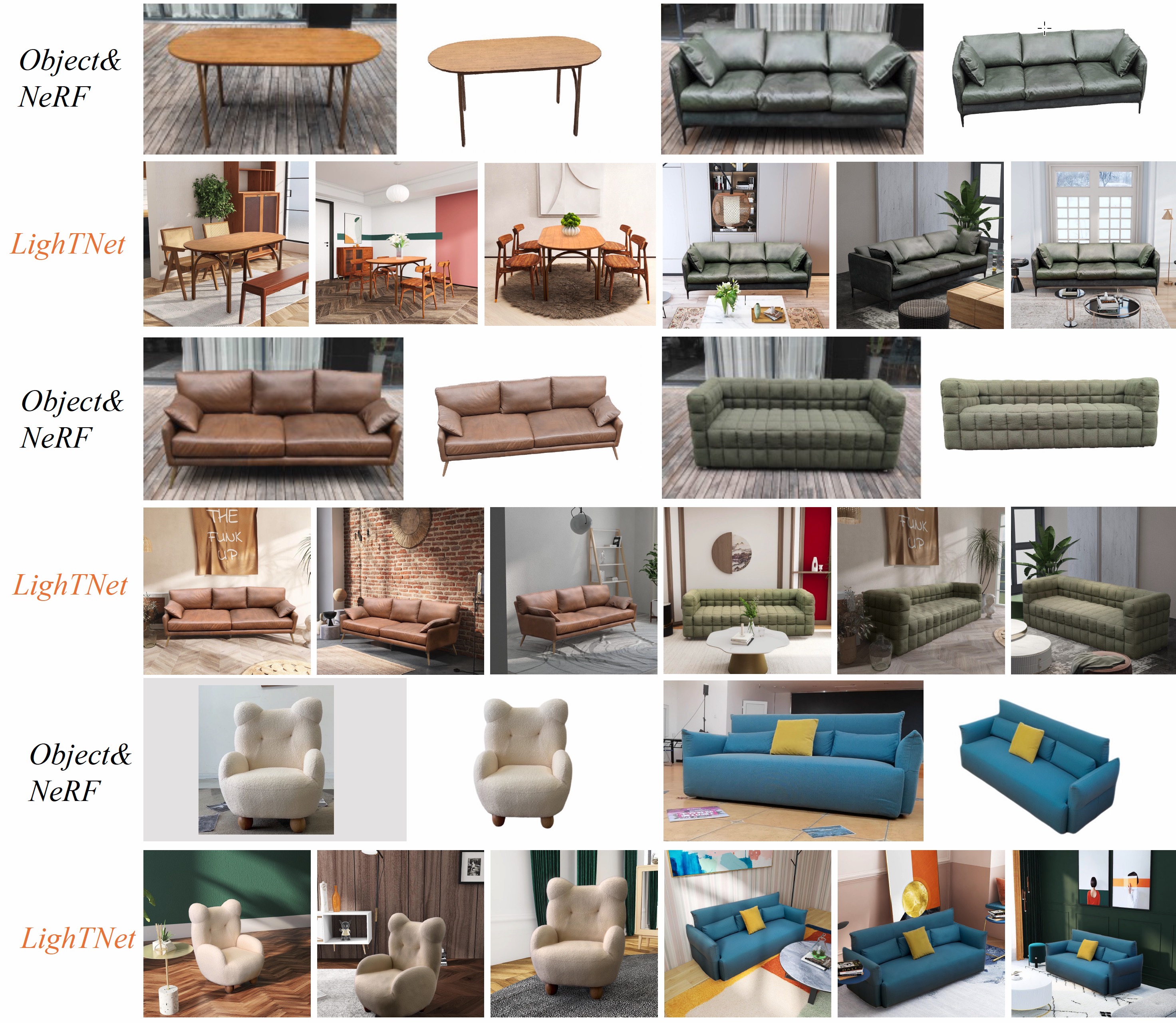
Figure S8: We put the reconstructed objects to different 3D scenes. Here, NeRF means the 2D instance synthesized by NeRF. The lighting details have been successfully preserved by our LighTNet approach.

References

- [1] Panos Achlioptas, Olga Diamanti, Ioannis Mitliagkas, and Leonidas Guibas. Learning representations and generative models for 3d point clouds. In International conference on machine learning, pages 40–49. PMLR, 2018.
- [2] Alex M Andrew. Multiple view geometry in computer vision. Kybernetes, 2001.
- [3] Matan Atzmon, Niv Haim, Lior Yariv, Ofer Israelov, Haggai Maron, and Yaron Lipman. Controlling neural level sets. arXiv preprint arXiv:1905.11911, 2019.
- [4] Jonathan T. Barron, Ben Mildenhall, Matthew Tancik, Peter Hedman, Ricardo Martin-Brualla, and Pratul P. Srinivasan. Mip-nerf: A multiscale representation for anti-aliasing neural radiance fields. In Proceedings of the IEEE/CVF International Conference on Computer Vision (ICCV), pages 5855–5864, October 2021.
- [5] Jonathan T. Barron, Ben Mildenhall, Dor Verbin, Pratul P. Srinivasan, and Peter Hedman. Mip-nerf 360: Unbounded anti-aliased neural radiance fields. In Proceedings of the IEEE/CVF Conference on Computer Vision and Pattern Recognition (CVPR), pages 5470–5479, June 2022.
- [6] Blender. https://www.blender.org.
- [7] Mark Boss, Raphael Braun, Varun Jampani, Jonathan T Barron, Ce Liu, and Hendrik Lensch. Nerd: Neural reflectance decomposition from image collections. arXiv preprint arXiv:2012.03918, 2020.
- [8] Andrew Brock, Theodore Lim, James M Ritchie, and Nick Weston. Generative and discriminative voxel modeling with convolutional neural networks. arXiv preprint arXiv:1608.04236, 2016.
- [9] Chaosgroup. V-ray render elements. https://docs.chaos.com/display/VMAX/RGB_Color.
- [10] Anpei Chen, Zexiang Xu, Andreas Geiger, Jingyi Yu, and Hao Su. Tensorf: Tensorial radiance fields. In European Conference on Computer Vision (ECCV), 2022.
- [11] Zhiqin Chen, Thomas Funkhouser, Peter Hedman, and Andrea Tagliasacchi. Mobilenerf: Exploiting the polygon rasterization pipeline for efficient neural field rendering on mobile architectures. arXiv preprint arXiv:2208.00277, 2022.
- [12] Christopher B Choy, Danfei Xu, JunYoung Gwak, Kevin Chen, and Silvio Savarese. 3d-r2n2: A unified approach for single and multi-view 3d object reconstruction. In European conference on computer vision, pages 628–644. Springer, 2016.
- [13] Jia Deng, Wei Dong, Richard Socher, Li-Jia Li, Kai Li, and Li Fei-Fei. Imagenet: A large-scale hierarchical image database. In 2009 IEEE conference on computer vision and pattern recognition, pages 248–255. Ieee, 2009.
- [14] Haoqiang Fan, Hao Su, and Leonidas J Guibas. A point set generation network for 3d object reconstruction from a single image. In Proceedings of the IEEE conference on computer vision and pattern recognition, pages 605–613, 2017.
- [15] Huan Fu, Bowen Cai, Lin Gao, Ling-Xiao Zhang, Jiaming Wang, Cao Li, Qixun Zeng, Chengyue Sun, Rongfei Jia, Binqiang Zhao, et al. 3d-front: 3d furnished rooms with layouts and semantics. In Proceedings of the IEEE/CVF International Conference on Computer Vision, pages 10933–10942, 2021.
- [16] Matheus Gadelha, Subhransu Maji, and Rui Wang. 3d shape induction from 2d views of multiple objects. In 2017 International Conference on 3D Vision (3DV), pages 402–411. IEEE, 2017.
- [17] Tao Hu, Shu Liu, Yilun Chen, Tiancheng Shen, and Jiaya Jia. Efficientnerf efficient neural radiance fields. In Proceedings of the IEEE/CVF Conference on Computer Vision and Pattern Recognition (CVPR), pages 12902–12911, June 2022.
- [18] Po-Han Huang, Kevin Matzen, Johannes Kopf, Narendra Ahuja, and Jia-Bin Huang. Deepmvs: Learning multi-view stereopsis. In Proceedings of the IEEE Conference on Computer Vision and Pattern Recognition, pages 2821–2830, 2018.
- [19] Phillip Isola, Jun-Yan Zhu, Tinghui Zhou, and Alexei A Efros. Image-to-image translation with conditional adversarial networks. In Proceedings of the IEEE conference on computer vision and pattern recognition, pages 1125–1134, 2017.
- [20] Michael Janner, Jiajun Wu, Tejas D Kulkarni, Ilker Yildirim, and Joshua B Tenenbaum. Self-supervised intrinsic image decomposition. In Proceedings of the 31st International Conference on Neural Information Processing Systems, pages 5938–5948, 2017.
- [21] Justin Johnson, Alexandre Alahi, and Li Fei-Fei. Perceptual losses for real-time style transfer and super-resolution. In European conference on computer vision, pages 694–711. Springer, 2016.
- [22] James T Kajiya. The rendering equation. In Proceedings of the 13th annual conference on Computer graphics and interactive techniques, pages 143–150, 1986.
- [23] Angjoo Kanazawa, Shubham Tulsiani, Alexei A Efros, and Jitendra Malik. Learning category-specific mesh reconstruction from image collections. In Proceedings of the European Conference on Computer Vision (ECCV), pages 371–386, 2018.
- [24] Zhengqin Li, Zexiang Xu, Ravi Ramamoorthi, Kalyan Sunkavalli, and Manmohan Chandraker. Learning to reconstruct shape and spatially-varying reflectance from a single image. ACM Transactions on Graphics (TOG), 37(6):1–11, 2018.
- [25] Yiyi Liao, Simon Donne, and Andreas Geiger. Deep marching cubes: Learning explicit surface representations. In Proceedings of the IEEE Conference on Computer Vision and Pattern Recognition, pages 2916–2925, 2018.
- [26] Yunfei Liu, Yu Li, Shaodi You, and Feng Lu. Unsupervised learning for intrinsic image decomposition from a single image. In Proceedings of the IEEE/CVF Conference on Computer Vision and Pattern Recognition, pages 3248–3257, 2020.
- [27] C. Loop. Smooth subdivision surfaces based on triangles. Master’s thesis, Department of Mathematics, University of Utah, 1987.
- [28] Wei-Chiu Ma, Hang Chu, Bolei Zhou, Raquel Urtasun, and Antonio Torralba. Single image intrinsic decomposition without a single intrinsic image. In Proceedings of the European Conference on Computer Vision (ECCV), pages 201–217, 2018.
- [29] Ricardo Martin-Brualla, Noha Radwan, Mehdi SM Sajjadi, Jonathan T Barron, Alexey Dosovitskiy, and Daniel Duckworth. Nerf in the wild: Neural radiance fields for unconstrained photo collections. In Proceedings of the IEEE/CVF Conference on Computer Vision and Pattern Recognition, pages 7210–7219, 2021.
- [30] Lars Mescheder, Michael Oechsle, Michael Niemeyer, Sebastian Nowozin, and Andreas Geiger. Occupancy networks: Learning 3d reconstruction in function space. In Proceedings of the IEEE/CVF Conference on Computer Vision and Pattern Recognition, pages 4460–4470, 2019.
- [31] Meta. Meta connect 2022. https://www.youtube.com/watch?v=hvfV-iGwYX8.
- [32] Mateusz Michalkiewicz, Jhony K Pontes, Dominic Jack, Mahsa Baktashmotlagh, and Anders Eriksson. Implicit surface representations as layers in neural networks. In Proceedings of the IEEE/CVF International Conference on Computer Vision, pages 4743–4752, 2019.
- [33] Ben Mildenhall, Pratul P Srinivasan, Matthew Tancik, Jonathan T Barron, Ravi Ramamoorthi, and Ren Ng. Nerf: Representing scenes as neural radiance fields for view synthesis. In European Conference on Computer Vision, pages 405–421. Springer, 2020.
- [34] Kamyar Nazeri, Eric Ng, Tony Joseph, Faisal Z Qureshi, and Mehran Ebrahimi. Edgeconnect: Generative image inpainting with adversarial edge learning. arXiv preprint arXiv:1901.00212, 2019.
- [35] Thomas Neff, Pascal Stadlbauer, Mathias Parger, Andreas Kurz, Chakravarty R Alla Chaitanya, Anton Kaplanyan, and Markus Steinberger. Donerf: Towards real-time rendering of neural radiance fields using depth oracle networks. arXiv preprint arXiv:2103.03231, 2021.
- [36] Thomas Nestmeyer, Jean-François Lalonde, Iain Matthews, and Andreas Lehrmann. Learning physics-guided face relighting under directional light. In Proceedings of the IEEE/CVF Conference on Computer Vision and Pattern Recognition, pages 5124–5133, 2020.
- [37] Michael Niemeyer and Andreas Geiger. Giraffe: Representing scenes as compositional generative neural feature fields. arXiv preprint arXiv:2011.12100, 2020.
- [38] Michael Niemeyer, Lars Mescheder, Michael Oechsle, and Andreas Geiger. Differentiable volumetric rendering: Learning implicit 3d representations without 3d supervision. In Proceedings of the IEEE/CVF Conference on Computer Vision and Pattern Recognition, pages 3504–3515, 2020.
- [39] Michael Oechsle, Songyou Peng, and Andreas Geiger. Unisurf: Unifying neural implicit surfaces and radiance fields for multi-view reconstruction. In Proceedings of the IEEE/CVF International Conference on Computer Vision, pages 5589–5599, 2021.
- [40] Junyi Pan, Xiaoguang Han, Weikai Chen, Jiapeng Tang, and Kui Jia. Deep mesh reconstruction from single rgb images via topology modification networks. In Proceedings of the IEEE/CVF International Conference on Computer Vision, pages 9964–9973, 2019.
- [41] Jeong Joon Park, Peter Florence, Julian Straub, Richard Newcombe, and Steven Lovegrove. Deepsdf: Learning continuous signed distance functions for shape representation. In Proceedings of the IEEE/CVF Conference on Computer Vision and Pattern Recognition, pages 165–174, 2019.
- [42] Sida Peng, Yuanqing Zhang, Yinghao Xu, Qianqian Wang, Qing Shuai, Hujun Bao, and Xiaowei Zhou. Neural body: Implicit neural representations with structured latent codes for novel view synthesis of dynamic humans. In Proceedings of the IEEE/CVF Conference on Computer Vision and Pattern Recognition, pages 9054–9063, 2021.
- [43] Julien Philip, Sébastien Morgenthaler, Michaël Gharbi, and George Drettakis. Free-viewpoint indoor neural relighting from multi-view stereo. ACM Transactions on Graphics (TOG), 40(5):1–18, 2021.
- [44] Albert Pumarola, Enric Corona, Gerard Pons-Moll, and Francesc Moreno-Noguer. D-nerf: Neural radiance fields for dynamic scenes. arXiv preprint arXiv:2011.13961, 2020.
- [45] Shunsuke Saito, Zeng Huang, Ryota Natsume, Shigeo Morishima, Angjoo Kanazawa, and Hao Li. Pifu: Pixel-aligned implicit function for high-resolution clothed human digitization. In Proceedings of the IEEE/CVF International Conference on Computer Vision, pages 2304–2314, 2019.
- [46] Johannes Lutz Schönberger and Jan-Michael Frahm. Structure-from-motion revisited. In Conference on Computer Vision and Pattern Recognition (CVPR), 2016.
- [47] Johannes Lutz Schönberger, Enliang Zheng, Marc Pollefeys, and Jan-Michael Frahm. Pixelwise view selection for unstructured multi-view stereo. In European Conference on Computer Vision (ECCV), 2016.
- [48] Soumyadip Sengupta, Angjoo Kanazawa, Carlos D Castillo, and David W Jacobs. Sfsnet: Learning shape, reflectance and illuminance of facesin the wild’. In Proceedings of the IEEE conference on computer vision and pattern recognition, pages 6296–6305, 2018.
- [49] Karen Simonyan and Andrew Zisserman. Very deep convolutional networks for large-scale image recognition. arXiv preprint arXiv:1409.1556, 2014.
- [50] Pratul P Srinivasan, Boyang Deng, Xiuming Zhang, Matthew Tancik, Ben Mildenhall, and Jonathan T Barron. Nerv: Neural reflectance and visibility fields for relighting and view synthesis. arXiv preprint arXiv:2012.03927, 2020.
- [51] Mohammed Suhail, Carlos Esteves, Leonid Sigal, and Ameesh Makadia. Light field neural rendering. In Proceedings of the IEEE/CVF Conference on Computer Vision and Pattern Recognition (CVPR), pages 8269–8279, June 2022.
- [52] Cheng Sun, Min Sun, and Hwann-Tzong Chen. Direct voxel grid optimization: Super-fast convergence for radiance fields reconstruction. In Proceedings of the IEEE/CVF Conference on Computer Vision and Pattern Recognition (CVPR), pages 5459–5469, June 2022.
- [53] Matthew Tancik, Vincent Casser, Xinchen Yan, Sabeek Pradhan, Ben Mildenhall, Pratul P Srinivasan, Jonathan T Barron, and Henrik Kretzschmar. Block-nerf: Scalable large scene neural view synthesis. In Proceedings of the IEEE/CVF Conference on Computer Vision and Pattern Recognition, pages 8248–8258, 2022.
- [54] Hugues Thomas, Charles R Qi, Jean-Emmanuel Deschaud, Beatriz Marcotegui, François Goulette, and Leonidas J Guibas. Kpconv: Flexible and deformable convolution for point clouds. In Proceedings of the IEEE/CVF International Conference on Computer Vision, pages 6411–6420, 2019.
- [55] Dor Verbin, Peter Hedman, Ben Mildenhall, Todd Zickler, Jonathan T. Barron, and Pratul P. Srinivasan. Ref-nerf: Structured view-dependent appearance for neural radiance fields. In Proceedings of the IEEE/CVF Conference on Computer Vision and Pattern Recognition (CVPR), pages 5491–5500, June 2022.
- [56] Nanyang Wang, Yinda Zhang, Zhuwen Li, Yanwei Fu, Wei Liu, and Yu-Gang Jiang. Pixel2mesh: Generating 3d mesh models from single rgb images. In Proceedings of the European Conference on Computer Vision (ECCV), pages 52–67, 2018.
- [57] Peng Wang, Lingjie Liu, Yuan Liu, Christian Theobalt, Taku Komura, and Wenping Wang. Neus: Learning neural implicit surfaces by volume rendering for multi-view reconstruction. arXiv preprint arXiv:2106.10689, 2021.
- [58] Zhou Wang, Alan C Bovik, Hamid R Sheikh, and Eero P Simoncelli. Image quality assessment: from error visibility to structural similarity. IEEE transactions on image processing, 13(4):600–612, 2004.
- [59] Jiajun Wu, Chengkai Zhang, Tianfan Xue, William T Freeman, and Joshua B Tenenbaum. Learning a probabilistic latent space of object shapes via 3d generative-adversarial modeling. In Proceedings of the 30th International Conference on Neural Information Processing Systems, pages 82–90, 2016.
- [60] Haozhe Xie, Hongxun Yao, Xiaoshuai Sun, Shangchen Zhou, and Shengping Zhang. Pix2vox: Context-aware 3d reconstruction from single and multi-view images. In Proceedings of the IEEE/CVF International Conference on Computer Vision, pages 2690–2698, 2019.
- [61] Qiangeng Xu, Weiyue Wang, Duygu Ceylan, Radomir Mech, and Ulrich Neumann. Disn: Deep implicit surface network for high-quality single-view 3d reconstruction. arXiv preprint arXiv:1905.10711, 2019.
- [62] Guandao Yang, Xun Huang, Zekun Hao, Ming-Yu Liu, Serge Belongie, and Bharath Hariharan. Pointflow: 3d point cloud generation with continuous normalizing flows. In Proceedings of the IEEE/CVF International Conference on Computer Vision, pages 4541–4550, 2019.
- [63] Lior Yariv, Jiatao Gu, Yoni Kasten, and Yaron Lipman. Volume rendering of neural implicit surfaces. Advances in Neural Information Processing Systems, 34, 2021.
- [64] Lior Yariv, Yoni Kasten, Dror Moran, Meirav Galun, Matan Atzmon, Ronen Basri, and Yaron Lipman. Multiview neural surface reconstruction by disentangling geometry and appearance. arXiv preprint arXiv:2003.09852, 2020.
- [65] Weicai Ye, Shuo Chen, Chong Bao, Hujun Bao, Marc Pollefeys, Zhaopeng Cui, and Guofeng Zhang. Intrinsicnerf: Learning intrinsic neural radiance fields for editable novel view synthesis. arXiv preprint arXiv:2210.00647, 2022.
- [66] Alex Yu, Ruilong Li, Matthew Tancik, Hao Li, Ren Ng, and Angjoo Kanazawa. PlenOctrees for real-time rendering of neural radiance fields. In ICCV, 2021.
- [67] Ye Yu and William AP Smith. Inverserendernet: Learning single image inverse rendering. In Proceedings of the IEEE/CVF Conference on Computer Vision and Pattern Recognition, pages 3155–3164, 2019.
- [68] Kai Zhang, Fujun Luan, Qianqian Wang, Kavita Bala, and Noah Snavely. Physg: Inverse rendering with spherical gaussians for physics-based material editing and relighting. In The IEEE/CVF Conference on Computer Vision and Pattern Recognition (CVPR), 2021.
- [69] Kai Zhang, Gernot Riegler, Noah Snavely, and Vladlen Koltun. Nerf++: Analyzing and improving neural radiance fields. arXiv preprint arXiv:2010.07492, 2020.
- [70] Xiuming Zhang, Pratul P Srinivasan, Boyang Deng, Paul Debevec, William T Freeman, and Jonathan T Barron. Nerfactor: Neural factorization of shape and reflectance under an unknown illumination. arXiv preprint arXiv:2106.01970, 2021.
- [71] Xiuming Zhang, Pratul P Srinivasan, Boyang Deng, Paul Debevec, William T Freeman, and Jonathan T Barron. NeRFactor: Neural Factorization of Shape and Reflectance Under an Unknown Illumination. arXiv preprint arXiv:2106.01970, 2021.
- [72] Yuanqing Zhang, Jiaming Sun, Xingyi He, Huan Fu, Rongfei Jia, and Xiaowei Zhou. Modeling indirect illumination for inverse rendering. In Proceedings of the IEEE/CVF Conference on Computer Vision and Pattern Recognition, pages 18643–18652, 2022.
- [73] Hao Zhou, Sunil Hadap, Kalyan Sunkavalli, and David W Jacobs. Deep single-image portrait relighting. In Proceedings of the IEEE/CVF International Conference on Computer Vision, pages 7194–7202, 2019.
- [74] Hao Zhou, Xiang Yu, and David W Jacobs. Glosh: Global-local spherical harmonics for intrinsic image decomposition. In Proceedings of the IEEE/CVF International Conference on Computer Vision, pages 7820–7829, 2019.
- [75] Qian-Yi Zhou, Jaesik Park, and Vladlen Koltun. Open3D: A modern library for 3D data processing. arXiv:1801.09847, 2018.