Rectified Pessimistic-Optimistic Learning for Stochastic Continuum-armed Bandit with Constraints

Abstract

This paper studies the problem of stochastic continuum-armed bandit with constraints (SCBwC), where we optimize a black-box reward function $f(x)$ subject to a black-box constraint function $g(x)\leq 0$ over a continuous space $\mathcal{X}$. We model reward and constraint functions via Gaussian processes (GPs) and propose a Rectified Pessimistic-Optimistic Learning framework (RPOL), a penalty-based method incorporating optimistic and pessimistic GP bandit learning for reward and constraint functions, respectively. We consider the metric of cumulative constraint violation $\sum_{t=1}^{T}(g(x_{t}))^{+},$ which is strictly stronger than the traditional long-term constraint violation $\sum_{t=1}^{T}g(x_{t}).$ The rectified design for the penalty update and the pessimistic learning for the constraint function in RPOL guarantee the cumulative constraint violation is minimal. RPOL can achieve sublinear regret and cumulative constraint violation for SCBwC and its variants (e.g., under delayed feedback and non-stationary environment). These theoretical results match their unconstrained counterparts. Our experiments justify RPOL outperforms several existing baseline algorithms.

1 Introduction

Stochastic continuum-armed bandit optimization is a powerful framework to model many real-world applications, (e.g., networking resource allocation [10], online recommendation [13], clinic trials [9], neural network architecture search [28]. In stochastic continuum-armed bandits, the learner aims to optimize a black-box reward/utility function over a continuous feasible set $\mathcal{X}$ by sequentially interacting with the environment. The interaction with the practical environment is often subject to a variety of operational constraints, which are also black-box and complicated. For example, in networking resource allocation, we maximize the users’ quality of experience under complex resource constraints; in clinic trials, we optimize the quality of treatment while guaranteeing the side effect of patients minimal; in the neural architecture search, we search a neural network with a small generalization error while keeping the training time within the time limit. In these applications, the learner requires to optimize a black-box reward/utility function $f(x)$ while keeping the black-box constraint $(g(x)\leq 0)$ satisfied. The black-box problem is unsolvable in general without any regularity assumption on $f(x)$ and $g(x).$ We assume the reward and constraint functions lie in Reproducing Kernel Hilbert Space (RKHS) with a bounded norm such that $f(x)$ and $g(x)$ can be modeled via Gaussian processes (GPs).

The previous works in stochastic continuum-armed bandit with constraints (SCBwC) are classified into two categories according to the type of constraints: hard and soft constraints, respectively. For the type of hard constraints, there is a sequence of studies on safe Bayesian optimization [1, 3, 22, 23], where the algorithms satisfy the constraint instantaneously at each round, i.e., hard constraint. However, these results rely on the key assumption that an initial safe/feasible decision set is known apriori; otherwise, it would be impossible to guarantee the hard constraints. Moreover, the algorithms in [1, 3, 22, 23] suffer from high-computation complexity because they require to construct a safe decision set and search for a safe and optimal solution for each round. Without any prior information on the constraint function or safe set, the constraint violation is unavoidable. A recent line of work focuses on the soft constraints [2, 20, 35], which allow the constraints to be violated as long as they are satisfied in the long term. In other words, the soft constraint violation $\sum_{t=1}^{T}g(x_{t})$ should be as small as possible. The soft constraint violation is a reasonable metric for the long-term budget or fairness constraints. However, it is improper for safety-critical applications because we may have a sequence of decisions with zero soft constraint violation and violates the constraints at every round. For example, consider a sequence of decisions $\{g_{t}(x_{t})\}$ such that $g_{t}(x_{t})=-1$ if $t$ is odd and $g_{t}(x_{t})=+1$ if $t$ is even. For such a sequence with $T=1000,$ we have $\sum_{t=1}^{\tau}g_{t}(x_{t})\leq 0$ for any $1\leq\tau\leq T,$ but the constraint violates at half of $T$ rounds.

In this paper, we focus on stochastic continuum-armed bandit with constraints (SCBwC) via the Gaussian processes model and study the cumulative constraint violation $\sum_{t=1}^{T}(g(x_{t}))^{+}.$ The cumulative violation is a strictly stronger metric than the soft violation because it cannot be compensated among different rounds. Our goal is to optimize a black-box reward function while keeping the cumulative violation minimal. In this paper, we propose a Rectified Pessimistic-Optimistic Learning (RPOL), an efficient penalty-based framework integrating optimistic and pessimistic estimators of reward and constraint functions into a single surrogate function. The framework acquires the information of block-box reward and constraint functions efficiently and safely, and it is flexible to achieve strong performance in SCBwC and its variants (bandits with delayed feedback or bandits under non-stationary environment). It is worth to be emphasizing that a concurrent work [29] also considers the cumulative violation. However, it requires solving a complex constrained optimization problem for each round that might suffer from high computational complexity, and it is not clear if their method can be applied to bandits with delayed feedback or non-stationary bandits as in our paper. Moreover, our experiments show RPOL outperforms their method w.r.t. both reward and constraint violation.

1.1 Main Contribution

Algorithm Design This paper proposes a rectified pessimistic-optimistic learning framework (RPOL) for SCBwC, where the rectified design is to avoid aggressive exploration and encourages conservative/pessimistic decisions such that it can minimize the cumulative constraint violation. The proposed framework is flexible to incorporate the classical exploration strategies in Gaussian process bandit learning (e.g., GP-UCB in [21] or improved GP-UCB in [7]) and provides the strong performance guarantee in regret and cumulative violation. Moreover, our framework is also readily applied to the variants of SCBwC, (e.g., bandits with delayed feedback in Section 5 and bandits under non-stationary environment in Section 6).

Theoretical Results We develop a unified analysis method for RPOL framework in Theorem 1, where the regret and cumulative violation depend on the errors of optimistic or pessimistic learning. The method is quite general to be used in analyzing SCBwC and its variants, and we establish the following theoretical results ($\gamma_{T}$ is the information gain w.r.t. the kernel used to approximate reward and constraint functions via GPs).

• For SCBwC, we instantiate RPOL with GP-UCB (RPOL-UCB) and prove it achieves $O\left(\gamma_{T}\sqrt{T}\right)$ regret and cumulative constraint violation. RPOL-UCB strictly improves [35] as shown in Table 1 and achieves similar performance with an efficient penalty-based method compared to the concurrent work [29], a constrained optimization-based method.

• For SCBwC with delayed feedback, we integrate RPOL with censored GP-UCB (RPOL-CensoredUCB) and show it achieves $O\left(\frac{\gamma_{T}}{\rho_{m}}(\sqrt{T}+m)\right)$ regret and cumulative violation, where $m$ and $\rho_{m}$ are the parameters related to the delay, as shown in Table 2. To the best of our knowledge, this is the first result in SCBwC with delayed feedback.

• For SCBwC under non-stationary environment, we instantiate RPOL with sliding window GP-UCB (RPOL-SWUCB) and show it achieves $O\left(\gamma_{T}^{7/8}P_{T}^{1/4}T^{3/4}\right)$ regret and cumulative violation as shown in Table 3, where $P_{T}$ is the total variation of reward and constraint function. To the best of our knowledge, this is also the first result in SCBwC under non-stationary environment.

Reference	Regret	Soft Violation	Hard Violation	Design Method
[35]	$O(\gamma_{T}\sqrt{T})$	$O(\gamma_{T}\sqrt{T}/\chi)$	N/A	Primal-dual
[29]	$O(\gamma_{T}\sqrt{T})$	$O(\gamma_{T}\sqrt{T})$	$O(\gamma_{T}\sqrt{T})$	Constrained optimization
RPOL-UCB	$\pagecolor[HTML]{C0C0C0}O(\gamma_{T}\sqrt{T})$	$O(\gamma_{T}\sqrt{T})$	$O(\gamma_{T}\sqrt{T})$	Penalty

Table 1: Our results and related work in SCBwC, where $\chi$ is a constant related to Slater’s condition of the offline problem in (7)-(8) and requires to be known in [35]. [35] and this paper can be regarded as unconstrained optimization methods, and [29] is a constrained optimization-based method.

Reference	Regret	Hard Violation
[25]	$O\left(\frac{\gamma_{T}}{\rho_{m}}(\sqrt{T}+m)\right)$	N/A
RPOL-CensoredUCB	$\pagecolor[HTML]{C0C0C0}O\left(\frac{\gamma_{T}}{\rho_{m}}(\sqrt{T}+m)\right)$	$\pagecolor[HTML]{C0C0C0}O\left(\frac{\gamma_{T}}{\rho_{m}}(\sqrt{T}+m)\right)$

Table 2: Our results and related work in SCBwC under delayed feedback.

Reference	Regret	Soft Violation	Hard Violation
[8]	$O\left(\chi\gamma_{T}^{7/8}P_{T}^{1/4}T^{3/4}\right)$	$O\left((1+\frac{1}{\chi})\gamma_{T}^{7/8}P_{T}^{1/4}T^{3/4}\right)$	N/A
RPOL-SWUCB	$\pagecolor[HTML]{C0C0C0}O\left(\gamma_{T}^{7/8}P_{T}^{1/4}T^{3/4}\right)$	$\pagecolor[HTML]{C0C0C0}O\left(\gamma_{T}^{7/8}P_{T}^{1/4}T^{3/4}\right)$	$\pagecolor[HTML]{C0C0C0}O\left(\gamma_{T}^{7/8}P_{T}^{1/4}T^{3/4}\right)$

Table 3: Our results and related work in SCBwC under non-stationary environment.

1.2 Related Work

Stochastic Continuum-armed Bandit with Constraints The stochastic continuum-armed bandit with constraints is widely used to model safety-critical applications (e.g., [1, 3, 22, 23]), where safety constraints are imposed and required to be satisfied instantaneously. These works assume an initial safe decision set and establish and the algorithm would suffer from high computation complexity and suboptimal performance due to overly conservative decisions. The work [20] and [35] studied constrained kernelized bandits with long-term constraints with the metric of soft constraint violation of $\sum_{t=1}^{T}g(x_{t}).$ The work [20] proposed a penalty-based algorithm, which achieves $O(\gamma_{T}T^{3/4})$ regret and $O(T^{3/4})$ violation; and the work [35] proposed a primal-dual algorithm and achieved $O(\gamma_{T}\sqrt{T})$ regret and $O(\gamma_{T}(1+\frac{1}{\chi})\sqrt{T})$ violation. The methods in [20, 35] assume Slater’s condition and only consider soft violation $\sum_{t=1}^{T}g(x_{t}).$ The most closely related work is [29], which considered the problem of optimizing constrained black-box problems with the metric of cumulative violation. The work [16] also proposed a penalty-based method to establish the bound on “regret plus constraint violation”, which unfortunately cannot provide individual bounds for regret and cumulative violation. The work [29] requires solving an auxiliary constrained optimization problem at each round to keep the cumulative violation minimal. However, our paper designs an adaptive rectified framework to tackle the constraints, which leverages the penalty-based method to design the surrogate function and only needs to solve an unconstrained optimization problem at each round.

Online Convex Optimization with Constraints The online convex optimization with constraints has been widely studied in [17, 24, 18, 14, 4, 19, 32, 30, 31, 11], where most of them consider constrained online convex optimization with soft constraint violation except [32], [30] and [11] that study the metric of cumulative violation. [32] developed an algorithm that achieves $O(\sqrt{T})$ regret and $O(T^{3/4})$ violation. [30] improved the results to $O(\sqrt{T})$ regret and $O(T^{1/4})$ violation. [11] further improved the results to $O(\sqrt{T})$ regret and $O(1)$ violation. However, online convex optimization with constraints assumes the full information feedback, i.e., the complete form of objective and constraint functions, instead of the bandit feedback.

2 Problem Formulation

We study a stochastic continuum-armed bandit with constraints, where the arms/decisions are in a continuous space $\mathcal{X}\in\mathbb{R}^{d}.$ The reward function $f:\mathcal{X}\to\mathbb{R}$ and constraint function $g:\mathcal{X}\to\mathbb{R}$ are continuous functions of the arms/decisions. Both $f$ and $g$ are black-box to the learner, and the learner acquires their knowledge sequentially. At each round $t\in[T]$, the learner makes decision $x_{t}\in\mathcal{X}$ and then observes the noisy reward and cost

$$r_{t}=f(x_{t})+\eta_{t},~{}~{}c_{t}=g(x_{t})+\varepsilon_{t},$$

where noise $\eta_{t}$ and $\varepsilon_{t}$ are random variables with zero-mean. Note $r_{t}$ and $c_{t}$ are bandit feedback because the leaner only observes the (noisy) version of $f(\cdot)$ and $g(\cdot)$ at $x_{t}.$ Since $f$ and $g$ are unknown apriori (possibly complicated and non-convex) and $\mathcal{X}$ is a continuous set with an infinity cardinality, it is infeasible in general to achieve the global optimal solution for arbitrary reward and constraint functions. We imposed the regularity assumption that $f(\cdot)$ and $g(\cdot)$ are within Reproducing Kernel Hilbert Space (RKHS). The assumption implies that a well-behaved continuous function can be represented with a properly chosen kernel function [21] and we can model reward and constraint functions via Gaussian processes as introduced below.
Gaussian process model for $f$ and $g$ functions  Gaussian process (GP) is a random process including a collection of random variables that follows a joint Gaussian distribution. Gaussian process $\text{GP}(\mu(x),k(x,x^{\prime}))$ over $\mathcal{X}$ is specified by its mean $\mu(x)$ and covariance $k(x,x^{\prime}).$ For the reward function $f(x),$ we have $\text{GP}(\mu^{f}(x),k^{f}(x,x^{\prime}))$ such that $\mu^{f}(x)=\mathbb{E}[f(x)]$ and $k^{f}(x,x^{\prime})=\mathbb{E}[(f(x)-\mu^{f}(x))(f(x^{\prime})-\mu^{f}(x^{\prime}))].$ Let $\mathcal{A}_{t}=\{x_{1},\cdots,x_{t-1}\}$ be the collection of decisions and $\{r_{1},\cdots,r_{t-1}\}$ be the collection of noisy feedback until round $t,$ respectively. The posterior distribution $\text{GP}(\mu^{f}_{t}(\cdot),k^{f}_{t}(\cdot,\cdot))$ updates at the beginning of round $t$

$$\mu^{f}_{t}(x)= k^{f}_{t}(x)^{T}(V_{t}^{f}(\lambda))^{-1}r_{1:t}$$ (1)

$$k^{f}_{t}(x,x^{\prime})= k^{f}(x,x^{\prime})-k^{f}_{t}(x)^{T}(V_{t}^{f}(\lambda))^{-1}k^{f}_{t}(x^{\prime}),$$ (2)

$$\sigma_{t}^{f}(x)= \sqrt{k_{t}^{f}(x,x)},$$ (3)

where $K^{f}_{t}:=[k^{f}(x,x^{\prime})]_{x,x^{\prime}\in\{x_{1},\cdots,x_{t-1}\}},$ $V_{t}^{f}(\lambda):=K^{f}_{t}+\lambda I,$ $\lambda=1+2/T$, $r_{1:t}=[r_{1},\cdots,r_{t-1}],$ and $k^{f}_{t}(x):=[k^{f}(x_{1},x),\cdots,k^{f}(x_{t-1},x)]^{T}.$ Similarly, we define a GP model for the constraint function $g$ to be $\mathcal{GP}(\mu^{g}_{t}(x),k^{g}_{t}(x,x^{\prime}))$ with the mean $\mu^{g}_{t}(x)$ and covariance $k^{g}_{t}(x,x^{\prime}).$ The model for $g$ updates the same as in (1)-(3)

$$\mu^{g}_{t}(x)= k^{g}_{t}(x)^{T}(V_{t}^{f}(\lambda))^{-1}c_{1:t}$$ (4)

$$k^{g}_{t}(x,x^{\prime})= k^{g}(x,x^{\prime})-k^{g}_{t}(x)^{T}(V_{t}^{g}(\lambda))^{-1}k^{g}_{t}(x^{\prime}),$$ (5)

$$\sigma_{t}^{g}(x)= \sqrt{k_{t}^{g}(x,x)},$$ (6)

where $K^{g}_{t}:=[k^{g}(x,x^{\prime})]_{x,x^{\prime}\in\{x_{1},\cdots,x_{t-1}\}},$ $V_{t}^{g}(\lambda):=K^{f}_{t}+\lambda I,$ $c_{1:t}=[c_{1},\cdots,c_{t-1}],$ and $k^{g}_{t}(x):=[k^{g}(x_{1},x),\cdots,k^{g}(x_{t-1},x)]^{T}.$ The kernel function is designed by choice and one popular kernel is the square exponential (SE) kernel

$$k_{\text{SE}}(x,x^{\prime})=e^{\frac{-\|x-x^{\prime}\|^{2}}{2u^{2}}},$$

where $u>0$ is a positive hyper-parameter. We consider the SE kernel function in this paper and use it in our experiments in Section 7.

Further, we define the information gain at round $t$ to be $\gamma^{f}_{t}:=\max_{\mathcal{A}_{t}\in\mathcal{X}:|\mathcal{A}_{t}|=t-1}\frac{1}{2}\ln|I+\lambda^{-1}K^{f}_{t}|$ and $\gamma^{g}_{t}:=\max_{\mathcal{A}_{t}\in\mathcal{X}:|\mathcal{A}_{t}|=t-1}\frac{1}{2}\ln|I+\lambda^{-1}K^{g}_{t}|$, which are important parameters in GP bandits. They depend on the choice of the kernel function and the domain $\mathcal{X},$ and would play a key role in our following regret and violation analysis. For SE kernel function, we have $\gamma_{t}^{f}=O((\ln(t))^{d+1})$ and $\gamma_{t}^{g}=O((\ln(t))^{d+1})$ if $\mathcal{X}$ is compact and convex with dimension $d$. Next, we introduce the definition of regret and violation.

Regret and cumulative constraint violation  Given the complete knowledge of $f$ and $g,$ we define the following offline optimization problem

$$\max_{x\in\mathcal{X}} ~{}f(x)$$ (7)

s.t. $$~{}~{}g(x)\leq 0.$$ (8)

Let $x^{*}$ be the global optimal solution to (7)-(8). We define the regret and cumulative constraint violation

$$\mathcal{R}(T):= \sum_{t=1}^{T}f(x^{*})-\sum_{t=1}^{T}f(x_{t}),$$ (9)

$$\mathcal{V}(T):= \sum_{t=1}^{T}g^{+}(x_{t}).$$ (10)

The goal of the leaner is to develop algorithms to achieve sublinear regret and violation, i.e., $\lim_{T\to\infty}\mathcal{R}(T)/T=0$ and $\lim_{T\to\infty}\mathcal{V}(T)/T=0$ when $f$ and $g$ are modeled via Gaussian processes.

3 Rectified Pessimistic-Optimistic Learning Framework

In this section, we propose a general decision framework to tackle SCBwC with the metric of cumulative violation, called rectified pessimistic-optimistic learning framework (RPOL). The framework learns the reward function optimistically $\hat{f}_{t}(x)$ and the constraint function pessimistically $\check{g}_{t}(x)$ by a learning strategy $\mathcal{M}$ based on the model/parameters $(\Theta_{t}^{f},\Theta_{t}^{g}).$ For example, the learning strategy could be the upper confidence bound learning of Gaussian process (GP-UCB), where $\Theta_{t}^{f}$ and $\Theta_{t}^{g}$ can include $(\mu_{t}^{f},\sigma^{f}_{t},k^{f}_{t})$ and $(\mu_{t}^{g},\sigma^{g}_{t},k^{g}_{t}),$ respectively. By imposing the rectified operator on the constraint $\check{g}^{+}_{t}(x),$ RPOL chooses the best decision to maximize a rectified surrogate function $\hat{f}_{t}(x)-Q_{t}\check{g}_{t}^{+}(x)$ in (11). After observing the noisy (possibly delayed) bandit feedback (reward and cost), we update the rectified penalty factor $Q_{t+1}$ and the model $(\Theta_{t+1}^{f},\Theta_{t+1}^{g}),$ according to the learning strategy $\mathcal{M}.$   RPOL Framework for SCBwC  

Initialization: $Q_{1}=1$ and $\eta_{t}=\sqrt{t}.$ Model $\Theta_{1}^{f}$ and $\Theta_{1}^{g}.$

For $t=1,\cdots,T,$

• Pessimistic-optimistic learning: estimate the reward function $\hat{f}_{t}(x)$ and the cost function $\check{g}_{t}(x)$ according to a learning strategy $\mathcal{M}$ with $(\Theta_{t}^{f},\Theta_{t}^{g}).$

• Rectified penalty-based decision: choose $x_{t}$ such that

  $$x_{t}=\operatorname*{arg\,max}_{x\in\mathcal{X}}~{}\hat{f}_{t}(x)-Q_{t}\check{g}^{+}_{t}(x)$$ (11)

• Feedback: noisy reward $r_{t}(x_{t})$ and cost $c_{t}(x_{t}).$

• Rectified cumulative penalty update:

  $$Q_{t+1}=\max\left(Q_{t}+c_{t}^{+}(x_{t}),\eta_{t}\right).$$ (12)

• Model update:

  $$\Theta_{t+1}^{f}= \mathcal{M}(\Theta_{t}^{f},\{x_{t},r_{t},c_{t}\}),$$ (13)

  $$\Theta_{t+1}^{g}= \mathcal{M}(\Theta_{t}^{g},\{x_{t},r_{t},c_{t}\}).$$ (14)

  We explain the main intuition behind the RPOL framework. The Lagrange function of the offline baseline problem in (7)-(8) is defined to be

$$L(x,\lambda):=f(x)-\vartheta g(x),$$

where $\vartheta$ is a dual variable related to the constraint in (8). Since the reward and cost functions are approximated via Gaussian Processes, we estimate $f(x)$ with $\hat{f}_{t}(x)$ optimistically and $g(x)$ with $\check{g}_{t}(x)$ pessimistically. We impose a rectified operator $\check{g}_{t}^{+}(x)$ to associate it with the hard violation ${g}_{t}^{+}(x)$ at round $t.$ Moreover, we approximate $\vartheta$ with a “rectified” penalty factor $Q_{t+1},$ where we first rectify the cost $c_{t}(x_{t})$ with $c_{t}^{+}(x_{t})$ and add it to $Q_{t}$ such that the penalty increases when the constraint violation occurs; and then we rectify $Q_{t+1}$ with a minimum penalty price $\eta_{t}.$ This design adaptively controls the penalty to prevent the aggressive decision for each round. The rectified decision in (11) and rectified penalty update in (12) are the key to minimize the cumulative constraint $\sum_{t=1}^{T}g_{t}^{+}(x).$

The “rectified” idea in this paper is motivated by [11] in online convex optimization with constraints. However, there exists a substantial difference due to the distinct feedback model: [11] observes the full-information feedback, imposes the rectifier on the previous constraint function, and introduces a smooth term to stabilize the learning process; this paper considers bandit feedback, learns the black-box functions (pessimistically and optimistically) directly and imposes a rectifier on the pessimistic estimator of constraint function. The “rectified” design also distinguishes our framework from the classical primal-dual approach in [35]. The work in [35] establishes the soft constraint violation (i.e., $\sum_{t=1}^{T}g(x_{t})$) by studying the bound on the virtual queue/dual variable, which relies on the assumption of Slater’s condition and the knowledge of slackness constant (the information is usually not available in practical applications). However, our framework establishes the cumulative violation (i.e., $\sum_{t=1}^{T}g^{+}(x_{t})$) directly and does not require Slater’s condition.

Before presenting theoretical results for the RPOL framework, we introduce the following two assumptions on reward function, constrained function, and noise.

Assumption 1

Let $\|\cdot\|_{k}$ denote the RKHS norm associated with a kernel $k.$ For the reward function $f$, we assume that $\|f\|_{k^{f}}\leq B_{f}$ and $k^{f}(x,x)\leq 1$ for any $x\in\mathcal{X}$. For the constraint function $g$, we assume $\|g\|_{k^{g}}\leq B_{g}$ and $k^{g}(x,x)\leq 1$ for any $x\in\mathcal{X}$.

Assumption 2

The noise $\eta_{t}$ is i.i.d. $R_{f}$-sub-Gaussian and the noise $\varepsilon_{t}$ is i.i.d. $R_{g}$-sub-Gaussian.

To establish a unified analysis method for SCBwC with the cumulative violation, we introduce a critical condition on the optimistic learning of reward function $\hat{f}$ and the pessimistic learning of the constraint function $\check{g},$ respectively.

Condition 1

Let $\rho,$ $\{e^{f}_{t}(x)\},$ $\{e^{g}_{t}(x)\},$ be non-negative values. We have for any $x\in\mathcal{X}$ and all $t\in[T]$ such that

$$0\leq\hat{f}_{t}(x)-\rho f(x)\leq e^{f}_{t}(x),$$

$$0\leq\rho g(x)-\check{g}_{t}(x)\leq e^{g}_{t}(x),$$

hold with probability $1-p$ with $p\in(0,1).$

Intuitively, a good learning strategy $\mathcal{M}$ should satisfy Condition $1$ with small learning errors $e^{f}_{t}(x)$ and $e^{g}_{t}(x).$ These errors play important roles in regret and cumulative violation in Theorem 1 as follows.

Theorem 1

Let Assumptions 1 and 2 hold. Under Condition 1, RPOL framework achieves the following regret and constraint violation

$$\mathcal{R}(T)\leq \frac{1}{\rho}\sum_{t=1}^{T}e_{t}^{f}(x_{t}),$$

$$\mathcal{V}(T)\leq \frac{1}{\rho}\sum_{t=1}^{T}e_{t}^{g}(x_{t})+\sum_{t=1}^{T}e_{t}^{f}(x_{t})+4\rho B_{f}\sqrt{T},$$

hold with the probability $1-p$ with $p\in[0,1].$

Remark 1

RPOL framework is flexible to incorporate the classical learning strategies in unconstrained GP bandit learning (e.g., GP-UCB/LCB) and achieves strong performance guarantee on regret and cumulative violation for SCBwC in Theorem 1. Moreover, RPOL framework can be readily combined with dedicated learning strategies for the variants of SCBwC and establish similar performance according to Theorem 1 as in the unconstrained counterparts.

In the following sections, we instantiate the learning strategies $\mathcal{M}$ in RPOL for SCBwC (and its variants), and establish the theoretical results according to Theorem 1.

4 Rectified Pessimistic-Optimistic Learning for SCBwC

In this section, we instantiate improved GP-UCB/LCB [7] into RPOL framework for estimating $\hat{f}(x)$ and $\check{g}(x)$, and establish a strong performance on regret and violation according to Theorem 1.

GP-UCB/LCB  The optimistic estimator of $f(x)$ and the pessimistic estimator of $g(x)$ at round $t$ are defined by

$$\hat{f}_{t}(x)=\mu^{f}_{t}(x)+\beta^{f}_{t}\sigma^{f}_{t}(x),~{}~{}\check{g}_{t}(x)=\mu^{g}_{t}(x)-\beta^{g}_{t}\sigma^{g}_{t}(x),$$

which serves the upper confidence bound for the true $f(x)$ and the lower confidence bound for the true $g(x)$ by carefully choosing $\beta^{f}_{t}.$ We consider improved GP-UCB in [7]. Let $\beta^{f}_{t}=B_{f}+R_{f}\sqrt{2(\gamma^{f}_{t}+1+\ln{(2/p}))}$ and $\beta^{g}_{t}=B_{g}+R_{g}\sqrt{2(\gamma^{g}_{t}+1+\ln{(2/p}))}$ with $p\in(0,1).$ The models/parameters in GP-UCB/LCB, including $(\mu^{f}_{t}(x),\sigma_{t}^{f}(x),\mu^{g}_{t}(x),\sigma_{t}^{g}(x)),$ update according to (1)-(3) and (4)-(6). We instantiate RPOL framework with GP-UCB/LCB into (RPOL-UCB) and present it as follows.

  RPOL-UCB for SCBwC  

Initialization: $\mu^{f}_{1}(x)=\mu^{g}_{1}(x)=0$, $\sigma^{f}_{1}(x)=\sigma^{g}_{1}(x)=1$, $\forall x$, $Q_{1}=1$, $\eta_{t}=\sqrt{t},$ $\beta_{t}^{f},$ and $\beta_{t}^{g}$.

For $t=1,\cdots,T,$

• Pessimistic-optimistic learning: estimate the reward $\hat{f}_{t}(x)$ and the cost $\check{g}_{t}(x)$ with GP-UCB/LCB:

  $$\hat{f}_{t}(x)=\mu^{f}_{t}(x)+\beta_{t}^{f}\sigma^{f}_{t}(x),~{}\check{g}_{t}(x)=\mu^{g}_{t}(x)-\beta_{t}^{g}\sigma^{g}_{t}(x).$$

• Rectified penalty-based decision: choose $x_{t}$ such that

  $$x_{t}=\operatorname*{arg\,max}_{x\in\mathcal{X}}~{}\hat{f}_{t}(x)-Q_{t}\check{g}^{+}_{t}(x)$$

• Feedback: noisy reward $r_{t}(x_{t})$ and constraint $c_{t}(x_{t}).$

• Rectified cumulative penalty update:

  $$Q_{t+1}=\max\left(Q_{t}+c_{t}^{+}(x_{t}),\eta_{t}\right).$$

• Posterior model update: update $(\mu^{f}_{t+1}(x),\sigma^{f}_{t+1}(x))$ with $r_{1:t+1}$ according to (1)-(3) and $(\mu^{g}_{t+1},\sigma^{g}_{t+1})$ with $c_{1:t+1}$ according to (4)-(6), respectively.

 

To analyze RPOL-UCB by Theorem 1, we verify Condition 1 and quantify the cumulative errors for GP-UCB/LCB in Lemmas 1 and 2, respectively. The detailed proof can be found in Appendix B.

Lemma 1

Under Assumptions 1 and 2, the following inequalities hold for any $x\in\mathcal{X}$ and all $t\in[T]$ under RPOL-UCB

$$0\leq\hat{f}_{t}(x)-f(x)\leq 2\beta^{f}_{t}\sigma^{f}_{t}(x),$$

$$0\leq g(x)-\check{g}_{t}(x)\leq 2\beta^{g}_{t}\sigma^{g}_{t}(x),$$

with probability at least $1-p$ with $p\in(0,1).$

Lemma 2

Let $\{x_{1},\cdots,x_{T}\}$ be the collection of decisions chosen by the algorithm. The cumulative standard deviation can be bounded as follows:

$$\sum_{t=1}^{T}\beta_{t}^{f}\sigma^{f}_{t}(x_{t})\leq\beta_{T}^{f}\sqrt{4(T+2)\gamma^{f}_{T}},$$

$$\sum_{t=1}^{T}\beta_{t}^{g}\sigma^{g}_{t}(x_{t})\leq\beta_{T}^{g}\sqrt{4(T+2)\gamma^{g}_{T}}.$$

Based on Lemmas 1 and 2, we invoke Theorem 1 to establish the regret and violation of RPOL-UCB in Theorem 2.

Theorem 2

RPOL-UCB achieves the following regret and constraint violation with a probability at least $1-p$:

$$\mathcal{R}(T)=O(\gamma_{T}\sqrt{T}),$$

$$\mathcal{V}(T)=O(\gamma_{T}\sqrt{T}),$$

where $\gamma_{T}=\max(\gamma^{f}_{T},\gamma^{g}_{T}).$

RPOL-UCB achieves a strictly stronger notation of cumulative violation compared to the soft violation in [20, 35] and a similar performance compared to [29] but with an efficient penalty approach. With the rectified design, RPOL quantifies the cumulative violation directly, which is different from the primal-dual optimization in [35] or the penalty-based technique in [20, 16].

5 RPOL for SCBwC with Delayed Feedback

In the previous section, we assume rewards feedback and costs/constraints feedback are available to the learner immediately. However, it might not happen in many real-world applications such as recommendation systems, clinical trials, and hyper-parameter tuning in machine learning, where the feedback is revealed to the learner after a random delay. Therefore, it motivates us to study SCBwC with stochastic delayed feedback.

At each round $t\in[T],$ the learner makes decision $x_{t}\in\mathcal{X}$ and observes the feedback

$$r_{t}=f(x_{t})+\eta_{t},~{}~{}c_{t}=g(x_{t})+\varepsilon_{t}$$

after stochastic delay $d^{f}_{t}$ and $d^{g}_{t},$ respectively. We assume the delay $d^{f}_{t}$ and $d^{g}_{t}$ are independent and generated from an unknown distribution $\mathcal{D}$.

To tackle the delayed feedback, we introduce the idea of censored feedback as in [26, 25]. The delayed feedback is censored by indicator functions $\mathbb{I}\{d^{f}_{s}\leq\min(m,t-s)\}$ and $\mathbb{I}\{d^{g}_{s}\leq\min(m,t-s)\},$ which indicate if reward or cost at round $s$ are revealed by round $t$ and the delay is within $m$ rounds. We define the censored feedback at round $s$ by $\tilde{r}_{s,t}:=r_{s}\mathbb{I}\{d^{f}_{s}\leq\min(m,t-s)\}$ and $\tilde{c}_{s,t}:=c_{s}\mathbb{I}\{d^{g}_{s}\leq\min(m,t-s)\}$ and the sequence of censored feedback by $\tilde{r}_{1:t}=[\tilde{r}_{1,t-1},\cdots,\tilde{r}_{t-1,t-1}]^{T};$ and $\tilde{c}_{1:t}=[\tilde{c}_{1,t-1},\cdots,\tilde{c}_{t-1,t-1}]^{T}.$ We further define $\rho^{f}_{m}=\mathbb{P}\{d^{f}_{s}\leq m\}$ and $\rho^{g}_{m}=\mathbb{P}\{d^{g}_{s}\leq m\},$ which denote the probabilities of observing delayed reward feedback and cost feedback within $m$ rounds, respectively.

Censored GP-UCB/LCB We utilize the censored feedback $\tilde{r}_{1:t}$ (instead of $r_{1:t}$ in the previous section) when estimating the reward and constraint function

$$\mu^{f}_{t}:=k^{f}_{t}(x)^{T}(K^{f}_{t}+\lambda I)^{-1}\tilde{r}_{1:t},~{}~{}\mu^{g}_{t}:=k^{f}_{t}(x)^{T}(K^{g}_{t}+\lambda I)^{-1}\tilde{c}_{1:t}.$$

The kernel matrix and variance update exactly the same as in (2) and (3). Therefore, the optimistic and pessimistic estimators of $f(x)$ and $g(x)$ at round $t$ are

$$\hat{f}_{t}(x)=\mu^{f}_{t}(x)+v^{f}_{t}\sigma^{f}_{t}(x),~{}~{}\check{g}_{t}(x)=\mu^{g}_{t}(x)-v^{g}_{t}\sigma^{g}_{t}(x),$$

where $v^{f}_{t}=B_{r}\sum_{s=t-m}^{t-1}\sigma^{f}_{t}(x_{s})+\beta^{f}_{t}$, $v^{g}_{t}=B_{c}\sum_{s=t-m}^{t-1}\sigma^{g}_{t}(x_{s})+\beta^{g}_{t}$ with $B_{r}=B_{f}+R_{f}\sqrt{2\log T}$ and $B_{c}=B_{g}+R_{g}\sqrt{2\log T}$ denoting bounds for observations $r_{t}$ and $c_{t}$ with the probability at least $1-2/T$ according Assumption 2. Let $\beta^{f}_{t}=B_{f}+(R_{f}+B_{r})\sqrt{2(\gamma^{f}_{t}+1+\ln{(4/p)})}$ and $\beta^{g}_{t}=B_{g}+(R_{g}+B_{c})\sqrt{2(\gamma^{g}_{t}+1+\ln{(4/p)})},$ where $p\in(0,1).$ We instantiate RPOL framework with Censored GP-UCB/LCB (RPOL-CensoredUCB). As the algorithm repeats most of the description of RPOL framework, we defer the complete description of RPOL-CensoredUCB to Appendix C.

Similar to Section 4, we verify Condition 1 and quantify the cumulative errors for censored GP-UCB/LCB, and then invoke Theorem 1 to establish the following theorem. The detailed proof can be found in Appendix C.

Lemma 3

Under Assumptions 1, 2, the following inequalities hold for all $t\in[T]$ and $x\in\mathcal{X}$:

$$0\leq\hat{f}_{t}(x)-\rho^{f}_{m}f(x)\leq 2v^{f}_{t}\sigma^{f}_{t}(x),$$

$$0\leq\hat{g}_{t}(x)-\rho^{g}_{m}g(x)\leq 2v^{g}_{t}\sigma^{g}_{t}(x),$$

Lemma 4

Let $\{x_{1},\cdots,x_{T}\}$ be the collection of decisions selected by the algorithm. The cumulative standard deviation can be expressed in terms of the maximum information gain as:

$$\sum_{t=1}^{T}v_{t}^{f}\sigma_{t}^{f}(x_{t})\leq\beta_{T}^{f}\sqrt{4T\lambda\gamma^{f}_{T}}+mB_{r}4\lambda\gamma_{T}^{f},$$

$$\sum_{t=1}^{T}v_{t}^{g}\sigma_{t}^{g}(x_{t})\leq\beta_{T}^{g}\sqrt{4T\lambda\gamma^{g}_{T}}+mB_{c}4\lambda\gamma_{T}^{g}.$$

Based on Lemmas 3 and 4, we invoke Theorem 1 to establish the regret and violation of RPOL with censored UCB/LCB (RPOL-CensoredUCB) in Theorem 3.

Theorem 3

RPOL with censored GP-UCB achieves the following regret and constraint violation with probability at least $1-p-2/T$ with $p\in(0,1-2/T)$:

$$\mathcal{R}(T)=O\left(\frac{\gamma_{T}}{\rho_{m}}(\sqrt{T}+m)+m\gamma_{T})\right),$$

$$\mathcal{V}(T)=O\left(\frac{\gamma_{T}}{\rho_{m}}(\sqrt{T}+m)+m\gamma_{T}\right),$$

where $\gamma_{T}=\max(\gamma^{f}_{T},\gamma^{g}_{T})$ and $\rho_{m}=\min(\rho_{m}^{f},\rho_{m}^{g})$.

Theorem 3 shows that RPOL-CensoredUCB achieves sub-linear bounds for the regret and violation simultaneously in SCBwC with delayed feedback. The result matches the regret bound for unconstrained counterparts with delayed feedback in [25].

6 RPOL for SCBwC under Non-stationary Environment

The previous sections assume the reward function $f$ and constraint function $g$ are time-invariant. However, both functions $f$ and $g$ might change as times in many real-world applications. For example, in energy-efficient job scheduling in data centers, the arrival rates of the incoming jobs and energy prices fluctuate from time to time. To capture the non-stationary environment, we introduce the definition of variation budget

$$P_{T}=\max(\sum_{t=1}^{T}\|f_{t+1}-f_{t}\|_{k^{f}},\sum_{t=1}^{T}\|g_{t+1}-g_{t}\|_{k^{g}}).$$

Such a variation budget model is common in non-stationary bandit learning [36, 8] and non-stationary online convex optimization [37, 12, 33].

The feedback model is similar to that in Section 4. At each round $t\in[T]$, the learner makes decision $x_{t}$ and then observes a bandit reward feedback $r_{t}=f_{t}(x_{t})+\eta_{t}$ and a bandit constraint feedback $c_{t}=g_{t}(x_{t})+\varepsilon_{t}$, where $f_{t}$ and $g_{t}$ are time-varying and block-box functions. For the non-stationary setting, we define the following dynamic baseline

$$\mathcal{R}(T):=\sum_{t=1}^{T}f_{t}(x_{t}^{*})-\sum_{t=1}^{T}f_{t}(x_{t}),~{}~{}\mathcal{V}(T):=\sum_{t=1}^{T}g_{t}^{+}(x_{t}),$$

where $x^{*}_{t}$ denotes the solution to

$$\max_{x\in\mathcal{X}}f_{t}(x),~{}s.t.~{}g_{t}(x)\leq 0.$$

Sliding Window GP-UCB To address the non-stationary challenges, we consider sliding window GP-UCB/LCB (SW-UCB/LCB), which has been shown to guarantee a sub-linear dynamic regret bound for the unconstrained GP bandits [36]. The sliding window approach abandons outdated data and utilizes the latest observations within a window with size $W$. The SW-UCB/LCB estimators are defined as follows

$$\hat{f}_{t}(x)=\mu^{f}_{t}(x)+\beta^{f}_{t}\sigma^{f}_{t}(x)+\Gamma_{t}^{f},~{}~{}\check{g}_{t}(x)=\mu^{g}_{t}(x)-\beta^{g}_{t}\sigma^{g}_{t}(x)-\Gamma_{t}^{g},$$

where $\Gamma^{f}_{t}=C_{f}\sum_{s=t_{0}}^{t-1}\|f_{s}-f_{s+1}\|_{k^{f}}$, $\Gamma^{g}_{t}=C_{g}\sum_{s=t_{0}}^{t-1}\|g_{s}-g_{s+1}\|_{k^{g}}$ with $C_{f}=\frac{1}{\lambda}\sqrt{2W(1+\lambda)\gamma^{f}_{T}}$ and $C_{g}=\frac{1}{\lambda}\sqrt{2W(1+\lambda)\gamma^{g}_{T}}$. Let $\beta^{f}_{t}=B_{f}+\frac{1}{\sqrt{\lambda}}R_{f}\sqrt{2\gamma^{f}_{t-t_{0}}+2\ln(2T/p)}$ and $\beta^{g}_{t}=B_{g}+\frac{1}{\sqrt{\lambda}}R_{g}\sqrt{2\gamma^{g}_{t-t_{0}}+2\ln(2T/p)},$ where $t_{0}$ denotes the beginning of the sliding window. We instantiate RPOL with sliding window GP-UCB/LCB (ROPL-SWUCB). As the algorithm repeats most of the description of RPOL framework, we also defer the complete description of RPOL-SWUCB to Appendix D.

Similar to Sections 4 and 5, we verify Condition 1 and quantify the cumulative errors for SW-UCB/LCB, and then invoke Theorem 1 to establish the following theorem for SCBwC under non-stationary environment. The detailed proof can be found in Appendix D.

Lemma 5

Under Assumptions 1, 2, the following inequalities hold for all $t\in[T]$ and $x\in\mathcal{X}$:

$$0\leq\hat{f}_{t}(x)-f_{t}(x)\leq 2\Gamma^{f}_{t}+2\beta^{f}_{t}\sigma^{f}_{t}(x),$$

$$0\leq g_{t}(x)-\check{g}_{t}(x)\leq 2\Gamma^{g}_{t}+2\beta^{g}_{t}\sigma^{g}_{t}(x),$$

where $\Gamma^{f}_{t}=\frac{1}{\lambda}\sqrt{2W(1+\lambda)\gamma^{f}_{T}}\sum_{s=t_{0}}^{t-1}\|f_{s}-f_{s+1}\|_{k^{f}}$ and $\Gamma^{g}_{t}=\frac{1}{\lambda}\sqrt{2W(1+\lambda)\gamma^{g}_{T}}\sum_{s=t_{0}}^{t-1}\|g_{s}-g_{s+1}\|_{k^{g}}$.

Lemma 6

Let $\{x_{1},\cdots,x_{T}\}$ be the collection of decisions selected by the algorithm. The cumulative standard deviation can be expressed in terms of the maximum information gain as:

$$\sum_{t=1}^{T}\Gamma^{f}_{t}\leq C_{f}WP_{T},~{}\sum_{t=1}^{T}\beta^{f}_{t}\sigma^{f}_{t}(x_{t})\leq\beta_{T}^{f}T\sqrt{\frac{4\lambda\gamma_{T}^{f}}{W}},$$

$$\sum_{t=1}^{T}\Gamma^{f}_{t}\leq C_{g}WP_{T},~{}\sum_{t=1}^{T}\beta^{g}_{t}\sigma^{g}_{t}(x_{t})\leq\beta_{T}^{g}T\sqrt{\frac{4\lambda\gamma_{T}^{g}}{W}},$$

where we define the coefficients $C_{f}=\frac{1}{\lambda}\sqrt{2W(1+\lambda)\gamma^{f}_{T}}$ and $C_{g}=\frac{1}{\lambda}\sqrt{2W(1+\lambda)\gamma^{g}_{T}}$.

Based on Lemmas 5 and 6, we invoke Theorem 1 to establish the regret and violation of in Theorem 4 for RPOL-SWUCB.

Theorem 4

Let the window size $W=\gamma_{T}^{1/4}(T/P_{T})^{1/2}$ and RPOL-SWUCB achieves the following regret and constraint violation with the probability at least $1-p$

$$\mathcal{R}(T)=O(\gamma_{T}^{7/8}P_{T}^{1/4}T^{3/4}),$$

$$\mathcal{V}(T)=O(\gamma_{T}^{7/8}P_{T}^{1/4}T^{3/4}).$$

Remark 2

The choice of window size $W$ depends on the knowledge of the path-length $P_{T}$. It is common to assume the knowledge of $P_{T}$ or its upper bound is available in the literature of non-stationary bandits [5, 6, 36, 34, 15]. For the practical applications where the knowledge of $P_{T}$ is hard to be estimated, one can utilize a general reduction technique recently developed by [27] to achieve similar regret and violation bounds without the prior knowledge of $P_{T}.$

7 Experiments

In this section, we test the performance of RPOL framework with numerical experiments and compare our algorithms with the existing baselines in the following three settings. We plot the average regret and violation $\mathcal{R}(t)/t$ and $\mathcal{V}(t)/t.$

Classical SCBwC We consider the reward function $f(x)=-\sin{x(1)}-x(2)$ and the constraint function $g(x)=\sin{x(1)}\sin{x(2)}+0.95,$ where $x\in[0,6]^{2}.$ The constraint set $\{x~{}|~{}g(x)\leq 0\}$ indicates a strict region and makes the problem challenging. The observations are corrupted with Gaussian noise sampled from $\mathcal{N}(0,0.05),$ respectively. We test RPOL-UCB and consider the baselines: CKB-UCB in [35] and CONFIG in [29]. From Figure 1(a) and 1(b), we show RPOL-UCB achieves the best performance w.r.t. both regret and cumulative violation in SCBwC, where it converges to a low cumulative violation in a faster rate. The results in Figure 1(a) and 1(b) justify that our rectified design can balance the regret and cumulative violation efficiently and safely, and it is superior to handling the strict cumulative violation.

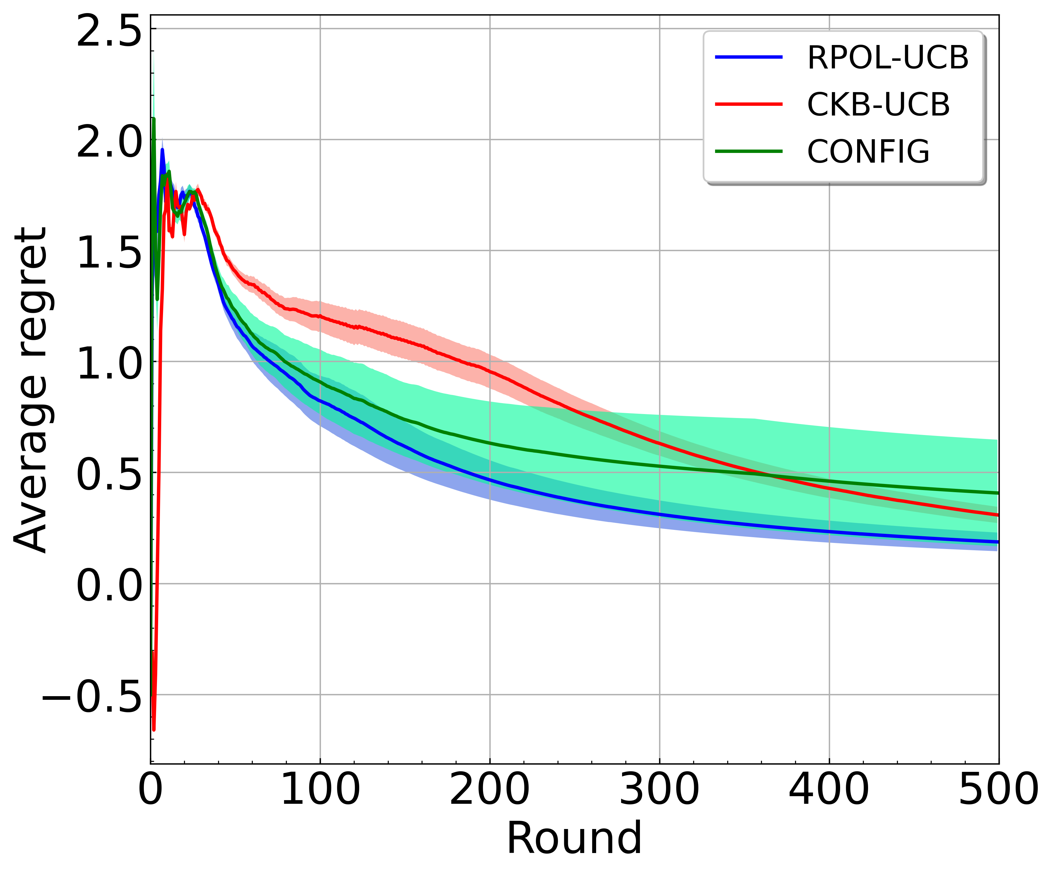
(a) Average Regret

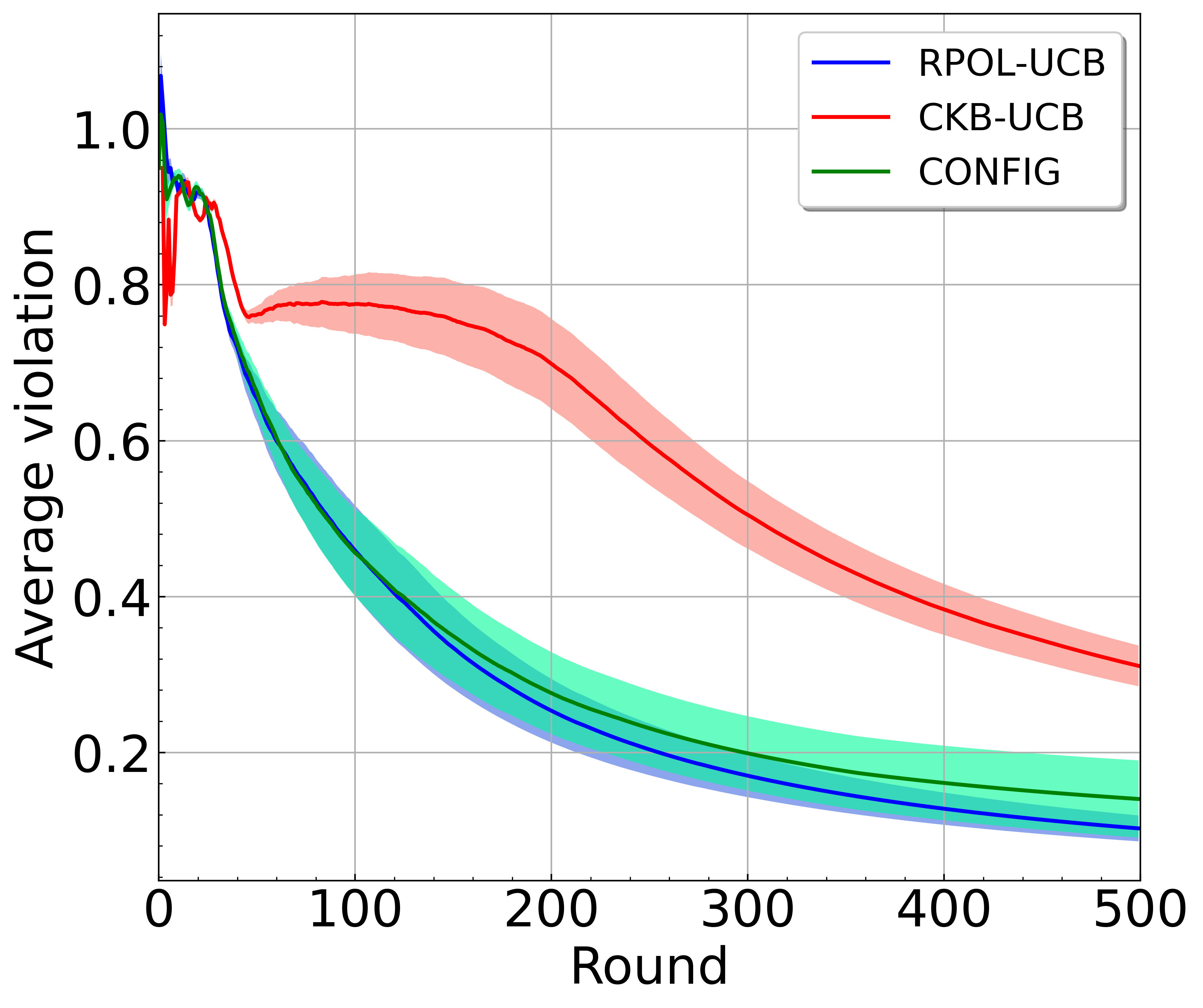
(b) Average Violation

Figure 1: Regret and Cumulative Violation in SCBwC

SCBwC with delayed feedback We consider the stochastic delayed feedback based on the first experiment, where the delay of $d_{t}^{f}$ and $d_{t}^{g}$ at round $t$ are sampled from a Poisson distribution with mean $15,$ respectively. We test RPOL-CensoredUCB and consider RPOL-UCB, CKB-UCB, and CONFIG as the baseline algorithms. From 2(a) and 2(b), RPOL-CensoredUCB also outperforms all existing baselines. These results indicate RPOL framework can establish a strong performance guarantee even with stochastic delayed feedback.

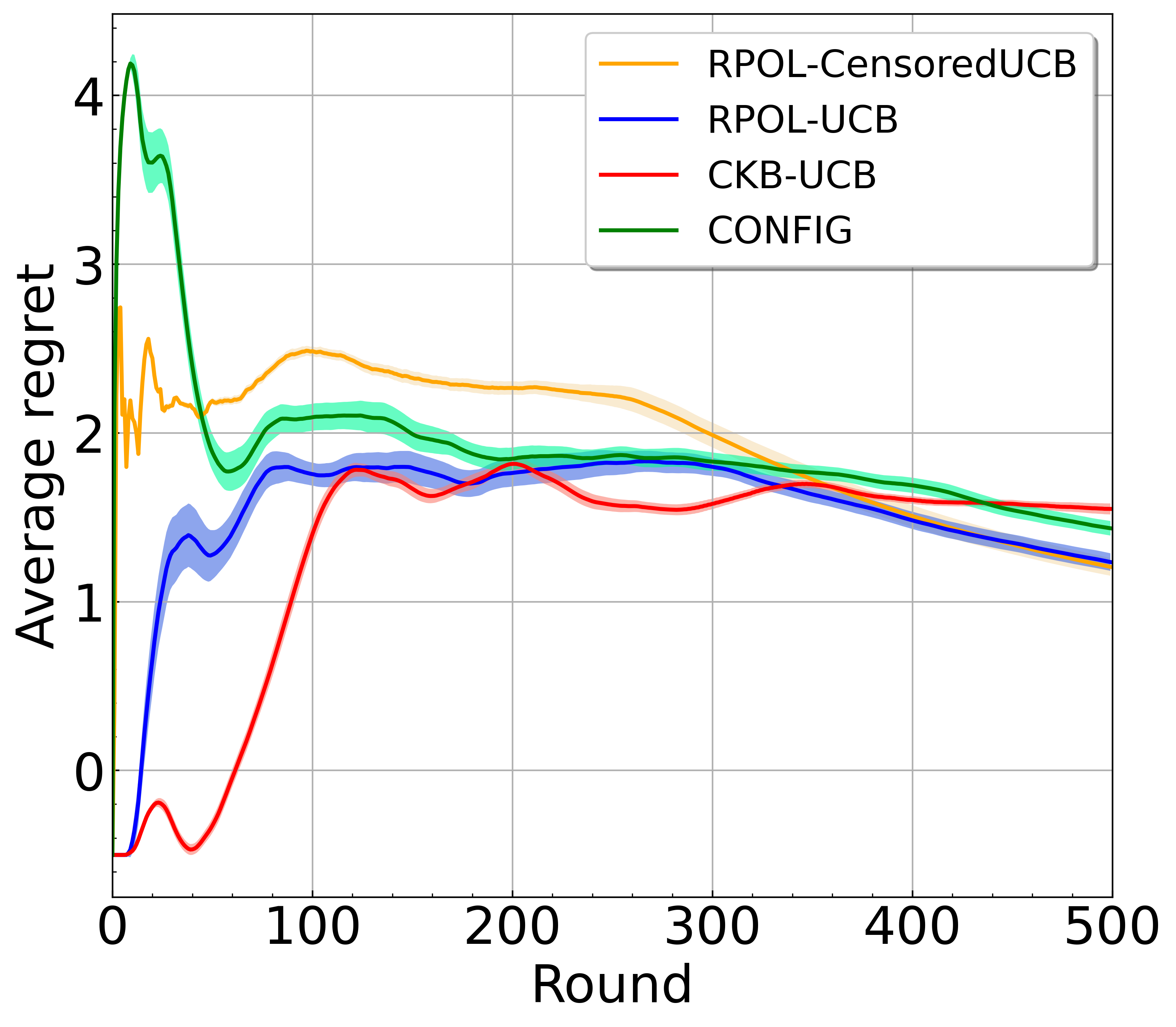
(a) Average Regret

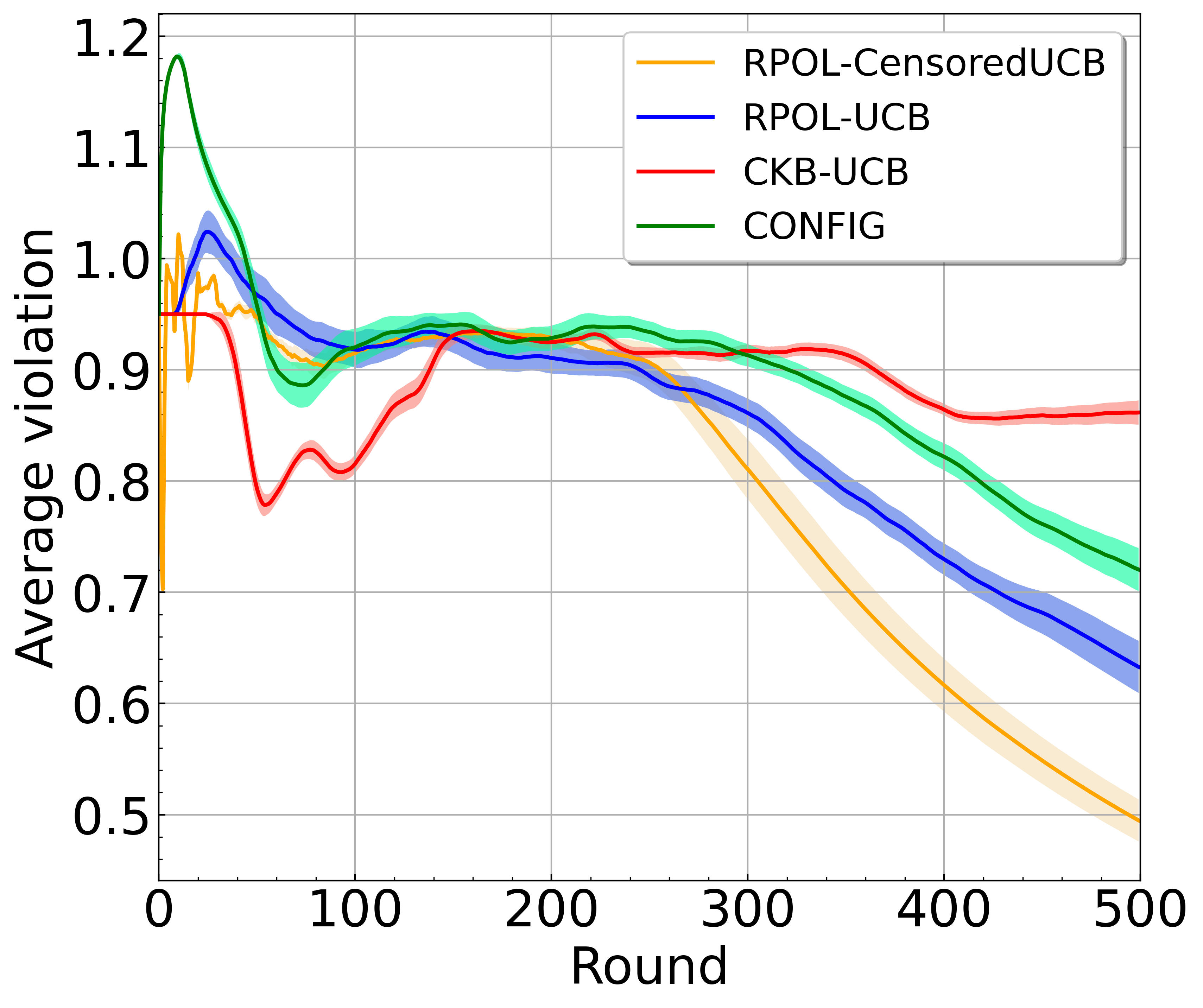
(b) Average Violation

Figure 2: Regret and Cumulative Violation in SCBwC with Delayed Feedback

SCBwC under non-stationary environment We consider the non-stationarity based on the first experiment, where the reward function and constraint function vary at $100$ and $300$ round. Specifically, we set $f_{1:100}=-\sin x(1)-x(2)$; $g_{1:100}=\sin x(1)\sin x(2)+0.95$; $f_{101:300}=-\sin(x(1)-5)-x(2)$; $g_{101:300}=\sin x(1)\sin(x(2)+5)+0.5$; $f_{301:500}=-\sin(x(1)+4)-x(2)$; $g_{301:500}=\sin(x(1)+5)\sin(x(2))+0.95$. We test RPOL-SWUCB and consider CKB-UCB, CONFIG, and CKB-RestartUCB in [8]. From 3(a) and 3(b), we again observe that RPOL-SWUCB has the best performance. It demonstrates that our RPOL framework is flexible and efficient in the non-stationary environment.

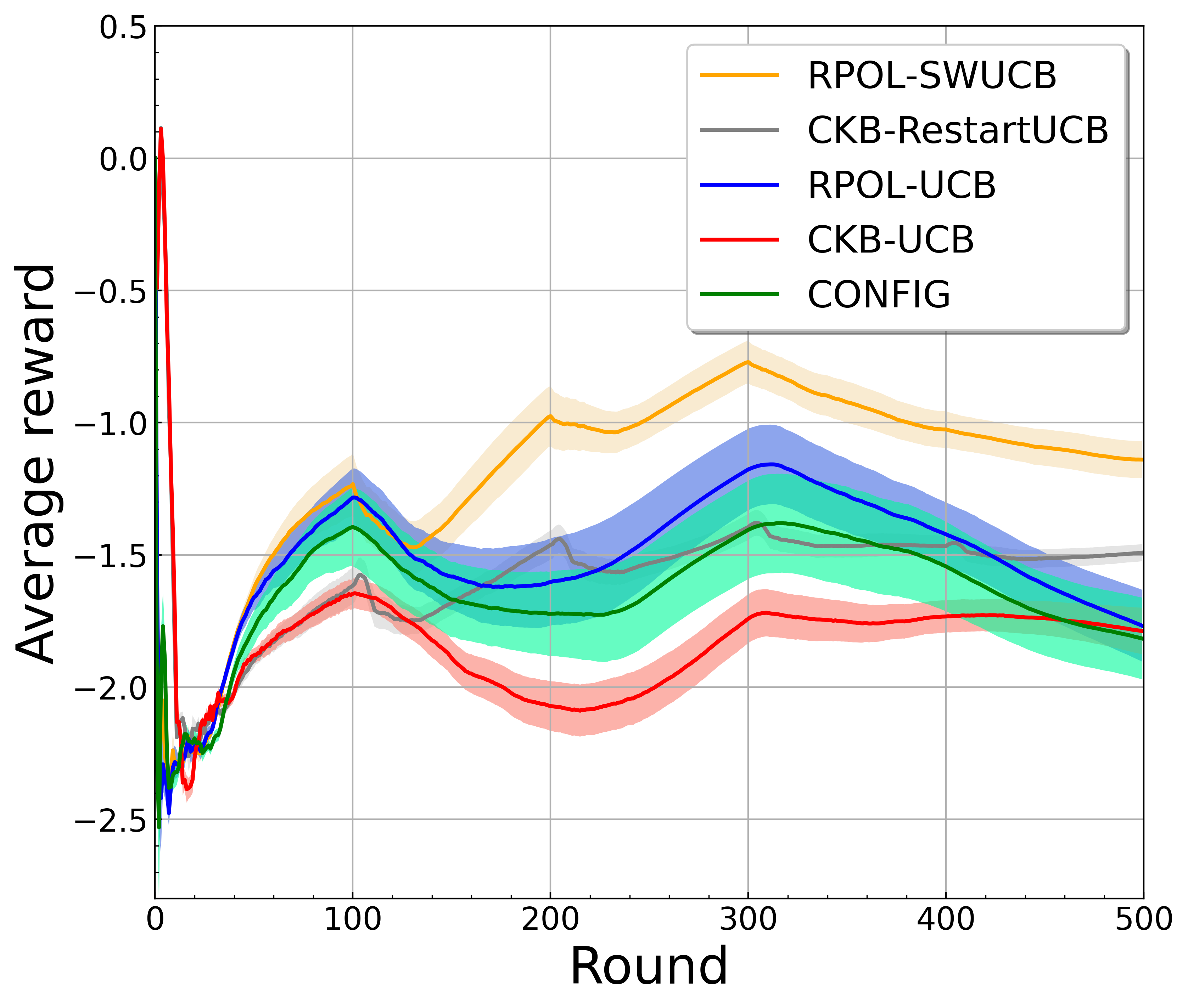
(a) Average Reward

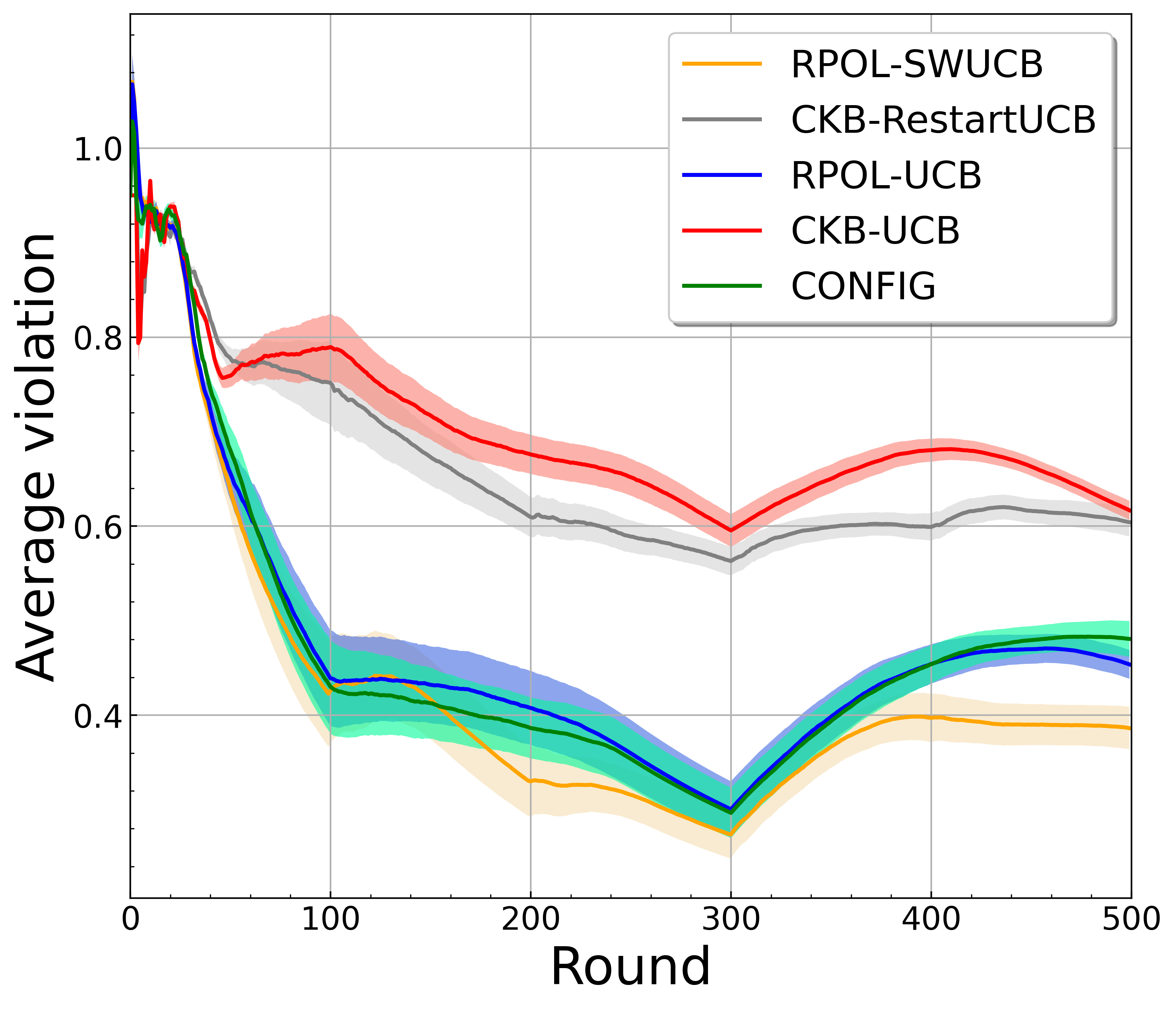
(b) Average Violation

Figure 3: Regret and Cumulative Violation in SCBwC under Non-stationary Environment

8 Conclusion

In this paper, we study stochastic continuum-armed bandit with constraints with the cumulative constraint violation. We propose the rectified pessimistic-optimistic learning framework and show it is flexible to be applied into stochastic continuum-armed bandit with constraints and its variants by utilizing the dedicated exploration techniques. We develop unified analysis techniques to show our framework is efficient in achieving sublinear regret and cumulative violation. Our theoretical and experimental results justify the superior of the proposed framework.

Appendix A Proof of Theorem 1

To prove Theorem 1, we first introduce a key “self-bounding property” to establish an upper bound on “regret + cumulative violation”, motivated by [11].
Self-bounding property: From the decision choice of $x_{t}$ in (11), we have for any $x\in\mathcal{X}$ such that

$$\hat{f}_{t}(x)-Q_{t}\check{g}^{+}_{t}(x)\leq\hat{f}_{t}(x_{t})-Q_{t}\check{g}^{+}_{t}(x_{t}),~{}\forall t\in[T].$$

Let $x=x^{*}$ and add $\rho(f(x^{*})-f(x_{t}))$ to both sides of the inequality above

$$\rho(f(x^{*})-f(x_{t}))+\hat{f}_{t}(x^{*})-Q_{t}\check{g}^{+}_{t}(x^{*})$$

$$\leq \rho(f(x^{*})-f(x_{t}))+\hat{f}_{t}(x_{t})-Q_{t}\check{g}^{+}_{t}(x_{t}).$$

From Condition 1, we have

$$\check{g}_{t}(x^{*})\leq g_{t}(x^{*})\leq 0,~{}\forall t\in[T].$$

hold with a high probability at least $1-p.$ Since $Q_{t}\geq 1$ according to its definition, we rearrange the inequality above and have for any $t\in[T]$

$$\rho(f(x^{*})-f(x_{t}))+Q_{t}\check{g}^{+}_{t}(x_{t})$$

$$\leq \rho f(x^{*})-\hat{f}_{t}(x^{*})+\hat{f}_{t}(x_{t})-\rho f(x_{t}).$$ (15)

Based on the “self-bounding property” in (15), we establish the regret and violation in Theorem 1.

Regret bound: Since $Q_{t}\geq 1,$ we have $Q_{t}\check{g}^{+}_{t}(x_{t})\geq 0.$ The inequality (15) implies

$$\rho(f(x^{*})-f(x_{t}))$$

$$\leq \rho f(x^{*})-\hat{f}_{t}(x^{*})+\hat{f}_{t}(x_{t})-\rho f(x_{t}).$$

From Condition 1, we have $f(x^{*})-\hat{f}_{t}(x^{*})\leq 0$ and $\hat{f}_{t}(x_{t})-f(x_{t})\leq e_{t}^{f}(x_{t})$ for all $t\in[T]$ with the probability at least $1-p.$ We have

$$\mathcal{R}(T):= \frac{1}{\rho}\sum_{t=1}^{T}\rho(f(x^{*})-f(x_{t}))$$

$$\leq \frac{1}{\rho}\sum_{t=1}^{T}(\hat{f}_{t}(x_{t})-\rho f(x_{t}))+\frac{1}{\rho}\sum_{t=1}^{T}(\rho f(x^{*})-\hat{f}_{t}(x^{*}))$$

$$\leq \frac{1}{\rho}\sum_{t=1}^{T}e_{t}^{f}(x_{t})$$

holds with the probability at least $1-p.$
Violation bound: We first establish the upper bound of $\sum_{t=1}^{T}\check{g}^{+}_{t}(x_{t})$ and then connect it with $\sum_{t=1}^{T}g^{+}_{t}(x_{t}).$

Rearrange inequality (15) and we have:

$$Q_{t}\check{g}^{+}_{t}(x_{t})\leq \rho f(x^{*})-\hat{f}_{t}(x^{*})+\hat{f}_{t}(x_{t})-\rho f(x_{t})$$

$$+\rho(f(x_{t})-f(x^{*})),$$

which, conjunction with Condition 1, implies

$$\check{g}^{+}_{t}(x_{t})\leq\frac{e_{t}^{f}(x_{t})+\rho(f(x_{t})-f(x^{*}))}{Q_{t}}.$$

Since $Q_{t}\geq\eta_{t}=\sqrt{t}$ according to the definition, we have

$$\sum_{t=1}^{T}\check{g}^{+}_{t}(x_{t})\leq \sum_{t=1}^{T}\frac{e_{t}^{f}(x_{t})}{\sqrt{t}}+\rho\sum_{t=1}^{T}\frac{f(x_{t})-f(x^{*})}{\sqrt{t}}$$

$$\leq \sum_{t=1}^{T}e_{t}^{f}(x_{t})+4\rho B_{f}\sqrt{T},$$ (16)

where the last inequality holds because (i) $t\geq 1;$ (ii) $f$ is bounded by $B_{f}$ in Assumption 1; and (iii) $\sum_{t=1}^{T}\frac{1}{\sqrt{t}}\leq\int_{1}^{T}\frac{1}{\sqrt{t}}dt\leq 2\sqrt{T}$.

Next, we establish violation based on the relationship between $\check{g}^{+}_{t}(x_{t})$ and ${g}^{+}(x_{t})$ in Condition 1 as follows

$$\mathcal{V}(T):= \frac{1}{\rho}\sum_{t=1}^{T}\rho g^{+}(x_{t})$$

$$= \frac{1}{\rho}\sum_{t=1}^{T}(\rho g(x_{t})-\check{g}_{t}(x_{t})+\check{g}_{t}(x_{t}))^{+}$$

$$\leq \frac{1}{\rho}\sum_{t=1}^{T}(\rho g(x_{t})-\check{g}_{t}(x_{t}))^{+}+\sum_{t=1}^{T}\check{g}_{t}^{+}(x_{t})$$

$$\leq \frac{1}{\rho}\sum_{t=1}^{T}e_{t}^{g}(x_{t})+\sum_{t=1}^{T}\check{g}_{t}^{+}(x_{t})$$

$$\leq \sum_{t=1}^{T}e_{t}^{f}(x_{t})+4\rho B_{f}\sqrt{T}+\frac{1}{\rho}\sum_{t=1}^{T}e_{t}^{g}(x_{t})$$

where the first inequality holds because $(a+b)^{+}\leq(a)^{+}+(b)^{+};$ the second inequality holds because of Condition 1; the last inequality holds by (16).

Appendix B Proof of Theorem 2

In this section, we prove regret bound and violation bound for RPOL with GP-UCB (RPOL-UCB) for SCBwC by Theorem 1. To invoke Theorem 1, we need to verify Condition 1 by proving Lemmas 1 and 2.

B.1 Proof of Lemma 1

Lemma 1 establishes the confidence bounds for estimators $\hat{f}_{t}(\cdot)$ and $\check{g}_{t}(\cdot)$. We first prove for the reward function $f$ and the analysis for the constraint function $g$ follows the same steps.

According to $\hat{f}_{t}(x)=\mu^{f}_{t}(x)+\beta^{f}_{t}\sigma^{f}_{t}(x)$, we have

$$\hat{f}_{t}(x)-f(x)=\mu_{t}^{f}(x)-f(x)+\beta_{t}^{f}\sigma_{t}^{f}(x).$$

Recall that the reward function $f$ lies in RKHS. For convenience, we define $\varphi(x)=k^{f}(x,\cdot)$ instead of $\varphi^{f}(x)$, it implies $f(x)=\langle f,k^{f}(x,\cdot)\rangle_{k^{f}}=\langle f,\varphi(x)\rangle_{k^{f}}:=f^{T}\varphi(x).$ Further define the RKHS norm $\|g\|_{k^{f}}$ as $\sqrt{g^{T}g}$, $\Phi_{t}=[\varphi(x_{1})^{T},\ldots,\varphi(x_{t-1})^{T}]^{T}$, then kenerl matrix $K^{f}_{t}=\Phi_{t}\Phi_{t}^{T}$, $k^{f}_{t}(x)=\Phi_{t}\varphi(x)$ for all $x\in\mathcal{X}$ and $f_{1:t}=\Phi_{t}f$. Since $\mu^{f}_{t}(x)=k^{f}_{t}(x)^{T}(K_{t}^{f}+\lambda I)^{-1}r_{1:t}$, and $r_{1:t}=f_{1:t}+\varepsilon_{1:t}$, we have

$$\mu_{t}^{f}(x)-f(x)=k^{f}_{t}(x)^{T}(K_{t}^{f}+\lambda I)^{-1}f_{1:t}-f(x)+k^{f}_{t}(x)^{T}(K_{t}^{f}+\lambda I)^{-1}\varepsilon_{1:t},$$ (17)

From Theorem 2 in [7], we derive the difference term in (17) as follows

$$|k^{f}_{t}(x)^{T}(K_{t}^{f}+\lambda I)^{-1}f_{1:t}-f(x)| =|\varphi(x)^{T}\Phi_{t}^{T}(\Phi_{t}\Phi_{t}^{T}+\lambda I)^{-1}\Phi_{t}f-\varphi(x)^{T}f|$$

$$=|\varphi(x)^{T}(\Phi_{t}^{T}\Phi_{t}+\lambda I)^{-1}\Phi_{t}^{T}\Phi_{t}f-\varphi(x)^{T}f|$$

$$=|\lambda\varphi^{T}(\Phi_{t}^{T}\Phi_{t}+\lambda I)^{-1}f|$$

$$\leq\|\lambda(\Phi_{t}^{T}\Phi_{t}+\lambda I)^{-1}\varphi(x)\|_{k^{f}}\|f\|_{k^{f}}$$

$$=\|f\|_{k^{f}}\sqrt{\lambda\varphi(x)^{T}(\Phi_{t}^{T}\Phi_{t}+\lambda I)^{-1}\lambda I(\Phi_{t}^{T}\Phi_{t}+\lambda I)^{-1}\varphi(x)}$$

$$\leq B_{f}\sqrt{\lambda\varphi(x)^{T}(\Phi_{t}^{T}\Phi_{t}+\lambda I)^{-1}(\Phi_{t}^{T}\Phi_{t}+\lambda I)(\Phi_{t}^{T}\Phi_{t}+\lambda I)^{-1}\varphi(x)}$$

$$=B_{f}\sigma^{f}_{t}(x),$$

where the second equality comes from the fact that $\Phi_{t}^{T}(\Phi_{t}\Phi_{t}^{T}+\lambda I)^{-1}=(\Phi_{t}^{T}\Phi_{t}+\lambda I)^{-1}\Phi_{t}^{T}$ and the third equality comes from $\varphi(x)=\Phi_{t}^{T}(\Phi_{t}\Phi_{t}^{T}+\lambda I)^{-1}k_{t}^{f}(x)+\lambda(\Phi_{t}^{T}\Phi_{t}+\lambda I)^{-1}\varphi(x),$ and this implies $\lambda\varphi(x)^{T}(\Phi_{t}^{T}\Phi_{t}+\lambda I)^{-1}\varphi(x)=k^{f}(x,x)-k^{f}_{t}(x)^{T}(K_{t}^{f}+\lambda I)^{-1}k_{t}^{f}(x)=(\sigma^{f}_{t}(x))^{2}$ and prove the last equality.

For the second term in (17), we have

$$|k^{f}_{t}(x)^{T}(K_{t}^{f}+\lambda I)^{-1}\varepsilon_{1:t}| =|\varphi(x)^{T}\Phi_{t}^{T}(\Phi_{t}\Phi_{t}^{T}+\lambda I)^{-1}\varepsilon_{1:t}|$$

$$=|\varphi(x)^{T}(\Phi_{t}\Phi_{t}^{T}+\lambda I)^{-1}\Phi_{t}^{T}\varepsilon_{1:t}|$$

$$\leq\|(\Phi_{t}\Phi_{t}^{T}+\lambda I)^{-1/2}\varphi(x)\|_{k^{f}}\|(\Phi_{t}\Phi_{t}^{T}+\lambda I)^{-1/2}\Phi_{t}^{T}\varepsilon_{1:t}\|_{k^{f}}$$

$$=\sqrt{\varphi(x)^{T}(\Phi_{t}^{T}\Phi_{t}+\lambda I)^{-1}\varphi(x)}\sqrt{(\Phi_{t}^{T}\varepsilon_{1:t})^{T}(\Phi_{t}^{T}\Phi_{t}+\lambda I)^{-1}\Phi_{t}^{T}\varepsilon_{1:t}}$$

$$=\lambda^{-1/2}\sigma^{f}_{t}(x)\sqrt{\varepsilon_{1:t}^{T}K_{t}^{f}(K_{t}^{f}+\lambda I)^{-1}\varepsilon_{1:t}}$$

$$\leq\lambda^{-1/2}\sigma^{f}_{t}(x)\sqrt{\varepsilon_{1:t}^{T}(K_{t}^{f}+\eta I)(K_{t}^{f}+\lambda I)^{-1}\varepsilon_{1:t}}$$

$$\leq\sigma^{f}_{t}(x)\sqrt{\varepsilon_{1:t}^{T}((K^{f}_{t}+(2/T)I)^{-1}+I)^{-1}\varepsilon_{1:t}}$$

$$\leq\sigma^{f}_{t}(x)\|\varepsilon_{1:t}\|_{((K^{f}_{t}+(2/T)I)^{-1}+I)^{-1}},$$

where the first inequality comes from $\Phi_{t}^{T}(\Phi_{t}\Phi_{t}^{T}+\lambda I)^{-1}=(\Phi_{t}^{T}\Phi_{t}+\lambda I)^{-1}\Phi_{t}^{T}$ and $\lambda\varphi(x)^{T}(\Phi_{t}^{T}\Phi_{t}+\lambda I)^{-1}\varphi(x)=k^{f}(x,x)-k^{f}_{t}(x)^{T}(K_{t}^{f}+\lambda I)^{-1}k_{t}^{f}(x)$. According to Theorem 1 in [7], we have for any $x\in\mathcal{X}$ and for all $t\in[T]$

$$|k^{f}_{t}(x)^{T}(K_{t}^{f}+\lambda I)^{-1}\varepsilon_{1:t}|\leq R_{f}\sqrt{2(\gamma^{f}_{t}+1+\ln(2/p))}\sigma^{f}_{t}(x)$$

holds with the probability at least $1-p/2.$ Recall the definition of $\beta^{f}_{t},$ we have for any $x\in\mathcal{X}$ and for all $t\in[T]$

$$-\beta^{f}_{t}\sigma^{f}_{t}(x)+\beta^{f}_{t}\sigma^{f}_{t}(x)\leq\hat{f}_{t}(x)-f(x)\leq\beta^{f}_{t}\sigma^{f}_{t}(x)+\beta^{f}_{t}\sigma^{f}_{t}(x).$$

holds with the probability at least $1-p/2.$ Follow the same steps for the constraint function of $g,$ we complete the proof.

B.2 Proof of Lemma 2

We prove the first inequality on reward function $f$ in Lemma 2 and the second inequality on $g$ holds by following the same steps. By Cauchy-Schwartz inequality, we have

$$\sum_{t=1}^{T}\sigma^{f}_{t}(x_{t})\leq\sqrt{T\sum_{t=1}^{T}(\sigma_{t}^{f}(x_{t}))^{2}},$$

From Lemma 3 in [7], we have

$$\gamma^{f}_{t}\geq\frac{1}{2}\sum_{s=1}^{t}\ln{(1+\lambda^{-1}(\sigma^{f}_{s}(x_{s})))^{2}}$$

Combine these facts and $a\leq 2\ln(1+a),~{}\forall a>0,$ we have

$$\sum_{t=1}^{T}\sigma^{f}_{t}(x_{t})\leq \sqrt{2T\lambda\sum_{t=1}^{T}\ln{(1+\lambda^{-1}(\sigma^{f}_{t}(x_{t}))^{2}}}$$

$$\leq \sqrt{4T\lambda\gamma^{f}_{T}}.$$

Recall that $\beta_{t}^{f}$ is increasing with time step $t$ and $\lambda=1+2/T.$ We have

$$\sum_{t=1}^{T}\beta_{t}^{f}\sigma_{t}^{f}(x_{t})\leq\beta_{T}^{f}\sqrt{4(T+2)\gamma_{T}^{f}}.$$

Similarly, we also have

$$\sum_{t=1}^{T}\beta_{t}^{g}\sigma_{t}^{g}(x_{t})\leq\beta_{T}^{g}\sqrt{4(T+2)\gamma_{T}^{g}}.$$

Therefore, we complete the proof.

B.3 Proving Theorem 2

From Lemma 1, we have justified Condition 1 for Theorem 1. Specifically, we have $\rho=1$, $e_{t}^{f}(x)=2\beta^{f}_{t}\sigma^{f}_{t}(x),$ and $e_{t}^{g}(x)=2\beta^{g}_{t}\sigma^{g}_{t}(x)$ in Condition 1. From Lemma 2, we establish the bounds of $\sum_{t=1}^{T}e^{f}_{t}(x_{t})$ and $\sum_{t=1}^{T}e^{g}_{t}(x_{t})$. Now we invoke Theorem 1 to have

$$\mathcal{R}(T) =2\beta_{T}^{f}\sqrt{4(T+2)\gamma_{T}^{f}},$$

$$\mathcal{V}(T) =2\beta_{T}^{f}\sqrt{4(T+2)\gamma_{T}^{f}}+2\beta_{T}^{g}\sqrt{4(T+2)\gamma_{T}^{g}}+4B_{f}\sqrt{T},$$

which completes the proof.

Appendix C Proof of Theorem 3

In this section, we study SCBwC with delayed feedback, and we establish regret and violation bounds for RPOL-CensoredUCB. The detailed algorithm of RPOL-CensoredUCB is shown as follows.   RPOL-CensoredUCB for SCBwC with Delayed Feedback  

Initialization: $\mu^{f}_{1}(x)=\mu^{g}_{1}(x)=0$, $\sigma^{f}_{1}(x)=\sigma^{g}_{1}(x)=1$, $\forall x$, $Q_{1}=1$, $\eta_{t}=\sqrt{t},$ $v_{t}^{f}$ and $v_{t}^{g}$.

For $t=1,\cdots,T,$

• Pessimistic-optimistic learning: estimate the reward $\hat{f}_{t}(x)$ and the cost $\check{g}_{t}(x)$ with GP-UCB/LCB.

  $$\hat{f}_{t}(x)=\mu^{f}_{t}(x)+v^{f}_{t}\sigma^{f}_{t}(x),~{}\check{g}_{t}(x)=\mu^{g}_{t}(x)-v^{g}_{t}\sigma^{g}_{t}(x)$$

• Rectified penalty-based decision: choose $x_{t}$ such that

  $$x_{t}=\operatorname*{arg\,max}_{x\in\mathcal{X}}~{}\hat{f}_{t}(x)-Q_{t}\check{g}^{+}_{t}(x)$$

• Feedback: noisy delayed rewards $r_{s}(x_{s})$ and constraints $c_{l}(x_{l})$ revealed at time $t,$ i.e., $t=s+d^{f}_{s}$ and $t=l+d^{g}_{l}$.

• Rectified cumulative penalty update:

  $$Q_{t+1}=\max(Q_{t}+\sum_{l\in\mathcal{L}}{c}_{l}^{+}(x_{l}),\eta_{t}),$$

  where $\mathcal{L}=\{l\in[T]~{}|~{}t=l+d^{g}_{l}\}.$

• Posterior model update: update $(\mu^{f}_{t+1},\sigma^{f}_{t+1})$ and $(\mu^{g}_{t+1},\sigma^{g}_{t+1})$ with censored feedback $\tilde{r}_{1:t+1}$ and $\tilde{c}_{1:t+1}$:

  $$\mu^{f}_{t+1}(x)=k^{f}_{t+1}(x)^{T}(V_{t+1}^{f}(\lambda))^{-1}\tilde{r}_{1:t+1},~{}\mu^{g}_{t}(x)=k^{g}_{t+1}(x)^{T}(V_{t+1}^{g}(\lambda))^{-1}\tilde{c}_{1:t+1},$$

  $$k^{f}_{t+1}(x,x^{\prime})=k^{f}(x,x^{\prime})-k^{f}_{t+1}(x)^{T}(V_{t+1}^{f}(\lambda))^{-1}k^{f}_{t+1}(x^{\prime}),$$

  $$k^{g}_{t+1}(x,x^{\prime})=k^{g}(x,x^{\prime})-k^{g}_{t+1}(x)^{T}(V_{t+1}^{g}(\lambda))^{-1}k^{g}_{t+1}(x^{\prime}),$$

  $$\sigma_{t+1}^{f}(x)=\sqrt{k_{t+1}^{f}(x,x)},~{}\sigma_{t+1}^{g}(x)=\sqrt{k_{t+1}^{g}(x,x)},$$

  where $K^{f}_{t+1}:=[k^{f}(x,x^{\prime})]_{x,x^{\prime}\in\{x_{1},\cdots,x_{t}\}},$ and $V_{t+1}^{f}(\lambda):=K^{f}_{t+1}+\lambda I,$ $\tilde{r}_{1:t+1}=[\tilde{r}_{1,t},\cdots,\tilde{r}_{t,t}]$, $k^{f}_{t+1}(x):=[k^{f}(x_{1},x),\cdots,k^{f}(x_{t},x)]^{T},$ $K^{g}_{t+1}:=[k^{g}(x,x^{\prime})]_{x,x^{\prime}\in\{x,\cdots,x_{t}\}},$ and $V_{t+1}^{g}(\lambda):=K^{g}_{t+1}+\lambda I,$ $\tilde{c}_{1:t+1}=[\tilde{c}_{1,t},\cdots,\tilde{c}_{t,t}]$, $k^{g}_{t+1}(x):=[k^{g}(x_{1},x),\cdots,k^{g}(x_{t},x)]^{T},$ $\tilde{r}_{s,t+1}:=r_{s}\mathbb{I}\{d^{f}_{s}\leq\min(m,t+1-s)\}$ and $\tilde{c}_{s,{t+1}}:=c_{s}\mathbb{I}\{d^{g}_{s}\leq\min(m,t+1-s)\}$.

 

C.1 Proof of Lemma 3

Similar to Lemma 1, we justify the results for reward function $f$ and that for the constraint function $g$ follows. We first perform our analysis based on the event $\mathcal{E}:=\{r_{t}\leq B_{r},c_{t}\leq B_{c},\forall t\in[T]\}$. Conditional on $\mathcal{E},$ we have

$$\Phi_{t}^{T}\tilde{r}_{1:t} =\sum_{s=1}^{t-1}\varphi(x_{s})r_{s}\mathbb{I}\{d^{f}_{s}\leq\min(m,t-s)\}$$

$$=\sum_{s=1}^{t-1}\varphi(x_{s})r_{s}\mathbb{I}\{d^{f}_{s}\leq m\}+\sum_{s=t-m}^{t-1}\varphi(x_{s})r_{s}(\mathbb{I}\{d_{s}^{f}\leq t-s\}-\mathbb{I}\{d_{s}^{f}\leq m\})$$

Recall $V_{t}^{f}(\lambda)=(K_{t}^{f}+\lambda I)$, then we have

$$\hat{f}(x)-\rho_{m}f(x)= \mu_{t}^{f}(x)-\rho_{m}f(x)+v_{t}^{f}\sigma^{f}_{t}(x)$$

$$= k^{f}_{t}(x)^{T}(K_{t}^{f}+\lambda I)^{-1}\tilde{r}_{1:t}-\rho_{m}\varphi^{T}(x)f+v_{t}^{f}\sigma^{f}_{t}(x)$$

$$= \varphi(x)^{T}\Phi_{t}V_{t}^{f}(\lambda)^{-1}\tilde{r}_{1:t}-\rho_{m}\varphi^{T}(x)f+v_{t}^{f}\sigma^{f}_{t}(x)$$

$$= \varphi(x)^{T}V_{t}^{f}(\lambda)^{-1}\Phi_{t}^{T}\tilde{r}_{1:t}-\rho_{m}\varphi^{T}(x)f+v_{t}^{f}\sigma^{f}_{t}(x)$$

$$= \varphi(x)^{T}V_{t}^{f}(\lambda)^{-1}(\sum_{s=1}^{t-1}\varphi(x_{s})r_{s}\mathbb{I}\{d^{f}_{s}\leq m\})-\rho_{m}\varphi^{T}(x)f$$

$$+\varphi(x)^{T}V_{t}^{f}(\lambda)^{-1}\sum_{s=t-m}^{t-1}\varphi(x_{s})r_{s}(\mathbb{I}\{d_{s}^{f}\leq t-s\}-\mathbb{I}\{d_{s}^{f}\leq m\})$$

$$+v_{t}^{f}\sigma^{f}_{t}(x).$$

From Eq.(4) in [25], we show that the following inequality hold with probability at least $1-p/4$,

$$|\varphi(x)^{T}V_{t}^{f}(\lambda)^{-1}\sum_{s=t-m}^{t-1}\varphi(x_{s})r_{s}(\mathbb{I}\{d_{s}^{f}\leq t-s\}-\mathbb{I}\{d_{s}^{f}\leq m\})|\leq B_{r}\sigma_{t}(x)\sum_{s=t-m}^{t-1}\sigma_{t}(x_{s}).$$

From Eq.(6) and Eq.(9) in [25], with the probability at least $1-p/4$, we have for all $t$ such that

$$|V_{t}^{f}(\lambda)^{-1}(\sum_{s=1}^{t-1}\varphi(x_{s})r_{s}\mathbb{I}\{d^{f}_{s}\leq m\})-\rho_{m}\varphi^{T}(x)f|\leq(B_{f}+(R_{f}+B_{r})\sqrt{2(\gamma_{t}^{f}+1+\ln(4/p))})\sigma^{f}_{t}(x).$$

Recall $v^{f}_{t}=B_{r}\sum_{s=t-m}^{t-1}\sigma^{f}_{t}(x_{s})+\beta^{f}_{t}$ and $\beta^{f}_{t}=B_{f}+(R_{f}+B_{r})\sqrt{2(\gamma^{f}_{t}+1+\ln{(4/p)})}$, we prove that

$$0\leq\hat{f}_{t}(x)-\rho^{f}_{m}f(x)\leq 2v^{f}_{t}\sigma^{f}_{t}(x),\forall t\in[T],$$

holds with the probability at least $1-p/2$. Similarly,

$$0\leq\rho^{g}_{m}g_{t}(x)-\check{g}_{t}(x)\leq 2v^{g}_{t}\sigma^{g}_{t}(x),\forall t\in[T],$$

holds with the probability at least $1-p/2$.

Next, we consider the complement of the event $\mathcal{E},$ i.e., $\mathcal{\bar{E}}.$ According to sub-Gaussian properties in Assumption 2, we have for all $t\in[T]$

$$\mathbb{P}(d^{f}_{t}\geq d_{f})\leq e^{-\frac{d_{f}^{2}}{2R_{f}^{2}}},~{}\mathbb{P}(d^{g}_{t}\geq d_{g})\leq e^{-\frac{d_{g}^{2}}{2R_{g}^{2}}}.$$

Therefore, we choose $B_{r}=B_{f}+R_{f}\sqrt{2\log T}$ and $B_{c}=B_{g}+R_{g}\sqrt{2\log T}$ such that $\mathbb{P}(\mathcal{\bar{E}})\leq 2/T$.

By combining the analysis on the two events $\mathcal{E}$ and $\mathcal{\bar{E}},$ we conclude that Lemma 3 holds with probability at least $1-p-2/T$ according to the union bound.

C.2 Proof of Lemma 4

Similar to Lemma 2, we prove the first inequality on reward function $f$ in Lemma 4 and the second inequality on $g$ holds by following the same steps. Recall that $v^{f}_{t}=B_{r}\sum_{s=t-m}^{t-1}\sigma^{f}_{t-1}(x_{s})+\beta^{f}_{t}$, we have

$$\sum_{t=1}^{T}v_{t}^{f}\sigma_{t}^{f}(x_{t})=\sum_{t=1}^{T}\beta_{t}^{f}\sigma_{t}^{f}(x_{t})+\sum_{t=1}^{T}\sigma_{t}^{f}(x_{t})(B_{r}\sum_{s=t-m}^{t-1}\sigma_{t}(x_{s})).$$ (18)

For the first term in (18), we establish the following inequality by Lemma 2

$$\sum_{t=1}^{T}\beta_{t}^{f}\sigma_{t}^{f}(x)\leq\beta_{T}^{f}\sqrt{4T\lambda\gamma^{f}_{T}}.$$

For the second term in (18), we have the following analysis

$$\sum_{t=1}^{T}\sigma_{t}^{f}(x)(B_{r}\sum_{s=t-m}^{t-1}\sigma_{t}(x_{s})) =B_{r}\sum_{t=1}^{T}\sum_{s=t-m}^{t-1}\sigma_{t}^{f}(x_{t})\sigma_{t}^{f}(x_{s})$$

$$\leq\frac{B_{r}}{2}\sum_{t=1}^{T}\sum_{s=t-m}^{t-1}(\sigma_{t}^{f}(x_{t})^{2}+\sigma_{t}^{f}(x_{s})^{2})$$

$$\leq\frac{B_{r}}{2}\sum_{t=1}^{T}\sum_{s=t-m}^{t-1}(\sigma_{t}^{f}(x_{t})^{2}+\sigma_{s}^{f}(x_{s})^{2})$$

$$\leq mB_{r}\sum_{t=1}^{T}\sigma_{t}^{f}(x_{t})^{2}$$

$$\leq mB_{r}4\lambda\gamma_{T}^{f},$$

where the last inequality holds since $\sum_{t=1}^{T}\sigma_{t}^{f}(x_{t})^{2}\leq\lambda\sum_{t=1}^{T}2\ln{(1+\lambda^{-1}(\sigma^{f}_{t}(x_{t}))^{2})}\leq 4\lambda\gamma_{T}^{f}$.
Then we have

$$\sum_{t=1}^{T}v_{t}^{f}\sigma_{t}^{f}(x)\leq\beta_{T}^{f}\sqrt{4T\lambda\gamma^{f}_{T}}+mB_{r}4\lambda\gamma_{T}^{f}.$$

Similarly, we have the inequality for $g$ function

$$\sum_{t=1}^{T}v_{t}^{g}\sigma_{t}^{g}(x)\leq\beta_{T}^{g}\sqrt{4T\lambda\gamma^{g}_{T}}+mB_{c}4\lambda\gamma_{T}^{g}.$$

Therefore, we complete the proof.

C.3 Proving Theorem 3

From Lemma 3, we have justified Condition 1 for Theorem 1. Specifically, we have $\rho=\rho_{m}$, $e_{t}^{f}(x)=2v^{f}_{t}\sigma^{f}_{t}(x)$ and $e_{t}^{g}(x_{t})=2v^{g}_{t}\sigma^{g}_{t}(x)$ in Condition 1. From Lemma 4, we establish the bounds of $\sum_{t=1}^{T}e^{f}_{t}(x_{t})$ and $\sum_{t=1}^{T}e^{g}_{t}(x_{t})$. Now we invoke Theorem 1 and prove

$$\mathcal{R}(T)=2\beta_{T}^{f}\sqrt{4T\lambda\gamma^{f}_{T}}+mB_{r}8\lambda\gamma_{T}^{f},$$

$$\mathcal{V}(T)=2\beta_{T}^{f}\sqrt{4T\lambda\gamma^{f}_{T}}+mB_{r}8\lambda\gamma_{T}^{f}+2\beta_{T}^{g}\sqrt{4T\lambda\gamma^{g}_{T}}+mB_{c}8\lambda\gamma_{T}^{g}+4B_{f}\sqrt{T}.$$

Appendix D Proof of Theorem 4

In this section, we study SCBwC under non-stationary environment. We establish regret and violation bounds for RPOL-SWUCB. The detailed algorithm of RPOL-SWUCB is shown as follows.   RPOL-SWUCB for SCBwC under Non-stationary Environment  

Initialization: $\mu^{f}_{1}(x)=\mu^{g}_{1}(x)=0$, $\sigma^{f}_{1}(x)=\sigma^{g}_{1}(x)=1$, $\forall x$, $Q_{1}=1$, window size $W$, $\eta_{t}=\sqrt{t},$ $\beta_{t}^{f}$, $\beta_{t}^{g}$, $\Gamma_{t}^{f}$ and $\Gamma_{t}^{g}$.

For $t=1,\cdots,T,$

• Pessimistic-optimistic learning: estimate the reward $\hat{f}_{t}(x)$ and the cost $\check{g}_{t}(x)$ with sliding window GP-UCB/LCB.

  $$\hat{f}_{t}(x)=\mu^{f}_{t}(x)+\beta^{f}_{t}\sigma^{f}_{t}(x)+\Gamma_{t}^{f},~{}\check{g}_{t}(x)=\mu^{g}_{t}(x)-\beta^{g}_{t}\sigma^{g}_{t}(x)-\Gamma_{t}^{g}.$$

• Rectified penalty-based decision: choose $x_{t}$ such that

  $$x_{t}=\operatorname*{arg\,max}_{x\in\mathcal{X}}~{}\hat{f}_{t}(x)-Q_{t}\check{g}^{+}_{t}(x)$$

• Feedback: noisy reward $r_{t}(x_{t})$ and cost $c_{t}(x_{t}).$

• Rectified penalty update:

  $$Q_{t+1}=\max\left(Q_{t}+c_{t}^{+}(x_{t}),\eta_{t}\right).$$

• Posterior model update: update $(\mu^{f}_{t+1},\sigma^{f}_{t+1})$ and $(\mu^{g}_{t+1},\sigma^{g}_{t+1})$ with $r_{t_{0}:t+1}$ and $c_{t_{0}:t+1}$, where $t_{0}=1\vee(t-W)$:

  $$\mu^{f}_{t+1}(x)=k^{f}_{t+1}(x)^{T}(V_{t+1}^{f}(\lambda))^{-1}r_{t_{0}:t+1},~{}\mu^{g}_{t+1}(x)=k^{g}_{t+1}(x)^{T}(V_{t+1}^{g}(\lambda))^{-1}c_{t_{0}:t+1},$$

  $$k^{f}_{t+1}(x,x^{\prime})=k^{f}(x,x^{\prime})-k^{f}_{t+1}(x)^{T}(V_{t+1}^{f}(\lambda))^{-1}k^{f}_{t+1}(x^{\prime}),$$

  $$k^{g}_{t+1}(x,x^{\prime})=k^{g}(x,x^{\prime})-k^{g}_{t+1}(x)^{T}(V_{t+1}^{g}(\lambda))^{-1}k^{g}_{t+1}(x^{\prime}),$$

  $$\sigma_{t+1}^{f}(x)=\sqrt{k_{t+1}^{f}(x,x)},~{}\sigma_{t+1}^{g}(x)=\sqrt{k_{t+1}^{g}(x,x)},$$

  where $k^{f}_{t+1}(x):=[k^{f}(x_{t_{0}},x),\cdots,k^{f}(x_{t},x)]^{T},$ $K^{f}_{t+1}:=[k^{f}(x,x^{\prime})]_{x,x^{\prime}\in\{x_{t_{0}},\cdots,x_{t}\}},$ and $V_{t+1}^{f}(\lambda):=K^{f}_{t+1}+\lambda I;$ $k^{g}_{t+1}(x):=[k^{g}(x_{t_{0}},x),\cdots,k^{g}(x_{t},x)]^{T},$ $K^{g}_{t+1}:=[k^{g}(x,x^{\prime})]_{x,x^{\prime}\in\{x_{t_{0}},\cdots,x_{t}\}},$ and $V_{t+1}^{g}(\lambda):=K^{g}_{t+1}+\lambda I.$

 

D.1 Proof of Lemma 5

With a bit abuse of notion, we define $\Phi_{t}=[\varphi(x_{t_{0}})^{T},\ldots,\varphi(x_{t-1})^{T}]^{T}.$ Recall $f_{t}(x)=f_{t}^{T}\varphi(x)$, $\mu_{t}^{f}(x)=k^{f}_{t}(x)^{T}(V_{t}^{f}(\lambda))^{-1}r_{t_{0}:t}=\varphi(x)^{T}V_{t}^{f}(\lambda)^{-1}\Phi_{t}^{T}r_{t_{0}:t}$. Next, we study $\hat{f}_{t}(x)-f(x)$ as follows

$$\hat{f}_{t}(x)-f(x)= \mu_{t}^{f}(x)-f_{t}(x)+\beta^{f}_{t}\sigma_{t}^{f}(x)+\Gamma_{t}^{f}$$

$$= \varphi(x)^{T}V_{t}^{f}(\lambda)^{-1}\Phi_{t}^{T}r_{t_{0}:t}-\varphi(x)^{T}f_{t}+\beta^{f}_{t}\sigma_{t}^{f}(x)+\Gamma_{t}^{f}$$

$$= \varphi(x)^{T}V_{t}^{f}(\lambda)^{-1}(\sum_{s=t_{0}}^{t-1}\varphi(x_{s})\varphi(x_{s})^{T}(f_{s}-f_{t}))+\varphi(x)^{T}V_{t}^{f}(\lambda)^{-1}\varepsilon_{t_{0}:t}-\lambda\varphi^{T}(x)V_{t}^{f}(\lambda)^{-1}f_{t}$$

$$+\beta^{f}_{t}\sigma_{t}^{f}(x)+\Gamma_{t}^{f}.$$

From Eq.(9) in [36], we have

$$|\varphi(x)^{T}V_{t}^{f}(\lambda)^{-1}(\sum_{s=t_{0}}^{t-1}\varphi(x_{s})\varphi(x_{s})^{T}(f_{s}-f_{t}))|\leq\frac{1}{\lambda}\sqrt{W2(1+\lambda)\gamma_{T}^{f}}\sum_{s=t_{0}}^{t-1}\|f_{s}-f_{s+1}\|_{k^{f}}.$$

Then from Eq.(6) and Eq.(7) in [36], we have

$$|\lambda\varphi^{T}(x)V_{t}^{f}(\lambda)^{-1}f_{t}|\leq B_{f}\sigma_{t}^{f}(x),$$

$$|\varphi(x)^{T}V_{t}^{f}(\lambda)^{-1}\varepsilon_{t_{0}:t}|\leq\frac{1}{\sqrt{\lambda}}R_{f}\sqrt{2\gamma^{f}_{t-t_{0}}+2\ln(2T/p)}.$$

Recall the value of $\beta_{t}^{f}$ and $\Gamma_{t}^{f}$, we prove that with the probability at least $1-p/2$,

$$0\leq\hat{f}_{t}(x)-f_{t}(x)\leq 2\Gamma^{f}_{t}+2\beta^{f}_{t}\sigma^{f}_{t}(x),\forall t\in[T].$$

Similarly,

$$0\leq g_{t}(x)-\check{g}_{t}(x)\leq 2\Gamma^{g}_{t}+2\beta^{g}_{t}\sigma^{g}_{t}(x),\forall t\in[T]$$

holds with the probability at least $1-p/2$. Therefore, we have completed the proof according to the union bound.

D.2 Proof of Lemma 6

We first justify the upper bounds of $\sum_{t=1}^{T}\Gamma^{f}_{t}$ and $\sum_{t=1}^{T}\beta^{f}_{t}\sigma^{f}_{t}(x_{t})$ for the reward function $f$ and the analysis for the constraint function $g$ follows the exact steps. Let $C_{f}:=\frac{1}{\lambda}\sqrt{W2(1+\lambda)\gamma^{f}_{T}}.$ We have

$$\sum_{t=1}^{T}\frac{1}{\lambda}\sqrt{2W(1+\lambda)\gamma^{f}_{T}}\sum_{s=t_{0}}^{t-1}\|f_{s}-f_{s+1}\|_{k^{f}}=C_{f}\sum_{t=1}^{T}\sum_{s=t_{0}}^{t-1}\|f_{s}-f_{s+1}\|_{k^{f}},$$

where $t_{0}=1\vee(t-W)$. Combine with the fact that $\sum_{t=1}^{T}\sum_{s=t_{0}}^{t-1}\|f_{s}-f_{s+1}\|_{k^{f}}\leq WP_{T}$ and recall the definition of $P_{T}=\max(\sum_{t=1}^{T}\|f_{t+1}-f_{t}\|_{k^{f}},\sum_{t=1}^{T}\|g_{t+1}-g_{t}\|_{k^{g}}),$ we establish

$$C_{f}\sum_{t=1}^{T}\sum_{s=t_{0}}^{t-1}\|f_{s}-f_{s+1}\|_{k^{f}}\leq C_{f}WP_{T}.$$

Next, we provide the bound of $\sum_{t=1}^{T}\beta^{f}_{t}\sigma^{f}_{t}(x_{t}).$ Note we have

$$\sum_{t=1}^{T}\beta^{f}_{t}\sigma^{f}_{t}(x_{t})=\sum_{t=1}^{T}\beta^{f}_{t}2\sqrt{\lambda}\|\varphi(x_{t})\|_{(K_{t_{0}:t}^{f}+\lambda I)^{-1}},$$

where $\varphi(\cdot)$ is the same as we define in Appendix B.1 and $K_{t_{0}:t}^{f}=\sum_{s=t_{0}}^{t-1}\varphi(x_{s})\varphi(x_{s})^{T}$.

$$\sum_{t=1}^{T}\beta^{f}_{t}2\sqrt{\lambda}\|\varphi(x_{t})\|_{(K_{t_{0},t}^{f}+\lambda I)^{-1}}\leq\beta_{T}^{f}2\sqrt{\lambda}\sum_{k=0}^{T/W-1}\sum_{t=kW+1}^{(k+1)W}\|\varphi(x_{t})\|_{(K_{t_{0},t}^{f}+\lambda I)^{-1}}$$

We define $K^{f}_{kW+1:t}=\sum_{s=kW+1}^{t-1}\varphi(x_{s})\varphi(x_{s})^{T}$, then for $t\in[kW,(k+1)W]$. We have $(K_{t_{0}:t}^{f}+\lambda I)^{-1}\preceq(K^{f}_{kW+1:t}+\lambda I)^{-1}$ such that

$$\sum_{t=kW+1}^{(k+1)W}\|\varphi(x_{t})\|_{(K_{t_{0}:t}^{f}+\lambda I)^{-1}}\leq\sum_{t=kW+1}^{(k+1)W}\|\varphi(x_{t})\|_{(K^{f}_{kW+1:t}+\lambda I)^{-1}}.$$

Now we study every individual block (e.g., $k$-block ranges from $kW+1$ to $(k+1)W$) separately and use Lemma 2 to conclude

$$\sum_{t=kW+1}^{(k+1)W}\|\varphi(x_{t})\|_{(K^{f}_{kW+1:t}+\lambda I)^{-1}}=\frac{1}{\sqrt{\lambda}}\sum_{t=kW+1}^{(k+1)W}\sigma^{f}_{t-kW}(x_{t})\leq\sqrt{4T\gamma^{f}_{T}},$$

Combine all these facts, then we prove that

$$\sum_{t=1}^{T}\beta^{f}_{t}\sigma^{f}_{t}(x_{t})\leq(T/W)\beta_{T}^{f}\sqrt{4W\gamma^{f}_{T}}=\beta_{T}^{f}T\sqrt{\frac{4\gamma_{T}^{f}}{W}}.$$

D.3 Proving Theorem 4

Lemmas 5 and 6 establish the following error bounds hold with probability at least $1-p$

$$\sum_{t=1}^{T}\Gamma^{f}_{t}+\beta^{f}_{t}\sigma^{f}_{t}(x_{t})\leq C_{f}WP_{T}+\beta_{T}^{f}T\sqrt{\frac{4\gamma_{T}^{f}}{W}},$$

$$\sum_{t=1}^{T}\Gamma^{g}_{t}+\beta^{f}_{t}\sigma^{g}_{t}(x_{t})\leq C_{g}WP_{T}+\beta_{T}^{g}T\sqrt{\frac{4\gamma_{T}^{g}}{W}}.$$

Recall $C_{f}=\frac{1}{\lambda}\sqrt{W2(1+\lambda)\gamma^{f}_{T}}$ and $C_{g}=\frac{1}{\lambda}\sqrt{W2(1+\lambda)\gamma^{g}_{T}}$. By invoking Theorem 1, we have

$$\mathcal{R}(T)=2C_{f}WP_{T}+2\beta_{T}^{f}T\sqrt{\frac{4\gamma_{T}^{f}}{W}}+4B_{f}\sqrt{T},$$

$$\mathcal{V}(T)=2C_{g}WP_{T}+2\beta_{T}^{g}T\sqrt{\frac{4\gamma_{T}^{g}}{W}}+2C_{f}WP_{T}+2\beta_{T}^{f}T\sqrt{\frac{4\gamma_{T}^{f}}{W}}+4B_{f}\sqrt{T}.$$

Let the window size $W=\gamma_{T}^{1/4}(T/P_{T})^{1/2}$ and we have

$$\mathcal{R}(T)\leq 4(1+\beta^{f}_{T})\gamma_{T}^{3/4}P_{T}^{1/4}T^{3/4}+4B_{f}\sqrt{T},$$

$$\mathcal{V}(T)\leq 4(2+\beta^{f}_{T}+\beta^{g}_{T})\gamma_{T}^{3/4}P_{T}^{1/4}T^{3/4}+4B_{f}\sqrt{T}.$$

holds with the probability at least $1-p.$ The proof is completed.

References

• [1] Sanae Amani, Mahnoosh Alizadeh, and Christos Thrampoulidis. Regret bound for safe gaussian process bandit optimization. In Learning for Dynamics and Control, pages 158–159. PMLR, 2020.
• [2] Setareh Ariafar, Jaume Coll-Font, DanaΒ H Brooks, and JenniferΒ G Dy. Admmbo: Bayesian optimization with unknown constraints using admm. The Journal of Machine Learning Research, 20(123):1–26, 2019.
• [3] Felix Berkenkamp, Andreas Krause, and AngelaΒ P Schoellig. Bayesian optimization with safety constraints: safe and automatic parameter tuning in robotics. Machine Learning, pages 1–35, 2021.
• [4] Xuanyu Cao, Junshan Zhang, and H.Β Vincent Poor. Online stochastic optimization with time-varying distributions. IEEE Transactions on Automatic Control, 66(4):1840–1847, 2021.
• [5] WangΒ Chi Cheung, David Simchi-Levi, and Ruihao Zhu. Learning to optimize under non-stationarity. In Kamalika Chaudhuri and Masashi Sugiyama, editors, Proceedings of the Twenty-Second International Conference on Artificial Intelligence and Statistics, volumeΒ 89 of Proceedings of Machine Learning Research. PMLR, 16–18 Apr 2019.
• [6] WangΒ Chi Cheung, David Simchi-Levi, and Ruihao Zhu. Hedging the drift: Learning to optimize under nonstationarity. Management Science, 68(3):1696–1713, 2022.
• [7] SayakΒ Ray Chowdhury and Aditya Gopalan. On kernelized multi-armed bandits. In International Conference on Machine Learning, pages 844–853. PMLR, 2017.
• [8] Yuntian Deng, Xingyu Zhou, Arnob Ghosh, Abhishek Gupta, and NessΒ B Shroff. Interference constrained beam alignment for time-varying channels via kernelized bandits. arXiv preprint arXiv:2207.00908, 2022.
• [9] Audrey Durand, Charis Achilleos, Demetris Iacovides, Katerina Strati, GeorgiosΒ D. Mitsis, and Joelle Pineau. Contextual bandits for adapting treatment in a mouse model of de novo carcinogenesis. In Proceedings of the 3rd Machine Learning for Healthcare Conference, volumeΒ 85 of Proceedings of Machine Learning Research, pages 67–82. PMLR, 17–18 Aug 2018.
• [10] Xinzhe Fu and Eytan Modiano. Learning-num: Network utility maximization with unknown utility functions and queueing delay. MobiHoc ’21, New York, NY, USA, 2021. Association for Computing Machinery.
• [11] Hengquan Guo, Xin Liu, Honghao Wei, and Lei Ying. Online convex optimization with hard constraints: Towards the best of two worlds and beyond. In Thirty-Sixth Conference on Neural Information Processing Systems, 2022.
• [12] EricΒ C. Hall and RebeccaΒ M. Willett. Dynamical models and tracking regret in online convex programming. In Proceedings of the 30th International Conference on Machine Learning, ICML, 2013.
• [13] Andreas Krause and Cheng Ong. Contextual gaussian process bandit optimization. In J.Β Shawe-Taylor, R.Β Zemel, P.Β Bartlett, F.Β Pereira, and K.Q. Weinberger, editors, Advances in Neural Information Processing Systems, volumeΒ 24. Curran Associates, Inc., 2011.
• [14] Nikolaos Liakopoulos, Apostolos Destounis, Georgios Paschos, Thrasyvoulos Spyropoulos, and Panayotis Mertikopoulos. Cautious regret minimization: Online optimization with long-term budget constraints. In Proceedings of the 36th International Conference on Machine Learning. ICML, 2019.
• [15] Shang Liu, Jiashuo Jiang, and Xiaocheng Li. Non-stationary bandits with knapsacks. In Advances in Neural Information Processing Systems, 2022.
• [16] Congwen Lu and JoelΒ A. Paulson. No-regret bayesian optimization with unknown equality and inequality constraints using exact penalty functions. IFAC-PapersOnLine, 2022. 13th IFAC Symposium on Dynamics and Control of Process Systems.
• [17] Mehrdad Mahdavi, Rong Jin, and Tianbao Yang. Trading regret for efficiency: online convex optimization with long term constraints. The Journal of Machine Learning Research, 13(1):2503–2528, 2012.
• [18] MichaelΒ J Neely and Hao Yu. Online convex optimization with time-varying constraints. arXiv preprint arXiv:1702.04783, 2017.
• [19] Omid Sadeghi, Prasanna Raut, and Maryam Fazel. A single recipe for online submodular maximization with adversarial or stochastic constraints. In Advances in Neural Information Processing Systems, 2020.
• [20] Zai Shi and Atilla Eryilmaz. A bayesian approach for stochastic continuum-armed bandit with long-term constraints. In International Conference on Artificial Intelligence and Statistics, pages 8370–8391. PMLR, 2022.
• [21] Niranjan Srinivas, Andreas Krause, ShamΒ M Kakade, and Matthias Seeger. Gaussian process optimization in the bandit setting: No regret and experimental design. arXiv preprint arXiv:0912.3995, 2009.
• [22] Yanan Sui, Alkis Gotovos, Joel Burdick, and Andreas Krause. Safe exploration for optimization with gaussian processes. In International conference on machine learning, pages 997–1005. PMLR, 2015.
• [23] Yanan Sui, Vincent Zhuang, Joel Burdick, and Yisong Yue. Stagewise safe bayesian optimization with gaussian processes. In International conference on machine learning, pages 4781–4789. PMLR, 2018.
• [24] Wen Sun, Debadeepta Dey, and Ashish Kapoor. Safety-aware algorithms for adversarial contextual bandit. In International Conference on Machine Learning, pages 3280–3288. PMLR, 2017.
• [25] Arun Verma, Zhongxiang Dai, and Bryan KianΒ Hsiang Low. Bayesian optimization under stochastic delayed feedback. In International Conference on Machine Learning, pages 22145–22167. PMLR, 2022.
• [26] Claire Vernade, Alexandra Carpentier, Tor Lattimore, Giovanni Zappella, Beyza Ermis, and Michael BrΓΌckner. Linear bandits with stochastic delayed feedback. In Proceedings of the 37th International Conference on Machine Learning, volume 119 of Proceedings of Machine Learning Research, pages 9712–9721. PMLR, 13–18 Jul 2020.
• [27] Chen-Yu Wei and Haipeng Luo. Non-stationary reinforcement learning without prior knowledge: an optimal black-box approach. In Proceedings of Thirty Fourth Conference on Learning Theory, Proceedings of Machine Learning Research. PMLR, 15–19 Aug 2021.
• [28] Colin White, Willie Neiswanger, and Yash Savani. Bananas: Bayesian optimization with neural architectures for neural architecture search. Proceedings of the AAAI Conference on Artificial Intelligence, 35:10293–10301, May 2021.
• [29] Wenjie Xu, Yuning Jiang, and ColinΒ N Jones. Constrained efficient global optimization of expensive black-box functions. arXiv preprint arXiv:2211.00162, 2022.
• [30] Xinlei Yi, Xiuxian Li, Tao Yang, Lihua Xie, Tianyou Chai, and Karl Johansson. Regret and cumulative constraint violation analysis for online convex optimization with long term constraints. In International Conference on Machine Learning, pages 11998–12008. PMLR, 2021.
• [31] Xinlei Yi, Xiuxian Li, Tao Yang, Lihua Xie, Tianyou Chai, and KarlΒ H Johansson. Regret and cumulative constraint violation analysis for distributed online constrained convex optimization. arXiv preprint arXiv:2105.00321, 2021.
• [32] Jianjun Yuan and Andrew Lamperski. Online convex optimization for cumulative constraints. Advances in Neural Information Processing Systems, 31, 2018.
• [33] Lijun Zhang, Shiyin Lu, and Zhi-Hua Zhou. Adaptive online learning in dynamic environments. In Thirty-Second Conference on Neural Information Processing Systems, 2018.
• [34] Peng Zhao, Lijun Zhang, Yuan Jiang, and Zhi-Hua Zhou. A simple approach for non-stationary linear bandits. In Proceedings of the Twenty Third International Conference on Artificial Intelligence and Statistics, volume 108 of Proceedings of Machine Learning Research, pages 746–755. PMLR, 2020.
• [35] Xingyu Zhou and BoΒ Ji. On kernelized multi-armed bandits with constraints. In Thirty-Sixth Conference on Neural Information Processing Systems, 2022.
• [36] Xingyu Zhou and Ness Shroff. No-regret algorithms for time-varying bayesian optimization. In 2021 55th Annual Conference on Information Sciences and Systems (CISS), 2021.
• [37] Martin Zinkevich. Online convex programming and generalized infinitesimal gradient ascent. In Proceedings of the 20th International Conference on Machine Learning, ICML, 2003.