Spatio-Temporal Meta-Graph Learning for Traffic Forecasting

Abstract

Traffic forecasting as a canonical task of multivariate time series forecasting has been a significant research topic in AI community. To address the spatio-temporal heterogeneity and non-stationarity implied in the traffic stream, in this study, we propose Spatio-Temporal Meta-Graph Learning as a novel Graph Structure Learning mechanism on spatio-temporal data. Specifically, we implement this idea into Meta-Graph Convolutional Recurrent Network (MegaCRN) by plugging the Meta-Graph Learner powered by a Meta-Node Bank into GCRN encoder-decoder. We conduct a comprehensive evaluation on two benchmark datasets (i.e., METR-LA and PEMS-BAY) and a new large-scale traffic speed dataset called EXPY-TKY that covers 1843 expressway road links in Tokyo. Our model outperformed the state-of-the-arts on all three datasets. Besides, through a series of qualitative evaluations, we demonstrate that our model can explicitly disentangle the road links and time slots with different patterns and be robustly adaptive to any anomalous traffic situations. Codes and datasets are available at https://github.com/deepkashiwa20/MegaCRN.

Introduction

Spatio-temporal data, streamed by sensor networks, are widely studied in both academia and industry given various real-world applications. Traffic forecasting (Yu, Yin, and Zhu 2018; Li et al. 2018; Zheng et al. 2020; Bai et al. 2020; Lee et al. 2022), as one canonical task, has been receiving increasing attention with rapid developing Graph Convolutional Networks (GCNs) (Defferrard, Bresson, and Vandergheynst 2016; Kipf and Welling 2017; Veličković et al. 2017). This spatio-temporal modeling task can be formulated similarly to multivariate time series (MTS) forecasting (Wu et al. 2020; Cao et al. 2020; Shang, Chen, and Bi 2021), but with extra prior knowledge from the geographic space (e.g. sensor locations, road networks) to imply the dependency among sensor signals. Compared with ordinary MTS, traffic data (e.g. traffic speed and flow) potentially contain spatio-temporal heterogeneity, as traffic condition differs over roads (e.g. local road, highway, interchange) and time (e.g. off-peak and rush hours). Moreover, non-stationarity makes the task even more challenging when X factors, including accident and congestion, present.

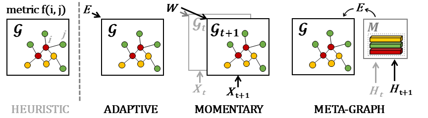
Figure 1: Progression of Graph Structure Learning for Spatio-Temporal Modeling

For more effective traffic forecasting, the existing works have made tremendous progress by modeling latent spatial correlation among sensors and temporal autocorrelation within time series. Since these two relationships can be naturally represented by graph and sequence respectively, the mainstream models handle them by leveraging GCN-based modules (Diao et al. 2019; Guo et al. 2019; Geng et al. 2019; Zhang et al. 2021) and sequence models, such as Recurrent Neural Networks (RNNs) (Li et al. 2018; Bai et al. 2020; Ye et al. 2021), WaveNet (Wu et al. 2019), Transformer (Zheng et al. 2020; Wang et al. 2020; Xu et al. 2020). Particularly, to perform convolution-like operations on graphs, GCNs require an auxiliary input that characterizes the topology of the underlying spatial dependency. This essential part is defined based on certain metrics in early works, such as inverse-distance Gaussian kernel (Yu, Yin, and Zhu 2018; Li et al. 2018), cosine similarity (Geng et al. 2019).

However, this pre-defined graph not only relies on empirical laws (e.g. Tobler’s first law of geography) which does not necessarily indicate an optimal solution, but ignores the dynamic nature of traffic networks. This twofold limitation has stimulated explorations in two lines of research. The first one aims to find the optimal graph structure that facilitates the forecasting task. GW-Net (Wu et al. 2019) pioneers along this direction by treating the adjacency matrix as free variables (i.e. parameterized node embedding $E$) to train, which generates a so-called adaptive graph (in Figure 1). Models including MTGNN (Wu et al. 2020), AGCRN (Bai et al. 2020), GTS (Shang, Chen, and Bi 2021) fall into this category, integrating MTS and traffic forecasting with Graph Structure Learning (GSL) (Zhu et al. 2021). In the other line of research, attempts have been made to tackle network dynamics using matrix or tensor decomposition (Diao et al. 2019; Ye et al. 2021) and attention mechanisms (Guo et al. 2019; Zheng et al. 2020). Motivated by GSL, recent models like SLCNN (Zhang et al. 2020), StemGNN (Cao et al. 2020) further try to learn a time-variant graph structure from observational data. The spatio-temporal graph (STG) derived in this way is essentially input-conditioned, in which parameters denoted by $W$ project observations into node embeddings (termed as momentary graph in Figure 1).

Thus far, while spatio-temporal regularities have been studied systematically, spatio-temporal heterogeneity and non-stationarity have not been tackled properly. Although the heterogeneity issue can be alleviated to some extent by applying attentions over the space and time (Guo et al. 2019; Zheng et al. 2020), sensor signals of different natures are still left entangled, not to mention that incidents are simply untreated. Therefore, we are motivated to propose a novel spatio-temporal meta-graph learning framework. The term meta-graph is coined to describe the generation of node embeddings (similar in adaptive and momentary) for GSL. Specifically, our STG learning consists of two steps: (1) querying node-level prototypes from a Meta-Node Bank; (2) reconstructing node embeddings with Hyper-Network (Ha, Dai, and Le 2016). This localized memorizing capability empowers our modularized Meta-Graph Learner to essentially distinguish traffic patterns on different roads over time, which is even generalizable to incident situations. Our contributions are highlighted as follows:

• We propose a novel Meta-Graph Learner for spatio-temporal graph (STG) learning, to explicitly disentangles the heterogeneity in space and time.

• We present a generic Meta-Graph Convolutional Recurrent Network (MegaCRN), which simply relies on observational data to be robust and adaptive to any traffic situation, from normal to non-stationary.

• We validate MegaCRN quantitatively and qualitatively over a group of state-of-the-art models on two benchmarks (METR-LA and PEMS-BAY) and our newly published dataset (EXPY-TKY) that has larger scale and more complex incident situations.

Related Work

Traffic Forecasting. Traffic forecasting has been taken as a significant research problem in transportation engineering (Huang et al. 2014; Lv et al. 2014; Ma et al. 2015b). As a canonical case of multivariate time series forecasting (Lai et al. 2018), it also has drawn a lot of attention from machine learning researchers. At the very beginning, statistical models including autoregressive model (AR) (Hamilton and Susmel 1994), vector autoregression (VAR) (Stock and Watson 2001), autoregressive integrated moving average (ARIMA) (Pan, Demiryurek, and Shahabi 2012) were applied. Then deep learning methods come to dominate the time series prediction by automatically extracting the non-linear complex features from the data. First, LSTM (Hochreiter and Schmidhuber 1997) and GRU (Chung et al. 2014) demonstrated superior performance in traffic modeling (Ma et al. 2015a; Lv et al. 2018; Li et al. 2018; Zhao et al. 2019; Wang et al. 2020; Bai et al. 2020; Ye et al. 2021; Shang, Chen, and Bi 2021; Lee et al. 2022) as well as multivariate time series forecasting (Lai et al. 2018; Shih, Sun, and Lee 2019). Second, instead of the RNNs, Temporal Convolution (Yu and Koltun 2016) and WaveNet (Oord et al. 2016) with long receptive field were also utilized as the core component in (Yu, Yin, and Zhu 2018; Wu et al. 2019, 2020; Lu et al. 2020; Deng et al. 2021) for temporal modeling. Third, motivated by (Vaswani et al. 2017), a series of traffic transformers (Zheng et al. 2020; Xu et al. 2020) and time series transformers (Li et al. 2019; Zhou et al. 2021; Xu et al. 2021) were proposed to do the long sequence time series modeling. Due to the space limitation, we refer you to the recent surveys (Jiang et al. 2021; Jiang and Luo 2021; Li et al. 2021) on traffic forecasting with deep learning.

Graph Structure Learning. Besides the sequence modeling, research efforts have been made to capture the correlations among variables (road links in traffic data) via generic graph structures (Kipf et al. 2018). Early methods either rely on the natural topology of the road network (i.e., binary adjacency graph) or pre-defined graphs in certain metrics (e.g., Euclidean distance) (Li et al. 2018; Yu, Yin, and Zhu 2018). Then, GW-Net (Wu et al. 2019) first proposed to use two learnable embedding matrices to automatically build an adaptive graph based on the input traffic data. Following GW-Net (Wu et al. 2019), MTGNN (Wu et al. 2020) and GTS (Shang, Chen, and Bi 2021) further proposed to learn a parameterized k-degree discrete graph, while AGCRN (Bai et al. 2020) introduced node-specific convolution filters according to the node embedding and CCRNN (Ye et al. 2021) learned multiple adaptive graphs for multi-layer graph convolution. StemGNN (Cao et al. 2020) took the self-attention (Vaswani et al. 2017) learned from the input as the latent graph. Our work distinguishes itself from these methods by augmenting the spatio-temporal graph learning with memory network (Meta-Node Bank) to discover latent node-level prototypes and construct memory-tailored node embedding.

Problem Definition

Without loss of generality, we formulate our problem as a multi-step-to-multi-step forecasting task as follows:

$$[X_{t-(\alpha-1)},...,X_{t}]\xrightarrow[\theta]{\quad\mathbb{F}(\cdot)\quad}[X_{t+1},...,X_{t+\beta}]$$ (1)

where $X_{i}$ $\in$ $\mathbb{R}^{N\times C}$, $N$ is the number of spatial units (i.e., nodes, grids, regions, road links, etc.), and $C$ is the number of the information channel. In our case, $C$ is equal to 1 as we only forecast the traffic speed; the spatial unit is road link. To be simple, we omit $C$ in the rest of our paper. Given previous $\alpha$ steps of observations [$X_{t-(\alpha-1)}$,…,$X_{t-1}$,$X_{t}$], we aim to infer the next $\beta$ horizons [$X_{t+1}$,$X_{t+2}$,…,$X_{t+\beta}$] by training a forecasting model $\mathbb{F}$ with parameter $\theta$.

Methodology

In this section, we present a generic framework for spatio-temporal meta-graph learning, namely Meta-Graph Convolutional Recurrent Network (MegaCRN), built upon Graph Convolutional Recurrent Unit (GCRU) Encoder-Decoder and plugin Meta-Graph Learner, as illustrated in Figure 2.

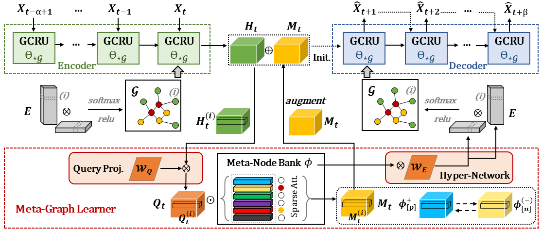
Figure 2: Framework of Meta-Graph Convolutional Recurrent Network (MegaCRN)

Preliminaries

Graph Convolutional Recurrent Unit. Motivated by the success of Graph Convolutional Networks (GCNs) as a class in representation learning on graph-structured data (e.g. social and road networks), a recent line of research (Li et al. 2018; Bai et al. 2020; Shang, Chen, and Bi 2021; Ye et al. 2021) has explored the possibility of injecting graph convolution operation into recurrent cell (e.g. LSTM). The derived Graph Convolutional Recurrent Unit (GCRU) can thereby simultaneously capture spatial dependency, represented by an input graph topology, and temporal dependency in a sequential manner. Without loss of generality, we take the widely adopted definitions of graph convolution operation and Gated Recurrent Unit (GRU) to denote GCRU, as the basic unit for spatio-temporal modeling:

$$H=\sigma(X\star_{\mathcal{G}}\Theta)=\sigma(\mathop{\sum}_{k=0}^{K}\mathcal{\tilde{P}}^{k}X\textit{ }W_{k})$$ (2)

$$\begin{cases}\begin{aligned} u_{t}&=sigmoid([X_{t},\textit{ }H_{t-1}]\star_{\mathcal{G}}\Theta_{u}+b_{u})\\ r_{t}&=sigmoid([X_{t},\textit{ }H_{t-1}]\star_{\mathcal{G}}\Theta_{r}+b_{r})\\ C_{t}&=tanh([X_{t},\textit{ }(r_{t}\odot H_{t-1})]\star_{\mathcal{G}}\Theta_{C}+b_{C})\\ H_{t}&=u_{t}\odot H_{t-1}+(1-u_{t})\odot C_{t}\end{aligned}\end{cases}$$ (3)

In Equation (2), $X\in\mathbb{R}^{N\times C}$ and $H\in\mathbb{R}^{N\times h}$ denote the input and output of graph convolution operation ($\star_{\mathcal{G}}$), in which $\Theta$ or $W_{K}\in\mathbb{R}^{K\times C\times h}$ are the kernel parameters approximated with the Chebyshev polynomials to the order of $K$ (Defferrard, Bresson, and Vandergheynst 2016) and $\sigma$ is an activation function. In Equation (3), subscripts u, r, and C denote update gate, reset gate, and candidate state in a GCRU cell, in which $\Theta_{\{u,r,C\}}\in\mathbb{R}^{K\times(C+h)\times h}$ denote the gate parameters. Besides observation $X_{t}$, GCRU requires an auxiliary input $\mathcal{P}\in\mathbb{R}^{N\times N}$ for the topology of graph $\mathcal{G}$.

Graph Structure Learning. Matrix $\mathcal{P}$ is conventionally defined based on certain metrics (e.g. inverse distance, cosine similarity) and empirical laws (Yu, Yin, and Zhu 2018; Li et al. 2018; Geng et al. 2019). However, choice of metric can be arbitrary and suboptimal, which motivates a line of research (Wu et al. 2020; Zhang et al. 2020; Shang, Chen, and Bi 2021; Bai et al. 2020; Ye et al. 2021) to integrate Graph Structure Learning (GSL) into spatio-temporal modeling for simultaneous optimization. Here we adopt the canonical formulation (Wu et al. 2019; Bai et al. 2020; Wang et al. 2022) for spatio-temporal graph learning, namely adaptive graph (in Figure 1), denoted by:

$$\tilde{\mathcal{P}}=softmax(relu(E\textit{ }E^{\top}))$$ (4)

where $\tilde{\mathcal{P}}$ is derived by random walk normalizing the non-negative part of matrix product of trainable node embedding $E\in\mathbb{R}^{N\times e}$ to its transpose. The other GSL strategy, momentary graph (Zhang et al. 2020) (in Figure 1), can be defined in a similar fashion with input signal $X_{t}$ or hidden state $H_{t}$. Taking the latter as an example:

$$\tilde{\mathcal{P}}_{t}=softmax(relu((H_{t}*W)\textit{ }(H_{t}*W)^{\top}))$$ (5)

where parameter matrix $W\in\mathbb{R}^{h\times e}$ essentially projects $H_{t}$ to another embedding space. Notably, momentary graph has other variants, such as replacing the projection with self-attention operation (Cao et al. 2020), but they still follow Equation (5) as a general form.

Spatio-Temporal Meta-Graph Learner

Here we formally describe a new spatio-temporal graph (STG) learning module. The term meta-graph is coined to represent the generation of node embedding for graph structure learning, which is different from its definition in heterogeneous information networks (HIN) (Zhao et al. 2017; Ding et al. 2021). According to the definition in Equation (4) and (5), adaptive graph relies on parameterized node embedding $E$ alone, while momentary graph is in fact input-conditioned (either projecting $X_{t}$ or $H_{t}$ with parameter $W$). Apparently, this generation process determines the properties of the derived graphs, as the former is time-invariant but the latter is sensitive to input signals. This motivates us to further enhance the node embeddings for STG generation, as the real-world networks are more complex, manifesting spatio-temporal heterogeneity and non-stationarity.

We are inspired by a line of research in memory networks, which aims to memorize typical features in seen samples for further pattern matching. This technique has been largely employed on computer vision tasks, such as few-shot learning (Vinyals et al. 2016; Santoro et al. 2016) and anomaly detection (Gong et al. 2019; Park, Noh, and Ham 2020). In our case, we would like inject the memorizing and distinguishing capabilities into spatio-temporal graph learning. We thereby leverage the idea of memory networks and build a Meta-Node Bank $\Phi\in\mathbb{R}^{\phi\times d}$. Here $\phi$ and $d$ denote the number of memory items and the dimension of each item, respectively. We further define the main functions of this memory bank as follows:

$$Q_{t}^{(i)}=H_{t}^{(i)}*W_{Q}+b_{Q}$$ (6)

$$\begin{cases}\begin{aligned} a_{j}^{(i)}&=\frac{\exp{(Q_{t}^{(i)}*\Phi^{\top}[j])}}{\sum_{j=1}^{\phi}\exp{(Q_{t}^{(i)}*\Phi^{\top}[j])}}\\ M_{t}^{(i)}&=\sum_{j=1}^{\phi}a_{j}^{(i)}*\Phi[j]\end{aligned}\end{cases}$$ (7)

where we use superscript $(i)$ as row index. For instance, $H_{t}^{(i)}\in\mathbb{R}^{h}$ represents $i$-th node vector in $H_{t}\in\mathbb{R}^{N\times h}$. Equation (6) denotes a fully connected (FC parameter $W_{Q}\in\mathbb{R}^{h\times d}$) layer to project hidden state $H_{t}^{(i)}$ to a localized query $Q_{t}^{(i)}\in\mathbb{R}^{d}$. Equation (7) denotes the memory reading operation by matching $Q_{t}^{(i)}$ with each memory $\Phi[j]$ to calculate a scalar $a_{j}$, which physically represents the similarity between vector $Q_{t}^{(i)}$ and memory item $\Phi[j]$. A meta-node vector $M_{t}^{(i)}\in\mathbb{R}^{d}$ can be further recovered as a combination of memory items. Here a common practice is to utilize the reconstructed representation $M_{t}\in\mathbb{R}^{N\times d}$ to augment the encoded hidden representation $H_{t}$, denoted by $H^{\prime}_{t}=[H_{t},M_{t}]\in\mathbb{R}^{N\times(h+d)}$ ($[\cdot]$ denotes a concatenation operation) (Yao et al. 2019; Lee et al. 2022). We further leverage a Hyper-Network (Ha, Dai, and Le 2016) that essentially puts generation of GSL node embeddings conditioned on Meta-Node Bank. This memory-augmented node embedding generation can be formulated as:

$$\begin{cases}\begin{aligned} E^{\prime}&=\textit{NN}_{H}(\Phi)\\ \tilde{\mathcal{P}^{\prime}}&=softmax(relu(E^{{}^{\prime}}\textit{ }E^{{}^{\prime}\top}))\end{aligned}\end{cases}$$ (8)

where $\textit{NN}_{H}$ denotes a Hyper-Network. Without loss of generality, we implement it with one FC layer (parameter $W_{E}\in\mathbb{R}^{d\times e}$). Then, meta-graph $\tilde{\mathcal{P}^{\prime}}$ can be constructed, as an alternative to adaptive and momentary graphs (defined in Equation (4) an (5)) to feed back to GCRU encoder-decoder.

Meta-Graph Convolutional Recurrent Network

With Meta-Graph Learner as described, we present the proposed Meta-Graph Convolutional Recurrent Network (MegaCRN) as a generic framework for spatial-temporal modeling. MegaCRN learns node-level prototypes of traffic patterns in Meta-Node Bank for updating the auxiliary graph adaptively based on the observed situation. To further enhance its distinguishing power for diverse scenarios on different roads over time, we regulate the memory parameters with two constraints (Gong et al. 2019; Park, Noh, and Ham 2020), including a contrastive loss $\mathcal{L}_{1}$ and a consistency loss $\mathcal{L}_{1}$, denoted by:

$$\mathcal{L}_{1} =\mathop{\sum}_{t}^{T}\mathop{\sum}_{i}^{N}\max\{||Q_{t}^{(i)}-\Phi[p]||^{2}-||Q_{t}^{(i)}-\Phi[n]||^{2}+\lambda,0\}$$ (9)

$$\mathcal{L}_{2} =\mathop{\sum}_{t}^{T}\mathop{\sum}_{i}^{N}||Q_{t}^{(i)}-\Phi[p]||^{2}$$

where $T$ denotes the total number of sequences (i.e. samples) in the training set and $p,n$ denote the top two indices of memory items by ranking $a_{j}^{(i)}$ in Equation 7 given localized query $Q_{t}^{(i)}$. By implementing these two constraints, we treat $Q_{t}^{(i)}$ as anchor, its most similar prototype $\Phi[p]$ as positive sample, and the second similar prototype $\Phi[n]$ as negative sample ($\lambda$ denotes the margin between the positive and negative pairs). Here the idea is to keep memory items as compact as possible, at the same time as dissimilar as possible. These two constraints guide memory $\Phi$ to distinguish different spatio-temporal patterns on node-level. In practice, we find adding them into the objective criterion (i.e. MAE) facilitates the convergence of training (with balancing factors $\kappa_{1},\kappa_{2}$):

$$\mathcal{L}_{task}=\mathop{\sum}_{t}^{T}\mathop{\sum}_{\rho}^{\beta}|\hat{X}_{t+\rho}-X_{t+\rho}|+\kappa_{1}\mathcal{L}_{1}+\kappa_{2}\mathcal{L}_{2}$$ (10)

Experiment

Table 1: Summary of Datasets

Dataset	METR-LA	PEMS-BAY	EXPY-TKY
Start Time	2012/3/1	2017/1/1	2021/10/1
End Time	2012/6/30	2017/5/31	2021/12/31
Time Interval	5 minutes	5 minutes	10 minutes
#Timesteps	34,272	52,116	13,248
#Spatial Units	207 sensors	325 sensors	1,843 road links

Table 2: Forecasting Performance

METR-LA	15min / horizon 3			30min / horizon 6			60min / horizon 12
	MAE	RMSE	MAPE	MAE	RMSE	MAPE	MAE	RMSE	MAPE
HA(Li et al. 2018)	4.16	7.80	13.00%	4.16	7.80	13.00%	4.16	7.80	13.00%
STGCN(Yu, Yin, and Zhu 2018)	2.88	5.74	7.62%	3.47	7.24	9.57%	4.59	9.40	12.70%
DCRNN(Li et al. 2018)	2.77	5.38	7.30%	3.15	6.45	8.80%	3.60	7.59	10.50%
GW-Net(Wu et al. 2019)	2.69	5.15	6.90%	3.07	6.22	8.37%	3.53	7.37	10.01%
STTN(Xu et al. 2020)	2.79	5.48	7.19%	3.16	6.50	8.53%	3.60	7.60	10.16%
GMAN(Zheng et al. 2020)$\star$	2.80	5.55	7.41%	3.12	6.49	8.73%	3.44	7.35	10.07%
MTGNN(Wu et al. 2020)	2.69	5.18	6.86%	3.05	6.17	8.19%	3.49	7.23	9.87%
StemGNN(Cao et al. 2020)$\dagger$	2.56	5.06	6.46%	3.01	6.03	8.23%	3.43	7.23	9.85%
AGCRN(Bai et al. 2020)	2.86	5.55	7.55%	3.25	6.57	8.99%	3.68	7.56	10.46%
CCRNN(Ye et al. 2021)	2.85	5.54	7.50%	3.24	6.54	8.90%	3.73	7.65	10.59%
GTS(Shang, Chen, and Bi 2021)$\star$	2.65	5.20	6.80%	3.05	6.22	8.28%	3.47	7.29	9.83%
PM-MemNet(Lee et al. 2022)	2.65	5.29	7.01%	3.03	6.29	8.42%	3.46	7.29	9.97%
MegaCRN (Ours)	2.52	4.94	6.44%	2.93	6.06	7.96%	3.38	7.23	9.72%
PEMS-BAY	15min / horizon 3			30min / horizon 6			60min / horizon 12
	MAE	RMSE	MAPE	MAE	RMSE	MAPE	MAE	RMSE	MAPE
HA(Li et al. 2018)	2.88	5.59	6.80%	2.88	5.59	6.80%	2.88	5.59	6.80%
STGCN(Yu, Yin, and Zhu 2018)	1.36	2.96	2.90%	1.81	4.27	4.17%	2.49	5.69	5.79%
DCRNN(Li et al. 2018)	1.38	2.95	2.90%	1.74	3.97	3.90%	2.07	4.74	4.90%
GW-Net(Wu et al. 2019)	1.30	2.74	2.73%	1.63	3.70	3.67%	1.95	4.52	4.63%
STTN(Xu et al. 2020)	1.36	2.87	2.89%	1.67	3.79	3.78%	1.95	4.50	4.58%
GMAN(Zheng et al. 2020)$\star$	1.35	2.90	2.87%	1.65	3.82	3.74%	1.92	4.49	4.52%
MTGNN(Wu et al. 2020)	1.32	2.79	2.77%	1.65	3.74	3.69%	1.94	4.49	4.53%
StemGNN(Cao et al. 2020)$\dagger$	1.23	2.48	2.63%	N/A from (Cao et al. 2020)			N/A from (Cao et al. 2020)
AGCRN(Bai et al. 2020)	1.36	2.88	2.93%	1.69	3.87	3.86%	1.98	4.59	4.63%
CCRNN(Ye et al. 2021)	1.38	2.90	2.90%	1.74	3.87	3.90%	2.07	4.65	4.87%
GTS(Shang, Chen, and Bi 2021)$\star$	1.34	2.84	2.83%	1.67	3.83	3.79%	1.98	4.56	4.59%
PM-MemNet(Lee et al. 2022)$\star$	1.34	2.82	2.81%	1.65	3.76	3.71%	1.95	4.49	4.54%
MegaCRN (Ours)	1.28	2.72	2.67%	1.60	3.68	3.57%	1.88	4.42	4.41%
EXPY-TKY	10min / horizon 1			30min / horizon 3			60min / horizon 6
	MAE	RMSE	MAPE	MAE	RMSE	MAPE	MAE	RMSE	MAPE
HA(Li et al. 2018)	7.63	11.96	31.26%	7.63	11.96	31.25%	7.63	11.96	31.24%
STGCN(Yu, Yin, and Zhu 2018)	6.09	9.60	24.84%	6.91	10.99	30.24%	8.41	12.70	32.90%
DCRNN(Li et al. 2018)	6.04	9.44	25.54%	6.85	10.87	31.02%	7.45	11.86	34.61%
GW-Net(Wu et al. 2019)	5.91	9.30	25.22%	6.59	10.54	29.78%	6.89	11.07	31.71%
STTN(Xu et al. 2020)	5.90	9.27	25.67%	6.53	10.40	29.82%	6.99	11.23	32.52%
GMAN(Zheng et al. 2020)	6.09	9.49	26.52%	6.64	10.55	30.19%	7.05	11.28	32.91%
MTGNN(Wu et al. 2020)	5.86	9.26	24.80%	6.49	10.44	29.23%	6.81	11.01	31.39%
StemGNN(Cao et al. 2020)$\dagger$	6.08	9.46	25.87%	6.85	10.80	31.25%	7.46	11.88	35.31%
AGCRN(Bai et al. 2020)	5.99	9.38	25.71%	6.64	10.63	29.81%	6.99	11.29	32.13%
CCRNN(Ye et al. 2021)	5.90	9.29	24.53%	6.68	10.77	29.93%	7.11	11.56	32.56%
GTS(Shang, Chen, and Bi 2021)	-	-	-	-	-	-	-	-	-
PM-MemNet(Lee et al. 2022)	5.94	9.25	25.10%	6.52	10.42	29.00%	6.87	11.14	31.22%
MegaCRN (Ours)	5.81	9.20	24.49%	6.44	10.33	28.92%	6.83	11.04	31.02%

Datasets and Settings

Datasets. We first evaluate our model by using two standard benchmark datasets from (Li et al. 2018): METR-LA and PEMS-BAY. They contain the traffic speed data from 207 sensors in Los Angeles and 325 sensors in Bay Area respectively. For the two benchmarks, we follow the tradition (Li et al. 2018; Wu et al. 2019; Shang, Chen, and Bi 2021; Lee et al. 2022) by splitting the datasets in chronological order with 70% for training, 10% for validation, and 20% for testing (namely 7:1:2). Besides, in this study, we publish a new traffic dataset called EXPY-TKY, that contains the traffic speed information and the corresponding traffic incident information in 10-minute interval for 1843 expressway road links in Tokyo over three months (2021/10$\sim$2021/12). We use the first two months (Oct. 2021 and Nov. 2021) as the training and validation dataset, and the last one month (Dec. 2021) as the testing dataset. The specific spatio-temporal information of our datasets are summarized in Table 1.

Settings. For EXPY-TKY, the Encoder and Decoder of our model consist of 1 RNN-layer respectively, where the number of hidden states is 32. We reserve 10 prototypes (i.e., meta-nodes) in the memory, each of which is a 32-dimension learnable vector. For METR-LA and PEMSBAY, each RNN layer in Encoder and Decoder has 64 units and the memory bank has 20 meta-nodes with 64-dimension. The observation step $\alpha$ and prediction horizon $\beta$ are both set to 12 on METR-LA and PEMS-BAY, while $\alpha$/$\beta$ are both set to 6 on EXPY-TKY. Such settings can give us 1-hour lead time forecasting, which follow the tradition in previous literatures (Yu, Yin, and Zhu 2018; Li et al. 2018; Wu et al. 2019; Bai et al. 2020; Shang, Chen, and Bi 2021). Adam was used as the optimizer, where the learning rate was set to 0.01 and the batch size was set to 64. The optimizer would either be early-stopped if the validation error was converged within 20 epochs or be stopped after 200 epochs. L1 Loss is used as the loss function. Root Mean Square Error (RMSE), Mean Absolute Error (MAE), and Mean Absolute Percentage Error (MAPE) are used as metrics. All experiments were performed with four GeForce RTX 3090 GPUs.

Quantitative Evaluation

We compare our model with the following baselines: 1) Historical Average (HA) averaged values of the same time slot from historical days (Li et al. 2018); 2) STGCN (Yu, Yin, and Zhu 2018), 3) DCRNN (Li et al. 2018), and 4) GW-Net (Wu et al. 2019), the most representative deep models for traffic forecasting, respectively embed spectral (Yu, Yin, and Zhu 2018) or diffusion graph convolution (Li et al. 2018; Wu et al. 2019) into temporal convolution (i.e., TCN or WaveNet)(Yu, Yin, and Zhu 2018; Wu et al. 2019) or recurrent unit (e.g., GRU)(Li et al. 2018); 5) STTN (Xu et al. 2020) and 6) GMAN (Zheng et al. 2020) are two Transformer-based SOTAs; 7) MTGNN (Wu et al. 2020) is an extended version of GW-Net that extends the adaptive graph leaning part; 8) StemGNN (Cao et al. 2020) first learns a latent graph via self-attention and performs the spatiotemporal modeling in spectral domain; 9) AGCRN (Bai et al. 2020) adaptively learns node-specific parameters for graph convolution; 10) CCRNN (Ye et al. 2021) learns multiple parameterized matrices for multiple layers of graph convolution; 11) GTS (Shang, Chen, and Bi 2021) learns each link’s (edge’s) probability based on each variable’s (node’s) long historical data; 12) PM-MemNet (Lee et al. 2022) also utilizes memory networks for traffic pattern matching. 9)$\sim$12) are built based upon GCRN (Seo et al. 2018; Li et al. 2018).

Overall Comparison. Most of the baselines’ results on the benchmarks are reported from their original papers. However, due to the reproducibility problem ($\star$ in Table 2), we report the results of GMAN, GTS, and PM-MemNet either from our own experiments or other literature (e.g., GMAN on METR-LA (Shao et al. 2022)). Through Table 2, we can find our model outperformed the state-of-the-arts in almost all cases (dataset/horizon/metric). Among the SOTAs, GW-Net(Wu et al. 2019) and MTGNN (Wu et al. 2020) marked relatively good performances thanks to the WaveNet backbone. CCRNN (Ye et al. 2021) delivered better performance on our dataset than the benchmarks. Because it requires the 0-1 adjacency matrix of the road network to get a good initialization for the learnable graphs, which is not available in the benchmark datasets. GMAN (Zheng et al. 2020) and StemGNN (Cao et al. 2020) gave a worse performance on our dataset, because the number of nodes $N$ in ours is around 6$\sim$9 times larger than the benchmarks and the self-attention in them struggled to work on such a large scale. GTS (Shang, Chen, and Bi 2021) could not even be applicable on our dataset, because it requires to parameterize an $\mathbb{R}^{N^{2}\times N}$ matrix ($N^{2}$ edges and $N$ nodes) for edge generation based on each node’s features. StemGNN$\dagger$ is considered to have a data leakage problem as it averages all the graphs in minibatch for both training and testing (sample interaction).

Table 3: Ablation Test across All Horizons

Ablation	METR-LA	PEMS-BAY	EXPY-TKY
	MAE / RMSE	MAE / RMSE	MAE / RMSE
Adaptive	3.01 / 6.25	1.61 / 3.73	6.79 / 10.76
Momentary	2.96 / 6.16	1.62 / 3.75	6.68 / 10.59
Memory	2.97 / 6.21	1.60 / 3.70	6.55 / 10.48
MegaCRN	2.89 / 6.02	1.54 / 3.59	6.44 / 10.35

Ablation Study. To evaluate the actual performance of each component of our model, we create a series of variants as follows: (1) Adaptive GCRN. It only keeps the GCRN encoder-decoder of MegaCRN and lets the encoder and decoder share a same adaptive graph, similar graph structure learning mechanism to GW-Net (Wu et al. 2019), MTGCNN (Wu et al. 2020), and AGCRN (Bai et al. 2020); (2) Memory GCRN. It excludes the Hyper-Network from MegaCRN and just uses a Memory Network (i.e., same as the Meta-Node Bank) to get an augmented hidden states $M_{t}$ (from the encoder) for the decoder, which shares the same adaptive graph $\mathcal{G}$ with the encoder. (3) Momentary GCRN. It excludes the Meta-Node Bank from MegaCRN and directly uses a Hyper-Network (i.e., FC layer) to take the encoder’s hidden states $H_{t}$ to generate a momentary graph for the decoder. Through Table 3, we can see that compared to Momentary GCRN, Memory GCRN brings a higher performance gain to Adaptive GCRN. Because Momentary GCRN is obtained from $H_{t}$, it has to learn a separate graph for each sample in minibatch, which is non-trivial. All these demonstrate that MegaCRN is a complete and indivisible set.

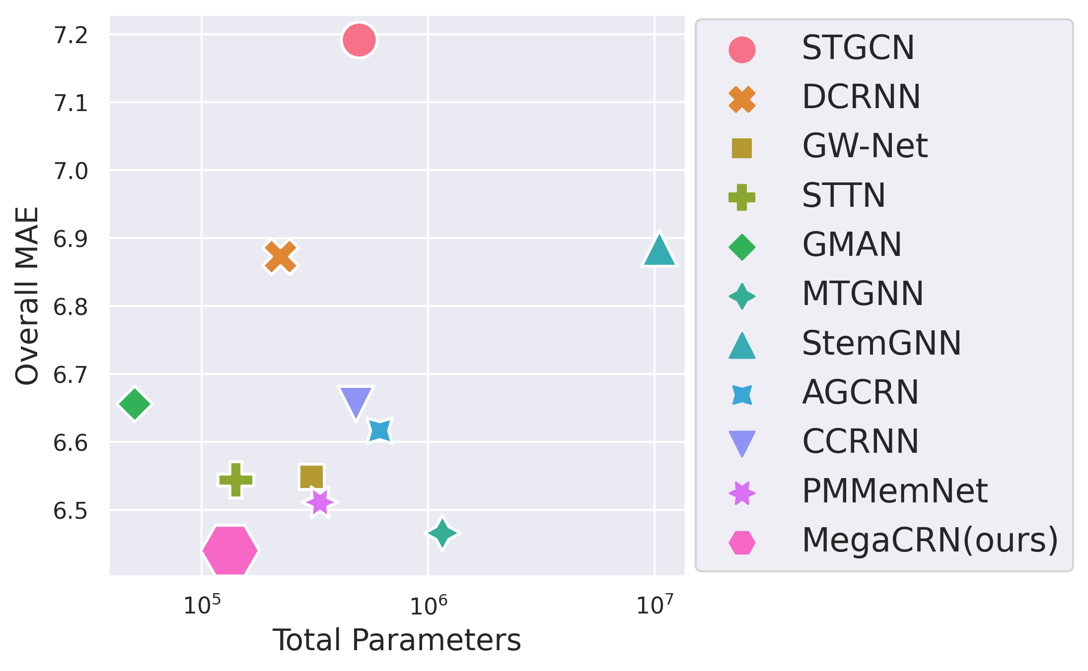
Figure 3: Efficiency Evaluation

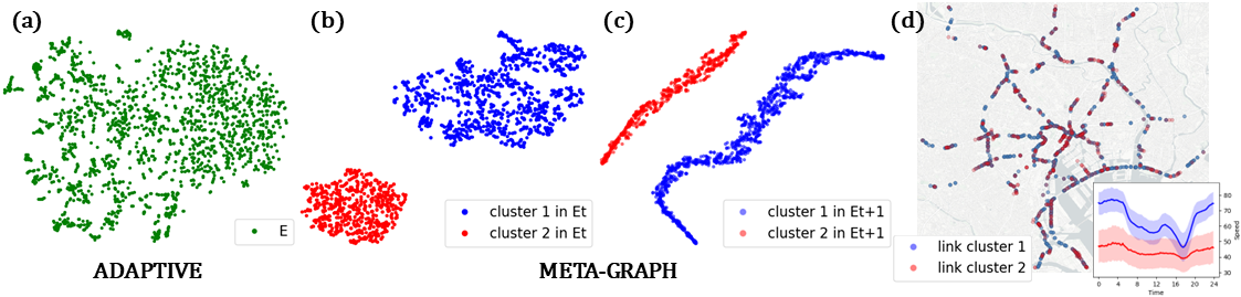
Figure 4: Spatio-Temporal Disentangling Effect of Meta-Graph Learning

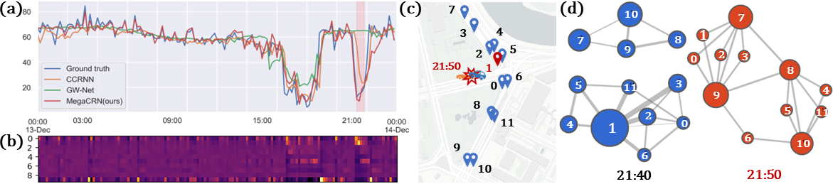
Figure 5: Incident Awareness of MegaCRN

Efficiency Study. We also evaluate the efficiency of our model by comparing with the-state-of-the-arts. Here we just report the results on EXPY-TKY, because the spatial domain of our data is 5$\sim$9 times larger than the benchmarks. A scatter plot is shown as Figure 3, where the x-axis of is the total number of parameters and the y-axis is the overall MAE. We can see that our model has the second-fewest parameters (merely 133,597) but the smallest overall MAE. For a large-scale dataset like EXPY-TKY, our model could be very memory-efficient. In contrast, some models, especially Transformer-based models including GMAN (Zheng et al. 2020) and STTN (Xu et al. 2020), are very memory/time-consuming due to the dot-product operation on big tensor. Although our model tends to need more epochs to converge, each round of training could be finished in very little time. To sum up, our model can achieve the state-of-the-art precision while keeping comparatively efficient.

Qualitative Evaluation

Spatio-Temporal Disentanglement. We qualitatively evaluate the quality of node embeddings by visualizing them in a low-dimensional space with t-SNE. Compared with adaptive GSL illustrated as Figure 4(a), meta-graph can automatically learn to cluster nodes (i.e., road links) as shown in Figure 4(b)(c). Interestingly, as time evolves from t to t+1, this clustering effect persists but the cluster shape changes, which confirms the spatio-temporal disentangling capability as well as the time-adaptability of our approach. In addition, we map out the physical locations of the road links in discovered clusters with different colors (cluster 1 in blue, cluster 2 in red) in Figure 4(d). We observe a strong correlation between the spatial distribution of cluster 2 (in red) and interchanges/toll gates. From the daily averaged time series plot in the bottom of Figure 4(d), we can clearly tell the inter-cluster difference. While road links in cluster 1 (in blue) share a strong rush hour pattern, the other cluster (in red) has a lower speed on average but higher variations, which is characterized by large amount of speed change near interchanges/toll gates. These observations validate the power of Meta-Graph Learner to explicitly distinguish spatio-temporal heterogeneity.

Incident-Awareness. We qualitatively study the robustness of MegaCRN to various traffic situations in Figure 5. Here we select an incident case that occurred at 21:50 at road link 1, marked in red in Figure 5(a), on December 13th, 2021. In terms of the prediction results (in 60-minute lead time), compared with two baselines, GW-Net (Wu et al. 2019) and CCRNN (Ye et al. 2021), our model can not only better capture normal fluctuations, but adapt to more complex situations including rush hour and traffic accident (in shaded red). Such sudden disturbance inevitably results in delay or failure of detection for other models. From the visualization of memory query weight in Figure 5(b), we can tell that the pattern querying to the Meta-Node Bank is different between normal situations and rush hour or incident case. This observation confirms the distinguishing power and generalizability to diverse traffic scenarios. We further visualize the learned local meta-graph as Figure 5(d), in which thicker line represents higher edge weight and bigger node size means larger weighted outdegree. Intuitively, we can find the meta-graph is changing with time. At 21:40 before the accident happened, node 1 (road link 1) held the biggest impact in the local meta-graph as road link 1 lies right at the center of the large road intersection. Then at 21:50 after the accident happened, the impact of node 1 dropped significantly and the graph became dominated by road link 7, 8, 9, and 10 that formed a separated subgraph at 21:40. This case study verifies the superior adaptability of our approach.

Conclusion

In this study, we propose Meta-Graph Convolutional Recurrent Network (MegaCRN) along with a novel spatio-temporal graph structure learning mechanism for traffic forecasting. Besides two benchmarks, METR-LA and PEMS-BAY, we further generate a brand-new traffic dataset called EXPY-TKY from large-scale car GPS records and collect the corresponding traffic incident information. Our model outperformed the state-of-the-arts to a large degree on all three datasets. Through a series of visualizations, it also demonstrated the capability to disentangle the time and nodes with different patterns as well as the adaptability to incident situations. We will further generalize our model for Multivariate Time Series forecasting tasks in the future.

References

- Bai et al. (2020) Bai, L.; Yao, L.; Li, C.; Wang, X.; and Wang, C. 2020. Adaptive graph convolutional recurrent network for traffic forecasting. Advances in Neural Information Processing Systems, 33: 17804–17815.
- Cao et al. (2020) Cao, D.; Wang, Y.; Duan, J.; Zhang, C.; Zhu, X.; Huang, C.; Tong, Y.; Xu, B.; Bai, J.; Tong, J.; et al. 2020. Spectral temporal graph neural network for multivariate time-series forecasting. Advances in Neural Information Processing Systems, 33: 17766–17778.
- Chung et al. (2014) Chung, J.; Gulcehre, C.; Cho, K.; and Bengio, Y. 2014. Empirical evaluation of gated recurrent neural networks on sequence modeling. arXiv preprint arXiv:1412.3555.
- Defferrard, Bresson, and Vandergheynst (2016) Defferrard, M.; Bresson, X.; and Vandergheynst, P. 2016. Convolutional neural networks on graphs with fast localized spectral filtering. In Advances in neural information processing systems, 3844–3852.
- Deng et al. (2021) Deng, J.; Chen, X.; Jiang, R.; Song, X.; and Tsang, I. W. 2021. ST-Norm: Spatial and Temporal Normalization for Multi-variate Time Series Forecasting. In Proceedings of the 27th ACM SIGKDD Conference on Knowledge Discovery & Data Mining, 269–278.
- Diao et al. (2019) Diao, Z.; Wang, X.; Zhang, D.; Liu, Y.; Xie, K.; and He, S. 2019. Dynamic spatial-temporal graph convolutional neural networks for traffic forecasting. In Proceedings of the AAAI conference on artificial intelligence, volume 33, 890–897.
- Ding et al. (2021) Ding, Y.; Yao, Q.; Zhao, H.; and Zhang, T. 2021. Diffmg: Differentiable meta graph search for heterogeneous graph neural networks. In Proceedings of the 27th ACM SIGKDD Conference on Knowledge Discovery & Data Mining, 279–288.
- Geng et al. (2019) Geng, X.; Li, Y.; Wang, L.; Zhang, L.; Yang, Q.; Ye, J.; and Liu, Y. 2019. Spatiotemporal multi-graph convolution network for ride-hailing demand forecasting. In Proceedings of the AAAI conference on artificial intelligence, volume 33, 3656–3663.
- Gong et al. (2019) Gong, D.; Liu, L.; Le, V.; Saha, B.; Mansour, M. R.; Venkatesh, S.; and Hengel, A. v. d. 2019. Memorizing normality to detect anomaly: Memory-augmented deep autoencoder for unsupervised anomaly detection. In Proceedings of the IEEE/CVF International Conference on Computer Vision, 1705–1714.
- Guo et al. (2019) Guo, S.; Lin, Y.; Feng, N.; Song, C.; and Wan, H. 2019. Attention based spatial-temporal graph convolutional networks for traffic flow forecasting. In Proceedings of the AAAI conference on artificial intelligence, volume 33, 922–929.
- Ha, Dai, and Le (2016) Ha, D.; Dai, A.; and Le, Q. V. 2016. Hypernetworks. arXiv preprint arXiv:1609.09106.
- Hamilton and Susmel (1994) Hamilton, J. D.; and Susmel, R. 1994. Autoregressive conditional heteroskedasticity and changes in regime. Journal of econometrics, 64(1-2): 307–333.
- Hochreiter and Schmidhuber (1997) Hochreiter, S.; and Schmidhuber, J. 1997. Long short-term memory. Neural computation, 9(8): 1735–1780.
- Huang et al. (2014) Huang, W.; Song, G.; Hong, H.; and Xie, K. 2014. Deep architecture for traffic flow prediction: Deep belief networks with multitask learning. Intelligent Transportation Systems, IEEE Transactions on, 15(5): 2191–2201.
- Jiang et al. (2021) Jiang, R.; Yin, D.; Wang, Z.; Wang, Y.; Deng, J.; Liu, H.; Cai, Z.; Deng, J.; Song, X.; and Shibasaki, R. 2021. DL-Traff: Survey and Benchmark of Deep Learning Models for Urban Traffic Prediction. In Proceedings of the 30th ACM International Conference on Information & Knowledge Management, 4515–4525.
- Jiang and Luo (2021) Jiang, W.; and Luo, J. 2021. Graph neural network for traffic forecasting: A survey. arXiv preprint arXiv:2101.11174.
- Kipf et al. (2018) Kipf, T.; Fetaya, E.; Wang, K.-C.; Welling, M.; and Zemel, R. 2018. Neural relational inference for interacting systems. In International Conference on Machine Learning, 2688–2697. PMLR.
- Kipf and Welling (2017) Kipf, T. N.; and Welling, M. 2017. Semi-Supervised Classification with Graph Convolutional Networks.
- Lai et al. (2018) Lai, G.; Chang, W.-C.; Yang, Y.; and Liu, H. 2018. Modeling long-and short-term temporal patterns with deep neural networks. In The 41st International ACM SIGIR Conference on Research & Development in Information Retrieval, 95–104.
- Lee et al. (2022) Lee, H.; Jin, S.; Chu, H.; Lim, H.; and Ko, S. 2022. Learning to Remember Patterns: Pattern Matching Memory Networks for Traffic Forecasting. In International Conference on Learning Representations.
- Li et al. (2021) Li, F.; Feng, J.; Yan, H.; Jin, G.; Jin, D.; and Li, Y. 2021. Dynamic graph convolutional recurrent network for traffic prediction: Benchmark and solution. arXiv preprint arXiv:2104.14917.
- Li et al. (2019) Li, S.; Jin, X.; Xuan, Y.; Zhou, X.; Chen, W.; Wang, Y.-X.; and Yan, X. 2019. Enhancing the locality and breaking the memory bottleneck of transformer on time series forecasting. Advances in Neural Information Processing Systems, 32.
- Li et al. (2018) Li, Y.; Yu, R.; Shahabi, C.; and Liu, Y. 2018. Diffusion Convolutional Recurrent Neural Network: Data-Driven Traffic Forecasting. In International Conference on Learning Representations.
- Lu et al. (2020) Lu, B.; Gan, X.; Jin, H.; Fu, L.; and Zhang, H. 2020. Spatiotemporal adaptive gated graph convolution network for urban traffic flow forecasting. In Proceedings of the 29th ACM International Conference on Information & Knowledge Management, 1025–1034.
- Lv et al. (2014) Lv, Y.; Duan, Y.; Kang, W.; Li, Z.; and Wang, F.-Y. 2014. Traffic flow prediction with big data: a deep learning approach. IEEE Transactions on Intelligent Transportation Systems, 16(2): 865–873.
- Lv et al. (2018) Lv, Z.; Xu, J.; Zheng, K.; Yin, H.; Zhao, P.; and Zhou, X. 2018. Lc-rnn: A deep learning model for traffic speed prediction. In IJCAI, volume 2018, 27th.
- Ma et al. (2015a) Ma, X.; Tao, Z.; Wang, Y.; Yu, H.; and Wang, Y. 2015a. Long short-term memory neural network for traffic speed prediction using remote microwave sensor data. Transportation Research Part C: Emerging Technologies, 54.
- Ma et al. (2015b) Ma, X.; Yu, H.; Wang, Y.; and Wang, Y. 2015b. Large-scale transportation network congestion evolution prediction using deep learning theory. PloS one, 10(3): e0119044.
- Oord et al. (2016) Oord, A. v. d.; Dieleman, S.; Zen, H.; Simonyan, K.; Vinyals, O.; Graves, A.; Kalchbrenner, N.; Senior, A.; and Kavukcuoglu, K. 2016. Wavenet: A generative model for raw audio. arXiv preprint arXiv:1609.03499.
- Pan, Demiryurek, and Shahabi (2012) Pan, B.; Demiryurek, U.; and Shahabi, C. 2012. Utilizing real-world transportation data for accurate traffic prediction. In 2012 ieee 12th international conference on data mining, 595–604. IEEE.
- Park, Noh, and Ham (2020) Park, H.; Noh, J.; and Ham, B. 2020. Learning memory-guided normality for anomaly detection. In Proceedings of the IEEE/CVF Conference on Computer Vision and Pattern Recognition, 14372–14381.
- Santoro et al. (2016) Santoro, A.; Bartunov, S.; Botvinick, M.; Wierstra, D.; and Lillicrap, T. 2016. Meta-learning with memory-augmented neural networks. In International conference on machine learning, 1842–1850. PMLR.
- Seo et al. (2018) Seo, Y.; Defferrard, M.; Vandergheynst, P.; and Bresson, X. 2018. Structured sequence modeling with graph convolutional recurrent networks. In International Conference on Neural Information Processing, 362–373. Springer.
- Shang, Chen, and Bi (2021) Shang, C.; Chen, J.; and Bi, J. 2021. Discrete Graph Structure Learning for Forecasting Multiple Time Series. In International Conference on Learning Representations.
- Shao et al. (2022) Shao, Z.; Zhang, Z.; Wang, F.; and Xu, Y. 2022. Pre-training Enhanced Spatial-temporal Graph Neural Network for Multivariate Time Series Forecasting. In Proceedings of the 28th ACM SIGKDD Conference on Knowledge Discovery and Data Mining, 1567–1577.
- Shih, Sun, and Lee (2019) Shih, S.-Y.; Sun, F.-K.; and Lee, H.-y. 2019. Temporal pattern attention for multivariate time series forecasting. Machine Learning, 108(8-9): 1421–1441.
- Stock and Watson (2001) Stock, J. H.; and Watson, M. W. 2001. Vector autoregressions. Journal of Economic perspectives, 15(4): 101–115.
- Vaswani et al. (2017) Vaswani, A.; Shazeer, N.; Parmar, N.; Uszkoreit, J.; Jones, L.; Gomez, A. N.; Kaiser, Ł.; and Polosukhin, I. 2017. Attention is all you need. Advances in neural information processing systems, 30.
- Veličković et al. (2017) Veličković, P.; Cucurull, G.; Casanova, A.; Romero, A.; Lio, P.; and Bengio, Y. 2017. Graph attention networks. arXiv preprint arXiv:1710.10903.
- Vinyals et al. (2016) Vinyals, O.; Blundell, C.; Lillicrap, T.; Wierstra, D.; et al. 2016. Matching networks for one shot learning. Advances in neural information processing systems, 29.
- Wang et al. (2020) Wang, X.; Ma, Y.; Wang, Y.; Jin, W.; Wang, X.; Tang, J.; Jia, C.; and Yu, J. 2020. Traffic flow prediction via spatial temporal graph neural network. In Proceedings of The Web Conference 2020, 1082–1092.
- Wang et al. (2022) Wang, Z.; Jiang, R.; Xue, H.; Salim, F. D.; Song, X.; and Shibasaki, R. 2022. Event-aware multimodal mobility nowcasting. In Proceedings of the AAAI Conference on Artificial Intelligence, volume 36, 4228–4236.
- Wu et al. (2020) Wu, Z.; Pan, S.; Long, G.; Jiang, J.; Chang, X.; and Zhang, C. 2020. Connecting the dots: Multivariate time series forecasting with graph neural networks. In Proceedings of the 26th ACM SIGKDD International Conference on Knowledge Discovery & Data Mining, 753–763.
- Wu et al. (2019) Wu, Z.; Pan, S.; Long, G.; Jiang, J.; and Zhang, C. 2019. Graph WaveNet for Deep Spatial-Temporal Graph Modeling. In IJCAI.
- Xu et al. (2021) Xu, J.; Wang, J.; Long, M.; et al. 2021. Autoformer: Decomposition transformers with auto-correlation for long-term series forecasting. Advances in Neural Information Processing Systems, 34.
- Xu et al. (2020) Xu, M.; Dai, W.; Liu, C.; Gao, X.; Lin, W.; Qi, G.-J.; and Xiong, H. 2020. Spatial-temporal transformer networks for traffic flow forecasting. arXiv preprint arXiv:2001.02908.
- Yao et al. (2019) Yao, H.; Liu, Y.; Wei, Y.; Tang, X.; and Li, Z. 2019. Learning from multiple cities: A meta-learning approach for spatial-temporal prediction. In The World Wide Web Conference, 2181–2191.
- Ye et al. (2021) Ye, J.; Sun, L.; Du, B.; Fu, Y.; and Xiong, H. 2021. Coupled Layer-wise Graph Convolution for Transportation Demand Prediction. In Proceedings of the AAAI Conference on Artificial Intelligence, volume 35, 4617–4625.
- Yu, Yin, and Zhu (2018) Yu, B.; Yin, H.; and Zhu, Z. 2018. Spatio-temporal graph convolutional networks: a deep learning framework for traffic forecasting. In Proceedings of the 27th International Joint Conference on Artificial Intelligence, 3634–3640.
- Yu and Koltun (2016) Yu, F.; and Koltun, V. 2016. Multi-Scale Context Aggregation by Dilated Convolutions. In ICLR.
- Zhang et al. (2020) Zhang, Q.; Chang, J.; Meng, G.; Xiang, S.; and Pan, C. 2020. Spatio-temporal graph structure learning for traffic forecasting. In Proceedings of the AAAI Conference on Artificial Intelligence, volume 34, 1177–1185.
- Zhang et al. (2021) Zhang, X.; Huang, C.; Xu, Y.; Xia, L.; Dai, P.; Bo, L.; Zhang, J.; and Zheng, Y. 2021. Traffic Flow Forecasting with Spatial-Temporal Graph Diffusion Network. In Proceedings of the AAAI Conference on Artificial Intelligence, volume 35, 15008–15015.
- Zhao et al. (2017) Zhao, H.; Yao, Q.; Li, J.; Song, Y.; and Lee, D. L. 2017. Meta-graph based recommendation fusion over heterogeneous information networks. In Proceedings of the 23rd ACM SIGKDD international conference on knowledge discovery and data mining, 635–644.
- Zhao et al. (2019) Zhao, L.; Song, Y.; Zhang, C.; Liu, Y.; Wang, P.; Lin, T.; Deng, M.; and Li, H. 2019. T-gcn: A temporal graph convolutional network for traffic prediction. IEEE Transactions on Intelligent Transportation Systems, 21(9): 3848–3858.
- Zheng et al. (2020) Zheng, C.; Fan, X.; Wang, C.; and Qi, J. 2020. Gman: A graph multi-attention network for traffic prediction. In Proceedings of the AAAI Conference on Artificial Intelligence, volume 34, 1234–1241.
- Zhou et al. (2021) Zhou, H.; Zhang, S.; Peng, J.; Zhang, S.; Li, J.; Xiong, H.; and Zhang, W. 2021. Informer: Beyond efficient transformer for long sequence time-series forecasting. In Proceedings of AAAI.
- Zhu et al. (2021) Zhu, Y.; Xu, W.; Zhang, J.; Liu, Q.; Wu, S.; and Wang, L. 2021. Deep graph structure learning for robust representations: A survey. arXiv preprint arXiv:2103.03036.