Radial Neighbors for Provably Accurate Scalable Approximations of Gaussian Processes

Abstract

In geostatistical problems with massive sample size, Gaussian processes (GP) can be approximated using sparse directed acyclic graphs to achieve scalable $O(n)$ computational complexity. In these models, data at each location are typically assumed conditionally dependent on a small set of parents which usually include a subset of the nearest neighbors. These methodologies often exhibit excellent empirical performance, but the lack of theoretical validation leads to unclear guidance in specifying the underlying graphical model and may result in sensitivity to graph choice. We address these issues by introducing radial neighbors Gaussian processes and corresponding theoretical guarantees. We propose to approximate GPs using a sparse directed acyclic graph in which a directed edge connects every location to all of its neighbors within a predetermined radius. Using our novel construction, we show that one can accurately approximate a Gaussian process in Wasserstein-2 distance, with an error rate determined by the approximation radius, the spatial covariance function, and the spatial dispersion of samples. Our method is also insensitive to specific graphical model choice. We offer further empirical validation of our approach via applications on simulated and real world data showing state-of-the-art performance in posterior inference of spatial random effects.

Keywords: Approximations; Directed acyclic graph; Gaussian process; Spatial statistics; Wasserstein distance.

1 Introduction

Data indexed by spatial coordinates are routinely collected in massive quantities due to the rapid pace of technological development in imaging sensors, wearables and tracking devices. Statistical models of spatially correlated data are most commonly built using Gaussian processes due to their flexibility and their ability to straightforwardly quantify uncertainty. Spatial dependence in the data is typically characterized by a parametric covariance function whose unknown parameters are estimated by repeatedly evaluating a multivariate normal density with a dense covariance matrix. At each density evaluation, the inverse covariance matrix and its determinant must be computed at a complexity that is cubic on the data dimension $n$. This steep cost severely restricts the applicability of Gaussian processes on modern geolocated datasets. This problem is exacerbated in Bayesian hierarchical models computed via Markov-chain Monte Carlo (MCMC) because several thousands of $O(n^{3})$ operations must be performed to fully characterize the joint posterior distribution.

A natural idea for retaining the flexibility of Gaussian processes while circumventing their computational bottlenecks is to use approximate methods for evaluating high dimensional multivariate Gaussian densities. If the scalable approximation is “good” in some sense, then one can use the approximate method for backing out inferences on the original process parameters. A multitude of such scalable methods has been proposed in the literature. Low-rank methods using inducing variables or knots (Quiñonero-Candela and Rasmussen, 2005; Cressie and Johannesson, 2008; Banerjee et al., 2008; Finley et al., 2009; Guhaniyogi et al., 2011; Sang et al., 2011) are only appropriate for approximating very smooth Gaussian processes because the number of inducing variables must increase polynomially fast with the sample size to avoid oversmoothing of the spatial surface (Stein, 2014; Burt et al., 2020). Scalability can also be achieved by assuming sparsity of the Gaussian covariance matrix via compactly supported covariance functions (Furrer et al., 2006; Kaufman et al., 2008; Bevilacqua et al., 2019); these methods operate by assuming marginal independence of pairs of data points that are beyond a certain distance from each other. See also the related method of Gramacy and Apley (2015). Using a similar intuition, one can achieve scalability by approximating the high dimensional Gaussian density with a product of small dimensional densities that characterize dependence of nearby data points. Composite likelihood methods (Bai et al., 2012; Eidsvik et al., 2014; Bevilacqua and Gaetan, 2015) approximate the high dimensional Gaussian density with the product of sub-likelihoods, whereas Gaussian Markov Random Fields (GMRF; Cressie, 1993; Rue and Held, 2005) approximate it via a product of conditional densities whose conditioning sets include all the local spatial neighbors.

Markovian conditional independence assumptions based on spatial neighborhoods can be visualized as a sparse undirected graphical model; these assumptions are intuitively appealing and lead to sparse precision (inverse covariance) matrices and more efficient computations (Rue, 2001). However, the normalizing constant of GMRF densities may require additional expensive computations, and additional approximation steps may be required when making predictions at new spatial locations because GMRFs do not necessarily extend to a standalone stochastic process. Both these problems can be resolved by ordering the data and conditioning only using previously ordered data points. Because one can now use a directed acyclic graph to represent conditional independence in the data, this approximation (due to Vecchia, 1988) immediately leads to a valid density which can be extended to a standalone stochastic process.

There is a rich literature on approximations of Gaussian processes using directed acyclic graphs. In addition to extensions of Vecchia’s method (Datta et al., 2016; Finley et al., 2019; Katzfuss and Guinness, 2021), scalable models can be built on domain partitions (Peruzzi et al., 2022), and generalizations are available for non-Gaussian and multivariate data (Zilber and Katzfuss, 2021; Peruzzi and Dunson, 2022b, a) as well as for modeling nonstationary processes (Jin et al., 2021; Kidd and Katzfuss, 2022). However, we identify two issues with current approaches based on Vecchia’s approximation. First, because the graphical model representation of Vecchia approximations is not unique, the numerical performance of these methods can be sensitive to the choice of graphical model in certain scenarios (Guinness, 2018). Including remote locations in the conditioning sets may be helpful (Stein et al., 2004), but there is no consensus on how to populate these conditioning sets. Second, although their performance has been demonstrated in practice (Heaton et al., 2019), there is a lack of theoretical support for Vecchia approximations of Gaussian process. The recent work by Schäfer et al. (2021) established Kullback-Leibler divergence bounds for Vecchia approximations, but under strong conditions that are difficult to verify for commonly used spatial covariance functions.

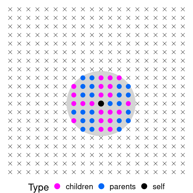
In this paper, we address these two issues by introducing a novel method and corresponding theoretical guarantees. Our radial neighbors Gaussian process (RadGP) scalably approximates a Gaussian process by assuming conditional independence at spatial locations as prescribed by a directed acyclic graph. A directed edge connects every location to all of its neighbors within a predetermined radius $\rho$. For this reason, our method is more closely related to GMRFs than other methods based on Vecchia approximations. Relative to GMRFs, our method allows to straightforwardly compute the Cholesky factor of the precision matrix, leading to computational advantages. Relative to Vecchia approximations, our method is by construction less sensitive to the choice of graphical model. Figure 1 visualizes how our proposed method differs from a typical Vecchia approximation construction.

We also introduce–to the best of our knowledge–the first general theoretical result regarding the closeness between a Vecchia-like method and the original Gaussian process it approximates. Our theory is readily applicable to popular spatial covariance functions such as the Matérn. We show that RadGP enables accurate approximations of Gaussian processes in Wasserstein-2 distance, with an error rate determined by the approximation radius, the spatial covariance function, and the spatial dispersion of samples. Empirical studies demonstrate our RadGP has similar performance in kriging and advantageous performance in posterior joint prediction tasks when compared to existing Vecchia approximation methods.

2 Radial Neighbors Gaussian process

2.1 Alternating partitions

Let the spatial domain $\Omega$ be a connected subset of $\mathbb{R}^{d}$. Let $Z=\{Z_{s}:s\in\Omega\}$ be a real valued Gaussian process on $\Omega$ with mean function $m:\Omega\to\mathbb{R}$ and covariance function $K:\Omega\times\Omega\to\mathbb{R}$ such that for all $s_{1},s_{2}\in\Omega$, $\mathbb{E}(Z_{s_{1}})=m(s_{1})$, and $\mathrm{Cov}(Z_{s_{1}},Z_{s_{2}})=K(s_{1},s_{2})$. Let $\{\mathcal{T}_{i}\}_{i\geq 1}$ be a countable sequence of disjoint spatial location sets and $\mathcal{D}=\cup_{i\geq 1}\mathcal{T}_{i}$. In practice, we regard the first set $\mathcal{T}_{1}$ as the training set, the second set $\mathcal{T}_{2}$ as the current test set, and all subsequent $\mathcal{T}_{i}$ with $i\geq 3$ as test sets that may arrive in the future. We assume that $\mathcal{D}$ includes all possible testing locations.

Let $\mathcal{P}=\{\mathcal{D}_{i}\}_{i\geq 1}$ be a countable disjoint partition of $\mathcal{D}$ such that $\cup_{i}\mathcal{D}_{i}=\mathcal{D}$. We refer to a partition $\mathcal{P}$ as an alternating partition of $\mathcal{D}$ with distance $\rho$ if for all $\mathcal{D}_{i}$ and $s\in\mathcal{D}_{i}$, we have $U(s,\rho)\cap(\mathcal{D}_{i}\backslash s)=\emptyset$, where $U(s,\rho)$ is the open ball centered at $s$ with Euclidean radius $\rho$. Basically, for an alternating partition $\mathcal{P}$, any two elements in the same subset $\mathcal{D}_{i}$ are at least $\rho$ distance away from each other. In the special case where $\mathcal{D}=\mathcal{T}_{1}$ and the elements of $\mathcal{T}_{1}$ are equally spaced locations in $\Omega$, an alternating partition can be intuitively understood as alternatively putting elements of $\mathcal{D}$ into several subsets. An example of an alternating partition in the 2-dimensional space with $\mathcal{D}=\mathcal{T}_{1}$ is shown in Fig. 1(d).

An alternating partition on $\mathcal{D}=\cup_{i\geq 1}\mathcal{T}_{i}$ can be computed in a sequential manner. We first compute a partition on the training set $\mathcal{T}_{1}$; then supposing a partition on $\cup_{j=1}^{i}\mathcal{T}_{i}$ is already known, we can expand it to incorporate the next testing set $\mathcal{T}_{i+1}$. The detailed steps are in Algorithm 1. Alternating partitions are often not unique and our algorithm provides a parsimonious solution with a relatively small number of partitioned subsets, as shown in Lemma 1.

Lemma 1.

Letting $\mathcal{P}=\{\mathcal{D}_{1},\ldots,\mathcal{D}_{M}\}$ be the final partition output from Algorithm 1 on $\mathcal{T}_{1},\ldots,\mathcal{T}_{M_{t}}$ sequentially, then the number of partitioned subsets $M$ satisfies $M\leq\sum_{k=1}^{M_{t}}\sup_{s\in\mathcal{T}_{k}}|U(s,\rho)\cap\mathcal{T}_{k}|,$ where $|\cdot|$ denotes the cardinality.

In the special case when the spatial locations in each $\mathcal{T}_{k}$ are $l^{d}$ equally spaced points in $[0,1]^{d}$ for a positive integer $l$, Lemma 1 implies that $M$ is roughly of the order $M_{t}\pi^{d/2}\Gamma^{-1}(d/2+1)\rho^{d}l^{d}$. Since a $d$-dimensional ball with radius $\rho/2$ covers about $\pi^{d/2}\Gamma^{-1}(d/2+1)(\rho/2)^{d}l^{d}$ grid points of $\mathcal{D}$ and any two points in this ball belong to two different subsets in the alternating partition, the result of Lemma 1 is optimal up to a constant multiplier $2^{d}M_{t}$.

(a) Maximal distance between a location and its parents.

(b) Parent and child set of Vecchia GP.

(c) Parent and child set of RadGP.

(d) Alternating partitions and $\rho$ radius for the first three layers $\mathcal{D}_{1}$, $\mathcal{D}_{2}$ and $\mathcal{D}_{3}$ on grid training set $T_{1}$.

Figure 1: Graph structures of RadGP and Vecchia approximations with maximin ordering. In (a), the x-axis for each curve is the order used by the corresponding Cholesky of the precision matrix.

Input a new spatial location set $\mathcal{T}_{i}$ and the existing partition $\mathcal{P}=\{\mathcal{D}_{1},\ldots,\mathcal{D}_{M}\}$. For the training set $\mathcal{T}_{1}$, the existing partition is set to be $\mathcal{P}=\{\emptyset\}$.

Let $A_{1}=\mathcal{T}_{i}$ be the set of elements waiting to be assigned and $A_{2}=\emptyset$ be the subset of $A_{1}$ whose elements are within Euclidean distance $\rho$ of some locations that have already been assigned. Let $m=M$.

while $A_{1}\neq\emptyset$ do

       Randomly select $s\in A_{1}$. Let $A_{1}=A_{1}\backslash\{s\}$ and $A_{2}=A_{1}\cap U(s,\rho)\backslash\{s\}$.

       For all $m\leq i\leq M$, compute the minimum distance $\rho_{i}$ between $s$ and $\mathcal{D}_{i}$. Let $j=\min\{j:m\leq j\leq M,\rho_{j}\geq\rho\}$. Assign $s$ to subset $j$ by setting $\mathcal{D}_{j}=\mathcal{D}_{j}\cup\{s\}$.

       while $A_{2}\neq\emptyset$ do

             Randomly select $s\in A_{2}$. Let $A_{1}=A_{1}\backslash\{s\}$ and $A_{2}=A_{2}\cup(A_{1}\cap U(s,\rho))\backslash\{s\}$.

             for $s^{\prime}\in U(s,\rho)$ do

                   For all $m\leq i\leq M$, compute the minimum distance between $s^{\prime}$ and $\mathcal{D}_{i}$ as $\rho_{i}$.

                   if $\max\{\rho_{i}:m\leq i\leq M\}<\rho$ then

                         Assign $s^{\prime}$ to a new subset, by setting $M=M+1$, $\mathcal{D}_{M}=\{s^{\prime}\}$.

                  else

                         Let $j=\min\{j:m\leq j\leq M,\rho_{j}\geq\rho\}$. Assign $s^{\prime}$ to subset $j$: $\mathcal{D}_{j}=\mathcal{D}_{j}\cup\{s^{\prime}\}$.

                        

                   end if

                  

             end for

            

       end while

      

end while

Result: Output the updated partition $\mathcal{P}=\{\mathcal{D}_{1},\ldots,\mathcal{D}_{M}\}$.

Algorithm 1 Alternating Partition for a New Spatial Location Set $\mathcal{T}_{i}$.

2.2 Radial neighbors directed acyclic graphs

We now define a directed acyclic graph based on the alternating partition output by Algorithm 1. Specifically, Let $\mathcal{P}=\{\mathcal{D}_{i}\}_{i\geq 1}$ be an alternating partition on $\mathcal{D}=\cup_{i\geq 1}\mathcal{T}_{i}$. Order elements in $\mathcal{D}$ as $\mathcal{D}=\{w_{1},w_{2},\cdots\}$ such that if $w_{i}\in\mathcal{D}_{i_{d}}$, $w_{j}\in\mathcal{D}_{j_{d}}$ and $i_{d}<j_{d}$, then $i<j$. Then, the directed acyclic graph on $\mathcal{D}$ is defined in the following way: (1) For all $i_{d}\geq j_{d}$, there are no directed edges from elements in $\mathcal{D}_{i_{d}}$ to elements in $\mathcal{D}_{j_{d}}$; (2) For all $i_{d}<j_{d}$, all $w_{i}\in\mathcal{D}_{i_{d}}$ and $w_{j}\in\mathcal{D}_{j_{d}}$, there is a directed edge from $w_{i}$ to $w_{j}$ if and only if their Euclidean distance $\|w_{i}-w_{j}\|_{2}<\rho$; (3) For all $w_{i}\in\mathcal{D}_{1}$ with $i\geq 2$, if $w_{j}$ is the spatial location closest to $w_{i}$ among all locations with index $j$ smaller than $i$, then there is a directed edge from $w_{j}$ to $w_{i}$.

We name this directed acyclic graph as a radial neighbors graph because it ensures that for all locations $w_{i}\in\mathcal{D}$, any location within $\rho$ distance of $w_{i}$ has either a directed edge from $w_{i}$ or a directed edge to $w_{i}$. Our radial neighbors graph is less sensitive to the ordering of locations, because any Gaussian process built on a directed graph with this radial property is guaranteed to approximate the original Gaussian process.

2.3 Gaussian processes from radial neighbors graphs

We build our radial neighbors Gaussian process on $\mathcal{D}=\{w_{1},w_{2},\ldots\}$ using the directed graph defined via alternating partitions, in which each $w_{i}$ is conditionally only dependent on its parent set. Let the symbol $\overset{d}{=}$ denote equality in distribution and define $\Sigma_{A,B}$ as the covariance matrix between two spatial location sets $A$ and $B$ under the covariance function $K(\cdot,\cdot)$. The conditional distribution of $\hat{Z}_{w_{i}}$ is defined as

$$[\hat{Z}_{w_{i}}\mid\hat{Z}_{w_{j}},j<i] \overset{d}{=}[\hat{Z}_{w_{i}}\mid\hat{Z}_{\mathrm{pa}(w_{i})}]\overset{d}{=}[{Z}_{w_{i}}\mid{Z}_{\mathrm{pa}(w_{i})}]$$

$$\sim N\Big{(}m(w_{i})+\Sigma_{\mathrm{pa}(w_{i}),w_{i}}^{\mathrm{\scriptscriptstyle T}}\Sigma_{\mathrm{pa}(w_{i}),~{}\mathrm{pa}(w_{i})}^{-1}[\hat{Z}_{\mathrm{pa}(w_{i})}-m\{\mathrm{pa}(w_{i})\}],$$

$$\quad\qquad K(w_{i},w_{i})-\Sigma_{\mathrm{pa}(w_{i}),w_{i}}^{\mathrm{\scriptscriptstyle T}}\Sigma_{\mathrm{pa}(w_{i}),~{}\mathrm{pa}(w_{i})}^{-1}\Sigma_{\mathrm{pa}(w_{i}),w_{i}}\Big{)},$$ (1)

where for $i=1$ the parent set $\mathrm{pa}(w_{1})$ is empty.

Equation (2.3) defines the distribution of $\hat{Z}$ on all finite subsets of $\mathcal{D}$. We then extend this process $\hat{Z}$ to arbitrary finite subsets of the whole space $\Omega$. For all $s\in\Omega\backslash\mathcal{D}$, we define the parents of $s$ as $\mathrm{pa}(s)=\{s^{\prime}\in\mathcal{T}_{1}:\|s^{\prime}-s\|_{2}<\rho\}$ where $\mathcal{T}_{1}$ is the training set. For any finite set $U\subset\Omega\backslash\mathcal{D}$, we define the conditional distribution of $\hat{Z}_{U}$ given $\hat{Z}_{\mathcal{T}_{1}}$ as

$$p(\hat{Z}_{U}\mid\hat{Z}_{\mathcal{T}_{1}}) =\prod_{s\in U}p(\hat{Z}_{s}\mid\hat{Z}_{\mathrm{pa}(s)})=\prod_{s\in U}p({Z}_{s}\mid Z_{\mathrm{pa}(s)}),$$

$$[\hat{Z}_{s}\mid\hat{Z}_{\mathrm{pa}(s)}] \sim N\Big{(}m(s)+\Sigma_{\mathrm{pa}(s),s}^{\mathrm{\scriptscriptstyle T}}\Sigma_{\mathrm{pa}(s),\mathrm{pa}(s)}^{-1}[\hat{Z}_{\mathrm{pa}(s)}-m\{\mathrm{pa}(s)\}],$$

$$\qquad\qquad K(s,s)-\Sigma_{\mathrm{pa}(s),s}^{\mathrm{\scriptscriptstyle T}}\Sigma_{\mathrm{pa}(s),\mathrm{pa}(s)}^{-1}\Sigma_{\mathrm{pa}(s),s}\Big{)}.$$ (2)

Equations (2.3) and (2.3) together give the joint distribution of $\hat{Z}$ on any finite subset of $\Omega$. Specifically, for a generic finite set $A=U\cup V$ with $U\subset\Omega\backslash\mathcal{D}$ and $V\subset\mathcal{D}$, we let $I=\max\{i\in\mathbb{N}:w_{i}\in V\}$ and define the finite $S$ as $S=(\{w_{i}:i\leq I\}\cup\mathcal{T}_{1})\backslash V$. Intuitively, $S$ is the collection of locations that are parent nodes for locations in $A$ but not included in $A$. The joint density of $\hat{Z}$ on $A$ implied by Equations (2.3) and (2.3) is

$$p(\hat{Z}_{A})=\int p(\hat{Z}_{U}|\hat{Z}_{\mathcal{T}_{1}})\prod_{s\in S\cup V}p(\hat{Z}_{s}|\hat{Z}_{\mathrm{pa}(s)})\prod_{s\in S}ds.$$ (3)

Equations (2.3)-(3) complete the definition of our radial neighbors Gaussian process.

Lemma 2.

The radial neighbors Gaussian process (RadGP) $\hat{Z}(\cdot)$ is a valid Gaussian process on the whole spatial domain $\Omega$.

The proof of Lemma 2 relies on the Kolmogorov extension theorem and is in the Supplementary Material.

3 Theoretical Properties

3.1 Wasserstein distances between Gaussian processes

Let $\mathcal{D}^{\prime}$ be a finite subset of the countable set $\mathcal{D}$ such that for all $s\in\mathcal{D}^{\prime}$, its parent set satisfies $\mathrm{pa}(s)\subset\mathcal{D}^{\prime}$. With a slight abuse of notation, we denote the elements of set $\mathcal{D}^{\prime}$ as $\mathcal{D}^{\prime}=\{w_{1},\ldots,w_{n}\}$ such that each node is always ordered before its child nodes. The objective of this section is to establish theoretical upper bounds for the Wasserstein distance between the original Gaussian process and the radial neighbors Gaussian process on all such finite subsets $\mathcal{D}^{\prime}$. For two generic random vectors $Z_{1},Z_{2}$ defined on the same space $\mathcal{Z}$ following the probability distributions $\mu_{1},\mu_{2}$, their Wasserstein-2 ($W_{2}$) distance is

$$W_{2}(Z_{1},Z_{2})=\left\{\min_{\tilde{\mu}\in\mathcal{M}}\int_{\mathcal{Z}\times\mathcal{Z}}\|z_{1}-z_{2}\|_{2}^{2}d\tilde{\mu}(z_{1},z_{2})\right\}^{1/2},$$

where $\mathcal{M}$ is the set of all probability distributions on the product space $\mathcal{Z}\times\mathcal{Z}$ whose marginals are $\mu_{1}$ and $\mu_{2}$. Let $Z_{\mathcal{D}^{\prime}}$ and $\hat{Z}_{\mathcal{D}^{\prime}}$ be the random vectors from the original Gaussian process and the radial neighbors Gaussian process on the set $\mathcal{D}^{\prime}$. Denote the covariance matrix of $Z_{\mathcal{D}^{\prime}}$ and $\hat{Z}_{\mathcal{D}^{\prime}}$ as $\Sigma_{\mathcal{D}^{\prime}\mathcal{D}^{\prime}}$ and $\hat{\Sigma}_{\mathcal{D}^{\prime}\mathcal{D}^{\prime}}$, the precision matrix of $Z_{\mathcal{D}^{\prime}}$ and $\hat{Z}_{\mathcal{D}^{\prime}}$ as $\Sigma_{\mathcal{D}^{\prime}\mathcal{D}^{\prime}}^{-1}$ and $\hat{\Phi}$, respectively. Then the Wasserstein-2 distance between $Z_{\mathcal{D}^{\prime}}$ and $\hat{Z}_{\mathcal{D}^{\prime}}$ has a closed form (Gelbrich, 1990):

$$W_{2}^{2}(Z_{\mathcal{D}^{\prime}},\hat{Z}_{\mathcal{D}^{\prime}})=\mathrm{tr}(\Sigma_{\mathcal{D}^{\prime}\mathcal{D}^{\prime}})+\mathrm{tr}(\hat{\Sigma}_{\mathcal{D}^{\prime}\mathcal{D}^{\prime}})-2\mathrm{tr}\{(\Sigma_{\mathcal{D}^{\prime}\mathcal{D}^{\prime}}^{1/2}\hat{\Sigma}_{\mathcal{D}^{\prime}\mathcal{D}^{\prime}}\Sigma_{\mathcal{D}^{\prime}\mathcal{D}^{\prime}}^{1/2})^{1/2}\},$$ (4)

where $\mathrm{tr}(A)$ denotes the trace of a square matrix $A$. The right-hand side of equation (4) involves various matrix powers that are difficult to analyze. Fortunately, for Gaussian measures, the squared Wasserstein-2 distance can be upper bounded by the trace norm of the difference between their covariance matrices. As shown in Lemma S2 of the Supplementary Material, our radial neighbors Gaussian process induces a Cholesky decomposition of the precision matrix, which further upper bounds the Wasserstein-2 distance with column norms of Cholesky factors. Specifically, let a decomposition of $\Sigma_{\mathcal{D}^{\prime}\mathcal{D}^{\prime}}^{-1}$ be $\Sigma_{\mathcal{D}^{\prime}\mathcal{D}^{\prime}}^{-1}=LL^{T}$ with $L=(l_{1},\ldots,l_{n})$; similarly let $\hat{\Phi}=\hat{L}\hat{L}^{T}$ with $\hat{L}=(\hat{l}_{1},\ldots,\hat{l}_{n})$. For a generic $m\times m$ symmetric matrix $A$, let $\lambda_{\max}(A)$ be its largest eigenvalue. For a generic $k\times m$ matrix $B$, let $\|B\|_{2}=\{\lambda_{\max}(B^{{\mathrm{\scriptscriptstyle T}}}B)\}^{1/2}$ and $\|B\|_{\mathrm{tr}}=\mathrm{tr}\{(B^{{\mathrm{\scriptscriptstyle T}}}B)^{1/2}\}$.

Lemma 3.

For any decomposition $\Sigma_{\mathcal{D}^{\prime}\mathcal{D}^{\prime}}^{-1}=LL^{\mathrm{\scriptscriptstyle T}}$ and $\hat{{\Phi}}=\hat{L}\hat{L}^{\mathrm{\scriptscriptstyle T}}$, if $\|\hat{L}-L\|_{2}\leq\|\Sigma_{\mathcal{D}^{\prime}\mathcal{D}^{\prime}}\|_{2}^{-1/2}/2$, then we have

$$W_{2}^{2}(Z_{\mathcal{D}^{\prime}},\hat{Z}_{\mathcal{D}^{\prime}}) \leq\|\Sigma_{\mathcal{D}^{\prime}\mathcal{D}^{\prime}}-\hat{\Sigma}_{\mathcal{D}^{\prime}\mathcal{D}^{\prime}}\|_{\mathrm{tr}}$$

$$\leq 8n\|\Sigma_{\mathcal{D}^{\prime}\mathcal{D}^{\prime}}\|_{2}^{2}\big{(}2\max_{i}\|{l}_{i}\|_{2}\max_{i}\|{l}_{i}-\hat{{l}}_{i}\|_{2}+\max_{i}\|{l}_{i}-\hat{{l}}_{i}\|_{2}^{2}\big{)}.$$

Lemma 3 shows the difference between the two covariances in the trace norm depends on the cardinality of set $\mathcal{D}^{\prime}$, the covariance matrix of $Z_{\mathcal{D}^{\prime}}$ and the difference between ${l}_{i}$ and $\hat{{l}}_{i}$. Next, we will show that the matrix norms of $\Sigma_{\mathcal{D}^{\prime}\mathcal{D}^{\prime}}$, $l_{i}$ and $\hat{{l}}_{i}$ in Lemma 3 are dependent on the decay rate of covariance function $K(\cdot,\cdot)$ and minimal separation distance in the set $\mathcal{D}^{\prime}$.

3.2 Spatial decaying families

We consider the Gaussian process $Z=(Z_{s}:s\in\Omega)$ with mean zero and an isotropic nonnegative covariance function $K(\cdot,\cdot)$. Thus we can reformulate $K$ as $K(s_{1},s_{2})=K_{0}(\|s_{1}-s_{2}\|_{2})$ for any $s_{1},s_{2}\in\Omega$, where $K_{0}:[0,+\infty)\to[0,+\infty)$. For all $r>0$, define the function $v_{r}(\cdot):\mathbb{R}\to\mathbb{R}_{+}$ as $v_{r}(x)=\sum_{k=0}^{+\infty}|x|^{k}/(k!)^{r}$. Then $1/v_{r}(x)$ is a monotone decreasing function of $x$, where a larger $r$ results in a slower decay rate in $1/v_{r}(x)$. Specifically, $1/v_{1}(x)=\exp(-x)$ and $1/v_{r}(x)$ with $r>1$ has a decay rate faster than all polynomials but slower than the exponential function. We also define a series of polynomials $c_{r}(x)=1+x^{r}$ for $r>0$. For each $v_{r}$ with $r>1$ and each $c_{r}$ with $r>0$, we define the following families of Gaussian processes:

$$\mathscr{Z}_{v_{r}} =\left\{Z=(Z_{s}:s\in\Omega):K_{0}(\|s_{1}-s_{2}\|_{2})\leq\frac{1}{v_{r}(\|s_{1}-s_{2}\|_{2})(1+\|s_{1}-s_{2}\|_{2}^{d+1})}\right\},$$ (5)

$$\mathscr{Z}_{c_{r}} =\left\{Z=(Z_{s}:s\in\Omega):K_{0}(\|s_{1}-s_{2}\|_{2})\leq\frac{1}{(1+\|s_{1}-s_{2}\|_{2})^{r}}\right\}.$$ (6)

Intuitively, $\mathscr{Z}_{v_{r}}$ is the family of isotropic Gaussian processes whose covariance function decays no slower than some subexponential rate of the spatial distance, while $\mathscr{Z}_{v_{r}}$ is the family with covariance functions decaying no slower than an $r$th order polynomial of the spatial distance.

The objective of our theoretical study is to bound the Wasserstein-2 distance between the marginal distribution of RadGP and original Gaussian process on $\mathcal{D}^{\prime}$ when the original process belongs to the two spatial decaying families in (5) and (6):

$$\sup_{Z\in\mathscr{Z}_{v_{r}}}W^{2}_{2}(Z_{\mathcal{D}^{\prime}},\hat{Z}_{\mathcal{D}^{\prime}})\quad\text{and}\quad\sup_{Z\in\mathscr{Z}_{c_{r}}}W^{2}_{2}(Z_{\mathcal{D}^{\prime}},\hat{Z}_{\mathcal{D}^{\prime}}).$$ (7)

As shown in Lemma 3, the above Wasserstein-2 distance can be controlled by some matrix norms multiplying the $l_{2}$ norm of ${l}_{i}-\hat{{l}}_{i}$. According to Lemma S2 of the Supplementary Material, ${l}_{i}$ and $\hat{{l}}_{i}$ differ in the sense that ${l}_{i}$ is computed using $\{w_{j}:j<i\}$, the set of all locations ordered before the $i$th location, while $\hat{{l}}_{i}$ is computed using $\{w_{j}:j<i,\|w_{j}-w_{i}\|_{2}<\rho\}$, a subset of locations that is within $\rho$ distance to the $i$th location. If we can show there are spatial decaying patterns on the set $\{w_{j}:j<i\}$ for various matrix quantities including the covariance matrices, the precision matrices and their Choleksy factors, then we can control the impact from those remote locations on the $i$th location, which allows the difference between $l_{i}$ and $\hat{l}_{i}$ to be controlled.

Specifically, let the matrix $A\in\mathbb{R}^{n\times n}$ be associated with $n$ spatial locations $w_{1},\ldots,w_{n}$ such that the $(i,j)$-entry of $A$, denoted by $A[i,j]$, is a function of the difference $w_{i}-w_{j}$. Let $w_{i}[l]$ be the $l$th coordinate of $w_{i}$. For all $1\leq l\leq d$, define a linear matrix operator $\nabla_{l}$ such that $\nabla_{l}({A})[i,j]=\big{(}w_{i}[l]-w_{j}[l]\big{)}{A}[i,j]$. For such a square matrix $A$, we define its $l$th order $v_{r}$ norm and $c_{r}$ norm as $\|{A}\|_{v_{r},l}=\sum_{k=0}^{+\infty}\|\nabla_{l}^{k}({A})\|_{2}/\{(k!)^{r}\}$ and $\|{A}\|_{c_{r}}=\left\{\sum_{k\in\mathbb{Z}^{d}}\sup_{w_{i},w_{j}\in\mathcal{D}^{\prime}}({A}[i,j])^{2}(1+\|w_{i}-w_{j}\|_{\infty})^{2r}\mathbbm{1}_{\{w_{i}-w_{j}\in[0,1)^{d}+k\}}\right\}^{1/2}$, which are related to the functions $v_{r}$ and $c_{r}$ defined above. These two matrix norms describe the spatial decaying properties in the sense that if a matrix $A$ has a finite $\|\cdot\|_{v_{r},l}$ norm (or $\|\cdot\|_{c_{r}}$ norm), then its $(i,j)$-entry decays at the rate $1/v_{r}(\|w_{i}-w_{j}\|_{\infty})$ (or $1/c_{r}(\|w_{i}-w_{j}\|_{\infty})$). By assuming the original Gaussian process coming from either $\mathscr{Z}_{v_{r},l}$ or $\mathscr{Z}_{c_{r}}$, we immediately obtain the spatial decaying patterns for covariance matrices. To obtain such patterns for their precision matrices and Cholesky factors, we need a tool known as the theory of norm-controlled inversion, developed by Gröchenig and Klotz (2014) and Fang and Shin (2020). The following lemma leverages the norm-controlled inversion theory to control the inverse matrix in $v_{r}$ and $c_{r}$ norms:

Lemma 4.

Let ${A}\in n\times n$ be an invertible matrix. If $\|A\|_{v_{r},l}<\infty$ for some $r>1$ and all $1\leq l\leq d$, then $\|{A}^{-1}\|_{v_{r},l}\leq\|{A}^{-1}\|_{2}v_{r-1}(\|{A}^{-1}\|_{2}\|{A}\|_{v_{r},l})$. If $\|\cdot\|_{c_{r}}<\infty$ for some $r\geq d+1$, then there exist positive constants $c_{4},c_{5}$ only dependent on the dimension $d$, such that $\|{A}^{-1}\|_{c_{r}}\leq c_{4}c_{5}^{r}\{\max(1,1/q)\}^{6d}\|{A}^{-1}\|_{2}\big{(}\|{A}^{-1}\|_{2}\|{A}\|_{c_{r}}\big{)}^{r+d/2}.$

Lemma 4 states a very strong result: if a matrix $A$ has some spatial decaying properties, such as its entries decaying like the function $1/v_{r}$ or $1/c_{r}$, then its inverse matrix also inherits such spatial decaying properties. Using this lemma on the covariance matrix and its principal submatrices, we can show in Lemma S2 and S3 of the Supplementary Material that the $l_{2}$ norm of $l_{i}-\hat{l}_{i}$ can be bounded in terms of the order $r$ and the spatial distances among $\mathcal{D}^{\prime}$.

3.3 Rate of approximation

For the countable set $\mathcal{D}^{\prime}$ described above, we define the minimal separation distance among all spatial locations in $\mathcal{D}^{\prime}$ as $q=\min_{1\leq i<j\leq|\mathcal{D}^{\prime}|}\|w_{i}-w_{j}\|_{2}$. This minimal separation distance is a parsimonious statistic for describing the spatial dispersion of $\mathcal{D}^{\prime}$, and is useful in bounding various quantities such as the maximal eigenvalue and condition number of $\Sigma_{\mathcal{D}^{\prime}\mathcal{D}^{\prime}}$; see Lemma S1 of the Supplementary Material. Let $\hat{K}_{0}(w)=(2\pi)^{-d/2}\int K_{0}(x)\exp(-\imath w^{{\mathrm{\scriptscriptstyle T}}}x)dx$ be the Fourier transform of $K_{0}$ where $\imath^{2}=-1$, and let $\phi_{0}(x)=\inf_{\|w\|_{2}\leq 2x}\hat{K}_{0}(w)$ for all $x>0$. For two positive sequences $a_{n}$ and $b_{n}$, we use $a_{n}\lesssim b_{n}$ to denote the relation $\lim_{n\to\infty}a_{n}/b_{n}$ is upper bounded by a constant that only depends on the dimension $d$. We have the following theorems on the Wasserstein-2 distance between the radial neighbors Gaussian process and the original Gaussian process. The constants $c_{1},c_{2}$ are from Lemma S1 while $c_{3}$ is from Lemma S2 in the Supplementary Material, all of which only depend on $d$.

Theorem 1.

Let $\mathcal{D}^{\prime}$ be defined as in Section 3.1. For the family $\mathscr{Z}_{v_{r}}$ in (5) with $r>1$, if $0<q<1$ and $n^{1/2}\{v_{r}(\rho d^{-1/2})\}^{-1}\{\phi_{0}(c_{2}/q)\}^{-9/2}v_{r-1}[c_{3}\{\phi_{0}(c_{2}/q)\}^{-1}]\leq c_{6}$ hold for some constant $c_{6}$ only dependent on $d$, then

$$\sup_{Z\in\mathscr{Z}_{v_{r}}}W_{2}^{2}(Z_{\mathcal{D}^{\prime}},\hat{Z}_{\mathcal{D}^{\prime}})\lesssim\frac{n}{v_{r}(\rho d^{-1/2})}\{\phi_{0}(c_{2}/q)\}^{-5}q^{-d}v_{r-1}[c_{3}\{\phi_{0}(c_{2}/q)\}^{-1}],$$

Else if $q\geq 1$ and $n^{1/2}/v_{r}(\rho d^{-1/2})\leq c^{\prime}_{6}$ hold for some constant $c^{\prime}_{6}$ only dependent on $d$, then $\sup_{Z\in\mathscr{Z}_{v_{r}}}W^{2}_{2}(Z_{\mathcal{D}^{\prime}},\hat{Z}_{\mathcal{D}^{\prime}})\lesssim n/v_{r}(\rho d^{-1/2}).$

Theorem 2.

Let $\mathcal{D}^{\prime}$ be defined as in Section 3.1. For the family $\mathscr{Z}_{c_{r}}$ in (6) with $r\geq d+1$, if $0<q<1$ and $n^{1/2}(1+\rho d^{-1/2})^{-(r-d-1)}q^{(r-7)d}\{\phi_{0}(c_{2}/q)\}^{-(r+4)}(c_{1}c_{5}d2^{d-1}\pi/\surd{6})^{r}\leq c_{7}$ hold for some constant $c_{7}$ only dependent on $d$, then

$$\sup_{Z\in\mathscr{Z}_{c_{r}}}W_{2}^{2}(Z_{\mathcal{D}^{\prime}},\hat{Z}_{\mathcal{D}^{\prime}})\lesssim\frac{n}{(1+\rho d^{-1/2})^{r-d-1}}q^{(r-8)d}\{\phi_{0}(c_{2}/q)\}^{-(r+9/2)}(c_{1}c_{5}d2^{d-1}\pi/\surd{6})^{r},$$

Else if $q\geq 1$ and $n^{1/2}(1+\rho d^{-1/2})^{-(r-d-1)}\{\phi_{0}(c_{2}/q)\}^{-r}(c_{1}c_{5}d2^{d-1}\pi/\surd{6})^{r}\leq c^{\prime}_{7}$ hold for some constant $c^{\prime}_{7}$ only dependent on $d$, then $\sup_{Z\in\mathscr{Z}_{c_{r}}}W^{2}_{2}(Z_{\mathcal{D}^{\prime}},\hat{Z}_{\mathcal{D}^{\prime}})\lesssim$ $n(1+\rho d^{-1/2})^{-(r-d-1)}$ $\{\phi_{0}(c_{2}/q)\}^{-r}(c_{1}c_{5}d2^{d-1}\pi/\surd{6})^{r}.$

The conditions for the above theorems, namely the equations regarding $c_{6},c^{\prime}_{6},c_{7},c^{\prime}_{7}$, are necessary but not sufficient conditions for the upper bounds of Wasserstein-2 distance to go to zero. Thus, they can be safely ignored if we aim for accurate approximations. We now give a detailed analysis of these upper bounds for Wasserstein-2 distance, which involves three variables: the sample size $n$, the minimal separation distance $q$, and the approximation radius $\rho$ in the radial neighbors Gaussian process.

First, the upper bounds in Theorems 1 and 2 are linearly dependent on the sample size $n$. This is tight in the situation where the domain $\Omega$ grows with the sample size $n$ while both the minimal separation distance $q$ and the approximation radius $\rho$ are fixed, corresponding to the increasing domain asymptotics regime in the spatial literature. As $n$ increases, the local structure for existing locations will not change and the approximation accuracy for them will not improve. Thus more locations will lead to a linearly increasing approximation error in the $W_{2}$ distance.

Second, the upper bounds on the squared $W_{2}$ distance decay with respect to the approximation radius $\rho d^{-1/2}$ at the same rate as the spatial covariance function with respect to the spatial distance, up to a $(d+1)$th order polynomial. For Theorem 1, the covariance function is required to decay faster than $1/v_{r}(x)$ by a polynomial $1+x^{d+1}$ as defined in equation (5); for Theorem 2, the covariance function decays faster than an $r$th order polynomial while the upper bound of $W_{2}$ distance decays at an $(r-d-1)$th order polynomial. Such $(d+1)$th polynomials in Theorems 1 and 2 come from the fact that high dimension reduces the effective decay rate of covariance function. For example, under a fixed minimal separation distance, when $d=1$, as long as the covariance function decays faster than $1/x$ by a polynomial term, the matrix $\Sigma_{\mathcal{D}^{\prime}\mathcal{D}^{\prime}}$ has a bounded $l_{1}$ norm regardless of sample size; however, for a general $d$ dimensional space, the covariance function must decay faster than $1/x^{d}$ for $\Sigma_{\mathcal{D}^{\prime}\mathcal{D}^{\prime}}$ to have a bounded $l_{1}$ norm. These upper bounds show that the approximation radius $\rho$ indeed controls the approximation accuracy. Specifically, since the squared $W_{2}$ distance upper bounds the sum of squared errors, for a fixed minimal separation distance $q$, we can reach an arbitrarily small mean squared error uniformly for all $n\in\mathbb{N}$ by increasing $\rho$ over some threshold value; see our detailed conditions on $\rho$ in Corollary 1 for various types of covariance functions.

Third, both upper bounds in the two theorems increase with respect to the minimal separation distance $q$. This is because as the minimal separation distance decreases, spatial locations get closer to each other and the covariance matrix gets close to singular, which requires a larger approximation radius to compensate.

We now apply our theorems to Gaussian processes with various covariance functions that are commonly used in the spatial literature. The specification of covariance functions enables more concrete evaluation of the Fourier transform $\phi_{0}(\cdot)$ and therefore, further leads to explicit evaluation of the required approximation radius $\rho$ to make the Wasserstein-2 distances in Theorems 1 and 2 converge to zero.

Corollary 1.

We have $W_{2}^{2}(Z_{\mathcal{D}^{\prime}},\hat{Z}_{\mathcal{D}^{\prime}})\to 0$ as $n\to\infty$ if one of the following conditions is satisfied: (1) The covariance function is the isotropic Matérn: $K_{0}(s_{1}-s_{2})=\sigma^{2}2^{1-\nu}{\Gamma(\nu)}^{-1}\left(\alpha\|s_{1}-s_{2}\|\right)^{\nu}\mathcal{K}_{\nu}\left(\alpha\|s_{1}-s_{2}\|_{2}\right)$ with $q<1/\alpha$. Define the constant $c_{m,1}=\Gamma(\nu)/\{\sigma^{2}2^{d}\pi^{d/2}\Gamma(\nu+d/2)\}$. The approximation radius $\rho$ satisfies

$$\rho\geq\frac{d^{1/2}}{\alpha}\left[c_{3}c_{m,1}\Big{(}1+\frac{4c_{2}^{2}}{\alpha^{2}q^{2}}\Big{)}^{\nu+\frac{d}{2}}+\ln\Big{\{}c_{m,1}nq^{-d}\Big{(}1+\frac{4c_{2}^{2}}{\alpha^{2}q^{2}}\Big{)}^{5(\nu+\frac{d}{2})}\Big{\}}\right]^{3}.$$

(2) The covariance function is Gaussian $K_{0}(\|s_{1}-s_{2}\|_{2})=\sigma^{2}\exp(-a\|s_{1}-s_{2}\|_{2}^{2})$ with $q<a^{-1/2}$. The approximation radius $\rho$ satisfies

$$\rho\geq\left(\frac{d}{a}\right)^{1/2}\left[c_{3}\sigma^{-2}\exp\big{\{}c_{2}^{2}/(aq^{2})\big{\}}+\ln(nq^{-d}\sigma^{-10})+\frac{5c_{2}^{2}}{aq^{2}}\right]^{3}.$$

(3) The covariance function is the generalized Cauchy $K_{0}(\|s_{1}-s_{2}\|_{2})=\sigma^{2}\big{\{}1+(\|s_{1}-s_{2}\|/\alpha)^{\delta}\big{\}}^{-\lambda/\delta}$ with parameter $\lambda>d+1$ and $q<\alpha$. Let $c_{9}$ be a constant dependent on dimension $d$ and covariance function parameters $\sigma^{2},\alpha,\delta,\lambda$. The approximation radius $\rho$ satisfies

$$\rho\geq c_{9}q^{-\frac{\frac{25}{2}d+\delta(\lambda+\frac{9}{2})}{\lambda-(d+1)}}n^{\frac{1}{\lambda-(d+1)}}.$$

Corollary 1 presents the concrete relations between the approximation radius $\rho$, the minimal separation distance $q$, and the sample size $n$ that are sufficient to achieve vanishing approximation error in the squared Wasserstein-2 distance. Specifically, for a fixed $q$, when the covariance function decays faster than any polynomial, which includes Matérn in case (1) and Gaussian in case (2) of Corollary 1, the approximation radius $\rho$ only needs to grow very slowly in the order $O(\ln^{3}n)$, which is much smaller than the full data size $n$. On the other hand, if the covariance function decays only at a polynomial rate such as the generalized Cauchy in case (3) of Corollary 1, the approximation radius $\rho$ also needs to grow at a polynomial rate of $n$ as well. This is understandable because for covariance functions that decrease slowly in the spatial distance, one needs more spatial locations and a larger approximation radius to capture the dependence information and accurately approximate the distribution on the whole dataset.

Another implication of Corollary 1 is that the radius $\rho$ needs to be greater than some functions of $1/q$. Such functions are polynomials of $1/q$ when the covariance function is either Matérn or generalized Cauchy, but an exponenial function of $1/q$ when the covariance function is Gaussian. This is mainly due to the limitation of spatially decaying family $\mathscr{Z}_{v_{r}}$ in (5) we have used. In order to have nice norm-controlled inversion properties, the spatial decaying rate of covariance functions in $\mathscr{Z}_{v_{r}}$ need to be slower than exponential, that is, with $r>1$ in $v_{r}(x)$, while the Gaussian covariance function decays much faster than $1/v_{r}(x)$. Thus, the condition required for the case (2) in Corollary 1 on Gaussian is not necessarily the tightest.

Our results fill a major gap in the literature by providing the previously lacking theoretical support for popular local or neighborhood-based Gaussian process approximations. Our theory only requires knowledge of the spatial decaying pattern of the covariance functions (e.g., exponential and polynomial in $\mathscr{Z}_{v_{r}}$ and $\mathscr{Z}_{c_{r}}$, respectively). These conditions are easily verifiable, with derivations for the Matérn, Gaussian and the generalized Cauchy covariance functions provided in Corollary 1. Similar techniques can be used for a wider range of stationary covariance functions. Furthermore, our novel theory explicitly links the approximation quality from choosing radius $\rho$ with the minimal separation distance $q$ and the sample size $n$, both of which are readily available from observed data.

4 Bayesian Regression with RadGP

Consider a linear regression model with spatial latent effects as:

$$Y(s)=X(s)\beta+Z(s)+\epsilon(s),\;s\in\Omega,$$ (8)

where $X(s)$ are covariates at location $s$, $\beta$ are regression coefficients for the covariates, $Z(s)$ is a Gaussian process with zero mean and covariance function $K_{\theta}:\Omega\times\Omega\to\mathbb{D}$, and $\epsilon(s)$ is a white noise process. Researchers observe $Y(s),X(s)$ at a collection of training locations $\mathcal{T}_{1}$ with the objective of estimating the regression coefficients $\beta$, the covariance function parameters $\theta$, and the spatial random effects $Z(s)$ at both training locations $\mathcal{T}_{1}$ and test locations $\mathcal{T}_{2}\subset\Omega$. If the spatial random effects $Z(s)$ are not of interest, one can combine $Z(s)$ and $\epsilon(s)$ into one Gaussian process, known as the response model. This is described in Section S5 of the Supplementary Material. Hereafter we assume that inference on $Z(s)$ is desired. Let $Z_{\mathcal{T}_{1}}$ denote the column vector consisting of $\{Z(s):s\in\mathcal{T}_{1}\}$. Similarly define other notation with $\mathcal{T}_{i}$ as subscripts. Endowing the spatial random effects with our radial neighbors Gaussian process prior, the full Bayesian model can be outlined as follows:

$$(\beta,\theta,\sigma)\sim p(\beta)p(\theta)p(\sigma),\quad\epsilon(s)\overset{\text{i.i.d.}}{\sim}N(0,\sigma^{2}),s\in\Omega,\quad\hat{Z}_{\mathcal{T}_{1}}|\theta\sim N(0,\hat{\Phi}^{-1}),$$

$$p(\hat{Z}_{\mathcal{T}_{2}}|\hat{Z}_{\mathcal{T}_{1}},\theta)\propto\prod_{k=1}^{M}\prod_{s\in\mathcal{T}_{2}\cap\mathcal{D}_{k}}p(\hat{Z}_{s}|\hat{Z}_{\mathrm{pa}(s)}),\quad Y(s)=X(s)\beta+\hat{Z}(s)+\epsilon(s),$$ (9)

where the radial neighbors precision matrix $\hat{\Phi}$ and $p(\hat{Z}_{s}|\hat{Z}_{\mathrm{pa}(s)})$ are defined in equation (2.3). The priors for $\beta,\theta$ and $\sigma$ can be flexible, but it is advised to set a proper prior for either $\sigma$ or $\theta$ due to potential non-identifiability.

We employ a Gibbs sampling framework while handling each full conditional with different approaches. If the prior of $\beta$ is normal $\beta\sim N(\beta_{0},\Phi_{0}^{-1})$, then the posterior of $\beta$ is also normal:

$$\beta|{Y}_{\mathcal{T}_{1}},\hat{Z}_{\mathcal{T}_{1}},\sigma^{2}$$

$$\sim N\big{(}(\Phi_{0}+{X}_{\mathcal{T}_{1}}^{T}{X}_{\mathcal{T}_{1}}/\sigma^{2})^{-1}\{\Phi_{0}\beta_{0}+{X}_{\mathcal{T}_{1}}^{T}({Y}_{\mathcal{T}_{1}}-\hat{Z}_{\mathcal{T}_{1}})/\sigma^{2}\},(\Phi_{0}+{X}_{\mathcal{T}_{1}}^{T}{X}_{\mathcal{T}_{1}}/\sigma^{2})^{-1}\big{)}.$$ (10)

We then sample $\sigma$ from its full conditional. If the prior distribution for $\sigma^{2}$ is inverse gamma $\sigma^{2}\sim\mathrm{IG}(a_{0},b_{0})$, then the posterior of $\sigma^{2}$ is also inverse gamma:

$$\sigma^{2}|{Y}_{\mathcal{T}_{1}},\hat{Z}_{\mathcal{T}_{1}},\beta\sim\mathrm{IG}\left(a_{0}+n/2,b_{0}+\|{Y}_{\mathcal{T}_{1}}-{X}_{\mathcal{T}_{1}}\beta-\hat{Z}_{\mathcal{T}_{1}}\|_{2}^{2}/2\right).$$ (11)

We sample the spatial random effects on $\mathcal{T}_{1}$ with conjugate gradients as illustrated in Nishimura and Suchard (2022), using the full conditional distribution:

$$\hat{Z}_{\mathcal{T}_{1}}|{Y}_{\mathcal{T}_{1}},\beta,\sigma^{2},\theta\sim N({\xi},(\hat{\Phi}+{I}_{n}/\sigma^{2})^{-1}),$$

where ${\xi}=(\hat{{\Phi}}+{I}_{n}/\sigma^{2})^{-1}({Y}_{\mathcal{T}_{1}}-{X}_{\mathcal{T}_{1}}\beta)/\sigma^{2}$.

Finally, for Gaussian process parameter $\theta$, there is no available conjugate prior in general. We sample $\theta$ using Metropolis Hasting relying on full conditional $p(\theta|\hat{Z}_{\mathcal{T}_{1}})\propto p(\hat{Z}_{\mathcal{T}_{1}}|\theta)p(\theta)$. The computation of density $p(\hat{Z}_{\mathcal{T}_{1}}|\theta)$ can be decomposed into the computation of $n$ conditional densities, all of which can be computed in parallel given $\hat{Z}_{\mathcal{T}_{1}}$. A detailed algorithm for posterior sampling can be found in Section S5.1 of the Supplementary Material.

If prediction on a test set is of interest, given MCMC samples of random effects on training set $\mathcal{T}_{1}$ and parameter $\theta$, $Z_{\mathcal{T}_{2}}$ can be sampled from each unidimensional Gaussian distribution as in equation (9). Unlike most previous related work, this prediction accounts for dependence among test locations, which is important in many applied contexts. For example, instead of just wanting to obtain separate marginal predictions at each spatial location, one may want to predict some functional of the set of values in a particular spatial region, such as the variance or maximum.

Under a fixed minimal separation distance, the computational complexity for both training and testing is linear in their respective sample size. Specifically, for training, the major computational complexity comes from sampling random effects via solving linear systems with conjugate gradients. The number of conjugate gradient steps is dependent on the condition number of the precision matrix, while the time for each step is dependent on the number of nonzero elements of the precision matrix. The former is a constant while the later is linear in sample size. For testing, it is only required to sample $|\mathcal{T}_{2}|$ unidimensional Gaussian random variables, which has time complexity $O(|\mathcal{T}_{2}|M^{3})$, where $M$ is the number of partitioned subsets in Lemma 1.

The above posterior inference framework can easily accommodate sequential datasets. Specifically, if we receive dataset $\mathcal{T}_{3}$ after finishing training on $\mathcal{T}_{1}$ and testing on $\mathcal{T}_{2}$, we can extend the alternating partition and directed graph to $\mathcal{T}_{3}$ without changing the graph structures on $\mathcal{T}_{i},i\leq 2$. Thus the posterior inference on $\mathcal{T}_{3}$ can be done without retraining the model and takes only an incremental computational complexity of $O(|\mathcal{T}_{3}|M^{3})$.

5 Experimental Studies

5.1 Simulation Studies

We study the performance of radial neighbors Gaussian processes for the spatial regression model (8) with no covariates, where the true model for spatial effects $Z(s)$ is a Gaussian process with zero mean and exponential covariance function $K_{0}(x)=\tau^{2}\exp(-\phi x)$. The model parameters are $\phi,\tau^{2}$ and nugget variance $\sigma^{2}$, all of which are unknown and need to be estimated from training data. We set the true parameter values as $(\phi_{0},\tau_{0},\sigma_{0})=(19.97,1,0.1)$. The value $\phi_{0}=19.97$ is obtained by setting $K_{0}(0.15)=0.05$, a choice previously used by Katzfuss et al. (2020). The value $\sigma_{0}=0.1$ ensures the nugget is not too large compared to the spatial process. We set priors as $p(\phi)\propto 1$, $\tau^{2}\sim\mathrm{IG}(2,1)$, $\sigma^{2}\sim\mathrm{IG}(2,0.01)$. The domain is set as $\Omega=[0,1]^{2}$, with training data consisting of $1600$ grid locations in $\Omega$. We replicate the analysis on 50 datasets. For each dataset, the test set is generated as $1000$ i.i.d. uniformly distributed samples in $\Omega$.

Three methods are compared: RadGP proposed in this paper, nearest-neighbor Gaussian process (NNGP) (Datta et al., 2016) with maximin ordering and Vecchia Gaussian process predictions (V-Pred) (Katzfuss et al., 2020) with maximin ordering. The last two methods share the same training procedure while differing in prediction procedures: Datta et al. (2016) assumes that testing locations are independent given training locations while Katzfuss et al. (2020) allows dependencies among testing locations. For the tuning parameters, we set $\rho=0.055$ for RadGP and neighbor size $8$ for the other two methods. These parameters are set to ensure the total time of training and testing are roughly equal among the three methods.

We assess performances using a variety of metrics including posterior mean of parameters, mean squared error and coverage of $95\%$ credible intervals. Table 1 shows the mean and $90\%$ confidence intervals obtained over the $50$ replicated datasets. We can see that all methods achieve accurate estimation of the covariance parameters $\phi,\tau^{2}$ while having a wide confidence interval for the nugget variance $\sigma^{2}$. The coverage of predictive intervals are also close to $0.95$ for all methods. Overall, radial neighbors Gaussian process achieves comparable performance with the other two state-of-the-art methods.

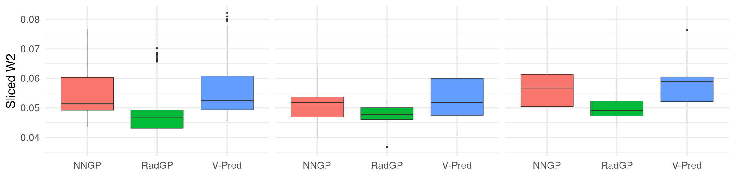
We are also interested in inferring dependence among test locations. Specifically, define $9$ local regions in $\Omega$ as $\mathscr{A}=\left\{A_{i}\times A_{j}:A_{i},A_{j}\in\{[0.15,0.25],[0.45,0.55],[0.75,0.85]\}\right\}$. We are interested in jointly predicting on test locations in each local region, with performance measured by the Wasserstein-2 distance between posterior predictive samples for these test locations and predictive samples generated from the true model. Since each region contains multiple locations and high-dimensional Wasserstein distances are difficult to compute, we instead use the sliced Wasserstein-2 distance (Bonneel et al., 2015), which is based on taking many projections of the high-dimensional distribution into a single dimension, and then integrating the unidimensional Wasserstein-2 distance with respect to the projection directions. In practice, this integration is approximated by Monte Carlo methods. As shown in Fig. 2, our method displays better performance in terms of the sliced Wasserstein-2 distance. This suggests that we obtain a more accurate approximation to the joint predictive distribution.

	Truth	RadGP	NNGP	V-Pred
$\phi$	19.97	20.45 (16.86, 23.27)	20.52 (17.02, 23.77)	-
$\tau^{2}$	1	0.998 (0.870, 1.115)	1.002 (0.877, 1.137)	-
$\sigma^{2}\times 10^{3}$	10	6.290 (1.398, 18.22)	4.287 (1.507, 10.50)	-
MSE	-	0.219 (0.196, 0.236)	0.219 (0.197, 0.235)	0.219 (0.197, 0.236)
coverage	0.9	0.951 (0.935, 0.967)	0.952 (0.936, 0.963)	0.952 (0.935, 0.963)
ave. time	-	4.344 sec	4.458 sec	4.404 sec

Table 1: Basic simulation performance for the RadGP, NNGP and the V-Pred modification of NNGP to account for predictive dependence. NNGP and V-Pred only differ in prediction.

Figure 2: Assessment of performance in joint prediction for the RadGP, NNGP and V-Pred methods on local regions $[0.15,0.25]\times[0.15,0.25]$, $[0.15,0.25]\times[0.45,0.55]$ and $[0.15,0.25]\times[0.75,0.85]$. We use sliced Wasserstein-2 distance to measure predictive accuracy.

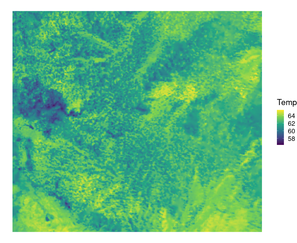
5.2 Surface Temperature Data

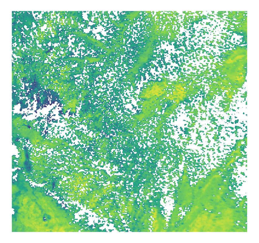
We consider the land surface temperature data on a $499\mathrm{km}\times 581\mathrm{km}$ region southeast of Addis Ababa in Ethiopia at April 1st, 2020. The data are a product of the MODIS (Moderate Resolution Imaging Spectroradiometer) instrument on the Aqua satellite. The original data set comes as a $499\times 581$ image with each pixel corresponding to a $1\mathrm{km}\times 1\mathrm{km}$ spatial region, as shown in Fig. 4 left. However, atmosphere conditions like clouds can block earth surfaces, resulting in missing data for many pixels. There are at $211,683$ spatial locations with observed temperature values and $78,236$ locations with missing values. We randomly split the training data into $3$ folds, using two folds for training and one fold for out-of-sample validation. This results in a total of $141,122$ training locations and $148,797$ testing locations.

We consider the same Gaussian process regression model as Section 5.1 with no covariates, zero mean function and exponential covariance function $K_{0}(x)=\tau^{2}\exp(-\phi x)$. The observed temperature values are centered to compensate for the lack of intercept term. We evaluate the performances of radial neighbors Gaussian process with radius $4.01\mathrm{km}$ and nearest neighbor Gaussian process with neighbor size $15$. The priors for both methods are set as $p(\phi)\propto 1$, $\tau^{2}\sim\mathrm{IG}(2,1)$ and $\sigma^{2}\sim\mathrm{IG}(1,0.1)$. Estimates for covariance parameters, out-of-sample mean squared errors and coverage for $95\%$ credible intervals are shown in Table 2. The results are quite similar between the two methods.

The observed temperature and predicted temperature are visualized in Fig. 4. In general, the land surface temperature changes smoothly with respect to geological locations. The east and south part of the figure, which is covered by less vegetation, features slightly higher surface temperature. Small variations of temperature also occur in many local regions, indicating the geographical complexity of Ethiopia. There is a small blue plate in the west border of the figure that has significantly lower surface temperature than its surroundings, which corresponds to several lakes in the Great Rift Valley.

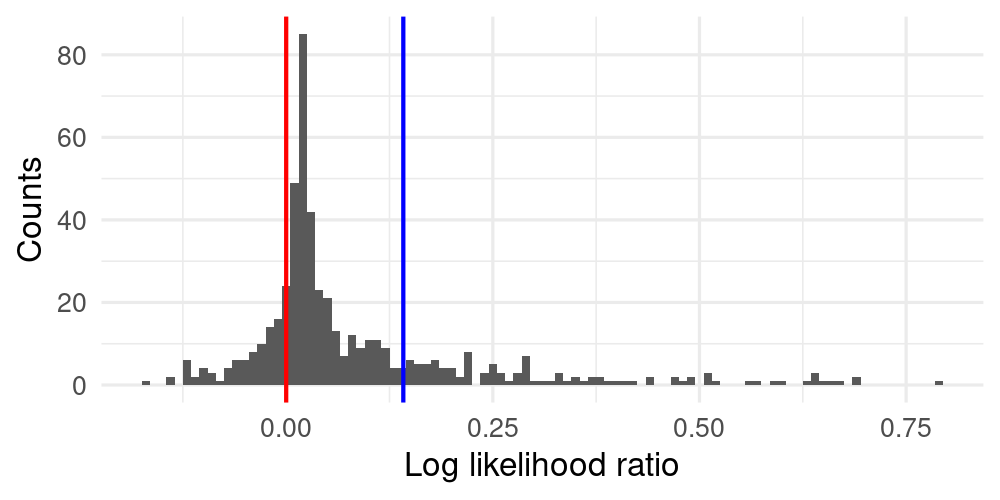
We further compare the performance of the two methods in terms of joint predictions at multiple held out locations. As we do not know the ground truth, we cannot calculate Wasserstein-2 error and instead focus on the joint likelihood ratio for held out data. Specifically, we select $567$ pairs of locations in the set reserved for out-of-sample validation. Each pair consists of two locations with $1$km distance from each other. Any two locations from different pairs are at least $10$km apart. For each pair of locations, we compute the logarithm of the likelihood ratio between RadGP and NNGP. The distribution of the log likelihood ratio can provide important information about joint inference. Specifically, the mean of the log likelihood ratio is $0.142$ and there are $78\%$ pairs with positive log likelihood ratios. Since the distribution of the log likelihood ratio has heavy tails with minimum $-1.361$ and maximum $6.531$, we remove the bottom and top $5\%$ of the values and visualize the rest in Fig. 3, where the red vertical line is $\mathrm{ratio}=0$. We can see in the majority of cases, RadGP performs better than NNGP in terms of characterizing dependencies between temperature at two close locations.

	RadGP	NNGP
$\phi$	0.056 (0.053, 0.059)	0.055 (0.049, 0.061)
$\tau^{2}$	1.739 (1.651, 1.826)	1.797 (1.613, 2.036)
$\sigma^{2}\times 10^{4}$	7.248 (6.622, 7.976)	6.978 (6.423, 7.715)
MSE	0.077	0.078
coverage	0.950	0.951
time	2661 sec	2398 sec

Table 2: Performance of RadGP and NNGP on
land surface temperature data.

Figure 3: Histogram of log likelihood ratio between RadGP and NNGP. The blue and red lines correspond to the mean log likelihood ratio value, and zero, respectively.

Figure 4: Ethiopian land surface temperature on April 1st, 2020. Left: observed data; Right: predicted values from RadGP.

6 Discussion

Vecchia approximations are arguably one of the most popular approaches for scaling up Gaussian process models to large datasets in spatial statistics. The major contribution of this article is to propose the first Vecchia-like approximation method that has strong theoretical guarantees in quantifying the accuracy of approximation to the original process. Our numerical experiments have shown competitive performance from the proposed RadGP compared to other Vecchia approximation methods. We have demonstrated that our method leads to improvements in characterizing joint predictive distributions while matching the performance of state-of-the-art methods in parameter estimation and marginal predictions.

Our current theory leads to several potential future research directions. First, we have established upper bounds for the approximation error to the original Gaussian process in Wasserstein-2 distance. We can further study lower bounds of this approximation error within specific families of approximations. It will be helpful to examine when the norm-controlled inversion bounds we have used in the proofs are tight, and whether the derived conditions on the approximation radius $\rho$ for various covariance functions in Corollary 1 can be made optimal for such families.

Second, existing Vecchia approximations that use maximin ordering (Katzfuss et al., 2020) systematically generate remote locations across the domain. While our theory shows close locations are effective in quantifying spatial dependence, it is still unclear whether and how remote locations help with the approximation of covariance function. We would like to expand our research into general Vecchia approximations. The objective is to study the approximation error for different approximation approaches and discover the optimal strategy that minimizes the approximation error under certain sparsity constraints.

Third, although our main focus has been on approximation of Gaussian processes, we can further consider how the approximate process will affect posterior estimation of model parameters, including spatial fixed effects and covariance parameters. Under our current theoretical framework, since the minimal separation distance $q$ needs to be lower bounded, we can study Bayesian parameter estimation under increasing domain (Mardia and Marshall, 1984) or mixed domain (Lahiri and Zhu, 2006) asymptotic regimes. It remains an open problem whether our scalable approximation can maintain posterior consistency and optimal rates for all model parameters. We leave these directions for future exploration.

Supplementary material

Proofs of lemmas, theorems and corollaries are available at Supplementary Material for “Radial Neighbors for Provably Accurate Scalable Approximations of Gaussian Processes.” An R package for regression models using radial neighbor Gaussian processes is available at https://github.com/mkln/radgp.

Supplementary Material for “Radial Neighbors for Provably Accurate Scalable Approximations of Gaussian Processes”

This supplementary material is organized as follows. Section S1 includes the proofs of lemmas in Section 2 of the main paper. Section S2 includes the proofs of lemmas in Section 3 of the main paper. Section S3 provides several auxiliary lemmas and their proofs. Section S4 includes the proofs of Theorems 1 and 2 and Corollary 1 in the main paper. Section S5 provides the posterior sampling algorithms for the RadGP regression model used in Section 4 of the main paper.

We define some notation that will be used throughout this supplementary material. The notation that is only used for specific lemmas will be defined before or in those lemmas. Let $\Omega$ be the spatial domain that is a connected subspace of $\mathbb{R}^{d}$. Let $Z=\{Z_{s}:s\in\Omega\}$ be a real valued Gaussian process on $\Omega$ with zero mean and covariance function $K:\Omega\times\Omega\to\mathbb{R}$ and let $\hat{Z}$ be the radial neighborhood Gaussian process (RadGP) on $\Omega$. Let $\{\mathcal{T}_{i}\}_{i\geq 1}$ be a countable sequence of disjoint spatial location sets and let their union be $\mathcal{D}=\cup_{i\geq 1}\mathcal{T}_{i}$. Let $\mathcal{P}=\{\mathcal{D}_{i}\}_{i\geq 1}$ be a countable disjoint partition of $\mathcal{D}$ such that $\cup_{i\geq 1}\mathcal{D}_{i}=\mathcal{D}$. We order the elements of $\mathcal{D}$ as $\mathcal{D}=\{w_{1},w_{2},\ldots\}$. For any index $i\in\mathbb{N}$, let $\nu(i)=\{j\in\mathbb{N}:j<i\}$ be the collection of indices that are smaller than $i$. Since $\Omega$ can be an uncountable set, we use $s$ to denote a generic spatial location of $\Omega$. In the context where a directed graph exists, we use $\mathrm{pa}(s)$ to denote the parent set of $s$. Finally, let $\mathcal{D}^{\prime}$ be a finite subset of $\mathcal{D}$ such that for all $s\in\mathcal{D}^{\prime}$, $\mathrm{pa}(s)\subset\mathcal{D}^{\prime}$. The set $\mathcal{D}^{\prime}$ will be the main focus of our theoretical studies.

For a finite set $A\subset\Omega$, let $Z_{A}$ be the finite-dimensional random variable of the process $Z$ on $A$. For two finite sets $A,B\subset\Omega$, we denote the covariance matrix between $Z_{A}$ and $Z_{B}$ as $\Sigma_{AB}$. For a generic square matrix $A$, let $\lambda_{\min}(A)$ and $\lambda_{\max}(A)$ be its smallest and largest eigenvalues. The matrix $l_{1}$, $l_{2}$ and trace norms are denoted by $\|\cdot\|_{1}$, $\|\cdot\|_{2}$ and $\|\cdot\|_{\mathrm{tr}}$. The vector $l_{1}$ and $l_{2}$ norms are denoted using the same notation as the matrix norms. Finally, for simplicity, we denote $(\hat{\Sigma}_{\mathcal{D}^{\prime}\mathcal{D}^{\prime}})^{-1}$ as $\hat{\Phi}$.

S1 Proofs of Lemmas in Section 2

S1.1 Proof of Lemma 1

Proof.

Without loss of generality, we can set any $T_{k}$ to be an empty set. Hence, it suffices to prove that, given an alternating partition $\mathcal{P}_{0}=\{D_{1},\ldots,\mathcal{D}_{M_{0}}\}$ on $\mathcal{T}_{1},\ldots,\mathcal{T}_{k}$, for a new set $\mathcal{T}_{k+1}$, the new partition $\mathcal{P}=\{\mathcal{D}_{1},\ldots,\mathcal{D}_{M}\}$ satisfies

$$M\leq M_{0}+\sup_{s\in\mathcal{T}_{k+1}}|U(s,\rho)\cap T_{k+1}|.$$

With a little abuse of notation, we denote the spatial locations in $\mathcal{T}_{k+1}$ as $\mathcal{T}_{k+1}=\{s_{1},\ldots,s_{n}\}$. The first location $s_{1}$ is either assigned to the $M_{0}$th subset or the $(M_{0}+1)$th subset. Thus $M\leq M_{0}+1\leq M_{0}+\sup_{s\in\mathcal{T}_{k+1}}|U(s,\rho)\cap T_{k+1}|$ after assigning $s_{1}$. Now we show by induction that $M\leq M_{0}+1\leq M_{0}+\sup_{s\in\mathcal{T}_{k+1}}|U(s,\rho)\cap T_{k+1}|$ holds after assigning $s_{1},\ldots,s_{i}$, for all $1\leq i\leq n$.

Suppose we have finished assigning the first $i$ locations in $\mathcal{T}_{k+1}$ with $M$ satisfying the induction assumption. Now consider the $(i+1)$th location $s_{i+1}$. If $M<M_{0}+\sup_{s\in\mathcal{T}_{k+1}}|U(s,\rho)\cap T_{k+1}|$, since $M$ can at most increase by one after assigning the $(i+1)$th location, $M$ will still satisfy the induction assumption. Otherwise, if $M=M_{0}+\sup_{s\in\mathcal{T}_{k+1}}|U(s,\rho)\cap T_{k+1}|$, we can assign the $(i+1)$th location to any set among $\mathcal{D}_{M_{0}},\ldots,\mathcal{D}_{M}$, as long as no element of that set is within $\rho$ distance to $s_{i+1}$. Since there are at most $\sup_{s\in\mathcal{T}_{k+1}}|U(s,\rho)\cap\mathcal{T}_{k+1}|-1$ locations inside the radius $\rho$ ball centered at $s_{i+1}$ (excluding itself), we can find at least one set $\mathcal{D}_{j}$ with $M_{0}\leq j\leq M_{0}+\sup_{s\in\mathcal{T}_{k+1}}$, such that $s_{i+1}$ can be assigned to $\mathcal{D}_{j}$. Therefore, $M$ remains unchanged after the assignment of $s_{i+1}$. The proof concludes by induction. ∎

S1.2 Proof of Lemma 2

We recall some notation defined in the main paper. For a generic finite set $A=U\cup V$ with $U\subset\Omega\backslash\mathcal{D}$ and $V\subset\mathcal{D}$, we let $I=\max\{i\in\mathbb{N}:w_{i}\in V\}$ and define the finite $S$ as $S=(\{w_{i}:i\leq I\}\cup\mathcal{T}_{1})\backslash V$. The sets $U,V$ and $S$ uniquely determine a generic set $A\subset\Omega$.

Proof.

For all $U,V,S\subseteq\Omega$, let $A=U\cup V\cup S$. By the Kolmogorov extension theorem, $p(\hat{{Z}}_{A})$ defines a stochastic process if the finite density defined in Equation (3) of the main paper satisfies the following two conditions:

(C1) For all finite set $A\subset\Omega$, let $\tilde{A}$ be a permutation of elements in $A$, then $p(\hat{{Z}}_{\tilde{A}})=p(\hat{{Z}}_{A})$;

(C2) For all finite sets $A,A^{\prime}\subset\Omega$, $\int p(\hat{{Z}}_{A\cup A^{\prime}})\prod_{s\in A^{\prime}}ds=p(\hat{{Z}}_{A})$.

We verify these two conditions for the radial neighbors Gaussian process, defined in Equations (2.3), (2.3) and (3) of the main text.

Condition C1 This essentially requires that for all $A\subseteq\Omega$, equation (3) in the main paper defines a valid finite dimensional distribution. In the following, we prove a stronger condition that for all finite sets $A\in\Omega$, the distribution on $A$ defined by equation (3) in the main paper is a Gaussian distribution.

Let ${u}_{1}\in\mathbb{R}^{d_{1}},{u}_{2}\in\mathbb{R}^{d_{2}}$ be two random vectors. If ${u}_{1}\in N(\mu_{1},\Sigma_{1})$, ${u}_{2}|{u}_{1}\sim N(\mu_{2}+B({u}_{2}-\mu_{1}),\Sigma_{2})$, then $({u}_{2},{u}_{1})$ follows a joint Gaussian distribution as

$$\begin{bmatrix}{u}_{2}\\ {u}_{1}\end{bmatrix}\sim N\left(\begin{bmatrix}\mu_{2}+B({u}_{1}-\mu_{1})\\ \mu_{1}\end{bmatrix},\begin{bmatrix}\Sigma_{2}^{-1}&-\Sigma_{2}^{-1}B\\ -B^{{\mathrm{\scriptscriptstyle T}}}\Sigma_{2}^{-1}&\;\;B\Sigma_{2}^{-1}B+\Sigma_{1}^{-1}\end{bmatrix}\right).$$

This claim can be verified by direct calculation and its proof is omitted. We now show $\hat{{Z}}_{A}$ follows a Gaussian distribution.

First, consider the case where $S=U=\emptyset$. In this case $A=\cup_{i=1}^{I}\{w_{i}\}$ and $p(\hat{{Z}}_{A})=p(\hat{{Z}}_{w_{1}})\prod_{i=2}^{I}p(\hat{{Z}}_{w_{i}}|\hat{{Z}}_{\mathrm{pa}(w_{i})})$. Since $\hat{{Z}}_{w_{1}}$ follows a Gaussian distribution and each conditional distribution is also a Gaussian satisfying the claim above, $\hat{{Z}}_{A}$ follows a joint Gaussian distribution. Now consider the case where $U=\emptyset$, but $S$ is nonempty. The first situation shows $\hat{{Z}}_{A\cup S}$ is a joint Gaussian distribution. By definition, $p(\hat{{Z}}_{A})=\int p(\hat{{Z}}_{A\cup S})\int_{s\in S}ds$ is the marginal distribution of $\hat{{Z}}_{A\cup S}$ on $\hat{{Z}}_{A}$. Thus $\hat{{Z}}_{A}$ also follows a Gaussian distribution.

We then consider the case where $S=\emptyset$, but $U$ is nonempty. In this case we have $\mathrm{pa}(U)\subset V=A\backslash U$. By the previous two cases, $\hat{{Z}}_{V}$ follows a Gaussian distribution. Since the conditional distribution of $\hat{{Z}}_{U}|\hat{{Z}}_{V}$, given by equation (2.3) in the main paper, satisfies the claim above, we conclude $\hat{{Z}}_{A}$ follows a Gaussian distribution.

We finally consider the case where both $U$ and $S$ are nonempty. By similar arguments as the second case, $\hat{{Z}}_{A}$ follows the marginal distribution of a joint Gaussian random vector $\hat{{Z}}_{A\cup S}$ and hence is still Gaussian. We verified condition C1.

Condition C2 Since $A^{\prime}$ is a finite set, it suffices to prove condition C2 when $A^{\prime}=\{x\}$ for arbitrary finite set $A\subset\Omega$ and $x\in\Omega\backslash A$. For such a finite set $A$, we adopt the same decomposition $A=U\cup V$ as in the main paper after equation (2), with $U\subset\Omega\backslash\mathcal{D}$ and $V\subset\mathcal{D}$. We let $I=\max\{i\in\mathbb{N}:w_{i}\in V\}$ and define the finite $S$ as $S=(\{w_{i}:i\leq I\}\cup\mathcal{T}_{1})\backslash V$. Intuitively, $S$ is the collection of locations that are parent nodes for locations in $A$ but not included in $A$.

We split the proof into three cases: $x\in S$, $x\in\mathcal{D}\backslash(V\cup S)$ and $x\in\Omega\backslash\mathcal{D}$.

For $x\in S$, by definition,

$$p(\hat{{Z}}_{A})= \int p(\hat{{Z}}_{U}|\hat{{Z}}_{\mathcal{T}_{1}})\prod_{s\in V\cup S}p(\hat{{Z}}_{s}|\hat{{Z}}_{\mathrm{pa}(s)})\prod_{s\in S}ds$$

$$= \int\left\{\int p(\hat{{Z}}_{U}|\hat{{Z}}_{\mathcal{T}_{1}})\prod_{s\in V\cup S}p(\hat{{Z}}_{s}|\hat{{Z}}_{\mathrm{pa}(s)})\prod_{s\in S\backslash\{x\}}ds\right\}dx$$

$$= \int p(\hat{{Z}}_{A\cup\{x\}})dx.$$

For $x\in\mathcal{D}\backslash(V\cup S)$, we let $x=w_{k_{J}}$ and define the set $W=\{w_{k_{i}}:I<i\leq J\}$ where $I$ is defined as above. Then

$$p(\hat{{Z}}_{A})= \int p(\hat{{Z}}_{U}|\hat{{Z}}_{\mathcal{T}_{1}})\prod_{s\in V\cup S}p(\hat{{Z}}_{s}|\hat{{Z}}_{\mathrm{pa}(s)})\prod_{s\in S}ds\cdot\prod_{t\in W}p(\hat{Z}_{t}|\hat{{Z}}_{\mathrm{pa}(t)})dt$$

$$= \int p(\hat{{Z}}_{U}|\hat{{Z}}_{\mathcal{T}_{1}})\prod_{s\in V\cup S\cup W}p(\hat{{Z}}_{s}|\hat{{Z}}_{\mathrm{pa}(s)})\prod_{s\in S\cup W}ds$$

$$= \int\left\{\int p(\hat{{Z}}_{U}|\hat{{Z}}_{\mathcal{T}_{1}})\prod_{s\in V\cup S\cup W}p(\hat{{Z}}_{s}|\hat{{Z}}_{\mathrm{pa}(s)})\prod_{s\in S\cup W\backslash\{x\}}ds\right\}dx$$

$$= \int p(\hat{{Z}}_{A\cup\{x\}})dx.$$

Finally, for $x\in\Omega\backslash\mathcal{D}$, since $x$ is independent of all other locations when conditional on $\mathcal{T}_{1}$, we have

$$\int p(\hat{{Z}}_{A\cup\{x\}})dx =\int p(\hat{{Z}}_{A})p(\hat{{Z}}_{x}|\hat{{Z}}_{\mathcal{T}_{1}})dx$$

$$=\int p(\hat{{Z}}_{A})p(\hat{{Z}}_{x}|\hat{{Z}}_{A})dx$$

$$=p(\hat{{Z}}_{A}).$$

Conclusion Using the Kolmogorov extension theorem, we conclude that $\hat{{Z}}$ is a well-defined stochastic process. Since we have also verified each finite-dimensional distribution of $\hat{{Z}}$ is Gaussian, we further conclude that $\hat{{Z}}$ is a valid Gaussian process. ∎

S2 Proofs of Lemmas in Section 3

S2.1 Proof of Lemma 3

Proof.

By Proposition 1 of Quang (2021), we have

$$W_{2}^{2}({Z}_{\mathcal{D}^{\prime}},\hat{{Z}}_{\mathcal{D}^{\prime}})\leq\|{\Sigma}_{\mathcal{D}^{\prime}\mathcal{D}^{\prime}}-\hat{{\Sigma}}_{\mathcal{D}^{\prime}\mathcal{D}^{\prime}}\|_{\mathrm{tr}}.$$ (1)

Thus, it suffices to derive the upper bound for $\|{\Sigma}_{\mathcal{D}^{\prime}\mathcal{D}^{\prime}}-\hat{{\Sigma}}_{\mathcal{D}^{\prime}\mathcal{D}^{\prime}}\|_{\mathrm{tr}}$. Plugging in the decomposition of ${\Sigma}_{\mathcal{D}^{\prime}\mathcal{D}^{\prime}}^{-1}$ and $\hat{{\Phi}}$, we have that

$${\Sigma}_{\mathcal{D}^{\prime}\mathcal{D}^{\prime}}-\hat{{\Sigma}}_{\mathcal{D}^{\prime}\mathcal{D}^{\prime}}= {\Sigma}_{\mathcal{D}^{\prime}\mathcal{D}^{\prime}}(\hat{\Phi}-{\Sigma}_{\mathcal{D}^{\prime}\mathcal{D}^{\prime}}^{-1})\hat{\Phi}^{-1}$$

$$= {\Sigma}_{\mathcal{D}^{\prime}\mathcal{D}^{\prime}}(\hat{L}\hat{L}^{{\mathrm{\scriptscriptstyle T}}}-{L}{L}^{{\mathrm{\scriptscriptstyle T}}})\hat{\Phi}^{-1}$$

$$= \sum_{i=1}^{n}\left\{{\Sigma}_{\mathcal{D}^{\prime}\mathcal{D}^{\prime}}\hat{l}_{i}(\hat{\Phi}^{-1}\hat{l}_{i})^{{\mathrm{\scriptscriptstyle T}}}-{\Sigma}_{\mathcal{D}^{\prime}\mathcal{D}^{\prime}}{l}_{i}(\hat{\Phi}^{-1}{l}_{i})^{{\mathrm{\scriptscriptstyle T}}}\right\}.$$ (2)

We need an auxiliary result regarding the trace norm of matrix operations.

Technical Lemma S1.

For any ${u}_{1},{u}_{2},{v}_{1},{v_{2}}\in\mathbb{R}^{n}$, we have

$$\|{u}_{2}{v}_{2}^{{\mathrm{\scriptscriptstyle T}}}-{u}_{1}{v}_{1}^{{\mathrm{\scriptscriptstyle T}}}\|_{\mathrm{tr}}\leq 2(\|u_{2}-u_{1}\|_{2}\|v_{1}\|_{2}+\|v_{2}-v_{1}\|_{2}\|u_{1}\|_{2}+\|u_{2}-u_{1}\|_{2}\|v_{2}-v_{1}\|_{2}).$$

Proof.

We first decompose the $l_{2}$ norm of ${u}_{2}{v}_{2}^{{\mathrm{\scriptscriptstyle T}}}-{u}_{1}{v}_{1}^{{\mathrm{\scriptscriptstyle T}}}$ as

$$\|{u}_{2}{v}_{2}^{{\mathrm{\scriptscriptstyle T}}}-{u}_{1}{v}_{1}^{{\mathrm{\scriptscriptstyle T}}}\| \leq\|u_{2}-u_{1}\|_{2}\|v_{1}\|_{2}+\|v_{2}-v_{1}\|_{2}\|u_{1}\|_{2}+\|u_{2}-u_{1}\|_{2}\|v_{2}-v_{1}\|_{2}.$$

Since the right eigenvectors corresponding to nonzero singular values of matrix ${u}_{2}{v}_{2}^{{\mathrm{\scriptscriptstyle T}}}-{u}_{1}{v}_{1}^{{\mathrm{\scriptscriptstyle T}}}$ must lie in a rank two space $\mathrm{span}\{{v}_{1},v_{2}\}$, there are at most two nonzero singular values for this matrix. Therefore

$$\|{u}_{2}{v}_{2}^{{\mathrm{\scriptscriptstyle T}}}-{u}_{1}{v}_{1}^{{\mathrm{\scriptscriptstyle T}}}\|_{\mathrm{tr}}\leq 2\|{u}_{2}{v}_{2}^{{\mathrm{\scriptscriptstyle T}}}-{u}_{1}{v}_{1}^{{\mathrm{\scriptscriptstyle T}}}\|_{2}$$

Combining the above two equations completes the proof. ∎

We now use the result of Technical Lemma S1 and plug equation (S2.1) into equation (1) to derive that

$$\quad~{}\|{\Sigma}_{\mathcal{D}^{\prime}\mathcal{D}^{\prime}}-\hat{{\Sigma}}_{\mathcal{D}^{\prime}\mathcal{D}^{\prime}}\|_{\mathrm{tr}}\leq\sum_{i=1}^{n}\|{\Sigma}_{\mathcal{D}^{\prime}\mathcal{D}^{\prime}}\hat{{l}}_{i}(\hat{{\Phi}}^{-1}\hat{{l}}_{i})^{{\mathrm{\scriptscriptstyle T}}}-{\Sigma}_{\mathcal{D}^{\prime}\mathcal{D}^{\prime}}{l}_{i}(\hat{{\Phi}}^{-1}{l}_{i})^{{\mathrm{\scriptscriptstyle T}}}\|_{\mathrm{tr}}$$

$$\leq\sum_{i=1}^{n}2\Big{\{}\|{\Sigma}_{\mathcal{D}^{\prime}\mathcal{D}^{\prime}}(\hat{{l}}_{i}-{l}_{i})\|_{2}\|\hat{{\Phi}}^{-1}{l}_{i}\|_{2}+\|{\Sigma}_{\mathcal{D}^{\prime}\mathcal{D}^{\prime}}{l}_{i}\|_{2}\|\hat{{\Phi}}^{-1}(\hat{{l}}_{i}-{l}_{i})\|_{2}$$

$$\qquad+\|{\Sigma}_{\mathcal{D}^{\prime}\mathcal{D}^{\prime}}(\hat{{l}}_{i}-{l}_{i})\|_{2}\|\hat{{\Phi}}^{-1}(\hat{{l}}_{i}-{l}_{i})\|_{2}\Big{\}}$$

$$\leq\sum_{i=1}^{n}2\|{\Sigma}_{\mathcal{D}^{\prime}\mathcal{D}^{\prime}}\|_{2}\|\hat{{\Phi}}^{-1}\|_{2}\big{(}2\|\hat{l}_{i}-l_{i}\|_{2}\|l_{i}\|_{2}+\|\hat{l}_{i}-l_{i}\|_{2}^{2}\big{)}$$

$$\leq 2n\|{\Sigma}_{\mathcal{D}^{\prime}\mathcal{D}^{\prime}}\|_{2}\|\hat{{\Phi}}^{-1}\|_{2}\big{(}2\max_{i}\|\hat{l}_{i}-l_{i}\|_{2}\max_{i}\|l_{i}\|_{2}+\max_{i}\|\hat{l}_{i}-l_{i}\|_{2}^{2}\big{)}.$$

If $\|\hat{L}-L\|_{2}\leq\|\Sigma_{\mathcal{D}^{\prime}\mathcal{D}^{\prime}}\|_{2}^{-1/2}/2$, then we have that $\lambda_{\min}(\hat{L})\geq\lambda_{\min}(L)/2$ and hence $\lambda_{\min}(\hat{\Phi})\geq\lambda_{\min}\{(\Sigma_{\mathcal{D}^{\prime}\mathcal{D}^{\prime}})^{-1}\}/4$. This gives the upper bound $4\|\hat{\Phi}^{-1}\|_{2}\leq\|\Sigma_{\mathcal{D}^{\prime}\mathcal{D}^{\prime}}\|_{2}$. Thus

$$\|{\Sigma}_{\mathcal{D}^{\prime}\mathcal{D}^{\prime}}-\hat{{\Sigma}}_{\mathcal{D}^{\prime}\mathcal{D}^{\prime}}\|_{\mathrm{tr}}\leq 8n\|{\Sigma}_{\mathcal{D}^{\prime}\mathcal{D}^{\prime}}\|_{2}^{2}\big{(}2\max_{i}\|\hat{l}_{i}-l_{i}\|_{2}\max_{i}\|l_{i}\|_{2}+\max_{i}\|\hat{l}_{i}-l_{i}\|_{2}^{2}\big{)}.$$

∎

S2.2 Proof of Lemma 4

Proof.

Part 1 We prove the inequality for $\|\cdot\|_{v_{r},l}$ norm. The idea is to first prove the bound holds if $A$ is an infinite matrix using the theory of norm-controlled inversion, and then embed a finite-dimensional matrix into an infinite matrix.

Let $A\in\mathbb{R}^{\mathbb{Z}\times\mathbb{Z}}$ be an infinite matrix with finite $\|\cdot\|_{v_{r},l}$ norm. We have two basic facts:

(1) the collection of matrices of $\mathbb{R}^{\mathbb{Z}\times\mathbb{Z}}$ with finite matrix $L_{2}$ norm forms an algebra with matrix addition and multiplication as algebra addition and multiplication;

(2) $\nabla_{l}$ is a differential operator on the algebra of matrices with finite $L_{2}$ norm.

Thus we can apply the norm-controlled inversion theory in Section 2.4 of Gröchenig and Klotz (2014) to bound the inversion ${A}^{-1}$. Specifically, let ${B}={A}/\|{A}\|_{v_{r,l}}$ for some $r\geq 1$ and $l\in\mathbb{N}$, then applying equation (2.26) of Gröchenig and Klotz (2014) yields

$$\|{B}^{-1}\|_{v_{r},l}\leq\|{B}^{-1}\|_{2}v_{r-1}(\|{B}^{-1}\|_{2}).$$

Replacing ${B}^{-1}=\|{A}\|_{v_{r},l}{A}^{-1}$, we have

$$\|{A}^{-1}\|_{v_{r},l}\leq\|{A}^{-1}\|_{2}v_{r-1}(\|{A}^{-1}\|_{2}\|{A}\|_{v_{r},l}).$$

Now consider the case when $A$ is a finite matrix. Without loss of generality, we assume $\mathcal{I}=\{1,2,\ldots,n\}$ for $n\in\mathbb{N}$. Now expand $\mathcal{I}$ into $\mathbb{Z}$ by assigning each $i\in\mathbb{Z}\backslash\mathcal{I}$ a location $w_{i}\in\Omega$ such that for any $i,j\in\mathbb{Z}$ with $i\neq j$, $w_{i}\neq w_{j}$. We embed ${A}$ into a matrix $\tilde{{A}}\in\mathbb{R}^{\mathbb{Z}\times\mathbb{Z}}$ such that

$$\tilde{{A}}[i,j]=\bigg{\{}\begin{aligned} &{A}[i,j],&i\in\mathcal{I}\text{ and }j\in\mathcal{I},\\ &\mathbbm{1}_{\{i=j\}},&i\not\in\mathcal{I}\text{ or }j\not\in\mathcal{I}.\end{aligned}$$

Then again applying equation (2.26) of Gröchenig and Klotz (2014) on $\tilde{{A}}/\|\tilde{{A}}\|_{v_{r},l}$, we similarly obtain

$$\|\tilde{{A}}^{-1}\|_{v_{r},l}\leq\|\tilde{{A}}^{-1}\|_{2}v_{r-1}(\|\tilde{{A}}^{-1}\|_{2}\|\tilde{{A}}\|_{v_{r},l}).$$ (3)

Since the matrix $\tilde{{A}}$ can be represented as a block diagonal matrix

$$\tilde{{A}}=\begin{bmatrix}{A}&{0}\\ {0}&{I}_{\mathbb{Z}\backslash\mathcal{I}}\end{bmatrix},$$ (4)

we have

$$\nabla_{l}^{k}(\tilde{{A}})=\begin{bmatrix}\nabla_{l}^{k}(\tilde{{A}})&{0}\\ {0}&{I}_{\mathbb{Z}\backslash\mathcal{I}}\end{bmatrix},$$

which implies that

$$\|\tilde{{A}}^{-1}\|_{2}=\|{A}^{-1}\|_{2},\;\;\|\tilde{{A}}^{-1}\|_{v_{r},l}=\|{A}^{-1}\|_{v_{r},l}.$$ (5)

Combining equation (5) with (4), we obtain that

$$\|{A}^{-1}\|_{v_{r},l}\leq\|{A}^{-1}\|_{2}v_{r-1}(\|{A}^{-1}\|_{2}\|{A}\|_{v_{r},l}).$$

Part 2 We prove the inequality for $\|\cdot\|_{c_{r},l}$ norm. Based on the same trick of part 1 that extends a finite matrix to an infinite matrix, Theorem 2 of Fang and Shin (2020) directly yields

$$\|{A}^{-1}\|_{c_{r}}\leq C\|{A}^{-1}\|_{2}\big{(}\|{A}^{-1}\|_{2}\|{A}\|_{c_{r}}\big{)}^{r+\frac{d}{2}},$$ (6)

for some positive constant $C$ dependent on $r$, $d$ and $R(\Lambda)$ in their paper. We only need to verify we can find $c_{3},c_{4}$ dependent on $d$, such that $C\leq c_{3}c_{4}^{r}(\max\{1,1/q\})^{6}$. In the rest of the proof, we use $O(\cdot)$ to denote a quantity is no greater than some constants only dependent on $d$ and $r$.

We first notice their $R(\Lambda)$ is the maximal number of locations in a cube $k+[0,1)^{d}$. Thus we have

$$R(\Lambda)\leq\{\max(1,\lceil 1/q\rceil)\}^{d}=O(\{\max(1,1/q)\}^{d}).$$

By the proof of their Proposition 1 (4), and our condition $r\geq d+1$ in Lemma 4, their constant $C_{1}$ satisfies

$$C_{1}=2^{r+1}R(\Lambda)\left(\frac{3^{d}r}{r-d/2}\right)^{1/2}=O\left(2^{r}\{\max(1,1/q)\}^{d}\right).$$

By the definition of $D_{d,p,r}$ in their proof of Theorem 2, we have

$$D_{d,p,r}=2^{3r+3}11^{d+r} \{\max(1,1/q)\}^{d}\left\{\left(\frac{d}{2r-d}\right)^{1/2}+\left(\frac{d+2r}{2r-d-2}\right)^{1/2}\right\}$$

$$=O\big{(}88^{r}\{\max(1,1/q)\}^{d}\big{)}.$$

Finally, by their equations (42), (34) and (35), the constant $C$ in (6) satisfies that

$$C\leq{} 10^{d/2+r+d+1}N_{0}^{d/p+r}$$

$$={} O\Big{(}10^{r}(C_{1}D_{d,p,r})^{\sup_{r\geq d+1}\frac{r+d/2}{\min\{1,r-d/2\}}}\Big{)}$$

$$={} O\Big{(}10^{r}(C_{1}D_{d,p,r})^{3}\Big{)}$$

$$={} O\Big{(}10^{r}\big{[}(2\times 88)^{r}\{\max(1,1/q)\}^{2d}\big{]}^{3}\Big{)}$$

$$={} O\Big{(}(10\times 176^{3})^{r}\{\max(1,1/q)\}^{6d}\Big{)}.$$

The conclusion of Lemma 4 follows from this upper bound on $C$ and (6). The constants computed above using the results in Fang and Shin (2020) are merely for the purpose of proving the existence of the constant $C$. In the literature of norm-controlled inversion, these constants are not carefully tuned and not tight in general. ∎

S3 Auxiliary Lemmas for Main Theorems

S3.1 Lemma Regarding Matrix Norms

Lemma S1.

The following bounds regarding the set $\mathcal{D}^{\prime}$ hold:

1. If ${Z}\in\mathscr{Z}_{v_{r}}$ for some $r>0$, then

   $$\|{\Sigma}_{\mathcal{D}^{\prime}D^{\prime}}\|_{2}\leq\|{\Sigma}_{\mathcal{D}^{\prime}D^{\prime}}\|_{1}\leq 1+d2^{d}q^{-d}\int_{q/2}^{1}x^{d-1}\frac{1}{v_{r}(x-q/2)\{1+(x-q/2)^{2}\}}dx.$$

2. If ${Z}\in\mathscr{Z}_{c_{r}}$ for some $r\geq d+1$, then

   $$\|{\Sigma}_{\mathcal{D}^{\prime}D^{\prime}}\|_{2}\leq\|{\Sigma}_{\mathcal{D}^{\prime}D^{\prime}}\|_{1}\leq 1+d2^{d}q^{-d}\max\{1,(q/2)^{d-1}\}.$$

3. Let $c_{2}=12\left\{\pi\Gamma^{2}(d/2+1)/9\right\}^{1/(d+1)}$, $c_{1}=2\Gamma(d/2+1)(2^{3/2}/c_{2})^{d}$ and $\phi_{0}(c_{2}/q)=\inf_{\|\omega\|_{2}\leq 2c_{2}/q}\hat{K}_{0}(\omega)$ with $\hat{K}_{0}$ being the Fourier transform of $d$-dimensional function $K_{0}$, then

   $$\|{\Sigma}_{\mathcal{D}^{\prime}D^{\prime}}^{-1}\|_{2}\leq c_{1}\{\phi_{0}(c_{2}/q^{\prime})\}^{-1}q^{\prime d},\quad\text{ for all }q^{\prime}\leq q.$$

4. If ${Z}\in\mathscr{Z}_{v_{r}}$ for some $r>0$, then $\|{\Sigma}_{\mathcal{D}^{\prime}D^{\prime}}\|_{v_{r},l}\leq 2^{d}q^{-d}(1+q/2)^{d-1}(1+q/2+d)$ for all $l\in\mathbb{N}$.

5. If ${Z}\in\mathscr{Z}_{c_{r}}$ for some $r\geq d+1$, then $\|{\Sigma}_{\mathcal{D}^{\prime}D^{\prime}}\|_{c_{r-(d+1)/2}}\leq d2^{d-1}\pi/\sqrt{6}$.

Proof.

(1) Since the matrix $l_{2}$ norm is bounded by the matrix $l_{1}$ norm, we have

$$\|{\Sigma}_{\mathcal{D}^{\prime}\mathcal{D}^{\prime}}\|_{2}\leq\|{\Sigma}_{\mathcal{D}^{\prime}\mathcal{D}^{\prime}}\|_{1}=\sup_{i}\sum_{j=1}^{n}K(w_{i},w_{j}).$$ (7)

Now consider the term $\sum_{j=1}^{n}K(w_{i},w_{j})$. Recall that $q=\min_{1\leq i<j\leq|\mathcal{D}^{\prime}|}\|w_{i}-w_{j}\|$ is the minimal separation distance among all locations in $\mathcal{D}^{\prime}$. Define an auxiliary function $\varphi:\Omega\to\Omega$ such that (1) $\|\varphi(s)-s\|_{2}<q/2$; (2) If there exists some $w_{i}\in\mathcal{D}^{\prime}$ such that $\|w_{i}-s\|<q/2$, then $\varphi(s)=w_{i}$.

The function $\varphi$ maps the unit ball $U(w_{i},q/2),1\leq i\leq n$ into a singleton $\{w_{i}\}$. We extend the definition of $v_{r}(\cdot)$ to $(-\infty,0)$ by letting $v_{r}(x)=1$ for all $x<0$. Then we have that

$$\sum_{j=1}^{n}K(w_{i},w_{j}) =\frac{1}{\pi^{d/2}(q/2)^{d}/\Gamma(d/2+1)}\int_{s\in\bigcup_{j=1}^{n}U(w_{j},q/2)}K(w_{i},w_{j})ds$$

$$=\frac{1}{\pi^{d/2}(q/2)^{d}/\Gamma(d/2+1)}\int_{s\in\bigcup_{j=1}^{n}U(w_{j},q/2)}K(w_{i},\varphi(s))ds$$

$$\leq\frac{\Gamma(d/2+1)2^{d}}{\pi^{d/2}q^{d}}\int_{s\in\Omega}K(w_{i},\varphi(s))ds$$

$$\leq\frac{\Gamma(d/2+1)2^{d}}{\pi^{d/2}q^{d}}\int_{s\in\Omega}\frac{1}{v_{r}(\max\{0,\|s\|_{2}-q/2\})[1+\{\max(0,\|s\|_{2}-q/2)\}^{d+1}]}ds$$

$$\overset{\Omega\subset\mathbb{R}^{d}}{\leq}\frac{\Gamma(d/2+1)2^{d}}{\pi^{d/2}q^{d}}\int_{0}^{+\infty}\frac{2\pi^{d/2}x^{d-1}}{\Gamma(d/2)}$$

$$\quad\times\frac{1}{v_{r}(\max\{0,x-q/2\})[1+\{\max(0,x-q/2)\}^{d+1}]}dx$$

$$=1+d2^{d}q^{-d}\int_{q/2}^{+\infty}\frac{x^{d-1}}{v_{r}(x-q/2)\{1+(x-q/2)^{d+1}\}}dx,$$ (8)

Combining equations (7) and (S3.1), we finish the proof.

(2) Using the same notation as the proof of (1) above, we have

$$\sum_{j=1}^{n}K(w_{i},w_{j}) \leq\frac{\Gamma(d/2+1)2^{d}}{\pi^{d/2}q^{d}}\int_{s\in\Omega}K(w_{i},\varphi(s))ds$$

$$\leq\frac{\Gamma(d/2+1)2^{d}}{\pi^{d/2}q^{d}}\int_{s\in\Omega}\frac{1}{(1+\max\{0,\|s\|_{2}-q/2\})^{r}}ds$$

$$\overset{\Omega\subset\mathbb{R}^{d}}{\leq}\frac{\Gamma(d/2+1)2^{d}}{\pi^{d/2}q^{d}}\int_{0}^{+\infty}\frac{2\pi^{d/2}x^{d-1}}{\Gamma(d/2)}\frac{1}{(1+\max\{0,\|x\|_{2}-q/2\})^{r}}dx$$

$$=1+d2^{d}q^{-d}\int_{q/2}^{+\infty}\frac{x^{d-1}}{(1+x-q/2)^{r}}dx$$

$$\overset{r\geq d+1}{\leq}1+d2^{d}q^{-d}\max\{1,(q/2)^{d-1}\}.$$

(3) The conclusion follows directly from Theorem 12.3 of Wendland (2004).

(4) For a vector $w\in\mathbb{R}^{d}$, we use $w[j]$ to denote its $j$th component. We have that for any $l\in\mathbb{N}$,

$$\|{\Sigma}_{\mathcal{D}^{\prime}\mathcal{D}^{\prime}}\|_{v_{r},l}= \sum_{k=0}^{+\infty}\frac{1}{(k!)^{r}}\|\nabla_{l}^{k}({\Sigma})\|_{2}$$

$$\leq \sum_{k=0}^{+\infty}\frac{1}{(k!)^{r}}\|\nabla_{l}^{k}({\Sigma})\|_{1}$$

$$= \sum_{k=0}^{+\infty}\frac{1}{(k!)^{r}}\sup_{i}\sum_{j=1}^{n}|w_{i}[l]-w_{j}[l]|^{k}K(w_{i},w_{j})$$

$$\leq \sum_{k=0}^{+\infty}\frac{1}{(k!)^{r}}\sup_{i}\sum_{j=1}^{n}|w_{i}[l]-w_{j}[l]|^{k}\frac{1}{v_{r}(\|w_{i}-w_{j}\|_{2})(\|w_{i}-w_{j}\|_{2}^{2}+1)}$$

$$= \sup_{i}\sum_{j=1}^{n}\frac{v_{r}(|w_{i}[l]-w_{j}[l]|)}{v_{r}(\|w_{i}-w_{j}\|_{2})(\|w_{i}-w_{j}\|_{2}^{2}+1)}$$

$$\leq \sup_{i}\sum_{j=1}^{n}\frac{1}{\|w_{i}-w_{j}\|^{d+1}+1}.$$

Using the same trick as in the proof of (1) to turn the summation into an integration, we have that

$$\sup_{i}\sum_{j=1}^{n}\frac{1}{\|w_{i}-w_{j}\|^{d+1}+1}$$

$$={} \frac{1}{\pi^{d/2}(q/2)^{d}/\Gamma(d/2+1)}\int_{s\in\bigcup_{j=1}^{n}U(w_{j},q/2)}\frac{1}{\|w_{i}-\varphi(s)\|^{d+1}+1}ds$$

$$\leq{} \frac{\Gamma(d/2+1)2^{d}}{\pi^{d/2}q^{d}}\int_{s\in\Omega}\frac{1}{\|w_{i}-\varphi(s)\|^{d+1}+1}ds$$

$$\leq{} d2^{d}q^{-d}\int_{0}^{+\infty}\frac{x^{d-1}}{(\max\{0,x-q/2\})^{2}+1}dx$$

$$\leq{} d2^{d}q^{-d}\left\{\int_{0}^{1+q/2}x^{d-1}dx+\int_{1+q/2}^{+\infty}\frac{x^{d-1}}{(x-q/2)^{d+1}}dx\right\}$$

$$\leq{} 2^{d}q^{-d}(1+q/2)^{d}+d2^{d}q^{-d}(1+q/2)^{d-1}\int_{1+q/2}^{+\infty}\frac{1}{(x-q/2)^{2}}dx$$

$$={} 2^{d}q^{-d}(1+q/2)^{d}+d2^{d}q^{-d}(1+q/2)^{d-1}$$

$$={} 2^{d}q^{-d}(1+q/2)^{d-1}(1+q/2+d).$$

(5)

$$\|{\Sigma}_{\mathcal{D}^{\prime}\mathcal{D}^{\prime}}\|_{c_{r-(d+1)/2}} \leq\Bigg{\{}\sum_{k\in\mathbb{Z}^{d}}\sup_{w_{i},w_{j}\in\mathcal{D}^{\prime}}(1+\|w_{i}-w_{j}\|_{\infty})^{-2r}$$

$$\qquad\times(1+\|w_{i}-w_{j}\|_{\infty})^{2(r-(d+1)/2)}\mathbbm{1}_{\{w_{i}-w_{j}\in[0,1)^{d}+k\}}\Bigg{\}}^{\frac{1}{2}}$$

$$\overset{\Omega\subset\mathbb{R}^{d}}{\leq}\left\{\sum_{k\in\mathbb{Z}^{d}}\sup_{s\in[0,1)^{d}+k}(1+\|s\|_{\infty})^{-(d+1)}\right\}^{\frac{1}{2}}$$

$$\leq\left\{\sum_{k=1}^{\infty}[(2k)^{d}-\{2(k-1)\}^{d}]k^{-(d+1)}\right\}^{\frac{1}{2}}$$

$$\leq\left\{\sum_{k=1}^{\infty}d(2k)^{d-1}k^{-(d+1)}\right\}^{\frac{1}{2}}$$

$$=d2^{d-1}\Big{(}\sum_{k=1}^{\infty}k^{-2}\Big{)}^{\frac{1}{2}}=d2^{d-1}\frac{\pi}{\sqrt{6}}.$$

∎

S3.2 Lemma Regarding Cholesky Decomposition of the Precision Matrices

We introduce the notation of quoting a submatrix by its indices that will only be used when discussing the decomposition of precision matrices. For a generic matrix $B$, let $B[i,j]$ be its entry at the $i$th row and $j$th column. Let $\nu(i)=\{j\in\mathbb{N}:j<i\}$ and $N(i)=\{j\in\nu(i):\|w_{i}-w_{j}\|_{2}<\rho\}$. Our directed acyclic graphs constructed in Section 2.3 of the main text induce the following decomposition of the precision matrices $\Sigma_{\mathcal{D}^{\prime}\mathcal{D}^{\prime}}^{-1}$ from the original GP and $\hat{\Phi}$ from the radial neighbors GP.

Lemma S2.

The precision matrices $\Sigma_{\mathcal{D}^{\prime}\mathcal{D}^{\prime}}^{-1}$ and $\hat{\Phi}$ satisfy

$$\Sigma_{\mathcal{D}^{\prime}\mathcal{D}^{\prime}}^{-1}=(I_{n}-B^{\mathrm{\scriptscriptstyle T}})D(I_{n}-B),\quad\hat{\Phi}=(I_{n}-\hat{B}^{\mathrm{\scriptscriptstyle T}})\hat{D}(I_{n}-\hat{B}),$$

where $B$ and $\hat{B}$ are lower triangular matrices such that $B[\nu(i),i]=(\Sigma[\nu(i),\nu(i)])^{-1}\Sigma[\nu(i),i]$ and $B[j,i]=0$ for $j\not\in\nu(i)$, $\hat{B}[N(i),i]=(\Sigma[N(i),N(i)])^{-1}\Sigma[N(i),i]$ and $\hat{B}[j,i]=0$ for $j\not\in N(i)$; $D$ and $\hat{D}$ are diagonal matrices, such that $D[i,i]=K(w_{i},w_{i})-\Sigma[\nu(i),i]^{\mathrm{\scriptscriptstyle T}}\times$
$(\Sigma[\nu(i),\nu(i)])^{-1}\Sigma[\nu(i),i]$, $\hat{D}[i,i]=K(w_{i},w_{i})-\Sigma[N(i),i]^{\mathrm{\scriptscriptstyle T}}(\Sigma[N(i),N(i)])^{-1}\Sigma[N(i),i]$.

Proof.

Radial neighbors Gaussian process implies an algorithm to find a sparse approximation for the Cholesky of the inverse of a matrix. We begin by constructing the exact decomposition ${\Sigma}_{\mathcal{D}^{\prime}D^{\prime}}^{-1}=LL^{{\mathrm{\scriptscriptstyle T}}}$ with $L=(l_{1},\cdots l_{n})$. By Bayes’ rule, the joint density of ${Z}_{\mathcal{D}^{\prime}}$ can be decomposed as

$$p({Z}_{\mathcal{D}^{\prime}})=p({Z}_{w_{1}})\prod_{i=2}^{N}p({Z}_{w_{i}}|{Z}_{w_{1}},\ldots,{Z}_{w_{i-1}}).$$ (9)

The decomposition of density induces a decomposition on the precision matrix of Gaussian distribution $p({Z}_{\mathcal{D}^{\prime}})$. Specifically, writing (9) in the form of conditional regression, we have

$${Z}_{w_{1}} =\eta_{1},\qquad{Z}_{w_{i}}=\sum_{j=1}^{i-1}b_{i,j}{Z}_{w_{j}}+\eta_{i},\text{ for all }2\leq i\leq n,$$

where $b_{i,j},1\leq j\leq i-1$ are conditional regression coefficients satisfying

$$\begin{bmatrix}b_{i,1}&b_{i,2}&\cdots&b_{i,i-1}\end{bmatrix}^{{\mathrm{\scriptscriptstyle T}}}=({\Sigma}[\nu(i),\nu(i)])^{-1}{\Sigma}[\nu(i),i]$$

and $\eta_{i},1\leq i\leq n$ are independent mean zero Gaussian random variables with variance

$$\mathrm{Var}(\eta_{i})=\mathrm{Var}({Z}_{w_{i}}|{Z}_{w_{1}},\ldots,{Z}_{w_{i-1}})=K(w_{i},w_{i})-({\Sigma}[\nu(i),i])^{{\mathrm{\scriptscriptstyle T}}}({\Sigma}[\nu(i),\nu(i)])^{-1}{\Sigma}[\nu(i),i].$$

Define the coefficient matrix $B$ such that $B[i,j]=b_{i,j}$ if and only if $i>j$ and $B[i,j]=0$ otherwise. That is, $B[i,\nu(i)]^{T}=({\Sigma}[\nu(i),\nu(i)])^{-1}{\Sigma}[\nu(i),i]$. Also define a diagonal matrix $D$ such that $D[i,i]=\mathrm{Var}(\eta_{i})$. Then by the equality $w=Bw+\eta$, we have that

$${\Sigma}^{-1}_{\mathcal{D}^{\prime}\mathcal{D}^{\prime}}=(I_{n}-{B}^{{\mathrm{\scriptscriptstyle T}}}){D}^{-1}(I_{n}-B).$$

To obtain the decomposition ${\Sigma}_{\mathcal{D}^{\prime}\mathcal{D}^{\prime}}^{-1}=LL^{{\mathrm{\scriptscriptstyle T}}}$, we let $L$ be

$$L=(I_{n}-{B}^{{\mathrm{\scriptscriptstyle T}}}){D}^{-1/2}.$$

This has proved the first decomposition in Lemma S2.

For the decomposition of the precision matrix $\hat{{\Phi}}$ of $\hat{{Z}}$, we now use a similar way to derive the decomposition of $\hat{{\Phi}}$. Noticing the definition of ordering $(w_{i})_{1\leq i\leq n}$ implies $\mathrm{pa}(w_{i})\subset\nu(i)$. Combing equations (1) and (2) of the main paper yields

$$p(\hat{{Z}}_{\mathcal{D}^{\prime}})=\prod_{s\in\mathcal{D}_{1}}p(\hat{{Z}}_{s})\prod_{i=2}^{M}\left\{\prod_{s\in\mathcal{D}_{i}}p(\hat{{Z}}_{s}|\hat{{Z}}_{\mathrm{pa}(s)})\right\}.$$

Denote $N(i)=\{j\in\nu(i):\|w_{i}-w_{j}\|_{2}<\rho\}$. The above equation similarly induces a decomposition of $\hat{{\Phi}}_{\mathcal{D}^{\prime}\mathcal{D}^{\prime}}$ as

$$\hat{{\Phi}}_{\mathcal{D}^{\prime}\mathcal{D}^{\prime}}=(I_{n}-\hat{B}^{{\mathrm{\scriptscriptstyle T}}})\hat{{D}}^{-1}(I_{n}-\hat{B}),$$

where $\hat{B}$ is an $n\times n$ matrix such that $\hat{B}[i,j]=0$ for all $j\not\in N(i)$. For the nonzero elements of $\hat{B}$, we have for all $1\leq i\leq n$

$$\hat{{B}}[i,N(i)]^{T}={\Sigma}_{N(i),N(i)}^{-1}{\Sigma}_{N(i),i}.$$

The matrix $\hat{{D}}$ is a diagonal matrix with entries

$$\hat{D}[i,i]=K(w_{i},w_{i})-{\Sigma}_{N(i),i}^{{\mathrm{\scriptscriptstyle T}}}{\Sigma}_{N(i),i}^{-1}{\Sigma}_{N(i),i}.$$

The matrix decomposition $\hat{{\Phi}}=\hat{L}\hat{L}^{{\mathrm{\scriptscriptstyle T}}}$ is defined by

$$\hat{L}=(I_{n}-\hat{{B}}^{{\mathrm{\scriptscriptstyle T}}})\hat{{D}}^{-1/2}.$$

∎

S3.3 Lemmas Regarding $\max_{i}\|l_{i}-l\|_{2}$

We first provide the bounds for $\max_{i}\|l_{i}-l\|_{2}$ when the decay rate of the covariance function is no slower than $1/v_{r}$.

Lemma S3.

Define $L=(l_{1},l_{2},\cdots,l_{n})$ and $\hat{L}=(\hat{l}_{1},\hat{l}_{2},\cdots,\hat{l}_{n})$ as in Lemma 3 of the main paper. Suppose that ${Z}\in\mathscr{Z}_{v_{r}}$ for some $r>1$. If $0<q<1$ and

$$\frac{n^{1/2}}{v_{r}(\rho d^{-1/2})}\{\phi_{0}(c_{2}/q)\}^{-9/2}v_{r-1}(c_{3}\{\phi_{0}(c_{2}/q)\}^{-1})\leq c_{6}$$

for some constant $c_{6}$ only dependent on $d$, then

$$\max_{i}\|{l}_{i}-\hat{l}_{i}\|_{2} \lesssim\frac{1}{v_{r}(\rho d^{-1/2})}\{\phi_{0}(c_{2}/q)\}^{-\frac{9}{2}}q^{\frac{1}{2}d}v_{r-1}(c_{3}\{\phi_{0}(c_{2}/q)\}^{-1}),$$ (10)

$$\mathrm{and}\;\;\|\hat{{\Phi}}-{\Sigma}^{-1}_{\mathcal{D}^{\prime}\mathcal{D}^{\prime}}\|_{2} \leq\frac{1}{2}\|{\Sigma}_{\mathcal{D}^{\prime}\mathcal{D}^{\prime}}^{-1}\|_{2}.$$ (11)

Else if $q\geq 1$ and $n^{1/2}\{v_{r}(\rho d^{-1/2})\}^{-1}\leq c^{\prime}_{6}$ for some constant $c^{\prime}_{6}$ only dependent on $d$, then equation (11) still holds, and

$$\max_{i}\|{l}_{i}-\hat{{l}}_{i}\|_{2}\lesssim\frac{1}{v_{r}(\rho d^{-1/2})}.$$ (12)

Proof.

Part 1 We first prove the upper bounds for $\max_{i}\|{l}-\hat{{l}}\|_{2}$ for both the cases of $0<q<1$ and $q\geq 1$. Fix an arbitrary $i\in\{1,2,\ldots,n\}$. For simplicity of notation, define the sets $N$ and $O$ as

$$N=\{w_{j}\in\mathcal{D}:j<i,\|w_{i}-w_{j}\|_{2}<\rho\},$$

$$O=\{w_{j}\in\mathcal{D}:j<i,\|w_{i}-w_{j}\|_{2}\geq\rho\}.$$

With a little abuse of notation, we denote the $i$th column of matrix ${I}_{n}-{B}^{{\mathrm{\scriptscriptstyle T}}}$ and ${I}_{n}-\hat{{B}}^{{\mathrm{\scriptscriptstyle T}}}$ as ${b}_{i}$ and $\hat{{b}}_{i}$; denote ${\Phi}_{NN}$ as the submatrix of $({\Sigma}[\nu(i),\nu(i)])^{-1}$ whose rows and columns correspond to set $N$; similarly define ${\Phi}_{ON}$, ${\Phi}_{NO}$ and ${\Phi}_{OO}$. In the rest of the proof, we reorder the indices of elements in the sets $N$ and $O$ such that the indices of elements in $N$ are always smaller than those in $O$. In this way, we are able to formulate various computations as block matrix computations. By the definition of ${\Phi}_{NN}$ and ${\Phi}_{ON}$, we have

$${\Sigma}_{NN}{\Phi}_{NN}+{\Sigma}_{NO}{\Phi}_{ON}={I}_{N}.$$

Thus

$${\Phi}_{NN}={\Sigma}_{NN}^{-1}-{\Sigma}_{NN}^{-1}{\Sigma}_{NO}{\Phi}_{ON}.$$

We can formulate ${b}_{i}$ and $\hat{{b}}_{i}$ as

$${b}_{i}=\begin{bmatrix}1\\ {\Phi}_{NN}{\Sigma}_{N,w_{i}}+{\Phi}_{NO}{\Sigma}_{O,w_{i}}\\ {\Phi}_{ON}{\Sigma}_{N,w_{i}}+{\Phi}_{OO}{\Sigma}_{O,w_{i}}\end{bmatrix},\quad\hat{{b}}_{i}=\begin{bmatrix}1\\ {\Sigma}_{NN}^{-1}{\Sigma}_{N,w_{i}}\\ 0\end{bmatrix}.$$

Therefore we have

$$\|{b}_{i}-\hat{{b}}_{i}\|_{2}\leq \|({\Phi}_{NN}-{\Sigma}_{NN}^{-1}){\Sigma}_{N,w_{i}}+{\Phi}_{NO}{\Sigma}_{O,w_{i}}\|_{2}+\|{\Phi}_{ON}{\Sigma}_{N,w_{i}}+{\Phi}_{OO}{\Sigma}_{O,w_{i}}\|_{2}$$

$$\leq \|-{\Sigma}_{NN}^{-1}{\Sigma}_{NO}{\Phi}_{ON}{\Sigma}_{N,w_{i}}\|_{2}+\|{\Phi}_{NO}{\Sigma}_{O,w_{i}}\|_{2}+\|{\Phi}_{ON}{\Sigma}_{N,w_{i}}\|_{2}+\|{\Phi}_{OO}{\Sigma}_{O,w_{i}}\|_{2}.$$ (13)

Similarly, for ${D}[i,i]$ and $\hat{{D}}[i,i]$, we have

$${D}[i,i]={\Sigma}_{w_{i},w_{i}}-{\Sigma}_{N,w_{i}}^{{\mathrm{\scriptscriptstyle T}}}{\Phi}_{NN}{\Sigma}_{N,w_{i}}-2{\Sigma}_{N,w_{i}}^{{\mathrm{\scriptscriptstyle T}}}{\Phi}_{NO}{\Sigma}_{O,w_{i}}-{\Sigma}_{O,w_{i}}^{{\mathrm{\scriptscriptstyle T}}}{\Phi}_{OO}{\Sigma}_{O,w_{i}},$$

$$\hat{{D}}[i,i]={\Sigma}_{w_{i},w_{i}}-{\Sigma}_{N,w_{i}}^{{\mathrm{\scriptscriptstyle T}}}{\Sigma}_{NN}^{-1}{\Sigma}_{N,w_{i}}.$$

Thus

$$|{D}[i,i]-\hat{{D}}[i,i]|\leq -{\Sigma}_{N,w_{i}}^{{\mathrm{\scriptscriptstyle T}}}({\Phi}_{NN}-{\Sigma}_{NN}^{-1}){\Sigma}_{N,w_{i}}-2{\Sigma}_{N,w_{i}}^{{\mathrm{\scriptscriptstyle T}}}{\Phi}_{NO}{\Sigma}_{O,w_{i}}-{\Sigma}_{O,w_{i}}^{{\mathrm{\scriptscriptstyle T}}}{\Phi}_{OO}{\Sigma}_{O,w_{i}}$$

$$\leq |{\Sigma}_{N,w_{i}}^{{\mathrm{\scriptscriptstyle T}}}{\Sigma}_{NN}^{-1}{\Sigma}_{NO}^{-1}{\Phi}_{ON}{\Sigma}_{N,w_{i}}|+2|{\Sigma}_{N,w_{i}}^{{\mathrm{\scriptscriptstyle T}}}{\Phi}_{NO}{\Sigma}_{O,w_{i}}|+|{\Sigma}_{O,w_{i}}^{{\mathrm{\scriptscriptstyle T}}}{\Phi}_{OO}{\Sigma}_{O,w_{i}}|.$$ (14)

The term ${\Phi}_{ON}{\Sigma}_{N,w_{i}}$ appears multiple times in bounds (S3.3) and (S3.3). The next technical lemma shows it can be controlled by approximation radius $\rho$.

Technical Lemma S2.

For the submatrices ${\Phi}_{ON}$ and ${\Sigma}_{N,w_{i}}$ defined above, we have

$$\|{\Phi}_{ON}{\Sigma}_{N,w_{i}}\|_{2}\leq\frac{1}{v_{r}(\rho d^{-1/2})}c_{3}\{\phi_{0}(c_{2}/q)\}^{-1}v_{r-1}(c_{3}\{\phi_{0}(c_{2}/q)\}^{-1}).$$

Proof.

Applying Lemma 4 in the main paper to the matrix ${\Sigma}_{\nu(i),\nu(i)}$, we have that for any $l\in\mathbb{N}$,

$$\|{\Phi}_{ON}\|_{v_{r},l}\leq \|({\Sigma}[\nu(i),\nu(i)])^{-1}\|_{v_{r},l}$$

$$\leq \|({\Sigma}[\nu(i),\nu(i)])^{-1}\|_{2}v_{r-1}\left(\|({\Sigma}[\nu(i),\nu(i)])^{-1}\|_{2}\|({\Sigma}[\nu(i),\nu(i)])\|_{v_{r},l}\right)$$

$$\leq \|{\Sigma}_{\mathcal{D}^{\prime}\mathcal{D}^{\prime}}^{-1}\|_{2}v_{r-1}\left(\|{\Sigma}_{\mathcal{D}^{\prime}\mathcal{D}^{\prime}}^{-1}\|_{2}\|{\Sigma}_{\mathcal{D}^{\prime}\mathcal{D}^{\prime}}\|_{v_{r},l}\right)$$

$$\leq c_{1}\{\phi_{0}(c_{2}/q)\}^{-1}q^{d}v_{r-1}\left(c_{1}\{\phi_{0}(c_{2}/q)\}^{-1}2^{d}(1+q/2)^{d-1}(1+q/2+d)\right),$$ (15)

where the last step follows from Lemma S1.

Now define a matrix operator $\tilde{\nabla}$ such that for all ${A}\in\mathbb{R}^{\mathcal{I}\times\mathcal{I}}$, $\tilde{\nabla}({A})\in\mathbb{R}^{\mathcal{I}\times\mathcal{I}}$ has its $(i,j)$-entry defined as

$$\tilde{\nabla}({A})[i,j]=v_{r}(\|w_{i}-w_{j}\|_{2}/d^{1/2}){A}[i,j].$$

Since for all $w_{i},w_{j}\in\mathcal{D}^{\prime}$, $\sup_{1\leq l\leq d}|w_{i}[l]-w_{j}[l]|\geq\|w_{i}-w_{j}\|_{2}/d^{1/2}$, we have that for the column of ${\Phi}_{ON}$ corresponding to $w_{k}\in N$,

$$\|\tilde{\nabla}{\Phi}_{O,w_{k}}\|_{2} =\left[\sum_{w_{j}\in O}\{v_{r}(\|w_{i}-w_{j}\|_{2}/d^{1/2}){\Phi}_{w_{j},w_{k}}\}^{2}\right]^{1/2}$$

$$\leq\left[\sum_{w_{j}\in O}\Big{\{}\sup_{1\leq l\leq d}v_{r}(|w_{i}[l]-w_{j}[l]|){\Phi}_{w_{j},w_{k}}\Big{\}}^{2}\right]^{1/2}$$

$$\leq\left[\sum_{w_{j}\in O}\Big{\{}\sum_{l=1}^{d}v_{r}(|w_{i}[l]-w_{j}[l]|){\Phi}_{w_{j},w_{k}}\Big{\}}^{2}\right]^{1/2}$$

$$\leq\sum_{l=1}^{d}\left[\sum_{w_{j}\in O}\{v_{r}(|w_{i}[l]-w_{j}[l]|){\Phi}_{w_{j},w_{k}}\}^{2}\right]^{1/2}$$

$$\leq\sum_{1\leq l\leq d}\|{\Phi}_{O,w_{k}}\|_{v_{r},l}\leq\sum_{1\leq l\leq d}\|{\Phi}_{ON}\|_{v_{r},l}$$

$$\leq dc_{1}\{\phi_{0}(c_{2}/q)\}^{-1}q^{d}v_{r-1}\left(c_{1}\{\phi_{0}(c_{2}/q)\}^{-1}2^{d}(1+q/2)^{d-1}(1+d+q/2)\right),$$

where the last inequality follows from (S3.3).

Therefore, when $Z\in\mathscr{Z}_{v_{r}}$, we can derive that

$$\|{\Phi}_{ON}{\Sigma}_{N,w_{i}}\|_{2} \leq\sum_{w_{k}\in N}\|{\Phi}_{O,w_{k}}\|_{2}K_{0}(w_{k},w_{i})$$

$$\leq\sum_{w_{k}\in N}\|\tilde{\nabla}{\Phi}_{O,w_{k}}\|_{2}\frac{1}{\inf_{w_{j}\in O}v_{r}(\|w_{j}-w_{k}\|_{2}d^{-1/2})}$$

$$\quad\times\frac{1}{v_{r}(\|w_{k}-w_{i}\|_{2})(1+\|w_{k}-w_{i}\|_{2}^{d+1})}$$

$$\leq\sum_{w_{k}\in N}\|\tilde{\nabla}{\Phi}_{O,w_{k}}\|_{2}\frac{1}{\inf_{w_{j}\in O}v_{r}(\|w_{j}-w_{i}\|_{2}d^{-1/2})}\frac{1}{1+\|w_{k}-w_{i}\|_{2}^{d+1}}$$

$$\leq\sum_{w_{k}\in N}\|\tilde{\nabla}{\Phi}_{O,w_{k}}\|_{2}\frac{1}{v_{r}(\rho d^{-1/2})}\frac{1}{1+\|w_{k}-w_{i}\|_{2}^{d+1}}$$

$$\leq\frac{1}{v_{r}(\rho d^{-1/2})}d2^{d}q^{-d}(1+q/2)^{d-1}(1+d+q/2)\cdot dc_{1}\{\phi_{0}(c_{2}/q)\}^{-1}q^{d}$$

$$\quad\times v_{r-1}\left(c_{1}\{\phi_{0}(c_{2}/q)\}^{-1}2^{d}(1+q/2)^{d-1}(1+d+q/2)\right)$$

$$\leq\frac{1}{v_{r}(\rho d^{-1/2})}c_{3}\{\phi_{0}(c_{2}/q)\}^{-1}v_{r-1}(c_{3}\{\phi_{0}(c_{2}/q)\}^{-1}).$$

where $c_{3}=c_{1}d^{2}2^{d}(1+d+q/2)(1+q/2)^{d-1}$, and the third inequality is due to the fact that $v_{r}$ is submultiplicative. When $q<1$, $c_{3}$ can be regarded as a constant independent of $q$. ∎

We now come back to the proof of the main Lemma S3 and first consider the situation where $q<1$. The elements of the column vector ${\Sigma}_{O,w_{i}}$ are the covariances between locations that are at least $\rho$ distance apart. Therefore, we have

$$\|{\Sigma}_{O,w_{i}}\|_{2}\leq \sum_{j=1}^{n}K(w_{i},w_{j})\mathbbm{1}_{\{\|w_{i}-w_{j}\|_{2}\geq\rho\}}$$

$$\leq \sum_{j=1}^{n}\frac{1}{v_{r}(\rho)}\frac{1}{1+\|w_{i}-w_{j}\|_{2}^{d+1}}\mathbbm{1}_{\{\|w_{i}-w_{j}\|_{2}\geq\rho\}}$$

$$\leq \frac{\Gamma(d/2+1)2^{d}}{\pi^{d/2}q^{d}}\frac{1}{v_{r}(\rho)}\int_{\rho-q/2}^{+\infty}\frac{2\pi^{d/2}x^{d-1}}{\Gamma(d/2)}\frac{1}{1+(x-q/2)^{d+1}}dx$$

$$\leq \frac{\pi d2^{d-1}q^{-d}}{v_{r}(\rho)}.$$ (16)

Using Technical Lemma S2 and equation (S3.3) while controlling all other terms in $\|{b}_{i}-\hat{{b}}_{i}\|$ and $|{D}[i,i]-\hat{{D}}[i,i]|$ with the matrix $l_{2}$ norm, we have that

$$\|{b_{i}}-\hat{{b}}_{i}\|_{2}\leq (\|{\Sigma}_{\mathcal{D}^{\prime}\mathcal{D}^{\prime}}\|_{2}\|{\Sigma}_{\mathcal{D}^{\prime}\mathcal{D}^{\prime}}^{-1}\|_{2}+1)\|{\Phi}_{ON}{\Sigma}_{N,w_{i}}\|_{2}+2\|{\Sigma}_{\mathcal{D}^{\prime}\mathcal{D}^{\prime}}^{-1}\|_{2}\|{\Sigma}_{O,w_{i}}\|_{2}$$

$$\lesssim \frac{1}{v_{r}(\rho d^{-1/2})}q^{-d}\{\phi_{0}(c_{2}/q)\}^{-1}q^{d}c_{3}\{\phi_{0}(c_{2}/q)\}^{-1}v_{r-1}(c_{3}\{\phi_{0}(c_{2}/q)\}^{-1})$$

$$+\{\phi_{0}(c_{2}/q)\}^{-1}q^{d}q^{-d}v_{r}(\rho)^{-1}$$

$$\lesssim \frac{1}{v_{r}(\rho d^{-1/2})}\{\phi_{0}(c_{2}/q)\}^{-2}v_{r-1}(c_{3}\{\phi_{0}(c_{2}/q)\}^{-1}),$$ (17)

$$|{D}[i,i]-\hat{{D}}[i,i]|\leq \|{\Sigma}_{\mathcal{D}^{\prime}\mathcal{D}^{\prime}}\|_{2}^{2}\|{\Sigma}_{\mathcal{D}^{\prime}\mathcal{D}^{\prime}}^{-1}\|_{2}\|{\Phi}_{ON}{\Sigma}_{N,w_{i}}\|_{2}+(\|{\Sigma}_{\mathcal{D}^{\prime}\mathcal{D}^{\prime}}\|_{2}+1)\|{\Sigma}_{\mathcal{D}^{\prime}\mathcal{D}^{\prime}}^{-1}\|_{2}\|{\Sigma}_{O,w_{i}}\|_{2}$$

$$\lesssim \frac{1}{v_{r}(\rho d^{-1/2})}q^{-2d}\{\phi_{0}(c_{2}/q)\}^{-1}q^{d}c_{3}\{\phi_{0}(c_{2}/q)\}^{-1}v_{r-1}(c_{3}\{\phi_{0}(c_{2}/q)\}^{-1})$$

$$+q^{-d}\{\phi_{0}(c_{2}/q)\}^{-1}q^{d}v_{r}(\rho)^{-1}$$

$$\lesssim \frac{1}{v_{r}(\rho d^{-1/2})}\{\phi_{0}(c_{2}/q)\}^{-2}q^{-d}v_{r-1}(c_{3}\{\phi_{0}(c_{2}/q)\}^{-1}),$$ (18)

where the multiplicative constants under the $\lesssim$ relations only depend on $d$. We also have the following bounds for ${b}_{i}$, $({D}[i,i])^{-1}$ and $(\hat{{D}}[i,i])^{-1}$:

$$\|{b}_{i}\|_{2}=\|({\Sigma}[\nu(i),\nu(i)])^{-1}{\Sigma}[\nu(i),i]\|_{2}\lesssim\{\phi_{0}(c_{2}/q)\}^{-1},$$

$$\min\big{\{}({D}[i,i])^{-1},(\hat{{D}}[i,i])^{-1}\big{\}}\geq K(w_{i},w_{i})^{-1}=1/K_{0}(0),$$ (19)

$$({D}[i,i])^{-1}\leq\|({\Sigma}[\nu(i),\nu(i)])^{-1}\|_{2}\lesssim\{\phi_{0}(c_{2}/q)\}^{-1}q^{d},$$

$$(\hat{{D}}[i,i])^{-1}\leq\|({\Sigma}_{N\cup\{w_{i}\},N\cup\{w_{i}\}})^{-1}\|_{2}\lesssim\{\phi_{0}(c_{2}/q)\}^{-1}q^{d}.$$

Combining equations (S3.3) to (19), when $q<1$, we can bound $\|{l}_{i}-\hat{{l}}_{i}\|_{2}$ as

$$\|{l}_{i}-\hat{{l}}_{i}\|_{2}$$

$$={} \|{b}_{i}({D}[i,i])^{-1/2}-\hat{{b}}(\hat{{D}}[i,i])^{-1/2}\|_{2}$$

$$\leq{} \|{b}_{i}\|_{2}|({D}[i,i])^{-1/2}-(\hat{{D}}[i,i])^{-1/2}|+\|{b}_{i}-\hat{{b}}_{i}\|_{2}({D}[i,i])^{-1/2}$$

$$+\|{b}_{i}-\hat{{b}}_{i}\|_{2}|({D}[i,i])^{-1/2}-(\hat{{D}}[i,i])^{-1/2}|$$

$$\lesssim{} \|{b}_{i}\|_{2}\Big{(}[\{\phi_{0}(c_{2}/q)\}^{-1}q^{d}]^{3/2}|D[i,i]-\hat{{D}}[i,i]|$$

$$\quad+[\{\phi_{0}(c_{2}/q)\}^{-1}q^{d}]^{5/2}O\big{(}(D[i,i]-\hat{{D}}[i,i])^{2}\big{)}\Big{)}$$

$$+\|{b}_{i}-\hat{{b}}_{i}\|_{2}({D}[i,i])^{-1/2}$$

$$+\|{b}_{i}-\hat{{b}}_{i}\|_{2}\Big{(}[\{\phi_{0}(c_{2}/q)\}^{-1}q^{d}]^{3/2}|D[i,i]-\hat{{D}}[i,i]|$$

$$\quad+[\{\phi_{0}(c_{2}/q)\}^{-1}q^{d}]^{5/2}O\big{(}(D[i,i]-\hat{{D}}[i,i])^{2}\big{)}\Big{)}$$

$$\lesssim{} \frac{1}{v_{r}(\rho d^{-1/2})}\{\phi_{0}(c_{2}/q)\}^{-\frac{9}{2}}q^{\frac{1}{2}d}v_{r-1}(c_{3}\{\phi_{0}(c_{2}/q)\}^{-1})$$

$$+\frac{1}{v_{r}(\rho d^{-1/2})}\{\phi_{0}(c_{2}/q)\}^{-\frac{5}{2}}q^{\frac{1}{2}d}v_{r-1}(c_{3}\{\phi_{0}(c_{2}/q)\}^{-1})$$

$$\lesssim{} \frac{1}{v_{r}(\rho d^{-1/2})}\{\phi_{0}(c_{2}/q)\}^{-\frac{9}{2}}q^{\frac{1}{2}d}v_{r-1}(c_{3}\{\phi_{0}(c_{2}/q)\}^{-1}).$$

This completes the proof of (10).

If $q\geq 1$, both the minimal and maximal eigenvalues of ${\Sigma}_{\mathcal{D}^{\prime}\mathcal{D}^{\prime}}$ are bounded by constants by (19). Therefore, all terms involving $q$ in (10) become constant and we have

$$\|{l}_{i}-\hat{{l}}_{i}\|_{2}\lesssim\frac{1}{v_{r}(\rho d^{-1/2})}.$$

Since the above arguments hold for arbitrary $i$, we finish the proof of (12).

Part 2 We now derive a sufficient condition for $\|\hat{L}-L\|_{2}\leq\|{\Sigma}_{\mathcal{D}^{\prime}\mathcal{D}^{\prime}}\|_{2}^{-1/2}/2$. The left hand side can be bounded as

$$\|\hat{L}-L\|_{2}\leq n^{1/2}\max_{i}\|\hat{l}_{i}-l_{i}\|_{2}.$$

We first consider the case $0<q<1$. A sufficient condition for $\|\hat{L}-L\|_{2}\leq\|{\Sigma}_{\mathcal{D}^{\prime}\mathcal{D}^{\prime}}\|_{2}^{-1/2}/2$ is

$$2\|{\Sigma}_{\mathcal{D}^{\prime}\mathcal{D}^{\prime}}\|^{1/2}_{2}n^{1/2}\max_{i}\|\hat{{l}}_{i}-{l}_{i}\|_{2}\leq 1.$$ (20)

By applying Lemma S1 and part 1 of this proof to equation (20), we get the following sufficient condition

$$\frac{n^{1/2}}{v_{r}(\rho d^{-1/2})}\{\phi_{0}(c_{2}/q)\}^{-9/2}v_{r-1}(c_{3}\{\phi_{0}(c_{2}/q)\}^{-1})\leq c_{6},$$ (21)

for some constant $c_{6}$ only dependent on $d$.

Now for the case $q>1$, all terms involving $q$ can be considered as constants, leaving $n$ and $\rho$ as the only variables. Therefore, a sufficient condition for $\|\hat{L}-L\|_{2}\leq\|{\Sigma}_{\mathcal{D}^{\prime}\mathcal{D}^{\prime}}\|_{2}^{-1/2}/2$ is $n^{1/2}\{v_{r}(\rho d^{-1/2})\}^{-1}\leq c^{\prime}_{6}$ for some constant $c^{\prime}_{6}$ only dependent on $d$. ∎

For the polynomial decaying class $\mathscr{Z}_{c_{r}}$, we have similar results.

Lemma S4.

Suppose that ${Z}\in\mathscr{Z}_{c_{r}}$ for some $r\geq d+1$. If $0<q<1$ and

$$\frac{n^{1/2}}{(1+\rho d^{-1/2})^{r-d-1}}q^{(r-7)d}\{\phi_{0}(c_{2}/q)\}^{-(r+4)}(c_{1}c_{5}d2^{d-1}\pi/\sqrt{6})^{r}\leq c_{7}$$

for some constant $c_{7}$ only dependent on $d$, then equation (11) holds and

$$\|{l}_{i}-\hat{{l}}_{i}\|_{2}\lesssim\frac{1}{(1+\rho d^{-1/2})^{r-d-1}}q^{(r-13/2)d}\{\phi_{0}(c_{2}/q)\}^{-(r+4)}(c_{1}c_{5}d2^{d-1}\pi/\sqrt{6})^{r}.$$

Else if $q\geq 1$ and $n^{1/2}(1+\rho d^{-1/2})^{-(r-d-1)}\{\phi_{0}(c_{2}/q)\}^{-r}(c_{1}c_{5}d2^{d-1}\pi/\sqrt{6})^{r}\leq c^{\prime}_{7}$ for some constant $c^{\prime}_{7}$ only dependent on $d$, then equation (11) still holds and

$$\|{l}_{i}-\hat{{l}}_{i}\|_{2}\lesssim\frac{1}{(1+\rho d^{-1/2})^{r-d-1}}\{\phi_{0}(c_{2}/q)\}^{-r}\{c_{1}c_{5}d2^{d-1}\pi/\sqrt{6}\}^{r}.$$

Proof.

Part 1 We first prove the upper bounds for $\max_{i}\|{l}-\hat{{l}}\|_{2}$. The proof is the same as that of Lemma S3 till equation (S3.3). We begin with the bounds on $\|{\Sigma}_{O,w_{i}}\|_{2}$ and $\|{\Phi}_{ON}{\Sigma}_{N,w_{i}}\|_{2}$.

$$\|{\Sigma}_{O,w_{i}}\|_{2}\leq \left[\sum_{j=1}^{n}\{K(w_{i},w_{j})\}^{2}\mathbbm{1}_{\{\|w_{i}-w_{j}\|_{2}\geq\rho\}}\right]^{1/2}$$

$$\leq \left[\sum_{j=1}^{n}\frac{1}{(1+\|w_{i}-w_{j}\|_{2})^{2r}}\mathbbm{1}_{\{\|w_{i}-w_{j}\|_{2}\geq\rho\}}\right]^{1/2}$$

$$\leq \frac{1}{(1+\rho)^{r-(d+1)/2}}\left[\sum_{j=1}^{n}\frac{1}{(1+\|w_{i}-w_{j}\|_{2})^{d+1}}\mathbbm{1}_{\{\|w_{i}-w_{j}\|_{2}\geq\rho\}}\right]^{1/2}$$

$$\leq \frac{1}{(1+\rho)^{r-(d+1)/2}}\left[\frac{\Gamma(d/2+1)2^{d}}{\pi^{d/2}q^{d}}\int_{\rho-q/2}^{+\infty}\frac{2\pi^{d/2}x^{d-1}}{\Gamma(d/2)}\frac{1}{1+(x-q/2)^{d+1}}dx\right]^{1/2}$$

$$\leq \frac{(\pi d2^{d-1}q^{-d})^{1/2}}{(1+\rho)^{r-(d+1)/2}}.$$

To bound $\|{\Phi}_{ON}{\Sigma}_{N,w_{i}}\|_{2}$, we first consider the norm for columns of $\|{\Phi}_{ON}\|_{2}$. Define an operator $c_{r}\odot$ such that for any matrix ${A}\in\mathbb{R}^{\mathcal{I}\times\mathcal{I}}$, $c\odot{A}\in\mathbb{R}^{\mathcal{I}\times\mathcal{I}}$ has its $(i,j)$-entry defined as

$$c\odot{A}[i,j]=(1+\|w_{i}-w_{j}\|_{2}d^{-1/2})^{r-(d+1)/2}{A}[i,j].$$

Since for all $w_{i},w_{j}\in\mathcal{D}^{\prime}$, $\|w_{i}-w_{j}\|_{\infty}\geq\|w_{i}-w_{j}\|_{2}d^{-1/2}$, we have for all $w_{k}\in N$, for the column of ${\Phi}_{ON}$ corresponding to $w_{k}\in N$,

$$\|c\odot{\Phi}_{O,w_{k}}\|_{2}\leq [\max\{1,\lceil 1/q\rceil\}]^{d/2}\|{\Phi}_{O,w_{k}}\|_{r-(d+1)/2}$$

$$\leq [\max\{1,\lceil 1/q\rceil\}]^{d/2}\|({\Sigma}[\nu(i),\nu(i)])^{-1}\|_{r-(d+1)/2}$$

$$\overset{(i)}{\leq} [\max\{1,\lceil 1/q\rceil\}]^{\frac{13}{2}d}c_{4}c_{5}^{r-(d+1)/2}\|({\Sigma}[\nu(i),\nu(i)])^{-1}\|_{2}$$

$$\{\|({\Sigma}[\nu(i),\nu(i)])^{-1}\|_{2}\|({\Sigma}[\nu(i),\nu(i)])\|_{c_{r-(d+1)/2}}\}^{r-1/2}$$

$$\leq [\max\{1,\lceil 1/q\rceil\}]^{\frac{13}{2}d}c_{4}c_{5}^{r-(d+1)/2}\|{\Sigma}_{\mathcal{D}^{\prime}\mathcal{D}^{\prime}}^{-1}\|_{2}(\|{\Sigma}_{\mathcal{D}^{\prime}\mathcal{D}^{\prime}}^{-1}\|_{2}\|{\Sigma}_{\mathcal{D}^{\prime}\mathcal{D}^{\prime}}\|_{c_{r-(d+1)/2}})^{r-1/2}$$

$$\overset{(ii)}{\leq} c_{4}c_{5}^{r-(d+1)/2}[\max\{1,\lceil 1/q\rceil\}]^{\frac{13}{2}d}[c_{1}\{\phi_{0}(c_{2}/q)\}^{-1}q^{d}]^{r+1/2}(d2^{d-1}\pi/\sqrt{6})^{r-1/2},$$

where $(i)$ follows from Lemma 4, and $(ii)$ follows from (5) of Lemma S1.

We first consider the case $q<1$. We have

$$\|c\odot{\Phi}_{O,w_{k}}\|_{2}\lesssim q^{(r-6)d}\{\phi_{0}(c_{2}/(\alpha q))\}^{-(r+1/2)}(c_{1}c_{5}d2^{d-1}\pi/\sqrt{6})^{r},$$

where the constant in $\lesssim$ is only dependent on $d$. Therefore we have

$$\|{\Phi}_{ON}{\Sigma}_{N,w_{i}}\|_{2}$$

$$\leq{} \sum_{w_{k}\in N}\|{\Phi}_{O,w_{k}}\|_{2}K_{0}(w_{k},w_{i})$$

$$\leq{} \sum_{w_{k}\in N}\|c\odot{\Phi}_{O,w_{k}}\|_{2}\frac{1}{\inf_{w_{j}\in O}(1+\|w_{j}-w_{k}\|_{2}d^{-1/2})^{r-(d+1)/2}}\frac{1}{(1+\|w_{i}-w_{k}\|_{2})^{r}}$$

$$\leq \sum_{w_{k}\in N}\|c\odot{\Phi}_{O,w_{k}}\|_{2}\frac{1}{\inf_{w_{j}\in O}(1+\|w_{j}-w_{k}\|_{2}d^{-1/2}+\|w_{i}-w_{k}\|_{2})^{r-(d+1)/2}}$$

$$\quad\times\frac{1}{(1+\|w_{i}-w_{k}\|_{2})^{(d+1)/2}}$$

$$\leq{} \sum_{w_{k}\in N}\|c\odot{\Phi}_{O,w_{k}}\|_{2}\frac{1}{(1+\rho d^{-1/2}+\|w_{i}-w_{k}\|_{2})^{r-(d+1)/2}}\frac{1}{(1+\|w_{i}-w_{k}\|_{2})^{(d+1)/2}}$$

$$\leq{} \sum_{w_{k}\in N}\|c\odot{\Phi}_{O,w_{k}}\|_{2}\frac{1}{(1+\rho d^{-1/2})^{r-d-1}}\frac{1}{(1+\|w_{i}-w_{k}\|_{2})^{d+1}}$$

$$\leq{} \pi d2^{d-1}q^{-d}\sup_{w_{k}\in N}\|c\odot{\Phi}_{O,w_{k}}\|_{2}\frac{1}{(1+\rho d^{-1/2})^{r-d-1}}$$

$$\lesssim{} \frac{1}{(1+\rho d^{-1/2})^{r-d-1}}q^{-d}q^{(r-6)d}\{\phi_{0}(c_{2}/q)\}^{-(r+1/2)}(c_{1}c_{5}d2^{d-1}\pi/\sqrt{6})^{r}$$

$$\lesssim{} \frac{1}{(1+\rho d^{-1/2})^{r-d-1}}q^{(r-7)d}\{\phi_{0}(c_{2}/q)\}^{-(r+1/2)}(c_{1}c_{5}d2^{d-1}\pi/\sqrt{6})^{r}.$$

The rest of the proof follows a similar strategy as that of Lemma S3. We now only list the key steps.

$$\|{b_{i}}-\hat{{b}}_{i}\|_{2}\leq (\|{\Sigma}_{\mathcal{D}^{\prime}\mathcal{D}^{\prime}}\|_{2}\|{\Sigma}_{\mathcal{D}^{\prime}\mathcal{D}^{\prime}}^{-1}\|_{2}+1)\|{\Phi}_{ON}{\Sigma}_{N,w_{i}}\|_{2}+2\|{\Sigma}_{\mathcal{D}^{\prime}\mathcal{D}^{\prime}}^{-1}\|_{2}\|{\Sigma}_{O,w_{i}}\|_{2}$$

$$\lesssim \frac{1}{(1+\rho d^{-1/2})^{r-d-1}}q^{(r-7)d}\{\phi_{0}(c_{2}/q)\}^{-(r+3/2)}(c_{1}c_{5}d2^{d-1}\pi/\sqrt{6})^{r},$$

$$|{D}[i,i]-\hat{{D}}[i,i]|\leq \|{\Sigma}_{\mathcal{D}^{\prime}\mathcal{D}^{\prime}}\|_{2}^{2}\|{\Sigma}_{\mathcal{D}^{\prime}\mathcal{D}^{\prime}}^{-1}\|_{2}\|{\Phi}_{ON}{\Sigma}_{N,w_{i}}\|_{2}+(\|{\Sigma}_{\mathcal{D}^{\prime}\mathcal{D}^{\prime}}\|_{2}+1)\|{\Sigma}_{\mathcal{D}^{\prime}\mathcal{D}^{\prime}}^{-1}\|_{2}\|{\Sigma}_{O,w_{i}}\|_{2}$$

$$\lesssim \frac{1}{(1+\rho d^{-1/2})^{r-d-1}}q^{(r-8)d}\{\phi_{0}(c_{2}/q)\}^{-(r+3/2)}(c_{1}c_{5}d2^{d-1}\pi/\sqrt{6})^{r}.$$

$$\|{l}_{i}-\hat{{l}}_{i}\|_{2}\leq \|{b}\|_{2}|({D}[i,i])^{-1/2}-(\hat{{D}}[i,i])^{-1/2}|+\|{b}_{2}-\hat{{b}}_{2}\|_{2}({D}[i,i])^{-1/2}$$

$$+\|{b}_{2}-\hat{{b}}_{2}\|_{2}|({D}[i,i])^{-1/2}-(\hat{{D}}[i,i])^{-1/2}|$$

$$\lesssim \frac{1}{(1+\rho d^{-1/2})^{r-d-1}}q^{(r-13/2)d}\{\phi_{0}(c_{2}/q)\}^{-(r+4)}(c_{1}c_{5}d2^{d-1}\pi/\sqrt{6})^{r}.$$

If $q\geq 1$, then we have a simplified bound as

$$\|{l}_{i}-\hat{{l}}_{i}\|_{2}\lesssim\frac{1}{(1+\rho d^{-1/2})^{r-d-1}}\{\phi_{0}(c_{2}/q)\}^{-r}(c_{1}c_{5}d2^{d-1}\pi/\sqrt{6})^{r}.$$

Part 2 A sufficient condition for $\|\hat{L}-L\|_{2}\leq\|{\Sigma}_{\mathcal{D}^{\prime}\mathcal{D}^{\prime}}\|_{2}^{-1/2}/2$ can be derived by satisfying equation (20) in the proof of Lemma S3. When $q<1$, this yields

$$\frac{n^{1/2}}{(1+\rho d^{-1/2})^{r-d-1}}q^{(r-7)d}\{\phi_{0}(c_{2}/q)\}^{-(r+4)}(c_{1}c_{5}d2^{d-1}\pi/\sqrt{6})^{r}\leq c_{7}$$

for some constant $c_{7}$ only dependent on $d$. When $q\geq 1$, this yields

$$\frac{n^{1/2}}{(1+\rho d^{-1/2})^{r-d-1}}\{\phi_{0}(c_{2}/q)\}^{-r}(c_{1}c_{5}d2^{d-1}\pi/\sqrt{6})^{r}\leq c^{\prime}_{7}$$

for some constant $c^{\prime}_{7}$ only dependent on $d$. ∎

S4 Proof of Theorems and Corollary in Section 3 of the Main Text

S4.1 Proof of Theorems 1 and 2

of Theorem 1.

We first consider the case $0<q<1$. Since the second term in Lemma 3 of the main text is dominated by the first term as shown in the proof of Lemma S3, we plug the results of Lemmas S1 and S3 into Lemma 3 to obtain that

$$\quad~{}W_{2}^{2}(Z_{\mathcal{D}^{\prime}},\hat{Z}_{\mathcal{D}^{\prime}})$$

$$\lesssim n\|{\Sigma}_{\mathcal{D}^{\prime}\mathcal{D}^{\prime}}\|_{2}^{2}(\|{\Sigma}_{\mathcal{D}^{\prime}\mathcal{D}^{\prime}}^{-1}\|_{2})^{-1/2}\max_{i}\|{l}_{i}-\hat{{l}}_{i}\|_{2}$$

$$\lesssim q^{-2d}\{\phi_{0}(c_{2}/q)\}^{-\frac{1}{2}}q^{\frac{d}{2}}\cdot\frac{1}{v_{r}(\rho d^{-1/2})}\{\phi_{0}(c_{2}/q)\}^{-\frac{9}{2}}q^{\frac{1}{2}d}v_{r-1}(c_{3}\{\phi_{0}(c_{2}/q)\}^{-1})$$

$$\lesssim\frac{n}{v_{r}(\rho d^{-1/2})}\{\phi_{0}(c_{2}/q)\}^{-5}q^{-d}v_{r-1}(c_{3}\{\phi_{0}(c_{2}/q)\}^{-1}).$$

For the case when $q\geq 1$, all terms involving $q$ can be considered as constants, thus we have

$$W_{2}^{2}(Z_{\mathcal{D}^{\prime}},\hat{Z}_{\mathcal{D}^{\prime}})\lesssim\frac{n}{v_{r}(\rho d^{-1/2})}.$$

Since the above results hold for all $Z\in\mathscr{Z}_{v_{r}}$, we finish the proof of Theorem 1. ∎

The proof of Theorem 2 follows the same steps as the proof of Theorem 1, with Lemma S3 replaced by Lemma S4.

S4.2 Proof of Corollary 1

We first prove a technical lemma.

Technical Lemma S3.

For all $x>0$, we have

$$v_{2}(x^{3})\geq\{v_{1}(x)\}^{3}.$$

Proof.

$$v_{2}(x^{3}) =\sum_{k=0}^{\infty}\frac{x^{3k}}{(k!)^{3/2}}\frac{1}{(k!)^{1/2}}$$

$$=\sum_{j=0}^{\infty}\frac{1}{(j!)^{1/2}}\sum_{k=0}^{\infty}\left\{\frac{x^{k}}{(k!)^{1/2}}\right\}^{3}\frac{\frac{1}{(k!)^{1/2}}}{\sum_{j=0}^{\infty}\frac{1}{(j!)^{1/2}}}$$

$$\overset{\mathrm{Jensen}}{\geq}\sum_{j=0}^{\infty}\frac{1}{(j!)^{1/2}}\left\{\sum_{k=0}^{\infty}\frac{x^{k}}{(k!)^{1/2}}\frac{1}{(k!)^{1/2}}\right\}^{3}$$

$$\geq[v_{1}(x)]^{3}.$$

∎

Proof.

We now prove the results for the three covariance functions.

Matérn Let $r=2$. Since the Matérn covariance function decays at the rate $K_{0}(\|s_{1}-s_{2}\|_{2})=O\big{(}\|s_{1}-s_{2}\|_{2}^{\nu-1/2}\exp(-\alpha\|s_{1}-s_{2}\|)\big{)}\lesssim v_{2}(\alpha\|s_{1}-s_{2}\|_{2})$, we have ${Z}\in\mathscr{Z}_{v_{2}}$ up to a scale parameter $\alpha$. Thus when $q<1/\alpha$, Theorem 1 in the main paper gives

$$W_{2}^{2}({Z}_{\mathcal{D}^{\prime}},\hat{{Z}}_{\mathcal{D}^{\prime}})\lesssim\frac{1}{v_{2}(\alpha\rho d^{-1/2})}\exp\left(c_{3}\{\phi_{0}(c_{2}/(\alpha q))\}^{-1}+\ln\Big{[}nq^{-d}\{\phi_{0}(c_{2}/(\alpha q))\}^{-5}\Big{]}\right),$$ (22)

where $\phi_{0}(\cdot)$ is the Fourier transform of Matérn covariance function with scale parameter $\alpha=1$, which has the closed form solution

$$\hat{K}_{0}(\xi)=\frac{\sigma^{2}2^{d}\pi^{d/2}\Gamma(\nu+d/2)}{\Gamma(\nu)}(1+\|\xi\|_{2}^{2})^{-(\nu+d/2)}.$$

Thus, the function $[\phi_{0}(c_{2}/(\alpha q))]^{-1}$ has closed form as

$$[\phi_{0}(c_{2}/(\alpha q))]^{-1} =\frac{1}{\inf_{\|\xi\|_{2}\leq 2c_{2}/q}\hat{K}_{0}(\xi)}$$

$$=\frac{\Gamma(\nu)\{1+4c_{2}^{2}/(\alpha^{2}q^{2})\}^{\nu+d/2}}{\sigma^{2}2^{d}\pi^{d/2}\Gamma(\nu+d/2)}=c_{m,1}\{1+4c_{2}^{2}/(\alpha^{2}q^{2})\}^{\nu+d/2},$$ (23)

where $c_{m,1}$ is a constant dependent only on $d,\nu,\sigma^{2}$. Therefore, let $\rho=\frac{d^{1/2}}{\alpha}\left[c_{3}c_{m,1}\Big{(}1+\frac{4c_{2}^{2}}{\alpha^{2}q^{2}}\Big{)}^{\nu+\frac{d}{2}}+\ln\Big{\{}c_{m,1}nq^{-d}\Big{(}1+\frac{4c_{2}^{2}}{\alpha^{2}q^{2}}\Big{)}^{5(\nu+\frac{d}{2})}\Big{\}}\right]^{3}$. We plug the results of equation (S4.2) and Technical Lemma S3 into equation (22) to obtain that

$$W_{2}^{2}({Z}_{\mathcal{D}^{\prime}},\hat{{Z}}_{\mathcal{D}^{\prime}})\lesssim \frac{\exp\left[c_{3}c_{m,1}\Big{(}1+\frac{c_{2}^{2}}{\alpha^{2}q^{2}}\Big{)}^{\nu+\frac{d}{2}}+\ln\Big{\{}c_{m,1}nq^{-d}\Big{(}1+\frac{c_{2}^{2}}{\alpha^{2}q^{2}}\Big{)}^{5(\nu+\frac{d}{2})}\Big{\}}\right]}{\left(\exp\left[c_{3}c_{m,1}\Big{(}1+\frac{c_{2}^{2}}{\alpha^{2}q^{2}}\Big{)}^{\nu+\frac{d}{2}}+\ln\Big{\{}c_{m,1}nq^{-d}\Big{(}1+\frac{c_{2}^{2}}{\alpha^{2}q^{2}}\Big{)}^{5(\nu+\frac{d}{2})}\Big{\}}\right]\right)^{3}}$$

$$= \frac{1}{\left(\exp\left[c_{3}c_{m,1}\Big{(}1+\frac{c_{2}^{2}}{\alpha^{2}q^{2}}\Big{)}^{\nu+\frac{d}{2}}+\ln\Big{\{}c_{m,1}nq^{-d}\Big{(}1+\frac{c_{2}^{2}}{\alpha^{2}q^{2}}\Big{)}^{5(\nu+\frac{d}{2})}\Big{\}}\right]\right)^{2}}$$

$$\lesssim 1.$$

Gaussian The Gaussian covariance function decays even faster than Matérn as the spatial distance increases. Therefore, we can let $r=2$ and we have ${Z}\in\mathscr{Z}_{v_{2}}$ up to a scale parameter $a^{1/2}$. The Fourier transform of the $d$-dimensional Gaussian function $K_{0}$ under the case $a=1$ is

$$\hat{K}_{0}(\xi)=\sigma^{2}\exp(-\|\xi\|_{2}^{2}/4).$$

Thus the function $\{\phi_{0}(c_{2}/(a^{1/2}q))\}^{-1}$ has the closed form solution as

$$\{\phi_{0}(c_{2}/(a^{1/2}q))\}^{-1}=\sigma^{-2}\exp\left(\frac{c_{2}^{2}}{aq^{2}}\right).$$ (24)

Similar to the case of Matérn, we combine equation (24) and equation (22) to derive the condition on $\rho$ as in Corollary 1.

Generalized Cauchy By definition, $K_{0}(\|s_{1}-s_{2}\|_{2})\lesssim 1/(1+\|s_{1}-s_{2}\|_{2})^{\lambda}$. Thus ${Z}\in\mathscr{Z}_{c_{r}}$ and Theorem 2 can be directly applied here. By Theorem 1 of Bevilacqua and Faouzi (2019), we have

$$\{\phi_{0}(c_{2}\alpha/q)\}^{-1}\lesssim(2c_{2}\alpha/q)^{d+\delta},$$

where the multiplicative constant in the $\lesssim$ relation only depends on $d,\sigma^{2},\lambda,\delta,\alpha$. Therefore

$$W_{2}^{2}({Z}_{\mathcal{D}^{\prime}},\hat{{Z}}_{\mathcal{D}^{\prime}})\lesssim \frac{1}{(1+\rho/(\alpha d^{1/2}))^{\lambda-d-1}}nq^{(\lambda-8)d}(2c_{2}\alpha/q)^{-(d+\delta)(\lambda+9/2)}(c_{1}c_{5}d2^{d-1}\pi/\sqrt{6})^{\lambda}$$

$$\lesssim\frac{nq^{-d(\lambda+9/2+8-\lambda)-\delta(\lambda+9/2)}}{\{1+\rho/(\alpha d^{1/2})\}^{\lambda-d-1}}$$

$$\lesssim\frac{nq^{-\frac{25}{2}d-\delta(\lambda+9/2)}}{\{1+\rho/(\alpha d^{1/2})\}^{\lambda-d-1}}.$$

Setting the right-hand side to be $o(1)$ and reversely solving for $\rho$ gives the condition on $\rho$ in Corollary 1. ∎

S5 Posterior Sampling Algorithms for RadGP Regression

S5.1 Algorithm for Latent Effects Model

We provide the algorithm to perform the posterior sampling on the latent effects model described in section 4 of the main paper.

Input training locations $\mathcal{T}_{1}\subset\Omega$, test locations $\mathcal{T}_{2}\subset\Omega$, covariates ${X}_{\mathcal{T}_{1}}$, ${X}_{\mathcal{T}_{2}}$ and response ${Y}_{\mathcal{T}_{1}}$.

Set an approximation radius $\rho$, iteration constants $L_{1},L_{2}$ and initial values for $\beta$, $\theta$, $\sigma$ and $Z_{\mathcal{T}_{1}}$.

Partition $\mathcal{T}_{1},\mathcal{T}_{2}$ into $M$ disjoint subsets $\mathcal{D}_{1},\mathcal{D}_{2},\ldots,\mathcal{D}_{M}$ using Algorithm 1 in the main paper.

for $1\leq l\leq L_{1}$ do

       Sample $\beta$ from equation (4) in the main paper;

       Sample $\sigma$ from equation (11) in the main paper;

       Generate random vector ${W}\sim N(\sigma^{-2}({Y}_{\mathcal{T}_{1}}-{X}_{\mathcal{T}_{1}}\beta),\hat{\Phi}+{I}_{n}/\sigma^{2})$ by ${W}=\sigma^{-2}({Y}_{\mathcal{T}_{1}}-{X}_{\mathcal{T}_{1}}\beta)+\hat{{L}}{W}_{1}+\sigma^{-1}{W}_{2},$ where ${W}_{1},{W}_{2}$ are independent $N(0,{I}_{n})$ random vectors;

       Compute a sample of $\hat{Z}_{\mathcal{T}_{1}}$ by solving the linear system $(\hat{\Phi}+{I}_{n}/\sigma^{2})\hat{Z}_{\mathcal{T}_{1}}={W}$, e.g., using conjugate gradient;

       Update $\theta$ using a Metropolis Hastings sampling step;

       if $l\geq L_{2}$ then

            Sample $\hat{Z}_{\mathcal{T}_{2}}$ according to equation (9).

       end if

      

end for

Result: Output the posterior samples of $\beta,\theta,\delta,\hat{Z}_{\mathcal{T}_{1}}$ and $\hat{Z}_{\mathcal{T}_{2}}$.

Algorithm 2 Posterior Sampling for Latent RadGP Regression

S5.2 Posterior Sampling for Response Model

Algorithm 2 outputs posterior samples of all spatial random effects along with posterior samples of parameters $\beta,\theta,\delta$. Because high dimensionality of the spatial random effects may negatively impact mixing of MCMC chains, at the cost of not estimating the latent effects we can directly approximate the marginal covariance using radial neighbors. The resulting model of the response (Finley et al., 2019) only involves a small dimensional parameter to be estimated via MCMC. We denote $\tilde{{Z}}_{\mathcal{T}_{1}}={Z}_{\mathcal{T}_{1}}+\epsilon_{\mathcal{T}_{1}}$ and $\tilde{{Z}}_{\mathcal{T}_{2}}={Z}_{\mathcal{T}_{2}}+\epsilon_{\mathcal{T}_{2}}$. We use $\tilde{{\Phi}}$ to denote the RadGP precision that approximates $({\Sigma}_{\mathcal{T}_{1}\mathcal{T}_{1}}+\sigma^{2}{I})^{-1}$. The joint posterior now becomes

$$\mathrm{det}(\tilde{{\Phi}})^{1/2}\exp\left\{-\frac{1}{2}({Y}_{\mathcal{T}_{1}}-{X}_{\mathcal{T}_{1}}\beta)^{{\mathrm{\scriptscriptstyle T}}}\tilde{{\Phi}}({Y}_{\mathcal{T}_{1}}-{X}_{\mathcal{T}_{1}}\beta)\right\}p(\theta)p(\beta)p(\sigma^{2}),$$

where, using $\hat{{B}}$ and $\hat{{D}}$ as defined in Lemma S2, we have $\tilde{{\Phi}}=({I}_{n}-\hat{{B}}^{{\mathrm{\scriptscriptstyle T}}})\hat{{D}}^{-1}({I}_{n}-\hat{{B}})$, which is sparse. Denote $\tilde{M}=\sup_{i}|N(i)|$ as the maximal number of points in a radius $\rho$ ball. By the derivations in Lemma S2, each row of $\hat{{B}}$ has at most $\tilde{M}$ nonzero elements; computations of all rows of $\hat{B}$ can proceed in parallel with a total computational complexity $O(n\tilde{M}^{3})$. Computations of the quadratic form ${X}_{\mathcal{D}}^{{\mathrm{\scriptscriptstyle T}}}\tilde{{\Phi}}{X}$ and the determinant $\mathrm{det}(\tilde{{\Phi}})$ have $O(n\tilde{M}^{2})$ and $O(n)$ time complexity, respectively.

Posterior sampling of unknown parameters proceeds as a hybrid Gibbs adaptive Metropolis-Hastings sampler. If the prior for $\beta$ is normal, $\beta\sim N(\beta_{0},\Phi_{0}^{-1})$, then the full conditional posterior distribution is also normal:

$$\beta|{Y}_{\mathcal{T}_{1}},{Z}_{\mathcal{T}_{1}},\sigma^{2}\sim N\big{(}(\Phi_{0}+{X}_{\mathcal{T}_{1}}^{{\mathrm{\scriptscriptstyle T}}}\tilde{{\Phi}}{X}_{\mathcal{T}_{1}})^{-1}(\Phi_{0}\beta_{0}+{X}_{\mathcal{T}_{1}}^{{\mathrm{\scriptscriptstyle T}}}\tilde{{\Phi}}{Y}_{\mathcal{T}_{1}}),(\Phi_{0}+{X}_{\mathcal{T}_{1}}^{{\mathrm{\scriptscriptstyle T}}}\tilde{{\Phi}}{X}_{\mathcal{T}_{1}})^{-1}\big{)}.$$ (25)

We use robust adaptive Metropolis-Hastings steps (Vihola, 2015) to update $\sigma^{2}$ and $\theta$ targeting an acceptance probability $\approx 24\%$. The sampling of ${Y}_{\mathcal{T}}$ given $\beta,\theta,\sigma^{2}$ relies on:

$$\tilde{{Z}}_{\mathcal{T}_{2}} \sim N({\Sigma}_{\mathcal{T}_{2}\mathcal{T}_{1}}\hat{\Phi}({Y}_{\mathcal{T}_{1}}-{X}_{\mathcal{T}_{1}}\beta),{\Sigma}_{\mathcal{T}_{2}\mathcal{T}_{2}}-{\Sigma}_{\mathcal{T}_{2}\mathcal{T}_{1}}\hat{\Phi}{\Sigma}_{\mathcal{T}_{1}\mathcal{T}_{2}}),$$ (26)

$$\tilde{{Y}}_{\mathcal{T}_{2}} ={X}_{\mathcal{T}_{2}}\beta+\tilde{{Z}}_{\mathcal{T}_{2}}.$$ (27)

Algorithm 3 summarizes MCMC for Bayesian inference under RadGP response models.

Input training locations $\mathcal{T}_{1}\subset\Omega$, test locations $\mathcal{T}_{2}\subset\Omega$, covariates ${X}_{\mathcal{T}_{1}}$, ${X}_{\mathcal{T}_{2}}$ and response ${Y}_{\mathcal{T}_{1}}$.

Set an approximation radius $\rho$, iteration constants $L_{1},L_{2}$ and initial values for $\beta$, $\theta$, $\sigma$ and $Z_{\mathcal{T}_{1}}$.

Partition $\mathcal{T}_{1},\mathcal{T}_{2}$ into $M$ disjoint subsets $\mathcal{D}_{1},\mathcal{D}_{2},\ldots,\mathcal{D}_{M}$ using Algorithm 1 in the main paper.

Compute the initial decomposition $\tilde{{\Phi}}=({I}_{n}-\hat{{B}}^{{\mathrm{\scriptscriptstyle T}}})\hat{{D}}^{-1}({I}_{n}-\hat{{B}})$.

for $1\leq l\leq L_{1}$ do

       Sample $\beta$ from equation (25);

       Sample $\sigma$ and $\theta$ from using Metropolis Hastings updates;

       Compute the decomposition $\tilde{{\Phi}}=({I}_{n}-\hat{{B}}^{{\mathrm{\scriptscriptstyle T}}})\hat{{D}}^{-1}({I}_{n}-\hat{{B}})$.

       if $l\geq L_{2}$ then

            Sample $\tilde{{Z}}_{\mathcal{T}_{2}}$ according to equation (26) and compute $\tilde{{Y}}_{\mathcal{T}_{2}}$ from equation (27).

       end if

      

end for

Result: Output the posterior samples of $\beta,\theta,\delta$ and $\tilde{Z}_{\mathcal{T}_{2}}$.

Algorithm 3 Posterior Sampling for Response RadGP Process

References

- Bai et al. (2012) Bai, Y., P. X.-K. Song, and T. Raghunathan (2012). Joint composite estimating functions in spatiotemporal models. Journal of the Royal Statistical Society: Series B (Statistical Methodology) 74(5), 799–824.
- Banerjee et al. (2008) Banerjee, S., A. E. Gelfand, A. O. Finley, and H. Sang (2008). Gaussian predictive process models for large spatial data sets. Journal of the Royal Statistical Society: Series B (Statistical Methodology) 70(4), 825–848.
- Bevilacqua and Faouzi (2019) Bevilacqua, M. and T. Faouzi (2019). Estimation and prediction of Gaussian processes using generalized Cauchy covariance model under fixed domain asymptotics. Electronic Journal of Statistics 13(2), 3025–3048.
- Bevilacqua et al. (2019) Bevilacqua, M., T. Faouzi, R. Furrer, and E. Porcu (2019). Estimation and prediction using generalized Wendland covariance functions under fixed domain asymptotics. The Annals of Statistics 47(2), 828–856.
- Bevilacqua and Gaetan (2015) Bevilacqua, M. and C. Gaetan (2015). Comparing composite likelihood methods based on pairs for spatial Gaussian random fields. Statistics and Computing 25(5), 877–892.
- Bonneel et al. (2015) Bonneel, N., J. Rabin, G. Peyré, and H. Pfister (2015). Sliced and Radon Wasserstein barycenters of measures. Journal of Mathematical Imaging and Vision 51(1), 22–45.
- Burt et al. (2020) Burt, D., C. E. Rasmussen, and M. van der Wilk (2020). Convergence of sparse variational inference in Gaussian processes regression. Journal of Machine Learning Research 21(131), 1–63.
- Cressie and Johannesson (2008) Cressie, N. and G. Johannesson (2008). Fixed rank kriging for very large spatial data sets. Journal of the Royal Statistical Society: Series B (Statistical Methodology) 70(1), 209–226.
- Cressie (1993) Cressie, N. A. C. (1993). Statistics for Spatial Data. Wiley-Interscience.
- Datta et al. (2016) Datta, A., S. Banerjee, A. O. Finley, and A. E. Gelfand (2016). Hierarchical nearest-neighbor Gaussian process models for large geostatistical datasets. Journal of the American Statistical Association 111(514), 800–812.
- Eidsvik et al. (2014) Eidsvik, J., B. A. Shaby, B. J. Reich, M. Wheeler, and J. Niemi (2014). Estimation and prediction in spatial models with block composite likelihoods. Journal of Computational and Graphical Statistics 23(2), 295–315.
- Fang and Shin (2020) Fang, Q. and C. E. Shin (2020). Norm-controlled inversion of Banach algebras of infinite matrices. Comptes Rendus. Mathématique 358(4), 407–414.
- Finley et al. (2019) Finley, A. O., A. Datta, B. D. Cook, D. C. Morton, H. E. Andersen, and S. Banerjee (2019). Efficient algorithms for Bayesian nearest neighbor Gaussian processes. Journal of Computational and Graphical Statistics 28(2), 401–414.
- Finley et al. (2009) Finley, A. O., H. Sang, S. Banerjee, and A. E. Gelfand (2009). Improving the performance of predictive process modeling for large datasets. Computational Statistics & Data Analysis 53(8), 2873–2884.
- Furrer et al. (2006) Furrer, R., M. G. Genton, and D. Nychya (2006). Covariance tapering for interpolation of large spatial datasets. Journal of Computational and Graphical Statistics 15(3), 502–523.
- Gelbrich (1990) Gelbrich, M. (1990). On a formula for the L2 Wasserstein metric between measures on Euclidean and Hilbert spaces. Mathematische Nachrichten 147(1), 185–203.
- Gramacy and Apley (2015) Gramacy, R. B. and D. W. Apley (2015). Local Gaussian process approximation for large computer experiments. Journal of Computational and Graphical Statistics 24(2), 561–578.
- Gröchenig and Klotz (2014) Gröchenig, K. and A. Klotz (2014). Norm-controlled inversion in smooth Banach algebras, II. Mathematische Nachrichten 287(8-9), 917–937.
- Guhaniyogi et al. (2011) Guhaniyogi, R., A. O. Finley, S. Banerjee, and A. E. Gelfand (2011). Adaptive Gaussian predictive process models for large spatial datasets. Environmetrics 22(8), 997–1007.
- Guinness (2018) Guinness, J. (2018). Permutation and grouping methods for sharpening Gaussian process approximations. Technometrics 60(4), 415–429.
- Heaton et al. (2019) Heaton, M. J., A. Datta, A. Finley, R. Furrer, R. Guhaniyogi, F. Gerber, R. B. Gramacy, D. Hammerling, M. Katzfuss, F. Lindgren, D. W. Nychka, F. Sun, and A. Zammit-Mangion (2019). A case study competition among methods for analyzing large spatial data. Journal of Agricultural, Biological and Environmental Statistics 24, 398–425.
- Jin et al. (2021) Jin, B., M. Peruzzi, and D. B. Dunson (2021). Bag of DAGs: Flexible & scalable modeling of spatiotemporal dependence. arXiv preprint arXiv: 2112.11870.
- Katzfuss and Guinness (2021) Katzfuss, M. and J. Guinness (2021). A general framework for Vecchia approximations of Gaussian processes. Statistical Science 36(1), 124–141.
- Katzfuss et al. (2020) Katzfuss, M., J. Guinness, W. Gong, and D. Zilber (2020). Vecchia approximations of Gaussian-process predictions. Journal of Agricultural, Biological and Environmental Statistics 25, 383–414.
- Kaufman et al. (2008) Kaufman, C. G., M. J. Schervish, and D. W. Nychka (2008). Covariance tapering for likelihood-based estimation in large spatial data sets. Journal of the American Statistical Association 103(484), 1545–1555.
- Kidd and Katzfuss (2022) Kidd, B. and M. Katzfuss (2022). Bayesian nonstationary and nonparametric covariance estimation for large spatial data (with discussion. Bayesian Analysis 17(1), 291–351.
- Lahiri and Zhu (2006) Lahiri, S. N. and J. Zhu (2006). Resampling methods for spatial regression models under a class of stochastic designs. The Annals of Statistics 34(4), 1774–1813.
- Mardia and Marshall (1984) Mardia, K. V. and R. J. Marshall (1984). Maximum likelihood estimation of models for residual covariance in spatial statistics. Biometrika 71(1), 135–146.
- Nishimura and Suchard (2022) Nishimura, A. and M. A. Suchard (2022). Prior-preconditioned conjugate gradient method for accelerated Gibbs sampling in “large n, large p” Bayesian sparse regression. Journal of the American Statistical Association online, 1–14.
- Peruzzi et al. (2022) Peruzzi, M., S. Banerjee, and A. O. Finley (2022). Highly scalable Bayesian geostatistical modeling via meshed Gaussian processes on partitioned domains. Journal of the American Statistical Association 117(538), 969–982.
- Peruzzi and Dunson (2022a) Peruzzi, M. and D. B. Dunson (2022a). Spatial meshing for general Bayesian multivariate models. arXiv preprint arXiv:2201.10080.
- Peruzzi and Dunson (2022b) Peruzzi, M. and D. B. Dunson (2022b). Spatial multivariate trees for big data Bayesian regression. Journal of Machine Learning Research 23(17), 1–40.
- Quang (2021) Quang, M. H. (2021). Convergence and finite sample approximations of entropic regularized Wasserstein distances in Gaussian and RKHS settings. arXiv preprint arXiv:2101.01429.
- Quiñonero-Candela and Rasmussen (2005) Quiñonero-Candela, J. and C. E. Rasmussen (2005). A unifying view of sparse approximate Gaussian process regression. Journal of Machine Learning Research 6(Dec), 1939–1959.
- Rue (2001) Rue, H. (2001). Fast sampling of Gaussian markov random fields. Journal of the Royal Statistical Society: Series B (Statistical Methodology) 63(2), 325–338.
- Rue and Held (2005) Rue, H. and L. Held (2005). Gaussian Markov random fields: theory and applications. Chapman and Hall/CRC.
- Sang et al. (2011) Sang, H., M. Un, and J. Z. Huang (2011). Covariance approximation for large multivariate spatial data sets with an application to multiple climate model errors. Annals of Applied Statistics 5(4), 2519–2548.
- Schäfer et al. (2021) Schäfer, F., M. Katzfuss, and H. Owhadi (2021). Sparse Cholesky factorization by Kullback–Leibler minimization. SIAM Journal on Scientific Computing 43(3), A2019–A2046.
- Stein (2014) Stein, M. L. (2014). Limitations on low rank approximations for covariance matrices of spatial data. Spatial Statistics 8, 1–19.
- Stein et al. (2004) Stein, M. L., Z. Chi, and L. J. Welty (2004). Approximating likelihoods for large spatial data sets. Journal of the Royal Statistical Society: Series B (Statistical Methodology) 66(2), 275–296.
- Vecchia (1988) Vecchia, A. V. (1988). Estimation and model identification for continuous spatial processes. Journal of the Royal Statistical Society: Series B (Statistical Methodology) 50(2), 297–312.
- Vihola (2015) Vihola, M. (2015). Robust adaptive Metropolis algorithm with coerced acceptance rate. Statistics and Computing 22, 997–1008.
- Wendland (2004) Wendland, H. (2004). Scattered Data Approximation, Volume 17. Cambridge university press.
- Zilber and Katzfuss (2021) Zilber, D. and M. Katzfuss (2021). Vecchia–Laplace approximations of generalized Gaussian processes for big non-Gaussian spatial data. Computational Statistics & Data Analysis 153, 107081.