Synergies between Disentanglement and Sparsity:
Generalization and Identifiability in Multi-Task Learning

Abstract

Although disentangled representations are often said to be beneficial for downstream tasks, current empirical and theoretical understanding is limited. In this work, we provide evidence that disentangled representations coupled with sparse task-specific predictors improve generalization. In the context of multi-task learning, we prove a new identifiability result that provides conditions under which maximally sparse predictors yield disentangled representations. Motivated by this theoretical result, we propose a practical approach to learn disentangled representations based on a sparsity-promoting bi-level optimization problem. Finally, we explore a meta-learning version of this algorithm based on group Lasso multiclass SVM predictors, for which we derive a tractable dual formulation. It obtains competitive results on standard few-shot classification benchmarks, while each task is using only a fraction of the learned representations.

problemequation problem modelequation model

1 Introduction

The recent literature on self-supervised learning has provided evidence that learning a representation on large corpuses of data can yield strong performances on a wide variety of downstream tasks (Devlin et al., 2018; Chen et al., 2020), especially in few-shot learning scenarios where the training data for these tasks is limited (Brown et al., 2020b; Dosovitskiy et al., 2021; Radford et al., 2021). Beyond transferring across multiple tasks, these learned representations also lead to improved robustness against distribution shifts (Wortsman et al., 2022) as well as stunning text-conditioned image generation (Ramesh et al., 2022). However, preliminary assessments of the latter have highlighted shortcomings related to compositionality (Marcus et al., 2022), suggesting new algorithmic innovations are needed.

Another line of work has argued for the integration of ideas from causality to make progress towards more robust and transferable machine learning systems (Pearl, 2019; Schölkopf, 2019; Goyal & Bengio, 2022). Causal representation learning has emerged recently as a field aiming to define and learn representations suited for causal reasoning (Schölkopf et al., 2021). This set of ideas is strongly related to learning disentangled representations (Bengio et al., 2013). Informally, a representation is considered disentangled when its components are in one-to-one correspondence with natural and interpretable factors of variations, such as object positions, colors or shapes. Although a plethora of works have investigated theoretically under which conditions disentanglement is possible through the lens of identifiability (Hyvärinen & Morioka, 2016, 2017; Hyvärinen et al., 2019; Khemakhem et al., 2020a; Locatello et al., 2020a; Klindt et al., 2021; Von Kügelgen et al., 2021; Gresele et al., 2021; Lachapelle et al., 2022; Lippe et al., 2022b; Ahuja et al., 2022c), fewer works have tackled how a disentangled representation could be beneficial for downstream tasks. Those who did mainly provide empirical rather than theoretical evidence for or against its usefulness (Locatello et al., 2019; van Steenkiste et al., 2019; Miladinović et al., 2019; Dittadi et al., 2021; Montero et al., 2021). We believe our work can bring some theoretical insights as to when and why disentanglement can help.

In this work, we explore synergies between disentanglement and sparse task-specific predictors in the context of multi-task learning. At the heart of our contributions is the assumption that only a small subset of all factors of variations are useful for each downstream task, and this subset might change from one task to another. We will refer to such tasks as sparse tasks, and their corresponding sets of useful factors as their supports. This assumption was initially suggested by Bengio et al. (2013, Section 3.5): “the feature set being trained may be destined to be used in multiple tasks that may have distinct [and unknown] subsets of relevant features. Considerations such as these lead us to the conclusion that the most robust approach to feature learning is to disentangle as many factors as possible, discarding as little information about the data as is practical”. This strategy is in line with the current self-supervised learning trend (Radford et al., 2021), except for its focus on disentanglement.

1.1 Contributions

1. We formalize this “sparse task assumption” and argue theoretically and empirically how, when it holds, a disentangled representation coupled with a sparsity-regularized task-specific predictor can generalize better than their entangled counterparts (Section 2).

2. We introduce a novel identifiability result (Theorem 3.1) which shows how one can leverage multiple sparse supervised tasks to learn a shared disentangled representation by regularizing the task-specific predictors to be maximally sparse (Section 3.2). We note that the usage of supervision is in line with many recent results which leverages more or less weak forms of supervision to guarantee identifiability. Contrary to many existing identifiability results, ours allows for statistically dependent latent factors and a non-invertible map between observations and latents.

3. Motivated by this result, we propose a tractable bi-level optimization (Equation 4) to learn the shared representation while regularizing the task-specific predictors to be sparse (Section 3.4). We validate our theory by showing our approach can indeed disentangle latent factors on tasks constructed from the 3D Shapes dataset (Burgess & Kim, 2018).

4. Finally, we draw a connection between this bi-level optimization problem and formulations from the meta-learning literature. Inspired by our identifiability result, we enhance an existing method (Lee et al., 2019), where the task-specific predictors are now group-sparse SVMs. We show that this new meta-learning algorithm achieves competitive performance on the miniImageNet benchmark (Vinyals et al., 2016), while only using a fraction of the representation.

We emphasize that, although related, the theoretical contributions of Sections 2 & 3 are distinct and stand of their own. Indeed, Section 2 shows how disentangled representations combined with sparsity regularization can improve generalization, while Section 3 shows how regularizing task-specific predictors to be sparse can induce disentanglement in a multi-task learning setting.

1.2 Background

We start by introducing formally the notion of entangled and disentangled representations.

First, we assume the existence of some ground-truth encoder function ${\bm{f}}_{\bm{\theta}}:{\mathbb{R}}^{d}\rightarrow{\mathbb{R}}^{m}$ that maps observations ${\bm{x}}\in{\mathcal{X}}\subseteq{\mathbb{R}}^{d}$, e.g., images, to its corresponding interpretable and usually lower dimensional representation ${\bm{f}}_{\bm{\theta}}({\bm{x}})\in{\mathbb{R}}^{m}$, $m\leq d$. The exact form of this ground-truth encoder depends on the task at hand, but also on what the machine learning practitioner considers as interpretable. The learned encoder function is denoted by ${\bm{f}}_{\hat{\bm{\theta}}}:{\mathbb{R}}^{d}\rightarrow{\mathbb{R}}^{m}$, and should not be conflated with the ground-truth representation ${\bm{f}}_{{\bm{\theta}}}$. For example, ${\bm{f}}_{\hat{\bm{\theta}}}$ can be parametrized by a neural network. Throughout, we are going to use the following definition of disentanglement.

Definition 1.1 (Disentangled Representation, Khemakhem et al. 2020a; Lachapelle et al. 2022).

A learned encoder function ${\bm{f}}_{\hat{\bm{\theta}}}:{\mathbb{R}}^{d}\rightarrow{\mathbb{R}}^{m}$ is said to be disentangled w.r.t. the ground-truth representation ${\bm{f}}_{\bm{\theta}}$ when there exists an invertible diagonal matrix ${\bm{D}}$ and a permutation matrix ${\bm{P}}$ such that, for all ${\bm{x}}\in{\mathcal{X}}$, ${\bm{f}}_{\hat{\bm{\theta}}}({\bm{x}})={\bm{D}}{\bm{P}}{\bm{f}}_{{\bm{\theta}}}({\bm{x}})$.

Intuitively, a representation is disentangled when there is a one-to-one correspondence between its components and those of the ground-truth representation, up to rescaling. When an encoder ${\bm{f}}_{\hat{\bm{\theta}}}$ is not disentangled, we say it is entangled. Note that there exist less stringent notions of disentanglement which allow for component-wise nonlinear invertible transformations of the factors (Hyvärinen & Morioka, 2017; Hyvärinen et al., 2019).

Notation. Capital bold letters denote matrices and lowercase bold letters denote vectors. The set of integers from $1$ to $n$ is denoted by $[n]$. We write $\left\lVert\cdot\right\rVert$ for the Euclidean norm on vectors and the Frobenius norm on matrices. For a matrix ${\bm{A}}\in{\mathbb{R}}^{k\times m}$, $\left\lVert{\bm{A}}\right\rVert_{2,1}=\sum_{j=1}^{m}\left\lVert{\bm{A}}_{:j}\right\rVert$, and $\left\lVert{\bm{A}}\right\rVert_{2,0}=\sum_{j=1}^{m}\mathbbm{1}_{\left\lVert{\bm{A}}_{:j}\right\rVert\neq 0}$, where $\mathbbm{1}$ is the indicator function. The ground-truth parameter of the encoder function is ${\bm{\theta}}$, while that of the learned representation is $\hat{\bm{\theta}}$. We follow this convention for all the parameters throughout. Table 1 in Appendix A summarizes all the notation.

2 Disentanglement and Sparse Task-Specific Predictors Improve Generalization

In this section, we show that for any linearly equivalent representation (entangled or disentangled), the maximum likelihood estimator defined in (0) yields the same model (Proposition 2.2). However, we also show that disentangled representations have better generalization properties when the task-specific predictor is regularized to be sparse. (Propositions 2.4 and 1). Our analysis is centred around the following assumption.

Assumption 2.1 (Linear equivalence).

The learned encoder ${\bm{f}}_{\hat{\bm{\theta}}}$ is linearly equivalent to the ground-truth encoder ${\bm{f}}_{\bm{\theta}}$, i.e., there exists an invertible matrix ${\bm{L}}$ such that, for all ${\bm{x}}\in{\mathcal{X}}$, ${{\bm{f}}_{\hat{\bm{\theta}}}({\bm{x}})={\bm{L}}{\bm{f}}_{{\bm{\theta}}}({\bm{x}})}$.

Note that similar notions of linear equivalence were used e.g. by Hyvärinen et al. (2019); Khemakhem et al. (2020a); Roeder et al. (2021)

Despite being assumed linearly equivalent, the learned representation ${\bm{f}}_{\hat{\bm{\theta}}}$ might not be disentangled (Definition 1.1); in that case, we say the representation is linearly entangled. When we refer to a disentangled representation, we write ${\bm{L}}:={\bm{D}}{\bm{P}}$. Roeder et al. (2021) have shown that many common methods learn representations identifiable up to linear equivalence, such as deep neural networks for classification, contrastive learning (Oord et al., 2018; Radford et al., 2021) and autoregressive language models (Mikolov et al., 2010; Brown et al., 2020a).

2.1 MLE invariance to linear feature transformations

Consider the following maximum likelihood estimator (MLE):

$$\hat{\bm{W}}^{(\hat{\bm{\theta}})}_{n}:=\operatorname*{arg\,max}_{\tilde{\bm{W}}}\sum_{({\bm{x}},y)\in{\mathcal{D}}}\log p(y;\bm{\eta}=\tilde{\bm{W}}{\bm{f}}_{\hat{\bm{\theta}}}({\bm{x}}))\,,$$ (0)

where $y$ denotes the label, ${\mathcal{D}}:=\{({\bm{x}}^{(i)},y^{(i)})\}_{i=1}^{n}$ is the dataset, $p(y;\bm{\eta})$ is a distribution over labels parameterized by $\bm{\eta}\in{\mathbb{R}}^{k}$, and $\hat{\bm{W}}\in{\mathbb{R}}^{k\times m}$ is the task-specific predictor. The following result shows that the model estimated via maximum likelihood defined in (0) is invariant to invertible linear transformations of the features. Note that it is an almost direct consequence of the invariance of MLE to reparametrization (Casella & Berger, 2001, Thm. 7.2.10). See Appendix A for a proof.

Proposition 2.2.

Let $\hat{\bm{W}}^{(\hat{\bm{\theta}})}_{n}$ and $\hat{\bm{W}}^{({\bm{\theta}})}_{n}$ be the solutions to (0) with the representations ${\bm{f}}_{\hat{\bm{\theta}}}$ and ${\bm{f}}_{\bm{\theta}}$, respectively (which we assume are unique). If ${\bm{f}}_{\hat{\bm{\theta}}}$ and ${\bm{f}}_{{\bm{\theta}}}$ are linearly equivalent (Assumption 2.1), then we have, $\forall{\bm{x}}\in{\mathcal{X}}$, $\hat{\bm{W}}^{(\hat{\bm{\theta}})}_{n}{\bm{f}}_{\hat{\bm{\theta}}}({\bm{x}})=\hat{\bm{W}}^{({\bm{\theta}})}_{n}{\bm{f}}_{{\bm{\theta}}}({\bm{x}})$.

Proposition 2.2 shows that the model $p(y;\hat{\bm{W}}^{(\hat{\bm{\theta}})}_{n}{\bm{f}}_{\hat{\bm{\theta}}}({\bm{x}}))$ learned by (0) is independent of ${\bm{L}}$, i.e., the learned model is the same for disentangled and linearly entangled representations. We thus expect both disentangled and linearly entangled representations to perform identically on downstream tasks.

2.2 An advantage of disentangled representations

We are now going to see how adding sparsity regularization to (0) favors the disentangled representation when the ground-truth data generating process is truly sparse.

Assumption 2.3 (Data generation process).

The input-label pairs are i.i.d. samples from the distribution $p({\bm{x}},y):=p(y;{\bm{W}}{\bm{f}}_{\bm{\theta}}({\bm{x}}))p({\bm{x}})$, where ${\bm{W}}\in{\mathbb{R}}^{k\times m}$ is the ground-truth coefficient matrix such that $\lVert{\bm{W}}\rVert_{2,0}=\ell$.

To formalize the hypothesis that only a subset of the features ${\bm{f}}_{\bm{\theta}}({\bm{x}})$ are actually useful to predict the target $y$, we assume that the ground-truth coefficient matrix ${\bm{W}}$ is column sparse, i.e., $\lVert\hat{\bm{W}}\rVert_{2,0}=\ell<m$. Under this assumption, it is natural to constrain the MLE as such:

$$\hat{\bm{W}}^{(\hat{\bm{\theta}},\ell)}_{n}:=\operatorname*{arg\,max}_{\lVert\tilde{\bm{W}}\rVert_{2,0}\leq\ell}\sum_{({\bm{x}},y)\in{\mathcal{D}}}\log p(y;\tilde{\bm{W}}{\bm{f}}_{\hat{\bm{\theta}}}({\bm{x}}))\enspace.$$ (0)

To analyze the impact of this additional constraint on the generalization error, we consider both the estimation error (a.k.a. variance) and the approximation error (a.k.a. bias) separately (Mohri et al., 2018, Chapter 4).

Estimation error. The sparsity constraint of (0) decreases the size of the hypothesis class considered to minimize the negative log-likelihood and should thus yield a decrease in estimation error for both entangled and disentangled representations (i.e., reduce overfitting). Sparsity regularization is a well-understood approach to control the complexity of a predictor, see for example Bickel et al. (2009); Lounici et al. (2011a); Mohri et al. (2018).

Approximation error. Disentangled and entangled representations differ in how the sparsity constraint of (0) impacts their approximation errors. The following proposition will help us see how this regularization favors disentangled representations over entangled ones.

Proposition 2.4.

Let $\hat{\bm{W}}^{(\hat{\bm{\theta}})}_{\infty}$ be the (assumed unique) solution of the population-based MLE, $\operatorname*{arg\,max}_{\tilde{\bm{W}}}{\mathbb{E}}_{p({\bm{x}},y)}\log p(y;\tilde{\bm{W}}{\bm{f}}_{\hat{\bm{\theta}}}({\bm{x}}))$. If Assumption 2.1 (linear equivalence) & Assumption 2.3 (data generating process) hold, $\hat{\bm{W}}_{\infty}^{(\hat{\bm{\theta}})}={\bm{W}}{\bm{L}}^{-1}$.

From Proposition 2.4, one can see that if the representation ${\bm{f}}_{\hat{\bm{\theta}}}$ is disentangled (${\bm{L}}={\bm{D}}{\bm{P}}$), then

$$\lVert\hat{\bm{W}}^{(\hat{\bm{\theta}})}_{\infty}\rVert_{2,0}=\lVert{\bm{W}}({\bm{D}}{\bm{P}})^{-1}\rVert_{2,0}=\lVert{\bm{W}}\rVert_{2,0}=\ell\,.$$

Thus, the sparsity constraint in (0) does not exclude the population MLE estimator from its hypothesis class which means no approximation error is entailed (no bias). Contrarily, when ${\bm{f}}_{\hat{\bm{\theta}}}$ is linearly entangled, the population MLE might have more nonzero columns than the ground-truth (since ${\bm{L}}^{-1}$ might destroy the sparsity of ${\bm{W}}$), and thus would be excluded from the hypothesis space of (0), which means an approximation error is introduced.

Conclusion. The above points suggest that if the ground-truth task is sufficiently sparse, the disentangled representation should benefit from sparsity regularization (assuming the number of samples is low) because it reduces the estimation error (variance) without increasing the approximation error (bias). In contrast, an entangled representation might not benefit from sparsity regularization if the increase in approximation error is more important than the reduction in estimation error.

Empirical validation (Fig. 1). We now present a simple simulated experiment that illustrates the above claim that disentangled representations coupled with sparsity regularization can yield better generalization. Fig. 1 compares the generalization performances of $L_{1}$ and $L_{2}$-penalized linear regressions (Tibshirani, 1996; Hoerl & Kennard, 1970), computed on the top of both disentangled and linearly entangled representations, which are frozen during training. $L_{1}$-penalized linear regression coupled with the disentangled representation yields better generalization than other alternatives when $\ell/m=5\%$ and when the number of samples is very small. One can also see that disentanglement, sparsity regularization, and sufficient sparsity in the ground-truth data generating process are necessary for significant improvements, in line with our discussion. Lastly, all methods yield similar performance when the number of samples grows. More details and discussions can be found in Section D.1.

3 Sparse Multi-Task Learning for Disentanglement

In Section 2, we argued that disentangled representations can improve generalization when combined with sparse task-specific predictors, but we did not mention how to obtain a disentangled representation in the first place. In this section, we first provide a new identification result (Theorem 3.1, Section 3.2), which states that in the multi-task learning setting, regularizing the task-specific predictors to be sparse can yield disentangled representations. Then, in Section 3.4, we provide a practical way to learn disentangled representations motivated by our identifiability result.

3.1 Task & data generating process

Throughout this section, we assume the learner is given a set of $T$ datasets $\{{\mathcal{D}}_{1},\dots,{\mathcal{D}}_{T}\}$ where each dataset ${\mathcal{D}}_{t}:=\{({\bm{x}}^{(t,i)},y^{(t,i)})\}_{i=1}^{n}$ consists of $n$ couples of input ${\bm{x}}\in{\mathbb{R}}^{d}$ and label $y\in{\mathcal{Y}}$. The set of labels ${\mathcal{Y}}$ might contain either class indices or real values, depending on whether we are concerned with classification or regression tasks.

Our theory relies on the assumption that, for each task $t$, the dataset ${\mathcal{D}}_{t}$ is made of i.i.d. samples from the distribution

$$p({\bm{x}},y\mid{\bm{W}}^{(t)}):=p(y;{\bm{W}}^{(t)}{\bm{f}}_{\bm{\theta}}({\bm{x}}))p({\bm{x}}\mid{\bm{W}}^{(t)})\,,$$ (1)

where ${\bm{W}}^{(t)}\in{\mathbb{R}}^{k\times m}$ is the task-specific ground-truth coefficient matrix. We emphasize that the representation ${\bm{f}}_{\bm{\theta}}$ is shared across all the tasks while the coefficient matrices ${\bm{W}}^{(t)}$ are task-specific. Also note that the distribution over ${\bm{x}}$ is allowed to change from one task to another. However, we assume that its support, ${\mathcal{X}}$, is fixed across tasks.

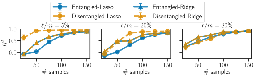
Figure 1: Test performance for the entangled and disentangled representation using Lasso and Ridge regression. All the results are averaged over $10$ seeds, with standard error shown in error bars.

We further assume that the task-specific matrices ${\bm{W}}^{(t)}$ are i.i.d. samples from some probability measure ${\mathbb{P}}_{\bm{W}}$ with support ${\mathcal{W}}$. We will see in Section 3.3 that the most critical assumptions of our theory concern ${\mathbb{P}}_{\bm{W}}$.

3.2 Main identifiability result

We are now ready to show the main theoretical result of this work, which provides a bi-level optimization problem for which the optimal representations are guaranteed to be disentangled. It assumes infinitely many tasks are observed, with task-specific ground-truth matrices ${\bm{W}}$ sampled from ${\mathbb{P}}_{\bm{W}}$. We denote by $\hat{\bm{W}}^{({\bm{W}})}$ the task-specific estimator of ${\bm{W}}$. We delay the presentation of its technical assumptions to Section 3.3. See Section B.2 for a proof.

Theorem 3.1 (Sparse multi-task learning for disentanglement).

Let $\hat{\bm{\theta}}$ be a minimizer of

$$\min_{\hat{\bm{\theta}}}\ {\mathbb{E}}_{{\mathbb{P}}_{\bm{W}}}{\mathbb{E}}_{p({\bm{x}},y\mid{\bm{W}})}-\log p(y;\hat{\bm{W}}^{({\bm{W}})}{\bm{f}}_{\hat{\bm{\theta}}}({\bm{x}}))$$ (2)

$$\mathrm{s.t.}\ \ \ \hat{\bm{W}}^{({\bm{W}})}\in\!\!\!\!\!\!\!\!\!\operatorname*{arg\,min}_{\begin{subarray}{c}\tilde{\bm{W}}\ \textnormal{s.t.}\\ ||\tilde{\bm{W}}||_{2,0}\leq||{\bm{W}}||_{2,0}\end{subarray}}\!\!\!\!\!\!\!\!\!{\mathbb{E}}_{p({\bm{x}},y\mid{\bm{W}})}-\log p(y;\tilde{\bm{W}}{\bm{f}}_{\hat{\bm{\theta}}}({\bm{x}}))\enspace,$$

where the constraint holds for all ${\bm{W}}\in{\mathcal{W}}$ and where ${\mathbb{P}}_{\bm{W}}$ and $p({\bm{x}},y\mid{\bm{W}})$ are described in Section 3.1. Under Assumptions 3.2, 3.3, 3.4, 3.5 and 3.6 and if ${\bm{f}}_{\tilde{\bm{\theta}}}$ is continuous for all $\tilde{\bm{\theta}}$, ${\bm{f}}_{\hat{\bm{\theta}}}$ is disentangled w.r.t. ${\bm{f}}_{\bm{\theta}}$ (Definition 1.1).

Intuitively, this optimization problem effectively selects a representation ${\bm{f}}_{\hat{\bm{\theta}}}$ that (i) allows a perfect fit of the data distribution, and (ii) allows the task-specific estimators $\hat{\bm{W}}^{({\bm{W}})}$ to be as sparse as the ground-truth ${\bm{W}}$. The theorem guarantees that such a representation must be disentangled.

Under the same assumptions and with the same disentanglement guarantees, Theorem B.6 in Appendix B presents a variation of Equation 2 which enforces the weaker constraint ${\mathbb{E}}_{{\mathbb{P}}_{\bm{W}}}\lVert\hat{\bm{W}}^{({\bm{W}})}\rVert_{2,0}\leq{\mathbb{E}}_{{\mathbb{P}}_{\bm{W}}}\lVert{\bm{W}}\rVert_{2,0}$, instead of $\lVert\hat{\bm{W}}^{({\bm{W}})}\rVert_{2,0}\leq\lVert{\bm{W}}\rVert_{2,0}$ for each task ${\bm{W}}$ individually.

Characteristic features of our theory. (i) Contrary to most identifiability results for disentanglement (Section 4), we do not assume the observations ${\bm{x}}$ are generated by transforming a latent random vector ${\bm{z}}$ through a bijective decoder ${\bm{g}}$. Instead, we assume the existence of a not necessarily invertible ground-truth feature extractor ${\bm{f}}_{\bm{\theta}}({\bm{x}})$ from which the labels can be predicted using only a subset of its components in every task. (ii) Most previous works make assumptions about the distribution of latent factors, e.g., (conditional) independence, exponential family or other parametric assumptions. In contrast, we make no such assumption except a rather weak assumption on the support of the ground-truth features (Assumption 3.3). Crucially, this allows for statistically dependent latent factors, which we explore empirically in Section 5.1.

3.3 Assumptions of Theorem 3.1

We now present the technical assumptions of Theorem 3.1.

Perhaps unsurprisingly, the parameters $\bm{\eta}$ have to be identifiable from $p(y;\bm{\eta})$ in order for ${\bm{f}}_{\bm{\theta}}$ to be identifiable.

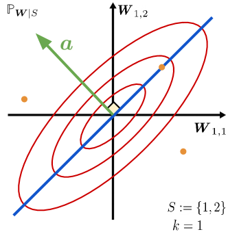
Figure 2: Illustration of Assumption 3.5 showing three examples of distribution ${\mathbb{P}}_{{\bm{W}}\mid S}$. The red distribution satisfies the assumption, but the blue and orange distributions do not. The red lines are level sets of a Gaussian distribution with full rank covariance. The blue line represents the support of a Gaussian distribution with a low-rank covariance. The orange dots represent a distribution with finite support. The green vector ${\bm{a}}$ shows that the condition is violated for both the blue and the orange distribution, since, in both cases, ${\bm{W}}_{1,S}$ and ${\bm{a}}$ are orthogonal (${\bm{W}}_{1,S}{\bm{a}}=0$) with probability greater than zero.

Assumption 3.2 (Identifiability of $\bm{\eta}$ from $p(y;\bm{\eta})$).

${\mathrm{KL}(p(y;\bm{\eta})\mid\mid p(y;\tilde{\bm{\eta}}))}=0\ \implies\bm{\eta}=\tilde{\bm{\eta}}$, where $\mathrm{KL}$ denotes the Kullback-Leibler divergence.

This property holds, e.g., when $p(y;\bm{\eta})$ is a Gaussian in the usual $\mu,\sigma^{2}$ parameterization. Generally, it also holds for minimal parameterizations of exponential families (Wainwright & Jordan, 2008).

The following assumption requires the ground-truth representation ${\bm{f}}_{\theta}({\bm{x}})$ to vary enough such that its image cannot be trapped inside a proper subspace.

Assumption 3.3 (Sufficient representation variability).

There exists ${\bm{x}}^{(1)},\dots,{\bm{x}}^{(m)}\in{\mathcal{X}}$ such that the matrix ${\bm{F}}:=[{\bm{f}}_{\bm{\theta}}({\bm{x}}^{(1)}),\dots,{\bm{f}}_{\bm{\theta}}({\bm{x}}^{(m)})]$ is invertible.

The following assumption requires that the support of the distribution ${\mathbb{P}}_{\bm{W}}$ is sufficiently rich.

Assumption 3.4 (Sufficient task variability).

There exists ${\bm{W}}^{(1)},\dots,{\bm{W}}^{(m)}\in{\mathcal{W}}$ and indices $i_{1},\dots,i_{m}\in[k]$ such that the rows ${\bm{W}}_{i_{1},:}^{(1)},\dots,{\bm{W}}_{i_{m},:}^{(m)}$ are linearly independent.

Under Assumptions 3.2, 3.3 and 3.4, the representation ${\bm{f}}_{\bm{\theta}}$ is identifiable up to linear equivalence (see Theorem B.4 in Appendix B). Similar results were shown by Roeder et al. (2021); Ahuja et al. (2022c). The next assumptions will guarantee disentanglement.

In order to formalize the intuitive idea that most tasks do not require all features, we will denote by $S^{(t)}$ the support of the matrix ${\bm{W}}^{(t)}$, i.e.,

$$S^{(t)}:=\{j\in[m]\mid{\bm{W}}^{(t)}_{:j}\not=\bm{0}\}\,.$$

In other words, $S^{(t)}$ is the set of features which are useful to predict $y$ in the $t$-th task; note that it is unknown to the learner. For our analysis, we decompose ${\mathbb{P}}_{\bm{W}}$ as

$${\mathbb{P}}_{\bm{W}}=\sum_{S\in{\mathcal{P}}([m])}p(S){\mathbb{P}}_{{\bm{W}}\mid S}\,,$$ (3)

where ${\mathcal{P}}([m])$ is the collection of all subsets of $[m]$, $p(S)$ is the probability that the support of ${\bm{W}}$ is $S$ and ${\mathbb{P}}_{{\bm{W}}\mid S}$ is the conditional distribution of ${\bm{W}}$ given that its support is $S$. Let ${\mathcal{S}}$ be the support of the distribution $p(S)$, i.e., ${\mathcal{S}}:=\{S\in{\mathcal{P}}([m])\mid p(S)>0\}$. The set ${\mathcal{S}}$ will have an important role in Assumption 3.6.

The following assumption requires that ${\mathbb{P}}_{{\bm{W}}\mid S}$ does not concentrate mass on certain proper subspaces.

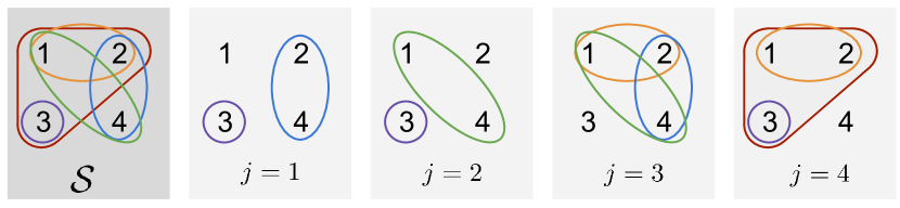
Figure 3: The leftmost figure represents ${\mathcal{S}}$, the set of task supports observed under the ground-truth distribution $p(S)$. The other figures form a verification that Assumption 3.6 holds for ${\mathcal{S}}$.

Assumption 3.5 (Intra-support sufficient task variability).

For all $S\in{\mathcal{S}}$ and all ${\bm{a}}\in{\mathbb{R}}^{|S|}\backslash\{0\}$,

$${\mathbb{P}}_{{\bm{W}}\mid S}\{{\bm{W}}\in{\mathbb{R}}^{k\times m}\mid{\bm{W}}_{:S}{\bm{a}}=\bm{0}\}=0\,.$$

We illustrate the above assumption in the simpler case where $k=1$. For instance, Assumption 3.5 holds when the distribution of ${\bm{W}}_{1,S}\mid S$ has a density w.r.t. the Lebesgue measure on ${\mathbb{R}}^{|S|}$, which is true for example when ${\bm{W}}_{1,S}\mid S\sim{\mathcal{N}}(\bm{0},\bm{\Sigma})$ and the covariance matrix $\bm{\Sigma}$ is full rank (red distribution in Fig. 2). However, if $\bm{\Sigma}$ is not full rank, the probability distribution of ${\bm{W}}_{1,S}\mid S$ concentrates its mass on a proper linear subspace $V\subsetneq{\mathbb{R}}^{|S|}$, which violates Assumption 3.5 (blue distribution in Fig. 2). Another important counter-example is when ${\mathbb{P}}_{{\bm{W}}\mid S}$ concentrates some of its mass on a point ${\bm{W}}^{(0)}$, i.e., ${\mathbb{P}}_{{\bm{W}}\mid S}\{{\bm{W}}^{(0)}\}>0$ (orange distribution in Fig. 2). We provide a concrete numerical example of what can go wrong when the support of the ${\mathbb{P}}_{{\bm{W}}\mid S}$ is finite in Section B.4. Interestingly, there are distributions over ${\bm{W}}_{1,S}\mid S$ that do not have a density w.r.t. the Lebesgue measure, but still satisfy Assumption 3.5. This is the case, e.g., when ${\bm{W}}_{1,S}\mid S$ puts uniform mass over a $(|S|-1)$-dimensional sphere embedded in ${\mathbb{R}}^{|S|}$ and centered at zero. See Section B.6 for a justification.

The following assumption requires that the support ${\mathcal{S}}$ of $p(S)$ is “rich enough”.

Assumption 3.6 (Sufficient variability of the task supports).

For all $j\in[m]$,

$$\bigcup_{S\in{\mathcal{S}}\mid j\not\in S}S=[m]\setminus\{j\}\,.$$

Intuitively, Assumption 3.6 requires that, for every feature $j$, one can find a set of tasks such that their supports cover all features except $j$ itself. Fig. 3 shows an example of ${\mathcal{S}}$ satisfying Assumption 3.6. Appendix B.5 provides a probabilistic argument showing that Assumption 3.6 holds “in most cases” when the number of supports is very large. That being said, we conjecture that removing this assumption would yield a form of partial disentanglement resembling the one developed by Lachapelle & Lacoste-Julien (2022) in which some groups of latent factors would remain entangled.

3.4 Tractable bilevel optimization problems for sparse multitask learning

The proposed approach to jointly estimate the representation and the task-specific predictors relies on a bilevel optimization problem (Equation 2) that is intractable because of the non-convex constraints. To obtain a tractable bi-level optimization problem, the $L_{2,0}$ constraints are replaced by their convex relaxations in the penalized form, which are also known to promote group sparsity (Argyriou et al., 2008):

$$\min_{\hat{\bm{\theta}}}\ \ -\frac{1}{Tn}\sum_{t=1}^{T}\sum_{({\bm{x}},y)\in{\mathcal{D}}_{t}}\log p(y;\hat{\bm{W}}^{(t)}{\bm{f}}_{\hat{\bm{\theta}}}({\bm{x}}))$$ (4)

$$\mathrm{s.t.}\ \,\hat{\bm{W}}^{(t)}\in\operatorname*{arg\,min}_{\tilde{\bm{W}}}\frac{1}{n}\sum_{({\bm{x}},y)\in{\mathcal{D}}_{t}}\!\!\!\!\!-\log p(y;\tilde{\bm{W}}{\bm{f}}_{\hat{\bm{\theta}}}({\bm{x}}))$$

$$\qquad\qquad\qquad\qquad\qquad\qquad\qquad\quad+\lambda_{t}||\tilde{\bm{W}}||_{2,1}\enspace,$$

where the constraint holds for all $t\in[T]$. Following Bengio (2000); Pedregosa (2016), one can compute the (hyper)gradient of the outer function using implicit differentiation, even if the inner optimization problem is non-smooth (Bertrand et al., 2020; Bolte et al., 2021; Malézieux et al., 2022; Bolte et al., 2022). Once the hypergradient is computed, one can optimize Equation 4 with usual first-order methods (Wright & Nocedal, 1999).

Note that the quantity $\hat{\bm{W}}^{(t)}{\bm{f}}_{\hat{\bm{\theta}}}({\bm{x}})$ is invariant to simultaneous rescaling of $\hat{\bm{W}}^{(t)}$ by a scalar and of ${\bm{f}}_{\hat{\bm{\theta}}}({\bm{x}})$ by its inverse. Thus, without constraints on ${\bm{f}}_{\hat{\bm{\theta}}}({\bm{x}})$, $\lVert\hat{\bm{W}}^{(t)}\rVert_{2,1}$ can be made arbitrarily small. This issue is similar to the one faced in sparse dictionary learning (Kreutz-Delgado et al., 2003; Mairal et al., 2008, 2009, 2011), where unit-norm constraints are usually imposed on dictionary columns. In our case, since ${\bm{f}}_{\hat{\bm{\theta}}}$ is parametrized by a neural network, we suggest applying batch or layer normalization (Ioffe & Szegedy, 2015; Ba et al., 2016) to control the norm of ${\bm{f}}_{\hat{\bm{\theta}}}({\bm{x}})$. Since the number of relevant features might be task-dependent,  Equation 4 has one regularization hyperparameter $\lambda_{t}$ per task. However, in practice, we select $\lambda_{t}:=\lambda$ for all $t\in[T]$ to limit the number of hyperparameters. We also use an adaptive scheme to have $\lambda$ in a reasonable range throughout training, which we explain in Section D.2.3.

Section B.3 introduces a similar relaxation of Theorem B.6 (mentioned in Section 3.2) in which the sparsity penalty appears in the outer problem instead of the inner problem. Section D.2.5 presents empirical results showing this alternative approach yields very similar results.

Link with meta-learning. The bi-level formulation Equation 4 is closely related to metric-based meta-learning methods (Snell et al., 2017; Bertinetto et al., 2019), where a shared representation ${\bm{f}}_{\hat{\bm{\theta}}}$ is learned across all tasks via simple task-specific predictors, such as linear classifiers. In the general meta-learning setting (Finn et al., 2017), one is given a large number of training datasets $({\mathcal{D}}_{t}^{\mathrm{train}})_{1\leq t\leq T}$, which usually only contain a small number of samples $n$. As opposed to the multi-task setting (i.e., unlike in Section 3.1), one is also given separate test datasets $({\mathcal{D}}_{t}^{\mathrm{test}})_{1\leq t\leq T}$ of $n^{\prime}$ samples for each task $t$, to evaluate how well the learned model generalizes to new test samples. In meta-learning, the goal is to learn a learning procedure that will generalize well on new unseen tasks.

Formally, metric-based meta-learning can be formulated as

$$\min_{\hat{\bm{\theta}}}\ \ \frac{1}{Tn^{\prime}}\sum_{t=1}^{T}\sum_{({\bm{x}},y)\in{\mathcal{D}}_{t}^{\mathrm{test}}}{\mathcal{L}}_{\mathrm{out}}\big{(}\hat{\bm{W}}_{\hat{\bm{\theta}}}^{(t)};f_{\hat{\bm{\theta}}}({\bm{x}}),y\big{)}$$ (5)

$$\mathrm{s.t.}\ \ \hat{\bm{W}}_{\hat{\bm{\theta}}}^{(t)}\in\operatorname*{arg\,min}_{\tilde{\bm{W}}}\frac{1}{n}\sum_{({\bm{x}},y)\in{\mathcal{D}}_{t}^{\mathrm{train}}}{\mathcal{L}}_{\mathrm{in}}\big{(}\tilde{\bm{W}};f_{\hat{\bm{\theta}}}({\bm{x}}),y\big{)}\enspace.$$

The main difference between Equation 4 and Equation 5 is that, in the latter, the inner and outer loss functions ${\mathcal{L}}_{\mathrm{in}}$ and ${\mathcal{L}}_{\mathrm{out}}$ are not evaluated on the same dataset. Section 5.2 shows experiments with a meta-learning variant of Equation 4 based on group Lasso multiclass SVM predictors.

4 Related Work

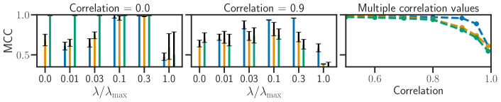
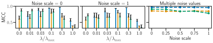
Figure 4: Disentanglement performance (MCC) for all three methods considered as a function of the regularization parameter (left and middle). Varying level of correlation between latents (top) and noise on the latents (bottom). The right columns show performances of the best hyperparameter for different values of correlation and noise. We explain what is $\lambda_{\max}$ in Section D.2.3.

Disentanglement. Since the work of Bengio et al. (2013), many methods have been proposed to learn disentangled representations based on various heuristics (Higgins et al., 2017; Chen et al., 2018; Kim & Mnih, 2018; Kumar et al., 2018; Bouchacourt et al., 2018). Following the work of Locatello et al. (2019), which highlighted the lack of identifiability in modern deep generative models, many works have proposed more or less weak forms of supervision motivated by identifiability analyses (Locatello et al., 2020a; Klindt et al., 2021; Von Kügelgen et al., 2021; Ahuja et al., 2022a, c; Zheng et al., 2022). A similar line of work have adopted the causal representation learning perspective (Lachapelle et al., 2022; Lachapelle & Lacoste-Julien, 2022; Lippe et al., 2022b, a; Ahuja et al., 2022b; Yao et al., 2022; Brehmer et al., 2022).

The problem of identifiability was well known among the independent component analysis (ICA) community (Hyvärinen et al., 2001; Hyvärinen & Pajunen, 1999) which came up with solutions for general nonlinear mixing functions by leveraging auxiliary information (Hyvärinen & Morioka, 2016, 2017; Hyvärinen et al., 2019; Khemakhem et al., 2020a, b). Another approach is to consider restricted hypothesis classes of mixing functions (Taleb & Jutten, 1999; Gresele et al., 2021; Zheng et al., 2022; Moran et al., 2022). Locatello et al. (2020b) proposed a semi-supervised learning approach to disentangle in cases where a few samples are labelled with the values of the factors of variations themselves. This is different from our approach as the labels that we consider can be sampled from some $p(y;{\bm{W}}{\bm{f}}_{\hat{\bm{\theta}}}({\bm{x}}))$, which is more general. Ahuja et al. (2022c) consider a setting similar to ours, but they rely on the independence and non-gaussianity of the latent factors for disentanglement using linear ICA. See the end of Section 3.2 for further discussions on how our theory distinguishes itself from most methods cited above.

Multi-task, transfer & invariant learning. While the statistical advantages of multi-task representation learning are well understood (Lounici et al., 2011a, b; Maurer et al., 2016), the theoretical benefits of disentanglement for transfer learning are not clearly established (apart from Zhang et al. 2022). Some works have investigated this question empirically and obtained both positive (van Steenkiste et al., 2019; Miladinović et al., 2019; Dittadi et al., 2021) and negative results (Locatello et al., 2019; Montero et al., 2021). Invariant risk minimization (Arjovsky et al., 2020; Ahuja et al., 2020; Krueger et al., 2021; Lu et al., 2021) aims at learning a representation that elicits a single predictor that is optimal for all tasks. This differs from our approach which learns one predictor per task.

Dictionary learning and sparse coding. We contrast our approach, which jointly learns a dense representation and sparse task-specific predictors (Equation 4), with the line of work which consists in learning sparse representations (Chen et al., 1998; Gribonval & Lesage, 2006). For instance, sparse dictionary learning (Mairal et al., 2009, 2011; Maurer et al., 2013) is an unsupervised technique that aims at learning a dictionary of atoms used to reconstruct inputs via sparse linear combinations of its elements. The representation of a single input consists of the coefficients of the linear combination of atoms that minimizes a sparsity-regularized reconstruction loss. In the case of supervised dictionary learning (Mairal et al., 2008), an additional (potentially expressive) classifier is learned on top of that representation. This large literature has led to a wide variety of estimators: for instance, Mairal et al. (2008, Eq. 4), which minimizes the sum of the classification error and the approximation error of the code, or Mairal et al. (2011). introducing bi-level formulations. While sharing similar optimization challenges, our method is conceptually different and computes the representation of a single input ${\bm{x}}$ by evaluating the learned function ${\bm{f}}_{\hat{\bm{\theta}}}$.

5 Experiments

We present experiments on disentanglement and few-shot learning. Our implementation relies on jax and jaxopt (Bradbury et al., 2018; Blondel et al., 2022) and is available here: https://github.com/tristandeleu/synergies-disentanglement-sparsity.

5.1 Disentanglement in 3D Shapes

We now illustrate Theorem 3.1 by applying Equation 4 to tasks generated using the 3D Shapes dataset (Burgess & Kim, 2018).

Data generation. For all tasks $t$, the labelled dataset ${\mathcal{D}}_{t}=\{({\bm{x}}^{(t,i)}),y^{(t,i)})\}_{i=1}^{n}$ is generated by first sampling the ground-truth latent variables ${\bm{z}}^{(t,i)}$ i.i.d. according to some distribution $p({\bm{z}})$, while the corresponding input is obtained doing ${\bm{x}}^{(t,i)}:={\bm{f}}_{\bm{\theta}}^{-1}({\bm{z}}^{(t,i)})$ (${\bm{f}}_{\bm{\theta}}$ is invertible in 3D Shapes). Then, a sparse weight vector ${\bm{w}}^{(t)}$ is sampled randomly to compute the labels of each example as $y^{(t,i)}:={\bm{w}}^{(t)}\cdot{\bm{z}}^{(t,i)}+\epsilon^{(t,i)}$, where $\epsilon^{(t,i)}$ is independent Gaussian noise. Fig. 4 explores various choices of $p({\bm{z}})$ by varying the level of correlation between the latent variables and by varying the level of noise on the ground-truth latents. See Section D.2 for more details about the data generating process and Fig. 7 to visualize various $p({\bm{z}})$.

Algorithms. In this setting where $p(y;\bm{\eta})$ is a Gaussian with fixed variance, the inner problem of Equation 4 amounts to Lasso regression, we thus refer to this approach as inner-Lasso. We also evaluate a simple variation of Equation 4 in which the $L_{1}$ norm is replaced by an $L_{2}$ norm and refer to it as inner-Ridge. In addition, we evaluate the representation obtained by performing linear ICA (Comon, 1992) on the representation learned by inner-Ridge: the case $\lambda=0$ corresponds to the approach of Ahuja et al. (2022c).

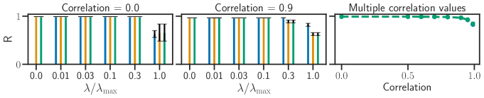
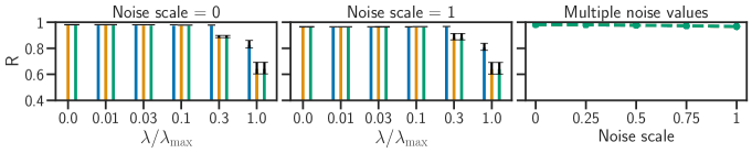
Figure 6: Prediction performance (R Score) for inner-Lasso, inner-Ridge and inner-Ridge combined with ICA as a function of the regularization parameter (left and middle). Varying level of correlation between latents (top) and noise on the latents (bottom). The right columns shows performance of the best hyperparameter for different values of correlation and noise levels.

Discussion. Fig. 4 reports disentanglement performances of the three methods, as measured by the mean correlation coefficient, or MCC (Hyvärinen & Morioka, 2016; Khemakhem et al., 2020a) (Section D.2). In all settings, inner-Lasso obtains high MCC for some values of $\lambda$, being on par or surpassing the baselines. As the theory suggests, it is robust to high levels of correlations between the latents, as opposed to inner-Ridge with ICA which is very much affected by strong correlations (since ICA assumes independence). We can also see how additional noise on the latent variables hurts inner-Ridge with ICA while leaving inner-Lasso unaffected. Fig. 6 in Section D.2 shows that all methods find a representation which is linearly equivalent to the ground-truth representation, except for very large values of $\lambda$. Section D.2.4 studies empirically to what extent inner-Lasso is robust to violations of Assumption 3.6, Section D.2.6 presents a visual evaluation of disentanglement and Section D.2.7 reports the DCI metric (Eastwood & Williams, 2018) on the same experiments. We did not explore hyperparameter selection in this work, which is a difficult problem for disentanglement because a goodness-of-fit score evaluated on a held-out dataset will not be informative because of the lack of identifiability. Nevertheless, one can use heuristics such as the unsupervised disentanglement ranking score proposed by Duan et al. (2020).

5.2 Sparse task-specific predictors in few-shot learning

Despite the lack of ground-truth latent factors in standard few-shot learning benchmarks, we also evaluate sparse meta-learning objectives on the miniImageNet dataset (Vinyals et al., 2016). The purpose of this experiment is to show that the sparse formulation of standard metric-based meta-learning techniques reaches similar performance while using a fraction of the features (Fig. 5, right).

Inspired by Lee et al. (2019), where the task-specific classifiers are multiclass support-vector machines (SVMs, Crammer & Singer 2001), we propose to use group Lasso penalized multiclass SVMs, to introduce sparsity in the classifiers. Using the notation of Equation 5, we choose

$${\mathcal{L}}_{\mathrm{in}}({\bm{W}};f_{\hat{\bm{\theta}}}({\bm{x}}_{i}),{\bm{y}}_{i}) =\max_{l\in[k]}\left(({\bm{W}}_{{\bm{y}}_{i}:}-{\bm{W}}_{l:})\cdot f_{\hat{\bm{\theta}}}({\bm{x}}_{i})-{\bm{Y}}_{il}\right)$$

$$+\lambda_{1}\lVert{\bm{W}}\rVert_{2,1}+\tfrac{\lambda_{2}}{2}\lVert{\bm{W}}\rVert^{2}\enspace,$$ (6)

$${\mathcal{L}}_{\mathrm{out}}({\bm{W}};f_{\hat{\bm{\theta}}}({\bm{x}}_{i}),{\bm{y}}_{i}) =\mathrm{CE}({\bm{W}}f_{\hat{\bm{\theta}}}({\bm{x}}_{i}),{\bm{Y}}_{i:})\enspace,$$ (7)

with ${\bm{Y}}\in\mathbb{R}^{n\times k}$ the one-hot encoding of ${\bm{y}}\in{\mathbb{R}}^{n}$ and $\mathrm{CE}$ the cross-entropy. The difference with Lee et al. (2019) is the sparsity-promoting term $\lVert{\bm{W}}\rVert_{2,1}$, which makes the bi-level optimization problem harder to solve. That is why we propose solving the dual (Boyd et al., 2004, Chap. 5) of this inner optimization problem, which writes

$$\min_{{\bm{\Lambda}}\in{\mathbb{R}}^{n\times k}}\frac{1}{\lambda_{2}}\sum_{j=1}^{m}\lVert\mathrm{BST}\left(({\bm{Y}}-{\bm{\Lambda}})^{\top}{\bm{F}}_{:j},\lambda_{1}\right)\rVert^{2}+\langle{\bm{Y}},{\bm{\Lambda}}\rangle$$

$$\mathrm{s.t.}\;\forall i,l,\in[n]\times[k],\;\sum\limits_{l^{\prime}=1}^{k}{\bm{\Lambda}}_{il^{\prime}}=1\;\text{ and }\;{\bm{\Lambda}}_{il}\geq 0\enspace,$$ (8)

with $\mathrm{BST}:({\bm{a}},\tau)\mapsto\left(1-{\tau}/{\left\lVert{\bm{a}}\right\rVert}\right)_{+}{\bm{a}}$ is the block soft-thresholding operator, ${\bm{F}}\in{\mathbb{R}}^{n\times m}$ the concatenation of $\{{\bm{f}}_{\hat{\bm{\theta}}}(x)\}_{(x,y)\in{\mathcal{D}}^{\mathrm{train}}}$.  In addition, the primal-dual link writes, $\forall j\in[m],\ {\bm{W}}_{:j}=\mathrm{BST}\left(({\bm{Y}}-{\bm{\Lambda}})^{\top}{\bm{F}}_{:j},\lambda_{1}\right)/\lambda_{2}$. The derivation of the dual can be found in Section C.1, Solving this kind of problem in the dual is standard in the SVM literature: it has been proven to be computationally advantageous (Hsieh et al., 2008) when the number of features $m$ is significantly larger than the number of samples $n$ (here $m=1.6\times 10^{4}$ and $n\leq 25$). Details on how to solve and differentiate through Equation 8 are in Section D.3.

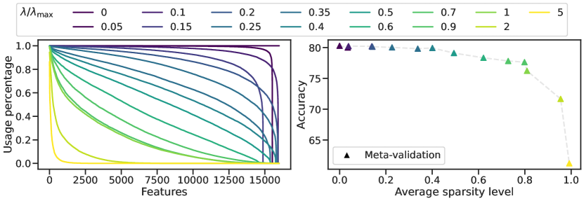
Figure 5: Left. Effect of sparsity on the percentage of tasks using specific features, with our meta-learning objective, on miniImageNet. Right. The meta-validation accuracy of the meta-learning algorithm against the average level of sparsity in the task-specific predictor, for different values of $\lambda$.

Discussion. In Fig. 5 (right), we observe that the accuracy of the sparse meta-learning method on novel (meta-validation) tasks is similar to the dense counterpart ($\lambda=0$), while using only a few of the features available (around $30\%$ of sparsity, with no impact on the performance). Naturally, the performance starts to drop as the sparsity level increases though, albeit being still competitive. We also report in Fig. 5 (left) how frequently each feature in the learned representation is used by the task-specific predictors on meta-validation tasks (sorted by usage, for each $\lambda$). The gradual decrease in usage suggests that the features are reused in different contexts, across different tasks.

6 Conclusion

In this work, we investigated the synergies between sparsity, disentanglement and generalization. We showed that when the downstream task can be solved using only a fraction of the factors of variations, disentangled representations combined with sparse task-specific predictors can improve generalization (Section 2). Our novel identifiability result (Theorem 3.1) sheds light on how, in a multi-task setting, sparsity regularization on the task-specific predictors can induce disentanglement. This led to a practical bi-level optimization problem that was shown to yield disentangled representations on regression tasks based on the 3D Shapes dataset. Finally, we explored the connection between this bi-level formulation and meta-learning, and we showed how sparse task-specific predictors may achieve similar performance on unseen tasks with only a fraction of the features. Future work could explore identifiability in a more general setting where the task-specific predictors are potentially nonlinear, which should be applicable to more problems.

Part Appendix

Table 1: Table of Notations.

Norms & pseudonorms
$\left\lVert\cdot\right\rVert$		Euclidean norm on vectors and Frobenius norm on matrices
$\left\lVert{\bm{A}}\right\rVert_{2,1}$	$:=$	$\sum_{j=1}^{m}\left\lVert{\bm{A}}_{:j}\right\rVert$
$\left\lVert{\bm{A}}\right\rVert_{2,0}$	$:=$	$\sum_{j=1}^{m}\mathbbm{1}_{\left\lVert{\bm{A}}_{:j}\right\rVert\neq 0}$, where $\mathbbm{1}$ is the indicator function.
Data
${\bm{x}}\in{\mathbb{R}}^{d}$		Observations
${\mathcal{X}}\subset{\mathbb{R}}^{d}$		Support of observations
$y\in{\mathbb{R}}$		Target
${\mathcal{Y}}\subset{\mathbb{R}}$		Support of targets
Learned/ground-truth model
${\bm{W}}\in{\mathbb{R}}^{k\times m}$		Ground-truth coefficients
$\hat{\bm{W}}\in{\mathbb{R}}^{k\times m}$		Learned coefficients
${\bm{\theta}}$		Ground-truth parameters of the representation
$\hat{\bm{\theta}}$		Learned parameters of the representation
$f_{{\bm{\theta}}}:{\mathbb{R}}^{d}\rightarrow{\mathbb{R}}^{m}$		Ground-truth representation
$f_{\hat{\bm{\theta}}}:{\mathbb{R}}^{d}\rightarrow{\mathbb{R}}^{m}$		Learned representation
$\bm{\eta}\in{\mathbb{R}}^{k}$		Parameter of the distribution $p(y;\bm{\eta})$
${\mathbb{P}}_{\bm{W}}$		Distribution over ground-truth coefficient matrices ${\bm{W}}$
$S$	$:=$	$\{j\in[m]\mid{\bm{W}}_{:j}\not=\bm{0}\}$ (support of ${\bm{W}}$)
${\mathbb{P}}_{{\bm{W}}\mid S}$		Conditional distribution of ${\bm{W}}$ given $S$.
$p(S)$		Ground-truth distribution over possible supports $S$
${\mathcal{S}}$		Support of the distribution $p(S)$
Optimization
$W$		Primal variable
$\Lambda$		Dual variable
$h^{*}:{\bm{a}}$	$\mapsto$	$\sup_{{\bm{b}}\in{\mathbb{R}}^{d}}\langle{\bm{a}},{\bm{b}}\rangle-h({\bm{b}})$, Fenchel conjugate of the function $h:{\mathbb{R}}^{d}\rightarrow{\mathbb{R}}$
$f\square g:{\bm{a}}$	$\mapsto$	$\min_{b}f({\bm{a}}-{\bm{b}})+g({\bm{b}})$ , inf-convolution of the functions $f$ and $g$
$\mathrm{BST}:({\bm{a}},\tau)$	$\mapsto$	$\left(1-{\tau}/{\left\lVert{\bm{a}}\right\rVert}\right)_{+}{\bm{a}}$, block soft-thresholding operator

Appendix A Proofs of Section 2

See 2.2

Proof.

By definition of $\hat{\bm{W}}^{(\hat{\bm{\theta}})}$, we have that, for all $\hat{\bm{W}}\in{\mathbb{R}}^{k\times m}$,

$$\sum_{({\bm{x}},y)\in{\mathcal{D}}}\log p(y;\hat{\bm{W}}^{(\hat{\bm{\theta}})}{\bm{f}}_{\hat{\bm{\theta}}}({\bm{x}})) \geq\sum_{({\bm{x}},y)\in{\mathcal{D}}}\log p(y;\hat{\bm{W}}{\bm{f}}_{\hat{\bm{\theta}}}({\bm{x}}))$$ (9)

$$\sum_{({\bm{x}},y)\in{\mathcal{D}}}\log p(y;\hat{\bm{W}}^{(\hat{\bm{\theta}})}{\bm{L}}{\bm{f}}_{{\bm{\theta}}}({\bm{x}})) \geq\sum_{({\bm{x}},y)\in{\mathcal{D}}}\log p(y;\hat{\bm{W}}{\bm{L}}{\bm{f}}_{{\bm{\theta}}}({\bm{x}}))\,.$$ (10)

Because ${\mathbb{R}}^{k\times m}{\bm{L}}={\mathbb{R}}^{k\times m}$, we have that, for all $\hat{\bm{W}}\in{\mathbb{R}}^{k\times m}$,

$$\sum_{({\bm{x}},y)\in{\mathcal{D}}}\log p(y;\hat{\bm{W}}^{(\hat{\bm{\theta}})}{\bm{L}}{\bm{f}}_{{\bm{\theta}}}({\bm{x}})) \geq\sum_{({\bm{x}},y)\in{\mathcal{D}}}\log p(y;\hat{\bm{W}}{\bm{f}}_{{\bm{\theta}}}({\bm{x}}))\,,$$ (11)

which is to say that $\hat{\bm{W}}^{({\bm{\theta}})}=\hat{\bm{W}}^{(\hat{\bm{\theta}})}{\bm{L}}$, or put differently, $\hat{\bm{W}}^{(\hat{\bm{\theta}})}=\hat{\bm{W}}^{({\bm{\theta}})}{\bm{L}}^{-1}$. It implies

$$\hat{\bm{W}}^{(\hat{\bm{\theta}})}{\bm{f}}_{\hat{\bm{\theta}}}({\bm{x}})=\hat{\bm{W}}^{({\bm{\theta}})}{\bm{L}}^{-1}{\bm{L}}{\bm{f}}_{{\bm{\theta}}}({\bm{x}})=\hat{\bm{W}}^{({\bm{\theta}})}{\bm{f}}_{{\bm{\theta}}}({\bm{x}})\,,$$ (12)

which is what we wanted to show. ∎

See 2.4

Proof.

By definition of $\hat{\bm{W}}_{\infty}^{(\hat{\bm{\theta}})}$, we have that, for all $\tilde{\bm{W}}\in{\mathbb{R}}^{k\times m}$,

$${\mathbb{E}}_{p({\bm{x}},y)}\log p(y;\hat{\bm{W}}_{\infty}^{(\hat{\bm{\theta}})}{\bm{f}}_{\hat{\bm{\theta}}}({\bm{x}})) \geq{\mathbb{E}}_{p({\bm{x}},y)}\log p(y;\tilde{\bm{W}}{\bm{f}}_{\hat{\bm{\theta}}}({\bm{x}}))$$ (13)

$${\mathbb{E}}_{p({\bm{x}},y)}\log p(y;\hat{\bm{W}}_{\infty}^{(\hat{\bm{\theta}})}{\bm{L}}{\bm{f}}_{{\bm{\theta}}}({\bm{x}})) \geq{\mathbb{E}}_{p({\bm{x}},y)}\log p(y;\tilde{\bm{W}}{\bm{L}}{\bm{f}}_{{\bm{\theta}}}({\bm{x}}))\,.$$ (14)

In particular, the inequality holds for $\tilde{\bm{W}}:={\bm{W}}{\bm{L}}^{-1}$, which yields

$${\mathbb{E}}_{p({\bm{x}},y)}\log p(y;\hat{\bm{W}}_{\infty}^{(\hat{\bm{\theta}})}{\bm{L}}{\bm{f}}_{{\bm{\theta}}}({\bm{x}})) \geq{\mathbb{E}}_{p({\bm{x}},y)}\log p(y;{\bm{W}}{\bm{f}}_{{\bm{\theta}}}({\bm{x}}))$$ (15)

$$0 \geq{\mathbb{E}}_{p({\bm{x}},y)}\left[\log p(y;{\bm{W}}{\bm{f}}_{{\bm{\theta}}}({\bm{x}}))-\log p(y;\hat{\bm{W}}_{\infty}^{(\hat{\bm{\theta}})}{\bm{L}}{\bm{f}}_{{\bm{\theta}}}({\bm{x}}))\right]$$ (16)

$$0 \geq{\mathbb{E}}_{p({\bm{x}})}\text{KL}(p(y;{\bm{W}}{\bm{f}}_{{\bm{\theta}}}({\bm{x}}))\mid\mid p(y;\hat{\bm{W}}_{\infty}^{(\hat{\bm{\theta}})}{\bm{L}}{\bm{f}}_{{\bm{\theta}}}({\bm{x}})))\,.$$ (17)

Since the KL is always non-negative, we have that,

$${\mathbb{E}}_{p({\bm{x}})}\text{KL}(p(y;{\bm{W}}{\bm{f}}_{{\bm{\theta}}}({\bm{x}}))\mid\mid p(y;\hat{\bm{W}}_{\infty}^{(\hat{\bm{\theta}})}{\bm{L}}{\bm{f}}_{{\bm{\theta}}}({\bm{x}})))=0\,,$$ (18)

which in turn implies

$${\mathbb{E}}_{p({\bm{x}},y)}\log p(y;\hat{\bm{W}}_{\infty}^{(\hat{\bm{\theta}})}{\bm{L}}{\bm{f}}_{{\bm{\theta}}}({\bm{x}})) ={\mathbb{E}}_{p({\bm{x}},y)}\log p(y;{\bm{W}}{\bm{f}}_{{\bm{\theta}}}({\bm{x}}))$$ (19)

$${\mathbb{E}}_{p({\bm{x}},y)}\log p(y;\hat{\bm{W}}_{\infty}^{(\hat{\bm{\theta}})}{\bm{L}}{\bm{f}}_{{\bm{\theta}}}({\bm{x}})) ={\mathbb{E}}_{p({\bm{x}},y)}\log p(y;{\bm{W}}{\bm{L}}^{-1}{\bm{L}}{\bm{f}}_{{\bm{\theta}}}({\bm{x}}))$$ (20)

$${\mathbb{E}}_{p({\bm{x}},y)}\log p(y;\hat{\bm{W}}_{\infty}^{(\hat{\bm{\theta}})}{\bm{f}}_{\hat{\bm{\theta}}}({\bm{x}})) ={\mathbb{E}}_{p({\bm{x}},y)}\log p(y;{\bm{W}}{\bm{L}}^{-1}{\bm{f}}_{\hat{\bm{\theta}}}({\bm{x}}))$$ (21)

Since the solution to the population MLE from Proposition 2.4 is assumed to be unique, this equality holds if and only if $\hat{\bm{W}}_{\infty}^{(\hat{\bm{\theta}})}={\bm{W}}{\bm{L}}^{-1}$. ∎

Appendix B Proofs of Section 3

B.1 Technical Lemmas

The lemmas of this section can be skipped at first read.

The following lemma will be important for proving Theorem B.5. The argument is taken from Lachapelle et al. (2022).

Lemma B.1 (Sparsity pattern of an invertible matrix contains a permutation).

Let ${\bm{L}}\in{\mathbb{R}}^{m\times m}$ be an invertible matrix. Then, there exists a permutation $\sigma$ such that ${\bm{L}}_{i,\sigma(i)}\not=0$ for all $i$.

Proof.

Since the matrix ${\bm{L}}$ is invertible, its determinant is non-zero, i.e.,

$$\det({\bm{L}}):=\sum_{\sigma\in\mathfrak{S}_{m}}\text{sign}(\sigma)\prod_{i=1}^{m}{\bm{L}}_{i,\sigma(i)}\neq 0\,,$$ (23)

where $\mathfrak{S}_{m}$ is the set of $m$-permutations. This equation implies that at least one term of the sum is non-zero, meaning there exists $\sigma\in\mathfrak{S}_{m}$ such that for all $i\in[m]$, ${\bm{L}}_{i,\sigma(i)}\neq 0$. ∎

The following technical lemma will help us dealing with almost-everywhere statements and can be safely skipped at a first read. Before presenting it, we recall the formal definition of a support of a distribution.

Definition B.2.

The support of a Borel measure $\mu$ over a topological space $(X,\tau)$ is the set of point $x\in X$ such that, for all open set $U\in\tau$ containing $x$, $\mu(U)>0$.

Throughout this work, we assume implicitly that all measures are Borel measures with respect to the standard topology of the space on which they are defined.

Lemma B.3.

Assumption 3.4 is equivalent to the following statement: For all $E_{0}\subset{\mathbb{R}}^{k\times m}$ such that ${\mathbb{P}}_{\bm{W}}(E_{0})=0$, there exists ${\bm{W}}^{(1)},\dots,{\bm{W}}^{(m)}\in{\mathcal{W}}\setminus E_{0}$ and indices $i_{1},...,i_{m}\in[k]$ such that the row vectors ${\bm{W}}^{(1)}_{i_{1},:},\dots,{\bm{W}}^{(m)}_{i_{m},:}$ are linearly independent.

Proof.

First of all, the "$\impliedby$" direction is trivial since one can simply pick $E_{0}=\emptyset$.

We now show the "$\implies$" direction. First of all, we notice that, since ${\bm{W}}^{(1)}_{i_{1},:},\dots,{\bm{W}}^{(m)}_{i_{m},:}$ are linearly independent, they form a matrix with nonzero determinant, i.e.,

$$\det\begin{bmatrix}{\bm{W}}^{(1)}_{i_{1},:}\\ \vdots\\ {\bm{W}}^{(m)}_{i_{m},:}\end{bmatrix}\not=0\,.$$ (24)

Define the map $\eta:({\mathbb{R}}^{k\times m})^{m}\rightarrow{\mathbb{R}}^{m\times m}$ as

$$\eta(\bar{\bm{W}}^{(1)},\dots,\bar{\bm{W}}^{(m)}):=\begin{bmatrix}\bar{\bm{W}}^{(1)}_{i_{1},:}\\ \vdots\\ \bar{\bm{W}}^{(m)}_{i_{m},:}\end{bmatrix},\ \forall(\bar{\bm{W}}^{(1)},\dots,\bar{\bm{W}}^{(m)})\in({\mathbb{R}}^{k\times m})^{m}\,,$$ (25)

which is continuous. Note that $\det(\cdot)$ is also a continuous map, hence $\det\circ\eta$ is continuous as well. Thus, the set $V:=(\det\circ\eta)^{-1}({\mathbb{R}}\setminus\{0\})$ is open (since ${\mathbb{R}}\setminus\{0\}$ is open). Let ${\mathbb{P}}_{{\bm{W}}}^{m}$ be the product measure over tuples of matrices $(\bar{\bm{W}}^{(1)},\dots,\bar{\bm{W}}^{(m)})$. Note that its support is ${\mathcal{W}}^{m}$. Because $({\bm{W}}^{(1)},...,{\bm{W}}^{(m)})$ is in the open set $V$ and in the support of ${\mathbb{P}}_{\bm{W}}^{m}$, we have that

$$0 <{\mathbb{P}}_{{\bm{W}}}^{m}(V)$$ (26)

$$={\mathbb{P}}_{{\bm{W}}}^{m}(V\cap{\mathcal{W}}^{m})+{\mathbb{P}}_{{\bm{W}}}^{m}(V\cap({\mathcal{W}}^{m})^{c})$$ (27)

$$\leq{\mathbb{P}}_{{\bm{W}}}^{m}(V\cap{\mathcal{W}}^{m})+{\mathbb{P}}_{{\bm{W}}}^{m}(({\mathcal{W}}^{m})^{c})$$ (28)

$$={\mathbb{P}}_{{\bm{W}}}^{m}(V\cap{\mathcal{W}}^{m})$$ (29)

Let $E_{0}\subset{\mathbb{R}}^{k\times m}$ be such that ${\mathbb{P}}_{\bm{W}}(E_{0})=0$. Then, we also have that ${\mathbb{P}}_{\bm{W}}^{m}(E_{0}^{m})=0$ and thus

$${\mathbb{P}}_{{\bm{W}}}^{m}((V\cap{\mathcal{W}}^{m})\setminus E_{0}^{m})>0\,.$$ (30)

This implies that the set $((\det\circ\eta)^{-1}({\mathbb{R}}\setminus\{0\})\cap{\mathcal{W}}^{m})\setminus E_{0}^{m}$ is not empty, i.e., there exists $(\bar{\bm{W}}^{(1)},\dots,\bar{\bm{W}}^{(m)})\in{\mathcal{W}}^{m}\setminus E_{0}^{m}$ such that the rows $\bar{\bm{W}}^{(1)}_{i_{1},:},\dots,\bar{\bm{W}}^{(m)}_{i_{m},:}$ are linearly independent. Since the measure zero set $E_{0}$ was arbitrary, this concludes the proof. ∎

B.2 Proof of Theorem 3.1

This section presents the main results building up to Theorem 3.1.

For all ${\bm{W}}\in{\mathcal{W}}$, we are going to denote by $\hat{\bm{W}}^{({\bm{W}})}$ some estimator of ${\bm{W}}$. The following result provides conditions under which if $\hat{\bm{W}}^{({\bm{W}})}$ allows a perfect fit of the ground-truth distribution $p(y\mid{\bm{x}},{\bm{W}})$, then the representation ${\bm{f}}_{\bm{\theta}}$ and the parameter ${\bm{W}}$ are identified up to an invertible linear transformation. Many works have showed similar results in various context (Hyvärinen & Morioka, 2016; Khemakhem et al., 2020a; Roeder et al., 2021; Ahuja et al., 2022c). We reuse some of their proof techniques.

Theorem B.4 (Linear identifiability).

Let $\hat{\bm{W}}^{(\cdot)}:{\mathcal{W}}\rightarrow{\mathbb{R}}^{k\times m}$. Suppose Assumptions 3.2, 3.3 and 3.4 hold and that, for ${\mathbb{P}}_{\bm{W}}$-almost every ${\bm{W}}\in{\mathcal{W}}$ and all ${\bm{x}}\in{\mathcal{X}}$, the following holds

$$\mathrm{KL}(p(y;\hat{\bm{W}}^{({\bm{W}})}{\bm{f}}_{\hat{\bm{\theta}}}({\bm{x}}))||p(y;{\bm{W}}{\bm{f}}_{{\bm{\theta}}}({\bm{x}}))=0\enspace.$$ (31)

Then, there exists an invertible matrix ${\bm{L}}\in{\mathbb{R}}^{m\times m}$ such that, for all ${\bm{x}}\in{\mathcal{X}}$, ${\bm{f}}_{\bm{\theta}}({\bm{x}})={\bm{L}}{{\bm{f}}}_{\hat{\bm{\theta}}}({\bm{x}})$ and such that, for ${\mathbb{P}}_{\bm{W}}$-almost every ${\bm{W}}\in{\mathcal{W}}$, $\hat{\bm{W}}^{({\bm{W}})}={\bm{W}}{\bm{L}}$

Proof.

By Assumption 3.2, Equation 31 implies that, for ${\mathbb{P}}_{\bm{W}}$-almost every ${\bm{W}}$ and all ${\bm{x}}\in{\mathcal{X}}$, ${\bm{W}}{\bm{f}}_{\bm{\theta}}({\bm{x}})=\hat{\bm{W}}^{({\bm{W}})}{\bm{f}}_{\hat{\bm{\theta}}}({\bm{x}})$. Assumption 3.4 combined with Lemma B.3 ensures that we can construct an invertible matrix ${\bm{U}}:=\begin{bmatrix}{\bm{W}}_{i_{1},:}^{(1)}\\ \vdots\\ {\bm{W}}_{i_{d_{z}},:}^{(d_{z})}\end{bmatrix}$ such that ${\bm{U}}{\bm{f}}_{\bm{\theta}}({\bm{x}})=\hat{\bm{U}}{\bm{f}}_{\hat{\bm{\theta}}}({\bm{x}})$ for all ${\bm{x}}\in{\mathcal{X}}$ where $\hat{\bm{U}}:=\begin{bmatrix}\hat{\bm{W}}_{i_{1},:}^{({\bm{W}}^{(1)})}\\ \vdots\\ \hat{\bm{W}}_{i_{d_{z}},:}^{({\bm{W}}^{(d_{z})})}\end{bmatrix}$. Left-multiplying by ${\bm{U}}^{-1}$ on both sides yields ${\bm{f}}_{\bm{\theta}}({\bm{x}})={\bm{L}}{\bm{f}}_{\hat{\bm{\theta}}}({\bm{x}})$, where ${\bm{L}}:={\bm{U}}^{-1}\hat{\bm{U}}$. Using the invertible matrix ${\bm{F}}$ from Assumption 3.3, we can thus write ${\bm{F}}={\bm{L}}\hat{\bm{F}}$ where we defined $\hat{\bm{F}}:=[{\bm{f}}_{\hat{\bm{\theta}}}({\bm{x}}^{(1)}),\cdots,{\bm{f}}_{\hat{\bm{\theta}}}({\bm{x}}^{(d_{z})})]$. Since ${\bm{F}}$ is invertible, so are ${\bm{L}}$ and $\hat{\bm{F}}$.

By substituting ${\bm{F}}={\bm{L}}\hat{\bm{F}}$ in ${\bm{W}}{\bm{F}}=\hat{\bm{W}}^{({\bm{W}})}\hat{\bm{F}}$, we obtain ${\bm{W}}{\bm{L}}\hat{\bm{F}}=\hat{\bm{W}}^{({\bm{W}})}\hat{\bm{F}}$. By right-multiplying both sides by $\hat{\bm{F}}^{-1}$, we obtain ${\bm{W}}{\bm{L}}=\hat{\bm{W}}^{({\bm{W}})}$. ∎

The following theorem is where most of the theoretical contribution of this work lies. Note that Theorem 3.1, from the main text, is a straightforward application of this result.

Theorem B.5.

(Disentanglement via task sparsity) Let $\hat{\bm{W}}^{(\cdot)}:{\mathcal{W}}\rightarrow{\mathbb{R}}^{k\times m}$. Suppose Assumptions 3.2, 3.3, 3.4, 3.5 and 3.6 hold and that, for ${\mathbb{P}}_{\bm{W}}$-almost every ${\bm{W}}\in{\mathcal{W}}$ and all ${\bm{x}}\in{\mathcal{X}}$, the following holds

$$\mathrm{KL}(p(y;\hat{\bm{W}}^{({\bm{W}})}{\bm{f}}_{\hat{\bm{\theta}}}({\bm{x}}))||p(y;{\bm{W}}{\bm{f}}_{{\bm{\theta}}}({\bm{x}}))=0\enspace.$$ (32)

Moreover, assume that ${\mathbb{E}}\lVert\hat{\bm{W}}^{({\bm{W}})}\rVert_{2,0}\leq{\mathbb{E}}\lVert{\bm{W}}\rVert_{2,0}$, where both expectations are taken w.r.t. ${\mathbb{P}}_{{\bm{W}}}$ and $\lVert{\bm{W}}\rVert_{2,0}:=\sum_{j=1}^{m}\mathbbm{1}({\bm{W}}_{:j}\not=\bm{0})$ with $\mathbbm{1}(\cdot)$ the indicator function. Then, ${\bm{f}}_{\hat{\bm{\theta}}}$ is disentangled w.r.t. ${\bm{f}}_{\bm{\theta}}$ (Definition 1.1).

Proof.

First of all, by Assumptions 3.2, 3.3 and 3.4, we can apply Theorem B.4 to conclude that ${\bm{f}}_{\bm{\theta}}({\bm{x}})={\bm{L}}{\bm{f}}_{\hat{\bm{\theta}}}({\bm{x}})$ and ${\bm{W}}{\bm{L}}=\hat{\bm{W}}^{({\bm{W}})}$ (${\mathbb{P}}_{\bm{W}}$-almost everywhere) for some invertible matrix ${\bm{L}}$.

We can thus write ${\mathbb{E}}\lVert{\bm{W}}{\bm{L}}\rVert_{2,0}\leq{\mathbb{E}}\lVert{\bm{W}}\rVert_{2,0}$.

We can write

$${\mathbb{E}}\lVert{\bm{W}}\rVert_{2,0} ={\mathbb{E}}_{p(S)}{\mathbb{E}}[\sum_{j=1}^{m}\mathbbm{1}({\bm{W}}_{:j}\not=\bm{0})\mid S]$$ (33)

$$={\mathbb{E}}_{p(S)}\sum_{j=1}^{m}{\mathbb{E}}[\mathbbm{1}({\bm{W}}_{:j}\not=\bm{0})\mid S]$$ (34)

$$={\mathbb{E}}_{p(S)}\sum_{j=1}^{m}{\mathbb{P}}_{{\bm{W}}\mid S}[{\bm{W}}_{:j}\not=\bm{0}]$$ (35)

$$={\mathbb{E}}_{p(S)}\sum_{j=1}^{m}\mathbbm{1}(j\in S)\,,$$ (36)

where the last step follows from the definition of $S$.

We now perform similar steps for ${\mathbb{E}}\lVert{\bm{W}}{\bm{L}}\rVert_{2,0}$:

$${\mathbb{E}}\lVert{\bm{W}}L\rVert_{2,0} ={\mathbb{E}}_{p(S)}{\mathbb{E}}[\sum_{j=1}^{m}\mathbbm{1}({\bm{W}}{\bm{L}}_{:j}\not=\bm{0})\mid S]$$ (37)

$$={\mathbb{E}}_{p(S)}\sum_{j=1}^{m}{\mathbb{E}}[\mathbbm{1}({\bm{W}}{\bm{L}}_{:j}\not=\bm{0})\mid S]$$ (38)

$$={\mathbb{E}}_{p(S)}\sum_{j=1}^{m}{\mathbb{P}}_{{\bm{W}}\mid S}[{\bm{W}}{\bm{L}}_{:j}\not=\bm{0}]$$ (39)

$$={\mathbb{E}}_{p(S)}\sum_{j=1}^{m}{\mathbb{P}}_{{\bm{W}}\mid S}[{\bm{W}}_{:S}{\bm{L}}_{S,j}\not=\bm{0}]\,.$$ (40)

Notice that

$${\mathbb{P}}_{{\bm{W}}\mid S}[{\bm{W}}_{:S}{\bm{L}}_{S,j}\not=\bm{0}] =1-{\mathbb{P}}_{{\bm{W}}\mid S}[{\bm{W}}_{:S}{\bm{L}}_{S,j}=\bm{0}]$$ (41)

Let $N_{j}$ be the support of ${\bm{L}}_{:j}$, i.e., $N_{j}:=\{i\in[m]\mid{\bm{L}}_{i,j}\not=0\}$. When $S\cap N_{j}=\emptyset$, ${\bm{L}}_{S,j}=\bm{0}$ and thus ${\mathbb{P}}_{{\bm{W}}\mid S}[{\bm{W}}_{:S}{\bm{L}}_{S,j}=\bm{0}]=1$. When $S\cap N_{j}\not=\emptyset$, ${\bm{L}}_{S,j}\not=\bm{0}$, by Assumption 3.5 we have that ${\mathbb{P}}_{{\bm{W}}\mid S}[{\bm{W}}_{:S}{\bm{L}}_{S,j}=\bm{0}]=0$. Thus

$${\mathbb{P}}_{{\bm{W}}\mid S}[{\bm{W}}_{:S}{\bm{L}}_{S,j}\not=\bm{0}] =1-\mathbbm{1}(S\cap N_{j}=\emptyset)$$ (42)

$$=\mathbbm{1}(S\cap N_{j}\not=\emptyset)\,,$$ (43)

which allows us to write

$${\mathbb{E}}\lVert{\bm{W}}{\bm{L}}\rVert_{2,0} ={\mathbb{E}}_{p(S)}\sum_{j=1}^{m}\mathbbm{1}(S\cap N_{j}\not=\emptyset)\,.$$ (44)

We thus have that

$${\mathbb{E}}\lVert{\bm{W}}{\bm{L}}\rVert_{2,0} \leq{\mathbb{E}}\lVert{\bm{W}}\rVert_{2,0}$$ (45)

$${\mathbb{E}}_{p(S)}\sum_{j=1}^{m}\mathbbm{1}(S\cap N_{j}\not=\emptyset) \leq{\mathbb{E}}_{p(S)}\sum_{j=1}^{m}\mathbbm{1}(j\in S)\,.$$ (46)

Since ${\bm{L}}$ is invertible, by Lemma B.1, there exists a permutation $\sigma:[m]\rightarrow[m]$ such that, for all $j\in[m]$, ${\bm{L}}_{j,\sigma(j)}\not=0$. In other words, for all $j\in[m]$, $j\in N_{\sigma(j)}$. Of course we can permute the terms of the l.h.s. of Equation 46, which yields

$${\mathbb{E}}_{p(S)}\sum_{j=1}^{m}\mathbbm{1}(S\cap N_{\sigma(j)}\not=\emptyset) \leq{\mathbb{E}}_{p(S)}\sum_{j=1}^{m}\mathbbm{1}(j\in S)$$ (47)

$${\mathbb{E}}_{p(S)}\sum_{j=1}^{m}\left(\mathbbm{1}(S\cap N_{\sigma(j)}\not=\emptyset)-\mathbbm{1}(j\in S)\right) \leq 0\,.$$ (48)

We notice that each term $\mathbbm{1}(S\cap N_{\sigma(j)}\not=\emptyset)-\mathbbm{1}(j\in S)\geq 0$ since whenever $j\in S$, we also have that $j\in S\cap N_{\sigma(j)}$ (recall $j\in N_{\sigma(j)}$). Thus, the l.h.s. of Equation 48 is a sum of non-negative terms which is itself non-positive. This means that every term in the sum is zero:

$$\forall S\in{\mathcal{S}},\ \forall j\in[m], \ \mathbbm{1}(S\cap N_{\sigma(j)}\not=\emptyset)=\mathbbm{1}(j\in S)\,.$$ (49)

Importantly,

$$\forall j\in[m],\ \forall S\in{\mathcal{S}},\ j\not\in S\implies S\cap N_{\sigma(j)}=\emptyset\,,$$ (50)

and since $S\cap N_{\sigma(j)}=\emptyset\iff N_{\sigma(j)}\subseteq S^{c}$ we have that

$$\forall j\in[m],\ \forall S\in{\mathcal{S}},\ j\not\in S\implies N_{\sigma(j)}\subseteq S^{c}$$ (51)

$$\forall j\in[m],\ N_{\sigma(j)}\subseteq\bigcap_{S\in{\mathcal{S}}\mid j\not\in S}S^{c}\,.$$ (52)

By Assumption 3.6, we have that $\bigcup_{S\in{\mathcal{S}}\mid j\not\in S}S=[m]\setminus\{j\}$. By taking the complement on both sides and using De Morgan’s law, we get $\bigcap_{S\in{\mathcal{S}}\mid j\not\in S}S^{c}=\{j\}$, which implies that $N_{\sigma(j)}=\{j\}$ by Equation 52. Thus, ${\bm{L}}={\bm{D}}{\bm{P}}$ where ${\bm{D}}$ is an invertible diagonal matrix and ${\bm{P}}$ is a permutation matrix. ∎

Before presenting Theorem 3.1 from the main text, we first present a variation of it where we constrain ${\mathbb{E}}\lVert\hat{\bm{W}}^{({\bm{W}})}\rVert_{2,0}$ to be smaller than ${\mathbb{E}}\lVert{\bm{W}}\rVert_{2,0}$. We note that this is weaker than imposing $\lVert\hat{\bm{W}}^{({\bm{W}})}\rVert_{2,0}\leq\lVert{\bm{W}}\rVert_{2,0}$ for all ${\bm{W}}\in{\mathcal{W}}$, as is the case in Equation 2 of Theorem 3.1. Note that Section B.3 presents a natural relaxation of Equation 53 which we experiment with in Section D.2.5.

Theorem B.6 (Sparse multitask learning for disentanglement).

Let $\hat{\bm{\theta}}$ be a minimizer of

$$\begin{aligned} \min_{\hat{\bm{\theta}}}\ &{\mathbb{E}}_{{\mathbb{P}}_{\bm{W}}}{\mathbb{E}}_{p({\bm{x}},y\mid{\bm{W}})}-\log p(y;\hat{\bm{W}}^{({\bm{W}})}{\bm{f}}_{\hat{\bm{\theta}}}({\bm{x}}))\\ \mathrm{s.t.}\ &\quad\forall\ {\bm{W}}\in{\mathcal{W}},\,\hat{\bm{W}}^{({\bm{W}})}\in\operatorname*{arg\,min}_{\tilde{\bm{W}}}{\mathbb{E}}_{p({\bm{x}},y\mid{\bm{W}})}-\log p(y;\tilde{\bm{W}}{\bm{f}}_{\hat{\bm{\theta}}}({\bm{x}}))\\ &\quad{\mathbb{E}}_{{\mathbb{P}}_{\bm{W}}}\lVert\hat{\bm{W}}^{({\bm{W}})}\rVert_{2,0}\leq{\mathbb{E}}_{{\mathbb{P}}_{\bm{W}}}\lVert{\bm{W}}\rVert_{2,0}\enspace,\end{aligned}$$ (53)

where ${\mathbb{P}}_{\bm{W}}$ and $p({\bm{x}},y\mid{\bm{W}})$ are described in Section 3.1. Under Assumptions 3.2, 3.3, 3.4, 3.5 and 3.6 and if ${\bm{f}}_{\tilde{\bm{\theta}}}$ is continuous for all $\tilde{\bm{\theta}}$, ${\bm{f}}_{\hat{\bm{\theta}}}$ is disentangled w.r.t. ${\bm{f}}_{\bm{\theta}}$ (Definition 1.1).

Proof.

First, notice that

$$0\leq{\mathbb{E}}_{{\mathbb{P}}_{\bm{W}}}{\mathbb{E}}_{p({\bm{x}}\mid{\bm{W}})}\text{KL}(p(y;{\bm{W}}{\bm{f}}_{\bm{\theta}}({\bm{x}}))\mid\mid p(y;\hat{\bm{W}}^{({\bm{W}})}{\bm{f}}_{\hat{\bm{\theta}}}({\bm{x}})))$$ (54)

$${\mathbb{E}}_{{\mathbb{P}}_{\bm{W}}}{\mathbb{E}}_{p({\bm{x}},y\mid{\bm{W}})}-\log p(y;{\bm{W}}{\bm{f}}_{{\bm{\theta}}}({\bm{x}}))\leq{\mathbb{E}}_{{\mathbb{P}}_{\bm{W}}}{\mathbb{E}}_{p({\bm{x}},y\mid{\bm{W}})}-\log p(y;\hat{\bm{W}}^{({\bm{W}})}{\bm{f}}_{\hat{\bm{\theta}}}({\bm{x}}))\,.$$ (55)

This means the objective is minimized (without constraint) if and only if

$${\mathbb{E}}_{p({\bm{x}}\mid{\bm{W}})}\text{KL}(p(y;{\bm{W}}{\bm{f}}_{\bm{\theta}}({\bm{x}}))\mid\mid p(y;\hat{\bm{W}}^{({\bm{W}})}{\bm{f}}_{\hat{\bm{\theta}}}({\bm{x}})))=0$$ (56)

${\mathbb{P}}_{\bm{W}}$-almost everywhere. For a fixed ${\bm{W}}$, this equality holds if and only if the KL equals zero ${p({\bm{x}}\mid{\bm{W}})}$-almost everywhere, which, by Assumption 3.2, is true if and only if ${\bm{W}}{\bm{f}}_{\bm{\theta}}({\bm{x}})=\hat{\bm{W}}^{({\bm{W}})}{\bm{f}}_{\hat{\bm{\theta}}}({\bm{x}})$ $p({\bm{x}}\mid{\bm{W}})$-almost everywhere. Since both ${\bm{W}}{\bm{f}}_{\bm{\theta}}({\bm{x}})$ and $\hat{\bm{W}}^{({\bm{W}})}{\bm{f}}_{\hat{\bm{\theta}}}({\bm{x}})$ are continuous functions of ${\bm{x}}$, the equality holds over ${\mathcal{X}}$ (the support of $p({\bm{x}}\mid{\bm{W}})$).

This unconstrained global minimum can actually be achieved by respecting the constraints of Equation 53 simply by setting $\hat{\bm{\theta}}:={\bm{\theta}}$ and $\hat{\bm{W}}^{({\bm{W}})}:={\bm{W}}$. Indeed, the first constraint is satisfied because, for all $\tilde{\bm{W}}$,

$$0\leq{\mathbb{E}}_{p({\bm{x}}\mid{\bm{W}})}\text{KL}(p(y;{\bm{W}}{\bm{f}}_{\bm{\theta}}({\bm{x}}))\mid\mid p(y;\tilde{\bm{W}}{\bm{f}}_{{\bm{\theta}}}({\bm{x}})))$$ (57)

$${\mathbb{E}}_{p({\bm{x}},y\mid{\bm{W}})}-\log p(y;{\bm{W}}{\bm{f}}_{{\bm{\theta}}}({\bm{x}}))\leq{\mathbb{E}}_{p({\bm{x}},y\mid{\bm{W}})}-\log p(y;\tilde{\bm{W}}{\bm{f}}_{{\bm{\theta}}}({\bm{x}}))\,,$$ (58)

and clearly the lower bound is attained when $\tilde{\bm{W}}:={\bm{W}}$. The second constraint is trivially satisfied, since ${\mathbb{E}}_{{\mathbb{P}}_{\bm{W}}}\lVert\hat{\bm{W}}^{({\bm{W}})}\rVert_{2,0}={\mathbb{E}}_{{\mathbb{P}}_{\bm{W}}}\lVert{\bm{W}}\rVert_{2,0}$.

The above implies that if $\hat{\bm{\theta}}$ is some minimizer of Equation 53, we must have that, (i) for ${\mathbb{P}}_{\bm{W}}$-almost every ${\bm{W}}$, ${\bm{W}}{\bm{f}}_{\bm{\theta}}({\bm{x}})=\hat{\bm{W}}^{({\bm{W}})}{\bm{f}}_{\hat{\bm{\theta}}}({\bm{x}})$ for all ${\bm{x}}\in{\mathcal{X}}$, (ii) ${\mathbb{E}}_{{\mathbb{P}}_{\bm{W}}}||\hat{\bm{W}}^{({\bm{W}})}||_{0}\leq{\mathbb{E}}_{{\mathbb{P}}_{\bm{W}}}||{\bm{W}}||_{0}$. Thus, Theorem B.5 implies the desired conclusion. ∎

Based on Theorem B.6, we can slightly adjust the argument to prove Theorem 3.1 from the main text.

See 3.1

Proof.

The first part of the argument in the proof of Theorem B.6 applies here as well, meaning: unconstrained minimization of the objective holds if and only if, for ${\mathbb{P}}_{\bm{W}}$-almost every ${\bm{W}}$ and all ${\bm{x}}\in{\mathcal{X}}$, ${\bm{W}}{\bm{f}}_{\bm{\theta}}({\bm{x}})=\hat{\bm{W}}^{({\bm{W}})}{\bm{f}}_{\hat{\bm{\theta}}}({\bm{x}})$. And again, this unconstrained minimum can be achieved by respecting the constraint of Equation 2 simply by setting $\hat{\bm{\theta}}:={\bm{\theta}}$ and $\hat{\bm{W}}^{({\bm{W}})}:={\bm{W}}$.

This means that if $\hat{\bm{\theta}}$ is some minimizer of Equation 2, we must have (i) for ${\mathbb{P}}_{\bm{W}}$-almost every ${\bm{W}}$, ${\bm{W}}{\bm{f}}_{\bm{\theta}}({\bm{x}})=\hat{\bm{W}}^{({\bm{W}})}{\bm{f}}_{\hat{\bm{\theta}}}({\bm{x}})$ for all ${\bm{x}}\in{\mathcal{X}}$ and (ii) for all ${\bm{W}}\in{\mathcal{W}}$, $\lVert\hat{\bm{W}}^{({\bm{W}})}\rVert_{2,0}\leq\lVert{\bm{W}}\rVert_{2,0}$. Of course the latter point implies ${\mathbb{E}}_{{\mathbb{P}}_{\bm{W}}}||\hat{\bm{W}}^{({\bm{W}})}||_{2,0}\leq{\mathbb{E}}_{{\mathbb{P}}_{\bm{W}}}||{\bm{W}}||_{2,0}$, which allows us to apply Theorem B.5 to obtain the desired conclusion. ∎

B.3 Regularization in the outer problem instead of in the inner problem

Theorem B.6 presented an alternative bilevel optimization problem to the one of Theorem 3.1 in the main text. Essentially, the difference is that the constraints $\lVert\hat{\bm{W}}^{({\bm{W}})}\rVert_{2,0}\leq\lVert{\bm{W}}\rVert_{2,0}$ for all ${\bm{W}}\in{\mathcal{W}}$ are replaced by the unique constraint ${\mathbb{E}}\lVert\hat{\bm{W}}^{({\bm{W}})}\rVert_{2,0}\leq{\mathbb{E}}\lVert{\bm{W}}\rVert_{2,0}$, which is a weaker constraint.

In Section 3.4, we introduced a tractable relaxation of the problem of Theorem 3.1. In this section, we introduce a relaxation of the problem of Theorem B.6.

A natural idea is to replace the constraint ${\mathbb{E}}\lVert\hat{\bm{W}}^{({\bm{W}})}\rVert_{2,0}\leq{\mathbb{E}}\lVert{\bm{W}}\rVert_{2,0}$ of Theorem B.6 by a penalty $\lambda{\mathbb{E}}\lVert\hat{\bm{W}}^{({\bm{W}})}\rVert_{2,1}$ in the outer problem, like so:

$$\begin{aligned} \min_{\hat{\bm{\theta}}}\ &{\mathbb{E}}_{{\mathbb{P}}_{\bm{W}}}{\mathbb{E}}_{p({\bm{x}},y\mid{\bm{W}})}-\log p(y;\hat{\bm{W}}^{({\bm{W}})}{\bm{f}}_{\hat{\bm{\theta}}}({\bm{x}}))+\lambda{\mathbb{E}}_{{\mathbb{P}}_{\bm{W}}}\lVert\hat{\bm{W}}^{({\bm{W}})}\rVert_{2,1}\\ \mathrm{s.t.}\ &\quad\forall\ {\bm{W}}\in{\mathcal{W}},\,\hat{\bm{W}}^{({\bm{W}})}\in\operatorname*{arg\,min}_{\tilde{\bm{W}}}{\mathbb{E}}_{p({\bm{x}},y\mid{\bm{W}})}-\log p(y;\tilde{\bm{W}}{\bm{f}}_{\hat{\bm{\theta}}}({\bm{x}}))\,,\end{aligned}$$ (59)

in which we can replace the expectations by empirical averages to get

$$\min_{\hat{\bm{\theta}}}\ \ \frac{1}{T}\sum_{t=1}^{T}\left[-\frac{1}{n}\sum_{({\bm{x}},y)\in{\mathcal{D}}_{t}}\log p(y;\hat{\bm{W}}^{(t)}{\bm{f}}_{\hat{\bm{\theta}}}({\bm{x}}))+\lambda\lVert\hat{\bm{W}}^{(t)}\rVert_{2,1}\right]$$ (60)

$$\mathrm{s.t.}\ \,\hat{\bm{W}}^{(t)}\in\operatorname*{arg\,min}_{\tilde{\bm{W}}}\frac{1}{n}\sum_{({\bm{x}},y)\in{\mathcal{D}}_{t}}\!\!\!\!\!-\log p(y;\tilde{\bm{W}}{\bm{f}}_{\hat{\bm{\theta}}}({\bm{x}}))\,.$$

This can be optimized in the same way as Equation 4 via implicit differentiation and standard gradient descent algorithms. The essential difference between Equation 60 and Equation 4 is that the former has regularization in the outer problem instead of in the inner problem. From a practical point of view, this problem is typically simpler than Equation 4 since the inner objective is generally smooth, and standard implicit differentiation techniques apply (the non-smooth term $\lVert\tilde{\bm{W}}\rVert_{2,1}$ in the inner objective of Equation 4 requiring some care with implicit differentiation; Bertrand et al., 2022). We provide some experimental results in Section D.2.5 demonstrating that this alternative works as well.

B.4 What can go wrong when Assumption 3.5 is violated?

Theorem B.4 allowed us to conclude that $\hat{\bm{W}}^{({\bm{W}})}={\bm{W}}{\bm{L}}$ for ${\mathbb{P}}_{\bm{W}}$-almost every ${\bm{W}}$ and that ${\bm{L}}{\bm{f}}_{\hat{\bm{\theta}}}({\bm{x}})={\bm{f}}_{\bm{\theta}}({\bm{x}})$ for all ${\bm{x}}\in{\mathcal{X}}$. The rest of the argument leading up to Theorem 3.1 essentially amounts to showing that having $\lVert\hat{\bm{W}}^{({\bm{W}})}\rVert_{2,0}\leq\lVert{\bm{W}}\rVert_{2,0}$ for all ${\bm{W}}\in{\mathcal{W}}$ forces ${\bm{L}}$ to be a permutation-scaling matrix. The intuition is that $\lVert{\bm{W}}{\bm{L}}\rVert_{2,0}\leq\lVert{\bm{W}}\rVert_{2,0}$ everywhere should force ${\bm{L}}$ to be sparse, and maximal sparsity is precisely when ${\bm{L}}$ is a permutation-scaling matrix. But just how many ${\bm{W}}$ do we need and how diverse should they be to make this argument formal? Our answer is given by Assumption 3.5. But what can go wrong when this assumption is not satisfied? To answer this question, we construct a counterexample in which the distribution ${\mathbb{P}}_{\bm{W}}$ satisfies Assumption 3.6 but not Assumption 3.5 and a matrix ${\bm{L}}$ that satisfies the constraint $\lVert{\bm{W}}{\bm{L}}\rVert_{2,0}\leq\lVert{\bm{W}}\rVert_{2,0}$ everywhere but that is not a permutation-scaling matrix. Consider a distribution ${\mathbb{P}}_{\bm{W}}$ with support ${\mathcal{W}}:=\{[1,1,0],[1,0,1],[0,1,1]\}$ (which is finite) and let

$${\bm{L}}:=\begin{bmatrix}3&-1&-1\\ -1&1&3\\ 1&3&1\end{bmatrix}\,,$$ (61)

which, of course, is not a permutation-scaling matrix. One can then compute to show that the sparsity constraint holds for all ${\bm{W}}\in{\mathcal{W}}$:

$$\lVert[1\ 1\ 0]{\bm{L}}\rVert_{2,0} =\lVert[2\ 0\ 2]\rVert_{2,0}\leq 2=\lVert[1\ 1\ 0]\rVert_{2,0}$$ (62)

$$\lVert[1\ 0\ 1]{\bm{L}}\rVert_{2,0} =\lVert[4\ 2\ 0]\rVert_{2,0}\leq 2=\lVert[1\ 0\ 1]\rVert_{2,0}$$ (63)

$$\lVert[0\ 1\ 1]{\bm{L}}\rVert_{2,0} =\lVert[0\ 4\ 4]\rVert_{2,0}\leq 2=\lVert[0\ 1\ 1]\rVert_{2,0}\,.$$ (64)

This means that, with such a ${\mathbb{P}}_{\bm{W}}$, solving the bilevel problem of Theorem 3.1 will not necessarily lead to a disentangled representation since one could fall on a “bad” ${\bm{L}}$ such as the one defined above.

B.5 Assumption 3.6 holds with high probability when the number of supports is large

In this section, we provide a probabilistic argument showing that Assumption 3.6 holds with high probability when the number of supports is large. Let ${\mathcal{S}}^{(T)}:=\{S^{(1)},S^{(2)},\dots,S^{(T)}\}$ be the set of supports observed, where $T$ is the number of supports. To make this argument, we will assume that the $S^{(t)}$ are sampled independently and identically. Moreover, ${\mathbb{P}}[i\in S^{(t)}]=p\in(0,1)$ and these events are assumed independent.

The next proposition shows that the probability that Assumption 3.6 fails under the above model is very small when $T$ is large.

Proposition B.7.

Given the probabilistic model described above, we have

$${\mathbb{P}}\left[\exists j\in[m]\ \textnormal{s.t.}\ \bigcup_{S\in{\mathcal{S}}^{(T)}\mid j\not\in S}S\not=[m]\setminus\{j\}\right]\leq m(m-1)(1-p(1-p))^{T}\xrightarrow{T\to\infty}0\,.$$ (65)

Proof.

By rewriting slightly the original probablity statement and applying the union bound, we get

$${\mathbb{P}}\left[\exists j\in[m]\ \textnormal{s.t.}\ \bigcup_{S\in{\mathcal{S}}^{(T)}\mid j\not\in S}S\not=[m]\setminus\{j\}\right]$$ (66)

$$= {\mathbb{P}}\left[\exists j\in[m],i\in[m]\setminus\{j\}\ \textnormal{s.t.}\ i\not\in\bigcup_{S\in{\mathcal{S}}^{(T)}\mid j\not\in S}S\right]$$ (67)

$$\leq \sum_{j=1}^{m}\sum_{i\in[m]\setminus\{j\}}{\mathbb{P}}\left[i\not\in\bigcup_{S\in{\mathcal{S}}^{(T)}\mid j\not\in S}S\right]\,,$$ (68)

We can further write

$${\mathbb{P}}\left[i\not\in\bigcup_{S\in{\mathcal{S}}^{(T)}\mid j\not\in S}S\right] ={\mathbb{P}}\left[\forall t\in[T],j\not\in S^{(t)}\implies i\not\in S^{(t)}\right]$$ (69)

$$={\mathbb{P}}\left[\forall t\in[T],j\in S^{(t)}\lor i\not\in S^{(t)}\right]$$ (70)

$$=\prod_{t=1}^{T}{\mathbb{P}}\left[j\in S^{(t)}\lor i\not\in S^{(t)}\right]\,,$$ (71)

where the last step holds because the supports $S^{(t)}$ are mutually independent. We continue and get

$${\mathbb{P}}\left[i\not\in\bigcup_{S\in{\mathcal{S}}^{(T)}\mid j\not\in S}S\right] =\prod_{t=1}^{T}{\mathbb{P}}\left[j\in S^{(t)}\lor i\not\in S^{(t)}\right]$$ (72)

$$=\prod_{t=1}^{T}(1-{\mathbb{P}}\left[j\not\in S^{(t)}\land i\in S^{(t)}\right])$$ (73)

$$=\prod_{t=1}^{T}(1-{\mathbb{P}}\left[j\not\in S^{(t)}\right]{\mathbb{P}}\left[i\in S^{(t)}\right])$$ (74)

$$=\prod_{t=1}^{T}(1-(1-p)p)\,,$$ (75)

where we used the fact that the events $j\not\in S^{(t)}$ and $i\in S^{(t)}$ are independent (when $i\not=j$). Bringing everything together, one gets

$${\mathbb{P}}\left[\exists j\in[m]\ \textnormal{s.t.}\ \bigcup_{S\in{\mathcal{S}}^{(T)}\mid j\not\in S}S\not=[m]\setminus\{j\}\right] \leq\sum_{j=1}^{m}\sum_{i\in[m]\setminus\{j\}}\prod_{t=1}^{T}(1-(1-p)p)$$ (76)

$$=m(m-1)(1-(1-p)p)^{T}$$ (77)

which converges to 0 when $T\rightarrow\infty$ since $0<1-(1-p)p<1$. ∎

B.6 A distribution without density satisfying Assumption 3.5

Interestingly, there are distributions over ${\bm{W}}_{1,S}\mid S$ that do not have a density w.r.t. the Lebesgue measure, but still satisfy Assumption 3.5. This is the case, e.g., when ${\bm{W}}_{1,S}\mid S$ puts uniform mass over a $(|S|-1)$-dimensional sphere embedded in ${\mathbb{R}}^{|S|}$ and centered at zero. In that case, for all ${\bm{a}}\in{\mathbb{R}}^{|S|}\backslash\{0\}$, the intersection of $\text{span}\{{\bm{a}}\}^{\perp}$, which is $(|S|-1)$-dimensional, with the $(|S|-1)$-dimensional sphere is $(|S|-2)$-dimensional and thus has probability zero of occurring. One can certainly construct more exotic examples of measures satisfying Assumption 3.5 that concentrate mass on lower dimensional manifolds.

Appendix C Optimization details

C.1 Group Lasso SVM Dual

Notation.

The Fenchel conjugate of a function $h:{\mathbb{R}}^{d}\to{\mathbb{R}}$ is written $h^{*}$ and is defined for any $y\in{\mathbb{R}}^{d},$ by $h^{*}(y)=\sup_{x\in{\mathbb{R}}^{d}}\langle x,y\rangle-h(x)$.

Definition C.1.

(Primal Group Lasso Soft-Margin Multiclass SVM.) The primal problem of the group Lasso soft-margin multiclass SVM is defined as

$$\begin{aligned} \min_{{\bm{W}}\in{\mathbb{R}}^{k\times m}}{\mathcal{L}}_{\mathrm{in}}({\bm{W}};{\bm{F}},{\bm{Y}}):=\sum_{i=1}^{n}\max_{l\in[k]}\left(1+({\bm{W}}_{{\bm{y}}_{i}:}-{\bm{W}}_{l:}){\bm{F}}_{i:}-{\bm{Y}}_{il}\right)+\lambda_{1}\lVert{\bm{W}}\rVert_{2,1}+\tfrac{\lambda_{2}}{2}\lVert{\bm{W}}\rVert^{2}\end{aligned}$$ (79)

Proposition C.2.

(Dual Group Lasso Soft-Margin Multiclass SVM.) The dual of the inner problem with ${\mathcal{L}}_{\mathrm{in}}$ as defined in (6) writes

$$\min_{{\bm{\Lambda}}\in{\mathbb{R}}^{n\times k}}\frac{1}{\lambda_{2}}\sum_{j=1}^{m}\lVert\mathrm{BST}\left(({\bm{Y}}-{\bm{\Lambda}})^{\top}{\bm{F}}_{:j},\lambda_{1}\right)\rVert^{2}+\langle{\bm{Y}},{\bm{\Lambda}}\rangle$$

$$\mathrm{s.t.}\;\forall i,l,\in[n]\times[k],\;\sum\limits_{l^{\prime}=1}^{k}{\bm{\Lambda}}_{il^{\prime}}=1\;\text{ and }\;{\bm{\Lambda}}_{il}\geq 0\enspace,$$ (8 )

with $\mathrm{BST}:({\bm{a}},\tau)\mapsto\left(1-{\tau}/{\left\lVert{\bm{a}}\right\rVert}\right)_{+}{\bm{a}}$ is the block soft-thresholding operator, ${\bm{F}}\in{\mathbb{R}}^{n\times m}$ the concatenation of $\{{\bm{f}}_{\hat{\bm{\theta}}}(x)\}_{(x,y)\in{\mathcal{D}}^{\mathrm{train}}}$. In addition, the primal-dual link writes, $\forall j\in[m],\ {\bm{W}}_{:j}=\mathrm{BST}\left(({\bm{Y}}-{\bm{\Lambda}})^{\top}{\bm{F}}_{:j},\lambda_{1}\right)/\lambda_{2}$.

The primal objective 79 can be hard to minimize with modern solvers. Moreover in few-shot learning applications, the number of features $m$ is usually much larger than the number of samples $n$ (in Lee et al. 2019, $m=1.6\cdot 10^{4}$ and $n\leq 25$), hence we solve the dual of Equation 79.

Proof of Proposition C.2.

Let $g:{\bm{u}}\mapsto\lambda_{1}\lVert{\bm{u}}\rVert+\tfrac{\lambda_{2}}{2}\lVert{\bm{u}}\rVert^{2}$. Proof of Proposition C.2 is composed of the following lemmas.

Lemma C.3.

1. The dual of Equation 79 is

   $$\begin{aligned} \min_{{\bm{\Lambda}}\in{\mathbb{R}}^{n\times k}}&\sum_{j=1}^{m}g^{*}(({\bm{Y}}-{\bm{\Lambda}})^{\top}{\bm{F}}_{:j})+\langle{\bm{Y}},{\bm{\Lambda}}\rangle\\ \mathrm{s.t.}\quad&\forall i\in[n],\,\sum_{l=1}^{k}{\bm{\Lambda}}_{il}=1\enspace,\quad\forall i\in[n],l\in[k],\,{\bm{\Lambda}}_{il}\geq 0\enspace,\end{aligned}$$ (80)

   where $g^{*}$ is the Fenchel conjugate of the function $g$.

2. The Fenchel conjugate of the function $g$ writes

   $$\forall{\bm{v}}\in{\mathbb{R}}^{K},\,g^{*}({\bm{v}})=\frac{1}{\lambda_{2}}\lVert\mathrm{BST}({\bm{v}},\lambda_{1})\rVert^{2}\enspace.$$ (81)

C.3 i) and C.3 ii) yields Proposition C.2.

Proof of C.3 i)..

The Lagrangian of Equation 79 writes:

$$\mathcal{L}({\bm{W}},{\bm{\xi}},{\bm{\Lambda}}) =\sum_{j=1}^{m}g({\bm{W}}_{:j})+\sum_{i}{\bm{\xi}}_{i}+\sum_{i=1}^{n}\sum_{l=1}^{k}(1-{\bm{\xi}}_{i}-{\bm{W}}_{{\bm{y}}_{i}:}\cdot{\bm{F}}_{i:}+{\bm{W}}_{l:}\cdot{\bm{F}}_{i:}-{\bm{Y}}_{il}){\bm{\Lambda}}_{il}\enspace.$$ (82)

$\partial_{{\bm{\xi}}}\mathcal{L}({\bm{W}},{\bm{\xi}},{\bm{\Lambda}})=0$ yields $\forall i\in[n],\sum_{l=1}^{k}{\bm{\Lambda}}_{il}=1$. Then the Lagrangian rewrites

$$\min_{{\bm{W}}}\min_{{\bm{\xi}}}\mathcal{L}({\bm{W}},{\bm{\xi}},{\bm{\Lambda}}) =\min_{{\bm{W}},{\bm{\xi}}}\sum_{j=1}^{m}g({\bm{W}}_{:j})+\sum_{i=1}^{n}{\bm{\xi}}_{i}+\sum_{i=1}^{n}\sum_{l=1}^{k}(-{\bm{\xi}}_{i}-{\bm{W}}_{{\bm{y}}_{i}:}\cdot{\bm{F}}_{i:}+{\bm{W}}_{l:}\cdot{\bm{F}}_{i:}-{\bm{Y}}_{il}){\bm{\Lambda}}_{il}$$

$$=\sum_{j=1}^{m}\underbrace{\min_{{\bm{W}}_{:j}}g({\bm{W}}_{:j})-\underbrace{\sum_{i=1}^{n}\sum_{l=1}^{k}({\bm{F}}_{i:}{\bm{Y}}_{il}-{\bm{F}}_{i:}{\bm{\Lambda}}_{il}){\bm{W}}_{l:}}_{=\langle({\bm{Y}}-{\bm{\Lambda}})^{\top}{\bm{F}}_{:j},{\bm{W}}_{:j}\rangle}}_{=-g^{*}(({\bm{Y}}-{\bm{\Lambda}})^{\top}{\bm{F}}_{:j})}-\sum_{i=1}^{n}\sum_{l=1}^{k}{\bm{Y}}_{il}{\bm{\Lambda}}_{il}\enspace.$$

Then the dual problem writes:

$$\min_{{\bm{\Lambda}}\in{\mathbb{R}}^{n\times k}} \sum_{j=1}^{m}g^{*}\left(({\bm{Y}}-{\bm{\Lambda}})^{\top}{\bm{F}}_{:j}\right)+\langle{\bm{Y}},{\bm{\Lambda}}\rangle$$ (83)

s. t. $$\forall i\in[n]\quad\sum_{l=1}^{k}{\bm{\Lambda}}_{il}=1\enspace,\forall i\in[n],l\in[k],\quad{\bm{\Lambda}}_{il}\geq 0\enspace.$$ (84)

∎

Proof of C.3 ii).

Let $h:{\bm{u}}\mapsto\lVert{\bm{u}}\rVert_{2}+\frac{\kappa}{2}\lVert{\bm{u}}\rVert^{2}$. The proof of C.3 i) is done using the following steps.

Lemma C.4.

1. $h^{*}({\bm{v}})=\tfrac{1}{2\kappa}\lVert{\bm{v}}\rVert_{2}^{2}-\left(\tfrac{\kappa}{2}\lVert\cdot\rVert_{2}^{2}\square\lVert\cdot\rVert_{2}\right)({\bm{v}}/\kappa)$.

2. $\left(\tfrac{\kappa}{2}\lVert\cdot\rVert_{2}^{2}\square\lVert\cdot\rVert_{2}\right)({\bm{v}})=\tfrac{\kappa}{2}\lVert{\bm{v}}\rVert_{2}^{2}-\frac{1}{2\kappa}\lVert\mathrm{BST}(\kappa{\bm{v}},1)\rVert^{2}$.

Proof of C.4 i).

With $\kappa=\lambda_{2}/\lambda_{1}$, the Fenchel transform of $h:{\bm{w}}\mapsto\lVert{\bm{w}}\rVert_{2}+\kappa\lVert{\bm{w}}\rVert^{2}$.

$$h({\bm{u}}) =\lVert{\bm{u}}\rVert_{2}+\tfrac{\kappa}{2}\lVert{\bm{u}}\rVert_{2}^{2}$$

$$h^{*}({\bm{v}}) =\sup_{{\bm{w}}}\left({\bm{v}}^{\top}{\bm{w}}-\lVert{\bm{w}}\rVert_{2}-\tfrac{\kappa}{2}\lVert{\bm{w}}\rVert_{2}^{2}\right)$$

$$=\tfrac{1}{2\kappa}\lVert{\bm{v}}\rVert_{2}^{2}+\sup_{{\bm{w}}}\left(-\tfrac{\kappa}{2}\lVert{\bm{w}}-{\bm{v}}/\kappa\rVert_{2}^{2}-\lVert{\bm{w}}\rVert_{2}\right)$$

$$=\tfrac{1}{2\kappa}\lVert{\bm{v}}\rVert_{2}^{2}-\inf_{{\bm{w}}}\left(\tfrac{\kappa}{2}\lVert{\bm{w}}-{\bm{v}}/\kappa\rVert_{2}^{2}+\lVert{\bm{w}}\rVert_{2}\right)$$

$$=\tfrac{1}{2\kappa}\lVert{\bm{v}}\rVert_{2}^{2}-(\tfrac{\kappa}{2}\lVert\cdot\rVert_{2}^{2}\square\lVert\cdot\rVert_{2})({\bm{v}}/\kappa)\enspace.$$

∎

Proof of C.4 ii).

$$(\tfrac{\kappa}{2}\lVert\cdot\rVert_{2}^{2}\square\lVert\cdot\rVert_{2})({\bm{v}}) =(\tfrac{\kappa}{2}\lVert\cdot\rVert_{2}^{2}\square\lVert\cdot\rVert_{2})^{**}({\bm{v}})$$

$$=(\tfrac{1}{2\kappa}\lVert\cdot\rVert_{2}^{2}+\iota_{\mathcal{B}_{2}})^{*}({\bm{v}})$$

$$=\sup_{\lVert{\bm{w}}\rVert_{2}\leq 1}\left({\bm{v}}^{\top}{\bm{w}}-\tfrac{1}{2\kappa}\lVert{\bm{w}}\rVert_{2}^{2}\right)$$

$$=\tfrac{\kappa}{2}\lVert{\bm{v}}\rVert^{2}+\sup_{\lVert{\bm{w}}\rVert_{2}\leq 1}-\tfrac{1}{2\kappa}\lVert\kappa{\bm{v}}-{\bm{w}}\rVert_{2}^{2}$$

$$=\tfrac{\kappa}{2}\lVert{\bm{v}}\rVert^{2}-\tfrac{1}{2\kappa}\lVert\mathrm{BST}(\kappa{\bm{v}},1)\rVert_{2}^{2}\enspace.$$

∎

$$g^{*}({\bm{u}}) =\lambda_{1}h^{*}({\bm{u}}/\lambda_{1})$$

$$=\frac{\lambda_{1}}{2\kappa}\lVert\mathrm{BST}({\bm{u}}/\lambda_{1},1)\rVert^{2}$$

$$=\frac{\lambda_{1}^{2}}{2\lambda_{2}}\lVert\mathrm{BST}({\bm{u}}/\lambda_{1},1)\rVert^{2}$$

$$=\frac{1}{\lambda_{2}}\lVert\mathrm{BST}({\bm{u}},\lambda_{1})\rVert^{2}\enspace.$$

∎

∎

Appendix D Experimental details

D.1 Disentangled representation coupled with sparsity regularization improves generalization

We consider the following data generating process: We sample the ground-truth features ${\bm{f}}_{\bm{\theta}}({\bm{x}})$ from a Gaussian distribution ${\mathcal{N}}(\bm{0},\bm{\Sigma})$ where $\bm{\Sigma}\in{\mathbb{R}}^{m\times m}$ and $\bm{\Sigma}_{i,j}=0.9^{|i-j|}$. Moreover, the labels are given by $y={\bm{w}}\cdot{\bm{f}}_{\bm{\theta}}({\bm{x}})+\epsilon$ where ${\bm{w}}\in{\mathbb{R}}^{m}$, $\epsilon\sim\mathcal{N}(0,0.04)$ and $m=100$. The ground-truth weight vector ${\bm{w}}$ is sampled once from $\mathcal{N}(0,I_{m\times m})$ and mask some of its components to zero: we vary the fraction of meaningful features ($\ell/m$) from very sparse ($\ell/m=5\%$) to less sparse ($\ell/m=80\%$) settings. For each case, we study the sample complexity by varying the number of training samples from 25 to 150, but evaluating the generalization performance on a larger test dataset (1000 samples). To generate the entangled representations, we multiply the true latent variables ${\bm{f}}_{{\bm{\theta}}}({\bm{x}})$ by a randomly sampled orthogonal matrix ${\bm{L}}$, i.e., ${\bm{f}}_{\hat{\bm{\theta}}}({\bm{x}}):={\bm{L}}{\bm{f}}_{\bm{\theta}}({\bm{x}})$. For the disentangled representation, we simply consider the true latents, i.e., ${\bm{f}}_{\hat{\bm{\theta}}}({\bm{x}}):={\bm{f}}_{\bm{\theta}}({\bm{x}})$. Note that in principle we could have considered an invertible matrix ${\bm{L}}$ that is not orthogonal for the linearly entangled representation and a component-wise rescaling for the disentangled representation. The advantage of not doing so and opting for our approach is that the conditioning number of the covariance matrix of ${\bm{f}}_{\hat{\bm{\theta}}}({\bm{x}})$ is the same for both the entangled and the disentangled, hence offering a fairer comparison.

For both the case of entangled and disentangled representation, we solve the regression problem with Lasso and Ridge regression, where the associated hyperparameters (regularization strength) were inferred using 5-fold cross-validation on the input training dataset. Using both lasso and ridge regression would help us to show the effect of encouraging sparsity.

In Figure 1 for the sparsest case ($\ell/m=5\%$), we observe that that Disentangled-Lasso approach has the best performance when we have fewer training samples, while the Entangled-Lasso approach performs the worst. As we increase the number of training samples, the performance of Entangled-Lasso approaches that of Disentangled-Lasso, however, learning under the Disentangled-Lasso approach is sample efficient. Disentangled-Lasso obtains $R^{2}$ greater than 0.5 with only 25 training samples, while other approaches obtain $R^{2}$ close to zero. Also, Disentagled-Lasso converges to the optimal $R^{2}$ using only 50 training samples, while Entangled-Lasso does the same with 150 samples.

Note that the improvement due to disentanglement does not happen for the case of ridge regression as expected and there is no difference between the methods Disentangled-Ridge and Entangled-Ridge because the L2 norm is invariant to orthogonal transformation. Also, having sparsity in the underlying task is important. Disentangled-Lasso shows the max improvement for the case of $\ell/m=5\%$, with the gains reducing as we decrease the sparsity in the underlying task ($l/m=80\%$).

D.2 Disentanglement in 3D Shapes

D.2.1 Dataset generation

Details on 3D Shapes. The 3D Shapes dataset (Burgess & Kim, 2018) contains synthetic images of colored shapes resting in a simple 3D scene. These images vary across 6 factors: Floor hue (10 values linearly spaced in [0, 1]); Wall hue (10 values linearly spaced in [0, 1]); Object hue (10 values linearly spaced in [0, 1]); Scale (8 values linearly spaced in [0, 1]); Shape (4 values in [0, 1, 2, 3]); and Orientation (15 values linearly spaced in [-30, 30]). These are the factors we aim to disentangle. We standardize them to have mean 0 and variance 1. We denote by ${\mathcal{Z}}\subset{\mathbb{R}}^{6}$, the set of all possible latent factor combinations. In our framework, this corresponds to the support of the ground-truth features ${\bm{f}}_{\bm{\theta}}({\bm{x}})$. We note that the points in ${\mathcal{Z}}$ are arranged in a grid-like fashion in ${\mathbb{R}}^{6}$.

Task generation. For all tasks $t$, the labelled dataset ${\mathcal{D}}_{t}=\{({\bm{x}}^{(t,i)}),y^{(t,i)})\}_{i=1}^{n}$ is generated by first sampling the ground-truth latent variables ${\bm{z}}^{(t,i)}:={\bm{f}}_{{\bm{\theta}}}({\bm{x}}^{(t,i)})$ i.i.d. according to some distribution $p({\bm{z}})$ over ${\mathcal{Z}}$, while the corresponding input is obtained doing ${\bm{x}}^{(t,i)}:={\bm{f}}_{\bm{\theta}}^{-1}({\bm{z}}^{(t,i)})$ (${\bm{f}}_{\bm{\theta}}$ is invertible in 3D Shapes). Then, a sparse weight vector ${\bm{w}}^{(t)}$ is sampled randomly by doing ${\bm{w}}^{(t)}:=\bar{\bm{w}}^{(t)}\odot{\bm{s}}^{(t)}$, were $\odot$ is the Hadamard (component-wise) product, $\bar{\bm{w}}^{(t)}\sim{\mathcal{N}}(\bm{0},I)$ and ${\bm{s}}\in\{0,1\}^{6}$ is a binary vector with independent components sampled from a Bernoulli distribution with ($p=0.5$). Then, the labels are computedfor each example as $y^{(t,i)}:={\bm{w}}^{(t)}\cdot{\bm{x}}^{(t,i)}+\epsilon^{(t,i)}$, where $\epsilon^{(t,i)}$ is independent Gaussian noise. In every task, the dataset has size $n=50$. New tasks are generated continuously as we train. Fig. 4 and 6 explores various choices of $p({\bm{z}})$, i.e., by varying the level of correlation between the latent variables and by varying the level of noise on the ground-truth latents. Fig. 7 shows a visualization of some of these distributions over latents.

Noise on latents. To make the dataset slightly more realistic, we get rid of the artificial grid-like structure of the latents by adding noise to it. This procedure transforms ${\mathcal{Z}}$ into a new support ${\mathcal{Z}}_{\alpha}$, where $\alpha$ is the noise level. Formally, ${\mathcal{Z}}_{\alpha}:=\bigcup_{{\bm{z}}\in{\mathcal{Z}}}\{{\bm{z}}+{\bm{u}}_{\bm{z}}\}$ where the ${\bm{u}}_{z}$ are i.i.d samples from the uniform over the hypercube

$$\left[-\alpha\frac{\Delta{\bm{z}}_{1}}{2},\alpha\frac{\Delta{\bm{z}}_{1}}{2}\right]\times\left[-\alpha\frac{\Delta{\bm{z}}_{2}}{2},\alpha\frac{\Delta{\bm{z}}_{2}}{2}\right]\times\ldots\times\left[-\alpha\frac{\Delta{\bm{z}}_{6}}{2},\alpha\frac{\Delta{\bm{z}}_{6}}{2}\right]\,,$$

where $\Delta{\bm{z}}_{i}$ denotes the gap between contiguous values of the factor ${\bm{z}}_{i}$. When $\alpha=0$, no noise is added and the support ${\mathcal{Z}}$ is unchanged, i.e., ${\mathcal{Z}}_{1}={\mathcal{Z}}$. As long as $\alpha\in[0,1]$, contiguous points in ${\mathcal{Z}}$ cannot be interchanged in ${\mathcal{Z}}_{\alpha}$. We also clarify that the ground-truth mapping ${\bm{f}}_{\bm{\theta}}$ is modified to ${\bm{f}}_{{\bm{\theta}},\alpha}$ consequently: for all ${\bm{x}}\in{\mathcal{X}}$, ${\bm{f}}_{{\bm{\theta}},\alpha}({\bm{x}}):={\bm{f}}_{\bm{\theta}}({\bm{x}})+{\bm{u}}_{\bm{z}}$. We emphasize that the ${\bm{u}}_{\bm{z}}$ are sampled only once such that ${\bm{f}}_{{\bm{\theta}},\alpha}({\bm{x}})$ is actually a deterministic mapping.

Varying correlations. To verify that our approach is robust to correlations in the latents, we construct $p({\bm{z}})$ as follows: We consider a Gaussian density centred at $\bm{0}$ with covariance $\bm{\Sigma}_{i,j}:=\rho+\mathbbm{1}(i=j)(1-\rho)$. Then, we evaluate this density on the points of ${\mathcal{Z}}_{\alpha}$ and renormalize to have a well-defined probability distribution over ${\mathcal{Z}}_{\alpha}$. We denote by $p_{\alpha,\rho}({\bm{z}})$ the distribution obtain by this construction.

In the top rows of Fig. 4 and 6, the latents are sampled from $p_{\alpha=1,\rho}({\bm{z}})$ and $\rho$ varies between 0 and 0.99. In the bottom rows of Fig. 4 and 6, the latents are sampled from $p_{\alpha,\rho=0.9}({\bm{z}})$ and $\alpha$ varies from 0 to 1.

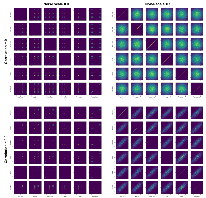
Figure 7: Visualization of the various distributions over latents. For 4 combinations of correlation levels and noise levels, we show the 2-dimensional histograms of samples from the corresponding distribution over latents described in Section D.2.1. Each histogram shows the joint distribution over two latent factors.

D.2.2 Metrics

We evaluate disentanglement via the mean correlation coefficient (Hyvärinen & Morioka, 2016; Khemakhem et al., 2020a) which is computed as follows: The Pearson correlation matrix $C$ between the ground-truth features and learned ones is computed. Then, $\text{MCC}=\max_{\pi\in\text{permutations}}\frac{1}{m}\sum_{j=1}^{m}|C_{j,\pi(j)}|$. We also evaluate linear equivalence by performing linear regression to predict the ground-truth factors from the learned ones, and report the mean of the Pearson correlations between the ground-truth latents and the learned ones. This metric is known as the coefficient of multiple correlations, $R$, and turns out to be the square-root of the more widely known coefficient of determination, $R^{2}$. The advantage of using $R$ over $R^{2}$ is that we always have $\text{MCC}\leq R$.

D.2.3 Architecture, inner solver & hyperparameters

We use the four-layer convolutional neural network typically used in the disentanglement literature (Locatello et al., 2019). As mentioned in Section 3.4, the norm of the representation ${\bm{f}}_{\hat{\bm{\theta}}}({\bm{x}})$ must be controlled to make sure the regularization remains effective. To do so, we apply batch normalization (Ioffe & Szegedy, 2015) at the very last layer of the neural network and do not learn its scale and shift parameters. Empirically, we do see the expected behavior that, without any normalization, the norm of ${\bm{f}}_{\hat{\bm{\theta}}}({\bm{x}})$ explodes as we train, leading to instabilities and low sparsity.

In these experiments, the distribution $p(y;\bm{\eta})$ used for learning is a Gaussian with fixed variance. In that case, the inner problem of Section 3.4 reduces to Lasso regression. Computing the hypergradient w.r.t. ${\bm{\theta}}$ requires solving this inner problem. To do so, we use Proximal Coordinate Descent (Tseng, 2001; Richtárik & Takáč, 2014).

Details on $\lambda/\lambda_{\max}$. In Fig. 4 and 6, we explore various levels of regularization $\lambda$. In our implementation, we set $\lambda=\epsilon\lambda_{\max}$ where $\epsilon\geq 0$. In inner-Lasso, we set $\lambda_{\max}:=\frac{1}{n}\lVert{\bm{F}}^{\top}{\bm{y}}\rVert_{\infty}$ (${\bm{F}}\in{\mathbb{R}}^{n\times m}$ is the design matrix of the features of the samples of a task), while in inner-Ridge we have $\lambda_{\max}:=\frac{1}{n}\lVert{\bm{F}}\rVert^{2}$. Note that this means $\lambda$ is dynamically changing as we train because ${\bm{F}}$ changes. However we never backpropagate through $\lambda_{\max}$ (we block the gradient from flowing). Thus, in all figures, we report $\epsilon=\lambda/\lambda_{\max}$.

D.2.4 Experiments violating assumptions

In this section, we explore variations of the experiments of Section 5, but this time the assumptions of Theorem 3.1 are violated.

Fig. 8 shows different degrees of violation of Assumption 3.6. We consider the cases where ${\mathcal{S}}:=\{\{1,2\},\{3,4\},\{5,6\}\}$ (block size = 2), ${\mathcal{S}}:=\{\{1,2,3\},\{4,5,6\}\}$ (block size = 3) and ${\mathcal{S}}:=\{\{1,2,3,4,5,6\}\}$ (block size = 6). Note that the latter case corresponds to having no sparsity at all in the ground-truth model, i.e., all tasks require all features. The reader can verify that these three cases indeed violate Assumption 3.6. In all cases, the distribution $p(S)$ puts uniform mass over its support ${\mathcal{S}}$. Similarly to the experiments from the main text, ${\bm{w}}:=\bar{{\bm{w}}}\odot{\bm{s}}$, where $\bar{\bm{w}}\sim\mathcal{N}({\bm{0}},{\bm{I}})$ and ${\bm{s}}\sim p(S)$ (${\bm{s}}$ is the binary representation of the set $S$). Overall, we can see that inner-Lasso does not perform as well when Assumption 3.6 is violated. For example, when there is no sparsity at all (block size = 6), inner-Lasso performs poorly and is even surpassed by inner-Ridge. Nevertheless, for mild violations (block size = 2), disentanglement (as measured by MCC) remains reasonably high. We further notice that all methods obtain very good R score in all settings. This is expected in light of Theorem B.4, which guarantees identifiability up to linear transformation without requiring Assumption 3.6.

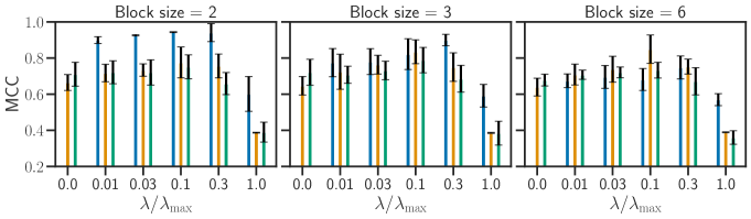
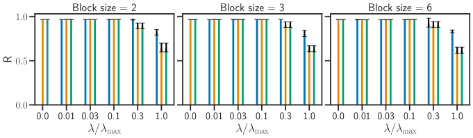
Figure 8: Disentanglement (MCC, top) and prediction (R Score, bottom) performances for inner-Lasso, inner-Ridge and inner-Ridge combined with ICA as a function of the regularization parameter. The metrics are plotted for multiple value of block size for the support. Block size $=6$ corresponds to no sparsity in the ground truth coefficients.

Fig. 9 presents experiments that are identitical to those of Fig. 4 in the main text, except for how ${\bm{w}}$ is generated. Here, the components of ${\bm{w}}$ are sampled independently according to ${\bm{w}}_{i}\sim\mathrm{Laplace}(\mu=0,b=1)$. We note that, under this process, the probability that ${\bm{w}}_{i}=0$ is zero. This means all features are useful and Assumption 3.6 is violated. That being said, due to the fat tail behavior of the Laplacian distribution, many components of ${\bm{w}}$ will be close to zero (relatively to its variance). Thus, this can be thought of as a weaker form of sparsity where many features are relatively unimportant. Fig. 9 shows that inner-Lasso can still disentangle very well. In fact, the performance is very similar to the experiments that presented actual sparsity (Fig. 4).

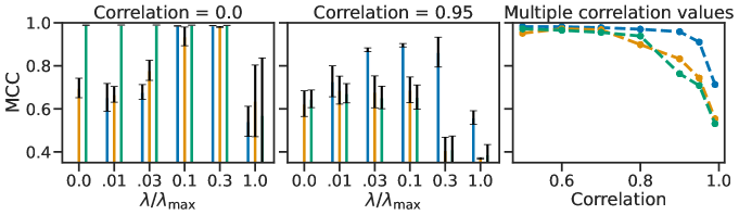
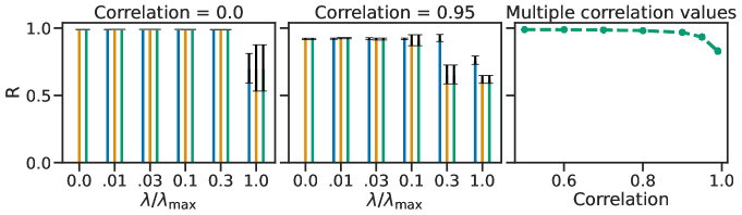
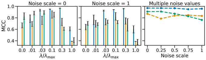
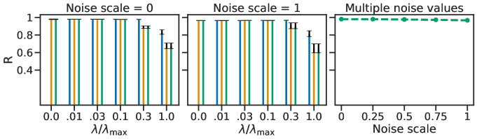
Figure 9: Same experiment as Fig. 4, but the task coefficient vectors ${\bm{w}}$ are sampled from a Laplacian distribution (instead of what was described in Section D.2.1). Performance is barely affected, showing some amount of robustness to violations of Assumption 3.6.

D.2.5 Experiments with regularization in the outer problem

Theorem B.6 presented an alternative optimization problem to that of Theorem 3.1 to learn a disentangled representation. Section B.3 presented a tractable relaxation of this alternative. The essential operational difference is that the sparsity regulatization appears in the outer problem instead of the inner problem. Figure 10 shows this alternative works as well empirically. Details in the caption.

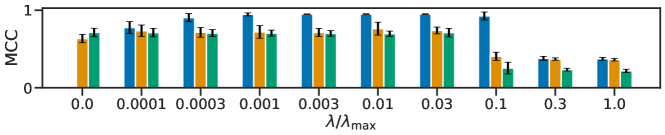
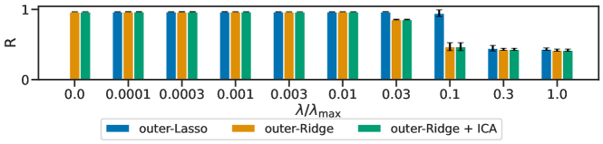
Figure 10: outer-Lasso solves Equation 60 (with regularization in the outer problem) while outer-Ridge solves the same problem but with an $L_{2}$-norm instead of $L_{2,1}$. The method outer-Ridge + ICA is outer-Ridge with an additional step of linear ICA on top of the learned representation. The results obtained are very similar to the main results of Fig. 4 and 6. In this dataset, the latents are sampled from $p_{\alpha=1,\rho=0.9}({\bm{z}})$ (See Section D.2.1) and the weight coefficients are sampled from the binomial-Gaussian process described in Section D.2.1.

D.2.6 Visual evaluation

Fig. 11, 12, 13 and 14 show how various learned representations respond to changing a single factor of variation in the image (Higgins et al., 2017, Figure 7.A.B). We see what was expected: the higher the MCC, the more disentangled the learned features appear, thus validating MCC as a good metric for disentanglement. See captions for details.

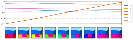
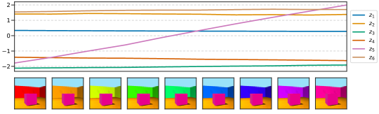
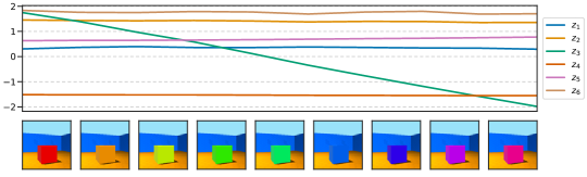
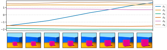
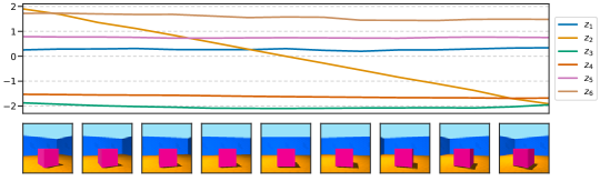
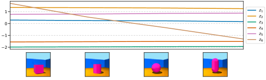
Figure 11: Varying one factor at a time in the image and showing how the learned representation varies in response. This representation was learned by inner-Lasso (best hyperparameter) on a dataset with 0 correlation between latents and a noise scale of 1. The corresponding MCC is 0.99. We can see that varying a single factor in the image always result in changing a single factor in the learned representation.

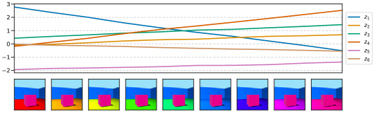
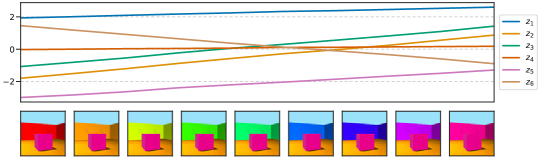
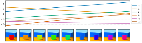
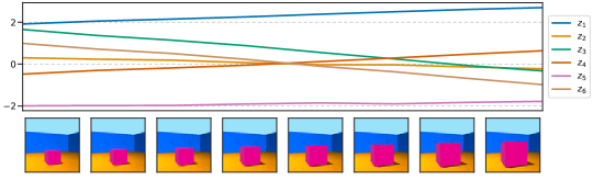
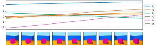
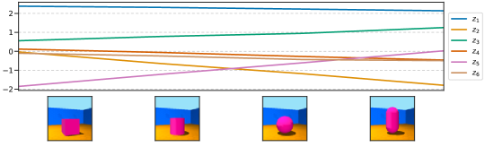
Figure 12: Varying one factor at a time in the image and showing how the learned representation varies in response. This representation was learned without regularization of any kind (i.e., with inner-Ridge with regularization coefficient equal to zero) on a dataset with 0 correlation between and a noise scale of 1. The corresponding MCC is 0.63. We can see that varying a single factor in the image result in changing multiple factors in the learned representation, i.e., the representation is not disentangled.

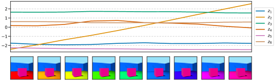
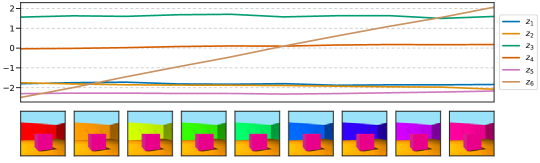
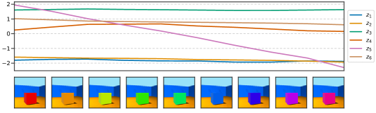
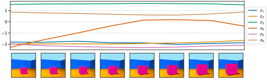
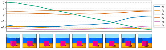
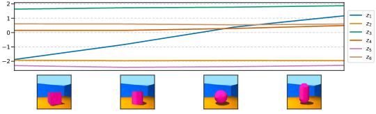
Figure 13: Varying one factor at a time in the image and showing how the learned representation varies in response. This representation was learned with inner-Lasso (best hyperparameter) on a dataset with correlation 0.9 between latents and a noise scale of 1. The corresponding MCC is 0.96. Qualitatively, the representation appears to be well disentangled, but not as well as in Fig. 11 (reflected by a drop in MCC of 0.03).

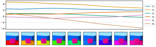
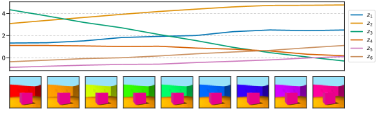
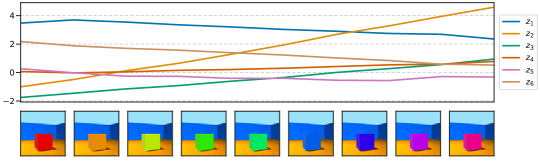
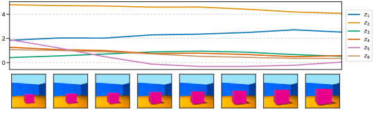
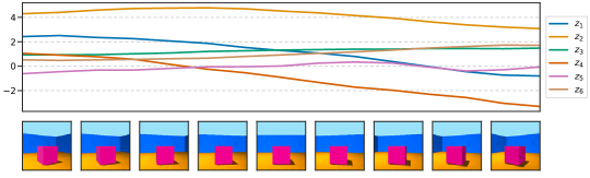
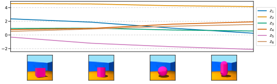
Figure 14: Varying one factor at a time in the image and showing how the learned representation varies in response. This representation was learned with inner-Ridge (best hyperparameter) on a dataset with correlation 0.9 between latents and a noise scale of 1. The corresponding MCC is 0.79. For most latent factors, we cannot identify a dominant feature, except maybe for background and object colors. The representation appears more disentangled than Fig. 12, but less disentangled than Fig. 13, as reflected by their corresponding MCC values.

D.2.7 Additional metrics for disentanglement

We implemented metrics from the DCI framework (Eastwood & Williams, 2018) to evaluate disentanglement. 1) DCI-Disentanglement: How many ground truth latent components are related to a particular component of the learned latent representation; 2) DCI-Completeness: How many learned latent components are related to a particular component of the ground truth latent representation. Note that for the definition of disentanglement used in the present work Definition 1.1, we want both DCI-disentanglement and DCI-completeness to be high.

The DCI framework requires a matrix of relative importance. In our implementation, this matrix is the coefficient matrix resulting from performing linear regression with inputs as the learned latent representation ${\bm{f}}_{\hat{\bm{\theta}}}({\bm{x}})$ and targets as the ground truth latent representation ${\bm{f}}_{{\bm{\theta}}}({\bm{x}})$, and denote the solution as the matrix $W$. Further, denote by $I=|W|$ as the importance matrix, as $I_{i,j}$ denotes the relevance of inferred latent ${\bm{f}}_{\hat{\bm{\theta}}}({\bm{x}})_{j}$ for predicting the true latent ${\bm{f}}_{{\bm{\theta}}}({\bm{x}})_{i}$.

Now, for computing DCI-disentanglement, we normalize each row of the importance matrix $I[i,:]$ by its sum so that it represents a probability distribution. Then disentanglement is given by $\frac{1}{m}\times\sum_{i}^{m}1-H(I[i,:])$, where $H$ denotes the entropy of a distribution. Note that for the desired case of each ground truth latent component being explained by a single inferred latent component, we would have $H(I[i,:])=0$ as we have a one-hot vector for the probability distribution. Similarly, for the case of each ground truth latent component being explained uniformly by all the inferred latents, $H(I[i,:])$ would be maximized and hence the DCI score would be minimized. To compute the DCI-completeness, we first normalize each column of the importance matrix $I[:,j]$ by its sum so that it represents a probability distribution and then compute $\frac{1}{m}\times\sum_{i}^{m}1-H(I[:,j])$.

Figure 15 shows the results for the 3D Shapes experiments (Section  5) with the DCI metric to evaluate disentanglement. Notice that we find the same trend as we had with the MCC metric 4, that inner-Lasso is more robust to correlation between the latent variables, and inner-Ridge + ICA performance drops down significantly with increasing correlation.

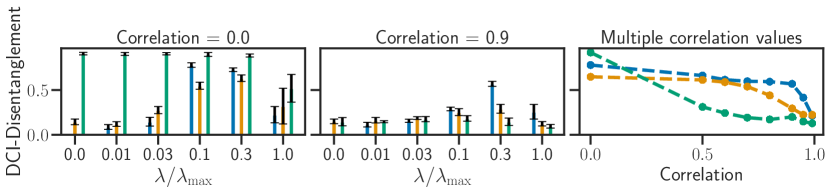
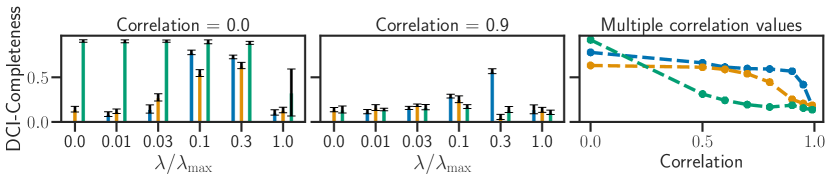
Figure 15: Disentanglement performance (DCI) for inner-Lasso, inner-Ridge and inner-Ridge combined with ICA as a function of the regularization parameter (left and middle). The right columns shows performance of the best hyperparameter for different values of correlation and noise. The top row shows the results for the disentanglement metric of DCI and the bottom row shows the results for the completeness metric of DCI.

D.3 Meta-learning experiments

Experimental settings. We evaluate the performance of our meta-learning algorithm based on a group-sparse SVM learners on the miniImageNet (Vinyals et al., 2016) dataset. Following the standard nomenclature in few-shot classification (Hospedales et al., 2021) with $k$-shot $N$-way, where $N$ is the number of classes in each classification task, and $k$ is the number of samples per class in the training dataset ${\mathcal{D}}_{t}^{\mathrm{train}}$, we consider the experimental setting $5$-shot $5$-way. We use the same residual network architecture as in (Lee et al., 2019), with $12$ layers and a representation of size $p=1.6\times 10^{4}$.

Technical details. The objective of Equation 8 is composed of a smooth term and block separable non-smooth term, hence it can be solved efficiently using proximal block coordinate descent (Tseng, 2001). Although Theorem 3.1 is not directly applicable to the meta-learning formulation proposed in this section, we conjecture that similar techniques could be reused to prove an identifiability result in this setting. As in Section 3.4, the argmin differentiation of the solution of Equation 8 can be done using implicit differentiation (Bertrand et al., 2022).

References

- Ahuja et al. (2020) Ahuja, K., Shanmugam, K., Varshney, K. R., and Dhurandhar, A. Invariant risk minimization games. In Proceedings of the 37th International Conference on Machine Learning, 2020.
- Ahuja et al. (2022a) Ahuja, K., Hartford, J., and Bengio, Y. Properties from mechanisms: an equivariance perspective on identifiable representation learning. In International Conference on Learning Representations, 2022a.
- Ahuja et al. (2022b) Ahuja, K., Hartford, J., and Bengio, Y. Weakly supervised representation learning with sparse perturbations, 2022b.
- Ahuja et al. (2022c) Ahuja, K., Mahajan, D., Syrgkanis, V., and Mitliagkas, I. Towards efficient representation identification in supervised learning. In First Conference on Causal Learning and Reasoning, 2022c.
- Argyriou et al. (2008) Argyriou, A., Evgeniou, T., and Pontil, M. Convex multi-task feature learning. Machine learning, 73(3):243–272, 2008.
- Arjovsky et al. (2020) Arjovsky, M., Bottou, L., Gulrajani, I., and Lopez-Paz, D. Invariant risk minimization, 2020.
- Ba et al. (2016) Ba, J. L., Kiros, J. R., and Hinton, G. E. Layer normalization. arXiv preprint arXiv:1607.06450, 2016.
- Bengio (2000) Bengio, Y. Gradient-based optimization of hyperparameters. Neural computation, 12(8):1889–1900, 2000.
- Bengio et al. (2013) Bengio, Y., Courville, A., and Vincent, P. Representation learning: A review and new perspectives. IEEE transactions on pattern analysis and machine intelligence, 2013.
- Bertinetto et al. (2019) Bertinetto, L., Henriques, J. F., Torr, P. H., and Vedaldi, A. Meta-learning with differentiable closed-form solvers. 2019.
- Bertrand et al. (2020) Bertrand, Q., Klopfenstein, Q., Blondel, M., Vaiter, S., Gramfort, A., and Salmon, J. Implicit differentiation of lasso-type models for hyperparameter optimization. In International Conference on Machine Learning, pp. 810–821. PMLR, 2020.
- Bertrand et al. (2022) Bertrand, Q., Klopfenstein, Q., Massias, M., Blondel, M., Vaiter, S., Gramfort, A., and Salmon, J. Implicit differentiation for fast hyperparameter selection in non-smooth convex learning. JMLR, 2022.
- Bickel et al. (2009) Bickel, P. J., Ritov, Y., and Tsybakov, A. B. Simultaneous analysis of lasso and Dantzig selector. The Annals of statistics, 37(4):1705–1732, 2009.
- Blondel et al. (2022) Blondel, M., Berthet, Q., Cuturi, M., Frostig, R., Hoyer, S., Llinares-López, F., Pedregosa, F., and Vert, J.-P. Efficient and modular implicit differentiation. NeurIPS, 2022.
- Bolte et al. (2021) Bolte, J., Le, T., E., Pauwels, and Silveti-Falls, T. Nonsmooth implicit differentiation for machine-learning and optimization. Advances in neural information processing systems, 34:13537–13549, 2021.
- Bolte et al. (2022) Bolte, J., Pauwels, E., and Vaiter, S. Automatic differentiation of nonsmooth iterative algorithms. NeurIPS, 2022.
- Bouchacourt et al. (2018) Bouchacourt, D., Tomioka, R., and Nowozin, S. Multi-level variational autoencoder: Learning disentangled representations from grouped observations. Proceedings of the AAAI Conference on Artificial Intelligence, 2018.
- Boyd et al. (2004) Boyd, S. P., , and Vandenberghe, L. Convex optimization. Cambridge university press, 2004.
- Bradbury et al. (2018) Bradbury, J., Frostig, R., Hawkins, P., Johnson, M. J., Leary, C., Maclaurin, D., Necula, G., Paszke, A., VanderPlas, J., Wanderman-Milne, S., and Zhang, Q. JAX: composable transformations of Python+NumPy programs, 2018. URL http://github.com/google/jax.
- Brehmer et al. (2022) Brehmer, J., De Haan, P., Lippe, P., and Cohen, T. Weakly supervised causal representation learning. In Advances in Neural Information Processing Systems, 2022.
- Brown et al. (2020a) Brown, T., Mann, B., Ryder, N., Subbiah, M., Kaplan, J. D., Dhariwal, P., Neelakantan, A., Shyam, P., Sastry, G., Askell, A., Agarwal, S., Herbert-Voss, A., Krueger, G., Henighan, T., Child, R., Ramesh, A., Ziegler, D., Wu, J., Winter, C., Hesse, C., Chen, M., Sigler, E., Litwin, M., Gray, S., Chess, B., Clark, J., Berner, C., McCandlish, S., Radford, A., Sutskever, I., and Amodei, D. Language models are few-shot learners. In Advances in Neural Information Processing Systems, 2020a.
- Brown et al. (2020b) Brown, T., Mann, B., Ryder, N., Subbiah, M., Kaplan, J. D., Dhariwal, P., Neelakantan, A., Shyam, P., Sastry, G., Askell, A., et al. Language models are few-shot learners. Advances in Neural Information Processing Systems, 33:1877–1901, 2020b.
- Burgess & Kim (2018) Burgess, C. and Kim, H. 3d shapes dataset. https://github.com/deepmind/3dshapes-dataset/, 2018.
- Casella & Berger (2001) Casella, G. and Berger, R. Statistical Inference. Duxbury Resource Center, 2001.
- Chen et al. (2018) Chen, R. T. Q., Li, X., G., R., and Duvenaud, D. Isolating sources of disentanglement in vaes. In Advances in Neural Information Processing Systems, 2018.
- Chen et al. (1998) Chen, S. S., Donoho, D. L., and Saunders, M. A. Atomic decomposition by basis pursuit. SIAM Journal on Scientific Computing, 1998.
- Chen et al. (2020) Chen, T., Kornblith, S., Norouzi, M., and Hinton, G. A simple framework for contrastive learning of visual representations. In International Conference on Machine Learning, pp. 1597–1607. PMLR, 2020.
- Comon (1992) Comon, P. Independent component analysis. Higher-Order Statistics, 1992.
- Crammer & Singer (2001) Crammer, K. and Singer, Y. On the algorithmic implementation of multiclass kernel-based vector machines. Journal of machine learning research, 2(Dec):265–292, 2001.
- Devlin et al. (2018) Devlin, J., Chang, M.-W., Lee, K., and Toutanova, K. Bert: Pre-training of deep bidirectional transformers for language understanding. arXiv preprint arXiv:1810.04805, 2018.
- Dittadi et al. (2021) Dittadi, A., Träuble, F., Locatello, F., Wuthrich, M., Agrawal, V., Winther, O., Bauer, S., and Schölkopf, B. On the transfer of disentangled representations in realistic settings. In International Conference on Learning Representations, 2021.
- Dosovitskiy et al. (2021) Dosovitskiy, A., Beyer, L., Kolesnikov, A., Weissenborn, D., Zhai, X., Unterthiner, T., Dehghani, M., Minderer, M., Heigold, G., Gelly, S., et al. An image is worth 16x16 words: Transformers for image recognition at scale. International Conference on Learning Representations, 2021.
- Duan et al. (2020) Duan, S., Matthey, L., Saraiva, A., Watters, N., Burgess, C., Lerchner, A., and Higgins, I. Unsupervised model selection for variational disentangled representation learning. In International Conference on Learning Representations, 2020.
- Eastwood & Williams (2018) Eastwood, C. and Williams, C. K. A framework for the quantitative evaluation of disentangled representations. In International Conference on Learning Representations, 2018.
- Finn et al. (2017) Finn, C., Abbeel, P., and Levine, S. Model-agnostic meta-learning for fast adaptation of deep networks. In International conference on machine learning, pp. 1126–1135. PMLR, 2017.
- Goyal & Bengio (2022) Goyal, A. and Bengio, Y. Inductive biases for deep learning of higher-level cognition. Proc. R. Soc. A 478: 20210068, 2022.
- Gresele et al. (2021) Gresele, L., Kügelgen, J. V., Stimper, V., Schölkopf, B., and Besserve, M. Independent mechanism analysis, a new concept? In Advances in Neural Information Processing Systems, 2021.
- Gribonval & Lesage (2006) Gribonval, R. and Lesage, S. A survey of sparse component analysis for blind source separation: principles, perspectives, and new challenges. In ESANN’06 proceedings - 14th European Symposium on Artificial Neural Networks, 2006.
- Higgins et al. (2017) Higgins, I., Matthey, L., Pal, A., Burgess, C. P., Glorot, X., Botvinick, M., Mohamed, S., and Lerchner, A. beta-vae: Learning basic visual concepts with a constrained variational framework. In ICLR, 2017.
- Hoerl & Kennard (1970) Hoerl, A. E. and Kennard, R. W. Ridge regression: Biased estimation for nonorthogonal problems. Technometrics, 12(1):55–67, 1970.
- Hospedales et al. (2021) Hospedales, T., Antoniou, A., Micaelli, P., and Storkey, A. Meta-learning in neural networks: A survey. IEEE transactions on pattern analysis and machine intelligence, 44(9):5149–5169, 2021.
- Hsieh et al. (2008) Hsieh, C.-J., Chang, K.-W., Lin, C.-J., Keerthi, S. S., and Sundararajan, S. A dual coordinate descent method for large-scale linear svm. In Proceedings of the 25th international conference on Machine learning, pp. 408–415, 2008.
- Hyvärinen & Morioka (2016) Hyvärinen, A. and Morioka, H. Unsupervised feature extraction by time-contrastive learning and nonlinear ica. In Advances in Neural Information Processing Systems, 2016.
- Hyvärinen & Morioka (2017) Hyvärinen, A. and Morioka, H. Nonlinear ICA of Temporally Dependent Stationary Sources. In Proceedings of the 20th International Conference on Artificial Intelligence and Statistics, 2017.
- Hyvärinen & Pajunen (1999) Hyvärinen, A. and Pajunen, P. Nonlinear independent component analysis: Existence and uniqueness results. Neural Networks, 1999.
- Hyvärinen et al. (2001) Hyvärinen, A., Karhunen, J., and Oja, E. Independent Component Analysis. Wiley, 2001.
- Hyvärinen et al. (2019) Hyvärinen, A., Sasaki, H., and Turner, R. E. Nonlinear ica using auxiliary variables and generalized contrastive learning. In AISTATS. PMLR, 2019.
- Ioffe & Szegedy (2015) Ioffe, S. and Szegedy, C. Batch normalization: Accelerating deep network training by reducing internal covariate shift. In Proceedings of the 32nd International Conference on Machine Learning, 2015.
- Khemakhem et al. (2020a) Khemakhem, I., Kingma, D., Monti, R., and Hyvärinen, A. Variational autoencoders and nonlinear ica: A unifying framework. In Proceedings of the Twenty Third International Conference on Artificial Intelligence and Statistics, 2020a.
- Khemakhem et al. (2020b) Khemakhem, I., Monti, R., Kingma, D., and Hyvärinen, A. Ice-beem: Identifiable conditional energy-based deep models based on nonlinear ica. In Advances in Neural Information Processing Systems, 2020b.
- Kim & Mnih (2018) Kim, H. and Mnih, A. Disentangling by factorising. In Proceedings of the 35th International Conference on Machine Learning, 2018.
- Klindt et al. (2021) Klindt, D. A., Schott, L., Sharma, Y., Ustyuzhaninov, I., Brendel, W., Bethge, M., and Paiton, D. M. Towards nonlinear disentanglement in natural data with temporal sparse coding. In 9th International Conference on Learning Representations, 2021.
- Kreutz-Delgado et al. (2003) Kreutz-Delgado, K., Murray, J. F., Rao, B. D., Engan, K., Lee, T.-W., and Sejnowski, T. J. Dictionary learning algorithms for sparse representation. Neural computation, 15(2):349–396, 2003.
- Krueger et al. (2021) Krueger, D., Caballero, E., Jacobsen, J.-H., Zhang, A., Binas, J., Priol, R. L., Zhang, D., and Courville, A. Out-of-distribution generalization via risk extrapolation ({re}x), 2021.
- Kumar et al. (2018) Kumar, A., Sattigeri, P., and Balakrishnan, A. Variational inference of disentangled latent concepts from unlabeled observations. In International Conference on Learning Representations, 2018.
- Lachapelle & Lacoste-Julien (2022) Lachapelle, S. and Lacoste-Julien, S. Partial disentanglement via mechanism sparsity. In UAI 2022 Workshop on Causal Representation Learning, 2022.
- Lachapelle et al. (2022) Lachapelle, S., Rodriguez Lopez, P., Sharma, Y., Everett, K. E., Le Priol, R., Lacoste, A., and Lacoste-Julien, S. Disentanglement via mechanism sparsity regularization: A new principle for nonlinear ICA. In First Conference on Causal Learning and Reasoning, 2022.
- Lee et al. (2019) Lee, K., S.Maji, Ravichandran, A., and Soatto, S. Meta-learning with differentiable convex optimization. In Proceedings of the IEEE/CVF conference on computer vision and pattern recognition, pp. 10657–10665, 2019.
- Lippe et al. (2022a) Lippe, P., Magliacane, S., Löwe, S., Asano, Y. M., Cohen, T., and Gavves, E. iCITRIS: Causal representation learning for instantaneous temporal effects. In UAI 2022 Workshop on Causal Representation Learning, 2022a.
- Lippe et al. (2022b) Lippe, P., Magliacane, S., Löwe, S., Asano, Y. M., Cohen, T., and Gavves, E. CITRIS: Causal identifiability from temporal intervened sequences, 2022b.
- Locatello et al. (2019) Locatello, F., Bauer, S., Lucic, M., Raetsch, G., Gelly, S., Schölkopf, B., and Bachem, O. Challenging common assumptions in the unsupervised learning of disentangled representations. In Proceedings of the 36th International Conference on Machine Learning, 2019.
- Locatello et al. (2020a) Locatello, F., Poole, B., Raetsch, G., Schölkopf, B., Bachem, O., and Tschannen, M. Weakly-supervised disentanglement without compromises. In Proceedings of the 37th International Conference on Machine Learning, 2020a.
- Locatello et al. (2020b) Locatello, F., Tschannen, M., Bauer, S., Rätsch, G., Schölkopf, B., and Bachem, O. Disentangling factors of variations using few labels. In International Conference on Learning Representations, 2020b. URL https://openreview.net/forum?id=SygagpEKwB.
- Lounici et al. (2011a) Lounici, K., Pontil, M., and Tsybakov, A. B. Oracle inequalities and optimal inference under group sparsity. The Annals of statistics, 2011a.
- Lounici et al. (2011b) Lounici, K., Pontil, M., Van De Geer, S., and Tsybakov, A. B. Oracle inequalities and optimal inference under group sparsity. The annals of statistics, 2011b.
- Lu et al. (2021) Lu, C., Wu, Y., Hernández-Lobato, J. M., and Schölkopf, B. Nonlinear invariant risk minimization: A causal approach, 2021.
- Mairal et al. (2008) Mairal, J., Ponce, J., Sapiro, G., Zisserman, A., and Bach, F. Supervised dictionary learning. Advances in neural information processing systems, 21, 2008.
- Mairal et al. (2009) Mairal, J., Bach, F., Ponce, J., and Sapiro, G. Online dictionary learning for sparse coding. In Proceedings of the 26th annual international conference on machine learning, pp. 689–696, 2009.
- Mairal et al. (2011) Mairal, J., Bach, F., and Ponce, J. Task-driven dictionary learning. IEEE transactions on pattern analysis and machine intelligence, 34(4):791–804, 2011.
- Malézieux et al. (2022) Malézieux, B., Moreau, T., and Kowalski, M. Dictionary and prior learning with unrolled algorithms for unsupervised inverse problems. ICLR, 2022.
- Marcus et al. (2022) Marcus, G., Davis, E., and Aaronson, S. A very preliminary analysis of dall-e 2. arXiv preprint arXiv:2204.13807, 2022.
- Maurer et al. (2013) Maurer, A., Pontil, M., and Romera-Paredes, B. Sparse coding for multitask and transfer learning. ICML’13, 2013.
- Maurer et al. (2016) Maurer, A., Pontil, M., and Romera-Paredes, B. The benefit of multitask representation learning. J. Mach. Learn. Res., 2016.
- Mikolov et al. (2010) Mikolov, T., Karafiát, M., Burget, L., Cernocký, J., and Khudanpur, S. Recurrent neural network based language model. ISCA, 2010.
- Miladinović et al. (2019) Miladinović, D., Gondal, M. W., Schölkopf, B., Buhmann, J. M., and Bauer, S. Disentangled state space representations. arXiv preprint arXiv:1906.03255, 2019.
- Mohri et al. (2018) Mohri, M., Rostamizadeh, A., and Talwalkar, A. MIT Press, 2018.
- Montero et al. (2021) Montero, M. L., Ludwig, C. J., Costa, R. P., Malhotra, G., and Bowers, J. The role of disentanglement in generalisation. In International Conference on Learning Representations, 2021.
- Moran et al. (2022) Moran, G. E., Sridhar, D., Wang, Y., and Blei, D. Identifiable deep generative models via sparse decoding. Transactions on Machine Learning Research, 2022.
- Oord et al. (2018) Oord, A., Li, Y., and Vinyals, O. Representation learning with contrastive predictive coding. Advances in Neural Information Processing Systems, 2018.
- Pearl (2019) Pearl, J. The seven tools of causal inference, with reflections on machine learning. Commun. ACM, 2019.
- Pedregosa (2016) Pedregosa, F. Hyperparameter optimization with approximate gradient. In International conference on machine learning, pp. 737–746. PMLR, 2016.
- Radford et al. (2021) Radford, A., Kim, J. W., Hallacy, C., Ramesh, A., Goh, G., Agarwal, S., Sastry, G., Askell, A., Mishkin, P., Clark, J., et al. Learning transferable visual models from natural language supervision. In International Conference on Machine Learning, pp. 8748–8763. PMLR, 2021.
- Ramesh et al. (2022) Ramesh, A., Dhariwal, P., Nichol, A., Chu, C., and Chen, M. Hierarchical text-conditional image generation with clip latents. arXiv preprint arXiv:2204.06125, 2022.
- Richtárik & Takáč (2014) Richtárik, P. and Takáč, M. Iteration complexity of randomized block-coordinate descent methods for minimizing a composite function. Mathematical Programming, 144(1):1–38, 2014.
- Roeder et al. (2021) Roeder, G., Metz, L., and Kingma, D. P. On linear identifiability of learned representations. In Proceedings of the 38th International Conference on Machine Learning, 2021.
- Schölkopf et al. (2021) Schölkopf, B., Locatello, F., Bauer, S., Ke, N. R., Kalchbrenner, N., Goyal, A., and Bengio, Y. Toward causal representation learning. Proceedings of the IEEE - Advances in Machine Learning and Deep Neural Networks, 2021.
- Schölkopf (2019) Schölkopf, B. Causality for machine learning, 2019.
- Snell et al. (2017) Snell, J., Swersky, K., and Zemel, R. Prototypical networks for few-shot learning. Advances in Neural Information Processing Systems, 30, 2017.
- Taleb & Jutten (1999) Taleb, A. and Jutten, C. Source separation in post-nonlinear mixtures. IEEE Transactions on Signal Processing, 1999.
- Tibshirani (1996) Tibshirani, R. Regression shrinkage and selection via the lasso. Journal of the Royal Statistical Society: Series B (Methodological), 58(1):267–288, 1996.
- Tseng (2001) Tseng, P. Convergence of a block coordinate descent method for nondifferentiable minimization. Journal of optimization theory and applications, 109(3):475–494, 2001.
- van Steenkiste et al. (2019) van Steenkiste, S., Locatello, F., Schmidhuber, J., and Bachem, O. Are disentangled representations helpful for abstract visual reasoning? In Advances in Neural Information Processing Systems, 2019.
- Vinyals et al. (2016) Vinyals, O., Blundell, C., Lillicrap, T., Wierstra, D., et al. Matching networks for one shot learning. Advances in neural information processing systems, 29, 2016.
- Von Kügelgen et al. (2021) Von Kügelgen, J., Sharma, Y., Gresele, L., Brendel, W., Schölkopf, B., Besserve, M., and Locatello, F. Self-supervised learning with data augmentations provably isolates content from style. In Thirty-Fifth Conference on Neural Information Processing Systems, 2021.
- Wainwright & Jordan (2008) Wainwright, M. J. and Jordan, M. I. Graphical models, exponential families, and variational inference. Found. Trends Mach. Learn., 2008.
- Wortsman et al. (2022) Wortsman, M., Ilharco, G., Kim, J. W., Li, M., Kornblith, S., Roelofs, R., Lopes, R. G., Hajishirzi, H., Farhadi, A., Namkoong, H., and Schmidt, L. Robust fine-tuning of zero-shot models. In Proceedings of the IEEE/CVF Conference on Computer Vision and Pattern Recognition (CVPR), pp. 7959–7971, June 2022.
- Wright & Nocedal (1999) Wright, S. and Nocedal, J. Numerical optimization. Springer Science, 35(67-68):7, 1999.
- Yao et al. (2022) Yao, W., Sun, Y., Ho, A., Sun, C., and Zhang, K. Learning temporally causal latent processes from general temporal data. In International Conference on Learning Representations, 2022.
- Zhang et al. (2022) Zhang, H., Zhang, Y.-F., Liu, W., Weller, A., Schölkopf, B., and Xing, E. Towards principled disentanglement for domain generalization. In Proceedings of the IEEE/CVF Conference on Computer Vision and Pattern Recognition (CVPR), 2022.
- Zheng et al. (2022) Zheng, Y., Ng, I., and Zhang, K. On the identifiability of nonlinear ICA: Sparsity and beyond. In Advances in Neural Information Processing Systems, 2022.