Iterated Function Systems:
A Comprehensive Survey
Abstract
We provide an overview of iterated function systems (IFS), where randomly chosen state-to-state maps are iteratively applied to a state. We aim to summarize the state of art and, where possible, identify fundamental challenges and opportunities for further research.
1 Introduction
The fundamental mathematical tool used in this study is discrete-time Markov chains, which are generated by random repetition of functions and exhibit long-term statistical behaviour. Allow us to encourage readers through an example from (Chakraborty,, 2016, Section 2.1, Chapter 1); similar examples could be found in (Barnsley,, 1993, Chapter 3). Assume a particle is located at the origin, i.e., at of a two-dimensional Euclidean plane. Consider a die with four sides denoted by the integers . The particle moves on the plane according to rules as shown in Table 1:
| A number appears in the dice | Where the particle moves |
|---|---|
Initially, the particle is at ; now, imagine shows up after throwing the die. From the rules described in the table, the particle will move to where is its current coordinate. For us, the initial position of the particle, and since has appeared, the next position or co-ordinate of the particle is
We mark the point with a pen. We throw the die again, and depending on the number, and the particle moves to a different point from . If we repeat these steps for, say, times (Of course, that requires the help of a computer) and mark those points on the plane, we get a picture similar to Figure 1.
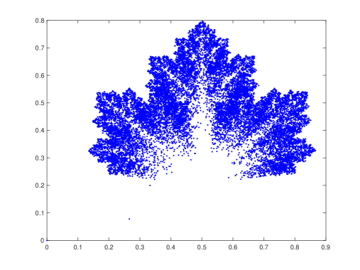
These points visited by the particle are insufficient to cover all points in the leaf and produce a fully formed naturally shaped leaf devoid of holes. After several iterations, a two-dimensional maple leaf is the particle’s sole visited or so-called accessible position. One may demonstrate that with probability one, the sequence of points , referred to as a sample path or trajectory, would ultimately pass through any portion of the Maple leaf. The exciting aspect of the game is that even though the particle’s travel was random in each step, the movement’s long-term behaviour took on the form of a Maple leaf. The outcome will be the same regardless of how many individuals play the game concurrently or how many times. Particular emphasis should be placed on the terms “with probability one”, which will be explained subsequently. The trajectory will approach the same point if the dice consistently display the same face. However, for a fair dice, this occurrence has zero chance. The act of continually tossing the dice is referred to as “iteration”, and the rule dictating how the particle should advance to the next step from the present position is known as a “function”. It could be easily seen that the four rules described in the table above can be seen as the following functions acting on as follows:
The chaotic game seen above illustrates the “random repetition of functions” (where the randomness appeared due to the throwing of the die).
1.1 Some Motivating Applications of IFS
Example 1.1.
Non-linear time series in Statistics: A first-order autoregression model is defined in non-linear time series analysis as
is critical in time series analysis because it represents a strong (i.i.d.) white noise sequence. Establishing the requirements for a stationary solution to the first-order autoregressive equation is simple. A nearly comparable process is provided by
| (1) |
where is a series of independently generated random vectors in . These models are critical in non-linear time series modelling. The presence of strict-sense and weak-sense stable solutions to the equation (1) is a natural issue. Under certain weak circumstances, (Douc et al.,, 2014, Theorem 4.1) established the existence of strict-sense stationery. The theorem has been further generalized to functional autoregressive process using IFS techniques (Douc et al.,, 2014, Theorem 4.40, 4.41) and based on these results, a weak-sense stationary solution to (1) has been shown in (Douc et al.,, 2014, Theorem 4.47) under the assumptions (Douc et al.,, 2014, Assumption A4.43-A4.45).
Example 1.2.
IFS in finance: Uniquely ergodic IFS with constant probability are valuable alternatives to the standard binomial models (see Van der Hoek and Elliott, (2006)) of stock price development that are used to estimate one-period option pricing (Swishchuk and Islam,, 2013, Section 3.8). A generalised binomial model Cox et al., (1979) is found using IFS with state-dependent probability for call option prices, bond valuation, stock price evolution, and interest rates. See (Swishchuk and Islam,, 2013, Section 4.6.1, 4.6.4) and (Bahsoun et al., 2005b, ).
Example 1.3.
Stability of congestion management, e.g., in Transmission Control Protocol: The distribution of limited resources among several agents in different scientific fields and applications is one of the most challenging problems. For example, the bandwidth available for communication on computer networks is limited. Each connection can simultaneously support several data flows, each seeking to optimize its portion of the available bandwidth. A circumstance like that occurs when many electric cars are charged concurrently at the same charging station and compete for the same electricity or charge rate. A scalable and robust solution to this challenge is required. Additionally, a decentralized technique is appropriate when there is limited interaction between users and maintaining anonymity is critical. The method additive increase and multiplicative decrease (AIMD) has been quite effective in resolving the issue (Chiu and Jain,, 1989). In actuality, a more complex and challenging scenario occurs. To address such scenarios, the stochastic linear AIMD method and the stochastic additive increase and non-linear decrease (AINLD) algorithm developed in (Corless et al.,, 2016, Chapter 6, 7, 8) have been extensively investigated utilizing IFS and their ergodic features. For example, in (Corless et al.,, 2016, Chapter 7) the AIMD with state-dependent transition probabilities has been modelled as
| (2) |
where is vector-valued random variable and defined as
where for each , is the amount of share consumed by the user and represents discrete time instants, represent the overall capacity of the resource accessible to the whole system, and is assumed for the purpose of easy computation, AIMD matrix is given by
where is the rate of growth of the agent after the capacity event (a time when the resource reaches its capacity constraint, i.e., ) and denote multiplicative decrease quantity at the capacity event depending on the response of the user at the capacity event, .
It can be shown that the AIMD matrices are non-negative, column stochastic. The set of matrices arising through (2) is denoted by finite set of indices and . The technique is stochastic because the index is created randomly for each event ; that is, is a random variable. Thus,
The equation (2) may be used to represent the dynamical system of interest in the networks of AIMD flows. We refer to a state-dependent AIMD model in the paper (Corless et al.,, 2016, Chapter 7).
Consider as a collection of probability functions from the simplex into the closed interval that fulfil
Here, denotes the probability that the matrix occurs when the state or the share vector is , i.e.,
| (3) |
or,
| (4) |
Take note that (3) and (4) create a stochastic AIMD algorithm, and they are an IFS with the state (or place) dependent probabilities, and more precisely, a Markov chain on , whose state transition probabilities are provided by
| (5) |
Having created AIMD’s mathematical framework, we may question how the AIMD algorithm distributes resources efficiently among the participants. Can the algorithm ensure equal shares for all network agents? Several other relevant research questions are highlighted in (Corless et al.,, 2016, Chapter 1, Section 1.4). To know more about this direction please see Dumas et al., (2002); Wirth et al., 2006b ; Shorten et al., (2007); Wirth et al., 2006a ; King and Shorten, (2006); Shorten et al., (2007); Corless and Shorten, 2012a ; Corless and Shorten, 2012b ; Fioravanti et al., (2017, 2019); Crisostomi et al., (2016); Corless et al., (2016); Epperlein and Mareček, (2017); Wirth et al., (2019); Leśniak et al., (2021); Ghosh et al., (2022).
Example 1.4.
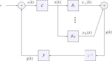
Closed-loop models within sharing economy: Imagine if an number of agent-based system with with a controller , filter , in a closed-loop feedback as in Figure 2. At time , generates a signal . As a result, agents adjust the way they utilize the resource. Due to unpredictability in the agent’s reaction to the control signal, randomized control signal, or random perturbations of the control signal, for all , the agent’s state at time is treated as a random variable, and we note that has no access to or but only able to get access to the error signal , which indicates a difference between the value that is produced by the filter and the desired output value . Smart grid and smart city applications may be shown with this simple setup. In this closed-loop feedback system, a stochastic difference equation governs the state of each agent:
| (6) |
where are taken as general response functions of agents in the network, are valued independent identically distributed (i.i.d) discrete random variables. This representation is precisely an IFS system.
The controller and filter take all conceivable initial state distributions into account to guarantee that the system’s long-term behaviour is acceptable for all agents involved. For each stable linear controller and filter, we seek conditions where the feedback loop controls total resource consumption and converges to a unique invariant measure. The above concept and strategy have been investigated in a variety of other engineering fields, including smart-city and smart-grid control (Fioravanti et al.,, 2017, 2019), congestion control (Shorten et al.,, 2005), resource allocation (Epperlein and Mareček,, 2017), load aggregation and operation of virtual power plants (Marecek et al.,, 2021), social sensing platforms (Ghosh et al.,, 2022), and model predictive control (Kungurtsev et al.,, 2021).
Example 1.5.
Opinion dynamics: There has long been a focus of research at the junction of economics and dynamical systems; for example, Acemoglu’s pioneering work utilizing IFS Acemoglu et al., (2010); Acemoğlu et al., (2013), and the references therein. The Friedkin-Johnsen model Friedkin and Johnsen, (2011) accurately depicts opinion dynamics characterized by heterogeneity. Wei et al., (2019) shown that the Friedkin-Johnsen model is a specific example of their expanded Rescorla-Wagner model Rescorla, (1972). Surprisingly, this extended model with random time-varying topology is exactly a recurrent IFS, and the suggested model’s internal states exhibit both convergence and ergodicity.
Example 1.6.
Stochastic dynamic decision model: Following (Hinderer,, 1970, Chapter 1), let a set be called the state space, and let be another set called action space. Let is a sequence of maps from certain sets or ( factors), according as or , into the class of all non-empty subsets of such that
is called the set of histories at time , the set of all admissible histories at time , and the set of all admissible actions at time under admissible history . Denoting we can write . Let be a probability distribution on called the initial distribution and is a transition probability function from to , i.e. for any , is a probability distribution on , called transition law from time to . And, finally, let is an extended real-valued function on called reward during the time interval . A collection with the above properties is called a stochastic dynamic decision model. Choosing a policy and an optimality criterion is necessary to define a dynamic optimisation problem under the suitable assumption on . A deterministic admissible policy is of maps such that
where
denotes the history at time obtained when the sequence of states occurred and actions were chosen according to . The application of a policy generates a stochastic process, the decision process determined by , is as follows: Starting at some at some point , selected from according to the initial probability distribution , one takes action whereupon one gets the reward , and the system moves to some selected according to . Then the action is taken, giving the and the system moves to some selected according to and so on. Thus for a given policy, the sequence of states then appears equivalent to the IFS.
Example 1.7.
In DNA replication model: The DNA replication kinetic equation is shown in (Gaspard,, 2017, Equation 2). New DNA strands are created by molecular machinery utilizing templates from previous generations. To correctly solve replication kinetic equations, one may use iterative function systems that run along the template sequence and provide copy sequence statistics and kinetic and thermodynamic parameters. DNA polymerase local velocity distributions with fractal and continuous sequence heterogeneity are studied using this approach, as well as the transition between linear and sub-linear copy growth rates.
1.2 Organization of the Survey and Past Surveys on IFS
Our survey is organized as follows: Sections 3–6 survey key research areas within the current IFS literature. Section 7 of the survey focuses on structural results, which can be seen as the geometry of the unique invariant measure. Finally, Section 8 highlights several possible research directions. In Figure 3, 4 and 5, we have broken down the key areas to ease navigating the survey. In the appendices, we provide pointers to key papers witihin applications of IFS.
We should also like to point to the excellent and well-known surveys of Diaconis and Freedman, (1999), and Iosifescu, (2009), and the lesser-known surveys and reviews of Kaijser, (1981); Stenflo, 2012b ; Stenflo, 1998b ; Letac et al., (1986); Chamayou and Letac, (1991); Carlsson, 2005a ; Bhattacharya and Majumdar, (2003); Athreya, 2003b ; Athreya, (2016); Fuh, (2004); Majumdar, (2009); Kunze et al., (2011); Denker and Waymire, (2016). For a survey on a random iteration of quadratic functions, see Athreya and Bhattacharya, (2001). The sheer fact that our survey appears more than two decades after Diaconis and Freedman, (1999) makes it possible to cover more of the recent developments and thus be more comprehensive.
2 Introduction and Historical Background of IFS
This part will concentrate on IFS concepts and conclusions critical for understanding how the theory might be used for various practical uses. The objective of this part is twofold: to present a brief overview of IFS theory, concentrating on a few instances relevant to image generation, and to summarise numerous additional conclusions of general interest relevant to this thesis to keep this paper self-contained as feasible. After briefly discussing some essential facts about metric spaces, contractive transformations, and affine transformations, the rest of this section will explore the definitions and a few fundamental features of IFS. We refer Barnsley, (1993); Edgar, (2007); Peitgen et al., (2006) for a more in-depth discussion.
The term IFS has become well-known and popular in pure and applied science, particularly mathematics, probability, quantum physics, mathematical biology, computer science, electrical engineering, and economics, over the last seventy years. Numerous IFS theories derive from the theory of random systems with complete connections. According to Iosifescu and Grigorescu, (1990)’s book, the first explicit definition of the idea of dependency with complete connection was created by Onicescu, (1935), who used a discrete state space. The idea of random systems with complete connection was initially established in 1963 by Iosifescu, (1963). A few applications of random systems with complete connection have been recognised in the extensively investigated field of theory of learning models in Norman, (1972); Isaac, (1962); Burton and Keller, (1993). In this topic, Karlin et al., (1953) wrote a seminal study in which he studied a learning model that can be thought of as an IFS with place-dependent probability on an interval of the real line. The proof of (Karlin et al.,, 1953, Theorem 36) had some gap which later led to some exciting counterexamples in the IFS with a finite number of maps with place dependent probabilities, see for example Stenflo, 2001b ; Keane, (1972); Barnsley and Elton, (1988); Kaijser, (1994, 1981) for further comments on Karlin’s work Karlin et al., (1953).
Barnsley and Demko, (1985) first named the word IFS and has garnered much attention since then. Their study sparked widespread interest in field applications involving the representation of real-world images utilising IFS’s two-dimensional transformation. It was well-known that IFS could accurately depict a complicated object with just a few carefully selected parameters and that this system could be coupled to make more complex pictures.
2.1 Mathematical Preliminaries on IFS
Before we go any further, let us review some fundamental concepts, notations, and nomenclature. Throughout this article, we assume , and is a metric on it, we shall denote the metric space consisting of the set endowed with the metric . We will often be assumed to be complete and separable, i.e., a Polish space. The requirement that the metric space is to be complete will be apparent upon the statement of the contraction mapping theorem and specification of its role in developing the theory of IFS.
A -algebra of is a collection of subsets of that is closed by complements, countable unions, and countable intersections operation includes . The smallest -algebra, which contains all the open sets of , is called the Borel algebra. is the Borel sigma-algebra on , and is always an event in . is the Banach space that corresponds to all real-valued continuous functions operating on endowed with the supremum norm . is structurally identical to , except its functions are continuous and bounded. is the real vector space that contains all signed finite Borel measures on that include , which is the space that contains all positive measures. represents space of all probability measures on included in . denotes the space of all bounded, measurable, real-valued functions on and is always continuous, Lipschitz, and measurable and in addition to possibly having other properties which will be mentioned accordingly.
An appropriate probability triplet , where is the probability measure, the set , and is a collection of events, is considered throughout the article. denote the probability measure in a context where the initial condition is taken as , more precisely, when an event has probability , we say that the event occurs almost surely or in short a.s . The expectation operator is always denoted by and when taken with respect to a probability measure .
is a finite set of natural numbers from to , denote the set of real, natural numbers and integers respectively. be the fold Cartesian product of , by we mean the set . Throughout the article a point will be represented by a column vector , where is usual transpose notation. A familiar example of a complete metric space is given by , where is the Euclidean metric on defined by for any two points :
| (7) |
Given a metric space , be another metric space formed by the collection of nonempty, compact subsets of which is denoted by and be the Hausdorff metric to be defined momentarily. First define the distance from to as:
| (8) |
Since is a continuous map and and compact, the minimum is attained. Next, define , the distance between two compact sets in :
| (9) |
For the same reason as above, the maximum is also attained. One should notice that, in general, and may not be same, i.e is not symmetric on , and hence is not a metric (Barnsley,, 1993, Section 2.6, Exercise 6.7). Now we are in a position to define the Hausdorff metric :
| (10) |
We refer (Barnsley,, 1993, Section 2.6, Exercise 6.15) for the fact that is indeed a metric space.
Given a non-empty set , by a self-transformation or self map on it, we mean a map with domain and range is , i.e., . A very important class of transformations of one metric space into itself or another, which we shall use frequently, consists of the collection of contractive transformations. Given two metric spaces and , a transformation is said to be a contraction if and only if there exists a real number , such that for all
| (11) |
is called a contractivity factor for . is called a strict contraction if . Thus when is a self-transformation on , i.e. , then it acts on pairs of points in by bringing them closer together, their distance is reduced by a factor at least . Let denotes the set of all matrices with entries from , is called an affine transformation on if for some and a vector , is of the form
| (12) |
The next theorem describes a contractive transformation on a complete metric space to itself and known contraction mapping theorem. This result confirms the existence of a single fixed point for the contraction map and proposes a mechanism for calculating a fixed point.
Theorem 1.
(Barnsley,, 1993, Section 3.6, Theorem 1) Let be a strict contraction on a complete metric space . Then, there exists a unique point such that . Furthermore, for any , we have
where denotes the -fold composition of with itself.
Consider a metric space and a finite set of strictly contractive transformations , with respective contractivity factors . Define a transformation , where is the collection of nonempty, compact subsets of , by:
| (13) |
Since is a strict contraction with contractivity factor (Barnsley,, 1993, Section 3.7, Lemma 5), and is a complete metric space(Barnsley,, 1993, Section 2.7, Theorem 1), we conclude that posseses a unique fixed point by Theorem 1. Thus if we denote the fixed point by , then the map satisfy the following self-covering condition
| (14) |
We are now able to define what is called hyperbolic IFS formally.
Definition 2.1 (Hyperbolic IFS; Hutchinson, (1981)).
A hyperbolic IFS consists of a complete metric space and a finite set of strictly contractive transformations with contractivity factors , for . The maximum is called a contractivity factor of the IFS and the unique fixed point of the transformation defined in (13) is called the attractor of the IFS.
Definition 2.2 (Modulus of uniform continuity).
Let be a uniformly continuous function. The modulus of uniform continuity is the function defined by
| (15) |
Definition 2.3 (Dini continuous).
A function is said to be Dini continuous if it has modulus of continuity such that
| (16) |
and we say that satisfies the Dini’s condition.
Note that Lipschitz and Holder continuous functions are Dini continuous and that Dini continuity is a stronger condition than continuity.
Definition 2.4 (Total-variation (TV) distance; Proposition 4.2 in Levin et al., (2006)).
Let , then throughout the article, the total-variation distance between and will be denoted by , and is expressed as
| (17) |
If is finite with cardinality , one can show the above expression is equivalent to the following:
| (18) |
Definition 2.5 (Prohorov metric Billingsley, (2013)).
Let then the Prohorov distance between and is defined as
| (19) |
for all compact subsets and . Dudley, (1976) is a standard reference for further discussions on Prohorov metric.
Definition 2.6 (Kolmogorov-Smirnov distance).
For , Kolmogorov-Smirnov distance between is denoted by and is defined by
| (20) |
In, other words if and denotes the distribution function corresponding to the probability measure and respectively then (20) is equivalent to the following expression:
| (21) |
The following metric is due to Kantorovich and Rubinstein Evans, (1999); Svetlozar and Rüschendorf, (1998); Villani, (2009), also known as Wasserstein- distance.
Definition 2.7 (Wasserstein- distance; Remark 6.5, p. 95 in Villani, (2009)).
Let denote the space of all Lipschitz maps with Lipschitz constant , i.e
For , denotes the Wasserstein- distance between and is given by:
| (22) |
For more on different kinds of metrics on the space of probability measures on metric space and their usefulness, see (Parthasarathy,, 1967; Rachev,, 1991; Chakraborty and Rao,, 1998; Gibbs and Su,, 2002; Gibbs,, 2000; Kravchenko,, 2006; Mostafaei and Kordnourie,, 2011).
Remark 2.1.
The Monge-Kantorovich metric is another name for the metric mentioned above (Kunze et al.,, 2012, Definition B.28). In the context of mass transportation, this metric was developed. Please see Hanin, (1992, 1999); Kravchenko, (2006); Vershik, (2006) for more general findings and a historical timeline. Convergence in this metric is related to weak convergence, as seen from the definition of . Convergence of probability measures in a compact metric space in and weak convergence are equivalent (Kunze et al.,, 2012, Proposition B.29). When is compact, the space is complete Hanin, (1992, 1999); Kravchenko, (2006); Weaver, (2018). Furthermore, this distance is difficult to calculate since finding an optimal to maximize the difference in (22) is generally not straightforward.
Definition 2.8 (Markov Chain on Metric Space).
Let be a probability space. A Markov chain on a metric space is a sequence of valued random variables whose interdependence satisfies the Markov property, i.e,
| (23) |
Definition 2.9 (Stochastic Kernel or Transition Probability Function).
For each and , let
| (24) |
is called a stochastic kernel on or a transition probability function of the chain , which means
-
(a)
, is a probability measure on , hence a function from to , so if we fix some , . Thus, is simply the probability of reaching some state in given that the current state is . When is discrete or, more precisely, finite, the transition kernel is simply a transition matrix with entries as follows:
-
(b)
, is a measurable function from to .
One can introduce the -step transition probability as
| (25) |
One can also introduce the -step transition probability as
| (26) |
Definition 2.10 (Feller Chain; Onésimo Hernández and Lasserre, (2003)).
Let be a Markov chain on a compact metric space , and then the chain is said to be a Feller chain if for every continuous function , the function
| (27) |
is continuous.
Definition 2.11 (Weak-Feller Chain; Onésimo Hernández and Lasserre, (2003)).
Let be a Markov chain on a metric space with transition probability function . Then the chain is said to satisfy the Weak-Feller property if every sequence such that , whenever is bounded and continuous function on .
Definition 2.12.
A Markov chain is said to have weak Feller property if its transition probability kernel (see Definition 2.9) maps a continuous function to another continuous function, i.e., it leaves invariant.
Definition 2.13.
Let , the Dirac measure on a point is generally denoted by and defined as
Remark 2.2.
Any discrete-time Markov chain can be generated by an IFS with probabilities see (Kifer,, 2012, Section 1.1) or (Bhattacharya and Waymire,, 2009, Page 228), although such representation is not unique, see, Stenflo Stenflo, 1998a .

3 IFS on Compact State Space
3.1 State Independent IFS with Finite Number of Self Maps
Definition 3.1 (IFS with state-independent probability with finite number of maps).
Let be a compact metric space. Let be continuous self-transformations on and be a probability measure on . Let be i.i.d discrete random variables taking values in and
| (28) |
An IFS with state-independent probability is a Markov process that is realized by the recursion
| (29) |
where is assumed to be independent of .
We describe below how the iteration progress in Algorithm 1.
Definition 3.2 (Markov operator).
To describe the evolution of the Markov process described by (29), we define an operator, known as Markov operator ,
| (30) |
To find the dual of the operator (30), suppose the elements or points in the metric space are distributed according to a measure . For each point, we throw a dice independently with sides for which the side falls with probability , . If falls for the point at position , we move the point to , in other words, if is a sequence of i.i.d discrete random variable taking values in , starting from some , then the point moves to with probability as stated in (28). The new amount of elements in a set come from the set with probability . The elements transported to by have then mass . Hence the new distribution of the elements in is
| (31) |
Thus one can consider for the IFS with maps and the probabilities , an operator of the evolution of densities of elements under the action of the IFS as defined below.
Definition 3.3.
3.2 Ergodic Properties of the Associated Markov Processes
It may be critical in practice to determine if an IFS is uniquely ergodic or not, both theoretically and practically, since this will facilitate the conclusion of simulation results for the process. If we simulate an ergodic weak-Feller chain on a compact space, the sampled points’ distributions will converge to the invariant measure. To establish the ergodic property of the related Markov process created by an IFS, Breiman, (1960) established the following version of the ergodic theorem noted in (Corless et al.,, 2016, Chapter 6, Theorem 6.7).
Theorem 2 (Breiman, (1960)).
Let be a Markov chain on a compact metric space with a unique-invariant distribution , suppose also that the chain is Feller (see Definition 2.10), then for every initial condition and any continuous function , the sampled points will satisfy the following limiting behavior
| (33) |
Using several contractivity condition is a critical strategy for establishing the unique ergodicity of an IFS. There are two distinct ways to characterise these contractions. One may consider contractivity in terms of individual trajectories. If a process is contractive, the trajectories of individuals beginning from distinct positions should approach each other over time. Thus, there will be one random trajectory in the long run, and the behaviour will be determined only by the original distribution. Another method for demonstrating contractivity is to use the weak convergence of several probability metrics, as described in (Carlsson, 2005a, , Section 2.2). Contractivity conditions assure that the trajectories can meet regardless of their starting points see Kaijser, (1981, 2017). We refer (Kaijser,, 1978, Section 1.1) for sufficient conditions to show the uniqueness of invariant measures. We refer (Carlsson, 2005a, , Table 2.1, Section 2.1) for a quick overview of several conditions, for example, local and global arithmetic mean, geometric mean, and power mean conditions. We refer (Carlsson, 2005a, , Lemma 1, Section 2.1) where the relation between power mean and geometric mean conditions were established following a necessary contraction condition from Barnsley et al., (1988); Barnsley et al., 1989a . For more on contraction conditions of IFS, e.g. and a discussion on non-contractive IFS, we suggest Leśniak et al., (2020) and the references therein.
3.3 State-Dependent IFS with Finite Number of Self Maps
Let be a compact metric space, in this section, we discuss definitions, evolution, and ergodic properties of IFS whose dynamics generated by a finite number of self-maps with state or place dependent probabilities.
Definition 3.4 (IFS with state-dependent probabilities with finite number of self-maps).
Let be continuous self-maps on and be probability functions such that,
The pair of is called an IFS.
Given an initial condition , and a sequence in , one generates through the following recurrence relation
| (34) |
The semantics of the definition is captured in Algorithm 2.
To see the evolution of the IFS the kernel (see Definition 2.9) of the corresponding Markov chain should be obtained. Given a state at time , the set of possible states at the next time is the finite set
and the occurrence of has the probability . Hence, for any event ,
The kernel for this Markov process is given by
| (35) |
This Markov chain’s kernel is hence a Dirac-measure’s sum (see Definition 2.13)
| (36) |
To describe evolution of the dynamics (34), let us define the Markov operator (see Definition 3.2), note that, for any function ,
| (37) |
Hence,
| (38) |
The Markov operator’s Feller property is crucial, which says whenever . It is clear that the Markov operator defined in (38) is indeed has Feller property see (Hairer, 2006b, , Theorem 4.22). Since is compact, all functions in are bounded, and , by Riesz representation theorem (originally due to Riesz, (1909) or see (Royden and Fitzpatrick,, 1988, Chapter 6, Section 4) for a proof), we can conclude that the dual space of is is the space of all signed or complex measures on with the total-variation norm. The dual map is given by
| (39) |
where we define
| (40) |
and it is not required that are invertible maps, but we interpret
| (41) |
The theory of Markov operators began in 1906 when Markov demonstrated that stochastic matrices might be used to study the asymptotic features of certain stochastic processes Markov, (1906). Positive linear operators on are defined by these matrices. Markov’s concepts have been expanded in several areas. Feller developed, in particular, the theory of Markov operators operating on Borel measures defined on certain topological spaces. In Nummelin, (1984); Revuz, (1975); Çinlar, (1974); Ethier and Kurtz, (1986); Foguel, 1966b ; Foguel, 1966a ; Foguel, 1966c ; Foguel, (1969) one finds some historical notes and a plethora of literature.
Definition 3.5 (Contraction on average in step).
(Chiu,, 2015, Section 2.2) We say that an IFS contracts on average on the metric space after step if there exists an such that
| (42) |
This can be generalised to define IFS that contract on average after, say, step where . Let
represents the collection of all conceivable sequences of maps. Let denote the usual composition operation of functions, for , , , define
| (45) |
For , we define on for some as follows:
| (46) |
to quantify the probability that we apply the sequence of maps given that we have started from the point . It is easy to notice that is a Markov chain with transitional probability . Let be a function on depending only on the first coordinates. Then expectation with respect to is defined as (Chiu,, 2015, Section 2.2)
| (47) |
Definition 3.6 (Contraction on average in steps).
(Chiu,, 2015, Section 2.2) We say an IFS is contract on average after steps if there exists such that
| (48) |
If for a , we denote and assume that each map is Lipschitz and define the Lipschitz norm as follows:
| (49) |
then we can re-write (48) in a compact form as follows (Chiu,, 2015, Section 2.2):
| (50) |
In Hermer et al., (2019), several other contraction conditions were introduced to achieve convergence of random iteration of functions. To introduce them, we first need to define the following:
| (51) |
Definition 3.7.
(Quasi-nonexpansive mappings.) is called a quasi-nonexpansive mapping if
| (52) |
Definition 3.8.
(Paracontraction.) is called paracontraction if it is continuous and
| (53) |
Definition 3.9.
(Nonexpansive mappings.) is called nonexpansive if
| (54) |
For the following definition, the space needs to be a normed-linear space.
Definition 3.10.
(Averaged mappings on a normed linear space.) A mapping is called averaged mapping if there exists an such that
| (55) |
3.4 Ergodic Properties of the Associated Markov Processes
To ensure that the Markov process given by the IFS stated in the Definition 3.4 possesses a unique invariant measure, we will need to place some mild restrictions on the probability functions . Throughout the article, we will assume that each map of the IFS is Lipschitz continuous and that the probabilities satisfies the Dini continuity as stated in the Definition 2.3. Research has focused heavily on IFS models with state-dependent probability (e.g., Stenflo, 2012b ; Stenflo, 2002b and references there). For an IFS with state-dependent probabilities, the convergence of a chaotic game to an invariant measure was shown in Barnsley et al., (1988); Barnsley et al., 1989a . See also, Gwóźdź-Lukawska and Jachymski, (2005); Andres et al., (2005) for extension of the Barnsley-Hutchinson type results to an infinite number of self-maps. Let us state a significant result on ergodicity of IFS on compact metric space due to Barnsley et al., (1988):
Theorem 3 (Barnsley et al., (1988)).
Suppose be a compact metric space and that be an IFS that contracts on average with corresponding Dini continuous probabilities , then Then there exists a unique invariant Borel probability measure for the IFS i.e. for all event we have
| (56) |
3.5 State-Dependent IFS with Infinite Number of Maps
Definition 3.11 (Chiu, (2015)).
Let be a collection of Borel measurable transformations on along with associated continuous probability functions , , where for all . Then similar to the Definition 3.4 if the iteration process starts from a point , a map is chosen with probability and if the process is repeated up to times, then a random orbit is obtained
And for a given starting point and the transition probability from to is given by
| (57) |
4 IFS on Polish Spaces
4.1 State-Independent IFS with Infinite Number of Self Maps
According to Dumitru, (2013), IFS with an infinite number of self-maps was first introduced due to Wicks, (2006) in . See Lesniak, (2004); Gwóźdź-Lukawska and Jachymski, (2005); Dan and Alexandru, (2009); Mihail and Miculescu, (2009, 2010); Mihail, (2010); Secelean, (2013); Mauldin, (1995); Hanus, (2000); Hyong-Chol et al., (2005); Mendivil, (1998) for their theoretical development. Some applications of IFS with an infinite number of self-maps can be found in Diaconis and Freedman, (1999) and the references there. Here, we try to summarise some of their basic properties:
Definition 4.1 (Diaconis and Freedman, (1999)).
(State independent IFS with infinite number of self maps.) Let be a probability distribution on a countably infinite index set and, be a family of self-maps on the metric space . One way to characterize a state-independent IFS that has a countably infinite number of self-maps is as follows: If the starting location is , then the movement occurs by selecting a at random from , and then continuing to . is independent of any . In the same way, as was covered in section (29), this process will be described inductively by the realization equation.
| (58) |
where are drawn independently from the distribution.
Based on the above definition, the forward and the backward iteration (see, Chamayou and Letac, (1991); Letac et al., (1986); Diaconis and Freedman, (1999)) of the mappings are given by the compositions of iteration of the mappings as follows respectively:
| (59) | ||||
| (60) |
Both (59) and (60) have the same distribution for every , but their characteristics are different. For any fixed (59) is ergodic with some regularity assumptions on the maps, while (60) converges almost surely and may not even have a Markov property (Diaconis and Freedman,, 1999, Theorem 5.1). The following result is due to Letac et al., (1986), which gives a simple way to prove that (59) is ergodic and obtains its stationary distribution. Let denote the distribution of a random variable defined below.
Theorem 4 (Letac et al., (1986)).
If almost surely and independent of , then the Markov chain is ergodic with unique stationary distribution .
The main theorem in Diaconis and Freedman, (1999) and the immediate consequences were already established in several articles; for example, see Arnold and Crauel, (1992); Dubins and Freedman, (1966); Barnsley et al., (1988); Barnsley et al., 1989a ; Duflo, (2013); Elton, (1990); Hutchinson, (1981).
The map is measurable with respect to product sigma-field on . This representation is always viable because is Polish, cf. Kifer, (2012); Borovkov and Foss, (1992). In Diaconis and Freedman, (1999) it is assumed that if are all Lipschitz, so that there exists a satisfying
| (61) |
and these are contracting on average in the sense that
| (62) |
and further if there exists some and a such that
| (63) |
and there exists
| (64) |
then the Markov chain arising from the random iteration of functions whose realization equation is given by (58) has a unique invariant probability distribution . Moreover under any initial condition , the distribution of in distribution in Prohorov metric where . We now state the main result in Diaconis and Freedman, (1999):
Theorem 5 (Diaconis and Freedman, (1999)).
Let be a complete, separable metric space. Let be a family of Lipschitz function on and be a probability distribution on and let denote the transition probability kernel of the chain . Suppose further that conditions stated in (62), (63) and (64) holds, then
-
(a)
the induced Markov chain has a unique invariant probability distribution ,
-
(b)
there is a positive, finite constant and such that
-
(c)
the constant does not depend on or ; the constant does not depend on and
Iosifescu, (2003) has shown the same exact conclusion using contraction characteristics of the two linear operators associated with the Markov chain. Wu and Woodroofe, (2000) and Jarner and Tweedie, (2001) exhibit these chains’ additional stability features. See Abrams et al., (2003) for an extension of some results from Diaconis and Freedman, (1999) with the maps with Lipschitz number one.
In Jarner and Tweedie, (2001) the following assumptions have been made on the complete separable metric space :
Assumption 4.1.
-
(a)
The metric is bounded and the diameter is finite:
(65) -
(b)
Maps are contracting on average:
(66) -
(c)
Local contraction: Let . There exists and a region in , satisfy the following:
(67) -
(d)
Drift condition: There exists with , is bounded in the region with
(68) and there exists constant and such that
(69) where is the distribution of .
Now we state the main results from Jarner and Tweedie, (2000):
Theorem 6 (Jarner and Tweedie, (2000)).
It is clear from the above result that the chain exhibit stability properties as those found in Diaconis and Freedman, (1999). Further, under the following assumptions:
Assumption 4.2.
-
(a)
There exists and a such that
(72) -
(b)
with and chosen above, further, there exists and such that
(73)
If is a convex subset, then Steinsaltz, (1999) has added a local contractibility requirement that essentially amounts to the presence of a drift function and a such that
| (74) |
Further to it, he proved that under (72) in conjunction with a suitable assumption on , which is a generalization of (72) a more general contraction condition than (73) does hold, but not (73) itself. Unifying results from Steinsaltz, (1999) and Wu and Shao, (2004), a more general contraction condition was introduced in Herkenrath and Iosifescu, (2007) as follows:
-
(a)
There exists , and measurable functions , such that both
(75) -
(b)
For all and for any , one has,
(76)
Clearly, and are radius of convergence of the power series and , , respectively.
5 Ergodic Theorems and Law of Large Number for IFS
The principal objective of this part is to provide an overview of ergodic theory as a method for investigating statistical patterns in IFS. First, we attempt to use an illustrative example from a deterministic dynamical system, and then we try to use a random example. Finally, we try to understand how the patterns rely on the system’s initial state. Assume we have modelled a highly complex phenomenon using a Markov chain formed by an IFS, , developing in the state space . Thus, the system’s state at time instant is . The description of the system at any point in time may include many parameters, each of which must be represented by an element of . Experimental investigation of such systems may be arduous since the system’s behaviour may be so complex that following all the specifics of its development is relatively tricky or implausible. Most of the time, it is not easy to speculate on the trajectory such a system will take. This may be the case sometimes because of computation difficulties and the system’s inherent unpredictability and sensitivity to initial inputs.
A statistical technique is one approach that may be used when attempting to characterize the characteristics of a system. In most cases, the first step in conducting an experimental study of a system is to gather statistical data about the system by making several observations or taking multiple measurements. A measurement is a technique to associate any state of the system in consideration with a real number , i.e., it is a map . A measurement of the system at time yields the value . Because a single measurement like this discloses nothing about the system, it makes sense to do the measurement many times and then take the average of the results obtained over different periods. The outcome of this technique if the measurements are carried out at periods is
| (77) |
This time-averaged data may be used as approximations to a desired true value. Additionally, one hopes that when additional observations are averaged, the resultant estimate approaches the ideal real value. In other words, gathering increasing amounts of data is only beneficial if a variant of the law of large numbers is true, i.e., there is a
| (78) |
Additionally, the infinite time horizon average should be independent of the system’s initial state, or the limiting value should be challenging to grasp. Consequently, the following logical problems arise: Is there any statistical regularity in the system? How does the initial condition affect the system’s statistical properties? Is the system capable of remembering its initial condition, or does it ultimately forget? Next, we try to address these questions in the context of IFS.
5.1 A Motivating Example from Deterministic Dynamics
On , a basic discrete linear dynamical system (without randomness) may be described as the following transformation map for some constant :
| (79) |
If we apply the map times, we get as , indicating that is a stable, attractive fixed point of the dynamics regardless of where we begin. The convergence toward this single-point attractor is exponential. Its attractive domain is identical to . Thus, the system rapidly loses memory because of the map’s contraction and intrinsic stability. Regardless of the original state, the sequence of points as , i.e., the system’s initial condition is eventually forgotten. On the other hand, one may illustrate a non-stable (see Bakhtin, (2015)) system with the state space and the transformation
| (80) |
As a result, we can show that stability at the trajectory level does not hold in the classical fashion by demonstrating it using these two above cases. However, a definition of stability more focused on system statistics might still be legitimate. To put it another way, if is an integrable and Borel measurable function on , then it is true that for any with respect to the Lebesgue measure on ,
| (81) |
Given that the right-hand side reflects the average of with respect to the Lebesgue measure on , one may conclude that the Lebesgue measure accurately characterises the attributes of this dynamic system or uniform distribution on in the long run.
Indeed, one interpretation of (81) is that for practically every initial condition , the distribution of with assigning equal mass of unit to each of converges to the Lebesgue measure. Additionally, the convergence in (81) might be seen as a law of large numbers and more precisely Lebesgue measure is unique in this system since it defines the limits in (81) and invariant under . It is ergodic; it cannot be reduced to two nontrivial invariant measures.
5.2 A Motivating Example from Random Dynamics
Similar concerns, as stated just before, arise naturally when considering random maps rather than deterministic maps. In general, the long-term behaviour of chaotic deterministic dynamical system trajectories is uncertain (Boyarsky and Gora,, 2012, Chapter 2). As a result, it is appropriate to use statistical methods to characterize the system’s behaviour in aggregate. Random maps may also form naturally due to random perturbations of deterministic dynamics.
For example, recall that the previous dynamics stated in (79) where the map was for which was a stable equilibrium point. Let us introduce random noise into this system to destroy the equilibrium. Assume we have a sequence of independent, identically normally distributed random variables specified on with as usual represent a sample point. Define random maps for as follows:
| (82) |
A natural analogue of the forward orbit from the example (79) is a a stochastic process with starting from such that
| (83) |
Stability analysis, in this case, is not straightforward as it was for (79). No fixed equilibrium point serves all maps at once. It is possible that the solution of for some values of doesn’t make any sense to all other different values of . Nevertheless, this system can produce an ergodic result analogous to (81). Let . Then for any integrable function with respect to , for almost every with respect to
| (84) |
This finding explains that is a unique invariant measure for the Markov operator associated with the system. This example illustrates a scenario without deterministic stability, yet statistical stability exists.
5.3 Ergodic Theorems for IFS on Compact Space
For dynamical systems, Birkhoff’s Ergodic Theorem (Silva,, 2008, Chapter 5, Theorem 5.1.1) is well-known: Let
be an ergodic dynamical system, further, suppose , then for almost every
| (85) |
The point-wise Ergodic theorem or strong law of large number for IFS is due to Elton, (1987). The result was later sharpened in (Peigné,, 1993, Proposition 7.1) under some hypothesis.
Theorem 7 (Elton, (1987)).
5.4 Ergodic Theorems for IFS on Polish Space
In Stenflo, 2001a an weak ergodic theorem including rate of convergence for Markov chains arising from IFS with a countably infinite number of functions under a stochastically contractive and boundedness condition(Stenflo, 2001a, , Condition C & D, Theorem 2) and the method of proving the results were inspired from work introduced in Letac et al., (1986); Burton and Rosler, (1995); Loskot and Rudnicki, (1995); Silvestrov and Stenflo, (1998); Janoska, (1995). Recently, in (Hermer et al.,, 2022, Section 2.4,3.4,3.7) under some greater regularity assumptions on non-expansive transformations (such as -firmly non-expansive), the ergodic and convergence aspects of random function iteration have been extensively explored. In (Jaroszewska,, 2008, section 2) the concept of generalized contraction of a transformation map was introduced. Subsequently, the asymptotic behaviour of IFS with a finite or countably infinite number of maps with state-dependent probabilities consisting of at least one generalized contraction was studied to prove their asymptotic stability property. For more on ergodic properties of IFS on Polish space we refer Lasota and Mackey, (1998); Szarek, (1997); Szarek, 2000a ; Szarek, 2000b ; Szarek, 2003a ; Szarek, 2003b .
6 Central Limit Theorem (CLT) and Invariance Principle for IFS
Limit theory for stochastic dynamical systems arising from the IFS defined as in the Definition 3.1 see, e.g in Borovkov, (1998); Bhattacharya and Majumdar, (2007); Meyn and Tweedie, (1993). Suppose an IFS of the form 3.1 have a stationary distribution , let be square integrable function on with mean zero and let
| (87) |
then Wu and Woodroofe, (2000) studied central limit theorems for IFS i.e, under what conditions on and , is asymptotically normal as . By decomposing (87) into a martingale and a stochastically bounded component as in Gordin and Lifsic, (1978), Benda, (1998) proved, that the above result is true if (64) holds for , is Lipschitz continuous and . Even for a discontinuous and more relaxed conditions on the and (64), Wu and Woodroofe, (2000); Wu and Shao, (2004) showed that the central limit theorems hold. If are Lipschitz self-maps on with Lipschitz constants respectively, then Loskot and Rudnicki, (1995) has derived central limit theorem for the random variables for any Lipschitz function for the IFS defined as in Definition 3.1 with the additional condition on the Lipschitz constants, and the probabilities have been taken as follows:
| (88) |
For the IFS in Definition 3.3, from Barnsley and Demko, (1985); Hutchinson, (1981); Elton and Piccioni, (1992) one can conclude that there exists an unique compact set that is invariant for the IFS in the sense that
Such chains allow greater flexibility for generating a uniform stationary probability distribution on . These kinds of Markov chains are seen in the thermodynamic formalism of statistical mechanics.
Existence and uniqueness of possessing a unique stationary distribution are not usual for these chains Berger et al., (2018); Bramson and Kalikow, (1993); Lacroix, (2000); Stenflo, 2001b ; Stenflo, 2002b , but some additional regularity conditions are needed, see, e.g., Harris et al., (1955); Johansson and Öberg, (2003); Stenflo, 2002b ; Stenflo, 2002a . In Peigné, (1993), a CLT has been proved by the spectral decomposition technique of the associated Markov operator. For details on the spectral decomposition of the Markov, operator see, e.g., Hennion, (1993); C Ionescu, (1948); Tulcea, (1959). On a non-compact metric space, a CLT for IFS with Lipschitz maps has been proved in Hennion and Herve, (2004); for more literature on these, we refer Andreas and Stenflo, (2005); Herkenrath and Iosifescu, (2007); Horbacz, (2016); Haggstrom and Rosenthal, (2007); Häggström, (2005).
6.1 CLT for IFS with State-Independent Probabilities with Countably Infinite Number of Self Maps on Polish Space
Let us formulate some background to demonstrate the law of large numbers for the chain established in Kapica and Ślęczka, (2018). Let be a Markov operator acting on the space of measures on such that i.e , where is the distribution of . The following assumptions were made to establish LLN for time-homogeneous Markov chain .
Assumption 6.1.
-
(a)
There exists a probability measure , a continuous function , and a such that
(89)
Theorem 8 (Kapica and Ślęczka, (2018)).
Let be a Markov operator which satisfies (89). Let be a time-homogeneous Markov chain taking values in , with transition operator and initial distribution i.e law of . Further to this, there exists a such that for every starting distribution . Then for every Lipschitz and bounded function the sequence satisfies LLN i.e
| (90) |
In addition, with the (Kapica,, 2016, Assumption B1-B4),
Theorem 9 (Kapica and Ślęczka, (2018)).
If be a homogeneous Markov chain on a polish space with transition operator and initial distribution , and let be any bounded, Lipschitz function then
| (91) |
where is invariant probability distribution for and moreover the sequence satisfies LLN i.e
| (92) |
Horbacz and Ślęczka, (2016) demonstrates strong law of large number for random dynamical systems with randomly chosen jumps has been established, and they have shown their result holds for the IFS with state or place-dependent probabilities with a finite number of self-maps on a Polish space. For more results on the central limit on the Polish space theorem, see Kaijser, (1979); Kwiecinska and Slomczynski, (2000); Marta, (1997).
6.2 Invariance Principle of IFS
Dynamical systems and probability theory are concerned with the limiting behaviour of successive observations of random variables. CLT examines deviations from the average behaviour of sums, for example, whereas the strong law of large numbers(SLLN) (ergodic theorem) specifies the average behaviour of sums. One extension of the previous two forms of the average behaviour of a sequence of random variables is the well-known notion of almost sure invariance principle:
Definition 6.1 (Strassen, (1964); Strassen et al., (1967)).
Let be i.i.d random variables with finite moments, define . Then there exists a Brownian motion and a probability space on which and can be re-defined such that .
This instantly enables one to infer a variety of standard statistical features for , such as the SLLN and different modifications of the CLT, assuming that they hold for the Brownian motion . One such result is the following:
Theorem 10 (Walkden, (2007), Almost sure invariance principle).
Suppose is a bounded Lipschitz function with and . Fix , then there exists a probability space and a one-dimensional Brownian motion such that the random variable has variance and sequence of random variables with the following properties:
-
(a)
for all we have,
(93) -
(b)
the sequence and are equal in distribution.
-
(c)
for all , we have,
(94)
where by a.e we mean almost everywhere.
7 Geometry of the Unique Invariant Measure
In the penultimate section of the survey, we consider structural results, which can be seen as the geometry of the unique invariant measure. While there is surely much more to be understood, the current results provide valuable insights within IFS.

7.1 A Special Case: I.I.D Random Iteration of Quadratic and Logistics Maps
For a parameter , consider the quadratic family of self-maps on as follows:
| (95) |
And the realization scheme is as follows:
| (96) |
Given a pair of parameter values with , and a number , random dynamical systems generated by considering i.i.d sequence of maps with and from the set and similar ones has been studied extensively in last seventy years, see Collet and Eckmann, (2009); Devaney, (2008). This dynamical system family is one of the most influential, despite its apparent simplicity. For results on a few other chaotic families, see, e.g., May, (1976); De Melo and Van Strien, (2012); Day et al., (1994). In the economics literature of dynamic optimization model (95) and (96) arise significantly, see, e.g. Majumdar and Mitra, (1994, 2000). In Bhattacharya and Rao, (1993) for specific values of , uniqueness and other properties of the Markov chain arising from such random iteration have been studied. Several interesting results on the uniqueness and support of the invariant measure were obtained, primarily motivated by Dubins and Freedman, (1966) on random monotone maps on an interval.
Theorem 11 (Bhattacharya and Rao, (1993)).
-
(a)
If , then is the unique invariant probability measure in .
-
(b)
If , then there exists an unique invariant non-atomic probability measure on .
-
(c)
If and then there exists an unique invariant non-atomic probability measure on .
Much is known about the behaviour of the dynamical system generated by the self-maps for a fixed , defined in the set (95) which are also known as logistics maps in the literature of dynamical systems and chaos, see Graczyk and Swiatek, (1997); Arrowsmith et al., (1990); Klebaner, (1997).
In Athreya and Dai, (2000), the following recursive relation
| (97) |
has been studied with great depth and importance, and necessary and sufficient conditions have been established for the existence and uniqueness of non-trivial invariant probability measure for (97), in Steinsaltz, (2001); Athreya and Bhattacharya, (2001); Athreya and Schuh, (2003); Bhattacharya and Majumdar, (1999); Bhattacharya and Waymire, (2001); Dai, (2000).
Consider a slightly different version of the chain (97) as follows:
| (98) |
under some assumptions on and for , (Athreya, 2003a, , Section 4) investigate conditions for the existence and uniqueness of non-trivial invariant probability measures and their support for (98). This class of maps has been widely utilized in the research on ecology and economics to simulate population and growth models. See Majumdar, (2009) for additional expansion and related results on the random iteration of monotone maps. In Bhattacharya and Majumdar, (2001), a convergence rate in Kolmogorov distance of the chain defined in (4.1) has shown under some mild assumption on the chain. The utility of these specific models of IFS has been extensively documented in the literature of dynamic economics see, e.g., Bhattacharya and Waymire, (2009); Tong, (1990), and economic growth and survival under uncertainty, see Majumdar et al., (1989); Majumdar and Radner, (1992); Stokey et al., (1989); Tong, (1990); Yahav, (1975). In Bhattacharya et al., (2004), positive Harris recurrence and the existence and uniqueness of invariant probability measure have been established for the chain (96). A significant fact to notice that the state-space of is , since the domain of the logistic maps was restricted in to avoid the trivial invariant probability measure . For the motivation and significance of this important Markov model, with applications to problems of optimization under uncertainty arising in economics, see Majumdar and Mitra, (2000, 1994); Bala and Majumdar, (1992); Mitra, (1998); Anantharam and Konstantopoulos, (1997).
7.2 Decomposition of Measure for IFS
Definition 7.1.
A probability measure is absolutely continuous with respect to another probability measure if
| (99) |
i.e. if every null set of is also a null set of . Two probability measures are equivalent if they are mutually absolutely continuous or have the same null sets.
The following theorem is adapted from Dubins and Freedman, (1966), and it is noted in Barnsley et al., (1988); Barnsley et al., 1989a that it holds for a large class of IFS. Consider be the set of all finite non-negative Borel measures on , if any can be uniquely decomposed into sum of two measures and , i.e, then we express .
Theorem 12.
(Extension of Dubins and Freedman’s result to Polish space) Let denote the set of all of the non-negative finite measures on some polish space , let be a map on which satisfies the following:
-
a)
.
-
b)
.
-
c)
.
Then if is a fixed point of i.e with the fact that for some unique then and are also fixed point of i.e and .
Proof.
Fix a such that , one can write and since is linear as a map, we have by condition of the statement
| (100) |
Now, we use the condition of the statement, and we get
| (101) |
Now, for we get unique such that
| (102) |
So (100) can be re-written in the light of (102)
| (103) |
where . Since the decomposition is unique and using the condition of the statement, one can write
| (104) |
Now, applying the condition again one get
| (105) |
But we know , thus we have , which is to say . Hence,
∎
Since excluding singular measures with respect to the Lebesgue measure would suffice to prove ergodicity, we give a necessary and sufficient condition for this, in the case of weak Feller Markov chains on a Polish state-space which is a straightforward generalization of (Carlsson, 2005b, , Theorem 3).
Theorem 13.
Let be a weak-Feller Markov chain on a complete separable metric space . There is an invariant measure with a positive singular part if and only if there exists a starting point and a compact subset with zero Lebesgue measure such that for all :
| (106) |
Proof.
Let
| (107) |
Then (106) gives
| (108) |
Now choose a weakly convergent sub-sequence such that for some ,
| (109) |
Finally due to Portmanteau theorem Billingsley, (2013),
| (110) |
Now, let be a compact set of Lebesgue measure zero in such that for some small
where has a positive singular part. The existence of such a set can be shown as follows: Let be the Lebesgue measure on . If we consider singular measures on , then for , we can take Cantor measure Falconer, (1985); Mattila, (1995) , that is a singular probability measure whose support is the Cantor set . It is known that is compact, , but . For , let be a generic non-zero vector. Denote , be the line generated by , and notice that it is a copy of , with . Consider the singular measure that behaves like on , meaning that
for every measurable set . This is a singular measure. Since is closed in , every compact is also a compact for . One can easily find a compact (for example, ) inside such that
Now, from (Yosida,, 1995, Theorem 6 (ii)), for all
| (111) |
exists -almost everywhere, moreover
| (112) |
∎
7.3 Topological aspects of IFS
Definition 7.2.
(Skorokhod, (1987) A discrete-time Markov chain which start from denoted by on a metric space is said to be topologically recurrent, if for any open set in and any starting point , we have,
| (113) |
where is defined as follows:
The expression is infinite i.e diverges iff the set is infinite. Therefore, the notion of topological recurrence of a Markov chain means that for each starting point and for each open set in , the Markov chain will visit the open set an infinite number of times.
Lemma 7.1.
(Skorokhod, (1987) Suppose is a Feller Markov chain in a compact metric space , then is topologically recurrent if and only if
| (114) |
Definition 7.3.
(Usachev,, 1972, Definition 2.4) Suppose is a Markov chain with transitional probability kernel , then a non-empty measurable set in is called stochastically closed iff .
In other words, stochastically closed means that with probability , the Markov chain stays in the set once it steps into that set, so this is an analogue of absorbing set and stochastic version of forwarding invariance. No more than one topologically and stochastically closed set exists if a Markov chain is topologically recurrent. For an IFS, topological recurrence does not depend on the fact whether the system is contracting or expanding (Carlsson, 2005b, , Remark 2). For topological recurrence and its relation with ergodicity of homogeneous Markov chain on locally compact and compact metric space, we refer to articles by Skorokhod, (1987, 2007); Harris, (1956); Blank, (2018). In Samuel and Tetenov, (2017); Mihail, (2012) concept of topologically contractive IFS was defined, and recently their existence of invariant probability measure was studied in Leśniak et al., (2020).
7.4 Conformal IFS and Teichmüller Theory for IFS
Conformal IFS was introduced in Mauldin and Urbański, (1996). By using the Perron-Frobenius operator, symbolic dynamics on shift space with an infinite alphabet, part of the article’s main result was to show the existence of a unique invariant probability measure for conformal IFS with the countable family of self-maps is equivalent of the existence of a conformal measure. For more development of conformal IFS we refer Mauldin and Urbański, (1999); Mauldin et al., (2001); Lindsay and Mauldin, (2002); Urbański, (2002); Käenmäki, (2003); Roy and Urbański, (2005); Lau et al., (2009); Jaerisch and Kesseböhmer, (2011); Deng and Ngai, (2011); Seuret and Wang, (2015); Rempe-Gillen and Urbański, (2016); Mihailescu and Urbański, (2016); Das and Simmons, (2021); Spaulding, (2022). D. Sullivan in Sullivan, (1982) proposed a measurable version of Mostow’s rigidity theorem. If two finite Kleinian groups are conjugate under a nonsingular Borel map , then agrees practically everywhere with conformal conjugacy. Since this theorem’s introduction, measurable rigidity has received much attention, and several generalizations and modifications have been produced. Hanus and Urbański, (1998) proved that two non essentially affine, conformal iterated function systems are conformally comparable if their conformal measures coincide up to generator permutation. The paper Kesseböhmer and Stratmann, (2006) study rigidity and flexibility for conformal-iterated function systems. They demonstrate that two non-essentially affine systems are conformally identical if and only if there is at least one level set in each Lyapunov spectrum where the Gibbs measures coincide. They compared this result to an affine case, concluded that the essentially affine systems are less rigid than non-essentially affine systems, and studied their flexibility. Teichmüller theory is rich and active research area in mathematics Hubbard, (2016). For the first time, Hille and Snigireva, (2012) has introduced Teichmüller theory for families of conformal iterated function systems.
8 Opportunities for Further Research
In the final section, we sketch out several directions for further research and pointers to existing works along these directions.

8.1 Non-asymptotic Study of Mixing Rates in IFS
It is widely understood that the mixing rate of the IFS is geometric, asymptotically, when there exists a unique invariant measure Ślęczka, (2011) since the corresponding Markov operator is contractive in the Wasserstein norm Lasota, (1995). Hairer, (2002); Hairer, 2006a ; Hairer et al., (2011) have shown how to simplify the analysis using coupling arguments.
Very recently, Leśniak et al., (2022) showed that the exponent of the rate of convergence could be bounded from below in terms of dimensions of a box enclosing the attractor and from above by various terms, including the Lipschitz constants of the IFS. Related, detailed analyses seem very desirable.
Within applied probability, detailed analyses of subgeometric rates of convergence under less restrictive assumptions are now appearing Durmus et al., (2016). These often extend the coupling technique of Hairer, (2002). It would be interesting to extend these to iterated function systems. See (Godland,, 2022, Chapter 7) for the first step in this direction.
8.2 Continuous-Time IFS and IFS on Time Scales
Continuous-time IFS with place-dependent probabilities were studied already by Lasota and Mackey, (1999). They were interested in the biological interpretation and asymptotic stability of IFS and applied stability criteria to describe the stability of cell division structures. The results of Lasota and Mackey were further generalized and extended by Szarek, (1999); Horbacz and Szarek, (2001), who showed in a general Polish space that such a system is asymptotically stable, and its stationary distribution is singular. A very clear treatment is presented by Wojewódka, (2013). Applications in biology (Alkurdi et al.,, 2013, e.g.) often rely on these tools, as detailed in Appendix A.3.
It would be of considerable interest to link the work on continuous-time IFS more closely with the work on stochastic partial differential equations on one hand and with switched systems Liberzon and Morse, (1999); Zappavigna et al., (2010); Shorten et al., (2007) on the other. In the same spirit, one could develop connections to analysis on time scales, utilizing the tools of Pötzsche et al., (2003). See Ghosh et al., (2019) for the first small step in this direction.
8.3 IFS with Discontinuous Probability Functions
Investigating IFS with discontinuous probability functions would be of considerable interest in many practical applications. Jaroszewska, (2013) considers an IFS with discontinuous but piecewise constant probability functions was studied and used the Schauder–Tychonov fixed point theorem approach, they proved that the system possesses an invariant probability measure. Marecek et al., (2022) suggested the use of the machinery of Filippov, (2013). (Fioravanti et al.,, 2019, Theorem 18) suggested that one could base an alternative view of IFS with discontinuous probabilities on the work of Werner, (2004); Werner, 2005e ; Werner, 2005f ; Werner, 2005d ; Werner, 2005a ; Werner, 2005b ; Werner, 2005c ; Werner, (2006), although the details remain to be worked out.
8.4 Testable Conditions for the Existence and Non-Existence of a Unique Invariant Measure
In many practical applications, the self-transformations are available only in an oracular fashion, i.e., upon providing index and , one has access to . In such applications, it may be hard to estimate the moduli of continuity of , to guarantee the contraction on average. Still, a testable condition for a unique invariant measure’s (non-)existence would be of considerable interest. Perhaps, Malliavin calculus Malliavin, (1978); Nualart, (2006) could provide an avenue towards deriving such conditions. While one could draw connections between Malliavin calculus and IFS following (Gravereaux,, 1988; Viard,, 1994, e.g.), much remains to be done in this respect.
8.5 Approximating and Shaping of Invariant Measure for IFS
A great deal of interest has been shown in data compression in approximating measures and functions using IFS and other similar approaches. A substantial compression factor may be achieved by representing a target measure or function using a minimal number of IFS parameters, as has been shown in the case of image processing, see, e.g., Barnsley and Jacquin, (1988); Jacquin, 1990a ; Jacquin, 1990b ; Jacquin, 1990c ; Jacquin et al., (1992); Jacquin, (1994).
Forte and Vrscay, (1995) state that the inverse problem of measure construction using IFS is as follows: given a target probability measure , can we construct using a Markov operator an IFS consisting of functions with constant probabilities that has an invariant probability measure of that is close to the desired value, i.e ? Definition of Hutchinson metric can be found in (Barnsley,, 1993, Definition 5.2, Chapter IX) is the same as that in (22). A solution to the aforesaid problem by using IFS and moment matching process was proposed by Barnsley and Demko, (1985); Barnsley et al., (1986) and (Onésimo Hernández and Lasserre,, 2003, Chapter 12) discusses the problem from optimization point of view. We recommend that the reader consult Widder et al., (1945); Stieltjes, (1895); Baker and Gammel, (1970); Bessis and Demko, (1991) for further information on the research, the connection between moments and measures and some significance of this problem. An extension of the same problem to the IFS with state-dependent probabilities has been done, and when , the solution of the above problem has been achieved in La Torre et al., (2018). For more on IFS, the inverse problem of measure and moments, we refer Elton and Yan, (1989); Diaconis and Shahshahani, (1986); Abenda, (1990); Abenda et al., (1992); Cabrelli et al., (1992); Vrscay, (1991); Vrscay and Weil, (1991); Vrscay and Roehrig, (1989); Kunze et al., (2012). The inverse problem for continuous probability measure on has been successfully addressed by Stenflo, 2012a and the construction of asymptotically stable IFS has been described in Jaroszewska, (2002); Guzik, 2016a .
Let be a self-map on and be i.i.d valued random variables. Chamayou and Letac, (1991) studied several explicit invariant probability measures for the Markov chain of the form:
| (115) |
When is a Mobius transformation, its outcome is a particular product of random matrices and random continuing fractions when generic exponential families on are considered. Invariant measures of dynamical systems have been researched extensively in the literature. It has been shown that certain algorithms converge to the invariant measure (within the error margins of specific metrics) for certain systems. Asymptotic convergence estimate rates are sometimes provided, see, e.g., Ding et al., (1993); Froyland, (2007); Murray, (2010); Bose and Murray, (2001); Ding and Zhou, (1994); Dellnitz and Junge, (1999, 2002), however, there are a few results that provide an explicit (rigorous) error bound, see, e.g., Bahsoun and Bose, (2011); Ippei, (2011); Liverani, (2001); Keane et al., (1998); Pollicott and Jenkinson, (2000) and more recent work by Galatolo and Nisoli, (2014); Galatolo et al., (2009, 2016). When the maps are multi-dimensional, Ding and Zhou, (1994, 1995) has results on approximating physical invariant measure, which was further generalized by Froyland et al., (1995); Froyland, (1995); Froyland, 1997a ; Froyland, 1997b ; Froyland, (1998) in a series of papers.
When there is a continuous unique invariant measure for a discrete-time dynamical system on a compact metric space arising from IFS, Hunt and Miller, (1992); Hunt, 1996b ; Hunt, 1996a produces techniques for approximating these invariant measures and their convergence rate through a method earlier proposed by Ulam, (1960). For the method description, see (van Wyk and Ding,, 2002, section 11.3). We refer to several other excellent references for approximating the invariant measure of dynamical systems and invariant measure we refer Miller, (1994); Ding and Wang, (2019); Diamond et al., (1995); Froyland, (1999); Froyland and Aihara, (2000); Imkeller and Kloeden, (2003); Boyarsky and Gora, (2012); Bandt and P., (2017). Under some assumptions, in Strichartz et al., (1995), invariant measures associated with IFS with finitely many maps on a compact subset of were well approximated. These results were further generalized, and some algorithms were also developed for approximating invariant measures for IFS on higher dimensions in Öberg, (2005, 2006). Góra and Boyarsky, (2003) has numerical studies on absolutely continuous invariant measures for state-dependent IFS on , and these results were further extended in Bahsoun and Bose, (2011); Bahsoun et al., 2005a . An interesting observation in Góra et al., (2006) is that there may be a situation where absolutely continuous invariant measures can not be observed experimentally. For more results on the absolutely continuous invariant measure, we refer Boyarsky, (1990); Islam and Chandler, (2015) and the references there.
8.6 Set-valued IFS
IFS over the space of set-valued self-mappings or multi-functions was re-introduced in Torre et al., (2007); La Torre and Mendivil, (2008); Kunze et al., (2008); Colapinto and Torre, (2008) which could be traced back due to Hutchinson, (1981). Fractals and multi-valued fractals are essential in biology, quantum mechanics, computer graphics, dynamical systems, astronomy, and geophysics, see El Naschie, (1994); Iovane, 2006b ; Iovane, 2006a ; Fedeli, (2005); Shi and Chen, (2004). IFS over multi-functions have substantial repercussions in applied sciences. In Llorens-Fuster et al., (2009), the existence and uniqueness of self-similar mixed-iterated function sets are provided, and the well-posedness of the self-similarity issue for various iterated multi-function systems is also explored. Well-posedness is intimately connected to approximating a fixed point equation, which is vital for constructing fractals using pre-fractals. Due to the wide range of influential application research on set-valued IFS is still active Nia, (2015); Guzik, 2016b ; Georgescu et al., (2020); Goyal and Prasad, (2021); Pandey et al., (2022); Russell Luke et al., (2018).
8.7 Non-homogeneous IFS
A significant portion of the IFS literature assumes time-homogeneous probabilities on drawing functions. In addition, convergence results are obtained within the assumption of certain average cotractivity. Stenflo, 1998b and later Mendivil, (2015) have convergence results based on time-dependent and time-varying probabilities. These time-varying assumptions on probabilities have been missed in the IFS literature. The results radically different from those obtained in the conventional time-homogeneous contractive IFS. In Lu and Mukherjea, (1997), a necessary condition for the existence of a -finite invariant measure for Markov chains with random transitions was discovered, along with probabilities demonstrating the significance of attractors for particular IFS to their invariant measures. In Ghosh et al., (2019), the notion of time-varying piecewise IFS was presented in Polish space.
8.8 Large Deviations for IFS
Recently large deviations(Feller,, 2008, Feller XVI.7) probabilities and their applications have received a considerable amount of attention; for example, in probability and statistics Varadhan, (1984); Frank, (2000); Deuschel and Stroock, (2001); Dupuis and Ellis, (2011), information theory and queuing theory Shwartz and Weiss, (1995), statistical mechanics Touchette, (2009); Oono, (1989), DNA analysis, communications and control Amir and Ofer, (2010); Freidlin et al., (2012). In a dynamical system, the theory of large deviations allows one to find the likelihood that the ergodic average deviate from the mean .
(Hennion and Hervé,, 2001, Chapter VIII) have obtained such results using transfer operators, and Pollicott, (2001) did the same for IFSs that contract on average. However, it should be mentioned that Pollicott assumes, without complete proof, that the perturbed transfer operators are analytic perturbations of the unperturbed transfer operator, as noted in (Hennion and Herve,, 2004, Page-1940). Broise, (1996) looked at such results for piecewise expanding maps and was able to say that, like many large deviations results, the probability that ergodic averages deviate from the mean decays exponentially fast. Motivated from the works like (Broise,, 1996; Hennion and Herve,, 2004; Hennion and Hervé,, 2001, Chapter 10), and Santos and Walkden, (2013); Bezuglyi and Jorgensen, (2018), (Chiu,, 2015, Chapter 3) has several results for large deviations for IFS that contract on average.
9 In Place of Conclusions
The survey outlined the development of a relatively simple notion of contraction on average into substantial literature on iterated function systems. Indeed, our survey alone covers over 400 papers, several books, and a steady stream of PhD dissertations in Applied Probability and related areas of Mathematics: Giles, (1990); Daryl, (1991); Hepting, (1991); Vines, (1993); Doughty, (1995); Stenflo, 1998a ; Hanus, (2000); Dai, (2001); Kapica, (2003); Carlsson, 2005a ; Doan, (2009); Worm, (2010); Jozsef, (2013); Shaun, (2015); Chiu, (2015); Davison, (2015); Pena, (2016); Wojewódka, (2016); Masoumeh, (2017); Godland, (2022). We suggest the breadth of the literature utilizing iterated function systems in several application domains within the appendices.
References
- Abenda, (1990) Abenda, S. (1990). Inverse problem for one-dimensional fractal measures via iterated function systems and the moment method. Inverse Problems, 6(6):885–896.
- Abenda et al., (1992) Abenda, S., Demko, S., and Turchetti, G. (1992). Local moments and inverse problem of fractal measures. Inverse Problems, 8(5):739.
- Abraham and Ueda, (2000) Abraham, R. and Ueda, Y. (2000). The chaos avant-garde: Memories of the early days of chaos theory, volume 39. World scientific.
- Abrams et al., (2003) Abrams, A., Landau, H., Landau, Z., Pommersheim, J., and Zaslow, E. (2003). An iterated random function with Lipschitz number one. Theory of Probability & Its Applications, 47(2):190–201.
- Acemoğlu et al., (2013) Acemoğlu, D., Como, G., Fagnani, F., and Ozdaglar, A. (2013). Opinion fluctuations and disagreement in social networks. Mathematics of Operations Research, 38(1):1–27.
- Acemoglu et al., (2010) Acemoglu, D., Ozdaglar, A., and ParandehGheibi, A. (2010). Spread of (mis) information in social networks. Games and Economic Behavior, 70(2):194–227.
- Alexander et al., (2012) Alexander, Z., Meiss, J. D., Bradley, E., and Garland, J. (2012). Iterated function system models in data analysis: Detection and separation. Chaos: An Interdisciplinary Journal of Nonlinear Science, 22(2):023103.
- Alkurdi et al., (2013) Alkurdi, T., Hille, S. C., and van Gaans, O. (2013). Ergodicity and stability of a dynamical system perturbed by impulsive random interventions. Journal of Mathematical Analysis and Applications, 407(2):480–494.
- Almeida, (2014) Almeida, J. S. (2014). Sequence analysis by iterated maps, a review. Briefings in bioinformatics, 15 3:369–75.
- Almeida and Vinga, (2009) Almeida, J. S. and Vinga, S. (2009). Biological sequences as pictures – a generic two dimensional solution for iterated maps. BMC Bioinformatics, 10(1):100.
- Alsmeyer and Löwe, (2013) Alsmeyer, G. and Löwe, M. (2013). Random matrices and iterated random functions. Springer Proceedings in Mathematics and Statistics, 53.
- Amir and Ofer, (2010) Amir, D. and Ofer, Z. (2010). Large Deviations Techniques and Applications, volume 38. Springer-Verlag Berlin Heidelberg, second edition.
- Anantharam and Konstantopoulos, (1997) Anantharam, V. and Konstantopoulos, T. (1997). Stationary solutions of stochastic recursions describing discrete event systems. Stochastic Processes and their applications, 68(2):181–194.
- Anatoliy and Wu, (2003) Anatoliy, S. and Wu, J. (2003). Evolution of Biological Systems in Random Media: Limit Theorems and Stability, volume 18. Springer Netherlands.
- Andreas and Stenflo, (2005) Andreas, N. L. and Stenflo, Ö. (2005). Central limit theorems for contractive Markov chains. Nonlinearity, 18(5):1955–1965.
- Andres et al., (2005) Andres, J., Fišer, J., Gabor, G., and Leśniak, K. (2005). Multivalued fractals. Chaos, Solitons & Fractals, 24(3):665–700.
- Arnold and Crauel, (1992) Arnold, L. and Crauel, H. (1992). Iterated Function Systems and Multiplicative Ergodic Theory, volume 2, pages 283–305. Birkhäuser, Boston, MA.
- Arrowsmith et al., (1990) Arrowsmith, D. K., Place, C. M., Place, C., et al. (1990). An introduction to dynamical systems. Cambridge university press.
- Ashlock and Golden, (2003) Ashlock, D. and Golden, J. (2003). Chaos automata: Iterated function systems with memory. Physica D: Nonlinear Phenomena, 181(3-4):274–285.
- (20) Athreya, K. B. (2003a). Iteration of I.I.D random maps on . Lecture Notes-Monograph Series, pages 1–14.
- (21) Athreya, K. B. (2003b). Stationary measures for some Markov chain models in ecology and economics. Economic Theory, 23(1):107–122.
- Athreya, (2016) Athreya, K. B. (2016). Dynamical systems, I.I.D random iterations, and Markov chains. In Rabi N Bhattacharya, pages 265–275. Springer.
- Athreya and Bhattacharya, (2001) Athreya, K. B. and Bhattacharya, R. N. (2001). Random iteration of I.I.D quadratic maps. In Stochastics in finite and infinite dimensions, pages 49–58. Springer.
- Athreya and Dai, (2000) Athreya, K. B. and Dai, J. (2000). Random logistic maps I. Journal of Theoretical Probability, 13(2):595–608.
- Athreya and Schuh, (2003) Athreya, K. B. and Schuh, H. J. (2003). Random logistic maps II. The critical case. Journal of Theoretical Probability, 16(4):813–830.
- Athreya and Stenflo, (2003) Athreya, K. B. and Stenflo, Ö. (2003). Perfect sampling for Doeblin chains. Sankhya: The Indian Journal of Statistics, pages 763–777.
- Bahsoun and Bose, (2011) Bahsoun, W. and Bose, C. (2011). Invariant densities and escape rates: rigorous and computable approximations in the -norm. Nonlinear Analysis: Theory, Methods & Applications, 74(13):4481–4495.
- (28) Bahsoun, W. et al. (2005a). Position dependent random maps in one and higher dimensions. Studia Mathematica, 166:271–286.
- (29) Bahsoun, W., Góra, P., and Boyarsky, A. (2005b). Markov switching for position dependent random maps with application to forecasting. SIAM Journal on Applied Dynamical Systems, 4(2):391–406.
- Baker and Gammel, (1970) Baker, G. A. and Gammel, J. L. (1970). The Padé approximant in theoretical physics. Academic Press.
- Bakhtin, (2015) Bakhtin, Y. (2015). Some topics in ergodic theory. Lecture notes.
- Bala and Majumdar, (1992) Bala, V. and Majumdar, M. (1992). Chaotic tatonnement. Economic Theory, 2(4):437–445.
- Bandt and P., (2017) Bandt, C. and P., H. (2017). Polynomial approximation of self-similar measures and the spectrum of the transfer operator. Discrete & Continuous Dynamical Systems-A, 37(9):4611–4623.
- Baraviera et al., (2009) Baraviera, A. T., Lardizabal, C. F., Lopes, A. O., and Cunha, M. O. T. (2009). Quantum stochastic processes, quantum iterated function systems and entropy. arXiv: Dynamical Systems, pages 53–87.
- Barnsley, (1993) Barnsley, M. F. (1993). Fractals everywhere, 2nd Edition. Academic press.
- Barnsley and Demko, (1985) Barnsley, M. F. and Demko, S. (1985). Iterated function systems and the global construction of fractals. Proceedings of the Royal Society of London. A. Mathematical and Physical Sciences, 399(1817):243–275.
- Barnsley et al., (1988) Barnsley, M. F., Demko, S. G., Elton, J. H., and Geronimo, J. S. (1988). Invariant measures for Markov processes arising from iterated function systems with place-dependent probabilities. In Annales de l’IHP Probability et statistiques, volume 24, pages 367–394.
- (38) Barnsley, M. F., Demko, S. G., Elton, J. H., and Geronimo, J. S. (1989a). Erratum invariant measures for Markov processes arising from iterated function systems with place-dependent probabilities. In Annales de l’IHP Probabilités et statistiques, volume 25, pages 589–590.
- Barnsley and Elton, (1988) Barnsley, M. F. and Elton, J. H. (1988). A new class of Markov processes for image encoding. Advances in applied probability, 20(1):14–32.
- (40) Barnsley, M. F., Elton, J. H., and Hardin, D. P. (1989b). Recurrent iterated function systems. Constructive approximation, 5(1):3–31.
- Barnsley et al., (1986) Barnsley, M. F., Ervin, V., Hardin, D., and Lancaster, J. (1986). Solution of an inverse problem for fractals and other sets. Proceedings of the National Academy of Sciences of the United States of America, 83(7):1975.
- Barnsley et al., (2008) Barnsley, M. F., Hutchinson, J. E., and Stenflo, Ö. (2008). V-variable fractals: fractals with partial self similarity. Advances in Mathematics, 218(6):2051–2088.
- Barnsley and Jacquin, (1988) Barnsley, M. F. and Jacquin, A. E. (1988). Application of recurrent iterated function systems to images. In Visual Communications and Image Processing’88: Third in a Series, volume 1001, pages 122–131. International Society for Optics and Photonics.
- Barnsley and Sloan, (1990) Barnsley, M. F. and Sloan, A. D. (1990). Methods and apparatus for image compression by iterated function system. Google Patents. US Patent 4,941,193.
- Benda, (1998) Benda, M. (1998). A central limit theorem for contractive stochastic dynamical systems. Journal of Applied Probability, 35(1):200–205.
- Berger, (1989) Berger, M. A. (1989). Images generated by orbits of 2D Markov chains. Chance, 2(2):18–28.
- Berger, (1992) Berger, M. A. (1992). Random affine iterated function systems: curve generation and wavelets. SIAM review, 34(3):361–385.
- Berger and Soner, (1988) Berger, M. A. and Soner, H. M. (1988). Random walks generated by affine mappings. Journal of Theoretical Probability, 1(3):239–254.
- Berger et al., (2018) Berger, N., Hoffman, C., and Sidoravicius, V. (2018). Non-uniqueness for specifications in . Ergodic Theory and Dynamical Systems, 38(4):1342–1352.
- Bessis and Demko, (1991) Bessis, D. and Demko, S. (1991). Stable recovery of fractal measures by polynomial sampling. Physica D: Nonlinear Phenomena, 47(3):427–438.
- Bezuglyi and Jorgensen, (2018) Bezuglyi, S. and Jorgensen, P. E. T. (2018). Iterated Function Systems and Transfer Operators, pages 133–142. Springer International Publishing, Cham.
- Bhattacharya and Majumdar, (1999) Bhattacharya, R. N. and Majumdar, M. (1999). On a theorem of Dubins and Freedman. Journal of Theoretical Probability, 12(4):1067–1087.
- Bhattacharya and Majumdar, (2001) Bhattacharya, R. N. and Majumdar, M. (2001). On a class of stable random dynamical systems: Theory and applications. Journal of Economic Theory, 96(1-2):208–229.
- Bhattacharya and Majumdar, (2003) Bhattacharya, R. N. and Majumdar, M. (2003). Random dynamical systems: a review. Economic Theory, 23(1):13–38.
- Bhattacharya and Majumdar, (2007) Bhattacharya, R. N. and Majumdar, M. (2007). Random Dynamical Systems: Theory and Applications. Cambridge University Press.
- Bhattacharya et al., (2004) Bhattacharya, R. N., Majumdar, M., et al. (2004). Stability in distribution of randomly perturbed quadratic maps as Markov processes. The Annals of Applied Probability, 14(4):1802–1809.
- Bhattacharya and Rao, (1993) Bhattacharya, R. N. and Rao, B. (1993). Random iterations of two quadratic maps. In Stochastic processes, pages 13–22. Springer.
- Bhattacharya and Waymire, (2001) Bhattacharya, R. N. and Waymire, E. C. (2001). Iterated random maps and some classes of Markov processes. Stochastic Processes: Theory and Methods, 19:145.
- Bhattacharya and Waymire, (2009) Bhattacharya, R. N. and Waymire, E. C. (2009). Stochastic processes with applications. SIAM.
- Billingsley, (2013) Billingsley, P. (2013). Convergence of probability measures. John Wiley & Sons.
- Blank, (2018) Blank, M. (2018). Topological and metric recurrence for general Markov chains. arXiv e-prints.
- Borovkov, (1998) Borovkov, A. A. (1998). Ergodicity and stability of stochastic processes. J. Wiley.
- Borovkov and Foss, (1992) Borovkov, A. A. and Foss, S. G. (1992). Stochastically recursive sequences and their generalizations. Siberian Advances in Mathematics, 2(1):16–81.
- Bose and Murray, (2001) Bose, C. and Murray, R. (2001). The exact rate of approximation in Ulam’s method. Discrete & Continuous Dynamical Systems-A, 7(1):219.
- Boyarsky, (1990) Boyarsky, A. (1990). Fractal approximation by absolutely continuous invariant measures. Physics Letters A, 149(9):452–456.
- Boyarsky and Gora, (2012) Boyarsky, A. and Gora, P. (2012). Laws of chaos: invariant measures and dynamical systems in one dimension. Springer Science & Business Media.
- Bramson and Kalikow, (1993) Bramson, M. and Kalikow, S. (1993). Nonuniqueness in g-functions. Israel Journal of Mathematics, 84(1-2):153–160.
- Branicky, (1998) Branicky, M. S. (1998). Multiple Lyapunov functions and other analysis tools for switched and hybrid systems. IEEE Transactions on Automatic Control, 43(4):475–482.
- Bratteli and Jørgensen, (1999) Bratteli, O. and Jørgensen, P. E. (1999). Iterated function systems and permutation representations of the Cuntz algebra, volume 663. American Mathematical Soc.
- Breiman, (1960) Breiman, L. (1960). The strong law of large numbers for a class of Markov chains. Ann. Math. Statist., 31(3):801–803.
- Bressloff and Stark, (1991) Bressloff, P. and Stark, J. (1991). Neural networks, learning automata and iterated function systems. In Fractals and chaos, pages 145–190. Springer.
- Bressloff, (1992) Bressloff, P. C. (1992). Analysis of quantal synaptic noise in neural networks using iterated function systems. Phys. Rev. A, 45:7549–7559.
- Bressloff and Stark, (1992) Bressloff, P. C. and Stark, J. (1992). Analysis of associative reinforcement learning in neural networks using iterated function systems. IEEE Transactions on Systems, Man, and Cybernetics, 22(6):1348–1360.
- Broise, (1996) Broise, A. (1996). Transformations dilatantes de l’intervalle et théorèmes limites. Asterisque Societe Mathematique de France, 238:1–109.
- Burton and Keller, (1993) Burton, R. M. and Keller, G. (1993). Stationary measures for randomly chosen maps. Journal of Theoretical Probability, 6(1):1–16.
- Burton and Rosler, (1995) Burton, R. M. and Rosler, U. (1995). An convergence theorem for random affine mappings. Journal of Applied Probability, 32(1):183–192.
- Buzzi, (2000) Buzzi, J. (2000). Absolutely continuous SRB measures for random Lasota-Yorke maps. Transactions of the American Mathematical Society, 352(7):3289–3303.
- C Ionescu, (1948) C Ionescu, G. M. (1948). Sur certaines chaines a liaisons completes. C.R.A.S, 227:667–669.
- Cabrelli et al., (1992) Cabrelli, C., Molter, U., and Vrscay, E. (1992). Moment matching for the approximation of measures using iterated function systems. preprint.
- (80) Carlsson, N. (2005a). Markov Chains on Metric Spaces : Invariant Measures and Asymptotic Behaviour. PhD thesis, Abo Akademi University.
- (81) Carlsson, N. (2005b). Some notes on topological recurrence. Electronic Communications in Probability, 10:82–93.
- Çinlar, (1974) Çinlar, E. (1974). Introduction to stochastic processes. Englewood Cliffs, N.J. : Prentice-Hall.
- Chakraborty, (2016) Chakraborty, A. (2016). Probability and Statistics. Levant Books.
- Chakraborty and Rao, (1998) Chakraborty, S. and Rao, B. V. (1998). Completeness of Bhattacharya metric on the space of probabilities. Statistics & probability letters, 36(4):321–326.
- Chamayou and Letac, (1991) Chamayou, J. F. and Letac, G. (1991). Explicit stationary distributions for compositions of random functions and products of random matrices. Journal of Theoretical Probability, 4:3–36.
- Chen and Ueta, (2002) Chen, G. and Ueta, T. (2002). Chaos in circuits and systems, volume 11. World Scientific.
- Chiu, (2015) Chiu, A. (2015). Iterated function systems that contract on average. PhD thesis, University of Manchester, Faculty of Engineering and Physical Sciences.
- Chiu and Jain, (1989) Chiu, D. M. and Jain, R. (1989). Analysis of the increase and decrease algorithms for congestion avoidance in computer networks. Computer Networks and ISDN systems, 17(1):1–14.
- Colapinto and Torre, (2008) Colapinto, C. and Torre, D. L. (2008). Iterated function systems, iterated multifunction systems, and applications. In Mathematical and Statistical Methods in Insurance and Finance, pages 83–90. Springer.
- Collet and Eckmann, (2009) Collet, P. and Eckmann, J. P. (2009). Iterated maps on the interval as dynamical systems. Springer Science & Business Media.
- Corless et al., (2016) Corless, M., King, C., Shorten, R., and Wirth, F. (2016). AIMD Dynamics and Distributed Resource Allocation. Number 29 in Advances in Design and Control. SIAM, Philadelphia, PA.
- (92) Corless, M. and Shorten, R. (2012a). Deterministic and stochastic convergence properties of AIMD algorithms with nonlinear back-off functions. Automatica, 48(7):1291–1299.
- (93) Corless, M. and Shorten, R. (2012b). An ergodic AIMD algorithm with application to high-speed networks. International Journal of control, 85(6):746–764.
- Cox et al., (1979) Cox, J. C., Ross, S. A., and Rubinstein, M. (1979). Option pricing: A simplified approach. Journal of financial Economics, 7(3):229–263.
- Crilly et al., (1991) Crilly, A., Eamshaw, R., and Jones, H. (1991). Introduction fractals and chaos. In Fractals and chaos, pages 1–4. Springer.
- Crisostomi et al., (2016) Crisostomi, E., Shorten, R., and Wirth, F. (2016). Smart cities: A golden age for control theory? IEEE Technology and Society Magazine, 35(3):23–24.
- Cuzzocrea et al., (2017) Cuzzocrea, A., Mumolo, E., and Grasso, G. M. (2017). Genetic estimation of iterated function systems for accurate fractal modeling in pattern recognition tools. In Gervasi, O., Murgante, B., Misra, S., Borruso, G., Torre, C. M., Rocha, A. M. A., Taniar, D., Apduhan, B. O., Stankova, E., and Cuzzocrea, A., editors, Computational Science and Its Applications – ICCSA 2017, pages 357–371, Cham. Springer International Publishing.
- Czapla et al., (2019) Czapla, D., Horbacz, K., and Wojewódka, H. (2019). Limit theorems for a Markov model of autoregulated gene expression. In AIP Conference Proceedings, volume 2116, page 450055. AIP Publishing LLC.
- Czapla et al., (2020) Czapla, D., Horbacz, K., and Wojewódka, H. (2020). Ergodic properties of some piecewise-deterministic Markov process with application to gene expression modelling. Stochastic Processes and their Applications, 130(5):2851–2885.
- Dai, (2000) Dai, J. J. (2000). A result regarding convergence of random logistic maps. Statistics & probability letters, 47(1):11–14.
- Dai, (2001) Dai, J. J. (2001). Some results in probability and theoretical computer science. PhD thesis, Iowa State University.
- Dan and Alexandru, (2009) Dan, D. and Alexandru, M. (2009). A sufficient condition for the connectedness of the attractors of infinite iterated function systems. Analele ştiinţifice ale Universităţii “Alexandru Ioan Cuza” din Iaşi. Matematică (SERIE NOUĂ)., 55(1):87–94. The journals is also known as the Annals of the University “Alexandru Ioan Cuza” .
- Daryl, (1991) Daryl, H. H. (1991). Approximation and visualization of sets defined by Iterated Function Systems. PhD thesis, Computer Science, Faculty of Science, University of Regina.
- Das and Simmons, (2021) Das, T. and Simmons, D. (2021). On the dimension spectra of infinite conformal iterated function systems. Journal of Fractal Geometry.
- David and Moson, (1992) David, S. M. and Moson, H. (1992). Using iterated function systems to model discrete sequences. IEEE Trans on Signal Processing, 40(7):1724–1734.
- Davison, (2018) Davison, T. (2018). A positive operator-valued measure for an iterated function system. Acta Applicandae Mathematicae, 157(1):1–24.
- Davison, (2015) Davison, T. H. (2015). Generalizing the Kantorovich Metric to Projection-Valued Measures: With an Application to Iterated Function. PhD thesis, University of Colorado at Boulder.
- Davoine and Chassery, (2009) Davoine, F. and Chassery, J. M. (2009). Iterated Function Systems and Applications in Image Processing, chapter 10, pages 333–366. John Wiley & Sons, Ltd.
- Day et al., (1994) Day, R. H. et al. (1994). Complex Economic Dynamics Volume I: An Introduction to Dynamical Systems and Market Mechanisms. MIT Press Books.
- De Melo and Van Strien, (2012) De Melo, W. and Van Strien, S. (2012). One-dimensional dynamics, volume 25. Springer Science & Business Media.
- Decrouez et al., (2009) Decrouez, G., Amblard, P. O., Brossier, J. M., and Jones, O. (2009). Galton-watson iterated function systems. Journal of Physics A: Mathematical and Theoretical, 42(9):095101.
- Dellnitz and Junge, (1999) Dellnitz, M. and Junge, O. (1999). On the approximation of complicated dynamical behavior. SIAM Journal on Numerical Analysis, 36(2):491–515.
- Dellnitz and Junge, (2002) Dellnitz, M. and Junge, O. (2002). Set oriented numerical methods for dynamical systems. Handbook of dynamical systems, 2(1):900.
- Deng and Ngai, (2011) Deng, Q.-R. and Ngai, S.-M. (2011). Conformal iterated function systems with overlaps. Dynamical Systems, 26(1):103–123.
- Denker and Waymire, (2016) Denker, M. and Waymire, E. C. (2016). Rabi N Bhattacharya: Selected Papers. Birkhäuser.
- Deuschel and Stroock, (2001) Deuschel, J.-D. and Stroock, D. W. (2001). Large deviations, volume 342. American Mathematical Soc.
- Devaney, (2008) Devaney, R. (2008). An introduction to chaotic dynamical systems. Westview press.
- Diaconis and Freedman, (1999) Diaconis, P. and Freedman, D. (1999). Iterated random functions. SIAM Review, 41(1):45–76.
- Diaconis and Shahshahani, (1986) Diaconis, P. and Shahshahani, S. (1986). Products of random matrices and computer image generation. Contemp. Math, 50:173–182.
- Diamond et al., (1995) Diamond, P., Kloeden, P., and Pokrovskii, A. (1995). Analysis of an algorithm for computing invariant measures. Nonlinear Analysis: Theory, Methods & Applications, 24(3):323–336.
- Ding et al., (1993) Ding, J., Du, Q., and Li, T.-Y. (1993). High order approximation of the Frobenius-Perron operator. Applied Mathematics and Computation, 53(2-3):151–171.
- Ding and Wang, (2019) Ding, J. and Wang, Z. (2019). A modified monte carlo approach to the approximation of invariant measure. Integral Methods in Science and Engineering, pages 125–130.
- Ding and Zhou, (1994) Ding, J. and Zhou, A. (1994). The projection method for computing multidimensional absolutely continuous invariant measures. Journal of Statistical Physics, 77(3-4):899–908.
- Ding and Zhou, (1995) Ding, J. and Zhou, A. H. (1995). Piecewise linear Markov approximations of Frobenius-Perron operators associated with multi-dimensional transformations. Nonlinear Analysis: Theory, Methods & Applications, 25(4):399 – 408.
- Doan, (2009) Doan, T. S. (2009). Lyapunov Exponents for Random Dynamical Systems. PhD thesis, Faculty of Mathematics and Natural Science, Technical University at Dresden.
- Doebeli, (1995) Doebeli, M. (1995). Evolutionary predictions from invariant physical measures of dynamic processes. Journal of theoretical biology, 173(4):377–387.
- Douc et al., (2014) Douc, R., Moulines, E., and Stoffer, D. (2014). Nonlinear time series: Theory, methods and applications with R examples. CRC press.
- Doughty, (1995) Doughty, C. A. (1995). Estimation of Hydrologic Properties of Heterogeneous Geologic Media with an Inverse Method Based on Iterated Function Systems. PhD thesis, University of California, Berkeley.
- Dubins and Freedman, (1966) Dubins, L. E. and Freedman, D. A. (1966). Invariant probabilities for certain Markov processes. Ann. Math. Statist., 37(4):837–848.
- Dudley, (1976) Dudley, R. (1976). Probabilities and metrics: Convergence of laws on metric spaces, with a view to statistical testing. Aarhus: Aarhus Universitet, Matematisk Institut.
- Duflo, (2013) Duflo, M. (2013). Random iterative models, volume 34. Springer Science & Business Media.
- Dumas et al., (2002) Dumas, V., Guillemin, F., and Robert, P. (2002). A Markovian analysis of additive-increase multiplicative-decrease algorithms. Advances in Applied Probability, pages 85–111.
- Dumitru, (2013) Dumitru, D. (2013). Attractors of infinite iterated function systems containing contraction type functions. An. Ştiinţ. Univ. Al. I. Cuza Iaşi, Mat. NS, 59:281–298.
- Dupuis and Ellis, (2011) Dupuis, P. and Ellis, R. S. (2011). A weak convergence approach to the theory of large deviations, volume 902. John Wiley & Sons.
- Durmus et al., (2016) Durmus, A., Fort, G., and Moulines, É. (2016). Subgeometric rates of convergence in Wasserstein distance for Markov chains. Annales de l’Institut Henri Poincaré, Probabilités et Statistiques, 52(4):1799 – 1822.
- (136) Dutkay, D. E. and Jorgensen, P. E. (2007a). Analysis of orthogonality and of orbits in affine iterated function systems. Mathematische Zeitschrift, 256(4):801–823.
- (137) Dutkay, D. E. and Jorgensen, P. E. (2007b). Fourier frequencies in affine iterated function systems. Journal of Functional Analysis, 247(1):110–137.
- Edalat, (1995) Edalat, A. (1995). Dynamical systems, measures, and fractals via domain theory. Information and Computation, 120(1):32 – 48.
- Edalat, (1996) Edalat, A. (1996). Power domains and iterated function systems. Information and Computation, 124(2):182 – 197.
- Edgar, (2007) Edgar, G. (2007). Measure, topology, and fractal geometry. Springer Science & Business Media.
- El Naschie, (1994) El Naschie, M. (1994). Iterated function systems and the two-slit experiment of quantum mechanics. Chaos, Solitons & Fractals, 4(10):1965–1968.
- El Naschie, (1994) El Naschie, M. (1994). Iterated function systems and the two-slit experiment of quantum mechanics. Chaos, Solitons & Fractals, 4(10):1965 – 1968.
- Elton, (1987) Elton, J. H. (1987). An ergodic theorem for iterated maps. Ergodic Theory and Dynamical Systems, 7(04):481–488.
- Elton, (1990) Elton, J. H. (1990). A multiplicative ergodic theorem for Lipschitz maps. Stochastic Processes and their Applications, 34(1):39–47.
- Elton and Piccioni, (1992) Elton, J. H. and Piccioni, M. (1992). Iterated function systems a rising from recursive estimation problems. Probability Theory and Related Fields, 91(1):103–114.
- Elton and Yan, (1989) Elton, J. H. and Yan, Z. (1989). Approximation of measures by Markov processes and homogeneous affine iterated function systems. In Constructive Approximation, pages 69–87. Springer.
- Epperlein and Mareček, (2017) Epperlein, J. and Mareček, J. (2017). Resource allocation with population dynamics. In 2017 55th Annual Allerton Conference on Communication, Control, and Computing (Allerton), pages 1293–1300.
- Ethier and Kurtz, (1986) Ethier, S. N. and Kurtz, T. G. (1986). Markov processes: Characterization and convergence. a john wiley & sons. Inc., Publication, 1.
- Evans, (1999) Evans, L. (1999). Partial differential equations and monge-kantorovich mass transfer (surveypaper. In Current Developments in Mathematics, 1997, International Press.
- Ezhumalai et al., (2021) Ezhumalai, A., Ganesan, N., and Balasubramaniyan, S. (2021). An extensive survey on fractal structures using iterated function system in patch antennas. International Journal of Communication Systems, 34(15):e4932.
- Falconer, (2004) Falconer, K. (2004). Fractal geometry: mathematical foundations and applications. John Wiley & Sons.
- Falconer, (1985) Falconer, K. J. (1985). The Geometry of Fractal Sets. Cambridge University Press, USA.
- Fatehinia et al., (2018) Fatehinia, M., Molaei, M. R., and Sayyari, Y. (2018). Entropy of iterated function systems and their relations with black holes and bohr-like black holes entropies. Entropy, 20.
- Fayolle et al., (1999) Fayolle, G., Malyshev, V., and Iasnogorodski, R. (1999). Random walks in the quarter-plane, volume 40. Springer.
- Fedeli, (2005) Fedeli, A. (2005). On chaotic set-valued discrete dynamical systems. Chaos, Solitons & Fractals, 23(4):1381–1384.
- Feller, (2008) Feller, W. (2008). An introduction to probability theory and its applications, vol 2. John Wiley & Sons.
- Filippov, (2013) Filippov, A. F. (2013). Differential equations with discontinuous righthand sides: control systems, volume 18. Springer Science & Business Media.
- Fioravanti et al., (2019) Fioravanti, A. R., Marecek, J., Shorten, R. N., Souza, M., and Wirth, F. (2019). On the ergodic control of ensembles. Automatica, 108:108483.
- Fioravanti et al., (2017) Fioravanti, A. R., Mareček, J., Shorten, R. N., Souza, M., and Wirth, F. R. (2017). On classical control and smart cities. In 2017 IEEE 56th Annual Conference on Decision and Control (CDC), pages 1413–1420.
- Fisher, (2012) Fisher, Y. (2012). Fractal image compression: theory and application. Springer Science & Business Media.
- (161) Foguel, S. (1966a). The ergodic theorem for Markov processes. Israel Journal of Mathematics, 4(1):11–22.
- (162) Foguel, S. (1966b). Existence of invariant measures for Markov processes II. Proceedings of the American Mathematical Society, 17(2):387–389.
- (163) Foguel, S. (1966c). Limit theorems for Markov processes. Transactions of the American Mathematical Society, 121(1):200–209.
- Foguel, (1969) Foguel, S. R. (1969). The Ergodic theory of Markov processes, (Van Nostrand mathematical studies 21). Van Nostrand Reinhold Co (1969).
- Forte and Mendivil, (1998) Forte, B. and Mendivil, F. (1998). A classical ergodic property for iterated function systems: a simple proof. Ergodic Theory and Dynamical Systems, 18(3):609–611.
- Forte and Vrscay, (1995) Forte, B. and Vrscay, E. (1995). Solving the inverse problem for measures using iterated function systems: a new approach. Advances in applied probability, pages 800–820.
- Fosson, (2011) Fosson, S. M. (2011). Analysis of a deconvolution algorithm for quantized-input linear systems through iterated random functions. IFAC Proceedings Volumes, 44(1):11302–11307.
- Frank, (2000) Frank, d. H. (2000). Large Deviations. American Mathematical Society.
- Freeland and Durrani, (1991) Freeland, G. and Durrani, T. (1991). On the use of general iterated function systems in signal modelling. In Acoustics, Speech, and Signal Processing, IEEE International Conference on, pages 3377,3378,3379,3380, Los Alamitos, CA, USA. IEEE Computer Society.
- Freidlin et al., (2012) Freidlin, M., Szücs, J., and Wentzell, A. (2012). Random Perturbations of Dynamical Systems. Grundlehren der mathematischen Wissenschaften. Springer.
- Friedkin and Johnsen, (2011) Friedkin, N. E. and Johnsen, E. C. (2011). Social influence network theory: A sociological examination of small group dynamics, volume 33. Cambridge University Press.
- Froyland, (1995) Froyland, G. (1995). Finite approximation of Sinai-Bowen-Ruelle measures for Anosov systems in two dimensions. Random and Computational Dynamics, 3(4):251–263.
- (173) Froyland, G. (1997a). Computing physical invariant measures. In International Symposium on Nonlinear Theory and its Applications, Japan, Research Society of Nonlinear Theory and its Applications (IEICE), pages 1129–1132.
- (174) Froyland, G. (1997b). Estimating physical invariant measures and space averages of dynamical systems indicators. Bulletin of the Australian Mathematical Society, 56(1):157–159.
- Froyland, (1998) Froyland, G. (1998). Approximating physical invariant measures of mixing dynamical systems in higher dimensions. Nonlinear Analysis: Theory, Methods & Applications, 32(7):831 – 860.
- Froyland, (1999) Froyland, G. (1999). Ulam’s method for random interval maps. Nonlinearity, 12(4):1029.
- Froyland, (2007) Froyland, G. (2007). On Ulam approximation of the isolated spectrum and eigenfunctions of hyperbolic maps. Discrete Contin. Dyn. Syst. Ser. A, 17(3):203–221.
- Froyland and Aihara, (2000) Froyland, G. and Aihara, K. (2000). Rigorous numerical estimation of Lyapunov exponents and invariant measures of iterated function systems and random matrix products. International Journal of Bifurcation and Chaos, 10(01):103–122.
- Froyland et al., (1995) Froyland, G., Judd, K., Mees, A. I., Watson, D., and Murao, K. (1995). Constructing invariant measures from data. International Journal of Bifurcation and Chaos, 5(04):1181–1192.
- Fuh, (2004) Fuh, C. D. (2004). Iterated random function system: convergence theorems, pages 98–111. Probability, Finance and Insurance.
- Furstenberg and Kesten, (1960) Furstenberg, H. and Kesten, H. (1960). Products of random matrices. The Annals of Mathematical Statistics, 31(2):457–469.
- Galatolo et al., (2009) Galatolo, S., Hoyrup, M., and Rojas, C. (2009). Dynamics and abstract computability: computing invariant measures. arXiv preprint arXiv:0903.2385.
- Galatolo et al., (2016) Galatolo, S., Monge, M., and Nisoli, I. (2016). Rigorous approximation of stationary measures and convergence to equilibrium for iterated function systems. Journal of Physics A: Mathematical and Theoretical, 49(27):274001.
- Galatolo and Nisoli, (2014) Galatolo, S. and Nisoli, I. (2014). An elementary approach to rigorous approximation of invariant measures. SIAM Journal on Applied Dynamical Systems, 13(2):958–985.
- Garg et al., (2014) Garg, A., Negi, A., and Agrawal, A. (2014). Geometric modelling of complex objects using iterated function system. International Journal of Scientific & Technology Research.
- Gaspard, (2017) Gaspard, P. (2017). Iterated function systems for DNA replication. Phys. Rev. E, 96:042403.
- Georgescu et al., (2020) Georgescu, F., Miculescu, R., and Mihail, A. (2020). Hardy–rogers type iterated function systems. Qualitative Theory of Dynamical Systems, 19(1):1–13.
- Ghosh et al., (2022) Ghosh, R., Mareček, J., Griggs, W. M., Souza, M., and Shorten, R. N. (2022). Predictability and fairness in social sensing. IEEE Internet Things J., 9(1):37–54.
- Ghosh et al., (2019) Ghosh, R., Marecek, J., and Shorten, R. (2019). Iterated piecewise-stationary random functions. arXiv preprint arXiv:1909.10093.
- Gibbs, (2000) Gibbs, A. L. (2000). Convergence of Markov Chain Monte Carlo algorithms with applications to image restoration. Citeseer.
- Gibbs and Su, (2002) Gibbs, A. L. and Su, F. E. (2002). On choosing and bounding probability metrics. International Statistical Review / Revue Internationale de Statistique, 70(3):419–435.
- Giles, (1990) Giles, P. A. (1990). Iterated function systems and shape representation. PhD thesis, Durham University.
- Gleick, (2011) Gleick, J. (2011). Chaos: Making a new science. Open Road Media.
- Godland, (2022) Godland, P. (2022). Markov Renewal Theory in the Analysis of Random Strings and Iterated Function Systems. PhD thesis, Westfaelische Wilhelms-Universitaet Muenster. ProQuest Dissertations Publishing id 28946730.
- Góra and Boyarsky, (2003) Góra, P. and Boyarsky, A. (2003). Absolutely continuous invariant measures for random maps with position dependent probabilities. Journal of mathematical analysis and applications, 278(1):225–242.
- Góra et al., (2006) Góra, P., Boyarsky, A., Islam, M. S., and Bahsoun, W. (2006). Absolutely continuous invariant measures that cannot be observed experimentally. SIAM Journal on Applied Dynamical Systems, 5(1):84–90.
- Gordin and Lifsic, (1978) Gordin, M. I. and Lifsic, A. (1978). The central limit theorem for stationary Markov processes. In Doklady Akademii Nauk, volume 239(04), pages 766–767. Russian Academy of Sciences.
- Goyal and Prasad, (2021) Goyal, K. and Prasad, B. (2021). Generalized iterated function systems in multi-valued mapping. In AIP Conference Proceedings, volume 2316-1, page 040001. AIP Publishing LLC.
- Graczyk and Swiatek, (1997) Graczyk, J. and Swiatek, G. (1997). Generic hyperbolicity in the logistic family. Annals of mathematics, 146(1):1–52.
- Gravereaux, (1988) Gravereaux, J. B. (1988). Calcul de malliavin et probabilité invariante d’une chaîne de markov. Annales de l’I.H.P. Probabilités et statistiques, 24(2):159–188.
- Guivarc’h and Raugi, (1985) Guivarc’h, Y. and Raugi, A. (1985). Frontiere de furstenberg, propriétés de contraction et théoremes de convergence. Zeitschrift für Wahrscheinlichkeitstheorie und Verwandte Gebiete, 69(2):187–242.
- (202) Guzik, G. (2016a). On construction of asymptotically stable iterated function system with probabilities. Stochastic Analysis and Applications, 34(1):24–37.
- (203) Guzik, G. (2016b). Semiattractors of set-valued semiflows. Journal of Mathematical Analysis and Applications, 435(2):1321–1334.
- Gwóźdź-Lukawska and Jachymski, (2005) Gwóźdź-Lukawska, G. and Jachymski, J. (2005). The hutchinson-barnsley theory for infinite iterated function systems. Bulletin of the Australian Mathematical Society, 72(3):441–454.
- Häggström, (2005) Häggström, O. (2005). On the central limit theorem for geometrically ergodic Markov chains. Probability Theory and Related Fields, 132(1):74–82.
- Haggstrom and Rosenthal, (2007) Haggstrom, O. and Rosenthal, J. (2007). On variance conditions for Markov chain CLTs. Electron. Commun. Probab., 12:454–464.
- Hairer, (2002) Hairer, M. (2002). Exponential mixing properties of stochastic pdes through asymptotic coupling. Probability theory and related fields, 124(3):345–380.
- (208) Hairer, M. (2006a). Coupling stochastic pdes. In XIVth International Congress on Mathematical Physics, pages 281–289. World Scientific.
- (209) Hairer, M. (2006b). Ergodic properties of Markov processes. Lecture notes.
- Hairer et al., (2011) Hairer, M., Mattingly, J. C., and Scheutzow, M. (2011). Asymptotic coupling and a general form of Harris’ theorem with applications to stochastic delay equations. Probability theory and related fields, 149(1-2):223–259.
- Hanin, (1992) Hanin, L. G. (1992). Kantorovich-Rubinstein norm and its application in the theory of Lipschitz spaces. Proceedings of the American Mathematical Society, 115(2):345–352.
- Hanin, (1999) Hanin, L. G. (1999). An extension of the Kantorovich norm. Contemporary Mathematics, 226:113–130.
- Hanus and Urbański, (1998) Hanus, P. and Urbański, M. (1998). Rigidity of infinite one-dimensional iterated function systems. Real Analysis Exchange, pages 275–287.
- Hanus, (2000) Hanus, P. G. (2000). Examples and applications of infinite iterated function systems. PhD thesis, University of North Texas.
- Harris, (1956) Harris, T. (1956). The existence of stationary measures for certain Markov processes. Proceedings of the Third Barkeley Symposium on Mathematical Statistics and Probability, II:113–124.
- Harris et al., (1955) Harris, T. E. et al. (1955). On chains of infinite order. Pacific Journal of Mathematics, 5(Suppl. 1):707–724.
- Hennion, (1993) Hennion, H. (1993). Spectral dcomposition of Doeblin-Fortet operators. In Proc. Bitter. Math. Soc, volume 69, pages 627–634.
- Hennion and Hervé, (2001) Hennion, H. and Hervé, L. (2001). Limit theorems for Markov chains and stochastic properties of dynamical systems by quasi-compactness, volume 1766. Springer Science & Business Media.
- Hennion and Herve, (2004) Hennion, H. and Herve, L. (2004). Central limit theorems for iterated random Lipschitz mappings. Ann. Probab., 32(3):1934–1984.
- Hepting et al., (1991) Hepting, D., Prusinkiewicz, P., and Saupe, D. (1991). Rendering methods for iterated function systems. North-Holland.
- Hepting, (1991) Hepting, D. H. (1991). Approximation and visualization of sets defined by iterated function systems. Citeseer.
- Herkenrath and Iosifescu, (2007) Herkenrath, U. and Iosifescu, M. (2007). On a contractibility condition for iterated random functions. Revue Roumaine de Mathematiques Pures et Appliquees, 52(5):563–572.
- Hermer et al., (2019) Hermer, N., Luke, D. R., and Sturm, A. (2019). Random function iterations for consistent stochastic feasibility. Numerical Functional Analysis and Optimization, 40(4):386–420.
- Hermer et al., (2020) Hermer, N., Luke, D. R., and Sturm, A. (2020). Random function iterations for stochastic fixed point problems. arXiv: Functional Analysis.
- Hermer et al., (2022) Hermer, N., Luke, D. R., and Sturm, A. (2022). Nonexpansive Markov operators and random function iterations for stochastic fixed point problems. arXiv.
- Hille and Snigireva, (2012) Hille, M. and Snigireva, N. (2012). Teichmüller space for iterated function systems. Conformal Geometry and Dynamics of the American Mathematical Society, 16(8):132–160.
- Hille et al., (2016) Hille, S., Horbacz, K., Szarek, T., and Wojewódka, H. (2016). Limit theorems for some Markov chains. Journal of Mathematical Analysis and Applications, 443(1):385–408.
- Hinderer, (1970) Hinderer, K. (1970). Foundations of Non-stationary Dynamic Programming with Discrete Time Parameter. Springer-Verlag Berlin Heidelberg.
- Horbacz, (2016) Horbacz, K. (2016). The central limit theorem for random dynamical systems. Journal of Statistical Physics, 164(6):1261–1291.
- Horbacz and Szarek, (2001) Horbacz, K. and Szarek, T. (2001). Continuous iterated function systems on polish spaces. Bulletin of the Polish Academy of Sciences, Mathematics, 49.
- Horbacz and Ślęczka, (2016) Horbacz, K. and Ślęczka, M. (2016). Law of large numbers for random dynamical systems. Journal of Statistical Physics, 162(3):671–684.
- Hoskins, (1995) Hoskins, D. A. (1995). An iterated function systems approach to emergence. In Evolutionary Programming, pages 673–692. Citeseer.
- Hubbard, (2016) Hubbard, J. H. (2016). Teichmüller theory and applications to geometry, topology, and dynamics, volume 2. Matrix Editions.
- (234) Hunt, B. R. (1996a). Estimating invariant measures and Lyapunov exponents. Ergodic Theory and Dynamical Systems, 16(4):735–750.
- (235) Hunt, F. Y. (1996b). Approximating the invariant measures of randomly perturbed dissipative maps. Journal of mathematical analysis and applications, 198(2):534–551.
- Hunt and Miller, (1992) Hunt, F. Y. and Miller, W. M. (1992). On the approximation of invariant measures. Journal of statistical physics, 66(1-2):535–548.
- Hutchinson, (1981) Hutchinson, J. E. (1981). Fractals and self similarity. Indiana University Mathematics Journal, 30(5):713–747.
- Hyong-Chol et al., (2005) Hyong-Chol, O., Yong-hwa, R., and Won-gun, K. (2005). Ergodic theorem for infinite iterated function systems. Applied Mathematics and Mechanics, 26(4):465–469.
- Imkeller and Kloeden, (2003) Imkeller, P. and Kloeden, P. (2003). On the computation of invariant measures in random dynamical systems. Stochastics and Dynamics, 3(02):247–265.
- Iosifescu, (1963) Iosifescu, M. (1963). Random systems with complete connections with an arbitrary set of states. Rev. Math. Pure Appls, 9:611–645.
- Iosifescu, (2003) Iosifescu, M. (2003). A simple proof of a basic theorem on iterated random functions. Proc. Rom. Acad. Ser. A Math. Phys. Tech. Sci. Inf. Sci, 4(3):167–174.
- Iosifescu, (2009) Iosifescu, M. (2009). Iterated function systems: A critical survey. Math. Reports, 11(3):181–229.
- Iosifescu and Grigorescu, (1990) Iosifescu, M. and Grigorescu, S. (1990). Dependence with complete connections and its applications. Cambridge University Press.
- (244) Iovane, G. (2006a). Cantorian space–time and hilbert space: Part II—relevant consequences. Chaos, Solitons & Fractals, 29(1):1–22.
- (245) Iovane, G. (2006b). Cantorian spacetime and hilbert space: Part I—foundations. Chaos, Solitons & Fractals, 28(4):857–878.
- Ippei, (2011) Ippei, O. (2011). Computer-assisted verification method for invariant densities and rates of decay of correlations. SIAM Journal on Applied Dynamical Systems, 10(2):788–816.
- Isaac, (1962) Isaac, R. (1962). Markov processes and unique stationary probability measures. Pacific J. Math., 12(1):273–286.
- Islam and Chandler, (2015) Islam, M. S. and Chandler, S. (2015). Approximation by absolutely continuous invariant measures of iterated function systems with place-dependent probabilities. Fractals, 23(04):1550038.
- Jacquin, (1994) Jacquin, A. (1994). An introduction to fractals and their applications in electrical engineering. Journal of the Franklin Institute, 331(6):659–680.
- (250) Jacquin, A. E. (1990a). Fractal image coding based on a theory of iterated contractive image transformations. In Visual Communications and Image Processing’90: Fifth in a Series, volume 1360, pages 227–239. International Society for Optics and Photonics.
- (251) Jacquin, A. E. (1990b). A fractal theory of iterated Markov operators with applications to digital image coding. Ph. D Thesis, Georgia Tech., 1989.
- (252) Jacquin, A. E. (1990c). A novel fractal block-coding technique for digital images. In International Conference on Acoustics, Speech, and Signal Processing, pages 2225–2228. IEEE.
- Jacquin et al., (1992) Jacquin, A. E. et al. (1992). Image coding based on a fractal theory of iterated contractive image transformations. IEEE Transactions on image processing, 1(1):18–30.
- Jadczyk, (2004) Jadczyk, A. (2004). On quantum iterated function systems. Open Physics, 2(3):492 – 503.
- Jaerisch and Kesseböhmer, (2011) Jaerisch, J. and Kesseböhmer, M. (2011). Regularity of multifractal spectra of conformal iterated function systems. Transactions of the American Mathematical Society, 363(1):313–330.
- Janoska, (1995) Janoska, P. (1995). Stability of a countable iterated function system. Univ. Iagell. Acta Math, 32:105–119.
- Jarner and Tweedie, (2000) Jarner, S. and Tweedie, R. (2000). Stability properties of Markov chains defined via iterated random functions. Preprint.
- Jarner and Tweedie, (2001) Jarner, S. and Tweedie, R. (2001). Locally contracting iterated functions and stability of Markov chains. Journal of applied probability, pages 494–507.
- Jaroszewska, (2002) Jaroszewska, J. (2002). Iterated function systems with continuous place dependent probabilities. Zeszyty Naukowe Uniwersytetu Jagiellońskiego. Universitatis Iagellonicae Acta Mathematica, 1258:137–146.
- Jaroszewska, (2008) Jaroszewska, J. (2008). How to construct asymptotically stable iterated function systems. Statistics & probability letters, 78(12):1570–1576.
- Jaroszewska, (2013) Jaroszewska, J. (2013). A note on iterated function systems with discontinuous probabilities. Chaos, Solitons & Fractals, 49:28–31.
- Johansson and Öberg, (2003) Johansson, A. and Öberg, A. (2003). Square summability of variations of -functions and uniqueness of -measures. Mathematical Research Letters, 10(5):587–601.
- John, (2007) John, C. T. (2007). All Bezier curves are attractors of iterated function systems. New York J. Math, 13:107–115.
- Jones, (2001) Jones, H. (2001). Iterated function systems for object generation and rendering. International Journal of Bifurcation and Chaos, 11(02):259–289.
- Jorgensen, (2006) Jorgensen, P. E. (2006). Analysis and probability: wavelets, signals, fractals, volume 234. Springer Science & Business Media.
- Jørgensen et al., (2011) Jørgensen, P. E., Kornelson, K. A., and Shuman, K. L. (2011). Iterated function systems, moments, and transformations of infinite matrices. American Mathematical Soc.
- Joseph and Sasikumar, (2006) Joseph, J. and Sasikumar, R. (2006). Chaos game representation for comparison of whole genomes. BMC bioinformatics, 7(1):243.
- Jozsef, (2013) Jozsef, V. (2013). On the Geometry of IFS Fractals and its Applications. PhD thesis, School of Applied Mathematics, University of Waterloo.
- Jurgens and Crutchfield, (2020) Jurgens, A. M. and Crutchfield, J. P. (2020). Shannon Entropy Rate of Hidden Markov processes. arXiv preprint arXiv:2008.12886.
- Käenmäki, (2003) Käenmäki, A. (2003). On the geometric structure of the limit set of conformal iterated function systems. Publicacions Matemàtiques, pages 133–141.
- Kaijser, (1978) Kaijser, T. (1978). A limit theorem for Markov chains in compact metric spaces with applications to products of random matrices. Duke Mathematical Journal, 45(2):311–349.
- Kaijser, (1979) Kaijser, T. (1979). Another central limit theorem for random systems with complete connections. Rev. Roumaine Math. Pures Appl, 24:383–412.
- Kaijser, (1981) Kaijser, T. (1981). On a new contraction condition for random systems with complete connections. Rev. Roumaine Math. Pures Appl., 26:1075–1117.
- Kaijser, (1994) Kaijser, T. (1994). On a theorem of Karlin. Acta Applicandae Mathematica, 34(1):51–69.
- Kaijser, (2017) Kaijser, T. (2017). A contraction theorem for markov chains on general state spaces. Rev. Roumaine Math. Pures Appl., 62(2):355–370.
- Kapica, (2003) Kapica, R. (2003). The Iterates of Random-Valued Vector Functions and the Equation Connected With Them. PhD thesis, Uniwersytet Śląski w Katowicach.
- Kapica, (2016) Kapica, R. (2016). Random iteration and Markov operators. Journal of Difference Equations and Applications, 22(2):295–305.
- Kapica and Ślęczka, (2018) Kapica, R. and Ślęczka, M. (2018). Law of large numbers for random iteration. Journal of Difference Equations and Applications, 24(5):736–745.
- Karlin et al., (1953) Karlin, S. et al. (1953). Some random walks arising in learning models. Pacific Journal of Mathematics, 3(4):725–756.
- Keane, (1972) Keane, M. (1972). Strongly mixing g-measures. Inventiones mathematicae, 16(4):309–324.
- Keane et al., (1998) Keane, M., Murray, R., and Young, L.-S. (1998). Computing invariant measures for expanding circle maps. Nonlinearity, 11(1):27–46.
- Keller, (1998) Keller, G. (1998). Equilibrium States in Ergodic Theory. London Mathematical Society Student Texts. Cambridge University Press.
- Kesseböhmer and Stratmann, (2006) Kesseböhmer, M. and Stratmann, B. O. (2006). Refined measurable rigidity and flexibility for conformal iterated function systems. arXiv preprint math/0603571.
- Kifer, (1995) Kifer, Y. (1995). Fractals via random iterated function systems and random geometric constructions. In Fractal Geometry and Stochastics, pages 145–164. Springer.
- Kifer, (2012) Kifer, Y. (2012). Ergodic theory of random transformations, volume 10. Springer Science & Business Media.
- King and Shorten, (2006) King, C. and Shorten, R. (2006). AIMD systems with generalised capacity constraints. In Proc. UKACC International Control Conference, Glasgow, Scotland, pages 147–149.
- Klebaner, (1997) Klebaner, F. (1997). Population and density dependent branching processes. In Classical and modern branching processes, pages 165–169. Springer.
- Kolen, (1994) Kolen, J. F. (1994). Recurrent networks: State machines or iterated function systems. In Proceedings of the 1993 Connectionist Models Summer School, pages 203–210. Hillsdale NJ.
- Kouzani, (2008) Kouzani, A. Z. (2008). Classification of face images using local iterated function systems. Machine Vision and Applications, 19(4):223–248.
- Kravchenko, (2006) Kravchenko, A. S. (2006). Completeness of the space of separable measures in the Kantorovich-Rubinshtein metric. Siberian Mathematical Journal, 47(1):68–76.
- Krzysztof, (2015) Krzysztof, L. (2015). Random iteration for infinite non-expansive iterated function systems. Chaos: An Interdisciplinary Journal of Nonlinear Science, 25(8):083117.
- Kungurtsev et al., (2021) Kungurtsev, V., Marecek, J., and Shorten, R. (2021). Stochastic model predictive control as an iterated function system. arXiv preprint arXiv:2112.08138.
- Kunze et al., (2012) Kunze, H., La Torre, D., Mendivil, F., and Vrscay, E. (2012). Fractal-Based Methods in Analysis. Springer US.
- Kunze et al., (2011) Kunze, H., La Torre, D., Mendivil, F., and Vrscay, E. R. (2011). Fractal-based methods in analysis. Springer Science & Business Media.
- Kunze et al., (2008) Kunze, H., La Torre, D., Vrscay, E. R., et al. (2008). From iterated function systems to iterated multifunction systems. Commun Appl Nonlinear Anal, 15(4):1–15.
- Kwiecinska and Slomczynski, (2000) Kwiecinska, A. A. and Slomczynski, W. (2000). Random dynamical systems arising from iterated function systems with place-dependent probabilities. Statistics & probability letters, 50(4):401–407.
- La Torre et al., (2018) La Torre, D., Maki, E., Mendivil, F., and Vrscay, E. (2018). Iterated function systems with place-dependent probabilities and the inverse problem of measure approximation using moments. Fractals, 26(05):1850076.
- La Torre and Mendivil, (2008) La Torre, D. and Mendivil, F. (2008). Iterated function systems on multifunctions and inverse problems. Journal of Mathematical Analysis and Applications, 340(2):1469–1479.
- Lacroix, (2000) Lacroix, Y. (2000). A note on Wea perturbations of g-Measures. Sankhya: The Indian Journal of Statistics, Series A, pages 331–338.
- Lakshmivarahan, (2012) Lakshmivarahan, S. (2012). Learning algorithms theory and applications: Theory and Applications. Springer Science & Business Media.
- Lankhorst, (1996) Lankhorst, M. (1996). Iterated function systems optimization with genetic algorithms. Computing Science Report CS-R 9501.
- Lasota, (1995) Lasota, A. (1995). From fractals to stochastic differential equations. In Garbaczewski, P., Wolf, M., and Weron, A., editors, Chaos: The Interplay Between Stochastic and Deterministic Behaviour, pages 235–255, Berlin, Heidelberg. Springer Berlin Heidelberg.
- Lasota and Mackey, (1984) Lasota, A. and Mackey, M. C. (1984). Globally asymptotic properties of proliferating cell populations. Journal of mathematical biology, 19(1):43–62.
- Lasota and Mackey, (1998) Lasota, A. and Mackey, M. C. (1998). Chaos, fractals, and noise: Stochastic aspects of dynamics. In Chaos, Fractals, and Noise.
- Lasota and Mackey, (1999) Lasota, A. and Mackey, M. C. (1999). Cell division and the stability of cellular populations. Journal of Mathematical Biology, 38(3):241–261.
- Lasota et al., (1992) Lasota, A., Mackey, M. C., and Tyrcha, J. (1992). The statistical dynamics of recurrent biological events. Journal of Mathematical Biology, 30(8):775–800.
- Lasota and Yorke, (1973) Lasota, A. and Yorke, J. A. (1973). On the existence of invariant measures for piecewise monotonic transformations. Transactions of the American Mathematical Society, 186:481–488.
- Lasota and Yorke, (1994) Lasota, A. and Yorke, J. A. (1994). Lower bound technique for Markov operators and iterated function systems. Random Comput. Dynam, 2(1):41–77.
- Lau et al., (2009) Lau, K.-S., Ngai, S.-M., and Wang, X.-Y. (2009). Separation conditions for conformal iterated function systems. Monatshefte für Mathematik, 156(4):325–355.
- Leguesdron, (1989) Leguesdron, J. P. (1989). Marche aléatoire sur le semi-groupe des contractions de rd. cas de la marche aléatoire sur r+ avec choc élastique en zéro. Annales de l’I.H.P. Probabilités et statistiques, 25(4):483–502.
- Lesniak, (2004) Lesniak, K. (2004). Infinite iterated function systems: a multivalued approach. Bull. Pol. Acad. Sci. Math, 52(1):1–8.
- Leśniak et al., (2021) Leśniak, K., Snigireva, N., and Strobin, F. (2021). A fractal triangle arising in the AIMD dynamics. Proceedings of the conference Contemporary Mathematics in Kielce 2020, February 24-27 2021, pages 179–194.
- Leśniak et al., (2022) Leśniak, K., Snigireva, N., and Strobin, F. (2022). Rate of convergence in the disjunctive chaos game algorithm. Chaos: An Interdisciplinary Journal of Nonlinear Science, 32(1):013110.
- Letac et al., (1986) Letac, G. et al. (1986). A contraction principle for certain Markov chains and its applications. Contemp. Math, 50:263–273.
- Levin et al., (2006) Levin, D. A., Peres, Y., and Wilmer, E. L. (2006). Markov chains and mixing times. American Mathematical Society.
- Leśniak et al., (2020) Leśniak, K., Snigireva, N., and Strobin, F. (2020). Weakly contractive iterated function systems and beyond: a manual. Journal of Difference Equations and Applications, 26(8):1114–1173.
- Liberzon and Morse, (1999) Liberzon, D. and Morse, A. S. (1999). Basic problems in stability and design of switched systems. IEEE control systems magazine, 19(5):59–70.
- Lindsay and Mauldin, (2002) Lindsay, L. and Mauldin, R. (2002). Quantization dimension for conformal iterated function systems. Nonlinearity, 15(1):189–199.
- Liverani, (2001) Liverani, C. (2001). Rigorous numerical investigation of the statistical properties of piecewise expanding maps. a feasibility study. Nonlinearity, 14(3):463–490.
- Llorens-Fuster et al., (2009) Llorens-Fuster, E., Petruşel, A., and Yao, J.-C. (2009). Iterated function systems and well-posedness. Chaos, Solitons & Fractals, 41(4):1561–1568.
- Loskot and Rudnicki, (1995) Loskot, K. and Rudnicki, R. (1995). Limit theorems for stochastically perturbed dynamical systems. Journal of Applied Probability, 32(2):459–469.
- Łoziński et al., (2003) Łoziński, A., Życzkowski, K., and Słomczyński, W. (2003). Quantum iterated function systems. Phys. Rev. E, 68:046110.
- Lu and Mukherjea, (1997) Lu, G. and Mukherjea, A. (1997). Invariant measures and Markov chains with random transition probabilities. Probability and Mathematical Statistics-Wroclaw University, 17:115–138.
- Majumdar, (2009) Majumdar, M. (2009). Markov processes generated by random iterates of monotone maps: Theory and applications. In Perspectives In Mathematical Sciences I: Probability and Statistics, pages 203–223. World Scientific.
- Majumdar and Mitra, (1994) Majumdar, M. and Mitra, T. (1994). Robust ergodic chaos in discounted dynamic optimization models. Economic Theory, 4(5):677–688.
- Majumdar and Mitra, (2000) Majumdar, M. and Mitra, T. (2000). Robust ergodic chaos in discounted dynamic optimization models. In Optimization and chaos, pages 240–257. Springer.
- Majumdar et al., (1989) Majumdar, M., Mitra, T., and Nyarko, Y. (1989). Dynamic optimization under uncertainty: non-convex feasible set. In Joan Robinson and modern economic theory, pages 545–590. Springer.
- Majumdar and Radner, (1992) Majumdar, M. and Radner, R. (1992). Survival under production uncertainty. In Equilibrium and dynamics, pages 179–200. Springer.
- Malliavin, (1978) Malliavin, P. (1978). Stochastic calculus of variations and hypoelliptic operators. In Proc. Internat. Symposium on Stochastic Differential Equations, Kyoto Univ., Kyoto, 1976. Wiley.
- Mandelbrot and Mandelbrot, (1982) Mandelbrot, B. B. and Mandelbrot, B. B. (1982). The fractal geometry of nature, volume 1. WH freeman New York.
- Marecek et al., (2022) Marecek, J., Roubalik, M., and Difonzo, F. V. (2022). Predictability and fairness in load aggregation with deadband. to appear.
- Marecek et al., (2021) Marecek, J., Roubalik, M., Ghosh, R., Shorten, R. N., and Wirth, F. (2021). Predictability and fairness in load aggregation and operations of virtual power plants. arXiv preprint arXiv:2110.03001.
- Markov, (1906) Markov, A. A. (1906). Extensions of the law of large numbers for dependent variables (russian). Izv. Fiz.-Mat. Obshch. Kazansk. Univ. 15, 1:135–156.
- Marta, (1997) Marta, T. M. (1997). Generic properties of iterated function systems with place dependent probabilities. Zeszyty Naukowe-Uniwersytetu Jagiellonskiego-All Series, 1209:213–224.
- Masoumeh, (2017) Masoumeh, G. (2017). Iterated Function Systems of Interval Maps. PhD thesis, Universiteit van Amsterdam.
- Mattila, (1995) Mattila, P. (1995). Geometry of Sets and Measures in Euclidean Spaces: Fractals and Rectifiability. Cambridge Studies in Advanced Mathematics. Cambridge University Press.
- Mauldin and Urbański, (1999) Mauldin, R. and Urbański, M. (1999). Conformal iterated function systems with applications to the geometry of continued fractions. Transactions of the American Mathematical Society, 351(12):4995–5025.
- Mauldin and Urbański, (2000) Mauldin, R. and Urbański, M. (2000). Parabolic iterated function systems. Ergodic Theory and Dynamical Systems, 20(5):1423–1447.
- Mauldin, (1995) Mauldin, R. D. (1995). Infinite iterated function systems: theory and applications. Springer.
- Mauldin et al., (2001) Mauldin, R. D., Przytycki, F., and Urbański, M. (2001). Rigidity of conformal iterated function systems. Compositio Mathematica, 129(3):273–299.
- Mauldin and Urbański, (1996) Mauldin, R. D. and Urbański, M. (1996). Dimensions and measures in infinite iterated function systems. Proceedings of the London Mathematical Society, 3(1):105–154.
- May, (1976) May, R. M. (1976). Simple mathematical models with very complicated dynamics. Nature, 261(5560):459–467.
- Mendivil, (1998) Mendivil, F. (1998). A generalization of ifs with probabilities to infinitely many maps. The Rocky Mountain journal of mathematics, pages 1043–1051.
- Mendivil, (2015) Mendivil, F. (2015). Time-dependent iteration of random functions. Chaos, Solitons & Fractals, 75:178–184.
- Meyn and Tweedie, (1993) Meyn, S. P. and Tweedie, R. L. (1993). Markov chains and stochastic stability. Springer-Verlag, London, UK.
- Mihail, (2010) Mihail, A. (2010). A neccessary and sufficient condition for connectivity of the attractor of infinite iterated function systems. Rev. Roumaine Math. Pures Appl, 55(2):147–157.
- Mihail, (2012) Mihail, A. (2012). A topological version of iterated function systems. An. Stiint. Univ. Al. I. Cuza, Ia si,(SN), Matematica, 58(1):105–120.
- Mihail and Miculescu, (2009) Mihail, A. and Miculescu, R. (2009). The shift space for an infinite iterated function system. Math. Rep.(Bucur.), 11(61):1.
- Mihail and Miculescu, (2010) Mihail, A. and Miculescu, R. (2010). Generalized IFSs on noncompact spaces. Fixed Point Theory and Applications, 2010(1):584215.
- Mihailescu and Urbański, (2016) Mihailescu, E. and Urbański, M. (2016). Overlap functions for measures in conformal iterated function systems. Journal of Statistical Physics, 162(1):43–62.
- Miller, (1994) Miller, W. M. (1994). Stability and approximation of invariant measures for a class of nonexpanding transformations. Nonlinear Analysis: Theory, Methods & Applications, 23(8):1013–1025.
- Mirek, (2011) Mirek, M. (2011). Heavy tail phenomenon and convergence to stable laws for iterated Lipschitz maps. Probability Theory and Related Fields, 151(3):705–734.
- Mitra, (1998) Mitra, K. (1998). On capital accumulation paths in a neoclassical stochastic growth model. Economic Theory, 11(2):457–464.
- Mitra et al., (2000) Mitra, S., Murthy, C., and Kundu, M. (2000). Partitioned iterative function system: A new tool for digital imaging. IETE Journal of Research, 46(5):279–298.
- Mostafaei and Kordnourie, (2011) Mostafaei, H. and Kordnourie, S. (2011). Probability metrics and their applications. Applied Mathematical Sciences, 5(4):181–192.
- Mukherjea, (1992) Mukherjea, A. (1992). Recurrent random walks in nonnegative matrices: attractors of certain iterated function systems. Probability Theory and Related Fields, 91(3):297–306.
- Murray, (2010) Murray, R. (2010). Ulam’s method for some non-uniformly expanding maps. Discrete. Contin. Dyn. Syst, 26(3):1007–1018.
- Narendra and Thathachar, (1974) Narendra, K. S. and Thathachar, M. A. (1974). Learning automata-a survey. IEEE Transactions on systems, man, and cybernetics, SMC-4:323–334.
- Narendra and Thathachar, (2012) Narendra, K. S. and Thathachar, M. A. (2012). Learning automata: an introduction. Courier corporation.
- Natoli, (2012) Natoli, C. (2012). Fractals as fixed points of iterated function systems. In Fractals As Fixed Points Of Iterated Function Systems.
- Nia, (2015) Nia, M. F. (2015). Iterated function systems with the average shadowing property. arXiv preprint arXiv:1505.06547.
- Niclas Carlsson, (2005) Niclas Carlsson, G. H. (2005). Asymptotic properties of a TCP model with time-outs. Discrete & Continuous Dynamical Systems - B, 5(3):543–564.
- Nikiel, (2007) Nikiel, S. (2007). Iterated Function Systems for Real-Time Image Synthesis. Springer-Verlag, Berlin, Heidelberg.
- Norman, (1968) Norman, M. F. (1968). Some convergence theorems for stochastic learning models with distance diminishing operators. Journal of Mathematical Psychology, 5(1):61–101.
- Norman, (1972) Norman, M. F. (1972). Markov processes and learning models, volume 84. Academic Press New York.
- Nualart, (2006) Nualart, D. (2006). The Malliavin calculus and related topics, volume 1995. Springer.
- Nummelin, (1984) Nummelin, E. (1984). General Irreducible Markov Chains and Non-Negative Operators. Cambridge Tracts in Mathematics. Cambridge University Press.
- Öberg, (2005) Öberg, A. (2005). Algorithms for approximation of invariant measures for IFS. manuscripta mathematica, 116(1):31–55.
- Öberg, (2006) Öberg, A. (2006). Approximation of invariant measures for random iterations. The Rocky Mountain Journal of Mathematics, pages 273–301.
- Onésimo Hernández and Lasserre, (2003) Onésimo Hernández, L. and Lasserre, J. B. (2003). Markov Chains and Invariant Probabilities. Birkhäuser, Basel.
- Onicescu, (1935) Onicescu, O. Mihoc, G. (1935). Sur les chaines de variables statistiques. Revue de l’Institut International de Statistique, 200:511–2.
- Oono, (1989) Oono, Y. (1989). Large deviation and statistical physics. Progress of Theoretical Physics Supplement, 99:165–205.
- Pandey et al., (2022) Pandey, M., Som, T., and Verma, S. (2022). Set-valued -fractal functions. arXiv preprint arXiv:2207.02635.
- Parthasarathy, (1967) Parthasarathy, K. R. (1967). Probability Measures on Metric Spaces. Academic Press.
- Peigne, (1992) Peigne, M. (1992). Marches de Markov sur le semi-groupe des contractions de. In Annales de IHP Probabilit ’e s et statistics, volume 28(1), pages 63–94.
- Peigné, (1993) Peigné, M. (1993). Iterated function systems and spectral decomposition of the associated Markov operator. Publications mathématiques et informatique de Rennes, 2.
- Peitgen et al., (2006) Peitgen, H.-O., Jürgens, H., and Saupe, D. (2006). Chaos and fractals: new frontiers of science. Springer Science & Business Media.
- Pena, (2016) Pena, H. (2016). Affine Iterated Function Systems, invariant measures and their approximation. PhD thesis, Mathematisch-Naturwissenschaftlichen Fakultät, Ernst-Moritz-Arndt-Universität Greifswald.
- Peruggia, (1993) Peruggia, M. (1993). Discrete iterated function systems. CRC Press.
- Pesin, (2008) Pesin, Y. B. (2008). Dimension theory in dynamical systems: contemporary views and applications. University of Chicago Press.
- Peters, (1994) Peters, E. E. (1994). Fractal market analysis: applying chaos theory to investment and economics, volume 24. John Wiley & Sons.
- Peters, (1996) Peters, E. E. (1996). Chaos and order in the capital markets: a new view of cycles, prices, and market volatility. John Wiley & Sons.
- Pollicott, (2001) Pollicott, M. (2001). Contraction in mean and transfer operators. Dynamical Systems: An International Journal, 16(1):97–106.
- Pollicott and Jenkinson, (2000) Pollicott, M. and Jenkinson, O. (2000). Computing invariant densities and metric entropy. Communications in Mathematical Physics, 211(3):687–703.
- Pötzsche et al., (2003) Pötzsche, C., Siegmund, S., and Wirth, F. (2003). A spectral characterization of exponential stability for linear time-invariant systems on time scales. Discrete & Continuous Dynamical Systems, 9(5):1223.
- Propp and Wilson, (1996) Propp, J. G. and Wilson, D. B. (1996). Exact sampling with coupled Markov chains and applications to statistical mechanics. Random Structures & Algorithms, 9(1-2):223–252.
- Rachev, (1991) Rachev, S. T. (1991). Probability metrics and the stability of stochastic models, volume 269. John Wiley & Son Ltd.
- Rempe-Gillen and Urbański, (2016) Rempe-Gillen, L. and Urbański, M. (2016). Non-autonomous conformal iterated function systems and moran-set constructions. Transactions of the American Mathematical Society, 368(3):1979–2017.
- Rescorla, (1972) Rescorla, R. A. (1972). A theory of pavlovian conditioning: Variations in the effectiveness of reinforcement and nonreinforcement. Current research and theory, pages 64–99.
- Revuz, (1975) Revuz, D. (1975). Markov Chains. Elsevier Science Publishing Co Inc.,U.S.
- Riesz, (1909) Riesz, F. (1909). Sur les opérations fonctionnelles linéaires (on linear functional operations). Comptes rendus, 149:974–977.
- Roberts and Rosenthal, (2004) Roberts, G. O. and Rosenthal, J. S. (2004). General state space Markov chains and MCMC algorithms. Probab. Surveys, 1:20–71.
- Román-Roldán et al., (1994) Román-Roldán, R., Bernaola-Galván, P., and Oliver, J. L. (1994). Entropic feature for sequence pattern through iterated function systems. Pattern Recognition Letters, 15(6):567–573.
- Roy and Urbański, (2005) Roy, M. and Urbański, M. (2005). Regularity properties of hausdorff dimension in infinite conformal iterated function systems. Ergodic Theory and Dynamical Systems, 25(6):1961–1983.
- Royden and Fitzpatrick, (1988) Royden, H. L. and Fitzpatrick, P. (1988). Real analysis, volume 32. Macmillan New York.
- Rudnicki, (2000) Rudnicki, R. (2000). Markov operators: applications to diffusion processes and population dynamics. Applicationes Mathematicae, 27:67–79.
- Rudnicki et al., (2002) Rudnicki, R., Pichor, K., and Tyran-Kamińska, M. (2002). Markov semigroups and their applications. Lecture Notes in Physics, 597:215–238.
- Rudnicki and Tyran-Kamińska, (2015) Rudnicki, R. and Tyran-Kamińska, M. (2015). Piecewise Deterministic Markov Processes in Biological Models, volume 113. Springer International Publishing.
- Russell Luke et al., (2018) Russell Luke, D., Thao, N. H., and Tam, M. K. (2018). Quantitative convergence analysis of iterated expansive, set-valued mappings. Mathematics of Operations Research, 43(4):1143–1176.
- Samuel and Tetenov, (2017) Samuel, M. and Tetenov, A. V. (2017). On attractors of iterated function systems in uniform spaces. Sib. Elektron. Mat. Izv, 14(0):151–155.
- Santos and Walkden, (2013) Santos, S. and Walkden, C. (2013). Distributional and local limit laws for a class of iterated maps that contract on average. Stochastics and Dynamics, 13(2).
- Secelean, (2013) Secelean, N. A. (2013). Countable iterated function systems. LAP Lambert Academic Publishing.
- Seuret and Wang, (2015) Seuret, S. and Wang, B.-W. (2015). Quantitative recurrence properties in conformal iterated function systems. Advances in Mathematics, 280:472–505.
- Shaun, (2015) Shaun, A. M. (2015). From Sojourn Times and Boundary Crossings to Iterated Random Functions. PhD thesis, School of Mathematics and Statistics, The University of Melbourne.
- Shi and Chen, (2004) Shi, Y. and Chen, G. (2004). Chaos of discrete dynamical systems in complete metric spaces. Chaos, Solitons & Fractals, 22(3):555–571.
- Shorten et al., (2007) Shorten, R., King, C., Wirth, F., and Leith, D. (2007). Modelling TCP congestion control dynamics in drop-tail environments. Automatica, 43(3):441–449.
- Shorten et al., (2007) Shorten, R., King, C., Wirth, F., and Leith, D. (2007). On the ergodicity of AIMD networks. In 2007 American Control Conference, pages 3283–3287.
- Shorten et al., (2005) Shorten, R., Leith, D., Foy, J., and Kilduff, R. (2005). Analysis and design of AIMD congestion control algorithms in communication networks. Automatica, 41(4):725–730.
- Shorten et al., (2007) Shorten, R., Wirth, F., Mason, O., Wulff, K., and King, C. (2007). Stability criteria for switched and hybrid systems. SIAM review, 49(4):545–592.
- Shwartz and Weiss, (1995) Shwartz, A. and Weiss, A. (1995). Large deviations for performance analysis: queues, communication and computing, volume 5. CRC Press.
- Silva, (2008) Silva, C. E. (2008). Invitation to ergodic theory, volume 42. American Mathematical Soc.
- Silvestrov and Stenflo, (1998) Silvestrov, D. S. and Stenflo, Ö. (1998). Ergodic theorems for iterated function systems controlled by regenerative sequences. Journal of Theoretical Probability, 11(3):589–608.
- Skorokhod, (1987) Skorokhod, A. (1987). Topologically recurrent Markov chains: Ergodic properties. Theory of Probability & Its Applications, 31(4):563–571.
- Skorokhod, (2007) Skorokhod, A. (2007). Homogeneous Markov chains in compact spaces. Theory of Stochastic Processes, 13(29)(3):80–95.
- Spaulding, (2022) Spaulding, S. S. (2022). Dimension theory of conformal iterated function systems. University of Connecticut.
- Sprott, (1994) Sprott, J. C. (1994). Automatic generation of iterated function systems. Computers & graphics, 18(3):417–425.
- Stark, (1991) Stark, J. (1991). Iterated function systems as neural networks. Neural Networks, 4(5):679–690.
- Steinsaltz, (1999) Steinsaltz, D. (1999). Locally contractive iterated function systems. Ann. Probab., 27(4):1952–1979.
- Steinsaltz, (2001) Steinsaltz, D. (2001). Random logistic maps and Lyapunov exponents. Indagationes Mathematicae, 12(4):557–584.
- (420) Stenflo, Ö. (1998a). Ergodic theorems for iterated function systems controlled by stochastic sequences. PhD thesis, Department of Mathematics, Umea University. Doctoral Thesis No. 14.
- (421) Stenflo, Ö. (1998b). Ergodic theorems for time-dependent random iteration of functions. University of Umea, Department of Mathematics.
- (422) Stenflo, Ö. (2001a). Ergodic theorems for Markov chains represented by iterated function systems. In Bulletin of the Polish Academy of Sciences Mathematics 49(1).
- (423) Stenflo, Ö. (2001b). A note on a theorem of Karlin. Statistics & Probability Letters, 54(2):183–187.
- (424) Stenflo, Ö. (2002a). Uniqueness in g-measures. Nonlinearity, 16(2):403.
- (425) Stenflo, Ö. (2002b). Uniqueness of invariant measures for place-dependent random iterations of functions. In Barnsley, M. F., Saupe, D., and Vrscay, E. R., editors, Fractals in Multimedia, pages 13–32, New York, NY. Springer New York.
- (426) Stenflo, Ö. (2012a). Iterated function systems with a given continuous stationary distribution. Fractals, 20.
- (427) Stenflo, Ö. (2012b). A survey of average contractive iterated function systems. Journal of Difference Equations and Applications, 18(8):1355–1380.
- Stieltjes, (1895) Stieltjes, T. (1895). Research on continued fractions. In Annales de la Facultédes sciences de Toulouse: Mathématiques, volume 9(1), pages A5–A47.
- Stokey et al., (1989) Stokey, N. L., Lucas, R., and Prescott, E. (1989). Recursive methods in dynamic economics. Cambridge, MA: Harvard University.
- Strassen, (1964) Strassen, V. (1964). An invariance principle for the law of the iterated logarithm. Zeitschrift für Wahrscheinlichkeitstheorie und Verwandte Gebiete, 3(3):211–226.
- Strassen et al., (1967) Strassen, V. et al. (1967). Almost sure behavior of sums of independent random variables and martingales. In Proceedings of the Fifth Berkeley Symposium on Mathematical Statistics and Probability, Volume 2: Contributions to Probability Theory, Part 1. The Regents of the University of California.
- Strichartz et al., (1995) Strichartz, R. S., Taylor, A., and Zhang, T. (1995). Densities of self-similar measures on the line. Experimental Mathematics, 4(2):101–128.
- Sullivan, (1982) Sullivan, D. (1982). Discrete conformal groups and measurable dynamics. Bulletin of the American Mathematical Society, 6(1):57–73.
- Svetlozar and Rüschendorf, (1998) Svetlozar, T. R. and Rüschendorf, L. (1998). Mass Transportation Problems-Vol I and Vol II. Probability and its Applications. Springer, New York, NY.
- Swishchuk, (1997) Swishchuk, A. (1997). Random Evolutions and their applications, volume 408. Springer Science & Business Media.
- Swishchuk and Islam, (2011) Swishchuk, A. and Islam, M. S. (2011). The geometric Markov renewal processes with application to finance. Stochastic analysis and applications, 29(4):684–705.
- Swishchuk and Islam, (2013) Swishchuk, A. and Islam, S. (2013). Random dynamical systems in finance. CRC Press.
- Szarek, (1997) Szarek, T. (1997). Iterated function systems depending on previous transformation. Acta Mathematica.
- Szarek, (1999) Szarek, T. (1999). Generic properties of continuous iterated function systems. Bulletin of the Polish Academy of Sciences. Mathematics, 47(1):77–89.
- (440) Szarek, T. (2000a). Invariant measures for iterated function systems. In Annales Polonici Mathematici 75(1).
- (441) Szarek, T. (2000b). The stability of Markov operators on Polish spaces. Studia Mathematica, 143.
- (442) Szarek, T. (2003a). Invariant measures for Markov operators with application to function systems. Studia Mathematica, 154:207–222.
- (443) Szarek, T. (2003b). Invariant measures for non-expansive Markov operators on Polish spaces. Dissertationes Mathematicae, 415:1–62.
- Słomczyński, (1997) Słomczyński, W. (1997). From quantum entropy to iterated function systems. Chaos, Solitons & Fractals, 8(11):1861 – 1864. Relativity, Locality and Random Fractals in Quantum Theory.
- Tino and Dorffner, (1998) Tino, P. and Dorffner, G. (1998). Recurrent neural networks with iterated function systems dynamics. International ICSC/IFAC Symposium on Neural Computation, accepted.
- Tong, (1990) Tong, H. (1990). Non-linear time series: a dynamical system approach. University Press, Oxford.
- Torre et al., (2007) Torre, D. L., Mendivil, F., and Vrscay, E. R. (2007). Iterated function systems on multifunctions. In Math Everywhere, pages 125–138. Springer.
- Touchette, (2009) Touchette, H. (2009). The large deviation approach to statistical mechanics. Physics Reports, 478(1-3):1–69.
- Traple, (1996) Traple, J. (1996). Markov semigroups generated by Poisson driven differential equations. Bulletin of the Polish Academy of Sciences-Mathematics, 44(2):161–182.
- Tricot and Riedi, (1999) Tricot, C. and Riedi, R. (1999). Attracteurs, orbites et ergodicité. Annales mathématiques Blaise Pascal, 6(1):55–72.
- Tulcea, (1959) Tulcea, C. I. (1959). On a class of operators occurring in the theory of chains of infinite order. Canadian Journal of Mathematics, 11:112–121.
- Tyrcha, (1988) Tyrcha, J. (1988). Asymptotic stability in a generalized probabilistic/deterministic model of the cell cycle. Journal of mathematical biology, 26(4):465–475.
- Tyson and Hannsgen, (1986) Tyson, J. J. and Hannsgen, K. B. (1986). Cell growth and division: a deterministic/probabilistic model of the cell cycle. Journal of Mathematical Biology, 23(2):231–246.
- Ulam, (1960) Ulam, S. M. (1960). A collection of mathematical problems. Bull. Amer. Math. Soc., 66:361–363.
- Urbański, (2002) Urbański, M. (2002). Diophantine analysis of conformal iterated function systems. Monatshefte für Mathematik, 137(4):325–340.
- Usachev, (1972) Usachev, Y. S. (1972). Asymptotic properties of random processes that arise in learning models. Journal of Cybernetics.
- Van der Hoek and Elliott, (2006) Van der Hoek, J. and Elliott, R. J. (2006). Binomial models in Finance. Springer Science & Business Media.
- van Wyk and Ding, (2002) van Wyk, M. A. and Ding, J. (2002). Stochastic analysis of electrical circuits. In Chaos in Circuits and Systems, pages 215–236. World Scientific.
- Varadhan, (1984) Varadhan, S. R. I. S. (1984). Large deviations and applications. SIAM.
- Vershik, (2006) Vershik, A. M. (2006). Kantorovich metric: Initial history and little-known applications. Journal of Mathematical Sciences, 133(4):1410–1417.
- Viard, (1994) Viard, R. (1994). Calcul de malliavin et développement asymptotique de la densité d’une probabilité invariante d’une chaîne de markov. Publications mathématiques et informatique de Rennes, 2:1–48.
- Villani, (2009) Villani, C. (2009). Optimal Transport: Old and New, volume 338 of Grundlehren der mathematischen Wissenschaften. Springer-Verlag, Berlin Heidelberg.
- Vince, (2013) Vince, A. (2013). Möbius iterated function systems. Transactions of the American Mathematical Society, 365(1):491–509.
- Vines, (1993) Vines, G. (1993). Signal modeling with iterated function systems. PhD thesis, School of Electrical Engineering, Georgia Institute of Technology.
- Vrscay, (1991) Vrscay, E. R. (1991). Iterated function systems: theory, applications and the inverse problem, pages 405–468. Springer Netherlands, Dordrecht.
- Vrscay and Roehrig, (1989) Vrscay, E. R. and Roehrig, C. J. (1989). Iterated function systems and the inverse problem of fractal construction using moments. In Computers and Mathematics, pages 250–259. Springer.
- Vrscay and Weil, (1991) Vrscay, E. R. and Weil, D. (1991). Missing moment and perturbative methods for polynomial iterated function systems. Physica D: Nonlinear Phenomena, 50(3):478–492.
- Walkden, (2007) Walkden, C. P. (2007). Invariance principles for interated maps that contract on average. Transactions of the American Mathematical Society, 359(3):1081–1097.
- Weaver, (2018) Weaver, N. (2018). Lipschitz algebras. World Scientific.
- Wei et al., (2019) Wei, J., Nekouei, E., Wu, J., Cvetkovic, V., and Johansson, K. H. (2019). Steady-state analysis of a human-social behavior model: a neural-cognition perspective. In 2019 American Control Conference (ACC), pages 199–204.
- Werner, (2004) Werner, I. (2004). Ergodic theorem for contractive Markov systems. Nonlinearity, 17(6):2303.
- (472) Werner, I. (2005a). Contractive Markov system with constant probabilities. Journal of Theoretical Probability, 18(2):469–479.
- (473) Werner, I. (2005b). Contractive Markov systems II. arXiv preprint math/0503633.
- (474) Werner, I. (2005c). Contractive Markov systems, PhD thesis. Journal of the London Mathematical Society, 71(1):236–258.
- (475) Werner, I. (2005d). The generalized Markov measure as an equilibrium state. Nonlinearity, 18(5):2261.
- (476) Werner, I. (2005e). A necessary condition for the uniqueness of the stationary state of a Markov system. arXiv preprint math/0508054.
- (477) Werner, I. (2005f). On coding with feller contractive Markov systems. arXiv, pages math–0506476.
- Werner, (2006) Werner, I. (2006). Coding map for a contractive Markov system. Mathematical Proceedings of the Cambridge Philosophical Society, 140(2):333–347.
- Wicks, (2006) Wicks, K. R. (2006). Fractals and hyperspaces. Springer.
- Widder et al., (1945) Widder, D. et al. (1945). The problem of moments. Bulletin of the American Mathematical Society, 51(11):860–863.
- Williams, (1971) Williams, R. (1971). Composition of contractions. Boletim da Sociedade Brasileira de Matemática, 2(2):55–59.
- (482) Wirth, F., Shorten, R., and Akar, M. (2006a). State dependent AIMD algorithms and consensus problems. In PAMM: Proceedings in Applied Mathematics and Mechanics, volume 6, pages 855–856. Wiley Online Library.
- (483) Wirth, F., Stanojević, R., Shorten, R., and Leith, D. (2006b). Stochastic equilibria of AIMD communication networks. SIAM Journal on Matrix Analysis and Applications, 28(3):703–723.
- Wirth et al., (2019) Wirth, F., Stuedli, S., Yu, J. Y., Corless, M., and Shorten, R. (2019). Nonhomogeneous place-dependent Markov chains, unsynchronised AIMD, and optimisation. Journal of the ACM (JACM), 66(4):1–37.
- Wojewódka, (2013) Wojewódka, H. (2013). Exponential rate of convergence for some Markov operators. Statistics & Probability Letters, 83(10):2337–2347.
- Wojewódka, (2016) Wojewódka, H. (2016). PhD dissertation (in Polish): Ergodyczne własności pewnych stochastycznych układów dynamicznych (Ergodic properties of some stochastic dynamical systems). PhD thesis, Faculty of Mathematics, Physics and Informatics, University of Gdansk, Poland.
- Worm, (2010) Worm, D. (2010). Semigroups on spaces of measures. PhD thesis, Thomas Stieltjes Institute for Mathematics, Universiteit Leiden.
- Wu and Shao, (2004) Wu, W. B. and Shao, X. (2004). Limit theorems for iterated random functions. Journal of Applied Probability, 41(2):425–436.
- Wu and Woodroofe, (2000) Wu, W. B. and Woodroofe, M. (2000). A central limit theorem for iterated random functions. Journal of Applied Probability, 37(3):748–755.
- Yahav, (1975) Yahav, J. A. (1975). On a fixed point theorem and its stochastic equivalent. Journal of Applied Probability, pages 605–611.
- Yosida, (1995) Yosida, K. (1995). Ergodic Theory and Diffusion Theory, pages 379–418. Springer Berlin Heidelberg, Berlin, Heidelberg.
- Zaharopol, (2005) Zaharopol, R. (2005). Invariant probabilities of Markov-Feller operators and their supports. Basel: Birkhäuser.
- Zaharopol, (2009) Zaharopol, R. (2009). Transition probabilities, transition functions and an ergodic decomposition. Bulletin of the Transilvania University of Bra\textcommabelowsov. Series III, Mathematics, informatics, physics, 2:149–149.
- Zappavigna et al., (2010) Zappavigna, A., Colaneri, P., Geromel, J. C., and Shorten, R. (2010). Dwell time analysis for continuous-time switched linear positive systems. In Proceedings of the 2010 American control conference, pages 6256–6261. IEEE.
- Ślęczka, (2011) Ślęczka, M. (2011). The rate of convergence for iterated function systems. Studia Mathematica, 205.
Appendix A Some Applications of IFS
A.1 Physics, Mathematics and Engineering
The book of Tong, (1990) contains a wide range of practical examples of the use of IFS in Statistics. See Stenflo, 2002b for a survey of place-dependent IFS and connections to the Ruelle-Perron-Frobenius theorem of statistical mechanics, Furstenberg and Kesten, (1960); Guivarc’h and Raugi, (1985); Mukherjea, (1992); Alsmeyer and Löwe, (2013); Kaijser, (1978) for connections to the theory of random walk in non-negative matrices, theory of random matrices and the products of random matrices, Iosifescu and Grigorescu, (1990) for connections to the theory of continued fractions, Propp and Wilson, (1996); Athreya and Stenflo, (2003); Roberts and Rosenthal, (2004) for a connection with Markov chain Monte-Carlo algorithms, Falconer, (1985, 2004); Barnsley, (1993) for more on connections to the theory to fractals, Mandelbrot and Mandelbrot, (1982); Peters, (1994); Kifer, (1995); Peters, (1996); Bratteli and Jørgensen, (1999); Jorgensen, (2006); Fisher, (2012); Gleick, (2011); Peitgen et al., (2006); Krzysztof, (2015) for connections to representation theory, Davison, (2015, 2018) in operator theory, Dutkay and Jorgensen, 2007b ; Dutkay and Jorgensen, 2007a ; Mirek, (2011); Jørgensen et al., (2011) in harmonic analysis, Berger, (1992) for the theory of wavelets, Keller Keller, (1998) and Pesin, (2008) for connections to the theory of deterministic dynamical systems. For a number research articles on IFS on graphs see Werner, (2004); Werner, 2005e ; Werner, 2005f ; Werner, 2005d ; Werner, 2005a ; Werner, 2005b ; Werner, 2005c ; Werner, (2006), on stochastic fixed point theory see Hermer et al., (2019, 2020). Articles which treat some particular type of IFS to mention a few such as: random walk on generated by affine maps by Berger and Soner, (1988), random walk on with elastic collisions on the axis Leguesdron, (1989), Peigne Peigne, (1992), Mauldin and Urbański, (2000) discusses parabolic IFS and Vince, (2013) explored several interesting results on Mobius IFS, Fayolles, Malyshev, and Iasnogorodski Fayolle et al., (1999), concerning quantum information theory El Naschie, (1994); Słomczyński, (1997); Łoziński et al., (2003); Jadczyk, (2004); Baraviera et al., (2009); Jurgens and Crutchfield, (2020), in mathematical finance Swishchuk and Islam, (2011, 2013), to other branches of physics Decrouez et al., (2009); Fatehinia et al., (2018); Davison, (2018). In Control of switched systems Branicky, (1998), signal modeling Vines, (1993); Freeland and Durrani, (1991), improve the gain and efficiency of the antenna Ezhumalai et al., (2021), to model discrete sequence David and Moson, (1992), in power domain and domain theory Edalat, (1996, 1995), electrical circuits Chen and Ueta, (2002), and in TCP Niclas Carlsson, (2005).
A.2 Computer Science and Computer Graphics
IFS was used to investigate stochastic learning automata, see, e.g., Narendra and Thathachar, (1974, 2012); Lakshmivarahan, (2012); Norman, (1968, 1972); Karlin et al., (1953). IFS on the space of input weights was used to develop an associative reinforcement learning theory in neural networks Bressloff and Stark, (1991, 1992); Bressloff, (1992). A recurrent neural network is an artificial neural network in which node connections generate a temporally directed graph Tino and Dorffner, (1998). A recurrent neural network is an artificial neural network whose node connections produce a temporal graph. In Kolen, (1994), IFS is used to characterize the behaviour of recurrent networks in symbolic processing.
Stark, (1991) analyzed various methods for producing images using IFS and demonstrated how they might be described as neural networks with one neuron per image pixel. Such networks can quickly produce complex graphics for real-time animation. IFS application is known in pattern recognition also, see, e.g. Román-Roldán et al., (1994). Fosson, (2011) devised a low-complexity, recursive approach for linear deconvolution systems using binary input using IFS.
IFS encodes and creates fractals; Barnsley showed how to compress images. Many articles address how IFS with affine maps may be used to draw and compress images, see, e.g., Hutchinson, (1981); Dubins and Freedman, (1966); Diaconis and Shahshahani, (1986); Barnsley, (1993); Barnsley and Sloan, (1990); Kouzani, (2008); Peruggia, (1993); Hepting et al., (1991); Hepting, (1991); Berger, (1989). Many works in the literature on fractals have developed in the past few decades. It has a very deep-rooted connection with the IFS see Williams, (1971); Abraham and Ueda, (2000) historical remark on fractals, and for other development and applications, see Crilly et al., (1991); Barnsley et al., 1989b ; Barnsley et al., (2008); Natoli, (2012); Sprott, (1994); Jones, (2001); Garg et al., (2014); Mitra et al., (2000); Alexander et al., (2012), on computer graphics Barnsley, (1993); Barnsley and Jacquin, (1988); Davoine and Chassery, (2009); Nikiel, (2007); Kunze et al., (2012); John, (2007).
A.3 Biological Science
Andrzej Lasota and his group have made seminal contributions in a series of articles Lasota and Yorke, (1973); Lasota and Mackey, (1984); Tyrcha, (1988); Lasota et al., (1992); Lasota and Yorke, (1994); Lasota, (1995); Lasota and Mackey, (1998, 1999) in modelling cell division processes using techniques from IFS and Markov operators taking values in Polish state space. Using the IFS model, they studied general intracellular biochemistry. Each cell has molecules whose dynamic evolution governs its life history. They showed that cell division might create functionally and physically stable cells despite unstable molecular dynamics. Fast cell multiplication stabilizes cellular populations according to their stability. For more on the application of IFS and, in general, random dynamical systems in the field of Biological science, see Tyson and Hannsgen, (1986); Doebeli, (1995); Traple, (1996); Lankhorst, (1996); Swishchuk, (1997); Anatoliy and Wu, (2003); Joseph and Sasikumar, (2006); Almeida and Vinga, (2009); Almeida, (2014); Cuzzocrea et al., (2017); Gaspard, (2017); Anatoliy and Wu, (2003); Ashlock and Golden, (2003); Hoskins, (1995); Lasota and Mackey, (1999); Wojewódka, (2013); Rudnicki, (2000); Rudnicki et al., (2002); Wojewódka, (2013); Hille et al., (2016); Rudnicki and Tyran-Kamińska, (2015); Czapla et al., (2019, 2020).