Variational Tensor Neural Networks for Deep Learning

Abstract

Deep neural networks (NN) suffer from scaling issues when considering a large number of neurons, in turn limiting also the accessible number of layers. To overcome this, here we propose the integration of tensor networks (TN) into NNs, in combination with variational DMRG-like optimization. This results in a scalable tensor neural network (TNN) architecture that can be efficiently trained for a large number of neurons and layers. The variational algorithm relies on a local gradient-descent technique, with tensor gradients being computable either manually or by automatic differentiation, in turn allowing for hybrid TNN models combining dense and tensor layers. Our training algorithm provides insight into the entanglement structure of the tensorized trainable weights, as well as clarify the expressive power as a quantum neural state. We benchmark the accuracy and efficiency of our algorithm by designing TNN models for regression and classification on different datasets. In addition, we also discuss the expressive power of our algorithm based on the entanglement structure of the neural network.

I Introduction.

Machine learning algorithms based on deep learning have proven very successful in tasks such as identification Zhou et al. (2017); Sonoda and Kimoto (2019); Chang et al. (2018), classification Li et al. (2019); Affonso et al. (2017); Krizhevsky et al. (2017), regression Lathuiliere et al. (2020); Ramsundar and Zadeh (2018), clustering Tian et al. (2017); Min et al. (2018); Aljalbout et al. (2018), and many other artificial intelligence applications. In particular, deep learning algorithms based on neural networks (NN) are of high interest for their enhanced abilities in feature learning Yu et al. (2013); Jing and Tian (2021) and decision-making Dehaene and Changeux (2000); Hill et al. (1994), both in supervised and unsupervised learning. In addition, NNs have also found practical applications in condensed matter and statistical physics Bedolla et al. (2020); Karniadakis et al. (2021); Mehta et al. (2019). As an example, it has been shown that NNs have expressive power for representing complex many-body wave functions Sharir et al. (2021); Pescia et al. (2022a); Gutiérrez and Mendl (2022); Pescia et al. (2022b); Wu et al. (2021). Moreover, ideas for detecting phase transitions in quantum many-body systems with fully connected NNs and convolutional neural networks (CNN) have also been successfully put forward Carrasquilla and Melko (2017); Greplova et al. (2020); Tanaka and Tomiya (2017); Zhang et al. (2017).

Recently, the connection between tensor networks (TN), which are efficient ansatz for representing quantum many-body wave functions Orús (2014); Verstraete et al. (2008), and neural networks, has also been established. It has been shown that the trainable weights of NNs are closely related to many-body wave functions, henceforth can be replaced by TNs and trained using variational optimization techniques Stoudenmire and Schwab (2016); Patel et al. (2022). Efficient TN algorithms for classification Stoudenmire and Schwab (2016), anomaly detection Wang et al. (2020), and clustering Stoudenmire (2018) have been proposed. On top of their expressive power, TNs also provide efficient schemes for data compression based on tensor factorization Panagakis et al. (2021); Bahri et al. (2019); Kossaifi et al. (2017, 2020). As an example, the number of parameters in NN models can substantially be compressed by keeping only the most relevant degrees of freedom by discarding those that involve lower correlations. Tensor neural networks (TNN) Patel et al. (2022) and tensor convolutional neural networks (TCNN) Martin-Ramiro et al. (2022) are examples of NNs where the weight tensors of the hidden layers are replaced by tensor network structures using, e.g., the singular value decomposition (SVD). Recent studies actually confirm that, for such a reduced parameter space, TNNs have better performance and accuracy than standard NNs Patel et al. (2022); Panagakis et al. (2021).

In most of the current TNN developments, the tensorization takes place only at the level of hidden layers (trainable weights) Patel et al. (2022); Kossaifi et al. (2017). However, training of the model is generically performed by optimizing the contracted trainable weights of each layers based on standard optimization techniques such as gradient descent and automatic differentiation. Despite being efficient and accurate, these optimization schemes only target the global minimum of a loss function while being blind to the correlations and entanglement structure between the model parameters, in addition to being hard to scale. The behavior of a loss function monitors the training convergence in these approaches, and distinguishing local minima from actual global minima is in principle very difficult. Moreover, it is also difficult to infer meaningful information from such updated weight tensors.

In this paper we resolve these issues by fully integrating NNs with TNs. More specifically, we introduce an efficient TN layer in NN structures such that the trainable weights are represented by matrix product operators (MPO) Patel et al. (2022). The TN layer can replace the fully connected (Dense) hidden layers of a NN. The resulting TNN is scalable and can have any desired number of TN layers to form a truly deep NN. We further introduce an entanglement-aware variational DMRG-like training algorithm for the resulting TNN. In contrast to previously-developed TN machine learning algorithms, which are single-layer and goal-specific Stoudenmire and Schwab (2016); Wang et al. (2020), our TNN is an instance of a deep neural network that can be used for different data analysis tasks such as regression and classification. The DMRG-like training algorithm provides direct access to the entanglement spectrum of the MPO trainable weights, in turn giving rise to a clear insight on the correlations in the parameters of the machine learning model. Moreover, the entanglement structure of the MPOs and their expressive power as a quantum neural state can also be assessed by typical quantum information quantities such as, e.g., the entanglement entropy of a bipartition.

In order to demonstrate the efficiency and accuracy of our technique, we use our TN layer combined with different loss and activation functions to design different deep learning models. We use such algorithms for, e.g., linear and non-linear regression as well as classification. Next, we use our DMRG-like algorithm White (1992, 1993) to train the models. Our findings show that the TNN is remarkably accurate and efficient and can be used as a reliable NN algorithm for different data analysis tasks with a full general purpose. We also show how the non-linearity in the correlations amongst input data reflects itself in the entanglement spectrum and entanglement entropy of the MPO trainable weights. Our findings suggest that the DMRG-like training algorithm is an efficient numerical tool for providing the TN representation of quantum neural states.

The paper is organized as follows: In Sec. II we provide a brief overview of tensor networks and how a standard neural network composed of fully connected Dense layers can be tensorized to obtain a TNN. Next in Sec. III we introduce our DMRG-like training algorithm, together with the details of local tensor optimization updates based on gradient descent. In Sec. V we build TNN models for regression and use them for fitting linear- and non-linear random data. More examples of applications of TNNs for classification of labeled data are provided in Sec. IV. Finally, in Sec. VI we wrap up with our conclusions and discussions about further possible work.

II Tensor Neural Networks

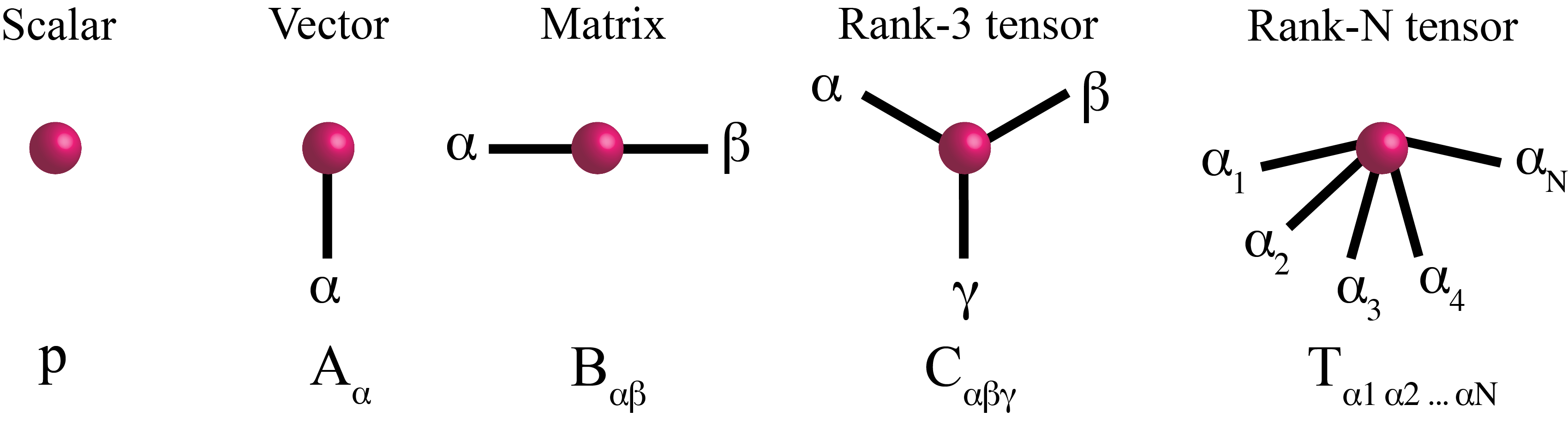
Figure 1: [Color online] Diagrammatic representation of tensors. In this notation, a rank-$n$ tensor is represented by a shape with $n$ lines such that scalers, vectors, matrices, and rank-$n$ tensors will be shapes with respectively, zero, one, two, and $n$ lines.

Tensor networks Orús and Vidal (2008); Verstraete et al. (2008) where originally developed in physics with the aim of providing efficient representations for quantum many-body wave functions. They are also the basis of well-established numerical techniques such as density matrix renormalization group (DMRG) White (1992, 1993) and time-evolving block decimation (TEBD) Vidal (2003, 2004). However, due to its high potential for efficient data representation and compression, novel applications of TNs are emerging in different branches of data science such as machine learning and optimization. In this section we show how TNs can enhance deep neural networks by providing an efficient representation of the trainable weights of classical neural networks. To this end, we first review some basic concepts on TNs in order to establish basic notation and concepts widely used in the physics’ context.

II.1 Tensor Network Basics

A tensor is a multi-dimensional array of complex numbers represented by $T_{\alpha\beta\gamma\ldots}$ in which the subscripts denote the tensor dimensions. The number of tensor dimensions further corresponds to the rank of the tensor. Tensors and tensor operations can alternatively be described by using tensor network diagrams Orús (2014) as illustrated in Fig. 1. Within this graphical representation, a rank-$n$ tensor is a shape with $n$ connected links (legs) so that a scalar, a vector, and a matrix are objects with zero, one, and two connected links, respectively. This diagrammatic notation is then generalized to rank-$n$ tensors to shapes with $n$ legs, each corresponding to a tensor index.

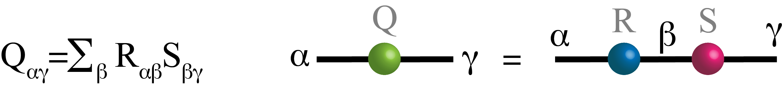
Figure 2: [Color online] Contraction of tensors, equivalent to tensor trace over their shared indices. This is represented graphically by connecting the shared links. Here, $R$ and $S$ tensors are connected along the shared leg $\beta$. This contraction operation is equivalent to matrix multiplication.

TN diagrams not only represent the tensors but also represent tensor contractions, which is the generalization of matrix multiplication to rank-$n$ tensors. For example, contraction of two rank-$2$ tensors, i.e., matrices $R_{\alpha\beta}$ and $S_{\beta\gamma}$ can be represented diagrammatically by connecting the two tensors along their shared link $\beta$, as shown in Fig. 2. This operation can further be represented mathematically as

$$Q_{\alpha\gamma}={\rm tTR}(R_{\alpha\beta}S_{\beta\gamma})=\sum_{\beta}R_{\alpha\beta}S_{\beta\gamma},$$ (1)

where the ${\rm tTR}$ is the tensor trace over shared indices (tensor legs).

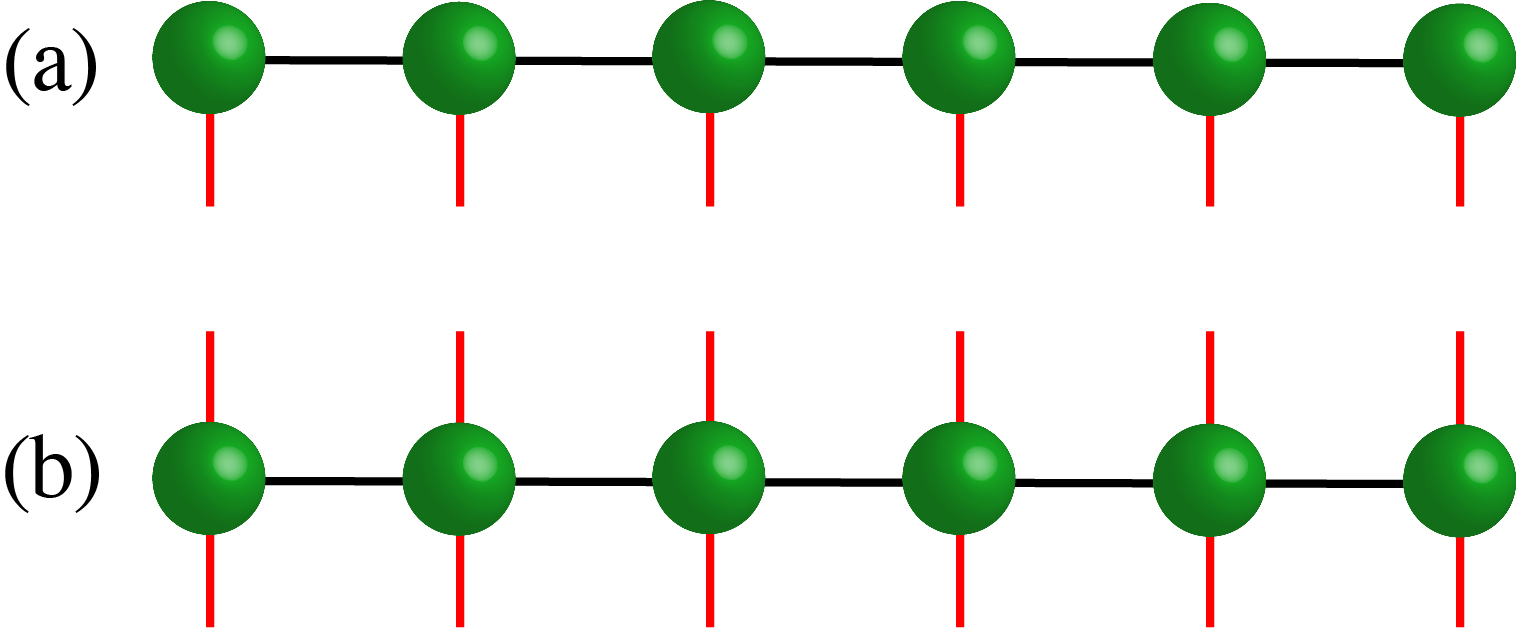
Figure 3: [Color online] Examples of well-known one dimensional TNs. (a) Matrix product states (MPS) and (b) matrix product operators (MPO). The latter will be used for representing the trainable weights of TNLayers.

Large matrices and multi-dimensional arrays with a massive number of parameters can further be represented efficiently by tensor networks. Fig. 3 shows examples of two well-known tensor networks, namely, matrix product states (MPS) (also known as a tensor trains) and matrix product operators (MPO) Verstraete et al. (2008), which are used for representing one-dimensional quantum many-body wave functions and operators. In particular, one can provide efficient MPO representations of large matrices by reducing the number of parameters in a controlled way. More specifically, a matrix can be decomposed as an MPO by applying singular value decomposition (SVD) and truncating the negligible singular values. An example of MPO factorization for a matrix $M_{p^{2}\times p^{2}}$ is shown in Fig. 4. Reshaping $M$ into a rank-$4$ tensor and applying an appropriate SVD, one can represent matrix $M$ as a 2-site MPO with tensors $L_{pp\chi}$ and $R_{\chi pp}$:

$$M=USV^{\dagger}=LR,\quad\quad L=U\sqrt{S},\quad\quad R=\sqrt{S}V^{\dagger},$$ (2)

where $U$ and $V^{\dagger}$ are unitary matrices reshaped into rank-$3$ tensors and $S$ is a diagonal matrix of singular values. For the $p^{2}\times p^{2}$ matrix $M$ there exist at most $\chi=p^{2}$ singular values. The non-zero singular values quantify the amount of entanglement (correlation) between the $L$ and $R$ MPO tensors. In a weakly correlated system, most of the singular values are close to zero and can be discarded so that only the $\chi_{t}\leq\chi$ largest singular values are kept. One can, therefore, reduce the number of parameters along the so-called virtual tensor dimensions (black link) by keeping only the most relevant degrees of freedom for the correlations between $L$ and $R$. In turn, this also implies that the interconnecting tensor dimensions which emerge in the decomposition capture the relevant degrees of freedom quantifying correlations in the tensor network.

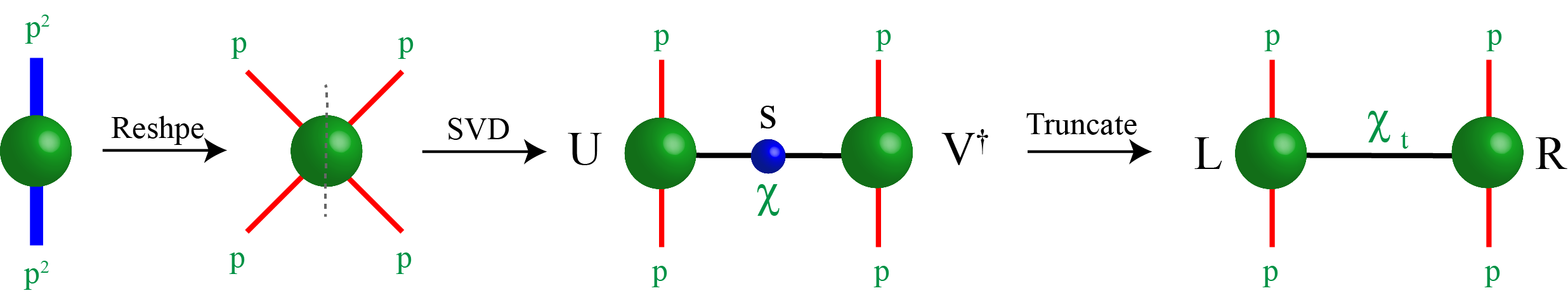
Figure 4: [Color online] Singular value decomposition of a $p^{2}\times p^{2}$ matrix $M$ into the $L$ and $R$ tensors of a 2-site MPO, see text for details.

II.2 Tensorizing Standard Neural Networks

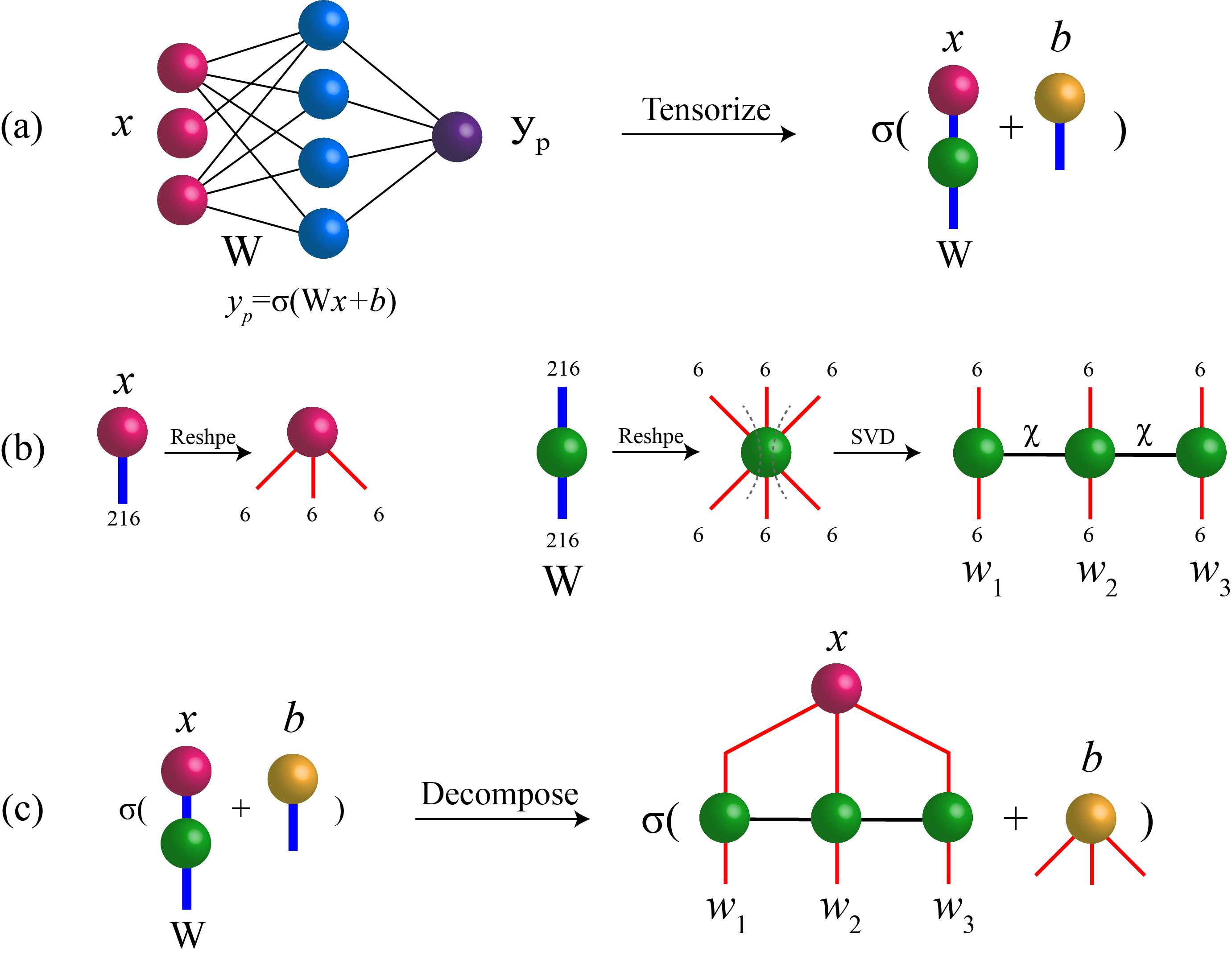
Figure 5: [Color online] Tensorizing a NN with one fully connected dense layer: (a) TN representation of the NN; (b) MPO decomposition of the weight matrix $W$; (c) The resulting tensor neural network with MPO trainable weights.

In this subsection, we show how to integrate tensor networks into standard neural networks to build a TNN. Fig. 5-(a) shows the structure of a classic NN with one fully connected Dense layer of hidden units (neurons). The network prediction, $y_{p}$, is obtained by feeding the input feature vector $x$ to the model as

$$y_{p}=\sigma(Wx+b),$$ (3)

where $W$ is the weight matrix, $b$ is some bias vector and $\sigma$ is the activation function (e.g., ReLu or Sigmoid). Training the NN amounts to finding the optimum values for the parameters of the $W$ weight matrix such that the $y_{p}$ corresponds the actual label of the data.

Depending on the size of the problem, the weight matrices can be considerably large. This introduces computational bottlenecks to the NN model from the point of view of the required memory for storing such matrices, and also due to the large training time. The problem becomes more dramatic when dealing with deep NNs with many hidden layers. Optimizing the parameters of such huge weights will reduce the accuracy and efficiency of the model. It is therefore a necessity to reduce the number of model parameters, without sacrificing accuracy. To this end, we should resort to a controllable truncation scheme such that we only discard the least important information and keep the most relevant one. An example of such clever data compression schemes based on TN and MPO decomposition has already been introduced in the previous subsection. An efficient representation of the weight matrices can therefore be obtained by replacing $W$ weights with MPOs Panagakis et al. (2021); Patel et al. (2022). Figure  5 shows how the weight matrix of a fully connected Dense layer can be replaced by its MPO form obtained from consecutive applications of SVDs to the $W$ matrix. The new tensorized layer, called TNLayer, now has several trainable weights $w_{i}$ represented by MPOs. Reshaping the feature vector $x$ to match the MPO dimensions, the network prediction $y_{p}$ is obtained by contracting the resulting tensor network as shown in 5-(c). The resulting tensorized neural network is then called a TNN.

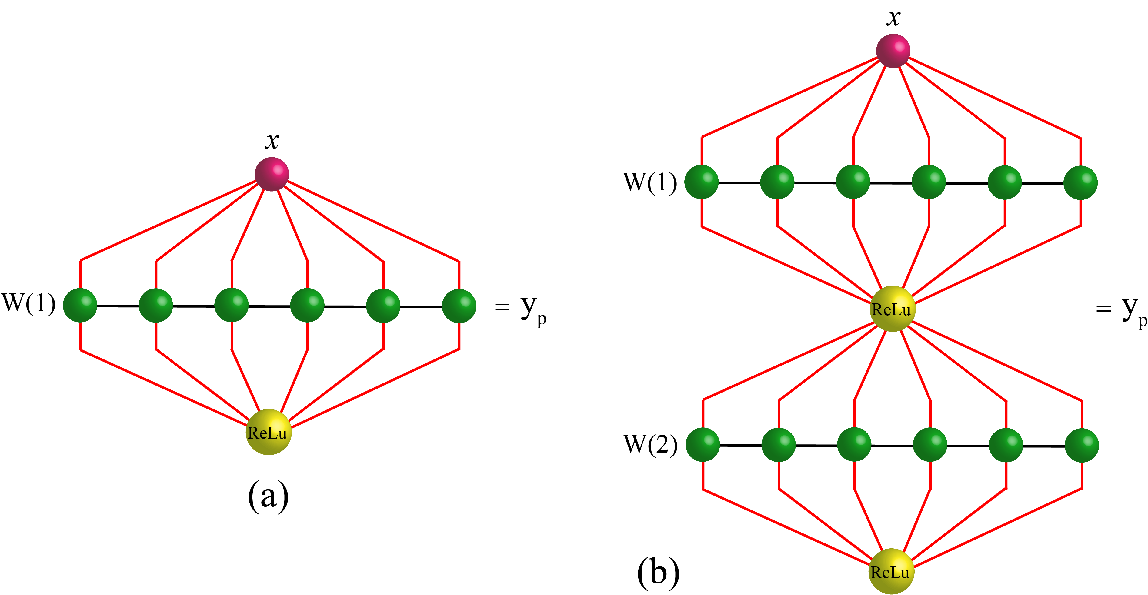
Figure 6: [Color online] Examples of fully tensorized TNNs with (a) one TNLayer and (b) with two TNLayers.

While the idea of a TNN is generic, direct tensorization can be applied to models whose feature vector $x$ is factorable to integers, so that it could match the size and number dimensions of the MPO weights. An example of a valid-size feature vector $x$ with $216$ entries is shown in Fig. 5-(b). Such a vector can be reshaped into a rank-$3$ tensor with dimension size $6$ that is can be contracted to a TNLayer with three MPO weights, each with input size $6$. The features that are not factorizable to match the MPOs in the TNLayer, can rather be transformed in the preprocessing of the machine learning task so that their new size matches the input size of the TNLayer. Otherwise, one can introduce a dummy non-trainable Dense layer with size $N_{F}\times N_{T}$ in front of the TNLayer to compensate for the size mismatch. Here $N_{F}$ is the size of the feature vector and $N_{T}$ is the input size of the contracted TNLayer.

Let us further stress that applying the activation on the TN layer is a non-linear operation and, therefore, cannot be tensorized or be applied to each MPO tensor individually. We, therefore, have to first contract the MPOs along their virtual legs to obtain a single weight matrix and then apply the activation on this matrix to obtain the network prediction, i.e.,

$$y_{p}=\sigma({\rm tTR}[x_{ijk\ldots}w_{i}w_{j}w_{k}\ldots]+b_{ijk\ldots}),$$ (4)

where the subscripts $ijk\ldots$ run over the dimensions of the feature tensor $x$. Nevertheless, we showed this operation with a single activation tensor as illustrated in Fig. 6 for examples of TNN with one and two TNLayers. In practice, one should first contract the features and MPOs, apply the activation function and then reshape the resulting tensor to match the inputs of the next layer. This process is continued until the whole network is contracted to obtain the prediction $y_{p}$.

The mandatory contraction of MPO weights enforced by the activation function can in principle be useful because one can connect the contracted TNLayer to Dense layers and design hybrid TNN models for different ML tasks. As exemplified in Secs. V and IV, we will use combinations of TNLayer and Dense layers to build different TNN models for regression and classification.

III DMRG-like Algorithm for TNNs

In the previous section we introduced the tensor neural networks and how to build them from TNLayers. In this section, we provide details about the DMRG-like training algorithm for multi-layer TNN models. Similar to generic optimizers that can be found in any ML library such as TensorFlow Abadi et al. (2015) or PyTorch Paszke et al. (2019), our DMRG-like algorithm is also of generic purpose and can be used for training different models ranging from regression to classification.

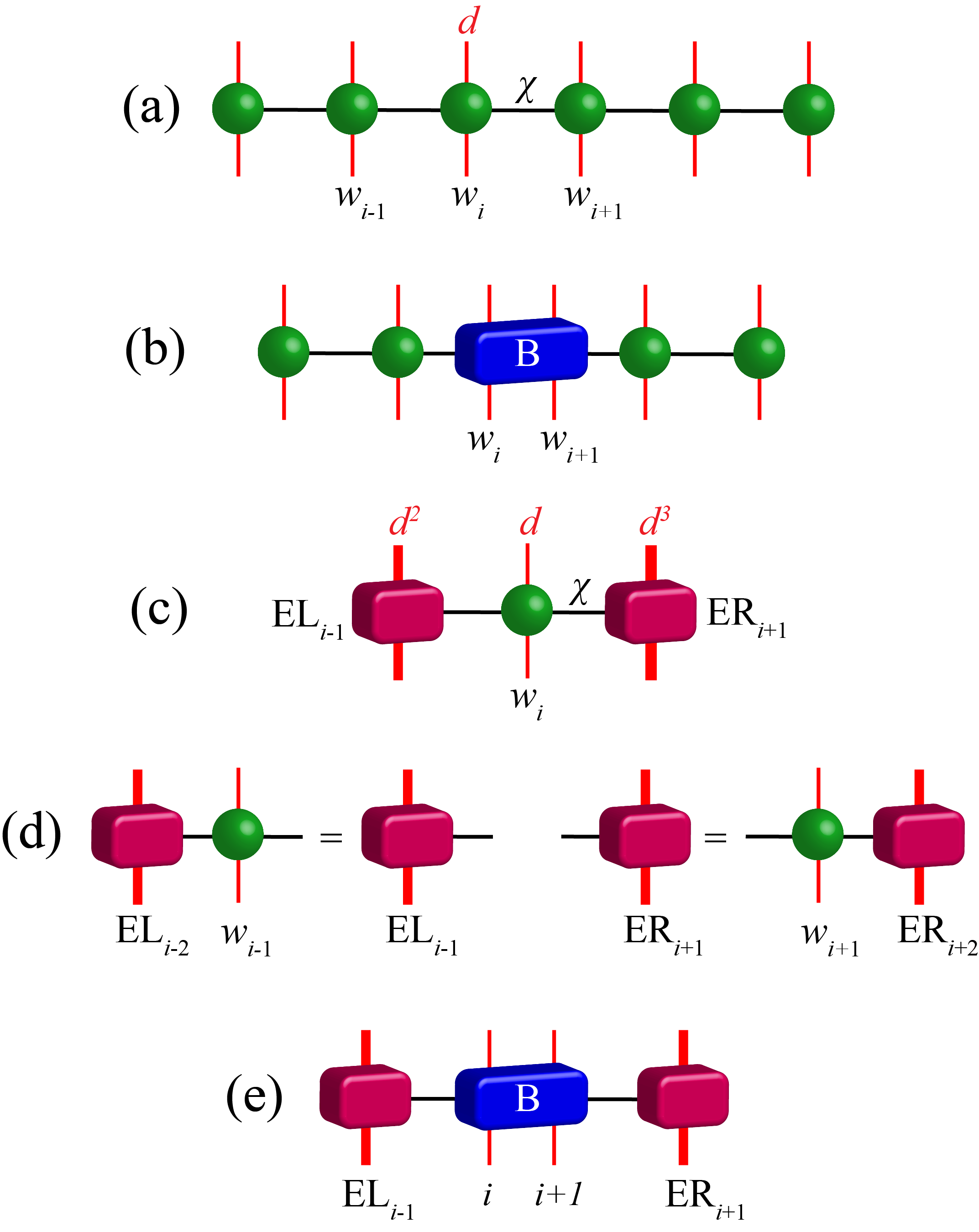
Figure 7: [Color online] Defining bond and environment tensors: (a) MPO factorized weights; (b) Bond tensor $B_{i,i+1}$ (shown in blue) which is obtained from contracting a pair of neighboring MPO tensors, $w_{i},w_{i+1}$; (c) Left and right environment tensors of each $w_{i}$ MPO tensor; (d) A single step of obtaining environment tensors; (e) Alternative representation of MPO weights in terms of bond tensor $B_{i,i+1}$ and its surrounding environment.

III.1 Local gradient-descent update

The generic idea of training a neural network is to find the optimum values for the weight matrices of the NN layers by minimizing a loss function. In a feed-forward NN, all the data or batches of it are fed to the network to calculate the $y_{p}$ in the forward path. Next, the gradients of trainable weights with respect to the loss function are calculated in the backward path, and the weights are updated accordingly with a gradient-descent (GD) step. This whole process is iterated until a convergence criterion is met. Once trained, the model is tested to predict on unseen test data. The performance of the model is further evaluated by measuring different accuracy metrics.

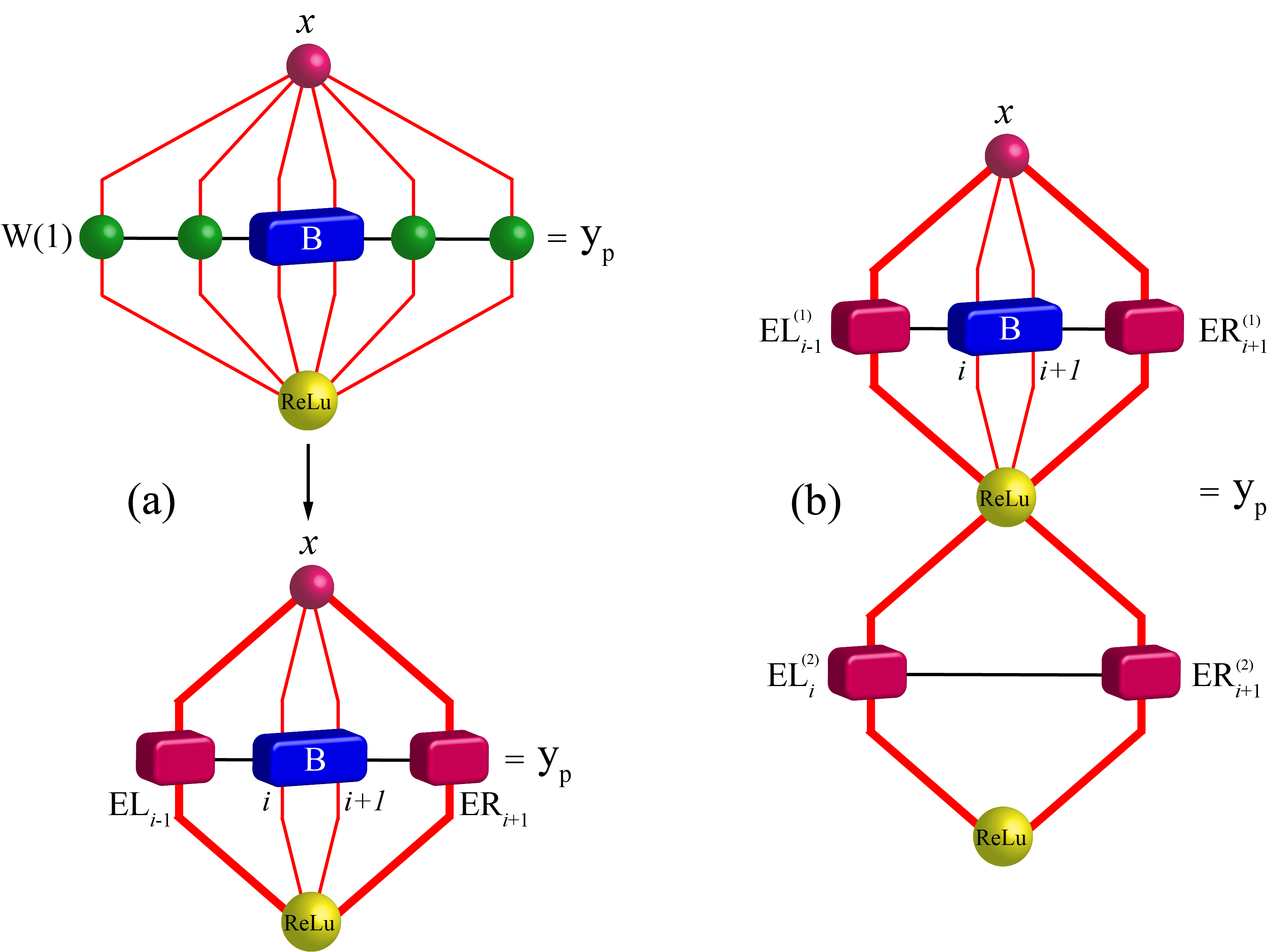
Figure 8: [Color online] Alternative representation of a TNN in terms of bond tensor $B_{i,i+1}$ and environments for (a) a TNN with one TNLayer and (b) two TNLayers.

In contrast to classic NNs with Dense layers, the TNN is composed of TNLayers that have multiple trainable MPO tensors. While a similar GD approach can be used for training the MPOs Patel et al. (2022), here we use a DMRG-like technique to update the MPO tensors by pairs, with a sweeping local gradient-descent (LGD) algorithm. However, before we present the detail of the update, the following remarks are in order: i) Given a pair of neighboring MPO tensors, $w_{i},w_{i+1}$, a bond tensor $B_{i,i+1}$ is obtained by contracting the $w_{i}$ and $w_{i+1}$ along their shared virtual dimension (see Fig. 7-(a,b)). ii) For every MPO tensor $w_{i}$, the contraction of all tensors at the right side and left side of $w_{i}$ are called environment. These are denoted by $EL_{i-1}$, $ER_{i+1}$ for the left and right environments, respectively (see Fig. 7-(c,d)). iii) For every bond tensor $B_{i,i+1}$, the TNLayer and further the overall TNN can be represented in terms of the bond tensor and its left and right environments, as shown in Fig. 7-(e) and Fig. 8. Given the fact that the TNN has to be contracted for every $B_{i,i+1}$ pair, which is required for updating the MPO weights, introducing the environment tensor can substantially reduce the computational cost of the network contraction.

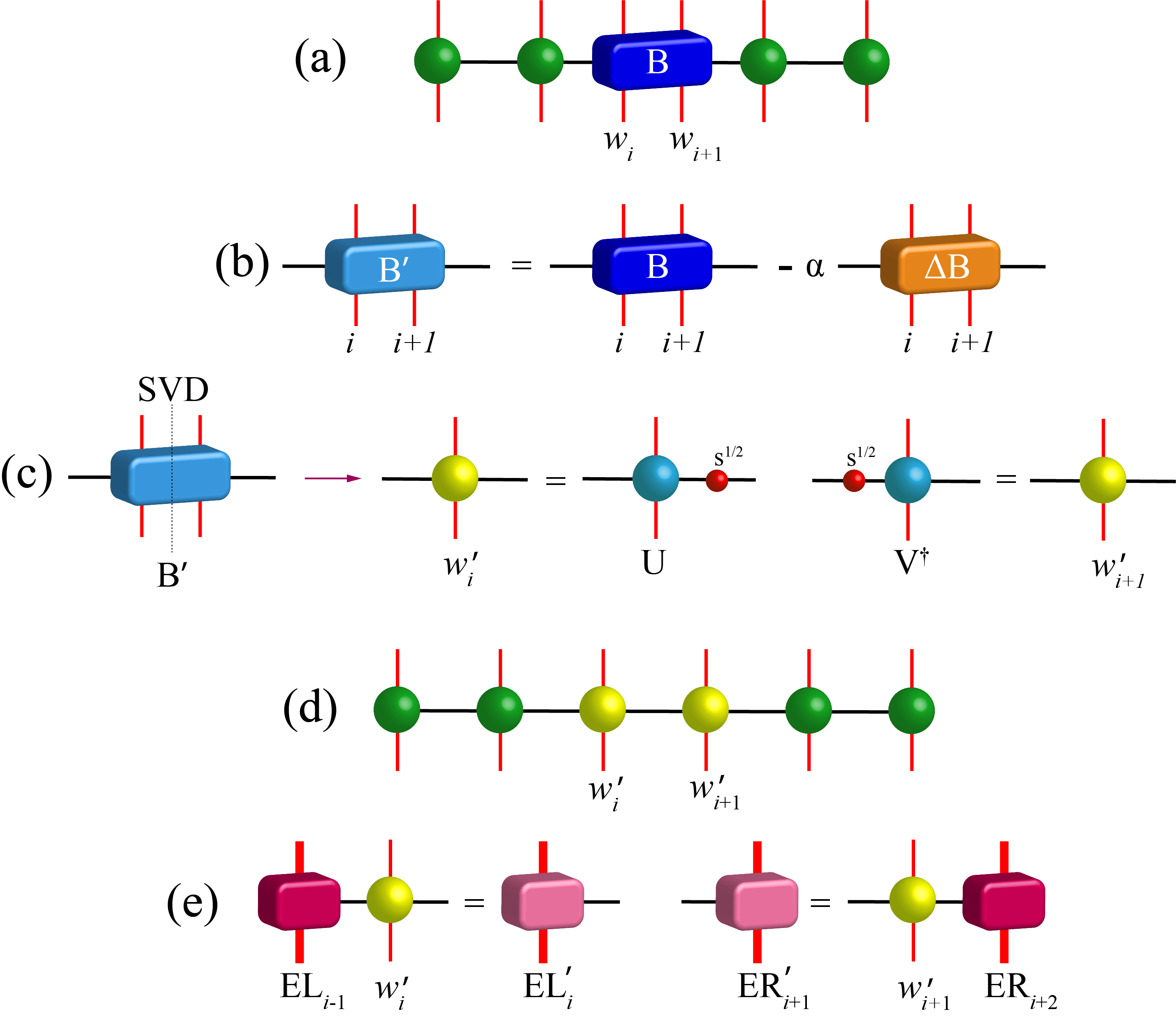
Figure 9: [Color online] Graphical representation of the DMRG-like sweeping algorithm for training TNNs: (a) MPO weights with bond tensor $B_{i,i+1}$; (b) Updating the bond tensor with LGD step; (c) Calculating the updated local weights $w^{\prime}_{i}$ and $w^{\prime}_{i+1}$ from the updated bond tensor $B^{\prime}_{i,i+1}$ by SVD and truncation; (e) Updating the left and right environments.

Having the aforementioned remarks in mind, we train the TNN by sweeping over the MPO pairs of tensors of each TNLayer as follows:

1. Do for all MPO tensor pairs $\{w_{i},w_{i+1}\}$ where $i\in[1,N_{\rm MPO}-1]$ (left to right sweep):

   1. Build the local bond tensor $B_{i,i+1}$ by contracting $w_{i}$ and $w_{i+1}$.

   2. Calculate the gradient of $B_{i,i+1}$, i.e., $\Delta B_{i,i+1}$ with respect to a loss function (see Sec. III.2, III.3).

   3. Update the bond tensor with learning rate $\alpha$: $B^{\prime}_{i,i+1}=B_{i,i+1}-\alpha\Delta B_{i,i+1}$.

   4. Split the updated bond tensor by SVD: $B^{\prime}_{i,i+1}=USV^{\dagger}$.

   5. Truncate the matrices to keep the desired number of singular values: $B^{\prime}_{i,i+1}\approx U^{\prime}S^{\prime}V^{\prime\dagger}$.

   6. Update the weights: $w^{\prime}_{i}=U^{\prime}\sqrt{S^{\prime}}$ and $w^{\prime}_{i+1}=\sqrt{S^{\prime}}V^{\prime\dagger}$.

   7. Update the left and right environment tensors: $EL^{\prime}_{i}=EL_{i-1}w^{\prime}_{i}$ and $ER^{\prime}_{i+1}=w^{\prime}_{i+1}ER_{i+2}$.

2. Sweep back from right to left and repeat the same pair update.

Details about the LGD algorithm in terms of TN diagrams are also provided in Fig. 9.

III.2 Tensor gradient for linear activations

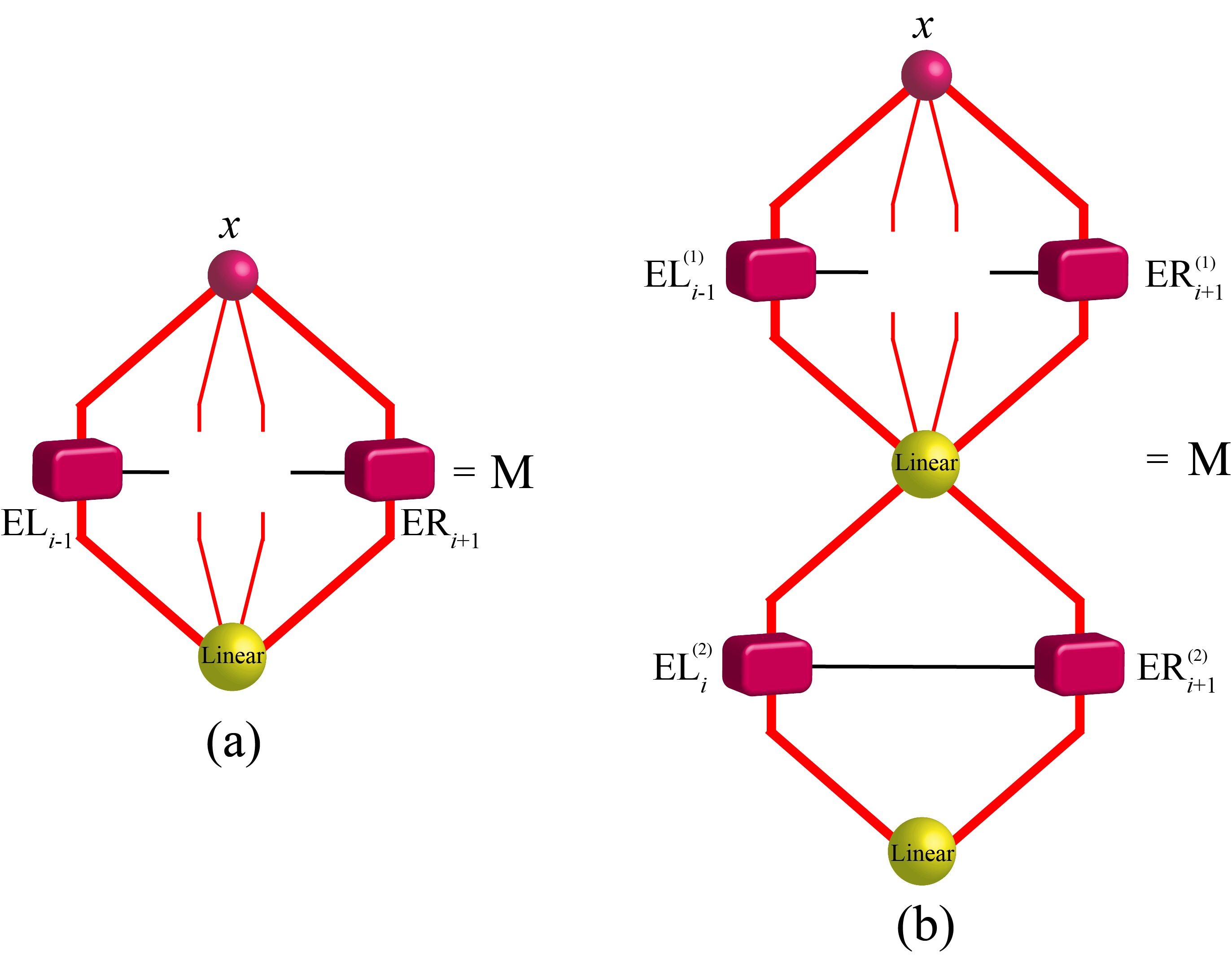
Figure 10: [Color online] The $M$ tensor required for manual calculation of the gradient $\Delta B_{i,i+1}$ for a TNN with (a) a single TNLayer, and (b) two TNLayers, and with linear activation functions.

The DMRG-like sweeping algorithm for training the TNN is a gradient-based optimization approach in which the local bond tensors, $B_{i,i+1}$, are updated towards a global minimum of a loss function by a gradient descent step with learning rate $\alpha$. Gradient of the bond tensors with respect to the loss, $\Delta B_{i,i+1}$, are therefore required for updating the weights. Given the fact that the TNN is a tensor network, gradients of the tensors in such a network with respect to a desired loss function are simply the network itself, with the corresponding tensor removed from the network. More specifically, consider a desired loss function such as the mean-squared error (MSE),

$$L_{\rm MSE}=\frac{1}{N_{s}}\sum_{j=0}^{N_{s}}(y_{p}-y_{j})^{2},$$ (5)

where $N_{s}$ is the number of training samples (input features) and $y_{j}$s are their labels. Defining $y_{p}=MB$, where $M$ is the contraction of all tensors in the TNN excluding the bond tensor $B$ (see Fig. 10), the $L_{\rm MSE}$ alternatively reads

$$L_{\rm MSE}=\frac{1}{N_{s}}\sum_{j=0}^{N_{s}}(MB-y_{j})^{2}.$$ (6)

Taking the derivative with respect to $B$, the gradient of local bond tensors is given by

$$\Delta B=-\frac{\partial L_{\rm MSE}}{\partial B}=\frac{2}{N_{s}}\sum_{n=1}^{N_{s}}(y_{j}-y_{p})M.$$ (7)

Note that while both the $M$ tensor and $y_{p}$ involve the contraction of the TNN, we do not need to do it twice. In practice, we first calculate the $M$ tensor and then we contract it to the bond tensor $B$ to obtain the $y_{p}$ prediction.

The above procedure for manual calculation of the gradient is only valid for linear activations or any other activation function that can be applied to the individual MPO weight tensors and not the contracted network. The reason is that the $M$ tensor in Fig. 10 is obtained by removing the bond tensor $B$ from the whole network after the application of the activation function. It has already been pointed out that for non-linear activations, one has to first contract the MPOs and the input from the previous layer and then apply the activation. It is obvious that the $B$ tensor can not be removed from a contracted network. Therefore, no $M$ tensor can be formed to calculate the tensor gradients manually.

Let us further remark that while the gradient in Eq. (7) and, subsequently, the LGD update (introduced in the previous subsection) are local, the DMRG-like sweep will restore the global features and correlations once iterated sufficiently.

III.3 Automatic gradient

Although the previous tensor gradient approach is suitable for TNN models fully composed of TNLayers and linear activation functions, it will not be efficient and flexible once dealing with models with hybrid architectures containing a mixture of Dense and TNLayers and nonlinear activation functions. Given the fact that our TNN is a feed-forward neural network, we can use automatic differentiation schemes and obtain the gradient of the TNN trainable weights with back-propagation (see Ref. Margossian (2019); Baydin et al. (2018) for a review on automatic differentiation and back-propagation).

While one can implement the whole process manually, implementing the TNLayer in one of the ML libraries that support the automatic differentiation is highly recommended. Here we used the TensorFlow library and one of its useful features, i.e., GradientTape Abadi et al. (2015) to record all the mathematical operations in the forward path. These include the contraction of all tensors and calculation of the network prediction, $y_{p}$, as well as the loss, ex. Eq.(5). The GradientTape uses the operation records of the forward path and calculates the gradient of all trainable vectors, matrices and tensors in the backward move. Once the gradients are obtained, every trainable weights of the TNN can be updated. The MPOs are updated as prescribed in steps (c)-(g) of the DMRG-like algorithm of Sec. III.1. The bias vectors, $b$, and the weight matrices of the Dense layers $W$ can further be updated as

$$W^{\prime}=W-\alpha\Delta W,\quad\quad b^{\prime}=b-\alpha\Delta b.$$

For hybrid TNN models composed of multiple TNLayers and Dense layers one can in principle update the weights with different strategies, i.e., layer-by-layer (LbL) or partial-all-layer (PaL). In the LbL approach, we start updating from the first layer until we reach the last output layer. The Dense layers are updated according to Eq. (III.3) and the MPO weights of TNLayers are updated by a few sweeps say $N_{\rm sweep}\leq 10$ according to the DMRG-like algorithm of Sec. III.1. On the other hand, the PaL approach targets all the layers at once. In this scheme, we consider a large $N_{\rm sweep}\geq 2000$ and update the MPO pairs $\{w^{l}_{i},w^{l}_{i+1}\}$ of all TNLayers ($l$ is the layer index), i.e, we do a multi-layer sweep. With each MPO pair update, we update the dense layers as well. This will help to reflect the local update of MPO weights in the matrix weights of the Dense layers during the sweep. The multi-layer sweep is performed until the loss converges to a certain threshold or until the $N_{\rm sweep}$ is reached.

It is also worth noting that for training the example models that we provide in the next sections, we observed that the PaL approach with large sweeps works much better from the point of view of convergence and accuracy.

Figure 11: [Color online] Binary classification of isotropic Gaussian blobs with TNN 1. The empty (filled) circles represent training (test) data.

III.4 Entanglement Entropy

In classic NN algorithms, the training convergence is checked by monitoring the loss function or some accuracy metric. The main drawback of these approaches is that they do not provide any information about the nature of the weights, the correlation among their parameters, and their expressive power. Thanks to the DMRG-like update, we have access to the singular values at every step of the sweep iterations, and this provides valuable information about the correlation (entanglement in quantum case) between MPO tensors. The individual singular values along the virtual dimensions of MPO tensors or their accumulative behavior in terms of the entropy, $S=\sum_{i}\lambda_{i}^{2}\log\lambda_{i}^{2}$, reveal the degree of correlation (entanglement) between pieces of trainable weights. While weakly correlated states are distinguished by zero or very small entanglement entropy with only a few non-zero singular values, entangled states will have non-vanishing $S$ and many non-zero singular values. Moreover, observing the behavior of entanglement entropy and singular values during the training can be used as another convergence measure, on top of the loss, which directly sheds light on the convergence of the MPO parameters.

IV TNN Classifier

After introducing the TNN and the DMRG-like sweeping algorithm, let us see the performance and accuracy of the technique for classification tasks. In what follows, we present two examples for the classification of labeled data, one for the isotropic Gaussian blobs and another for the spiral distribution, and test the TNN in action.

IV.1 Gaussian Blobs

As first example, we use the TNN to model a binary classification and train it over the random isotropic Gaussian blobs as shown with empty circles in Fig. 11. Each sample in the dataset has two position features denoted by $x_{1},x_{2}$ and a label $y=[0,1]$. The architecture of the TNN model used for the binary classification of the Gaussian blobs is detailed in Table 1. The model is composed of a TNLayer and two Dense layers. The first Dense is non-trainable and has only been added to compensate for the size mismatch between the features and the next TNLayer (see Sec. II.2). The TNLayer has six MPO trainable weights, each with input and output dimensions $d=2$, and virtual dimension $D$, and ReLu activation function. Finally the output layer is a Dense layer with Softmax activation which delivers the predicted probabilities of both labels as one-hot-encoded (OHE) vectors. The prediction $y_{p}$ can then be read form the argmax of the OHE probabilities for each sample.

Table 1: TNN architecture for binary classification of random Gaussian blobs

$N_{s}=500$, Sweep = $2000$, $\alpha=0.1$, Batch = $500$

$\mathcal{I}=\Big{\{}\{x_{1},x_{2}\},\{y\}\Big{|}\ 0\leq x_{1},x_{2}\leq 1,\ y=[0,1]\Big{\}}$

$\downarrow\ \left\{\begin{array}[]{ll}\texttt{Dense}\{\text{Units}=64,\text{trainable = }\texttt{False}\}&\\ \text{Activation: }\texttt{None }&\\ \end{array}\right.$

$\downarrow\ \left\{\begin{array}[]{ll}\texttt{TNLayer}\{\text{Units}=64,N_{\rm MPO}=6\}&\\ \text{Activation: }\texttt{ReLU }&\end{array}\right.$

$\downarrow\ \left\{\begin{array}[]{ll}\texttt{Dense}\{\text{Units}=2\}&\\ \text{Activation: }\texttt{Softmax }&\\ \end{array}\right.$

$\mathcal{O}=\text{[0,1]}$

Loss Function: BinaryCrossEntropy

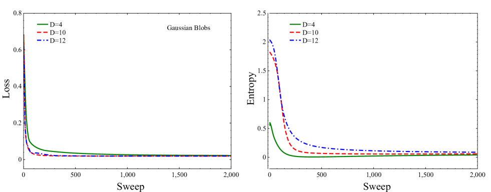
Figure 12: [Color online] (left) Training loss and (right) the $S$ entanglement entropy as a function of DMRG-like sweeps for training the TNN model 1 used for classification of Gaussian blobs.

Fig. 11 shows the distribution of the two Gaussian blobs clusters. The empty circles denote the training data and the filled circles represent the test data. We performed the training for virtual dimension $D\in[2,12]$ over $500$ training data and tested the model over $100$ unseen data. The average accuracy for classifying Gaussian blobs with the TNN model 1 is $99\%$ (see Table 1 for training hyper-parameters).

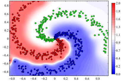
Figure 13: [Color online] Ternary classification of random spiral distribution with three classes. The red, blue and green filled circles distinguish the training data in each class. The red, white and blue shaded regions further distinguish the decision boundary obtained from training the TNN model 2.

Fig. 12 further shows the loss function and entanglement entropy as a function of the sweep iterations for different bond dimensions $D$. While both plots provide a measure for the training convergence, the $S$ suggests that the MPO weights of the TNLayer represent a weekly entangled state with a small correlation among the parameters. This is best confirmed by very small entanglement entropy (close to zero) which is a typical behavior for product states. Looking at the distribution of blobs that are categorized into two localized clusters with almost no overlap, it is expected of the MPO weights be very close to that of the product states. The TNN therefore, not only classifies the blobs but also provides expressive insight into the nature of MPO weights.

IV.2 Spiral Distribution

Table 2: TNN architecture for the classification of random spiral distributions

$N_{s}=600$, Sweep = $3000$, $\alpha=0.1$, Batch = $600$

$\mathcal{I}=\Big{\{}\{x_{1},x_{2}\},\{y\}\Big{|}\ -1\leq x_{1},x_{2}\leq 1,\ y=[0,1,2]\Big{\}}$

$\downarrow\ \left\{\begin{array}[]{ll}\texttt{Dense}\{\text{Units}=64,\text{trainable = }\texttt{False}\}&\\ \text{Activation: }\texttt{None }&\\ \end{array}\right.$

$\downarrow\ \left\{\begin{array}[]{ll}\texttt{TNLayer}\{\text{Units}=64,N_{\rm MPO}=6\}&\\ \text{Activation: }\texttt{ReLU }&\end{array}\right.$

$\downarrow\ \left\{\begin{array}[]{ll}\texttt{Dense}\{\text{Units}=3\}&\\ \text{Activation: }\texttt{Softmax }&\\ \end{array}\right.$

$\mathcal{O}=\text{[0,1,2]}$

Loss Function: BinaryCrossEntropy

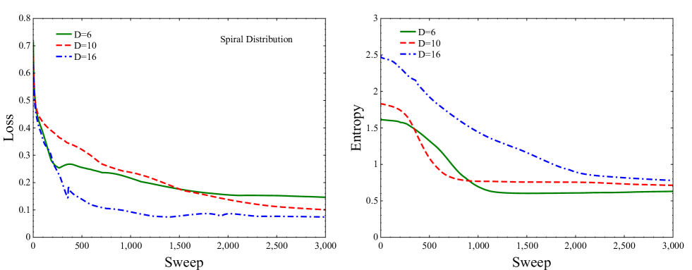
Figure 14: [Color online] (left) Training loss and (right) the $S$ entanglement entropy as a function of DMRG-like sweeps for training the TNN model 2 used for classification of spiral distibution.

For the second example, we consider a random spiral distribution with three classes as illustrated in Fig. 13. We use the TNN model described in Table 2 for the ternary classification of spiral data. The model is similar to the previous example except that now the output Dense layer has three outputs for the probabilities of each class. We trained the model over $600$ samples, $200$, for each class and obtained the decision boundary of the spiral distribution as depicted in the shaded regions with red, white, and blue colors in Fig. 13. The average accuracy of the model from different runs is $95\%$ (see Table 2 for training hyper-parameters).

The loss function and entanglement entropy during the training have also been displayed in Fig. 14 for different bond dimensions. Compared to gaussian blobs, one can clearly see that the behavior of loss and entanglement is totally different for the spiral distribution. Looking at the distribution of points in Fig. 13, the spiral dataset is expected to be more correlated and therefore, more challenging to be trained. The behavior of the loss as well as the non-vanishing entanglement entropy indeed confirms the higher degree of entanglement among the parameters of the MPOs for the spiral distribution. The $S$ for the spiral distribution is approaching $\approx 0.75$ signaling an entangled structure with more correlated parameters than that of the Gaussian blobs.

V TNN Regressor

In this section, we challenge our TNN for regression tasks. Here we present two regression examples one for fitting a line to a random linear distribution and another one for fitting to the random points around the nonlinear sine function.

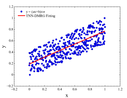
Figure 15: [Color online] Linear regression of the random data around the line $y=ax+b$ with $a=0.55$ and $b=0.20$. The red line is the fit obtained from training the TNN model 3. The predicted slope and shift of the red fitted line are $a=0.57$ and $b=0.19$.

V.1 Linear Regression

Table 3: TNN architecture for linear regression

$N_{s}=400$, Sweep = $2000$, $\alpha=0.1$, Batch = $400$

$\mathcal{I}=\Big{\{}\{x\},\{y\}\Big{|}\ 0\leq x,y\leq 1\Big{\}}$

$\downarrow\ \left\{\begin{array}[]{ll}\texttt{Dense}\{\text{Units}=64,\text{trainable = }\texttt{False}\}&\\ \text{Activation: }\texttt{None }&\\ \end{array}\right.$

$\downarrow\ \left\{\begin{array}[]{ll}\texttt{TNLayer}\{\text{Units}=64,N_{\rm MPO}=6\}&\\ \text{Activation: }\texttt{ReLU }&\end{array}\right.$

$\downarrow\ \left\{\begin{array}[]{ll}\texttt{Dense}\{\text{Units}=1\}&\\ \text{Activation: }\texttt{None }&\\ \end{array}\right.$

$\mathcal{O}=y_{p}$

Loss Function: MeanSquareError

In order to test the TNN for a linear regression problem, we generate our data by adding uniform random noise to the points out of linear function $y=ax+b$ with ($a=0.55,b=0.20$)for $0\leq x\leq 1$. The distribution of the linear random points has been depicted with blue circles in Fig. 15. In order to fit a line to the points, we designed a linear TTN model as described in Table 3. The model is composed of a single trainable TNLayer with ReLu activation and a Dense output layer with no activation. As usual, we put a non-trainable Dense layer in front of the TNLayer to compensate for the shape mismatch between the features and the TNLayer.

Training the linear TNN model for $400$ random points and $2000$ sweeps, we obtain a linear line that is perfectly fitted to the random data as shown in red in Fig. 15. Reading the slope and data shift from the predicted fitted line, we obtain $a_{p}=0.57$ and $b_{p}=0.19$ which is in good agreement with the original $a$ and $b$ parameters.

V.2 Non-linearRegression

Lastly, we challenge our TNN and DMRG-like algorithm for a non-linear regression task to predict a fit to the non-linear random points obtained by uniform noise to the $y=sinx$ function for $0\leq x\leq 2\pi$. To this end, we introduce a non-linear TNN model with three TNLayers as detailed in Table 4. Neglecting the initial dummy Dense layer, the first TNLayer has a Linear activation, and the two others have Sigmoid activation functions. Adding to this structure an output Dense layer with ReLu activation, the resulting TNN model is fully capable of capturing non-linear correlation of the input features.

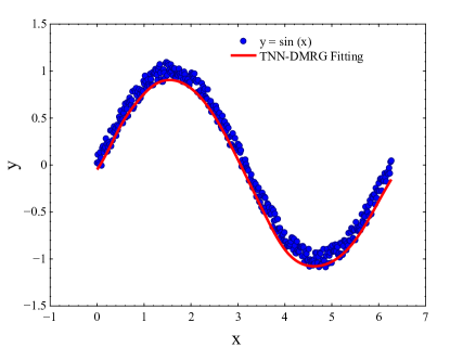
Figure 16: [Color online] Non-Linear regression of the random data introduced to the function $y=\sin x$ for $0\leq x\leq 2\pi$. The red line is the fit obtained from training the TNN model 4.

Fig. 16 shows $400$ non-linear random $sine$ shape points that have been fitted perfectly by the predicted red line from the trained TNN model. The TNN architecture of model 4 is an example of a multi-layer deep TNN which is a mixture of both Dense and TNLayers. Indeed other complicated architectures with more layers and different activations can be designed for generic ML tasks based on neural networks. The choice of these examples and hyper-parameters was to showcase the performance, accuracy, and flexibility of designing generic models with the TNN and DMRG sweeping algorithm. Indeed by changing the architecture or hyper-parameter tuning of the aforementioned models, one can improve the quality of the results. However, this was not the purpose of this study.

Table 4: TNN architecture for non-linear regression

$N_{s}=400$, Sweep = $2000$, $\alpha=0.1$, Batch = $400$

$\mathcal{I}=\Big{\{}\{x\},\{y\}\Big{|}\ 0\leq x\leq 2\pi,\ -1\leq y\leq 1\Big{\}}$

$\downarrow\ \left\{\begin{array}[]{ll}\texttt{Dense}\{\text{Units}=64,\text{trainable = }\texttt{False}\}&\\ \text{Activation: }\texttt{None }&\\ \end{array}\right.$

$\downarrow\ \left\{\begin{array}[]{ll}\texttt{TNLayer}\{\text{Units}=64,N_{\rm MPO}=6\}&\\ \text{Activation: }\texttt{Linear }&\end{array}\right.$

$\downarrow\ \left\{\begin{array}[]{ll}\texttt{TNLayer}\{\text{Units}=64,N_{\rm MPO}=6\}&\\ \text{Activation: }\texttt{Sigmoid }&\end{array}\right.$

$\downarrow\ \left\{\begin{array}[]{ll}\texttt{TNLayer}\{\text{Units}=64,N_{\rm MPO}=6\}&\\ \text{Activation: }\texttt{Sigmoid }&\end{array}\right.$

$\downarrow\ \left\{\begin{array}[]{ll}\texttt{Dense}\{\text{Units}=1\}&\\ \text{Activation: }\texttt{ReLu }&\\ \end{array}\right.$

$\mathcal{O}=y_{p}$

Loss Function: MeanSquareError

VI Conclusions and outlook

In this paper, we introduced a fully tensorized neural network model for deep learning. By replacing the trainable weight matrices of the fully connected dense layers of classic NNs with matrix product operators, we obtained tensor neural networks that are capable of modelling different machine learning tasks ranging from classification to regression. We further introduced a new entanglement-aware training algorithm based on DMRG and local gradient-descent updates for training the TNN models which act on a reduced parameter subspace obtained from the tensorization of trainable weights, and is quite fast and accurate. Our TNNs are generic-purpose, i.e., they can be used for automatizing different ML models such as regression and classification. Our implementation further allows to construct hybrid architectures with a mixture of Dense and TNLayers to build real instances of deep learning models.

In order to show the performance and accuracy of the TNNs and DMRG-like training algorithm, we considered several deep learning models for linear and non-linear regression, as well as models for the classification of labeled data. Our findings suggest that the TNNs and DMRG-like training algorithm are performing efficiently and accurately for different ML tasks. Most importantly, the DMRG-like training algorithm provides direct access to the singular values along the virtual dimensions of the trainable MPOs of TNLayers, from which a measure of entanglement (correlation) between the features and model parameters can be computed.

Our TNN and DMRG-like algorithm suggest that tensor networks are closely related to neural networks. In fact, our approach opens the door for designing new numerical techniques for obtaining neural network representations of a quantum state and is a valuable tool to study the expressive power of quantum neural states. Last but not least, The ideas developed here can further be extended to other deep learning architectures such as convolutional neural networks and their training algorithm.

VII Acknowledgements

S.S.J. acknowledges the support from Institute for Advanced Studies in Basic Sciences (IASBS), Donostia International Physics Center (DIPC) and Multiverse Computing.

References

- Zhou et al. (2017) X. Zhou, W. Gong, W. Fu, and F. Du, Proceedings - 16th IEEE/ACIS International Conference on Computer and Information Science, ICIS 2017 , 631 (2017).
- Sonoda and Kimoto (2019) J. Sonoda and T. Kimoto, Asia-Pacific Microwave Conference Proceedings, APMC 2018-November, 1298 (2019).
- Chang et al. (2018) Y. H. Chang, P. L. Chung, and H. W. Lin, Proceedings of 4th IEEE International Conference on Applied System Innovation 2018, ICASI 2018 , 66 (2018).
- Li et al. (2019) S. Li, W. Song, L. Fang, Y. Chen, P. Ghamisi, and J. A. Benediktsson, IEEE Transactions on Geoscience and Remote Sensing 57, 6690 (2019), arXiv:1910.12861 .
- Affonso et al. (2017) C. Affonso, A. L. D. Rossi, F. H. A. Vieira, and A. C. P. d. L. F. de Carvalho, Expert Systems with Applications 85, 114 (2017).
- Krizhevsky et al. (2017) A. Krizhevsky, I. Sutskever, and G. E. Hinton, Communications of the ACM 60, 84 (2017).
- Lathuiliere et al. (2020) S. Lathuiliere, P. Mesejo, X. Alameda-Pineda, and R. Horaud, IEEE Transactions on Pattern Analysis and Machine Intelligence 42, 2065 (2020), arXiv:1803.08450 .
- Ramsundar and Zadeh (2018) B. Ramsundar and R. B. Zadeh, TensorFlow for deep learning : from linear regression to reinforcement learning (O’Reilly Media, Inc., 2018).
- Tian et al. (2017) K. Tian, S. Zhou, and J. Guan, Lecture Notes in Computer Science (including subseries Lecture Notes in Artificial Intelligence and Lecture Notes in Bioinformatics) 10535 LNAI, 809 (2017).
- Min et al. (2018) E. Min, X. Guo, Q. Liu, G. Zhang, J. Cui, and J. Long, IEEE Access 6, 39501 (2018).
- Aljalbout et al. (2018) E. Aljalbout, V. Golkov, Y. Siddiqui, M. Strobel, and D. Cremers, (2018), 10.48550/arxiv.1801.07648, arXiv:1801.07648 .
- Yu et al. (2013) D. Yu, M. L. Seltzer, J. Li, J. T. Huang, and F. Seide, 1st International Conference on Learning Representations, ICLR 2013 - Conference Track Proceedings (2013), 10.48550/arxiv.1301.3605, arXiv:1301.3605 .
- Jing and Tian (2021) L. Jing and Y. Tian, IEEE Transactions on Pattern Analysis and Machine Intelligence 43, 4037 (2021), arXiv:1902.06162 .
- Dehaene and Changeux (2000) S. Dehaene and J. P. Changeux, Progress in Brain Research 126, 217 (2000).
- Hill et al. (1994) T. Hill, L. Marquez, M. O’Connor, and W. Remus, International Journal of Forecasting 10, 5 (1994).
- Bedolla et al. (2020) E. Bedolla, L. C. Padierna, and R. Castañeda-Priego, Journal of Physics: Condensed Matter 33, 053001 (2020), arXiv:2005.14228 .
- Karniadakis et al. (2021) G. E. Karniadakis, I. G. Kevrekidis, L. Lu, P. Perdikaris, S. Wang, and L. Yang, Nature Reviews Physics 2021 3:6 3, 422 (2021).
- Mehta et al. (2019) P. Mehta, M. Bukov, C. H. Wang, A. G. Day, C. Richardson, C. K. Fisher, and D. J. Schwab, Physics Reports 810, 1 (2019), arXiv:1803.08823 .
- Sharir et al. (2021) O. Sharir, A. Shashua, and G. Carleo, (2021), 10.48550/arxiv.2103.10293, arXiv:2103.10293 .
- Pescia et al. (2022a) G. Pescia, J. Han, A. Lovato, J. Lu, and G. Carleo, Physical Review Research 4, 023138 (2022a), arXiv:2112.11957 .
- Gutiérrez and Mendl (2022) I. L. Gutiérrez and C. B. Mendl, Quantum 6, 627 (2022), arXiv:1912.08831v4 .
- Pescia et al. (2022b) G. Pescia, J. Han, A. Lovato, J. Lu, and G. Carleo, Physical Review Research 4, 023138 (2022b), arXiv:2112.11957 .
- Wu et al. (2021) Y. Wu, J. Yao, P. Zhang, and H. Zhai, Physical Review Research 3, L032049 (2021), arXiv:2101.04273 .
- Carrasquilla and Melko (2017) J. Carrasquilla and R. G. Melko, Nature Physics 2017 13:5 13, 431 (2017), arXiv:1605.01735 .
- Greplova et al. (2020) E. Greplova, A. Valenti, G. Boschung, F. Schäfer, N. Lörch, and S. D. Huber, New Journal of Physics 22, 045003 (2020).
- Tanaka and Tomiya (2017) A. Tanaka and A. Tomiya, http://dx.doi.org/10.7566/JPSJ.86.063001 86 (2017), 10.7566/JPSJ.86.063001, arXiv:1609.09087 .
- Zhang et al. (2017) Y. Zhang, R. G. Melko, and E. A. Kim, Physical Review B 96, 245119 (2017).
- Orús (2014) R. R. Orús, Annals of Physics 349, 117 (2014), arXiv:1306.2164 .
- Verstraete et al. (2008) F. Verstraete, V. Murg, and J. Cirac, Advances in Physics 57, 143 (2008).
- Stoudenmire and Schwab (2016) E. M. Stoudenmire and D. J. Schwab, (2016), 10.48550/arxiv.1605.05775, arXiv:1605.05775 .
- Patel et al. (2022) R. G. Patel, C.-W. Hsing, S. S. Ahin, S. S. Jahromi, S. Palmer, S. Sharma, C. Michel, V. Porte, M. Abid, S. Aubert, P. Castellani, C.-G. Lee, S. Mugel, and R. Orús, (2022), 10.48550/arxiv.2208.02235, arXiv:2208.02235 .
- Wang et al. (2020) J. Wang, C. Roberts, G. Vidal, and S. Leichenauer, (2020), 10.48550/arxiv.2006.02516, arXiv:2006.02516 .
- Stoudenmire (2018) E. M. Stoudenmire, Quantum Science and Technology 3, 034003 (2018).
- Panagakis et al. (2021) Y. Panagakis, J. Kossaifi, G. G. Chrysos, J. Oldfield, M. A. Nicolaou, A. Anandkumar, and S. Zafeiriou, Proceedings of the IEEE 109, 863 (2021), arXiv:2107.03436 .
- Bahri et al. (2019) M. Bahri, Y. Panagakis, and S. Zafeiriou, IEEE Transactions on Pattern Analysis and Machine Intelligence 41, 2365 (2019), arXiv:1801.06432 .
- Kossaifi et al. (2017) J. Kossaifi, A. Khanna, Z. Lipton, T. Furlanello, and A. Anandkumar, IEEE Computer Society Conference on Computer Vision and Pattern Recognition Workshops 2017-July, 1940 (2017), arXiv:1706.00439 .
- Kossaifi et al. (2020) J. Kossaifi, Z. C. Lipton, A. Kolbeinsson, A. Khanna, T. Furlanello, and A. Anandkumar, Journal of Machine Learning Research 21, 1 (2020).
- Martin-Ramiro et al. (2022) P. Martin-Ramiro, U. S. de la Maza, M. Alvarez-Cascos, G. J. Alvarez, O. H. Caballer, S. S. Jahromi, R. Orus, and S. Mugel, In prepration (2022).
- White (1992) S. R. White, Physical Review Letters 69, 2863 (1992).
- White (1993) S. R. White, Physical Review B 48, 10345 (1993).
- Orús and Vidal (2008) R. Orús and G. Vidal, Physical Review B - Condensed Matter and Materials Physics 78, 155117 (2008), arXiv:0711.3960 .
- Vidal (2003) G. Vidal, Physical Review Letters 91, 147902 (2003), arXiv:0301063 [quant-ph] .
- Vidal (2004) G. Vidal, Physical Review Letters 93, 040502 (2004), arXiv:0310089 [quant-ph] .
- Abadi et al. (2015) M. Abadi, A. Agarwal, P. Barham, E. Brevdo, Z. Chen, C. Citro, G. S. Corrado, A. Davis, J. Dean, M. Devin, S. Ghemawat, I. Goodfellow, A. Harp, G. Irving, M. Isard, Y. Jia, R. Jozefowicz, L. Kaiser, M. Kudlur, J. Levenberg, D. Mané, R. Monga, S. Moore, D. Murray, C. Olah, M. Schuster, J. Shlens, B. Steiner, I. Sutskever, K. Talwar, P. Tucker, V. Vanhoucke, V. Vasudevan, F. Viégas, O. Vinyals, P. Warden, M. Wattenberg, M. Wicke, Y. Yu, and X. Zheng, “TensorFlow: Large-scale machine learning on heterogeneous systems,” (2015), software available from tensorflow.org.
- Paszke et al. (2019) A. Paszke, S. Gross, F. Massa, A. Lerer, J. Bradbury, G. Chanan, T. Killeen, Z. Lin, N. Gimelshein, L. Antiga, A. Desmaison, A. Kopf, E. Yang, Z. DeVito, M. Raison, A. Tejani, S. Chilamkurthy, B. Steiner, L. Fang, J. Bai, and S. Chintala, in Advances in Neural Information Processing Systems 32 (Curran Associates, Inc., 2019) pp. 8024–8035.
- Margossian (2019) C. C. Margossian, Wiley Interdisciplinary Reviews: Data Mining and Knowledge Discovery 9, e1305 (2019), arXiv:1811.05031 .
- Baydin et al. (2018) A. G. Baydin, B. A. Pearlmutter, A. A. Radul, and J. M. Siskind, Journal of Machine Learning Research 18, 1 (2018).