An FMM accelerated Poisson Solver for Complicated Geometries in the Plane Using Function Extension

Abstract

We describe a new, adaptive solver for the two-dimensional Poisson equation in complicated geometries. Using classical potential theory, we represent the solution as the sum of a volume potential and a double layer potential. Rather than evaluating the volume potential over the given domain, we first extend the source data to a geometrically simpler region with high order accuracy. This allows us to accelerate the evaluation of the volume potential using an efficient, geometry-unaware fast multipole-based algorithm. To impose the desired boundary condition, it remains only to solve the Laplace equation with suitably modified boundary data. This is accomplished with existing fast and accurate boundary integral methods. The novelty of our solver is the scheme used for creating the source extension, assuming it is provided on an adaptive quad-tree. For leaf boxes intersected by the boundary, we construct a universal “stencil” and require that the data be provided at the subset of those points that lie within the domain interior. This universality permits us to precompute and store an interpolation matrix which is used to extrapolate the source data to an extended set of leaf nodes with full tensor-product grids on each. We demonstrate the method’s speed, robustness and high-order convergence with several examples, including domains with piecewise smooth boundaries.

65D12, 65N50, 65N80, 65N85, 65R20

1 Introduction

We consider the problem of rapidly and accurately solving the Poisson equation

(1) $$\Delta u(\mathbf{x}) =f(\mathbf{x}),\quad\text{for }\mathbf{x}\in\Omega,$$

(2) $$u(\mathbf{x}) =g(\mathbf{x}),\quad\,\text{for }\mathbf{x}\in\partial\Omega,$$

in complicated domains in the plane. Here, $u$ is an unknown function, $f$ is a smooth source density and $g$ is the specified Dirichlet boundary data. While many fast solvers are based on direct discretization of the partial differential equation itself, recent years have witnessed substantial progress in developing solvers based on potential theory, that make use of the linearity of the problem to solve (1), (2) in two steps. One first computes a “particular solution” $v(\mathbf{x})$ that satisfies

(3) $$\Delta v(\mathbf{x})=f(\mathbf{x})\quad\text{for }\mathbf{x}\in\Omega,$$

without regard to the boundary condition, and then finds a harmonic function $w(\mathbf{x})$ that satisfies

(4) $$\Delta w(\mathbf{x}) =0\quad\text{for }\mathbf{x}\in\Omega,$$

$$w(\mathbf{x}) =g(\mathbf{x})-v(\mathbf{x}),\quad\,\text{for }\mathbf{x}\in\partial\Omega.$$

Clearly, $u(\mathbf{x})=w(\mathbf{x})+v(\mathbf{x})$ is the desired solution. Strong arguments for this approach are that (3) can be solved by an integral transform without any volumetric unknowns and that (4) can be solved using a boundary integral equation with unknowns only on the surface $\partial\Omega$ (see, for example, [2, 19, 38]).

One possible choice for $v(\mathbf{x})$ is the volume potential

(5) $$\mathcal{V}_{\Omega}[f](\mathbf{x})=\int\limits_{\Omega}G(\mathbf{x}-\mathbf{y})f(\mathbf{y})\,\mathrm{d}\mathbf{y},\quad\,\text{for }\mathbf{x}\in\Omega,$$

where $G(\mathbf{x})$ is the free-space Green’s function [14], given in the two-dimensional case by

(6) $$G(\mathbf{x},\mathbf{y})=\frac{1}{2\pi}\log\|\mathbf{x}-\mathbf{y}\|.$$

Definition 1.1.

When $\Omega$ is a square with $f(\mathbf{x})$ given at tensor product grid points on the leaf nodes of an adaptive quad-tree data structure, highly optimized fast multipole methods are available for computing volume potentials of the form (5) [12, 37]. We will refer to such methods as volume-integral fast multipole methods (VFMMs).

Remark 1.2.

VFMMs assume that $f(\mathbf{x})$ is resolved with high order accuracy by a piecewise polynomial approximation on the leaf nodes. For orders of accuracy greater than four, VFMMs typically use tensor product Chebyshev or Legendre grids on the leaf nodes for stable high order approximation. For those familiar with VFMMs, recall that (5) is computed exactly (for the piecewise polynomial approximation of the source density) in the near field and with arbitrary, user-controlled precision in the far field.

For general domains, however, VFMMs cannot be applied directly with high order accuracy, since there will be cut leaf nodes that are intersected by the boundary $\partial\Omega$ and where the data is only defined in the domain interior. This prevents simple high order polynomial approximation of $f(\mathbf{x})$ on the cut nodes, since the function is not locally smooth. In this paper, we seek to enable the application of VFMMs by first extending the function $f(\mathbf{x})$ smoothly to a function $f^{e}(\mathbf{x})$ defined on a region $E\supset\Omega$ for which a VFMM can be applied (see Fig. 4).

The combination of function extension and fast solvers is an active area of research. In [44, 45], for example, an extension of the source density $f(\mathbf{x})$ is obtained through an immersed boundary formalism. In [2], function extension is carried out using a boundary integral formulation (with harmonic extension yielding a $C^{0}$ extension, biharmonic extension yielding a $C^{1}$ extension, etc.). Once the extended function has been obtained, the fully adaptive solver of [2] computes the extended volume integral using the VFMM algorithm of [12, 23]. Another approach is Fourier continuation. One such scheme is described in [9], where the source density is extended normal to the boundary, through projection onto a basis that vanishes in the vicinity of the boundary. For a good discussion of Fourier-based extension, see [7]. In the active penalty method [42], an extension is created by matching boundary data and normal derivatives up to order $k$ in terms of a carefully crafted set of basis functions which gives an extension with global regularity $C^{k}$.

Function extension is not the only way in which the computation of volume potentials can be accelerated using VFMMs. One alternative is to modify the VFMM algorithm to treat the cut leaf nodes via more elaborate approximation and quadrature tools that depend on the precise intersection of $\partial\Omega$ with the leaf node (see [1] and the references therein). Another alternative is the recently developed technique of function intension [43], where the source density is coverd by regular tensor product leaf nodes on an adaptive quad-tree in the interior of $\Omega$, blended with a conforming mesh in the neighborhood of the boundary. This permits the use of a VFMM for the interior degrees of freedom, but needs to be coupled to an auxiliary fast Poisson solver on a tubular neighborhood of the boundary.

In this paper, we describe our new function extension algorithm in detail, using the Dirichlet problem for the Poisson equation as our model. The method is fully adaptive in the interior of the domain, high-order accurate, robust, and fast. The main novelty lies in creating a universal, level-independent, oversampled interpolation matrix, recruiting sufficient data from the neighbors of cut leaf nodes, and defining the range of the extension based on the local mesh size of the adaptive discretization. Our method is similar to the partition of unity extension scheme (PUX) developed in [21] for uniform grids. In the present scheme, however, blending and partitions of unity are avoided. Instead, the extension for each cut leaf node is entirely local, based only on data from the square itself or its nearest neighbors. Moreover, there is no need to truncate the function smoothly to zero; we simply extend it to cover a domain $E\supset\Omega$ which is discretized as a collection of leaf nodes beyond which $f(\mathbf{x})$ is identically zero (Fig. 4). (In PUX, the data is represented on a uniform grid, rather than a quad-tree, extended smoothly to zero, with a global interpolation framework based on the fast Fourier transform.) Rather than (5), the VFMM then computes the volume potential

(7) $$v(\mathbf{x})=\mathcal{V}_{E}[f^{e}](\mathbf{x})=\int_{E}G(\mathbf{x-y})f^{e}(\mathbf{y})\,d{\mathbf{y}}$$

where $f^{e}$ is the smooth extension of $f$.

An important feature of our method is that it is agnostic to the smoothness of the boundary. It simply assumes that the adaptive quad-tree has resolved the source data well enough, and that the user can identify points as being either inside or outside the domain. We will demonstrate that with an eighth order accurate VFMM, we obtain an eighth order accurate scheme for the full problem, even on piecewise smooth domains. We will also show that the overall approach is compatible with other extension schemes, including one-dimensional extensions along lines, using either the rational function approximation of [15] or the diffeomorphism-based method of [11]. For a review of

There are, of course, drawbacks to extensions schemes - the major ones being caustics and ill-conditioning. The former arise when a domain boundary curves back on itself, so that two exterior normals intersect close to the domain. This can be overcome by ensuring that the length scale of leaf nodes in the quad-tree near such points must be commensurate with the distance to the nearest such intersection. The difficulty is that this constraint could result in excessive refinement, even though the geometry and the data may be simple to resolve. Ill-conditioning is an inherit concern with function extension, since it is an extrapolation process. This effect is mitigated by the fact that, as the quad-tree is refined, the data becomes locally smoother on the scale of the leaf node and the extension problem becomes simpler as well. A detailed analysis of the conditioning of the process remains to be carried out, but experiments indicate that our method performs well without excessive resolution. The algorithm requires that data be provided at auxiliary nodes close to the boundary, but this is to be expected in a high-order formulation, and the node locations are specified as soon as the quad-tree is created, so can be considered part of the discretization process.

This paper is organized as follows. In Section 2, we review the needed elements of classical potential theory for the Poisson equation, and in Section 3, we discuss function extension with Gaussians. In Section 4, we present the data structures used to discretize the right-hand side $f(\mathbf{x})$ and create its extension. Layer potentials are discussed in more detail in Section 5 and the performance of the algorithm is illustrated in Section 6, along with a discussion of some implementation details. In Section 7, we discuss extensions of the present scheme and consider avenues for future improvement.

2 Mathematical preliminaries

Let $D$ be an open, bounded subset of $\mathbb{R}^{2}$, which is either simply or multiply connected. For a point $\mathbf{x}$ in $\mathbb{R}^{2}$, we will denote its Cartesian components by $(x_{1},x_{2})$ and its Euclidean norm by $\|\mathbf{x}\|$. For $\mathbf{x},\mathbf{y}$ in $\mathbb{R}^{2}$, their inner product will be denoted by $\mathbf{x}\cdot\mathbf{y}$. Unless otherwise stated, we assume that the domain has a boundary $\partial\Omega$ which is at least twice continuously differentiable. In the case of an interior problem, $\Omega=D$ and the problem is fully specified. In the case of an exterior problem, $\Omega=\mathbb{R}^{2}\setminus\bar{D}$, in which case we must also specify a condition at infinity for the problem to be well-posed. That is, we must specify a constant $A$ such that

(8) $$u(\mathbf{x})\rightarrow A\log(\|\mathbf{x}\|)$$

as $\|\mathbf{x}\|\rightarrow\infty$ [16, 30]. Bounded solutions correspond to setting $A=0$.

For simplicity, let us begin with the interior problem in a simply-connected domain. By standard potential theory [16, 26, 30], an explicit representation of the solution $u$ can be formulated as

(9) $$u(\mathbf{x})=\mathcal{V}_{E}[f^{e}](\mathbf{x})+\mathcal{D}[\sigma](\mathbf{x}),\quad\,\text{for }\mathbf{x}\in\Omega,$$

where the volume potential $\mathcal{V}_{E}[f^{e}](\mathbf{x})$ is defined in (7), so long as $E\supset\Omega$ and $f^{e}=f$ within $\Omega$. Here,

(10) $$\mathcal{D}[\sigma](\mathbf{x})=\int\limits_{\partial\Omega}\frac{\partial G(\mathbf{x}-\mathbf{y})}{\partial\boldsymbol{\nu}(\mathbf{y})}\sigma(\mathbf{y})\,\mathrm{d}s,\quad\,\text{for }\mathbf{x}\in\Omega,$$

is the double layer potential, with unknown layer density $\sigma\colon\partial\Omega\rightarrow\mathbb{R}$, $\boldsymbol{\nu}(\mathbf{y})$ denotes the unit normal at the point $\mathbf{y}\in\partial\Omega$, and $\frac{\partial G(\mathbf{x}-\mathbf{y})}{\partial\boldsymbol{\nu}(\mathbf{y})}$ denotes the normal derivative of the Green’s function (6). It is straightforward to see that $\mathcal{D}[\sigma](\mathbf{x})$ is harmonic and that the kernel of $\mathcal{D}[\sigma]$ in Eq. 10 is

(11) $$\frac{\partial G(\mathbf{x}-\mathbf{y})}{\partial\boldsymbol{\nu}(\mathbf{y})}=\frac{1}{2\pi}\frac{(\mathbf{x}-\mathbf{y})\cdot\boldsymbol{\nu}(\mathbf{y})}{\|\mathbf{x}-\mathbf{y}\|^{2}}.$$

Note that the limiting value of Eq. 11, as $\mathbf{x}$ approaches $\mathbf{y}$ along the boundary, is $-\tfrac{1}{2\pi}\kappa(\mathbf{y})$, where $\kappa(\mathbf{y})$ is the curvature at $\mathbf{y}$. Thus, assuming the boundary is at least twice differentiable, the kernel is a continuous function. For a $C^{k+2}$ boundary, the kernel is $C^{k}$.

In order to satisfy the desired Dirichlet boundary conditions, Eq. 2, we seek a layer density $\sigma$ such that $\mathcal{D}[\sigma](\mathbf{x})=g(\mathbf{x})-\mathcal{V}_{E}[f^{e}](\mathbf{x})$ for $\mathbf{x}$ on $\partial\Omega$. This is achieved by taking the limit of (9) as $\mathbf{x}$ approaches the boundary from the interior and applying standard jump conditions [32], yielding the integral equation

(12) $$(-\tfrac{1}{2}+\mathcal{D})[\sigma](\mathbf{x})=g(\mathbf{x})-\mathcal{V}_{E}[f^{e}](\mathbf{x}),\quad\text{for }\mathbf{x}\in\partial\Omega.$$

Equation 12 is a Fredholm integral equation of the second kind for $\sigma$, since $\mathcal{D}[\sigma]$ is a compact operator with a continuous kernel on a $C^{2}$ boundary (as noted above). It follows by the Fredholm alternative that Eq. 12 has a unique solution [3]. Once $\sigma$ has been obtained, we have a complete solution to the full problem.

Remark 2.1.

For Neumann boundary value problems, where (2) is replaced by

(13) $$\frac{\partial u}{\partial\boldsymbol{\nu}}(\mathbf{x})=g(\mathbf{x}),\quad\,\text{for }\mathbf{x}\in\partial\Omega,$$

the approach is essentially the same, except that the homogeneous solution is expressed as a single layer potential

(14) $$\mathcal{S}[\sigma](\mathbf{x})=\int\limits_{\partial\Omega}G(\mathbf{x}-\mathbf{y})\,\sigma(\mathbf{y})\,\mathrm{d}s,\quad\,\text{for }\mathbf{x}\in\Omega.$$

Imposing (13) leads to a second kind Fredholm equation, ensuring a unique solution (up to an arbitrary constant) so long as $\int_{\partial\Omega}g(\mathbf{x})\,ds=0$.

For the exterior Dirichlet problem in $\Omega=\mathbb{R}^{2}\setminus\bar{D}$, we first compute a particular solution of the form (7), where the extension is now into $D$. The exterior harmonic correction is then represented in the form

(15) $$u^{H}(\mathbf{x})=\mathcal{D})[\sigma](\mathbf{x})+\frac{1}{2\pi}\,\int\limits_{\partial\Omega}\sigma(\mathbf{y})\,\mathrm{d}s\,+\,\alpha\,\log\|\mathbf{x}-\mathbf{x}_{D}\|,$$

where $\mathbf{x}_{D}$ lies in $D$. Letting $Q=\frac{1}{2\pi}\iint_{E}f^{e}(\mathbf{y})\,\mathrm{d}\mathbf{y}$, we impose the additional constraint

(16) $$\alpha=A-Q$$

to ensure the user-specified radiation condition (8). For a discussion of uniqueness of the resulting integral equation, see [22, 39].

2.1 Multiply-connected domains

We now consider the interior problem for a multiply connected domain, whose boundary consists of $(N_{\Omega}+1)$ closed curves. The outer boundary curve is denoted $\partial\Omega_{0}$, and the interior boundary curves are denoted by $\partial\Omega_{1},\ldots,\partial\Omega_{N_{\Omega}}$ (see Fig. 1). In this setting, it turns out that there are $N_{\Omega}$ nontrivial homogeneous solutions to the boundary integral equation Eq. 12 [16]. In order to ensure uniqueness, we proceed as in [22], and write the full solution to the Poisson equation in the form

(17) $$u(\mathbf{x})=\mathcal{V}_{E}[f^{e}](\mathbf{x})+\mathcal{D}[\sigma](\mathbf{x})+\sum\limits_{k=1}^{N_{\Omega}}A_{k}\log\|\mathbf{x}-\mathbf{s}_{k}\|,\quad\,\text{for }\mathbf{x}\in\Omega,$$

where $\mathbf{s}_{k}$ is a point inside the interior curve $\partial\Omega_{k}$ and $\{A_{k}\}_{k=1}^{N_{\Omega}}$ are unknown constants, with the additional constraints

(18) $$\int\limits_{\partial\Omega_{k}}\sigma(\mathbf{y})\,\mathrm{d}\mathbf{y}=0,\quad\,k=1,\ldots,N_{\Omega}.$$

Imposing the Dirichlet boundary conditions together with Eq. 18 leads to an invertible Fredholm equation of the second kind for the unknowns $\sigma$ and $\{A_{k}\}_{k=1}^{N_{\Omega}}$.

Finally, we consider the Dirichlet problem posed in the region exterior to a collection of $N_{\Omega}$ closed curves $\partial\Omega_{1},\ldots,\partial\Omega_{N_{\Omega}}$. It is shown in [22], that the representation

(19) $$u^{H}(\mathbf{x})=\mathcal{D}[\sigma](\mathbf{x})+\frac{1}{2\pi}\int\limits_{\partial\Omega}\sigma(\mathbf{x})\,\mathrm{d}\mathbf{x}\ +\sum\limits_{k=1}^{N_{\Omega}}A_{k}\log\|\mathbf{x}-\mathbf{s}_{k}\|,\quad\,\text{for }\mathbf{x}\in\Omega,$$

together with the constraints

(20) $$\int\limits_{\partial\Omega_{k}}\sigma(\mathbf{y})\,\mathrm{d}\mathbf{y}=0,\quad\,k=1,\ldots,N_{\Omega}-1\quad,\quad\sum_{k=1}^{N_{\Omega}}A_{k}=A,$$

leads to a well-conditioned Fredholm equation of the second kind for $\sigma$ and $\{A_{k}\}_{k=1}^{N_{\Omega}}$.

Remark 2.2.

We will also consider domains with piecewise smooth boundaries. For such geometries, the double layer operator is no longer compact, but there is an extensive literature on the invertibility of the corresponding integral equation (see [48, 10]) and the design of high order methods for its solution (see, for example, [8, 27, 29]).

Figure 1: Left: An example geometry for the interior problem on an $(N_{\Omega}+1)$ply connected domain. Right: An example geometry for the exterior problem on an $(N_{\Omega})$ply connected domain

3 Function extension

We turn now to the problem of extending the function $f(\mathbf{x})$ defined on $\Omega$ to a function $f^{e}(\mathbf{x})\in C^{q}(E)$ on a region $E\supset\Omega$ for which a VFMM can be applied. Our scheme is based on local extrapolation using a basis of Gaussians, with a precomputed interpolation matrix that can be obtained using the RBF-QR algorithm[17], discussed briefly below. This approach is similar to local extension in the PUX algorithm [21]. However, the scheme presented here has fewer parameters and requires neither a smooth taper to zero nor a blending of multiple local extensions through a partition of unity.

3.1 Interpolation in a Gaussian basis

Consider the approximation

(21) $$I_{f}(\mathbf{x})=\sum\limits_{i=1}^{N_{\mathcal{G}}}\lambda_{i}\phi_{i}(\mathbf{x}),\quad\mathbf{x}\in\bar{S},$$

of a function $f\in C^{q}(\bar{S})$, with $q\geq 0$ on the bounded domain $\bar{S}\subset\mathbb{R}^{d}$ for $d=1,2,3$, with weights $\{\lambda_{i}\}_{i=1}^{N_{\mathcal{G}}}$. The basis consists of Gaussians $\phi_{i}(\mathbf{x})=e^{-\varepsilon^{2}\|\mathbf{x}-\mathbf{c}_{i}\|^{2}}$ centered at a set of distinct points ${\mathcal{G}}=\{\mathbf{c}_{i}\}_{i=1}^{N_{\mathcal{G}}}$ in $\bar{S}$. We will refer to $\varepsilon$ as a shape parameter, with smaller values corresponding to flatter basis functions. Clearly, $I_{f}\in C^{\infty}(\bar{S})\subset C^{q}(\bar{S})$.

Let ${{\mathcal{P}}}=\{{{\mathbf{p}}}_{i}\}^{N_{{\mathcal{P}}}}_{i=1}$ be a set of $N_{\mathcal{P}}$ distinct points in $\bar{S}$ and suppose that we wish to approximate the function values at ${{{\mathcal{P}}}}$ using the representation (21). The weights $\Lambda=(\lambda_{j})\in\mathbb{R}^{N_{\mathcal{G}}}$ can be obtained by solving the linear system

(22) $${\mathbf{\Phi}}_{{\mathcal{P}},\mathcal{G}}\Lambda={\bf f}_{\mathcal{P}},$$

where ${\mathbf{\Phi}}_{{\mathcal{P}},\mathcal{G}}\in\mathbb{R}^{N_{{\mathcal{P}}}\times N_{\mathcal{G}}}$ with ${\mathbf{\Phi}}_{{\mathcal{P}},\mathcal{G}}[i,j]=(\phi_{j}({{\mathbf{p}}}_{i}))$ and ${\bf f}_{\mathcal{P}}=(f({{\mathbf{p}}}_{1}),\dots,f({{\mathbf{p}}}_{N_{\mathcal{G}}}))$. If $N_{{\mathcal{P}}}>N_{\mathcal{G}}$, then we solve for $\Lambda$ in a least squares sense.

Approximation via a sum of Gaussians is a particular case of radial basis function approximation [34, 17, 41], and we do not seek to review the literature here, except to note that high order accuracy can be achieved by a careful interplay of the shape parameter $\varepsilon$ and $N_{\mathcal{G}}$. This requires carefully letting $\varepsilon\rightarrow 0$ while increasing $N_{\mathcal{G}}$ [34, 17, 41]. If $\varepsilon$ were fixed, convergence would stagnate with $N_{\mathcal{G}}$. On the other hand, for a fixed $N_{\mathcal{G}}$, the linear system (22) becomes increasingly ill-conditioned as $\varepsilon\rightarrow 0$, resulting in oscillatory weights $\Lambda$. Following [35], it turns out that one can construct a well-conditioned interpolation problem for $\varepsilon\approx 10^{-5}$ on the unit box, achieving high order convergence. This involves reformulating Eq. 22 to avoid explicit use of the weights $\Lambda$. For this, let

$${\bf f}_{\mathcal{G}}=(f(\mathbf{c}_{1}),\dots,f(\mathbf{c}_{N_{\mathcal{G}}}))\in\mathbb{R}^{N_{\mathcal{G}}}.$$

If we formally collocate Eq. 21 at $\mathcal{G}$, then $\Lambda=\Phi_{\mathcal{G},\mathcal{G}}^{-1}{\bf f}_{\mathcal{G}}$ and we may rewrite Eq. 22 in the form

(23) $${\mathbf{A}}_{{\mathcal{P}},\mathcal{G}}{\bf f}_{\mathcal{G}}={\bf f}_{\mathcal{P}},$$

where ${\mathbf{A}}_{{\mathcal{P}},\mathcal{G}}={\mathbf{\Phi}}_{{\mathcal{P}},\mathcal{G}}\Phi_{\mathcal{G},\mathcal{G}}^{-1}$ to directly obtain the desired values ${\bf f}_{\mathcal{G}}$. While this formulation avoids $\Lambda$, it remains to address the ill-conditioning of $\Phi_{\mathcal{G},\mathcal{G}}$. It turns out that stable, accurate solutions can be obtained using the RBF-QR method [17]. The essential idea is to expand each Gaussian in an intermediate (well-conditioned) basis consisting of a combination of powers, Chebyshev polynomials, and trigonometric functions. Leaving out the details, the total cost of RBF-QR is of the order $\mathcal{O}(N_{{\mathcal{P}}}N_{\mathcal{G}}M^{2})$, where $M>N_{\mathcal{G}}$ is the number of functions used in the intermediate basis. This cost would be prohibitive if carried out at every cut leaf node in our adaptive discretization. However, if the sets ${\mathcal{P}}$ and $\mathcal{G}$ are universal, then ${\mathbf{A}}$ can be precomputed and stored. In that case, the cost of solving the least squares problem (23) is of the order $\mathcal{O}(N_{{\mathcal{P}}}N_{\mathcal{G}}^{2}+N_{\mathcal{G}}^{3})$. In the next section, we describe how to construct such a univeral matrix.

3.2 Extension from cut leaf nodes

Let $S$ be a square of sidelength $L$ which is cut by the boundary $\Gamma$ of our domain $\Omega$, and let $\mathcal{X}_{S}$ be the $K\times K$ tensor product Chebyshev grid scaled to $S$. We define the extension square $\bar{S}$ to be a square of sidelength $3L$, with the same center as $S$ (see Fig. 2). The $\bar{K}\times\bar{K}$ tensor product Chebyshev grid scaled to $\bar{S}$ is denoted by $\mathcal{X}_{\bar{S}}$.

On that square, we also impose a uniform triangulation, and constructing a Delaunay triangulation. The vertices of that triangulation are chosen as the Gaussian support nodes $\mathcal{G}$. The details of the construction are not so important - just that the number be slightly greater than $O(K^{2})$ and that they be approximately uniformly distributed in the square. Let ${\mathcal{P}}=\mathcal{X}_{S}\cup\mathcal{X}_{\bar{S}}\cup\mathcal{G}$. For any of these point sets, we let the superscript ${\cal I}$ refer to the subset that lies in the interior of $\Omega$ and we let the superscript ${\cal E}$ refer to the subset that lies in the exterior of $\Omega$. Thus, ${\mathcal{P}}^{\cal I}$ denotes the subset of ${{\mathcal{P}}}$ that lies in the interior of $\Omega$, and $\mathcal{X}_{\bar{S}}^{\cal E}$ denotes the subset of ${\mathcal{X}_{\bar{S}}}$ that lies in the exterior of $\Omega$. The full matrix ${\mathbf{A}}_{{\mathcal{P}},\mathcal{G}}$ is universal and can clearly be computed and stored. Extracting the rows corresponding to interior points results in the matrix ${\mathbf{A}}_{{{\mathcal{P}}}^{\cal I},\mathcal{G}}$, while extracting the rows corresponding to ${\mathcal{X}_{\bar{S}}^{\cal E}}$ results in ${\mathbf{A}}_{\mathcal{X}_{\bar{S}}^{\cal E},\mathcal{G}}$. Assuming that the function $f$ is known at ${{\mathcal{P}}}^{i}$, we can obtain its extension $f_{\mathcal{X}_{\bar{S}}^{\cal E}}$ as

$$f_{\mathcal{X}_{\bar{S}}^{\cal E}}={\mathbf{A}}_{\mathcal{X}_{\bar{S}}^{\cal E},\mathcal{G}}{\mathbf{A}}_{{{\mathcal{P}}}^{\cal I},\mathcal{G}}^{\dagger}f_{{{\mathcal{P}}}^{\cal I}}.$$

where ${\mathbf{A}}_{{{\mathcal{P}}}^{\cal I},\mathcal{G}}^{\dagger}$ denotes the pseudo-inverse of ${\mathbf{A}}_{{{\mathcal{P}}}^{\cal I},\mathcal{G}}$. This yields the missing values to extend $f$ to a full tensor product Chebyshev grid $\mathcal{X}_{\bar{S}}$ on the extension square ${\bar{S}}$. From this, we can easily compute $f^{e}$ at any point in $\bar{S}$ by interpolation.

Figure 2: A cut cell $S$ of interest (the central square) and its 8 near neighbors at the same scale. Their union defines the extension square $\bar{S}$. In this case, suppose that the region below the curve (light blue) corresponds to the domain interior and the region above the curve (light purple) corresponds to the exterior. The marked points with a blue, circular shape in $S$ are the scaled Chebyshev nodes on $S$. The marked points with a black, diamond shape are the scaled Chebyshev nodes on $\bar{S}$. The marked points with a red, square shape are the support nodes for the Gaussian basis functions. The points in each of these sets that lie in the domain interior are indicated with filled markers. The points in these sets that lie in the domain exterior are indicated with unfilled markers. In our extension algorithm, we construct a least-squares interpolant at the interior points and use it to obtain values at the Chebyshev nodes on $\bar{S}$.

4 Discretization, data structures, and the volume potential

We turn now to the task of function extension from a complicated domain $\Omega$ to a larger domain $E$ for which the VFMM can be applied with high order accuracy. We assume, without loss of generality, that $\Omega$ is contained in the unit square $D$ centered at the origin, and that the support $E$ of $f^{e}$ (which is only slightly larger than $\Omega$) is contained in $D$ as well. We assume that the boundary $\partial\Omega$ is provided in the form

$$\partial\Omega=\bigcup\limits_{i=1}^{N_{\Gamma}}\Gamma_{i},$$

where we refer to the disjoint segments $\{\Gamma_{i}\}_{i=1}^{N_{\Gamma}}$ as panels, and each panel is defined by a parametrization

$$\Gamma_{i}=\{\boldsymbol{\gamma}_{i}(t)\in\mathbb{R}^{2}\,|\,t\in[-1,1]\}.$$

We will refer to the length of each panel as $|\Gamma_{i}|=\int_{-1}^{1}\|\boldsymbol{\gamma}_{i}^{\prime}(t)\|\,dt$.

For the domain itself, we assume that an adaptive quad-tree is superimposed on $D$ to resolve the source density $f(\mathbf{x})$. For this, the entire box $D$ is referred to as the root node, and a collection of squares (boxes) at level $l+1$ is obtained by the subdivision of some squares (boxes) at level $l$ into four equal parts. For a square $S$ at level $l$, the four squares that result from its subdivision are referred to as $S$’s children, and $S$ is referred to as their parent. Squares that do not have children are referred to as leaf boxes or leaf nodes. For resolve a source distributions with localized structure, the subdivision process may lead to very fine refinement levels in some parts of the domain. The only assumption we make about the data structure is that the tree is level-restricted or balanced, meaning that any two leaf nodes which share a boundary point are no more than one level apart (see 3).

Definition 4.1.

For a square $S$ at level $l>0$, its colleagues are the boxes at the same refinement level that share a boundary point with $S$, including itself. Coarse neighbors of $S$ are leaf nodes at level $l-1$ which share a boundary point with $S$ and fine neighbors are leaf nodes at level $l+1$ which share a boundary point with $S$. We define the neighbors of $S$ as the union of its colleagues, coarse neighbors and fine neighbors (Fig. 3). Leaf nodes that lie entirely in the interior of $\Omega$ are called regular leaf nodes. Leaf nodes that are intersected by the boundary are called cut squares.

For each regular leaf node, we assume that $f(\mathbf{x})$ is provided on a scaled $K\times K$ tensor product Chebyshev grid. (In the present paper, we always use Chebyshev nodes of the first kind, which exclude the endpoints, and fix $K=8$.) For each cut square $S$ with side length $L$, we define the extension square $\bar{S}$ as above: the square of length $3L$, centered on $S$ (see Fig. 2). The extension square can be decomposed into two disjoint subsets: the interpolation region $\bar{S}^{I}$ that is the intersection of $\bar{S}$ and $\Omega$, and the extension region $\bar{S}^{E}=\bar{S}\setminus\bar{S}^{I}$. We define the extension list for a cut square $S$ to be the set of all leaf squares $S^{\prime}$ intersected by the extension region $\bar{S}^{E}$, for which the center of $S$ is the closest of all cut squares centers. If two cut square centers are equidistant, the latter cut square which has added $S^{\prime}$ to its extension list takes precedence. On each cut square, there is a $K\times K$ Chebyshev grid, for which some nodes are within the domain and some not. On each extension square, we assume there is also a $\bar{K}\times\bar{K}$ Chebyshev grid and a set of $N_{\mathcal{G}}$ distinct points $C_{\mathcal{G}}$.

In adaptive refinement, a standard criterion for regular (non-cut) squares is that the source distribution is resolved. From tensor product Chebyshev samples, one measure of resolution is spectral decay: that is, one computes the Chebyshev expansion of $f(\mathbf{x})$ and requires that the relative $\ell^{p}$ norm of the vector of Chebyshev coefficients of total order $N-1$ be below a prescribed tolerance. If that is satisfies, the refinement is terminated. Otherwise, one preceeds to the next level.

Remark 4.2.

In practice, it is simplest to refine a quad-tree without regard to level-restriction, based on resolution considerations alone. There are standard algorithms that take a general adaptive quad-tree as input and create a slightly more refined tree which does satisfy the level-restriction (see, for example, [46]).

In addition to ensuring that the source density is resolved, we require two addition conditions to be satisfied on the discretization. First, we we impose what we call an extension-restriction, meaning that a cut leaf square $S$ cannot have coarse neighbors in its extension list (see Fig. 4). Second, For cut leaf squares, we require that the side length of the box be less than or equal to twice the length of the boundary segment $|\Gamma_{i}|$ which intersects it.

Remark 4.3.

In the VFMM, as in all FMMs, non-neighboring interactions are approximated in a hierarchical fashion using outgoing (multipole) and incoming (local) expansions with controllable precision. Near neighbor interactions, on the other hand, are weakly singular, and computed using precomputed tables of integrals. The size of these tables is quite modest because the level-restriction criterion limits the number of possible configurations that need to be considered and there are a fixed set of $K^{2}$ basis functions and target points that need to be considered on a given leaf node. We refer the reader to [12, 23] and the references therein for details.

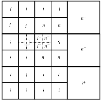
Figure 3: An adaptive, level-restricted tree: a typical leaf node at level $l$ in the hierarchy (away from the boundary) is marked by an $S$. Its colleagues are marked as $n$, its coarse neighbors as $n^{+}$ and its fine neighbors as $n^{-}$. The boxes marked by $i$ are the children of the colleagues of $S$’s parent (the so-called interaction list). The box marked $i^{+}$ is a colleague of $S$’s parent which does not touch $S$ and the boxes marked by $i^{-}$ are children of $S$’s colleagues which do not touch $S$. In the VFMM, the contributions to $S$ from boxes marked by $i,i^{+}$, or $i^{-}$ are accounted for using multipole and local expansions, while the contributions from boxes marked by $n,n^{+}$, or $n^{-}$ are handled using precomputed tables. The VFMM is a multi-level algorithm that computes all such interactions using $O(N)$ operations, where $N$ is the total number of points in the discretization.

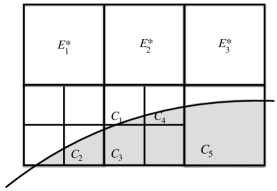
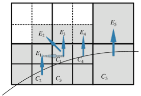
Figure 4: Cut squares $C_{1}-C_{5}$ on an adaptive, level-restricted quad-tree and their extensions from the domain $\Omega$ to a domain $E$ for which the VFMM can be used. (left): Note that, in the initial discretization, $C_{1}$ is the closest box to $E_{1}^{*}$ and $E_{2}^{*}$, while $C_{5}$ is closest to $E_{3}^{*}$. (right): Since $C_{1}$ is at a finer level, the boxes $E_{1}^{*}$ and $E_{2}^{*}$ are subdivided before extension, while $E_{3}^{*}$ is not - it is within the extension region for $C_{5}$. The arrows indicate the box from which the extension to the indicated exterior boxes is computed.

4.1 Function extension on a quad-tree and the VFMM

Suppose now that $\bar{S}_{i}$ is the extension square associated with the cut leaf square $S_{i}$. Using the method of Section 3.2, we obtain the $(\bar{K}-1)$th total order Chebyshev expansion of $f^{e}$ on $\bar{S}_{i}$ in the form

(24) $$f^{e}(\mathbf{x})=\sum\limits_{m+n<\bar{K}}\alpha^{i}_{m,n}T_{m}(x_{1})T_{n}(x_{2}),\quad\mathbf{x}=(x_{1},x_{2})\in\bar{S},$$

where $T_{m}(x)$ is the Chebyshev polynomial of degree $m$ scaled to the dimensions of $\bar{S}_{i}$. We then evaluate the expression Eq. 24 at every square in the extension list of $S_{i}$.

We carry out this procedure for all cut leaf squares in the discretization (Fig. 4). For leaf squares that don’t intersect the domain $\Omega$ and are not in any cut square’s extension list, we set $f^{e}$ to zero. The set of all regular leaf nodes, all cut leaf nodes (to which $f$ has been extended) and all extension squares defines the domain $E$ with non-zero data, to which the VFMM from [12] is applied, computing $\mathcal{V}_{E}[f^{e}]$ on the $K\times K$ Chebyshev grids for all leaf squares. At any point $\mathbf{x}$ in the closure of $\Omega$, it is straightforward to compute $\mathcal{V}_{E}[f^{e}](\mathbf{x})$ by interpolation of the Chebyshev expansion of the leaf node containing the point.

5 Boundary correction using a double layer potential

Having found a particular solution to the Poisson equation in $\Omega$, namely $\mathcal{V}_{E}[f^{e}]$, it remains to solve the Laplace equation (4) with modified Dirichlet data: $g(\mathbf{x})-\mathcal{V}_{E}[f^{e}](\mathbf{x})$. The contribution $g(\mathbf{x})$ is given by the user and we compute the contribution $\mathcal{V}_{E}[f^{e}](\mathbf{x})$ as described in the preceding section. For the remainder of this section we consider the interior problem for a simply connected domain. The modifications required to handle multiply connected domain or exterior problems are discussed in Section 2.

We solve (4) using the boundary integral equation Eq. 12 with a Nyström discretization [3]. For this, let $\{t^{G}_{j}\}_{j=1}^{N_{q}}$ and $\{w^{G}_{j}\}_{j=1}^{N_{q}}$ be the canonical Gauss-Legendre nodes and weights for the interval $[-1,1]$. Consider a panel $\Gamma_{i}$ in (4), parametrized as in (4). We let $\mathbf{y}_{ij}=\mathbf{y}(\boldsymbol{\gamma}_{i}(t^{G}_{j}))$, $\boldsymbol{\nu}_{ij}=\boldsymbol{\nu}(\mathbf{y}_{ij})$, $s_{ij}=\|\boldsymbol{\gamma}_{i}^{\prime}(t^{G}_{j})\|$, and $\sigma_{ij}$ be the approximation of $\sigma(\mathbf{y}_{ij})$. Applying Gauss-Legendre quadrature to the double layer potential yields

(25) $$\mathcal{D}[\sigma](\mathbf{x})=\int\limits_{\partial\Omega}\frac{\partial G(\mathbf{x}-\mathbf{y})}{\partial\boldsymbol{\nu}(\mathbf{y})}\sigma(\mathbf{y})\,\mathrm{d}s\approx\sum\limits_{i=1}^{N_{\Gamma}}\sum\limits_{j=1}^{N_{q}}\frac{\partial G(\mathbf{x},\mathbf{y}_{ij})}{\partial\boldsymbol{\nu}_{ij}}\sigma_{ij}s_{ij}w^{G}_{j},$$

since $\mathrm{ds}=\|\boldsymbol{\gamma}^{\prime}_{i}(t)\|\,\mathrm{d}t$. Recall that the double layer kernel is smooth on a smooth boundary, so that the approximation Eq. 25 has an error of the order $O(h^{2N_{q}}$ where $h=|\Gamma_{i}|/N_{q}$. Using this quadrature in our Nyström scheme applied to Eq. 12 yields the discrete linear system

(26) $$\frac{1}{2}\sigma_{i^{\prime}j^{\prime}}+\frac{1}{2\pi}\sum\limits_{i=1}^{N_{\Gamma}}\sum\limits_{j=1}^{N_{q}}\frac{\partial G(\mathbf{y}_{i^{\prime}j^{\prime}},\mathbf{y}_{ij})}{\partial\boldsymbol{\nu}_{ij}}\sigma_{ij}s_{ij}w^{G}_{j}=g(\mathbf{y}_{i^{\prime}j^{\prime}})-\mathcal{V}_{E}[f^{e}](\mathbf{y}_{i^{\prime}j^{\prime}}),$$

for $i^{\prime}=1,\ldots,N_{\Gamma}$ and $j^{\prime}=1,\ldots,N_{q}$. In matrix form, we write (26) as

$$(\boldsymbol{\mathrm{I}}+2\mathbf{D})\boldsymbol{\sigma}=2(\mathbf{g}-\mathbf{V}).$$

While the system matrix $\mathbf{D}$ is dense, it is well-conditioned and can be solved efficiently with GMRES. This follows from the fact that the underlying integral equation is an invertible Fredholm equation of the second kind, whose eigenvalues cluster at $(1,0)$ [33, 32, 47].) Furthermore, the matrix-vector multiplications required by GMRES can be computed using the original (“point”) FMM with $\mathcal{O}(N_{\Gamma}N_{q})$ operations, resulting in an optimal time solver [22, 25, 40].

Having solved the integral equation, we may evaluate the double layer potential Eq. 25 at all interior points using the point FMM [25]. Care must be taken, however, as $\mathbf{x}$ approaches the boundary $\partial\Omega$, since the kernel Eq. 11 is singular and the smooth Gauss-Legendre rule used above loses accuracy. Designing quadrature rules for this regime has been an active area of research, and there are several FMM-compatible methods available that restore precision, such as [31, 5, 4]. We use the Helsing-Ojala correction scheme [28] in this paper.

5.1 Error analysis

One of the advantages of potential theory is that it uncouples the discretization of the domain from that of the boundary and permits very simple error analysis. In computing the particular solution $\mathcal{V}_{E}[f^{e}]$, there are two sources of error. The first is the error $\epsilon_{f}$ made in the piecewise polynomial approximation of $f(\mathbf{x})$. Since the volume integral operator $\mathcal{V}_{E}$ is bounded, this contributes an error of the order $O(\epsilon_{f})$. The second is the error made in computing $\mathcal{V}_{E}[f^{e}]$ for that piecewise polynomial approximation $f^{e}$. The VFMM computes this exactly, up to the tolerance $\epsilon_{FMM}$ specified by the user. More complicated is the error in the double layer potential. Since this involves the solution of an integral equation, we can’t specify the accuracy a priori. We can say, however, that the order of accuracy of the solution is that of the underlying quadrature rule. This is a particular feature of second kind integral equations [3]. That is, we are guaranteed high order convergence from a high order accurate rule. We must also ensure that the right-hand side of the integral equation (26), namely $g(\mathbf{y})-\mathcal{V}_{E}[f^{e}](\mathbf{y})$, is well-resolved. This is a slightly subtle issue, since the function is cut off sharply at the boundary of the extension region $E$, which could introduce high-frequency content in the term $\mathcal{V}_{E}[f^{e}](\mathbf{y})$. Our algorithm mitigates this by ensuring that the corner points of the polygonal boundary $\partial E$ are pushed out at least a full leaf node away from the domain boundary $\partial\Omega$.

Remark 5.1.

One could also sample the curve more finely to ensure that a piecewise polynomial approximation of $g(\mathbf{y})-\mathcal{V}_{E}[f^{e}](\mathbf{y})$ is resolved to the desired precision. We have not investigated this issue in detail. In the present paper, we sample the boundary sufficiently finely that the error is dominated by the accuracy of the volume integral.

Remark 5.2.

For nonsmooth boundaries, we rely on the recent development of high order solvers that deal efficiently with corner singularities, such as [8, 27, 29]). The essential idea in these schemes is the use of dyadic refinement to the corner to overcome the induced singularity in the double layer density. We make use here of the RCIP method of [27] and refer the reader to the original paper for further details.

6 Numerical results

The bulk of the software for our function extension scheme is written in Julia 1.7.1 [6] and available at [18]. It can be used to generate the results in this section. Software for the boundary integral equation, the evaluation of the double layer potential, the RCIP scheme, and the RBF-QR algorithm have also been implemented in Julia. The latter is available at [20]. The full Poisson solver relies on several external packages: the VFMM [12] is written in Fortran and available at [13], fixed at eighth order accuracy. We set the FMM tolerance to $\epsilon_{FMM}=0.5\times 10^{-11}$. The “point” FMM we use is available at [49].

In our discretization, we set $K=8$ for the Chebyshev grids on leaf nodes, whether they are regular or cut. The number of Gaussians is set to $N_{\mathcal{G}}=66$, as discussed in Section 3.2. We have found this works well in practice to obtain eighth order accuracy. On the extension region, $\bar{S}$, we set $\bar{K}=12$. When it is resampled on the individual extension squares, however, we interpolate on $8\times 8$ Chebyshev grids, for compatibility with the VFMM. As the algorithm traverses the extension list, no square is written to more than once, making the extension step trivially parallel. On the boundary, we use $N_{q}=16$ Gauss-Legendre nodes for each panel. The number of panels $N_{\Gamma}$ is set to be sufficiently large that resolving the geometry does not dominate the error. That is, we pick $N_{\Gamma}$ to ensure that, on each panel, the $16$ point Gauss-Legendre expansion of $\|\boldsymbol{\gamma}\|$ is resolved to fifteen digits of accuracy.

In the following numerical experiments, we compute the solution at the subset of a uniform $100\times 100$ grid on $D$ that lie inside $\Omega$ for the interior problem, and outside $\Omega$ for the exterior problem. We measure the error in both the relative $\ell^{\infty}$ norm and the relative $\ell^{2}$ norm.

For convergence studies, we use a uniform quad-tree; thus, at level $l$ there are $N=8\cdot 2^{l}$ points in each dimension. All computations were carried out on a single core of a $4.2$ GHz Intel i$7-8620U$ with $16$ GB of memory.

6.1 The interior problem

For our first test, we consider the problem posed as Example $2$ in [2]. It involves a doubly connected domain with a right-hand side that has some very fine features with exact solution

(27) $$u(\mathbf{x})=\sin(10(x_{1}+x_{2}))+x_{1}^{2}-3x_{2}+8+\exp(-500x_{1}^{2}),\quad\mathbf{x}\in\Omega.$$

The two boundary components are specified in polar coordinates with $\theta\in[0,2\pi)$ and

$$r(\theta)=\sum_{j}(c_{j}\cos(j\theta)+d_{j}\sin(j\theta)).$$

The non-zero coefficients for the outer boundary $\partial\Omega_{0}$ are $c_{0}=0.25$, $d_{3}=c_{6}=c_{8}=c_{10}=0.01$ and $c_{5}=0.02$. The non-zero coefficients for the inner boundary $\partial\Omega_{1}$ are $c_{0}=0.05$ and $c_{2}=d_{3}=c_{5}=c_{7}=0.005$. (See Fig. 5.) We discretize $\partial\Omega_{0}$ with $200$ panels and $\partial\Omega_{1}$ with $180$ panels.

In Fig. 5, we observe the expected eighth order convergence as we refine the quad-tree uniformly. The $\ell^{\infty}$ error levels out after six levels of refinement at about eleven digits of accuracy, more or less the FMM tolerance $\epsilon_{FMM}$. The $\ell^{2}$ error continues to decrease for one more level, reaching twelve digits of accuracy. For comparison, we also plot the errors when the function extension is carried out exactly based on the exact solution (to the same region $E\supset\Omega$). We refer to this as the analytic extension. Note that we lose one to two digits of accuracy from our numerical scheme (although with sufficient refinement, the errors are the same).

We test the performance of the adaptive solver, using $\epsilon_{FMM}=0.5\times 10^{-11}$ for both the VFMM and in determining when the right-hand side is sufficiently resolved. As noted above, we also ensure that the dimensions of the cut squares are commensurate with the boundary panel size ($|\partial\Omega_{0}|/N_{\Gamma}$), which requires seven levels of refinement near the boundary. The resulting $\ell^{\infty}$ error is $2\times 10^{-11}$, with an $\ell^{2}$ error of $10^{-12}$. The full discretization requires $3361$ leaf squares, of which $339$ are cut, with a total of about $215,000$ points. The construction of the quad-tree, which includes labeling squares as cut, imposing the level-restriction, and imposing the extension-restriction, requires $0.3$ seconds. The precomputation steps in function extension - building the extension lists and identifying points as inside or outside - requires $0.7$ seconds. Creating the extension itself requires $0.4$ seconds, and the VFMM requires $0.2$ seconds. Finally, solving the integral equation and evaluating the double layer potential requires $0.7$ seconds. Note that, since seven levels of uniform refinement would require $N\sim 10^{3}$ points, adaptivity has yielded a factor of five improvement for the same accuracy. It is difficult to make a direct comparison with the scheme of [2], since they used a less smooth extension and relied on a fourth order VFMM. For the same example, however, ten times more points were needed to obtain an error of $10^{-8}$.

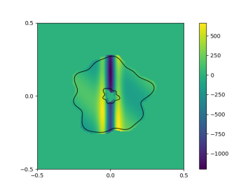
(a)

(b)

(c)

Figure 5: The doubly-connected interior problem of Section 6.1. (a) The extended function $f=\Delta u$ with $u$ given by Eq. 27 (with seven levels of refinement). (b) Pointwise error in the computed solution. (c) Convergence plot under uniform refinement (markers are from levels three to eight in the refinement process).

In a second test, we use the same exact solution $u$ from Eq. 27, but in the simply connected domain shown in Fig. 6. Using complex notation $z(\theta)=x(\theta)+iy(\theta)$, the boundary $\partial\Omega$ is given by

(28) $$z=0.17((2+0.5\sin(7\theta))\cos(\theta+0.5\sin(7\theta))+i((2+0.5\sin(7\theta))\sin(\theta+0.5\sin(7\theta))),$$

where $\theta\in[0,2\pi)$. We again observe the expected eighth order convergence, but with a larger constant for the error than for our first example.

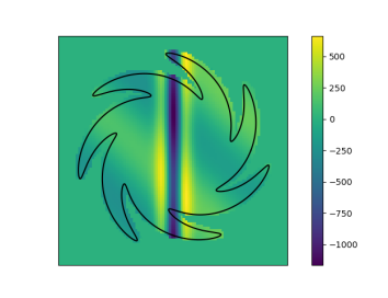
(a)

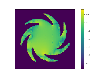
(b)

(c)

Figure 6: (a) Extended function $f=\Delta u$, with $u$ from Eq. 27, using seven levels of refinement. (b) Pointwise absolute error for solving the problem in Section 6.1. (c) Convergence plot as the quad-tree is uniformly refined. Here, we plot from three levels of refinement to eight levels of refinement.

6.2 The exterior problem

We turn now to a test for the exterior solver on a multiply connected domain (Fig. 7). Using complex notation again, we have

(29) $$z=R((1+a\cos(Nt))\exp(-it))+c_{1}+ic_{2},\quad\text{ for }t\in[0,2\pi).$$

For $\partial\Omega_{1}$ we set $R=0.12$, $a=0.3$, $N=5$, $c_{1}=0.186$, and $c_{2}=-0.15$. For $\partial\Omega_{2}$ we set $R=0.17$, $a=0.3$, $N=4$, $c_{1}=-0.21$, and $c_{2}=-0.03$, and for $\partial\Omega_{3}$ we set $R=0.2$, $a=0.2$, $N=3$, $c_{1}=0.2$, and $c_{2}=0.15$. We solve the Poisson equation on this domain with the exact solution

(30) $$u(\mathbf{x})=\sum\limits_{j=1}^{3}e^{-\|\mathbf{x}-\mathbf{y}_{j}\|^{2}/\beta_{j}}-10\log\left(\sqrt{(x_{1}+0.2)^{2}+x_{2}^{2}}\right),\quad\text{ for }\mathbf{x}\in\mathbb{R}^{2}\setminus(\bar{\Omega}_{1}\cup\bar{\Omega}_{2}\cup\bar{\Omega}_{3}),$$

where $\mathbf{y}_{1}=(0.1,0.07)$, $\beta_{1}=10^{-3}$, $\mathbf{y}_{2}=(0.09,-0.25)$, $\beta_{2}=10^{-3}/2.1$, $\mathbf{y}_{3}=(-0.21,-0.25)$, and $\beta_{3}=10^{-3}/4.5$ (see Fig. 7.) Note that the Gaussian centers $\{\mathbf{y}_{j}\}_{j=1}^{3}$ are interior to but close to the boundaries of the inclusions $\Omega_{j}$. Note also that we are seeking a solution which is growing logarithmically using the representation (19) for our integral equation solver, to impose the radiation condition $u(\mathbf{x})\rightarrow 10\log\|\mathbf{x}\|$ as $\|\mathbf{x}\|\rightarrow\infty$. Note, however, that the source distribution $f$ may itself have net “charge” $A^{e}=\iint_{E}f^{e}(\mathbf{y})\,\mathrm{d}\mathbf{y}$, so that the VFMM is computing a particular solution with growth $A^{e}\log\|\mathbf{x}\|$. Thus, in our integral equation solver, for the constraint conditions (20), we enforce

$$\int\limits_{\partial\Omega_{k}}\sigma(\mathbf{y})\,\mathrm{d}\mathbf{y}=0,\quad\,k=1,\ldots,N_{\Omega}-1\quad,\quad\sum_{k=1}^{N_{\Omega}}A_{k}=10-A^{e}.$$

The convergence plots in Fig. 7 show the expected eighth order convergence under uniform refinement.

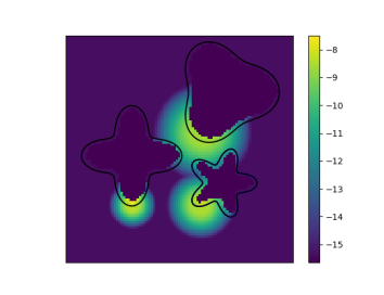
(a)

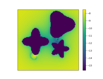
(b)

(c)

Figure 7: (a) Extended function $f=\Delta u$ on a logarithmic scale, with $u$ from Eq. 30, using seven levels of refinement. (b) Pointwise absolute error for solving the problem in Section 6.2. (c) Convergence plot as the quad-tree is uniformly refined, with markers at refinement levels three to nine.

6.3 Piecewise smooth boundaries

A good demonstration of the value of potential theory is the solution of the Poisson equation with a non-smooth boundary. Assuming that the source distribution is well-resolved by the user-provided grid, our extension scheme is agnostic as to the regularity of the boundary. Thus, let us suppose for simplicity that the solution and source density are both smooth on a square with side length $0.5$, centered at $(0.01,-0.02)$ and rotated $\pi/3$ radians, to avoid any benefit from alignment with the coordinate axes. We solve the interior problem with solution

(31) $$u(\mathbf{x})=-2\sum\limits_{j=1}^{4}\left(\mathrm{Ei}(\beta\|\mathbf{x}-\mathbf{x}_{j}\|^{2})+\log\|\mathbf{x}-\mathbf{x}_{j}\|^{2}\right),$$

with $\beta=800$, where $\mathrm{Ei}$ denotes the exponential integral function, $\mathbf{x}_{1}=(-0.35,-0.135)$, $\mathbf{x}_{2}=(-0.09,042)$, $\mathbf{x}_{3}=(0.445,0.09)$, and $\mathbf{x}_{4}=(0.135,-0.405)$ (see Fig. 8).

No modifications te the code is required for computing the volume potential $\mathcal{V}_{D}[f^{e}]$, but the double layer potential develops a singularity at the corners,so that we require a specialized quadrature scheme to achieve high order accuracy in computing the doulbe layer $\mathcal{D}[\sigma]$. For this, we make use of recursive(ly) compressed inverse preconditioning (RCIP) [27]. The results are shown in Fig. 8, where we again obtain the expected eighth order convergence. The code works equally well when the solution has corner singularities, so long as the source distribution is resolved by the quad-tree.

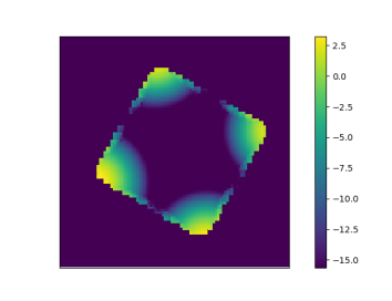
(a)

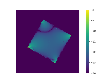
(b)

(c)

Figure 8: (a) Extended function $f=\Delta u$ on a logarithmic scale, with $u$ from Eq. 31, using seven levels of refinement. (b) Pointwise absolute error for solving the problem in Section 6.2. (c) Convergence plot as the quad-tree is uniformly refined, with markers at refinement levels three to eight.

6.4 Extension along lines

An alternate to our function extension scheme is to carry out one-dimensional extension along lines in the plane. Consider a star-shaped domain centered at the origin, as shown in Fig. 9, on which we seek to solve the interior problem with solution Eq. 27. For each point $\mathbf{x}$ outside $\Omega$ on the $\bar{K}\times\bar{K}$ grids for each $\bar{S}$, we extend along the line passing through the origin and $\mathbf{x}$. Assuming $\mathbf{x}\in\bar{S}$ for some cut cell $S$ of side length $L$, we assume we are given the data at eight uniformly-spaced interior nodes over a distance $L$ from the boundary. We then form the one-dimensional barycentric rational interpolant with Floater-Hormann weights [15], using the Julia implementation from [36]. We then evaluate the interpolant at $\mathbf{x}$. The results are shown in Fig. 9. Note that, using this extension method, provides errors of about the same magnitude as the analytic extension. Note also that we are not extending in the normal direction, but in the radial direction which intersects the boundary at some unspecified angle. The cost of this version of function extension is much less than that of a VFMM call. When considering geometries such as Fig. 6, a more careful implementation will be required to avoid caustics. We will return to this topic in the next section.

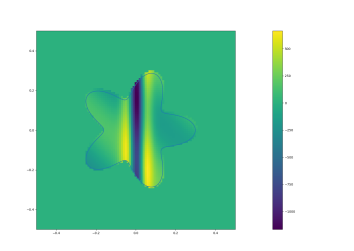
(a)

(b)

(c)

Figure 9: (a) Extended function $f=\Delta u$ on a logarithmic scale, with $u$ from Eq. 27, using seven levels of refinement. (b) and (c) are convergence plots for the relative $\ell^{\infty}$ error and the relative $\ell^{2}$ error, respectively, as the quad-tree is uniformly refined, with markers at refinement levels three to eight.

7 Conclusions

We have presented a potential theory-based solver for the Poisson equation in complicated two-dimensional geometries. To avoid computing a volume potential over the actual domain, which involves complicated quadratures over cut leaf nodes in a quad-tree discretization, we have developed a fast, high-order scheme to extend the source density smoothly to a slightly larger region where a volume integral FMM (VFMM) can be applied [12]. The VFMM computes a volume integral in linear time on an adaptive quad-tree, assuming that the source distribution is available on a tensor product grid for every leaf node in the tree. Unlike many earlier function extension schemes, we do not require the extended function to decay smoothly to zero. It is sufficient for it to be extended a sufficient distance from the domain boundary (on the order of a single cut square width). Having computed the volume potential, an auxiliary integral equation is solved to impose the desired boundary (and radiation) condition.

The order of convergence of our scheme is dictated by the underlying discretization, not the extension method, since we can adjust the order of accuracy of our Gaussian interpolant to match that of the underlying scheme. To make our extension efficient, we designed a single, universal interpolation matrix which can be precomputed and used for every cut leaf node which is intersected by the domain boundary. From the universal interpolation matrix, rows are extracted corresponding to data that lies in the domain interior. This leads to a small least squares problem that is solved by $QR$ factorization on each cut square. Unlike the earlier high-order extension method of [21], the present scheme visits each extension square once, without blending, making it much simpler to implement in parallel. Furthermore, the extension scheme does not rely on the smoothness of the boundary - just on being resolved by the user-provided data. The robustness, order of convergence, and accuracy of the scheme have been demonstrated with several numerical examples.

For our interior problem, with 11 digits of accuracy and eighth order convergence, the VFMM itself runs at about 1M points/sec/core and the RBF-based function extension runs at about 500,000 points/sec/core. The integral equation cost should be negligible (it is linear scaling in the number of boundary points, but sublinear in the total number of unknowns). It dominates here, since we rely on a non-optimized iterative FMM-based scheme, but the full solver still requires only about two seconds for a problem with more than 200,000 unknowns. We expect that with some modest modifications, the full solver should achieve a throughput of close to 500,000 points/sec/core.

A natural extension of the method presented here is to the three-dimensional case. The main ingredients are available, such as high performance, parallelized VFMM libraries [37] and layer potential FMMs for boundary integral equations [24]. However, it remains to be determined how well the RBF-QR algorithm performs in three dimensions [17]. If the constants associated with the RBF-QR approach are too large, our preliminary experiments, presented in Section 6.4, suggest that one-dimensonal extension may be equally effective and faster. We have begun exploring the extension method of [11], which appears to be just as efficient as rational approximation, both in terms of speed and accuracy. We suspect that, for robustness, this should always be done in the normal direction and we are actively investigating this approach. Finally, we should note that our function extension scheme is unrelated to the governing PDE - it can be used with any potential-theoretic approach to boundary value problems in complicated domains when fast solvers like the VFMM are available.

References

- [1] T. G. Anderson, H. Zhu, and S. Veerapaneni, A fast, high-order scheme for evaluating volume potentials on complex 2D geometries via area-to-line integral conversion and domain mappings, 2022, https://arxiv.org/abs/2203.05933.
- [2] T. Askham and A. Cerfon, An adaptive fast multipole accelerated Poisson solver for complex geometries, J. Comput. Phys., 344 (2017), pp. 1–22.
- [3] K. E. Atkinson, The Numerical Solution of Integral Equations of the Second Kind, Cambridge Monographs on Applied and Computational Mathematics, Cambridge University Press, 1997, https://doi.org/10.1017/CBO9780511626340.
- [4] A. Barnett, B. Wu, and S. Veerapaneni, Spectrally accurate quadratures for evaluation of layer potentials close to the boundary for the 2D Stokes and Laplace equations, SIAM Journal on Scientific Computing, 37 (2015), pp. B519–B542, https://doi.org/10.1137/140990826, https://doi.org/10.1137/140990826, https://arxiv.org/abs/https://doi.org/10.1137/140990826.
- [5] A. H. Barnett, Evaluation of layer potentials close to the boundary for Laplace and Helmholtz problems on analytic planar domains, SIAM Journal on Scientific Computing, 36 (2014), pp. A427–A451, https://doi.org/10.1137/120900253, https://doi.org/10.1137/120900253, https://arxiv.org/abs/https://doi.org/10.1137/120900253.
- [6] J. Bezanson, A. Edelman, S. Karpinski, and V. B. Shah, Julia: A fresh approach to numerical computing, SIAM review, 59 (2017), pp. 65–98, https://doi.org/10.1137/141000671.
- [7] J. P. Boyd, A comparison of numerical algorithms for Fourier extension of the first, second, and third kinds, Journal of Computational Physics, 178 (2002), pp. 118–160.
- [8] J. Bremer, V. Rokhlin, and I. Sammis, Universal quadratures for boundary integral equations on two-dimensional domains with corners, J. Comput. Phys., 229 (2010), pp. 8259–8280.
- [9] O. P. Bruno and J. Paul, Two-dimensional Fourier continuation and applications, SIAM. J. Sci. Comput., 44 (2022), pp. A964–A992, https://doi.org/10.1137/20M1373189, https://doi.org/10.1137/20M1373189, https://arxiv.org/abs/https://doi.org/10.1137/20M1373189.
- [10] R. Coifman, P. Jones, and S. Semmes, Two elementary proofs of the boundedness of Cauchy integrals on Lipschitz curves, J. Am. Math. Soc., 2 (1989), pp. 553–564.
- [11] C. Epstein and S. Jiang, A stable, efficient scheme for function extensions on smooth domains in , 2022, https://doi.org/10.48550/ARXIV.2206.11318.
- [12] F. Ethridge and L. Greengard, A new fast-multipole accelerated Poisson solver in two dimensions, SIAM J. Sci. Comput., 23 (2002), pp. 741–760.
- [13] F. Ethridge, L. Greengard, M. Rachh, and S. Jiang, vfmm2d. https://github.com/mrachh/boxcode2d-legacy.
- [14] L. Evans, Partial Differential Equations, Graduate studies in mathematics, American Mathematical Society, 1998, https://books.google.com/books?id=5Pv4LVB_m8AC.
- [15] M. S. Floater and K. Hormann, Barycentric rational interpolation with no poles and high rates of approximation, Numer. Math., 107 (2007), p. 315–331, https://doi.org/10.1007/s00211-007-0093-y, https://doi.org/10.1007/s00211-007-0093-y.
- [16] G. B. Folland, Introduction to Partial Differential Equations: Second Edition, Princeton University Press, 1995, https://doi.org/doi:10.1515/9780691213033.
- [17] B. Fornberg, E. Larsson, and N. Flyer, Stable computations with Gaussian radial basis functions, SIAM J. Sci. Comput., 33 (2011), pp. 869–892.
- [18] F. Fryklund, bieps2d. https://github.com/fryklund/bieps2d. Accessed: 2022-07-25.
- [19] F. Fryklund, M. C. A. Kropinski, and A.-K. Tornberg, An integral equation-based numerical method for the forced heat equation on complex domains, Adv. Comput. Math, 46 (2020), pp. 1–36.
- [20] F. Fryklund and E. Larsson, RBF-QR. https://www.it.uu.se/research/scientific_computing/software/rbf_qr. Accessed: 2021-12-10.
- [21] F. Fryklund, E. Lehto, and A.-K. Tornberg, Partition of unity extension of functions on complex domains, J. Comput. Phys., 375 (2018), pp. 57–79.
- [22] A. Greenbaum, L. Greengard, and G. McFadden, Laplace’s equation and the Dirichlet-Neumann map in multiply connected domains, J. Comput. Phys., 105 (1993), pp. 267–278, https://doi.org/https://doi.org/10.1006/jcph.1993.1073.
- [23] L. Greengard and J.-Y. Lee, A direct adaptive Poisson solver of arbitrary order accuracy, Journal of Computational Physics, 125 (1996), pp. 415–424.
- [24] L. Greengard, M. O’Neil, M. Rachh, and F. Vico, Fast multipole methods for the evaluation of layer potentials with locally-corrected quadratures, Journal of Computational Physics: X, 10 (2021), p. 100092, https://doi.org/https://doi.org/10.1016/j.jcpx.2021.100092, https://www.sciencedirect.com/science/article/pii/S2590055221000093.
- [25] L. Greengard and V. Rokhlin, A fast algorithm for particle simulations, J. Comput. Phys., 73 (1987), pp. 325–348.
- [26] R. B. Guenther and J. W. Lee, Partial Differential Equations of Mathematical Physics and Integral Equations, Prentice Hall, 1988.
- [27] J. Helsing, Solving integral equations on piecewise smooth boundaries using the RCIP method: A tutorial, Abstr. Appl. Anal., 2013 (2013), pp. 1 – 20, https://doi.org/10.1155/2013/938167.
- [28] J. Helsing and R. Ojala, On the evaluation of layer potentials close to their sources, J. Comput. Phys., 227 (2008), pp. 2899–2921, https://doi.org/10.1016/j.jcp.2007.11.024.
- [29] J. G. Hoskins, V. Rokhlin, and K. Serkh, On the numerical solution of elliptic partial differential equations on polygonal domains, SIAM J. Sci. Comput., 41 (2019), pp. A2552–A2578.
- [30] O. D. Kellogg, Foundations of Potential Theory, Springer, 1929, http://eudml.org/doc/203661.
- [31] A. Klöckner, A. Barnett, L. Greengard, and M. O’Neil, Quadrature by expansion: A new method for the evaluation of layer potentials, Journal of Computational Physics, 252 (2013), pp. 332–349, https://doi.org/https://doi.org/10.1016/j.jcp.2013.06.027, https://www.sciencedirect.com/science/article/pii/S0021999113004579.
- [32] R. Kress, Linear Integral Equations, Applied Mathematical Sciences, 82, Springer, 3rd ed. 2014.. ed., 2014.
- [33] E. Kreyszig, Introductory Functional Analysis with Applications, Wiley classics library, Wiley India Pvt. Limited, 2007, https://books.google.com/books?id=osXw-pRsptoC.
- [34] E. Larsson and B. Fornberg, Theoretical and computational aspects of multivariate interpolation with increasingly flat radial basis functions, Comput. Math. with Appl., 49 (2005), pp. 103–130, https://doi.org/https://doi.org/10.1016/j.camwa.2005.01.010, https://www.sciencedirect.com/science/article/pii/S0898122105000118.
- [35] E. Larsson, V. Shcherbakov, and A. Heryudono, A least squares radial basis function partition of unity method for solving PDEs, SIAM J. Sci. Comput., 39 (2017), pp. A2538–A2563, https://doi.org/10.1137/17M1118087, https://doi.org/10.1137/17M1118087, https://arxiv.org/abs/https://doi.org/10.1137/17M1118087.
- [36] D. MacMillen, BaryRational. https://github.com/macd/BaryRational.jl. Accessed: 2022-07-20.
- [37] D. Malhotra and G. Biros, PVFMM: A parallel kernel independent FMM for particle and volume potentials, Commun. Comput. Phys., 18 (2015), p. 808–830.
- [38] A. McKenney, L. Greengard, and A. Mayo, A fast Poisson solver for complex geometries, Journal of Computational Physics, 118 (1995), pp. 348–355.
- [39] S. G. Mikhlin, Integral Equations, Pergammon, 1957.
- [40] V. Rokhlin, Rapid solution of integral equations of classical potential theory, J. Comput. Phys., 60 (1985), pp. 187–207.
- [41] R. Schaback, Multivariate interpolation by polynomials and radial basis functions, Constr. Approx., 21 (2005), pp. 293–317, https://doi.org/10.1007/s00365-004-0585-2.
- [42] D. Shirokoff and J. Nave, A sharp-interface active penalty method for the incompressible Navier–Stokes equations, J. Sci. Comput., 62 (2015), pp. 53–77, https://doi.org/10.1007/s10915-014-9849-6.
- [43] D. B. Stein, Spectrally accurate solutions to inhomogeneous elliptic PDE in smooth geometries using function intension, 2022, https://doi.org/10.48550/ARXIV.2203.01798.
- [44] D. B. Stein, R. D. Guy, and B. Thomases, Immersed boundary smooth extension: A high-order method for solving PDE on arbitrary smooth domains using Fourier spectral methods, Journal of Computational Physics, 304 (2016), pp. 252–274, https://doi.org/https://doi.org/10.1016/j.jcp.2015.10.023, https://www.sciencedirect.com/science/article/pii/S0021999115006877.
- [45] D. B. Stein, R. D. Guy, and B. Thomases, Immersed boundary smooth extension (IBSE): A high-order method for solving incompressible flows in arbitrary smooth domains, J. Comput. Phys., 335 (2017), pp. 155–178, https://doi.org/https://doi.org/10.1016/j.jcp.2017.01.010, https://www.sciencedirect.com/science/article/pii/S0021999117300207.
- [46] H. Sundar, R. S. Sampath, and G. Biros, Bottom-up construction and balance refinement of linear octrees in parallel, SIAM J. Sci. Comput., 30 (2008), pp. 2675–2708.
- [47] L. Trefethen and D. Bau, Numerical Linear Algebra, Other Titles in Applied Mathematics, Society for Industrial and Applied Mathematics, 1997, https://books.google.com/books?id=4Mou5YpRD_kC.
- [48] G. Verchota, Layer potentials and regularity for the Dirichlet problem for Laplace’s equation in Lipschitz domains, J. Funct. Anal., 59 (1984), pp. 572–611.
- [49] L. G. Z. Gimbutas, FMMLIB2D. https://github.com/zgimbutas/fmmlib2d. Accessed: 2021-12-10.