Translating Solitons in Generalised Robertson-Walker Geometries

Abstract.

We generalise the notion of translating solitons in Generalised Robertson-Walker sapcetimes, which come equipped with a natural conformal Killing time-like vector field. We single out three one-parameter families of warping functions for which these objects exist, and we fully classify the corresponding Grim Reapers - translation-invariant solitons- for a large family of Riemannian fibres.

Key words: Generalised Robertson-Walker, translating solitons, warped, spacetime, mean curvature flow, Grim Reapers, Lorentzian

MSC: 53C44; 53C21; 53C42; 53C50.

1. Introduction

Since the seminal work of Huisken [14], solutions to the mean curvature flow in $\mathbb{R}^{n}$ have been extensively studied. Solitons, which are special solutions evolving by a group of conformal transformations of $\mathbb{R}^{n}$, have received particular attention [2, 5, 6, 11, 13, 20]. If the group is a subgroup of translations of the ambient space, these solutions are called translating solitons or translators, and satisfy the simplified mean curvature flow equation

$$H=X^{\perp},$$

where the translating direction $X\in\mathbb{R}^{n}$ is a constant vector. Translating solitons are of great importance not only because they are eternal solutions to the mean curvature flow, but also because they appear naturally in the study of singularities [12, 25] and are intimately related to the theory of minimal surfaces. For example, it is well-known that they are equivalent to minimal surfaces for a conformal metric [15]. In the last years, many families of translators have been constructed using various techniques [6, 20, 24]. Of particular interest are the translating solitons which are invariant under a group of isometries of the ambient space. In the case of translational or rotational invariance, they have been completely classified in [20] and [2, 6]. For the first case, the only non-trivial example was the Grim Reaper curve in the Euclidean plane. In higher dimensions, Grim Reapers are essentially the product of a Grim Reaper curve and a 2-codimensional hyperplane orthogonal to it.

Recently, generalisations of translating solitons to other ambient spaces have emerged. In [16, 9] the authors consider the general situation where the ambient manifold is a Riemannian product $(P\times\mathbb{R},g_{P}+dt^{2})$ of a Riemannian manifold with the real line. An obvious translating direction is given by the parallel vector field $\partial_{t}$, and one can naturally consider graphical solitons over $P$. Generalising this idea to Lorentzian products, the last two authors gave in [18] new examples of translators in Minkowski space. In particular, they completely classified those translating solitons which are rotationally symmetric or, in other words, those invariant by the cohomogeneity-one action of the special orthogonal and orthochronal Lie groups. To do so, they use the general fact that the existence of such a cohomogeneity-one action ensures the manifold to admit a (pseudo-)Riemannian submersion to a one-dimensional base manifold, hence reducing the PDE to an ODE.

Going one step further, in [9], the authors actually consider a definition of translating solitons in the direction of an arbitrary vector field, although these solutions might not be solutions to the mean curvature flow in the classical sense. In this context, solutions associated with conformal Killing vector fields are obvious examples of study.

Our aim is to go further in this study, inspired by the translating solitons in a classical sense, but in a larger class of Lorentzian manifolds, using similar techniques to the ones in [18]. Instead of a (pseudo-)Riemannian product, we consider the well-established family of Generalised Robertson-Walker (GRW) spacetimes $M=N\times I$, with warped product metric $b(t)g_{N}-dt^{2}$, for $(N,g_{N})$ a Riemannian manifold and $b:I\to(0,+\infty)$. Introduced in [1], these spaces are of particular interest in Physics, where they serve to construct famous models of the universe, including among others homogeneous, isotropic and expanding or contracting cases. The vector field $b\,\partial_{t}$ is obviously a conformal Killing vector field, and we can consider translators in its direction. We also point out that in [10] the authors study long-time existence of solutions to the mean curvature flow in another family of GRW spacetimes.

This paper is structured as follows. In Section 2, we recall some preliminary definitions and explain the setup. In Section 3, GRW spacetimes are introduced. We consider a function $u$ defined on an open subset of the base manifold $M$ and, by using the flow of $\partial_{t}$, we construct graphical hypersurfaces in our GRW spacetime. We ask this hypersurface to satisfy the equation

(1.1) $$(b\,\partial_{t})^{\perp}=\vec{H}\,,$$

where $\vec{H}$ is the mean curvature vector of the hypersurface and $(b\,\partial_{t})^{\perp}$ is the orthogonal projection of $b\,\partial_{t}$ to the normal bundle of the hypersurface. We obtain the corresponding PDE that $u$ must satisfy in Proposition 3.6. Then, we reduce this PDE to an ODE by means of an appropriate submersion to a 1-dimensional base. Next, by considering $N=P\times\mathbb{R}$, where $P$ is any Riemannian manifold, we focus on the Grim Reaper family. In addition, a reasonable hypothesis to obtain the existence of such solutions is to restrict ourselves to two families of warping functions. For these functions, we compute the sectional curvature of the associated GRW spacetimes in order to obtain some extra information. And we check if these spaces satisfy the Null Convergence Condition. In Section 4, we completely classify the Grim Reapers in their corresponding GRW sapcetimes – vid. Theorem 4.15.

2. Preliminaries

Let $\left(M,g_{M}\right)$ and $\left(N^{n},g_{N}\right)$ be pseudo-Riemannian manifolds. Let $\varepsilon>0$. A smooth family of smooth embeddings $\left\{F_{t}\colon\left(N,g_{N}\right)\to\left(M,g_{M}\right)\colon t\in(-\varepsilon,\varepsilon)\right\}$ is said to be a solution to the mean curvature flow if, and only if, for all $t\in(-\varepsilon,\varepsilon)$, the pullback $F_{t}^{*}g_{M}$ is non-degenerate and

$$\left(\frac{\partial F_{t}}{\partial t}\right)^{\perp}=\vec{H}_{t}\,,$$

where $\vec{H}_{t}$ is the mean curvature vector of $F_{t}$. Recall that, if $\left(e_{1},\dots,e_{n}\right)$ is a local $(F_{t}^{*}g_{M})$-orthonormal frame of $N$, with $g\left(\left(F_{t}\right)_{*}e_{i},\left(F_{t}\right)_{*}e_{j}\right)=\varepsilon_{i}\delta_{ij}$, for $i,j=1,\dots,n$, then $\vec{H_{t}}$ is defined as

(2.1) $$\vec{H}_{t}=\sum_{i=1}^{n}\varepsilon_{i}\left(\nabla^{M}_{\left(F_{t}\right)_{*}e_{i}}\left(F_{t}\right)_{*}e_{i}\right)^{\perp}\,,$$

where $\nabla^{M}$ is the Levi-Civita connection of $(M,g_{M})$ – along the paper, we will denote by $\nabla^{P}$ the Levi-Civita connection of a given pseudo-Riemannian manifold $(P,g_{P})$ – and $\perp$ denotes orthogonal projection to the normal bundle of $F_{t}$. Now suppose we have a smooth family of conformal maps $\left\{C_{t}\colon\left(M,g_{M}\right)\to\left(M,g_{M}\right)\colon t\in(-\varepsilon,\varepsilon)\right\}$ and a fixed pseudo-Riemannian immersion $F_{0}\colon\left(N,g_{N}\right)\to\left(M,g_{M}\right)$. We say that $F_{0}$ defines a soliton with respect to the family $\{C_{t}\colon t\in(-\varepsilon,\varepsilon)\}$ if, and only if, the family $\left\{F_{t}=C_{t}\circ F_{0}\colon t\in(-\varepsilon,\varepsilon)\right\}$ is a solution to the mean curvature flow.

Suppose that $M=N\times I$, with $I\subseteq\mathbb{R}$ an open interval, and that $g_{M}(x,t)=\varphi(x,t)g_{N}(x)+\psi(x,t)dt^{2}$ is a pseudo-Riemannian metric on $M$, for some smooth functions $\varphi,\psi\colon N\times I\to\mathbb{R}$. These spaces provide us with:

1. a natural direction in which translate, namely the $I$-direction;

2. a natural class of candidates to solitons, namely graphs of functions $N\to I$.

For some choices of the functions $\varphi$ and $\psi$, one can find a conformal Killing vector field on $M$, whose flow will provide us with a one-parameter family of conformal maps with respect to which one can try to find functions $N\to I$ whose graph is a soliton. In this sense, we are generalising the classical notion of translating soliton [9].

In [18], Lawn and Ortega studied the case where $\varphi$ is constant equal to $1$ and $\psi$ is also constant equal to $\pm 1$. We will now look at other choices of $\varphi$ and $\psi$ which have interest in other areas of Mathematics and Physics.

3. Generalised Robertson-Walker Geometries

We now turn our attention to Generalised Robertson-Walker geometries, which in our setting correspond to taking $\psi$ constant equal to $-1$ and $\varphi=\tilde{\varphi}\circ\pi_{2}$, where $\tilde{\varphi}\colon I\to(0,\infty)$ is smooth and $\pi_{2}$ denotes the projection to the second factor. These spaces were introduced by Alías, Romero and Sánchez in [1], and have been widely studied [4, 17].

Let $\left(N,g_{N}\right)$ be an $n$-dimensional Riemannian manifold, $I\subseteq\mathbb{R}$ an open interval and $b\colon I\to\left(0,+\infty\right)$ a smooth function. A Generalised Robertson-Walker spacetime (GRW) with base $I$, fibre $\left(N,g_{N}\right)$ and warping function $b$ is the product manifold $M=N\times I$ endowed with the metric

$$g=g_{M}=b(t)^{2}g_{N}-dt^{2}\,,$$

where $t$ is the coordinate in $I$. We will denote this space by $\mathcal{RW}\left(N,g_{N},I,b\right)$.

When $M$ is a real spaceform, these spaces are used in Physics to model a homogeneous, isotropic and expanding or contracting universe, vid. [4] and references therein.

Following the previously discussed ideas, these spaces come naturally equipped with a conformal Killing vector field.

Lemma 3.1.

The vector field $X\coloneqq b(t)\partial_{t}$ is a conformal Killing vector field on $\left(M,g\right)=\mathcal{RW}\left(N,g_{N},I,b\right)$. More specifically,

$$\mathcal{L}_{X}g=2b^{\prime}g.\qed$$

Lemma 3.1 provides us with a one-parameter family of conformal diffeomorphisms between open subsets of $M$, namely the flow $\Phi_{s}$ of the vector field $X=b(t)\partial_{t}$. Note that, for all $x\in N$ and $t$ sufficiently small,

$$\Phi_{t}(x,s)=(x,A(s,t)),$$

where $A(s,t)$ satisfies

(3.1) $$\left\{\begin{array}[]{ll}A(s,0)=s,\\ \frac{\partial A}{\partial t}(s,t)=b\left(A(s,t)\right).\\ \end{array}\right.$$

We will restrict our attention to hypersurfaces of $M$ which are graphs of functions $N\to I$, as this is the generic case. Let $\Omega\subseteq N$ be open, precompact and connected, and let $u\in C^{2}(\Omega,I)$. Then, there exists $\varepsilon>0$ such that the flow $\Phi_{t}$ of $X$ is defined in $\Omega$ for all $t\in(-\varepsilon,\varepsilon)$. For $t\in(-\varepsilon,\varepsilon)$, consider

$$\begin{split}F_{t}\colon\Omega&\rightarrow N\times I=M\\ x&\mapsto\Phi_{t}\left(x,u(x)\right)=(x,u_{t}(x))\end{split}\hskip 5.69046pt,$$

where $u_{t}(x)\coloneqq A\left(u(x),t\right)$. $F_{t}$ is an embedding for every $t$, as it is a graph map. Suppose further that $F_{0}^{*}g$ is non-degenerate – and hence $F_{t}^{*}g$, for all sufficiently small $t$. In this setting, we can establish an important definition:

Definition 3.2.

We say that $F\coloneqq F_{0}$ is an $X$-soliton if, and only if, for every $x\in\Omega$ and $t\in(-\varepsilon,\varepsilon)$,

(3.2) $$\left(b\circ u_{t}\right)(x)\,\partial_{t}^{\perp}(x,u_{t}(x))=\vec{H_{t}}(x,u_{t}(x))\,,$$

where $\vec{H_{t}}$ is the mean curvature of the pseudo-Riemannian immersion $F_{t}$. As in [9], we say that $F$ defines a pointwise $X$-soliton if (3.2) is satisfied for $t=0$.

In [10], de Lira and Roing considered some natural conditions for the longtime existence of the mean curvature flow in a class of GRW spacetimes. In Section 3.3 we will introduce another class of such spacetimes which, as we shall see in Section 3.4.2, does not satisfy all their hypotheses.

3.1. Characterising PDE

In this section we will obtain the PDE characterising the property of being a (pointwise) $X$-soliton in a GRW spacetime.

Remark 3.3.

For the moment, for simplicity, we will work only with the graph map $F$ of a function $u\in\mathcal{C}^{2}(\Omega,I)$, where $\Omega\subseteq N$ is open, precompact and connected, to find a more explicit expression for equation (3.2). We will find a PDE for $u$ characterising the property of $F$ being a pointwise $X$-soliton. The $X$-soliton case will result from substituting $u$ with $u_{t}$ and $F$ with $F_{t}$, and imposing that the PDE be satisfied for all $t$ in a suitable neighbourhood of $0$.

Note that, under the usual identifications, if $X\in\Gamma\left(\operatorname{T}N\right)$, then

$$F_{*}X=\left(X,0\right)+g_{N}\left(\nabla u,X\right)\partial_{t}=\left(X,g_{N}\left(\nabla u,X\right)\right)\,.$$

Also, the vector field

$$\frac{1}{b(u(x))^{2}}\left(\nabla u(x),0\right)+\partial_{t}$$

is normal to $F$.

Lemma 3.4.

Under the previous notation and hypotheses, for all $x$ in $\Omega$ the quantity

$$\varepsilon^{\prime}(x):=\operatorname{sign}\left(\frac{\absolutevalue{\nabla u(x)}^{2}}{b(u(x))^{2}}-1\right)\in\{\pm 1\}\,,$$

and it is constant.

Proof.

Indeed, suppose it is not. Then, as $\Omega$ is connected, there exists $x\in\Omega$ such that

(3.3) $$\frac{\absolutevalue{\nabla u(x)}^{2}}{b(u(x))^{2}}-1=0.$$

In such case, we would have for every tangent vector $Y\in\operatorname{T}_{x}M$ that

$$\left(F^{*}g\right)\left(\nabla u(x),Y\right) =g\left(F_{*}\nabla u(x),F_{*}Y\right)$$

$$=g\left(\left(\nabla u(x),0\right)+\absolutevalue{\nabla u(x)}^{2}\partial_{t},Y+g_{N}\left(\nabla u(x),Y\right)\partial_{t}\right)$$

$$=b(u(x))^{2}g_{N}\left(\nabla u(x),Y\right)-\absolutevalue{\nabla u(x)}^{2}g_{N}\left(\nabla u(x),Y\right)$$

$$=0.$$

But, by hypothesis, $F^{*}g$ is non-degenerate, so this would imply that $\nabla u(x)=0$, which in turn would imply that $\absolutevalue{\nabla u(x)}^{2}=0$, which contradicts (3.3). ∎

So the vector field

(3.4) $$\nu(x)=\frac{1}{W(x)}\left(\frac{1}{b(u(x))^{2}}\left(\nabla u(x),0\right)+\partial_{t}\right),\,x\in\Omega\,,$$

where

(3.5) $$W(x)=\sqrt{\varepsilon^{\prime}(x)\left(\frac{\absolutevalue{\nabla u(x)}^{2}}{b(u(x))^{2}}-1\right)}\,,$$

is a normal vector field to $F$ with $g(\nu,\nu)=\varepsilon^{\prime}$.

In [8], Hernandes de Lima computed the mean curvature vector of $F$, obtaining

(3.6) $$g\left(\vec{H},\nu\right)=-\text{div}\left(\frac{\nabla u}{(b\circ u)^{2}W}\right)-\frac{(b^{\prime}\circ u)}{(b\circ u)W}\left(n+\frac{\absolutevalue{\nabla u}^{2}}{(b\circ u)^{2}}\right),$$

where $n=\dim(N)$.

Theorem 3.5.

Under the previous hypotheses and notation, $F$ is a pointwise $X$-soliton if, and only if, $u$ satisfies the following partial differential equation:

(3.7) $$\text{div}\left(\frac{\nabla u}{\left(b\circ u\right)\,W}\right)=\frac{1}{W}\left[\left(b\circ u\right)^{2}-n\left(b^{\prime}\circ u\right)\right].$$

Proof.

$\vec{H}=(b\circ u)\partial_{t}^{\perp}\text{ if and only if }g\left(\vec{H},\nu\right)=(b\circ u)g\left(\partial_{t}^{\perp},\nu\right)=(b\circ u)g\left(\partial_{t},\nu\right)=-(b\circ u)/W$, as $\left(\nabla u,0\right)\perp\partial_{t}$. But, using equation (3.6),

$$g\left(\vec{H},\nu\right)=-\text{div}\left(\frac{\nabla u}{(b\circ u)^{2}W}\right)-\frac{(b^{\prime}\circ u)}{(b\circ u)W}\left(n+\frac{\absolutevalue{\nabla u}^{2}}{(b\circ u)^{2}}\right)$$

$$=\frac{-1}{(b\circ u)}\text{div}\left(\frac{\nabla u}{(b\circ u)W}\right)-g_{N}\left(\nabla\left(\frac{1}{(b\circ u)}\right),\frac{\nabla u}{(b\circ u)W}\right)-$$

$$-\frac{(b^{\prime}\circ u)}{(b\circ u)W}\left(n+\frac{1}{(b\circ u)^{2}}\absolutevalue{\nabla u}^{2}\right)$$

$$=\frac{-1}{(b\circ u)}\left(\text{div}\left(\frac{\nabla u}{(b\circ u)W}\right)+\frac{n(b^{\prime}\circ u)}{W}\right),$$

which yields the result. ∎

As explained in Remark 3.3, we obtain the characterisation of $X$-solitons from pointwise $X$-solitons by substituting $u_{t}$ for $u$ in (3.7), obtaining the following:

Proposition 3.6.

The family $\{F_{t}\colon t\in(-\varepsilon,\varepsilon)\}$ defines an $X$-soliton if, and only if, for each $x\in\Omega$ and $t\in(-\varepsilon,\varepsilon)$:

(3.8) $$\text{div}\left(\frac{\nabla u}{\left(b\circ u\right)\,W}\right)(x)=\frac{1}{W(x)}\left[\left(b(u_{t}(x))\right)^{2}-n\left(b^{\prime}(u_{t}(x))\right)\right]\,.$$

Proof.

Note that, by the chain rule,

$$\nabla u_{t}=\nabla\left(A\left(u(x),t\right)\right)=\partial_{1}A\left(u(x),t\right)\nabla u\,,$$

where $\partial_{1}$ denotes partial derivative with respect to the first variable. Let us compute $\partial_{1}A\left(u(x),t\right)$. By definition, $A$ satisfies (3.1). Hence, for every $t,s$,

$$\int_{A(s,0)}^{A(s,t)}\frac{1}{b(y)}dy=\int_{0}^{t}dr=t\,.$$

Thus, by Leibniz’s integral rule,

$$0 =\frac{\partial}{\partial s}t=\frac{\partial}{\partial s}\left(\int_{A(s,0)}^{A(s,t)}\frac{1}{b(y)}dy\right)=\frac{1}{b\left(A(s,t)\right)}\frac{\partial A}{\partial s}(s,t)-\frac{1}{b\left(A(s,0)\right)}\frac{\partial A}{\partial s}(s,0)\,,$$

and hence

$$\frac{\partial A}{\partial s}(s,t)=\frac{b\left(A(s,t)\right)}{b(s)}.$$

So we have that

$$\nabla u_{t}=\frac{b\circ u_{t}}{b\circ u}\nabla u\,.$$

Using this, a straightforward computation shows that $W_{t}=W$ for every $t$, and the result follows. ∎

Remark 3.7.

If $b=1$, equation (3.8) coincides with the equation found by Lawn and Ortega in [18].

3.2. Reduction to an ODE

We refer to [3] and [22] for a complete treatment of pseudo-Riemannian submersions, but we recall some basic facts here. Let $\left(N,g_{N}\right)$ and $\left(B,g_{B}\right)$ be pseudo-Riemannian manifolds. A submersion $\pi\colon N\to B$ is said to be a pseudo-Riemannian submersion if it is surjective, the fibres are pseudo-Riemannian submanifolds, and its derivative $\pi_{*}$ preserves lengths of horizontal vectors. If $Y\in\Gamma(\operatorname{T}B)$, we denote by $Y^{h}$ its horizontal lift. If $Z\in\Gamma(\operatorname{T}N)$, we denote by $\mathcal{H}(Z)$ (resp. $\mathcal{V}(Z)$) its horizontal (resp. vertical) component.

Note that, if a submersion $\pi\colon\left(N,g_{N}\right)\to\left(B,g_{B}\right)$ is pseudo-Riemannian, then the submersion $\tilde{\pi}\colon\left(N\times I,g_{N\times I}=b(t)^{2}g_{N}-dt^{2}\right)\to\left(B\times I,g_{B\times I}=b(t)^{2}g_{B}-dt^{2}\right)$ defined by $(x,t)\mapsto(\pi(x),t)$ is also pseudo-Riemannian. And the $\tilde{\pi}$-horizontal lift of $\partial_{t}$ is $\partial_{t}$.

Now take $\left(e_{1},\dots,e_{n}\right)$ a local $g_{N}$-orthonormal frame of $N$, with $g_{N}(e_{i},e_{j})=\varepsilon_{i}\delta_{ij}$, for $i,j=1,\dots,n$, with $\varepsilon_{i}\in\{\pm 1\}$ for each $i=1,\dots,n$. We can take $e_{1},\dots,e_{k}$ to be $\pi$-vertical and $e_{k+1},\dots,e_{n}$ to be $\pi$-horizontal.

Let $U\subseteq B$ be an open subset of $B$ and let $f\in\mathcal{C}^{2}\left(U,I\right)$. Define $u\coloneqq f\circ\pi$. Denote by $F$ and $\tilde{F}$ the graph maps of $f$ and $u$ respectively.

Lemma 3.8.

In the previous situation, we have the following:

1. $W_{\tilde{F}}=W_{F}\circ\pi$.

2. The $\tilde{\pi}$-horizontal lift of $\nu_{F}$ is $\nu_{\tilde{F}}$.

3. For every $k+1\leq i,j\leq n$ the $\tilde{\pi}$-horizontal lift of $F_{*}\pi_{*}e_{i}$ is $\tilde{F}_{*}e_{i}$.

4. For every $k+1\leq i,j\leq n$,

   $$\tilde{\pi}_{*}\nabla^{N\times I}_{\tilde{F}_{*}e_{i}}\tilde{F}_{*}e_{j}=\nabla^{B\times I}_{F_{*}\pi_{*}e_{i}}F_{*}\pi_{*}e_{j}\,.$$

Proof.

Note that, for every $k+1\leq i\leq n$, i.e., when $e_{i}$ is horizontal, we have that

$$g_{N}\left(\left[\nabla f\right]^{h},e_{i}\right)=\pi^{*}g_{B}\left(\nabla f,\pi_{*}e_{i}\right)=\pi^{*}df\left(\pi_{*}e_{i}\right)=g_{N}\left(\nabla\left(f\circ\pi\right),e_{i}\right).$$

Thus, $\left[\nabla f\right]^{h}=\nabla(f\circ\pi)$. From this, we deduce the first three parts of this Lemma. For the last point, it is a general fact that, if $p\colon\mathcal{N}\to\mathcal{B}$ is a pseudo-Riemannian submersion, then for all $X,Y$ vector fields on $\mathcal{B}$

$$\mathcal{H}\left(\nabla^{\mathcal{N}}_{X^{h}}Y^{h}\right)=\left(\nabla^{\mathcal{B}}_{X}Y\right)^{h},$$

as can be found in [23]. ∎

We now want to link the mean curvature of a graphical submanifold in $\mathcal{RW}\left(B,g_{B},I,b\right)$ with the mean curvature vector of its pullback by $\tilde{\pi}$. The first step is to relate the corresponding metrics.

Lemma 3.9.

Let $\tilde{\gamma}=\tilde{F}^{*}g_{N\times I}$ and $\gamma=F^{*}g_{B\times I}$. Then, for all $x\in\Omega\subseteq N$:

$$\tilde{\gamma}_{ij}(x)=\begin{dcases}b(f(\pi(x)))^{2}\varepsilon_{i}\delta_{ij}&1\leq i\leq k\hskip 14.22636pt\text{or}\hskip 14.22636pt1\leq j\leq k\\ \gamma_{ij}(\pi(x))&k+1\leq i,j\leq n\end{dcases}\,.$$

Consequently,

$$\tilde{\gamma}^{ij}(x)=\begin{dcases}\frac{1}{b(f(\pi(x)))^{2}}\varepsilon_{i}\delta^{ij}&1\leq i\leq k\hskip 14.22636pt\text{or}\hskip 14.22636pt1\leq j\leq k\\ \gamma^{ij}(\pi(x))&k+1\leq i,j\leq n\end{dcases}\,.$$

Proof.

It is immediate from the definitions. ∎

Our goal is to reduce the partial differential equation (3.8) to an ordinary differential equation. To do this, we will take the base $B$ of the submersion to be $1$-dimensional. Hence, suppose from now on that we have a pseudo-Riemannian submersion $\pi\colon\left(N,g_{N}\right)\to\left(J,g_{J}\right)$, where $J\subseteq\mathbb{R}$ is an open interval with a general pseudo-Riemannian metric $g_{J}(s)=\tilde{\varepsilon}\alpha(s)\operatorname{d}s^{2}$, $s\in J$, where $\tilde{\varepsilon}\in\{\pm 1\}$ and $\alpha\colon J\to(0,+\infty)$ is a strictly positive smooth function. We will assume that the fibres of $\pi$ have constant mean curvature, so that we get a smooth function $h\colon J\to\mathbb{R}$ with $h(s)$ being the mean curvature of the hypersurface $\pi^{-1}\{s\}$ with respect to the normal vector field $\nabla\pi$, for each $s\in J$. Now note that

$$\nabla f=\frac{\tilde{\varepsilon}f^{\prime}}{\alpha}\partial_{s}\hskip 28.45274pt\text{and hence}\hskip 28.45274ptg_{J}\left(\nabla f,\nabla f\right)=\frac{\tilde{\varepsilon}f^{\prime 2}}{\alpha}.$$

So, in the previous notation,

(3.9) $$W\coloneqq W_{F}=\sqrt{\varepsilon^{\prime}\left(\frac{\tilde{\varepsilon}f^{\prime 2}}{(b\circ f)^{2}\alpha}-1\right)}\,.$$

Now we need a technical Lemma.

Lemma 3.10.

Let $z\colon J\to\mathbb{R}$ be a smooth function. Then,

$$\text{div}_{J}\left(z(s)\partial_{s}\right)=z^{\prime}+z\frac{\alpha^{\prime}}{2\alpha}\,.$$

Proof.

Indeed,

$$\text{div}_{J}\left(z(s)\partial_{s}\right) =\tilde{\varepsilon}g_{J}\left(\nabla^{J}_{\frac{1}{\sqrt{\alpha}}\partial_{s}}\left(z(s)\partial_{s}\right),\frac{1}{\sqrt{\alpha}}\partial_{s}\right)$$

$$=\frac{\tilde{\varepsilon}}{\alpha}g_{J}\left(z^{\prime}(s)\partial_{s}+z(s)\nabla^{J}_{\partial_{s}}\partial_{s},\partial_{s}\right)$$

$$=z^{\prime}+z\frac{\alpha^{\prime}}{2\alpha}\,.\qed$$

Finally, we compute the mean curvature vector of $\tilde{F}$ in terms of the mean curvature vector of $F$.

Lemma 3.11.

In the previous situation, we have that:

$$\vec{H}_{\tilde{F}}=\vec{H}_{F}^{h}+\varepsilon^{\prime}\left(\frac{h(f^{\prime}\circ\pi)}{(b\circ f\circ\pi)^{2}(W\circ\pi)}-\frac{(b^{\prime}\circ f\circ\pi)}{(b\circ f\circ\pi)(W\circ\pi)}(n-1)\right)\nu_{\tilde{F}}\,.$$

Proof.

Recall (2.1). In our setting, for each $X,Y\in\Gamma\left(\operatorname{T}N\right)$ the second fundamental form of $\tilde{F}$ is defined by

$$II_{\tilde{F}}(X,Y)=\left(\nabla^{N\times I}_{\tilde{F}_{*}X}\left(\tilde{F}_{*}Y\right)\right)^{\perp}\,,$$

and

$$\vec{H}_{\tilde{F}}=\operatorname{trace}_{\tilde{\gamma}}II_{\tilde{F}}=\sum_{i,j=1}^{n}\tilde{\gamma}^{ij}\left(\nabla^{N\times I}_{\tilde{F}_{*}e_{i}}\left(\tilde{F}_{*}e_{j}\right)\right)^{\perp}=\varepsilon^{\prime}\sum_{i,j=1}^{n}\tilde{\gamma}^{ij}g_{N\times I}\left(\nabla^{N\times I}_{\tilde{F}_{*}e_{i}}\tilde{F}_{*}e_{j},\nu_{\tilde{F}}\right)\nu_{\tilde{F}}\,.$$

Using Lemmata 3.8 and 3.9, we obtain:

$$\vec{H}_{\tilde{F}} =\varepsilon^{\prime}\sum_{i,j=1}^{n}\tilde{\gamma}^{ij}g_{N\times I}\left(\nabla^{N\times I}_{\tilde{F}_{*}e_{i}}\tilde{F}_{*}e_{j},\nu_{\tilde{F}}\right)\nu_{\tilde{F}}$$

$$=\varepsilon^{\prime}\sum_{i=1}^{k}\sum_{j=1}^{k}\frac{1}{b^{2}}\varepsilon_{i}\delta_{ij}g_{N\times I}\left(\nabla^{N\times I}_{\tilde{F}_{*}e_{i}}\tilde{F}_{*}e_{j},\nu_{\tilde{F}}\right)\nu_{\tilde{F}}+$$

$$+\varepsilon^{\prime}\sum_{i=k+1}^{n}\sum_{j=k+1}^{n}\left(\gamma^{ij}\circ\pi\right)g_{N\times I}\left(\nabla^{N\times I}_{\tilde{F}_{*}e_{i}}\tilde{F}_{*}e_{j},\nu_{\tilde{F}}\right)\nu_{\tilde{F}}$$

$$=\frac{1}{(b\circ f\circ\pi)^{2}}\varepsilon^{\prime}\sum_{i=1}^{k}\varepsilon_{i}g_{N\times I}\left(\nabla^{N\times I}_{\tilde{F}_{*}e_{i}}\tilde{F}_{*}e_{i},\nu_{\tilde{F}}\right)\nu_{\tilde{F}}+\vec{H}_{F}^{h}\,.$$

But, for every $1\leq i\leq k$, using that $e_{i}$ is $\pi$-vertical, we obtain that

$$g_{N\times I}\left(\nabla^{N\times I}_{\tilde{F}_{*}e_{i}}\tilde{F}_{*}e_{i},\nu_{\tilde{F}}\right)=\frac{-(b\circ f\circ\pi)(b^{\prime}\circ f\circ\pi)}{W\circ\pi}\varepsilon_{i}+\frac{1}{W\circ\pi}g_{N}\left(\nabla^{N}_{e_{i}}e_{i},\nabla u\right).$$

In our case, $k=n-1$, and $\nabla u=\left(f^{\prime}\circ\pi\right)\nabla\pi$, which yields the result. ∎

And we obtain the desired ODE:

Theorem 3.12.

In the previous situation, $\tilde{F}$ defines a pointwise $X$-soliton if, and only if, $f$ satisfies the following ODE:

(3.10) $$f^{\prime\prime}=\left(\tilde{\varepsilon}\alpha-\frac{f^{\prime 2}}{\left(b\circ f\right)^{2}}\right)\left(hf^{\prime}+\left(b\circ f\right)\left[\left(b\circ f\right)^{2}-n\left(b^{\prime}\circ f\right)\right]\right)+\frac{f^{\prime}}{2}\left(\log\left(\alpha[b\circ f]^{2}\right)\right)^{\prime}\,.$$

Proof.

Note that $\vec{H}_{\tilde{F}}=(b\circ f\circ\pi)\,\partial_{t}^{\perp}$ if, and only if,

$$g_{N\times I}\left(\vec{H}_{\tilde{F}},\nu_{\tilde{F}}\right) =(b\circ f\circ\pi)\,g_{N\times I}\left(\partial_{t}^{\perp},\nu_{\tilde{F}}\right)$$

$$=(b\circ f\circ\pi)\,g_{N\times I}\left(\partial_{t},\nu_{\tilde{F}}\right)$$

$$=\frac{-(b\circ f\circ\pi)}{W\circ\pi}\,.$$

By Lemma 3.11, this is equivalent to

$$g_{N\times I}\left(\vec{H}_{F}^{h},\nu_{F}^{h}\right)+\frac{h(f^{\prime}\circ\pi)}{(b\circ f\circ\pi)^{2}W}-\frac{b^{\prime}\circ f\circ\pi}{(b\circ f\circ\pi)(W\circ\pi)}(n-1)=\frac{-(b\circ f\circ\pi)}{W\circ\pi}\,.$$

And this is equivalent to

$$\pi^{*}\left(g_{J\times I}\left(\vec{H}_{F},\nu_{F}\right)\right)=\frac{1}{W\circ\pi}\left[\frac{b^{\prime}\circ f\circ\pi}{b\circ f\circ\pi}(n-1)-\frac{h(f^{\prime}\circ\pi)}{(b\circ f\circ\pi)^{2}}-(b\circ f\circ\pi)\right]\,.$$

But now, using (3.6), the product rule for the divergence, Lemma 3.10 and the definition of $W$ (3.9), we get:

$$g_{J\times I}\left(\vec{H}_{F},\nu_{F}\right) =\frac{-1}{(b\circ f)^{2}}\text{div}\left(\frac{\nabla f}{W}\right)+\frac{b^{\prime}\circ f}{(b\circ f)W}\left(\frac{1}{(b\circ f)^{2}}\lvert\nabla f\rvert^{2}-1\right)$$

$$=\frac{-1}{(b\circ f)^{2}}\text{div}\left(\frac{\nabla f}{W}\right)+\frac{\varepsilon^{\prime}(b^{\prime}\circ f)}{b\circ f}W$$

$$=\frac{-1}{(b\circ f)^{2}}\text{div}\left(\frac{\tilde{\varepsilon}f^{\prime}}{\alpha W}\partial_{s}\right)+\frac{\varepsilon^{\prime}(b^{\prime}\circ f)}{b\circ f}W$$

$$=\frac{-1}{(b\circ f)^{2}}\left(\frac{\tilde{\varepsilon}f^{\prime}}{\alpha W}\right)^{\prime}-\frac{1}{(b\circ f)^{2}}\frac{\tilde{\varepsilon}f^{\prime}}{\alpha W}\frac{\alpha^{\prime}}{2\alpha}+\frac{\varepsilon^{\prime}(b^{\prime}\circ f)}{b\circ f}W$$

$$=\frac{\varepsilon^{\prime}\tilde{\varepsilon}}{(b\circ f)^{2}\alpha W^{3}}f^{\prime\prime}-\frac{\varepsilon^{\prime}\tilde{\varepsilon}\alpha^{\prime}}{2(b\circ f)^{2}\alpha^{2}W^{3}}f^{\prime}-\frac{\varepsilon^{\prime}(b^{\prime}\circ f)}{(b\circ f)^{5}\alpha^{2}W^{3}}f^{\prime 4}+\frac{\varepsilon^{\prime}(b^{\prime}\circ f)}{b\circ f}W\,.$$

Putting everything together, after a tedious but straightforward computation, one obtains the result. ∎

Proposition 3.13.

In the situation of the beginning of this section, $F$ defines a (pointwise) $X$-soliton if, and only if, for all $t$ (for $t=0$),

(3.11) $$f^{\prime\prime}=\left(\tilde{\varepsilon}\alpha-\frac{f^{\prime 2}}{\left(b\circ f\right)^{2}}\right)\left(hf^{\prime}+\left(b\circ f\right)\left[\left(b\circ f_{t}\right)^{2}-n\left(b^{\prime}\circ f_{t}\right)\right]\right)+\frac{f^{\prime}}{2}\left(\log\left(\alpha[b\circ f]^{2}\right)\right)^{\prime}\,.$$

Proof.

It is analogous to the one of Proposition 3.6. One first finds that, for each $t$,

$$f_{t}^{\prime}=\frac{b\circ f_{t}}{b\circ f}\,f^{\prime}\,,$$

and

$$f_{t}^{\prime\prime}=\frac{b\circ f_{t}}{b\circ f}\,f^{\prime\prime}+\frac{b\circ f_{t}}{(b\circ f)^{2}}\,f^{\prime 2}\left((b^{\prime}\circ f_{t})-(b^{\prime}\circ f)\right)\,.$$

Then, by substituting $f_{t}$ for $f$ in equation (3.10), one gets the result. ∎

We are interested in solutions $f$ to the ODE (3.11) which do not depend explicitly on $t$. Suppose that $\tilde{\varepsilon}=+1$, i.e., that the codomain of $\pi$ is Riemannian (recall that $\alpha>0$). Then, one can easily find two families of solutions to the equation

(3.12) $$\alpha-\frac{f^{\prime 2}}{\left(b\circ f\right)^{2}}=0$$

by realising that

$$\alpha-\frac{f^{\prime 2}}{\left(b\circ f\right)^{2}}=\left(\sqrt{\alpha}+\frac{f^{\prime}}{\left(b\circ f\right)}\right)\left(\sqrt{\alpha}-\frac{f^{\prime}}{\left(b\circ f\right)}\right),$$

and using the method of separation of variables.

Any function $f$ satisfying (3.12) also satisfies

$$f^{\prime\prime}=\frac{f^{\prime}}{2}\left(\log\left(\alpha[b\circ f]^{2}\right)\right)^{\prime}\,,$$

as can be readily verified. This fact will be crucial four our discussion in Section 4.

These solutions satisfy $W=0$, so the restriction of the metric to these surfaces is degenerate, and hence the notion of mean curvature does not make sense on them. They define light-like submanifolds in $M$, which will be of great importance in what follows.

3.3. Special families of warping functions

We now turn to the study of the solutions to (3.8). For general warping functions, the general solution to (3.8) will depend explicitly on the parameter $t$. This is reasonable, since we are imposing that, when we move the graph of a function according to the flow of a vector field, we have the soliton condition (3.2) for every $t$. This is quite a strong condition, and it makes sense for it not to happen in the general case. However, by the nature of the problem, solutions to (3.8) with geometric significance are the ones which do not depend explicitly on $t$.

For some particular choices of warping function $b$, we can get rid of the time dependence of the general solution to (3.8). Let us see this.

Note that the dependence on $t$ in the PDE (3.8) and in the ODE (3.11) is condensed in the term

$$\left(b\circ u_{t}\right)^{2}-n\left(b^{\prime}\circ u_{t}\right).$$

A sufficient condition for the general solution not to depend explicitly on $t$ is that this term be constant, which we will call $d$. A sufficient condition for this to happen is that

(3.13) $$2bb^{\prime}-nb^{\prime\prime}=0.$$

This forces $b\colon I\to\left(0,+\infty\right)$ to be of the form:

• Type I : $b_{I}(t)=c$, for some $c>0$, with $I_{I}=\mathbb{R}$ and $d_{I}\coloneqq b_{I}^{2}-nb_{I}^{\prime}=c^{2}$.

• Type II: $b_{II}(t)=nc\tan\left(ct\right)$, for some $c>0$, with $I_{II}=\left(0,\pi/2c\right)$ and $d_{II}\coloneqq b_{II}^{2}-nb_{II}^{\prime}=-c^{2}n^{2}$.

• Type III: $b_{III}(t)=-nc\tanh\left(ct\right)$, for some $c>0$, with $I_{III}=\left(-\infty,0\right)$ and $d_{III}\coloneqq b_{III}^{2}-nb_{III}^{\prime}=c^{2}n^{2}$.

If $b$ is of Type I, we recover the case already studied in [18], so our main interest lies in the other families of warping functions. This discussion leads us quite naturally to the study of those GRW spacetimes whose warping function is of Type II or III.

One could also wonder what is the minimal condition for the general solution to the PDE (3.8) not to depend explicitly on $t$. As a first step, in this paper we will restrict our attention to warping functions of Types II and III, as they let us find many interesting examples.

3.4. Curvature Properties

We now turn to the study of some properties of the sectional and Ricci curvatures of these spacetimes.

3.4.1. Sectional Curvature

Let $\left(N,g_{N}\right)$ be an $n$-dimensional Riemannian manifold. Let $I\subseteq\mathbb{R}$ be an open interval and $b\colon I\to\left(0,+\infty\right)$ a smooth function. Consider $(M,g)=\mathcal{RW}\left(N,g_{N},I,b\right)$. The aim of this section is to compute the scalar curvature of $M$.

Let $p=(x,t)\in N\times I=M$. Let $(e_{1},\dots,e_{n})$ be a $g_{N}$-orthonormal frame at $x$. Then, $(b^{-1}e_{1},\dots,b^{-1}e_{n},\partial_{t})$ is a $g$-orthonormal frame at $p$, and the scalar curvature at $p$ is given by

$$\mathrm{sc}_{p}(g)=\sum_{i\neq j}K^{g}(e_{i},e_{j})+\sum_{i=1}^{n}K^{g}(e_{i},\partial_{t})\,,$$

where $K^{g}$ is the sectional curvature, defined by

$$K^{g}(V,W)=\frac{g(R^{g}(V,W)V,W)}{Q(V,W)}\,,$$

where $R^{g}$ is the Riemann curvature operator of $g$,

$$R^{g}(V,W)=\nabla^{g}_{[V,W]}-\left[\nabla^{g}_{V},\nabla^{g}_{W}\right]\,,$$

and

$$Q^{g}(V,W)=g(V,V)g(W,W)-g(V,W)^{2}\,.$$

Now, for $i\neq j$ (vid. [23]),

$$R^{g}(e_{i},e_{j})e_{i} =\nabla^{g}_{[e_{i},e_{j}]}e_{i}-\nabla^{g}_{e_{i}}\nabla^{g}_{e_{j}}e_{i}+\nabla^{g}_{e_{j}}\nabla^{g}_{e_{i}}e_{i}$$

$$=R^{g_{N}}(e_{i},e_{j})e_{i}+b^{\prime 2}e_{j}-bb^{\prime}\left(g_{N}\left(e_{i},\nabla^{g_{N}}_{e_{j}}e_{i}\right)-g_{N}\left(e_{j},\nabla^{g_{N}}_{e_{i}}e_{i}\right)-g_{N}\left(e_{i},[e_{i},e_{j}]\right)\right)\partial_{t}\,.$$

Therefore, for $i\neq j$,

$$K^{g}(e_{i},e_{j})=b^{-2}K^{g_{N}}(e_{i},e_{j})+\frac{b^{\prime 2}}{b^{2}}\,,$$

and hence

$$R^{g}(e_{i},\partial_{t})e_{i}=bb^{\prime\prime}\partial_{t}\,.$$

Therefore, for $i\in\{1,\dots,n\}$,

$$K^{g}(e_{i},\partial_{t})=\frac{b^{\prime\prime}}{b}\,.$$

Finally,

(3.14) $$\mathrm{sc}_{p}(g)=b^{-2}(t)\mathrm{sc}_{x}(g_{N})+{n\choose 2}\frac{b^{\prime 2}(t)}{b^{2}(t)}+n\frac{b^{\prime\prime}(t)}{b(t)}.$$

Suppose, for instance, that $N$ has vanishing scalar curvature. Then,

$$\lim_{t\to 0^{+}}b_{II}(t)=0\,,$$

and for every $x\in N$, by (3.14),

$$\lim_{t\to 0^{+}}\mathrm{sc}_{(x,t)}(g)=+\infty\,.$$

This is known as a big bang singularity.

3.4.2. The Null Convergence Condition

We wish to check whether the manifolds introduced in Section 3.3 satisfy the Null Convergence Condition (NCC), because it is a hypothesis included in the recent paper [10] by de Lira and Roing. This means that $\operatorname{Ric}(U,U)\geq 0$ for any light-like tangent vector $U$.

According to O’Neill’s book [23], given $(e_{1},\ldots,e_{m})$ a local orthonormal frame (l.o.f.) of $M$, with signs $\varepsilon_{i}=g_{M}(e_{i},e_{i})=\pm 1$, $i=1,\ldots,m$,

$$\operatorname{Ric}(X,Y)=\sum_{i}\varepsilon_{i}g_{M}(R(X,e_{i})Y,e_{i})=\sum_{i}\varepsilon_{i}g_{M}(R(e_{i},X)e_{i},Y)\,.$$

Now, we return to our GRW manifold $(M,g)=\mathcal{RW}\left(N,g_{N},I,b\right)$. We take $(e_{1},\ldots,e_{n})$ a l.o.f. of $N$. In addition, for an arbitrary point $p\in N$, we can assume that $(\nabla^{N}_{e_{i}}e_{j})_{p}=0$. It can be lifted to a l.o.f. or $M$ as follows: $(b^{-1}e_{1},\ldots,b^{-1}e_{n},e_{n+1}=\partial_{t})$, where all $b^{-1}e_{i}$, $i\leq n$, are space-like and $\partial_{t}$ is time-like. Given $U$ a light-like vector field on $M$, there exists a space-like vector field $X$ on $M$ and a locally defined function $\lambda$ on $M$ such that $U=X+\lambda\partial_{t}$. We can assume that $X\neq 0$, so that $\lambda\neq 0$. But then, $U=\lambda(\frac{1}{\lambda}X+\partial_{t})$, so that $X/\lambda$ becomes unit and

$$\operatorname{Ric}(U,U)=\lambda^{2}\operatorname{Ric}(\frac{1}{\lambda}X+\partial_{t},\frac{1}{\lambda}X+\partial_{t}).$$

Since the sign does not depend on $\lambda$, it will be enough to consider $X$ to be unit and space-like,

(3.15) $$\operatorname{Ric}(X+\partial_{t},X+\partial_{t})=\operatorname{Ric}(X,X)+2\operatorname{Ric}(X,\partial_{t})+\operatorname{Ric}(\partial_{t},\partial_{t})\,.$$

We are going to study each term of this equation for $X=e_{i}$, $i=1,\ldots,n$. Using the formulae obtained in Section 3.4.1, one obtains:

$$\operatorname{Ric}(b^{-1}e_{j},b^{-1}e_{j}) =\sum_{i=1,i\neq j}^{n}b^{-4}g(R^{g}(e_{i},e_{j})e_{i},e_{j})-b^{-2}g(R^{g}(\partial_{t},e_{j})\partial_{t},e_{j})$$

$$=b^{-2}\operatorname{Ric}^{g_{N}}(e_{j},e_{j})+(n-1)b^{-2}b^{\prime 2}+b^{-1}\,b^{\prime\prime}\,;$$

$$\operatorname{Ric}(b^{-1}e_{j},\partial_{t}) =\sum_{i=1,i\neq j}^{n}b^{-3}g(R^{g}(e_{i},e_{j})e_{i},\partial_{t})-b^{-1}g(R^{g}(\partial_{t},e_{j})\partial_{t},\partial_{t})$$

$$=\sum_{i=1,i\neq j}^{n}b^{-3}\left[b\,b^{\prime}\left(g_{N}(e_{i},\nabla^{N}_{e_{j}}e_{i})-g_{N}(e_{j},\nabla^{N}_{e_{i}}e_{i})-g_{N}(e_{i},[e_{i},e_{j}])\right)\right]$$

$$=0;$$

$$\operatorname{Ric}(\partial_{t},\partial_{t}) =\sum_{i=1}^{n}g(R^{g}(b^{-1}e_{i},\partial_{t})b^{-1}e_{i},\partial_{t})=-nb^{-1}\,b^{\prime\prime}\,.$$

We return to (3.15). Given any $X\in\Gamma\left(\operatorname{T}M\right)$ space-like and unit, we can write it as $X=\sum_{k}x_{k}b^{-1}e_{k}$ for some local functions $x_{k}$, $k=1,\ldots,n$, such that $\sum_{i}x_{i}^{2}=1$. We point out that, for $j\neq k$, $g(R^{g}(e_{i},e_{j})e_{i},e_{k})=0$, and for each $i,k\in\{1,\dots,n\}\colon$ $g(R^{g}(e_{i},\partial_{t})e_{i},e_{k})=0$. Therefore,

$$\operatorname{Ric}(X+\partial_{t},X+\partial_{t}) =\sum_{i=1}^{n}x_{i}^{2}\operatorname{Ric}(b^{-1}e_{i},b^{-1}e_{i})+\operatorname{Ric}(\partial_{t},\partial_{t})$$

$$=\operatorname{Ric}^{g_{N}}(X,X)+(n-1)b^{-2}(b^{\prime 2}-b\,b^{\prime\prime})\,.$$

Now, we consider the functions $b_{II}(t)=nc\tan(ct)$ and $b_{III}(t)=-nc\tanh(ct)$.

• For $b(t)=b_{II}(t)=nc\tan(ct)$,

  $$\operatorname{Ric}(X+\partial_{t},X+\partial_{t})=\operatorname{Ric}^{g_{N}}(X,X)+4c^{2}\,(n-1)\,\frac{\cos(2ct)}{\sin^{2}(2ct)}\,.$$

  For instance, if $N$ is Ricci-flat, the NCC is not satisfied.

• For $b(t)=b_{III}(t)=-nc\tanh(ct)$,

  $$\operatorname{Ric}(X+\partial_{t},X+\partial_{t})=\operatorname{Ric}^{g_{N}}(X,X)+4c^{2}\,(n-1)\,\frac{\cosh(2ct)}{\sinh^{2}(2ct)}>0\,.$$

  For instance, if $N$ is Ricci-flat, the NCC is satisfied.

4. Grim Reapers

Consider now the case where $\left(N,g_{N}\right)$ is the product manifold $P\times\mathbb{R}$, with $(P,g_{P})$ a Riemannian manifold. It is clear that the projection $\pi\colon N=P\times\mathbb{R}\to\mathbb{R}$ to the second factor is a Riemannian submersion, so $\alpha=1$. The fibres of $\pi$ are totally geodesic submanifolds of $N$, so they have constant mean curvature $h=0$ with respect to $\nabla\pi$. The ODE (3.11) in this case reads

$$f^{\prime\prime}=\left(1-\frac{f^{\prime 2}}{\left(b\circ f\right)^{2}}\right)\left(b\circ f\right)\left[\left(b\circ f_{t}\right)^{2}-n\left(b^{\prime}\circ f_{t}\right)\right]+\frac{\left(b^{\prime}\circ f\right)}{\left(b\circ f\right)}f^{\prime 2}\,.$$

As we discussed before, we are primarily interested in the cases where the solution to this ODE does not depend explicitly on $t$, to get a genuine solution to the mean curvature flow. This is why we will restrict to the cases $b=b_{II}$ and $b=b_{III}$, where the ODE reduces to

(4.1) $$f^{\prime\prime}=\left(1-\frac{f^{\prime 2}}{\left(b_{\star}\circ f\right)^{2}}\right)\left(b_{\star}\circ f\right)d_{\star}+\frac{\left(b_{{\star}}^{\prime}\circ f\right)}{\left(b_{\star}\circ f\right)}f^{\prime 2}\,,$$

where ${\star}\in\left\{II,III\right\}$ – vid. definitions of $b_{\star}$ and $d_{\star}$ in Section 3.3.

Remark 4.1.

If we take $(P,g_{P})$ to be $\mathbb{R}^{n-1}$ with the Euclidean metric, the $X$-solitons corresponding to the solutions to the ODE (4.1) will yield a natural generalisation of the classical Grim Reaper cylinders in $\mathbb{R}^{n+1}$ [19, 21].

Remark 4.2.

Let $f$ be a solution to the ODE (4.1) defined in a neighbourhood of $s\in\mathbb{R}$. Recall the definitions of $\nu$ (3.4) and $W$ (3.5) Then, for every $p\in P$, the graph of $f\circ\pi$ in the GRW spacetime $\mathcal{RW}\left(N,g_{N},I_{\star},b_{\star}\right)$ is

• time-like at $(p,s,f(s))$ iff $1-f^{\prime}(s)^{2}/\left(b_{\star}(f(s))\right)^{2}<0$ ;

• light-like at $(p,s,f(s))$ iff $1-f^{\prime}(s)^{2}/\left(b_{\star}(f(s))\right)^{2}=0$ ;

• space-like at $(p,s,f(s))$ iff $1-f^{\prime}(s)^{2}/\left(b_{\star}(f(s))\right)^{2}>0$ .

The reason why we are restricting our attention to graphical $X$-solitons is motivated by the following example:

Example 4.3.

For each $s_{0}\in\mathbb{R}$, define $P_{s_{0}}=P\times\{s_{0}\}$. This is a totally geodesic submanifold of $N$, and hence $P_{s_{0}}\times I_{\star}$ is a totally geodesic submanifold of $\mathcal{RW}\left(N,g_{N},I_{\star},b_{\star}\right)$. So its mean curvature vector is $0$. Moreover, $\partial_{t}^{\perp}=0$ as well. Therefore, these vertical submanifolds are examples of $X$-solitons which are not graphical. In Proposition 4.11 we will show that these are the only non-graphical ones.

Some observations about the ODE (4.1) are in order.

Lemma 4.4.

The ODE (4.1) is reversible, i.e., if $f$ is a solution, then $g(s)\coloneqq f(-s)$ is a solution as well. ∎

Lemma 4.5.

Let $\star\in\{I,II\}$. For every $(s_{0},y_{0})\in\mathbb{R}\times I_{\star}$, there exist exactly two light-like solutions $l^{\star}_{+},l^{\star}_{-}$ such that $l^{\star}_{+}(s_{0})=y_{0}=l^{\star}_{-}(s_{0})$. They are given by the explicit expressions:

$$l^{II}_{\pm}(s)=\frac{1}{c}\arcsin\left(\sin\left(cy_{0}\right)e^{\pm nc^{2}\left(s-s_{0}\right)}\right)\,,$$

$$l^{III}_{\pm}(s)=\frac{1}{c}\operatorname{arcsinh}\left(\sinh\left(cy_{0}\right)e^{\mp nc^{2}\left(s-s_{0}\right)}\right)\,.$$

Proof.

As in the final part of Section 3.2, one can find the light-like solutions by solving the ODE

(4.2) $$1-\frac{f^{\prime}(s)^{2}}{\left(b_{\star}(f(s))\right)^{2}}=0\,.$$

And one can readily check that the functions in the statement of the Lemma are indeed solutions to the ODE (4.1). ∎

Lemma 4.6.

Let $\star\in\{II,III\}$ and $(s_{0},y_{0})\in\mathbb{R}\times I_{\star}$. Let $l^{\star}_{\pm}$ be the two light-like solutions with $l^{\star}_{\pm}(s_{0})=y_{0}$. Let $f\colon L\to I_{\star}$ be a solution to (4.1) with $f(s_{0})=y_{0}$ different from $l^{\star}_{\pm}$, where $s_{0}\in L\subseteq\mathbb{R}$ is the maximal interval of definition of $f$. Then, the graph of $f$ only intersects the graphs of $l^{\star}_{\pm}$ at $(s_{0},y_{0})$.

Proof.

Recall Remark 4.2. Firstly, suppose that

$$1-\frac{f^{\prime}(s_{0})^{2}}{\left(b_{\star}(f(s_{0}))\right)^{2}}>0\,.$$

This is equivalent to the fact that $\left(l^{\star}_{-}\right)^{\prime}(s_{0})<f^{\prime}(s_{0})<\left(l^{\star}_{+}\right)^{\prime}(s_{0})$. Suppose that there exists $s_{1}>s_{0}\in L$ where $l^{\star}_{-}$ is defined such that $f(s_{1})=l^{\star}_{-}(s_{1})$. Now define

$$s_{\times}\coloneqq\inf\left\{s\in(s_{0},s_{1}]\colon f(s)=l^{\star}_{-}(s)\right\}\,.$$

Then, $s_{0}<s_{\times}$, and $f(s_{\times})=l^{\star}_{-}(s_{\times})$. We claim that

$$1-\frac{f^{\prime}(s_{\times})^{2}}{\left(b_{\star}(f(s_{\times}))\right)^{2}}<0\,.$$

By definition of $l_{\pm}^{\star}$, this is equivalent to $f^{\prime}(s_{\times})<\left(l^{\star}_{-}\right)^{\prime}(s_{\times})$. Note that, for every $s_{0}<s<s_{\times}$, $\left(l^{\star}_{-}\right)(s)<f(s)$. And, for $\delta>0$ sufficiently small, $f(s_{\times}+\delta)<l^{\star}_{-}(s_{\times}+\delta)$, because of uniqueness of solutions to an ODE. Therefore,

$$f^{\prime}(s_{\times}) =\lim_{\delta\to 0^{+}}\frac{f(s_{\times}+\delta)-f(s_{\times}-\delta)}{2\delta}$$

$$\leq\lim_{\delta\to 0^{+}}\frac{l^{\star}_{-}(s_{\times}+\delta)-l^{\star}_{-}(s_{\times}-\delta)}{2\delta}$$

$$=\left(l^{\star}_{-}\right)^{\prime}(s_{\times})\,.$$

If equality holds, then $f$ has to be identically equal to one of the two light-like solutions passing through $(s_{\times},f(s_{\times}))$, which is impossible. So the claim is proved. Now, by Bolzano’s theorem, there exists $s_{0}<s<s_{\times}$ such that

$$1-\frac{f^{\prime}(s)^{2}}{\left(b_{\star}(f(s))\right)^{2}}=0\,.$$

But this would imply that $f$ is identically one of the light-like solutions, which is a contradiction. Roughly speaking, we have just proved that, if a solution starts space-like, then it cannot cross the corresponding $l^{\star}_{-}$ in positive time. The other cases are analogous. ∎

Lemma 4.7.

For all $\star\in\{II,III\}$, the solutions to (4.1) with initial condition in $\mathbb{R}\times I_{\star}$ do not blow up to the $0$-axis.

Proof.

The constant solution $f=0$ is a solution to the ODE obtained by multiplying both sides of (4.1) by $\left(b_{\star}\circ f\right)$, namely

(4.3) $$(b_{\star}\circ f)f^{\prime\prime}=\big{(}(b_{\star}\circ f)^{2}-f^{\prime 2}\big{)}d_{\star}+(b_{\star}^{\prime}\circ f)f^{\prime 2}\,.$$

Hence, if $f$ is a solution to (4.1) with $\lim_{s\to s_{0}}f(s)=0$ for some $s_{0}\in\mathbb{R}$, then $f$ extends to a solution $\tilde{f}$ to the ODE (4.3) with $\tilde{f}(s_{0})=0$, and so we have that

$$-\tilde{f}^{\prime}(s_{0})^{2}d_{\star}+b_{\star}^{\prime}(0)\tilde{f}^{\prime 2}(s_{0})=0\,.$$

Therefore, either $\tilde{f}^{\prime}(s_{0})=0$ or $d_{\star}=b^{\prime}_{\star}(0)$. The latter never happens, as one can readily check for $\star=II,III$. If $\tilde{f}^{\prime}(s_{0})=0$, then $\tilde{f}=0$ by uniqueness, which is a contradiction. ∎

Lemma 4.8.

For $\star=II$ (resp. $\star=III$), if a solution to (4.1) has a critical point, then it is an absolute maximum (resp. absolute minimum).

Proof.

If, for some $s_{0}\in\mathbb{R}$, a solution $f$ to (4.1) satisfies $f^{\prime}(s_{0})=0$, then

$$f^{\prime\prime}(s_{0})=b_{\star}\left(f(s_{0})\right)d_{\star}.$$

And $b_{\star}>0$, $d_{II}<0$ and $d_{III}>0$. Hence, if $f$ has a critical point, it is a local maximum (resp. local minimum). This implies that $f$ has at most one critical point. Hence, this extreme has to be absolute. ∎

Lemma 4.9.

Let $\star\in\{II,III\}$ and let $f$ be a solution to the ODE (4.1) defined on $(a,+\infty)$ (resp $(-\infty,a)$), for some $a\in\mathbb{R}$. Then, the limit

$$l\coloneqq\lim_{s\to\ +\infty}f(s)\hskip 8.5359pt\left(\text{resp.}\lim_{s\to\ -\infty}f(s)\right)$$

exists and is one of the endpoints of the interval $I_{\star}$, i.e., if $\star=II$ then $l\in\{0,\pi/2c\}$ and if $\star=III$ then $l\in\{-\infty,0\}$.

Proof.

Note that this limit exists because, by Lemma 4.8, $f$ has at most one critical point and so, for $\absolutevalue{s}$ sufficiently large, $f^{\prime}(s)$ has constant sign. Suppose for contradiction that

$$\lim_{s\to\ +\infty}f(s)\hskip 8.5359pt\left(\text{resp.}\lim_{s\to\ -\infty}f(s)\right)\eqqcolon l\in I_{\star}\,.$$

Then, we would have that

$$\lim_{s\to\ +\infty}f^{\prime}(s)=\lim_{s\to\ +\infty}f^{\prime\prime}(s)\hskip 8.5359pt\left(\text{resp.}\lim_{s\to\ -\infty}f^{\prime}(s)=\lim_{s\to\ -\infty}f^{\prime\prime}(s)\right)=0\,.$$

But now, taking these limits in the ODE, we obtain that $d_{\star}b_{\star}(l)=0$, which is a contradiction. ∎

Lemma 4.10.

The inverse function $\xi$ of an injective solution $f$ to the ODE (4.1) satisfies the ODE

(4.4) $$\xi^{\prime\prime}=\xi^{\prime}\left[\left(\frac{1}{b_{\star}^{2}}-\xi^{\prime 2}\right)d_{\star}b_{\star}-\frac{b_{\star}^{\prime}}{b_{\star}}\right].$$

Proof.

It is a direct application of the inverse function theorem. ∎

We can already obtain an important result:

Proposition 4.11.

There are no wing-like (vid. [7], 2.2) solutions to the ODE (4.1).

Proof.

A wing-like solution to (4.1) corresponds to a solution $\xi$ of (4.4) with a critical point. By uniqueness of solution, this would imply that $\xi$ is identically constant, which is a contradiction. ∎

Remark 4.12.

In fact, the constant solutions to (4.4) correspond to the solitons described in Example 4.3.

Note that, in ODE (4.4), we can define $\beta\coloneqq\xi^{\prime}$, and $\beta$ satisfies the ODE

(4.5) $$\beta^{\prime}=\beta\left[\left(\frac{1}{b_{\star}^{2}}-\beta^{2}\right)d_{\star}b_{\star}-\frac{b_{\star}^{\prime}}{b_{\star}}\right]\,.$$

It turns out that we can solve this ODE explicitly. The solutions are

$$\beta^{II}_{\pm}=\frac{\pm 1}{\tan(cy)\sqrt{c^{2}n^{2}+c_{1}^{II}\sin^{2n}(cy)}}\,,$$

$$\beta^{III}_{\pm}=\frac{\pm 1}{\tanh(cy)\sqrt{c^{2}n^{2}+c_{1}^{III}\sinh^{2n}(cy)}}\,,$$

for $c_{1}^{\star}\in\mathbb{R}$.

Remark 4.13.

The functions $\beta^{\star}_{\pm}$ have constant sign, and are never $0$, in their maximal intervals of definition. Therefore, if $\beta\colon L_{1}\to\mathbb{R}$ is a solution to (4.5) with initial condition $\beta(y_{0})=\beta_{0}$, then

$$\xi(y)=\xi_{0}+\int_{y_{0}}^{y}\beta(z)dz$$

is a solution to (4.4) with $\xi(y_{0})=\xi_{0}$ and $\xi^{\prime}(y_{0})=\beta_{0}$ which is also defined in the whole of $L_{1}$, and is injective there. Its inverse function $f$, defined in the whole of $\xi(L_{1})$, will satisfy the ODE (4.1), by the inverse function theorem.

In order to study the solutions to our original ODE (4.1), it is enough to study the functions $\beta_{\pm}^{\star}$ in detail, as we now illustrate. See the qualitative behaviour of $\beta_{\pm}^{\star}$ in Figures 3, 3, 3, 6, 6 and 6.

Figure 1. $c_{1}^{II}<-c^{2}n^{2}$.

Figure 2. $c_{1}^{II}=-c^{2}n^{2}$.

Figure 3. $c_{1}^{II}>-c^{2}n^{2}$.

Figure 4. $c_{1}^{III}<0$.

Figure 5. $c_{1}^{III}=0$.

Figure 6. $c_{1}^{III}>0$.

Lemma 4.14.

Let $\star\in\{II,III\}$, and fix $(s_{0},y_{0})\in\mathbb{R}\times I_{\star}$.

• Let $f$ be the solution to the ODE (4.1) with $f(s_{0})=y_{0}$ and $f^{\prime}(s_{0})\neq 0$, with $\operatorname{sign}\left(f^{\prime}(s_{0})\right)=\pm 1$. Observe that $f$ is injective in a neighbourhood of $s_{0}$.

• Let $\beta$ be the solution to the ODE (4.5) with $\beta(y_{0})=1/f^{\prime}(s_{0})$.

Then, $f$ has a critical point if, and only if, there exists $y_{l}$ in the maximal interval of definition of $\beta$ such that $\absolutevalue{\lim_{y\to y_{l}}\beta(y)}=\infty$.

Proof.

It is a direct consequence of the inverse function theorem, together with Remark 4.13. ∎

Let us determine when the solutions to (4.1) blow up in finite time. Let $\star\in\{II,III\}$, and fix $(s_{0},y_{0})\in\mathbb{R}\times I_{\star}$. Let $f$ be a solution to the ODE (4.1) with $f(s_{0})=y_{0}$. By Lemma 4.8, it has at most one critical point. Let $s_{0}\in L\subseteq\mathbb{R}$ be its maximal interval of definition. There are two cases:

1. If $f$ has a critical point, then it is globally defined. Indeed, if $\star=II$, the critical point will be a maximum, so $f$ cannot blow up to $\pi/2c$, and it cannot blow up to $0$ by Lemma 4.7. Similarly, if $\star=III$, the critical point will be a minimum, so $f$ cannot blow up to $-\infty$, and it cannot blow up to $0$ by Lemma 4.7.

2. If $f$ does not have a critical point, then it is injective in $L$, $f^{\prime}(s_{0})\neq 0$, and the image of $f\colon L\to\mathbb{R}$ is the whole of $I_{\star}$, by Lemma 4.9. Moreover, $f$ has an inverse $\xi$ which satisfies the ODE (4.4), with initial conditions $\xi(y_{0})=s_{0}$ and $\xi^{\prime}(y_{0})=1/f^{\prime}(s_{0})$. So, if $\beta(y)\coloneqq\xi^{\prime}(y)$, then $\beta$ satisfies the ODE (4.5), with initial condition $\beta(y_{0})=1/f^{\prime}(s_{0})$, by the inverse function theorem. Note that

   $$c_{1}^{II} =-\frac{1-f^{\prime}(s_{0})^{2}/b_{II}(y_{0})^{2}}{\sin^{2n}(cy_{0})/c^{2}n^{2}}\,,$$

   $$c_{1}^{III} =-\frac{1-f^{\prime}(s_{0})^{2}/b_{III}(y_{0})^{2}}{\sinh^{2n}(cy_{0})/c^{2}n^{2}}\,.$$

   Therefore, if $\operatorname{sign}(f^{\prime}(s_{0}))=\pm 1$,

   $$\xi(y)=s_{0}+\int_{y_{0}}^{y}\beta^{\star}_{\pm}(z)dz\,.$$

   The maximal interval of definition of $f$ is the image of $\xi\colon I_{\star}\to\mathbb{R}$. This can be obtained by studying the convergence or divergence of the appropriate integrals, which we will do next.

Recall that $f$ is time-like (resp. space-like, light-like) if, and only if, $c_{1}^{\star}>0$ (resp. $c_{1}^{\star}<0$, $c_{1}^{\star}=0$).

Suppose that $c_{1}^{\star}>0$, i.e., that $f$ is time-like. In this case, we see that $\beta^{\star}_{\pm}$ is defined in the whole of $I_{\star}$. The domain of $f$, as discussed before, is the image of the corresponding $\xi$, which is given by $\xi(y)=s_{0}+\int_{y_{0}}^{y}\beta^{\star}_{\pm}(z)dz$. We now discuss the two cases $\star=II,III$ separately.

Claim.

For $\star=II$, $\int_{y_{0}}^{0}\beta^{II}_{\pm}(z)=\mp\infty$, while $\absolutevalue{\int_{y_{0}}^{\pi/2c}\beta^{II}_{\pm}(z)}<\infty$. Hence, if $f^{\prime}(s_{0})>0$ (resp. $f^{\prime}(s_{0})<0$), the maximal domain of $f$ is of the form $(-\infty,k)$ (resp. $(k,+\infty)$), with $\absolutevalue{k}<\infty$. This means that the time-like solutions blow up to $\pi/2$ in finite time, and they do not blow up to $0$ in finite time.

Proof of Claim.

When $y\approx 0$, we have that

$$\beta^{II}_{\pm}(y)\sim\frac{\pm 1}{\tan(cy)}\approx\frac{\pm 1}{cy}\,,$$

and

$$\int_{y_{0}}^{0}\frac{\pm 1}{cz}dz\hskip 14.22636pt\text{ diverges. }$$

However,

$$\lim_{y\to\left(\pi/2c\right)^{-}}\beta^{II}_{\pm}(z)dz=0\,,$$

and so

$$\int_{y_{0}}^{\pi/2c}\beta^{II}_{\pm}(z)dz\hskip 14.22636pt\text{ converges. }$$

Note that this argument not only works when $c_{1}^{II}>0$, but, more generally, when $c_{1}^{II}>-c^{2}n^{2}$. Recall Remark 4.13 to deduce the claim on $f$. ∎

Claim.

For $\star=III$, $\absolutevalue{\int_{y_{0}}^{-\infty}\beta^{III}_{\pm}(z)}<\infty$, while $\int_{y_{0}}^{0}\beta^{III}_{\pm}(z)=\pm\infty$. Hence, if $f^{\prime}(s_{0})>0$ (resp. $f^{\prime}(s_{0})<0$), the maximal domain of $f$ is of the form $(k,\infty)$ (resp. $(-\infty,k)$), with $\absolutevalue{k}<\infty$. This means that the time-like solutions blow up to $-\infty$ in finite time.

Proof of Claim.

When $y\to-\infty$, we have that

$$\beta^{III}_{\pm}(y)\sim\frac{\pm 1}{\sinh^{n}(-cy)}\sim\pm e^{ncy}\,,$$

and so

$$\int_{y_{0}}^{-\infty}\beta^{III}_{\pm}(z)dz\hskip 14.22636pt\text{ converges. }$$

Moreover, when $y\to 0^{-}$,

$$\beta^{III}_{\pm}(y)\sim\frac{\pm 1}{\tanh(cy)}\sim\frac{\pm 1}{cy}\,,$$

and

$$\int_{y_{0}}^{0}\frac{\pm 1}{cz}dz\hskip 14.22636pt\text{ diverges. }$$

Recall Remark 4.13 to deduce the claim on $f$. ∎

Suppose now that $c_{1}^{\star}<0$, i.e., that $f$ is space-like.

• For $\star=II$, there are three cases:

  1. If $c_{1}^{II}<-c^{2}n^{2}$, then there is a point where $\beta^{II}_{\pm}$ blows up. By Remark 4.13 and Lemma 4.8, $f$ has a maximum. ∎

  2. If $-c^{2}n^{2}<c_{1}^{II}<0$, then $\beta^{II}_{\pm}$ doesn’t blow up in finite time. And, as in the case $c_{1}^{II}>0$, if $f^{\prime}(s_{0})>0$ (resp. $f^{\prime}(s_{0})<0$), we have that the domain of $f$ is of the form $(-\infty,k)$ (resp. $(k,\infty)$), with $\absolutevalue{k}<\infty$. This means that these solutions blow up to $0$ in finite time. ∎

  3. If $c_{1}^{II}=-c^{2}n^{2}$, then $\beta^{II}_{\pm}$ has a finite limit in $\pi/2c$. This gives us a monotonic solution that blows up to $\pi/2c$, and is the last one to do so.

     Proof.

     An elementary calculation shows that

     $$\lim_{y\to\left(\pi/2c\right)^{-}}\beta_{\pm}^{II}(y)=\lim_{y\to\left(\pi/2c\right)^{-}}\frac{\pm 1}{nc\tan(cy)\sqrt{1-\sin^{2n}(cy)}}=\frac{\pm 1}{cn\sqrt{n}}\,.$$

     Recall Remark 4.13 to deduce the claim on $f$. ∎

• For $\star=III$, we know that space-like solutions are globally defined, as they cannot blow up in finite time because, by Lemma 4.6, they are bounded by the light-like solutions, which are well-defined everywhere. But the corresponding $\beta$ blows up in finite time, which corresponds to $f$ having a critical point (Lemma 4.14). Therefore, by Remark 4.13, all space-like solutions will have an absolute minimum (Lemma 4.8), and tend asymptotically to $0$ (Lemma 4.9). ∎

We summarise the classification we have obtained in the following theorem, and illustrate it in figures 7 and 8.

Theorem 4.15.

Let $n\geq 1$, $(P,g_{P})$ an $n$-dimensional Riemannian manifold, and $\left(N=P\times\mathbb{R},\,g_{N}=g_{P}+\operatorname{d}s^{2}\right)$. Given $\star\in\{II,III\}$, define $X_{\star}=b_{\star}(t)\,\partial_{t}$ a conformal Killing vector field on $\mathcal{RW}\left(N,g_{N},I_{\star},b_{\star}\right)$. Then, the $X_{\star}$-solitons which are graphs of functions of the form

$$P\times L^{\prime}\subseteq N \to I_{\star}$$

$$(p,s) \mapsto f(s)\,,$$

where $L^{\prime}\subseteq\mathbb{R}$ is an open interval, must have $f$ be a solution to ODE (4.1). Denote the maximal interval of definition of such an $f$ by $L$. These $X_{\star}$-solitons are in one, and only one, of the following classes:

• For $\star=II$,

  1. Type II.A: time-like, $L=(-\infty,k)$ or $(k,\infty)$ for some $k\in\mathbb{R}$, $f$ blows up to $\pi/2c$ at $k$ and tends asymptotically to $0$ on the other end of $L$.

  2. Type II.B: space-like, $L=\mathbb{R}$, $f$ has a global maximum and tends asymptotically to $0$ in both ends of $L$.

  3. Type II.C: space-like, $L=(-\infty,k)$ or $(k,\infty)$ for some $k\in\mathbb{R}$, $f$ blows up to $\pi/2c$ at $k$ and tends asymptotically to $0$ on the other end of $L$.

• For $\star=III$,

  1. Type III.A: time-like, $L=(-\infty,k)$ or $(k,\infty)$ for some $k\in\mathbb{R}$, $f$ blows up to $-\infty$ at $k$ and tends asymptotically to $0$ on the other end of $L$.

  2. Type III.B: space-like, $L=\mathbb{R}$, $f$ has a global minimum and tends asymptotically to $0$ in both ends of $L$. ∎

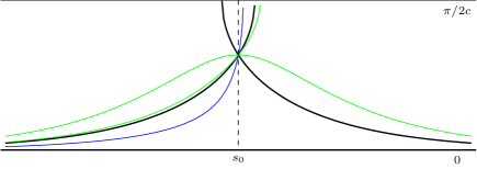
Figure 7. Some generating curves of Grim Reapers of Type II. In black, the light-like solutions. In blue, a time-like solution (Type II.A). In green, a space-like solution with a maximum (Type II.B) and one which blows up to $\pi/2c$ (Type II.C). They have been obtained numerically using Wolfram Mathematica.

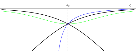
Figure 8. Some generating curves of Grim Reapers of Type III. In black, the light-like solutions. In blue, a time-like solution (Type III.A). In green, a space-like solution (Type III.B). They have been obtained numerically using Wolfram Mathematica.

Declarations

Data availability statement: Data sharing not applicable to this article, as no datasets were generated or analysed during the current study.

Conflict of interest statement: On behalf of all authors, the corresponding author states that there is no conflict of interest.

References

- [1] Luis J. Alías, Alfonso Romero, and Miguel Sánchez. Uniqueness of complete spacelike hypersurfaces of constant mean curvature in generalized Robertson-Walker spacetimes. General Relativity and Gravitation, 27(1):71–84, January 1995.
- [2] Steven J. Altschuler and Lang Wu. Translating surfaces of the non-parametric mean curvature flow with prescribed contact angle. Calculus of Variations and Partial Differential Equations, 2:101–111, 1994.
- [3] Arthur L. Besse. Einstein Manifolds and Topology. Springer Berlin Heidelberg, Berlin, Heidelberg, 1987.
- [4] Carlo Alberto Mantica and Luca Guido Molinari. Generalized Robertson-Walker spacetimes – A survey. International Journal of Geometric Methods in Modern Physics, 14, 2017.
- [5] Qun Chen and Hongbing Qiu. Rigidity of self-shrinkers and translating solitons of mean curvature flows. Advances in Mathematics, 294:517–531, 2016.
- [6] Julie Clutterbuck, Oliver Schnürer, and Felix Schulze. Stability of translating solutions to mean curvature flow. Calculus of Variations and Partial Differential Equations, 29, 10 2005.
- [7] Julie Clutterbuck, Oliver C. Schnürer, and Felix Schulze. Stability of Translating Solutions to Mean Curvature Flow, 2005.
- [8] Henrique Fernandes de Lima. A Note on Maximal Hypersurfaces in a Generalized Robertson-Walker Spacetime. Communications of the Korean Mathematical Society, 37:893–904, 2022.
- [9] Jorge H. S. de Lira and Francisco Martín. Translating solitons in Riemannian products. J. Diff. Equations, 266(12):7780–7812, 2019.
- [10] Jorge H. S. de Lira and Fernanda Roing. Mean curvature flow of graphs in Generalized Robertson-Walker spacetimes with perpendicular Neumann boundary condition. 2022.
- [11] Qiang Guang. Self-shrinkers and translating solitons of mean curvature flow. PhD thesis, 01 2016.
- [12] Richard S. Hamilton. Harnack estimate for the mean curvature flow. Journal of Differential Geometry, 41:215–226, 1995.
- [13] David Hoffman, Tom Ilmanen, Francisco Martín, and Brian White. Notes on translating solitons for mean curvature flow. In Tim Hoffmann, Martin Kilian, Katrin Leschke, and Francisco Martin, editors, Minimal Surfaces: Integrable Systems and Visualisation, pages 147–168, Cham, 2021. Springer International Publishing.
- [14] Gerhard Huisken. Flow by mean curvature of convex surfaces into spheres. Journal of Differential Geometry, 20(1):237 – 266, 1984.
- [15] T. Ilmanen. Elliptic Regularization and Partial Regularity for Motion by Mean Curvature. American Mathematical Society: Memoirs of the American Mathematical Society. American Mathematical Society, 1994.
- [16] Marie-Amélie Lawn and Miguel Ortega. Translating solitons from semi-riemannian foliations, 2016.
- [17] Marie-Amélie Lawn and Miguel Ortega. A fundamental theorem for hypersurfaces in semi-Riemannian warped products. Journal of Geometry and Physics, 90, 2015.
- [18] Marie-Amélie Lawn and Miguel Ortega. Translating Solitons in a Lorentzian Setting, Submersions and Cohomogeneity One Actions. Mediterranean Journal of Mathematics, 19, 06 2022.
- [19] Francisco Martín, Jesús Pérez-García, Andreas Savas-Halilaj, and Knut Smoczyk. A characterization of the grim reaper cylinder. Journal für die reine und angewandte Mathematik (Crelles Journal), 2019(746):209–234, 2019.
- [20] Francisco Martín, Andreas Savas-Halilaj, and Knut Smoczyk. On the topology of translating solitons of the mean curvature flow. Calculus of Variations, 07 2015.
- [21] A.L. Martínez-Triviño and J.P. dos Santos. Uniqueness of the -catenary cylinders by their asymptotic behaviour. Journal of Mathematical Analysis and Applications, 514(2):126347, 2022.
- [22] B. V. O’Neill. The fundamental equations of a submersion. Michigan Mathematical Journal, 13:459–469, 1966.
- [23] B. V. O’Neill. Elementary Differential Geometry. Academic Press, 1997.
- [24] Joel Spruck and Ling Xiao. Complete translating solitons to the mean curvature flow in with nonnegative mean curvature. American Journal of Mathematics, 142, 03 2017.
- [25] Xu-Jia Wang. Convex solutions to the mean curvature flow. Annals of Mathematics, 173(3):1185–1239, 2011.