Investigating nonlinearity in wall turbulence: regenerative versus parametric mechanisms

Both linear growth processes associated with non-normality of the mean flow and nonlinear interaction transferring energy among fluctuations contribute to maintaining turbulence. However, a detailed understanding of the mechanism by which they cooperate in sustaining the turbulent state is lacking. In this report, we examine the role of fluctuation-fluctuation nonlinearity by varying the magnitude of the associated term in the dynamics of Couette flow turbulence to determine how this nonlinear component helps maintain and determine the structure of the turbulent state, and particularly whether this mechanism is parametric or regenerative. Having determined that the mechanism supporting the fluctuation field in Navier-Stokes turbulence is parametric, we then study the mechanism by which the fluctuation component of turbulence is maintained by parametric growth in a time-dependent mean flow by examining the parametric growth mechanism in the frequency domain using analysis of the time-dependent resolvent.

 

1 Distinguishing turbulence regimes: regenerative versus parametric

Turbulence regimes can be distinguished by how nonlinearity participates in maintaining the turbulent state. In this section we describe a study that distinguishes between the parametric and regenerative regimes by performing simulations in which the strength of the fluctuation nonlinearity is varied.

Consider a time-dependent incompressible flow in a parallel channel, comprising the streamwise constant flow, $\mathbf{U}(y,z,t)\equiv(U,V,W)$, and the streamwise varying flow,
$\mathbf{u}^{\prime}(x,y,z,t)\equiv(u^{\prime},v^{\prime},w^{\prime})$. Here, $U$ and $u^{\prime}$ are the velocity components in the streamwise direction $x$, $V$ and $v^{\prime}$ are the velocity components in the cross-stream direction $y$, and $W$, $w^{\prime}$ are the velocity components in the spanwise direction $z$, that evolve according to the equations

$$\partial_{t}\mathbf{U}+{\mathbf{U}\boldsymbol{\cdot}\boldsymbol{\nabla}\mathbf{U}}+\boldsymbol{\nabla}P-\Delta\mathbf{U}/R= {-\langle\mathbf{u}^{\prime}\boldsymbol{\cdot}\boldsymbol{\nabla}\mathbf{u}^{\prime}\rangle_{x}},$$ (1a)

$$\partial_{t}\mathbf{u}^{\prime}+{\mathbf{U}\boldsymbol{\cdot}\boldsymbol{\nabla}\mathbf{u}^{\prime}+\mathbf{u}^{\prime}\boldsymbol{\cdot}\boldsymbol{\nabla}\mathbf{U}}+\boldsymbol{\nabla}p^{\prime}-\Delta\mathbf{u}^{\prime}/R= -\alpha\left(\mathbf{u}^{\prime}\boldsymbol{\cdot}\boldsymbol{\nabla}\mathbf{u}^{\prime}-\langle\mathbf{u}^{\prime}\boldsymbol{\cdot}\boldsymbol{\nabla}\mathbf{u}^{\prime}\rangle_{x}\right),$$ (1b)

$$\boldsymbol{\nabla}\boldsymbol{\cdot}\mathbf{U}=0,\ \ \ \boldsymbol{\nabla}\boldsymbol{\cdot}\mathbf{u}^{\prime}=0,$$ (1c)

with no-slip boundary conditions at the channel walls and periodic boundary conditions in $x$ and $z$. In these equations, the streamwise mean component of a flow field is denoted by $\langle\cdot\rangle_{x}$, and $\alpha$ has been included to allow variation in the influence of the the non-linear interaction among the $\mathbf{u}^{\prime}$ flow components. The pressure fields, $P(y,z,t)$ and $p^{\prime}(x,y,z,t)$, are determined from the incompressibility conditions, and $R$ is a Reynolds number. In this report, we study the turbulence that develops in this system as a function of the parameter $\alpha$. When $\alpha=1$, these equations are the Navier-Stokes equations for the evolution of the total flow $\mathbf{u}=\mathbf{U}+\mathbf{u}^{\prime}$, partitioned into the two flow fields $\mathbf{U}$ and $\mathbf{u}^{\prime}$ corresponding to the streamwise mean component of $\mathbf{u}$ and fluctuations of $\mathbf{u}$ from the streamwise mean. Because of this identification, we refer to $\mathbf{U}$ as the mean and $\mathbf{u}^{\prime}$ as the fluctuations for all values of $\alpha$.

Nonlinearity does not act as an energy source in equations (1) for any value of $\alpha$, and in the absence of dissipation the energy of the total flow, $\int_{V}d^{3}\mathbf{x}~{}|\mathbf{U}+\mathbf{u}^{\prime}|^{2}$, is conserved for all values of $\alpha$. Also, the fluctuation-fluctuation nonlinearity does not contribute to the total energy of the fluctuation field, $\mathbf{u}^{\prime}$, as $\int_{V}d^{3}\mathbf{x}~{}\mathbf{u}^{\prime}\boldsymbol{\cdot}\left(\mathbf{u}^{\prime}\boldsymbol{\cdot}\boldsymbol{\nabla}\mathbf{u}^{\prime}-\langle\mathbf{u}^{\prime}\boldsymbol{\cdot}\boldsymbol{\nabla}\mathbf{u}^{\prime}\rangle_{x}\right)=0$; therefore, a non-vanishing fluctuation field is sustained only by energy transferred between the mean $\mathbf{U}$ and the fluctuations $\mathbf{u}^{\prime}$. This energy transfer arises from transient growth due to non-normality of the mean $\mathbf{U}$. The fluctuation-fluctuation nonlinearity, although it does not make a net contribution to the fluctuation energy, can play a causal role in sustaining the turbulence by redistributing energy among the various fluctuation structures, specifically by replenishing the subset of fluctuations that participate in the non-normality induced transfer of energy from the mean $\mathbf{U}$. We restrict the term regenerative mechanism to refer only to mechanisms in which this feedback from fluctuation-fluctuation nonlinearity in the fluctuation equation is essential to maintaining the fluctuation variance. It has recently been shown that this regenerative mechanism can sustain a non-vanishing fluctuation field in the Navier-Stokes equations (1b) with $\alpha=1$ when the fluctuations interact with a specified time-independent, hydrodynamically stable, wall-bounded mean velocity profile $\mathbf{U}(y,z)$, taken from a sufficiently non-normal streamwise mean flow snapshot from a direct numerical simulation (DNS) (Lozano-Durán et al. 2021).

When $\alpha=0$, this regenerative mechanism is not available to sustain turbulence. Nevertheless, not only is turbulence sustained but also the turbulence that develops, referred to as RNL turbulence, has realistic structure, akin to the corresponding turbulence with $\alpha=1$, even at large Reynolds numbers (Thomas et al. 2014; Bretheim et al. 2015; Farrell et al. 2016, 2017a). This RNL turbulence sustains its fluctuations by non-normal interaction with the time-dependent mean. This mechanism, which underlies the sensitive dependence on initial conditions associated with positive Lyapunov exponents, and the universal exponential growth mechanism of perturbations in random matrix theory identified by Oseledets (1968), will be referred to as the parametric mechanism. Key to the maintenance of the fluctuations by the parametric mechanism is the time dependence of the mean flow, which results in the subspace of the growing fluctuations being continuously replenished in the absence of feedback regeneration by fluctuation-fluctuation nonlinearity.

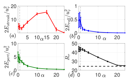
(I)

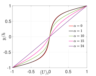
(II)

Figure 1: (I) Time-averaged energies and 1 standard deviation fluctuations (indicated with bars) of (a) the streak, (b) the roll, and (c) the fluctuations obtained from equations (1a)-(1b) for different values of $\alpha$. (d) Time-averaged friction Reynolds number, $R_{\tau}$, for the respective cases; the dashed line indicates its laminar value $\sqrt{R}$. The vertical dashed lines indicate Navier-Stokes turbulence at $\alpha=1$. (II) Time-averaged streamwise mean flow for various values of $\alpha$. For $\alpha>20$, the flow is laminar.

Having identified at $\alpha=0$ a turbulent regime that is maintained exclusively by the parametric mechanism, we wish to examine the mechanism sustaining turbulence as $\alpha$ increases to determine whether turbulence can also be sustained exclusively by feedback regeneration for some value of $\alpha$. Also, we wish to determine whether the principal support of Navier-Stokes turbulence at $\alpha=1$ is the parametric or the feedback regenerative mechanism.

We examine the turbulence that develops as a function of $\alpha$ in DNS in the case of a Couette channel flow at $R=600$ and consider the dependence on $\alpha$ of the friction Reynolds number, $R_{\tau}$; dependence on $\alpha$ of the energy of the streak component of the flow, defined as $E_{s}(t)=\int_{V}d^{3}\mathbf{x}~{}(U-\big{\langle}U\big{\rangle}_{z})^{2}$, with $\big{\langle}U\big{\rangle}_{z}$ denoting the spanwise averaged of the $U$ velocity; dependence on $\alpha$ of the energy of the roll component of the flow, $E_{r}(t)=\int_{V}d^{3}\mathbf{x}~{}(V^{2}+W^{2})$; and also dependence on $\alpha$ of the energy of the fluctuations, $E_{p}=\int_{V}d^{3}\mathbf{x}~{}|\mathbf{u}^{\prime}|^{2}$. In Navier-Stokes turbulence ($\alpha=1$) these flow components underlie the self-sustaining cycle (SSP), which is central to the maintenance of wall turbulence (Hamilton et al. 1995), and are used as diagnostics of the turbulent regime as $\alpha$ varies.

Three fluctuation turbulence regimes can be distinguished using these diagnostics, as shown in Figure 1. The first regime extends from $\alpha=0$ to about $\alpha=2.5$ and in this regime the frictional Reynolds number together with diagnostics of streak, roll, and fluctuation variance, are found to be typical of Navier-Stokes turbulence. Within this regime lies Navier-Stokes turbulence at $\alpha=1$, as well as RNL turbulence at $\alpha=0$. Time-mean streamwise velocity profiles maintained in this Navier-Stokes turbulence regime are nearly indistinguishable, as are the time-dependent streamwise mean turbulent states, streak snapshots of which are shown in Figure 2(a,b). We conclude that the parametric turbulence regime that has been identified to necessarily support RNL turbulence at $\alpha=0$ continues to provide the dynamical mechanism supporting turbulence for all values of $\alpha<2.5$, including Navier-Stokes turbulence at $\alpha=1$. This turbulent regime can be identified with the time-dependent SSP described in Hamilton et al. 1995. As $\alpha$ is increased above $\alpha\approx 2.5$, the character of the turbulence changes, with a secular increase in the streak amplitude together with a decrease in the roll and perturbation amplitude (Figures 1(Ia,b,c)). This progression marks the transition toward a state of turbulence that is sustained by an almost constant time mean flow and, therefore, with fluctuations that are sustained exclusively by the feedback regenerative mechanism in the absence of an SPP cycle. This feedback regenerative turbulence state corresponds to an analytic fixed point of the dynamics of the cumulants of the flow closed at second order (S3T) (Farrell & Ioannou 2012; Farrell et al. 2017b). Figure 2(c) shows an example of this fixed-point state at $\alpha=10$. This state is similar to that obtained by Lozano-Durán et al. 2021, with the important distinguishing characteristic that this state is self-maintaining. We conclude that the parametric regime is required for the maintenance of RNL and Navier-Stokes turbulence but that a turbulent state is also maintained for $\alpha>2.5$, indicating that maintaining turbulence by the feedback regenerative mechanism is possible. As $\alpha$ is increased further beyond values supporting the fixed-point regenerative turbulence, the turbulence eventually laminarizes, as indicated by the approach of the frictional Reynolds number and mean flow diagnostics to laminar values (Figures 1(Id),(II)). We note that as $\alpha$ increases, the spatial spectrum of the turbulence flattens, and it becomes impossible to prevent backscatter to the larger scales from the smallest scales retained in the DNS. For this reason, as shown in Figure 1(Ic), there remains a small level of fluctuations at $\alpha>15$ in what we believe should have been a strictly laminar state. Corroboration is provided by the fact that S3T at these values of $\alpha$, with a stochastic parameterization of the fluctuation-fluctuation nonlinearity in which backscatter is not supported, do obtain the laminar state.

We conclude that the regime of turbulence that includes RNL and Navier-Stokes turbulence is maintained by the parametric mechanism of energy transfer from the mean to the fluctuation field that is isolated using RNL analysis. This parametric turbulence regime does not depend on fluctuation-fluctuation nonlinearity for its support. With the fluctuation-fluctuation nonlinearity shown to be unnecessary for the maintenance of the fluctuation component of turbulence, we turn our attention to the remaining nonlinearity, which is the parametric transfer of energy from the time-dependent mean flow to the fluctuation field. This transfer is associated with the Lyapunov vectors of the time-dependent mean flow.

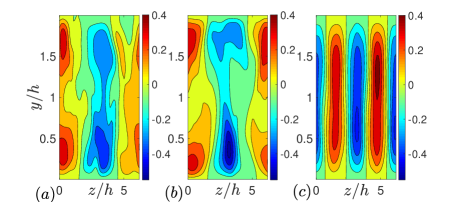
Figure 2: Snapshots of the streak. (a) in RNL turbulence for $\alpha=0$, (b) in Navier-Stokes turbulence, $\alpha=1$, and (c) in the almost stationary state of turbulence at $\alpha=10$.           

2 Resolvent analysis of time-dependent systems

We continue our study of the role of nonlinearity in turbulence by studying the mechanism by which fluctuations are amplified by non-normal interaction with a time-dependent mean flow. Our analysis method is performed in the frequency domain and is based on extension of resolvent analysis to time-dependent mean flows. The formalism presented builds on that presented by Wereley(1991), Fardad et al. (2008), Padovan et al. (2020), Rigas et al. (2021), and Franceschini et al. (2022). We begin by recalling that turbulence in shear flow is sustained by transfer of energy from the large-spatial-scale externally forced flow field to the small-scale fluctuation field and that this transfer is mediated by the non-normality of the large-scale forced flow. Non-normal interaction between large- and small-scale components of the turbulent flow field can be analyzed in either the time or frequency domain, and both of these approaches are contained within generalized stability theory (GST) (Farrell & Ioannou, 1996a, b, 1999; Schmid & Henningson, 2001). However, while transient growth analysis for time-dependent flows is well developed in the time domain, analysis of the GST of time-dependent flows in the frequency domain is less developed. This is important because the large-scale streamwise mean flows involved in the dynamics of shear turbulence are highly time-dependent. Moreover, as we have seen, the fluctuation component of the turbulence is maintained by parametric growth, which motivates a closer analysis of the mechanism by which parametric growth takes place.

The dynamics of perturbations, $x$, linearized about a time-dependent mean state can be written, using a partition into the time-mean, $A$, and perturbation, $B$, operators, as

$$\dot{x}=(A+B(t))x+f(t),$$ (2)

where $f(t)$ is a time-dependent excitation. Assuming asymptotic stability of the system, by Fourier transforming Eq. (2), we obtain

$$-i\omega\hat{x}(\omega)=A\hat{x}(\omega)+\frac{1}{\sqrt{2\pi}}\int_{-\infty}^{\infty}d\omega^{\prime}~{}\widehat{B}(\omega-\omega^{\prime})\hat{x}(\omega^{\prime})+\hat{f}(\omega),$$ (3)

where $\hat{x}(\omega)$ is the Fourier transform of the state $x(t)$ and $\widehat{B}(\omega)$ the transform of the operator $B(t)$. Because of the convolution in Eq. (3) the temporal evolution of individual free modes of this time-dependent system will not be characterized solely by the eigenvalues of $A$, and the asymptotic response of the system to an excitation at a single frequency will not be restricted to the frequency of the forcing. Analysis of the dynamics in frequency space governed by Eq. (3) proceeds by defining an operator, $H$, acting on all the Fourier components of $\hat{x}$, as

$$\left.H\hat{x}\right|_{\omega}\equiv i\omega\hat{x}(\omega)+A\hat{x}(\omega)+\frac{1}{\sqrt{2\pi}}\int_{-\infty}^{\infty}d\omega^{\prime}~{}B(\omega-\omega^{\prime})\hat{x}(\omega^{\prime}).$$ (4)

We refer to this operator as the Hill operator. The frequency response of the time-dependent dynamics (Eq. (2)) to excitation $f(t)$ is given in terms of the resolvent of the Hill operator, $R=-H^{-1}$, which determines the response, $\hat{x}=R\hat{f}$. The eigenfunctions of $R$, which are also the eigenfunctions of $H$, are the resonant responses of this time-dependent system.

2.1 Physical meaning and properties of the spectrum of the Hill operator

Consider the linear dynamics

$$\dot{x}=(A+B(t))x.$$ (5)

The eigenfunctions of $H$ can be identified with the time development of the covariant Lyapunov vectors (CLVs) of this system and the real part of the eigenvalues of $H$ with the Lyapunov exponents of the corresponding CLVs. As an example consider $B(t)=B\cos t$. In this periodic case, we know from Bloch’s theorem that the eigenfunctions of the dynamics, i.e. the CLVs, are of the form $x_{\lambda}(t)=e^{\lambda t}\chi_{\lambda}(t)$, where $\chi_{\lambda}$ is a periodic function with period $2\pi$, and that the real part of the exponent $\lambda$ is the Lyapunov exponent of this CLV and the imaginary part of $\lambda$ is the mean rate of phase advance of the periodic function $\chi_{\lambda}$. The connection between the eigenfunctions of $H$ and the CLVs of Eq. (5) arises because the periodic function component of the CLV, $\chi_{\lambda}$, is the Fourier transform of the eigenfunction of $H$ with eigenvalue $\lambda$. Indeed, if we write the periodic function $\chi_{\lambda}(t)$ as a Fourier series, $\chi_{\lambda}(t)=\sum_{n=-\infty}^{\infty}\hat{x}_{n}e^{-int}$, the eigenfunction becomes $x_{\lambda}(t)=e^{\lambda t}\sum_{n=-\infty}^{\infty}\hat{x}_{n}e^{-int}$, and upon introducing this functional form in Eq. (5), we find, by matching the corresponding Fourier components that arise in the expansion of Eq. (5), that the Fourier components $\hat{x}_{n}$ must satisfy for all $n$ the recurrence relations

$$in\hat{x}_{n}+A\hat{x}_{n}+\frac{B}{2}\left(\hat{x}_{n+1}+\hat{x}_{n-1}\right)=\lambda\hat{x}_{n}.$$ (6)

The left side of Eq. (6) is the $n$-th Fourier component of $H\hat{x}$, with $H$ the Hill operator discretized on the integer-valued frequency lattice and Eq. (6) is the statement that $\hat{x}$ is the eigenfunction of $H$ with eigenvalue $\lambda$, which we have shown to be equivalent to the statement that the CLV $x_{\lambda}(t)=e^{\lambda t}\chi_{\lambda}(t)$ satisfies Eq. (5). Note also from Eq. (6) that if $\hat{x}_{n}$ are the components of an eigenfunction of $H$ with eigenvalue $\lambda$, then for any integer $m$, $\hat{y}_{n}=\hat{x}_{n-m}$, will also be an eigenfunction of $H$ with eigenvalue $\lambda+im$. However, all these shifted eigenfunctions of $H$ correspond to the same CLV as $x_{\lambda}(t)=e^{\lambda t}\sum_{n=-\infty}^{\infty}\hat{x}_{n}e^{-int}=e^{\lambda t}\sum_{n=-\infty}^{\infty}\hat{x}_{n-m}e^{-i(n-m)t}=e^{(\lambda+im)t}\sum_{n=-\infty}^{\infty}\hat{y}_{n}e^{-int}$. The shifted eigenfunctions of $H$ arise because the periodic function $\chi(t)$, which is associated with the eigenfunction of $H$, can be multiplied by an arbitrary exponential, $e^{imt}$, with the underlying period. All these shifted eigenfunctions are required in order to produce completeness of the representation in the frequency domain.

The above analysis carries over to the general case when $B(t)$ is not periodic. The CLVs of Eq. (5) are then written as $x_{\lambda}(t)=e^{\lambda t}\int_{-\infty}^{\infty}d\omega~{}\hat{x}(\omega)~{}e^{-i\omega t}$, and upon introduction of this expression in Eq. (5), we find that the components of $\hat{x}$ must satisfy

$$\left.H\hat{x}\right|_{\omega}\equiv i\omega\hat{x}(\omega)+A\hat{x}(\omega)+\frac{1}{\sqrt{2\pi}}\int_{-\infty}^{\infty}d\omega^{\prime}~{}B(\omega-\omega^{\prime})\hat{x}(\omega^{\prime})=\lambda\hat{x}(\omega),$$ (7)

in other words that $\hat{x}$ should be an eigenfunction of $H$ with eigenvalue $\lambda$. Also, as in the periodic case, if $\hat{x}_{\lambda}$ is an eigenfunction of $H$ with eigenvalue $\lambda$ so is $\hat{x}_{\lambda,\alpha}(\omega)=\hat{x}_{\lambda}(\omega-\alpha)$ with eigenvalue $\lambda+i\alpha$, obtained by shifting $\hat{x}_{\lambda}$ by $\alpha$, and all these eigenfunctions produce the time evolution of the same CLV, $x_{\lambda}(t)$, in the time domain. Note that Floquet analysis determines the CLV only at a chosen time, while the Hill matrix approach obtains the full time evolution of the CLVs.

2.2 Variance maintained at steady state by stochastic excitation and optimal response to harmonic excitation of the time-dependent dynamics

We want to determine the modification to the steady-state response to stochastic excitation resulting from time dependence of the system dynamics. In the energy metric, this response can be conveniently obtained using the ${\cal L}^{2}$ norm $||\hat{x}||^{2}=\int_{-\infty}^{\infty}d\omega~{}|\hat{x}(\omega)|^{2}$ by first transforming $\hat{x}$ into energy coordinates so that this ${\cal L}^{2}$ norm corresponds to energy. Assuming that the time-dependent operator, $A+B(t)$, is stable, the ensemble mean energy density at steady state is $\delta\omega~{}{\rm trace}\left(\langle\hat{x}\hat{x}^{\dagger}\rangle\right)$, which is $\delta\omega~{}{\rm trace}\left(R\langle\hat{f}\hat{f}^{\dagger}\rangle R^{\dagger}\right)=\delta\omega/(2\pi)~{}{\rm trace}\left(RR^{\dagger}\right)\equiv\delta\omega/(2\pi))||R||_{F}^{2}$, where $||R||_{F}$ is the Frobenius norm of the Hill resolvent and $\delta\omega$ is the increment in frequency of the Riemann sum approximation of the integral in the ${\cal L}^{2}$ norm. We have assumed whiteness of the stochastic excitation, that is, that the spatial components of the forcing satisfy $\langle\hat{f}_{i}(\omega)\hat{f}_{j}^{*}(\omega^{\prime})\rangle=\delta_{ij}\delta_{\omega,\omega^{\prime}}/(2\pi)$. When the dynamics is discretized on a finite grid, $||R||_{F}$ is the square root of the sum of the squares of the singular values of $R$. In the time-independent case it is useful to compare the variance maintained by the system to the variance that would be maintained if the system were normal and therefore the modes of the system were orthogonal and as a consequence contribute to the variance without intermodal interactions. The variance of this equivalent normal system per unit forcing is given by the classical resonant response to forcing, $||R_{eq}||_{F}=\sum_{i}1/(2\lambda_{i})$, where $\lambda_{i}$ are the decay rates of the modes. By necessity $||R_{eq}||_{F}\leq||R||_{F}$ (Ioannou, 1995), and the ratio $||R||_{F}/||R_{eq}||_{F}$ can serve as a measure of the non-normality of the dynamics. In time-dependent dynamics we can similarly define the variance of the effectively normal system, $||R_{eff}||_{F}=\sum_{i}1/(2\lambda_{i})$, where now the $\lambda_{i}$ are the Lyapunov exponents of the time-dependent dynamics. We could also consider $||R(\varepsilon)||_{F}/||R_{eff}(\varepsilon)||_{F}$ as a measure of the mean non-normality of the CLVs.

In addition to the variance, it is of interest to obtain the optimal response that could result from a deterministic harmonic excitation at frequency $\omega_{e}$. This is given by the ${\cal L}^{2}$ norm of $RP_{\omega_{e}}$, where $P_{\omega_{e}}$ is the operator that projects $\hat{f}$ to its value at the excitation frequency $\omega_{e}$. When the dynamics is discretized on a finite grid, it is given by the largest singular value of $RP_{\omega_{e}}$. In the time independent case we can similarly define the equivalent normal response to be the response that obtains when the modes of $A$ are assumed to be orthogonal.

Consider the damped Mathieu equation, which is the prototypical example of parametric instability, with

$$A=\left(\begin{array}[]{ccc}0&1\\ -\omega_{0}^{2}&-2\gamma\end{array}\right),~{}~{}~{}B(t)=\varepsilon\cos(\omega_{f}t)B,~{}~{}B=\left(\begin{array}[]{ccc}0&0\\ 1&0\end{array}\right),$$ (12)

where $\gamma=0.05$, $\omega_{0}=1$, and $\omega_{f}=2$. These parameters correspond to forcing at twice the resonant frequency, which can be shown to lead to maximal amplification. The associated Hill operator becomes

$$\left.H\hat{x}\right|_{\omega}=i\omega\hat{x}(\omega)+A\hat{x}(\omega)+\frac{\varepsilon}{2}B(\hat{x}(\omega-\omega_{f})+\hat{x}(\omega+\omega_{f})),$$ (13)

which in the calculations will be discretized on a finite lattice of frequencies. Figure 3(a) shows the variance maintained under stochastic excitation as a function of $\varepsilon$. As expected, the maintained variance increases as $\varepsilon$ approaches the critical $\varepsilon_{c}$ at which the dynamics become unstable ($\varepsilon_{c}=0.2$ for these parameters). Also shown is the effective non-normality of the dynamics measured by $||R(\varepsilon)||_{F}/||R_{eff}(\varepsilon)||$. At these parameter values, the maintained variance increases at the rate predicted by the inverse sum of the Lyapunov exponents of the two CLVs, as if the CLVs of the Mathieu equation were normal coordinates. This is reflected in the minimal increase of the effective non-normality of the time-dependent dynamics as a function of $\varepsilon$, shown by the dashed line in Figure 3(a). Note also that this figure verifies that the Mathieu equation is normal at $\varepsilon=0$. The variance maintained by excitation of the parametric Mathieu oscillator is also close to the variance of the equivalent normal system at other parameter values. Figure 4(a) shows that the optimal response to harmonic forcing with $\varepsilon=0.18$ and $\varepsilon=0$ is maximized in both cases for forcing at the resonant frequencies $\omega=\pm\omega_{0}$. Also, given that $\omega_{f}=2\omega_{0}$, there is strong response at the sideband frequencies $\omega=\pm 3\omega_{0}$. We conclude that, in the case of the asymptotically stable Mathieu equation, time dependence produces an enhanced response primarily due to a decrease of the decay rate of the Lyapunov exponents of the system.

In contrast to the Mathieu oscillator, which is characterized by normal mean dynamics, the streamwise mean of a shear flow is typically highly non-normal, even when the streamwise mean flow is time-independent. For example, consider the resolvent analysis for plane wave perturbations in a plane parallel channel in $y\in[-1,1]$ with streamwise mean flow $U(y,t)=U_{0}(y)+\varepsilon\cos(\omega_{f}t)U_{1}(y)$, where $U_{0}(y)=1-y^{2}$ and $U_{1}(y)=\sin(2\pi y)$, and with forcing frequency $\omega_{f}=0.3$, streamwise wavenumber $k=1.143$, and spanwise wavenumber $m=1.67$ at Reynolds number $R=800$. The excitation frequencies $\omega_{f}$ have been chosen to lie in the interval for which time dependence leads to an amplified response, which is for frequencies in the range $0.08<\omega_{f}<0.35$. The perturbations evolve according to the Orr-Sommerfeld-Squire (OSS) equations, where $A$ and $B$ are, respectively, the time-independent and time-dependent components of the OSS operator. The complex $A$ and $B$ operators are discretized and expressed in energy coordinates as in Butler & Farrell (1992).

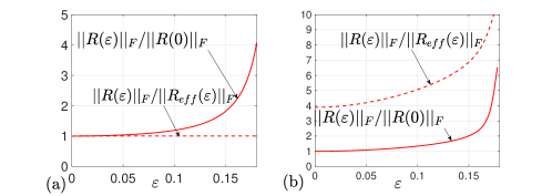
Figure 3: Shown as a function of the amplitude of the time dependence $\varepsilon$ are the root-mean-square variance, $||R||_{F}$, maintained under white stochastic excitation (solid lines), and the ratio of the variance maintained by the time-dependent system to the variance, $||R_{eff}||_{F}$, maintained by the effectively normal dynamics (dashed lines). (a) Results for the Mathieu equation with $\omega_{f}=2\omega_{0}$, $\omega_{0}=1$, and $\gamma=0.05$. The oscillator becomes unstable with these parameters at $\varepsilon_{c}=0.2$. (b) Results for the time-modulated Poiseuille flow at $R=800$ excited with perturbations with wavenumbers $k=1.143$, and $m=1.67$. The time-dependent Poiseuille flow becomes unstable at $\varepsilon_{c}=0.178$.

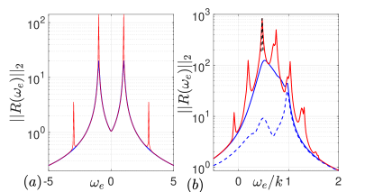
Figure 4: The optimal response $||R(\omega_{e})||_{2}$ as a function of $\omega_{e}$. (a) Results for the Mathieu equation with $\omega_{f}=2\omega_{0}$, $\omega_{0}=1$, and $\gamma=0.05$. The blue line is the response for $\varepsilon=0$, and the red line is the response for $\varepsilon=0.18$. (b) Results for the time-modulated Poiseuille flow. The solid blue line represents the response without time dependence ($\varepsilon=0$), the dashed blue line represents the equivalent normal response, $||R_{eq}||_{2}$, of the time-independent $A$ operator. The red line represents the response with time dependence ($\varepsilon=0.16$ and $\omega_{f}=0.3$). The peaks are separated by $\omega_{f}$ and their width is determined by the Lorentzian (dashed black curve) corresponding to the Lyapunov exponent.

Figure 3(b) shows the maintained variance and the effective mean non-normality of the time-dependent dynamics as a function of $\varepsilon$ for the case of $\omega_{f}=0.3$. Unlike in the case of the parametric oscillator, both the variance and the effective mean non-normality increase with the amplitude of the time-dependent component of the dynamics. Figure 4(b) shows the optimal response as a function of excitation frequency. The response is asymmetric with respect to the zero frequency as $A$ and $B$ are complex matrices and has substantial amplitude for $\omega_{e}/k$ within the range of the speeds of the mean flow. The response of the time-dependent system is highly amplified at the frequency of the largest non-normal response of the time-independent operator, which is at $\omega_{e}/k\approx 0.48$; and in sideband frequencies that are separated from the frequency of the main maximum peak by integral multiples of $\omega_{f}$. The equivalent-normal response (dashed blue line in Figure 4(b)) peaks at $\omega_{e}/k\approx 1$, which corresponds to the frequency of the least damped mode of $A$, while the variance of the time-dependent dynamics peaks at $\omega_{e}/k=0.48$, which corresponds to the frequency of maximum non-normality of the time-independent operator, indicating that it is the non-normal structures of the time-independent dynamics that primarily influences both the time-independent and the time-dependent response. Also note that, the response peaks irrespectively of the frequency of the time modulation, $\omega_{f}$, at frequency $\omega_{e}/k\approx 0.48$ and not at twice the frequency, as was the case in the effectively normal Mathieu oscillator. The largest Lyapunov exponent of the flow also determines the width of the Lorentzian peaks of the time-dependent response, as shown in Figure 4(b).

3 Conclusions

This report describes a study of the interaction among linear non-normal growth, fluctuation-fluctuation nonlinearity, and time dependence of the streamwise mean flow in the dynamics of turbulence in shear flow. In the first part of this study an experiment is described in which the nonlinear fluctuation-fluctuation term in a streamwise mean and fluctuation from the streamwise mean partition of the Navier-Stokes equations are modified to allow variation in the magnitude of the fluctuation-fluctuation nonlinearity by a factor $\alpha$. Three turbulent regimes were found as $\alpha$ was varied: a parametric regime that includes RNL turbulence at $\alpha=0$ and Navier-Stokes turbulence at $\alpha=1$; transition to a feedback regenerative regime with a constant streamwise mean flow at $\alpha\approx 10$, and finally a laminar regime for $\alpha>20$. Having identified the parametric regime as supporting the turbulent state in Navier-Stokes and RNL turbulence, we turned in the second part of this study to an examination of the mechanism of parametric growth using time-dependent resolvent analysis. The non-normality of the mean operator and, in particular, the frequency of maximum optimal response of the time-independent operator were found to determine the central and sideband frequencies of the time-dependent system and the structure of the optimal response to harmonic excitation. Also, the non-normal growth mechanism was found using Hill matrix analysis to be partitioned in a system-dependent manner between contributions from the non-normality of the mean and that of the time-dependent components of the operator (as in Fig 3).

Unlike the cases treated in this report, time variations of the mean flow in turbulence are broadband in frequency. From our results, we expect that time dependence will amplify primarily the highly non-normal structures of the time-independent flow, so that while with broadband mean flow time dependence the response will be smoother than the response that arises when the fluctuations of the mean flow are confined to distinct frequencies, it will still be characterized primarily by the structure of the most amplified structure of the time-independent dynamics.

Acknowledgments

We thank Prof. Georgios Rigas, Prof. Adrian Lozano-Durán, Prof. Javier Jiménez and Dr. Mario di Renzo for their useful comments and discussions.

References

- Bretheim et al. (2015) Bretheim, J. U., Meneveau, C. & Gayme, D. F. 2015 Standard logarithmic mean velocity distribution in a band-limited restricted nonlinear model of turbulent flow in a half-channel. Phys. Fluids 27, 011702.
- Butler & Farrell (1992) Butler, K. M. & Farrell, B. F. 1992 Three-dimensional optimal perturbations in viscous shear flows. Phys. Fluids 4, 1637–1650.
- Fardad et al. (2008) Fardad, M., Jovanovic, M. R. & Bamieh, B. 2008 Frequency analysis and norms of distributed spatially periodic systems. IEEE Transactions on Automatic Control 53, 2266–2279.
- Farrell et al. (2017a) Farrell, B. F., Gayme, D. F. & Ioannou, P. J. 2017a A statistical state dynamics approach to wall-turbulence. Phil. Trans. R. Soc. A 375 (2089), 20160081.
- Farrell & Ioannou (1996a) Farrell, B. F. & Ioannou, P. J. 1996a Generalized stability theory. Part I: Autonomous operators. J. Atmos. Sci. 53, 2025–2040.
- Farrell & Ioannou (1996b) Farrell, B. F. & Ioannou, P. J. 1996b Generalized stability theory. Part II: Non-autonomous operators. J. Atmos. Sci. 53, 2041–2053.
- Farrell & Ioannou (1999) Farrell, B. F. & Ioannou, P. J. 1999 Perturbation growth and structure in time dependent flows. J. Atmos. Sci. 56, 3622–3639.
- Farrell & Ioannou (2012) Farrell, B. F. & Ioannou, P. J. 2012 Dynamics of streamwise rolls and streaks in turbulent wall-bounded shear flow. J. Fluid Mech. 708, 149–196.
- Farrell et al. (2016) Farrell, B. F., Ioannou, P. J., Jiménez, J., Constantinou, N. C., Lozano-Durán, A. & Nikolaidis, M.-A. 2016 A statistical state dynamics-based study of the structure and mechanism of large-scale motions in plane Poiseuille flow. J. Fluid Mech. 809, 290–315.
- Farrell et al. (2017b) Farrell, B. F., Ioannou, P. J. & Nikolaidis, M.-A. 2017b Instability of the roll–streak structure induced by background turbulence in pre-transitional Couette flow. Phys. Rev. Fluids 2, 034607.
- Franceschini et al. (2022) Franceschini, L., Sipp, D., Marquet, O., Moulin, J. & Dandois, J. 2022 Identification and reconstruction of high-frequency fluctuations evolving on a low-frequency periodic limit cycle: application to turbulent cylinder flow. Journal of Fluid Mechanics 942, A28.
- Hamilton et al. (1995) Hamilton, J. M., Kim, J. & Waleffe, F. 1995 Regeneration mechanisms of near-wall turbulence structures. Journal of Fluid Mechanics 287, 317–348.
- Ioannou (1995) Ioannou, P. J. 1995 Non-normality increases variance. J. Atmos. Sci. 52, 1155–1158.
- Lozano-Durán et al. (2021) Lozano-Durán, A., Constantinou, N. C., Nikolaidis, M.-A. & Karp, M. 2021 Cause-and-effect of linear mechanisms sustaining wall turbulence. Journal of Fluid Mechanics 914, A8.
- Oseledets (1968) Oseledets, V. I. 1968 A multiplicative ergodic theorem. Lyapunov characteristic numbers for dynamical systems. Trans. Moscow Math. Soc. 19, 197–231.
- Padovan et al. (2020) Padovan, A., Otto, S. E. & Rowley, C. W. 2020 Analysis of amplification mechanisms and cross-frequency interactions in nonlinear flows via the harmonic resolvent. Journal of Fluid Mechanics 900, A14.
- Rigas et al. (2021) Rigas, G., Sipp, D. & Colonius, T. 2021 Nonlinear input/output analysis: application to boundary layer transition. Journal of Fluid Mechanics 911, A15.
- Schmid & Henningson (2001) Schmid, P. J. & Henningson, D. S. 2001 Stability and Transition in Shear Flows. Springer, New York.
- Thomas et al. (2014) Thomas, V., Lieu, B. K., Jovanović, M. R., Farrell, B. F., Ioannou, P. J. & Gayme, D. F. 2014 Self-sustaining turbulence in a restricted nonlinear model of plane Couette flow. Phys. Fluids 26, 105112.
- Wereley (1991) Wereley, N. M. 1991 Analysis and control of linear periodically time varying systems. PhD thesis, Massachusetts Institute of Technology, Cambridge, U.S.A.