Learning Single Image Defocus Deblurring with Misaligned Training Pairs

Abstract

By adopting popular pixel-wise loss, existing methods for defocus deblurring heavily rely on well aligned training image pairs. Although training pairs of ground-truth and blurry images are carefully collected, e.g., DPDD dataset, misalignment is inevitable between training pairs, making existing methods possibly suffer from deformation artifacts. In this paper, we propose a joint deblurring and reblurring learning (JDRL) framework for single image defocus deblurring with misaligned training pairs. Generally, JDRL consists of a deblurring module and a spatially invariant reblurring module, by which deblurred result can be adaptively supervised by ground-truth image to recover sharp textures while maintaining spatial consistency with the blurry image. First, in the deblurring module, a bi-directional optical flow-based deformation is introduced to tolerate spatial misalignment between deblurred and ground-truth images. Second, in the reblurring module, deblurred result is reblurred to be spatially aligned with blurry image, by predicting a set of isotropic blur kernels and weighting maps. Moreover, we establish a new single image defocus deblurring (SDD) dataset, further validating our JDRL and also benefiting future research. Our JDRL can be applied to boost defocus deblurring networks in terms of both quantitative metrics and visual quality on DPDD, RealDOF and our SDD datasets.

Introduction

Defocus blur occurs when the Depth of Field (DoF) of a camera is not enough to cover the whole captured scene. Although having potential benefits in photography aesthetics, defocus blur degrades visual quality of images, thereby bringing difficulty for downstream tasks like object detection (Kong et al. 2020; Zheng et al. 2022) and tracking (Sun et al. 2022). Defocus deblurring is a challenging task due to spatially variant blur kernels. According to the input data type, existing defocus deblurring methods can be categorized into single image defocus deblurring and dual-pixel defocus deblurring. Compared with dual-pixel defocus deblurring (Abuolaim and Brown 2020; Pan et al. 2021; Abuolaim et al. 2021; Xin et al. 2021) that requires specialized hardware (Śliwiński and Wachel 2013; Herrmann et al. 2020), single image defocus deblurring is a more general yet challenging task, which is the focus of this work. A typical solution to single image defocus deblurring is to estimate a defocus blur map at first, and then non-blind deconvolution (Krishnan and Fergus 2009; Fish et al. 1995) can be adopted to predict the latent sharp image (Shi, Xu, and Jia 2015; Yi and Eramian 2016; DAndrs et al. 2016; Karaali and Jung 2017; Lee et al. 2019; Park et al. 2017). However, methods in this line yield unsatisfactory performance in real-world scenes due to inaccurate estimation of defocus maps.

Recently, deep learning has boosted the performance of defocus deblurring methods (Abuolaim and Brown 2020; Son et al. 2021; Lee et al. 2021), making the acquirement of abundant training data an urgent need.

\begin{overpic}[width=237.7689pt]{figs/intro} \put(-4.5,20.0){$\bm{I}_{B}$} \put(-4.5,7.0){$\bm{I}_{S}$} \put(36.7,7.0){$\bm{I}_{S}$} \put(36.5,20.0){$\bm{I}_{B}$} \par\put(13.0,-3.0){(a) DPDD} \put(59.0,-3.0){(b) RealDOF} \end{overpic}

Figure 1: Misaligned image pairs of ground-truth $\bm{I}_{S}$ and blurry $\bm{I}_{B}$ in DPDD and RealDOF datasets. Although ground-truth and blurry image pairs in these datasets are designed to be aligned, slight misalignment still exists.

A common choice for expanding training sources is data synthesis, yet the domain gap between real-world scenes and synthesized ones makes it inappropriate for training defocus deblurring networks. Currently, DPDD (Abuolaim and Brown 2020) is the most popular real-world defocus deblurring dataset. Although originally targeted at dual-pixel defocus deblurring, DPDD also provides pairwise blurry and sharp images, thus benchmarking single image defocus deblurring. In DPDD dataset, training pairs are intended to be well aligned by adjusting camera aperture via remote control signal. However, misalignment between blurry and sharp images are still inevitable as shown in Fig. 1. In another testing dataset RealDOF (Lee et al. 2021), a dual-camera system is established to capture image pairs, but spatial misalignment can still be observed. By adopting pixel-wise loss, e.g., MSE or $\ell_{1}$-norm, spatial deformation is also learned by deblurrinlg network, possibly yielding deformation artifacts in deblurred image, as shown in Fig. 8.

In this work, we propose a joint deblurring and reblurring learning (JDRL) framework for better exploiting misaligned data as well as a new dataset SDD for single image defocus deblurring. As shown in Fig. 2, JDRL consists of a deblurring module with adaptive deblurring loss and a spatially invariant reblurring module. First, in deblurring module, we introduce optical flow-based deformation to tolerate misalignment between deblurred result and ground-truth sharp image, and then pixel-wise loss can be imposed to recover sharp textures in deblurred image. To tackle the possible inaccurate deformation, we introduce a calibration mask and cycle deformation. Second, in reblurring module, we suggest that the deblurred result should be spatially consistent with the blurry image. To this end, we propose a reblurring network to generate a blurred image, where isotropic blur kernels are predicted to guarantee the spatial invariance between deblurred, reblurred and blurry images. By adopting JDRL, deblurring networks can learn to adaptively exploit sharp textures from ground-truth image, while keeping spatial consistency with input. JDRL is not coupled with the network architecture, and thus it can be applied to enhance existing deblurring methods.

Moveover, a new dataset SDD with high resolution and diverse contents is established for single image defocus deblurring, where a HUAWEI X2381-VG camera is employed to collect blurry and sharp image pairs by adjusting camera motor or aperture size. When collecting SDD dataset, we also try to keep alignment between training pairs, but misalignment still exists due to the consumer camera and collecting settings. There are two types of misalignment: zoom misalignment and shift misalignment (Fig. 5). The misalignment in SDD is generally much intenser than DPDD, making it both a good testing bed for JDRL and a benchmark to benefit future research.

Extensive experiments on DPDD and SDD datasets indicate that JDRL can boost the performance of existing methods. Especially on SDD dataset, the adverse effects of severe misalignment can be significantly relieved by JDRL. When tested on RealDoF dataset, our method also reveals better generalization ability. In summary, the contributions of this paper are three-fold:

• A joint deblurring and reblurring learning framework is proposed for better exploiting misaligned training pairs in training single image defocus deblurring networks.

• A novel reblurring module is proposed to reconstruct reblurred defocus image, where isotropic blur kernels are predicted to keep the spatial consistency between deblurred result and input blurry image.

• A new dataset SDD with high resolution image pairs and diverse contents is established for single image defocus deblurring, benefiting future research in this field.

Related Work

Defocus Deblurring Methods

A popular paradigm for single image defocus deblurring is first estimating a defocus map and then adopting non-blind deconvolution (Krishnan and Fergus 2009; Fish et al. 1995) to predict the sharp image  (Shi, Xu, and Jia 2015; Yi and Eramian 2016; DAndrs et al. 2016; Karaali and Jung 2017; Lee et al. 2019; Park et al. 2017). However, methods of this kind not only lead to excessive time consumption, but also yield unsatistactory performance due to inaccurately estimated defocus maps and over idealized blur kernel models.

Recent methods mostly employ deep learning networks to ameliorate the defects of traditional methods (Abuolaim and Brown 2020; Son et al. 2021; Lee et al. 2021). Abuolaim et al. (Abuolaim and Brown 2020) proposed the first deep learning based model to perform defocus deblurring and released the DPDD dataset. IFAN (Lee et al. 2021) proposed an iterative filter adaptive network, which is trained with an extra reblur loss. Son et al. (Son et al. 2021) introduced a framework with a kernel-sharing parallel atrous convolution block for defocus deblurring. DRBNet (Ruan et al. 2022) adopts an extra light field dataset in the training stage, which considerably improves the network performance. In spite of decent performance, existing methods are limited to the vanilla training framework using pixel-wise loss, which can not handle the misalignment between training image pairs. In comparison, this paper firstly takes into account the issue of misalignment tolerance, and establishes the JDRL framework to improve the network performance without using extra datasets.

Defocus Deblurring Datasets

The performance of CNN-based methods is largely dependent on the training data. Nevertheless, it can be a labor-intensive project to establish a well qualified defocus deblurring dataset. Although there exist several blur-related datasets, i.e., CUHK (Shi, Xu, and Jia 2014), DUT (Zhao et al. 2018), SYNDOF (Lee et al. 2019), MC-blur (Zhang et al. 2022), LFDOF (Ruan et al. 2022) and RealDOF (Lee et al. 2021) dataset, most of them are mainly built for network testing (Lee et al. 2021) or blur detection (Cun and Pun 2020; Tang et al. 2019). DPDD is the only widely adopted real-world training dataset. A premise of DPDD is the alignment between blurry-sharp image pairs. In this regard, the adjustment of camera aperture size is conducted by a remote signal control to avoid human interference. However, since the image pairs are not captured simultaneously, slight misalignment can inevitably arise. Lee et al. (Lee et al. 2021) built the RealDOF dataset using a dual-camera system, which can concurrently capture the blurry and sharp images. Following (Rim et al. 2020), a post-processing stage is also adopted to deal with the misalignment. However, as shown in Fig. 1, there still exists misalignment in RealDOF. In this paper, instead of endeavoring to build a perfectly aligned dataset, we propose to (i) make possible the easy acquirement of training data by relaxing the constraint of pairwise alignment and (ii) improve the results of defocus deblurring on existing datasets by taking misalignment into account. Additionally, we propose a new dataset named SDD to validate the effectiveness of our JDRL framework.

Proposed Method

In this section, we first introduce the pipeline of joint deblurring and reblurring learning (JDRL), then the deblurring module and spatially invariant reblurring module are elaborated, and finally our SDD dataset is established.

Joint Deblurring and Reblurring Learning

\begin{overpic}[width=232.71278pt]{figs/overall} \put(11.0,2.0){ $\bm{I}_{B}$} \put(31.0,67.0){ $\hat{\bm{I}}_{B}$} \put(55.0,1.5){ $\hat{\bm{I}}$} \put(84.0,2.0){ $\bm{I}_{S}$} \put(81.0,67.0){ $\bm{I}_{S}^{w}$} \put(32.0,16.0){ $\mathcal{F}$} \put(32.0,35.2){ $\mathcal{R}$} \put(70.0,35.0){ $\mathcal{F}_{flow}$} \put(9.0,66.0){ ${\rm\mathcal{L}_{r}}$} \put(55.0,66.0){ ${\rm\mathcal{L}_{d}}$} \put(89.0,34.5){ $\mathcal{W}$} \put(20.0,71.0){ {{\color[rgb]{0.47265625,0.5859375,0.25}$\mathcal{M}_{r}$}}} \put(68.0,71.0){ {{\color[rgb]{0,0.4375,0.75390625}$\mathcal{M}_{d}$}}} \end{overpic}

Figure 2: The overall pipeline of JDRL, which consists of two modules, i.e., a deblurring module $\mathcal{M}_{d}$ with adaptive deblurring loss ${\rm\mathcal{L}_{d}}$ to exploit spatially adaptive sharp textures from ground-truth image $\bm{I}_{S}$, and a spatially invariant reblurring module $\mathcal{M}_{r}$ with reblurring loss ${\rm\mathcal{L}_{r}}$ to keep spatial consistency with input blurry image $\bm{I}_{B}$. During training, deblurred image $\hat{\bm{I}}$ exploits sharp textures from $\bm{I}_{S}$, while it keeps spatial consistency with $\bm{I}_{B}$ by generating reblurred image $\hat{\bm{I}}_{B}$.

Given $N$ training pairs $\{\bm{I}_{B}^{n},\bm{I}_{S}^{n}\}_{n=1}^{N}$ where $\bm{I}_{B}$ is a defocus blurry image and $\bm{I}_{S}$ is the corresponding sharp image, a defocus deblurring network $\mathcal{F}$ can be learned to predict the deblurred image $\hat{\bm{I}}=\mathcal{F}(\bm{I}_{B})$. Since the widely adopted DPDD dataset is designed to keep blurry image and sharp image aligned, existing methods are usually trained with pixel-wise loss, e.g., mean square error (MSE) and $\ell_{1}$-norm loss (Charbonnier et al. 1994). However, as shown in Fig. 1, spatial misalignment between $\bm{I}_{B}$ and $\bm{I}_{S}$ is inevitable, forcing deblurring networks to learn an undesirable deformation mapping. Consequently, deformation artifacts may be produced by the deblurring networks, e.g., in Fig. 8, Brick Lines are distorted with deformation artifacts.

In this work, we propose an adaptive learning framework JDRL, where deblurred result can be adaptively supervised by ground-truth image to recover sharp textures while maintaining spatial consistency with blurry image. As shown in Fig. 2, JDRL consists of a deblurring module $\mathcal{M}_{d}$ with adaptive deblurring loss $\mathcal{L}_{d}$ and a spatially invariant reblurring module $\mathcal{M}_{r}$ with reblurring loss $\mathcal{L}_{r}$. The total loss function $\mathcal{L}$ can be formulated as:

$$\mathcal{L}=\sum_{n=1}^{N}\mathcal{L}_{d}(\hat{\bm{I}}^{n},\bm{I}^{n}_{S})+\alpha\sum_{n=1}^{N}\mathcal{L}_{r}(\mathcal{R}(\hat{\bm{I}}^{n},\bm{I}_{B}^{n}),\bm{I}^{n}_{B}),$$ (1)

where $\alpha$ is a trade-off parameter, and is empirically set as 0.5 in our experiments. First, in $\mathcal{M}_{d}$, we propose to introduce optical flow-based deformation to tolerate misalignment between $\bm{I}_{S}$ and $\hat{\bm{I}}$ instead of directly imposing pixel-wise loss. In this way, deblurred result $\hat{\bm{I}}$ is allowed to adaptively learn sharp textures from ground-truth image $\bm{I}_{S}$, but is not forced to be pixel-wisely consistent with it. To further relieve deformation artifacts possibly caused by optical flow, we introduce calibration mask and cycle deformation. Second, in $\mathcal{M}_{r}$, we suggest that $\hat{\bm{I}}$ should be spatially consistent with $\bm{I}_{B}$. To this end, we propose a reblurring network $\mathcal{R}$ for generating reblurred image $\mathcal{R}(\hat{\bm{I}},\bm{I}_{B})$ and making it close to $\bm{I}_{B}$ by minimizing $\mathcal{L}_{r}$. In reblurring network $\mathcal{R}$, isotropic blur kernels are predicted in polar coordinates, by which spatial consistency between $\hat{\bm{I}}$ and $\bm{I}_{B}$ can be guaranteed.

\begin{overpic}[width=480.59395pt]{figs/reblurnet} \put(-1.2,28.0){ $\bm{I}_{B}$} \put(-1.2,17.0){ $\hat{\bm{I}}$} \put(5.0,7.0){Convolution} \put(5.0,3.0){Residual block} \put(92.0,15.0){ $\hat{\bm{I}}_{B}$} \put(50.0,17.0){$\hat{\bm{I}}_{B}^{1}$} \put(58.0,17.0){$\hat{\bm{I}}_{B}^{2}$} \put(67.2,17.0){$\hat{\bm{I}}_{B}^{m\!-\!1}$} \put(76.0,17.0){$\hat{\bm{I}}_{B}^{m}$} \put(49.3,1.0){$\bm{W}_{1}$} \put(57.8,1.0){$\bm{W}_{2}$} \put(66.0,1.0){$\bm{W}_{m\!-\!1}$} \put(75.5,1.0){$\bm{W}_{m}$} \put(58.8,29.8){$\mathit{s}_{{}_{\mathrm{2}}}$} \put(67.0,29.8){$\mathit{s}_{m\!-\!1}$} \put(75.5,29.8){$\mathit{s}_{m}$} \put(58.5,24.0){$k_{2}$} \put(67.2,22.0){$k_{m\!-\!1}$} \put(76.0,21.3){$k_{m}$} \put(96.6,32.0){\rotatebox{270.0}{Sliding over $\hat{\bm{I}}$}} \put(88.8,33.3){ $\hat{\bm{I}}$} \put(29.5,33.5){ $\mathcal{R}_{kpn}$} \put(25.0,13.5){ $\mathcal{R}_{wpn}$} \put(39.2,0.3){$\bm{W}$} \put(48.0,20.8){$\bm{S}$} \end{overpic}

Figure 3: The structure of reblurring network $\mathcal{R}$. $\mathcal{R}_{kpn}$ predicts isotropic defocus blur kernels, which are then used to generate reblurred images with different blur levels. $\mathcal{R}_{wpn}$ predicts weight maps for integrating reblurred images.

In summary, JDRL allows deblurring network $\mathcal{F}$ to exploit spatially adaptive sharp textures from ground-truth image and keep spatial consistency with blurry image. During inference, deblurring network $\mathcal{F}$ can directly take blurry image as input and predict latent sharp image. Our JDRL is not coupled with deblurring network $\mathcal{F}$, and thus it can be applied to boost existing deblurring network, e.g., IFAN (Lee et al. 2021) and MPRNet (Zhang et al. 2019). In experiments, we also provide a baseline deblurring network, where a plain UNet (Ronneberger, Fischer, and Brox 2015) is adopted to act as $\mathcal{F}$.

Deblurring Module $\mathcal{M}_{d}$

To exploit spatially adaptive sharp textures from $\bm{I}_{S}$, we introduce an optical flow-based deformation in $\mathcal{M}_{d}$, by which possible misalignment between $\bm{I}_{S}$ and $\hat{\bm{I}}$ can be tolerated. In particular, an optical flow estimating network $\mathcal{F}_{flow}$ (Sun et al. 2018) is employed to estimate the optical flow $\bm{\Phi}_{\bm{I}_{S}\rightarrow\hat{\bm{I}}}$ from $\bm{I}_{S}$ to $\hat{\bm{I}}$,

$$\bm{\Phi}_{\bm{I}_{S}\rightarrow\hat{\bm{I}}}=\mathcal{F}_{flow}(\bm{I}_{S},\hat{\bm{I}}),$$ (2)

and $\bm{I}_{S}$ is deformed towards $\bm{\hat{I}}$ using estimated optical flow:

$$\bm{I}_{S}^{w}=\mathcal{W}(\bm{I}_{S},\bm{\Phi}_{\bm{I}_{S}\rightarrow\hat{\bm{I}}}),$$ (3)

where $\mathcal{W}$ denotes linear deformation operation (Sun et al. 2018). Here we adopt a calibration mask $\bm{M}$ to filter out the regions where the optical flow is inaccurately estimated. Specifically, the average value $\overline{\bm{\Phi}}$ of optical flow is first computed, and then the calibration mask can be defined as:

$$\bm{M}_{\bm{I}_{S}\rightarrow\hat{\bm{I}}}=[(1-\lambda)\times\overline{\bm{\Phi}}_{\bm{I}_{S}\rightarrow\hat{\bm{I}}}<\bm{\Phi}_{\bm{I}_{S}\rightarrow\hat{\bm{I}}}<(1+\lambda)\times\overline{\bm{\Phi}}_{\bm{I}_{S}\rightarrow\hat{\bm{I}}}],$$ (4)

where the value of $\bm{M}$ is 1 if the condition in $[\cdot]$ is satisfied, and otherwise 0. The reason why Eq. (4) works is that the amount of misalignment between $\bm{I}_{S}$ and $\hat{\bm{I}}$ only varies slightly across different spatial positions, so that the inaccurate estimation of optical flow can be identified by the abnormality in its magnitude. Furthermore, we introduce a cycle deformation, i.e., the optical flow $\bm{\Phi}_{\hat{\bm{I}}\rightarrow\bm{I}_{S}}$ can be computed in the reverse order and the reverse deformation can be deployed, by which the robustness of deformation process can be enhanced.

Finally, the adaptive deblurring loss can be calculated based on Charbonnier loss (Charbonnier et al. 1994):

$$\begin{split}{\mathcal{L}_{d}}=\sum_{n=1}^{N}\bigl{(}\sqrt{\parallel\bm{M}^{n}_{\bm{I}_{S}\rightarrow\hat{\bm{I}}}*(\bm{I}_{S}^{w,n}-\hat{\bm{I}}^{n})\parallel^{2}+\varepsilon^{2}}+\\ \sqrt{\parallel\bm{M}^{n}_{\hat{\bm{I}}\rightarrow\bm{I}_{S}}*(\hat{\bm{I}}^{w,n}-\bm{I}_{S}^{n})\parallel^{2}+\varepsilon^{2}}\bigr{)},\end{split}$$ (5)

where where $*$ is element-wise product, and $\varepsilon$ is empirically set as $1\times 10^{-3}$ in all the experiments.

Reblurring Module $\mathcal{M}_{r}$

By only using $\mathcal{L}_{d}$, deblurring network $\mathcal{F}$ would still learn spatial deformation. Thus, we propose a reblurring module $\mathcal{M}_{r}$ to keep $\hat{\bm{I}}$ spatially consistent with $\bm{I}_{B}$. A spatially invariant reblurring network $\mathcal{R}$ is deployed to reblur $\hat{\bm{I}}$ to $\hat{\bm{I}}_{B}$ using predicted isotropic blurring kernels, and then $\hat{\bm{I}}_{B}$ is supervised by $\bm{I}_{B}$ using pixel-wise loss. As shown in Fig. 3, reblurring network $\mathcal{R}$ consists of a Kernel Prediction Network ($\mathcal{R}_{kpn}$) and a Weight Prediction Network ($\mathcal{R}_{wpn}$). The concatenation of $\hat{\bm{I}}$ and $\bm{I}_{B}$ is taken as the input of both $\mathcal{R}_{kpn}$ and $\mathcal{R}_{wpn}$. One may note that a reblurring loss is adopted in IFAN (Lee et al. 2021), in which reblurring filters are implicitly predicted. In contrast, we explicitlly predict isotropic blur kernels so as to guarantee the spatial invariance between the deblurred image and its reblurred version.

Kernel Prediction Network $\bm{\mathcal{R}_{kpn}}$: Our aim is to predict blur kernel for each pixel. Considering the isotropic property of defocus blur kernel, $\bm{\mathcal{R}_{kpn}}$ first predicts kernel seeds. The functionality of $\mathcal{R}_{kpn}$ is described as

$$\bm{S}=\mathcal{R}_{kpn}(\hat{\bm{I}},\bm{I}_{B}),$$ (6)

where the concatenation of $\hat{\bm{I}}$ and $\bm{I}_{B}$ is taken as input. $\hat{\bm{I}}$ and $\bm{I}_{B}$ are of size $3\times H\times W$, and the output $\bm{S}$ is a $M\times H\times W$ feature volume. For each position $(u,v)$, the corresponding $M\times 1\times 1$ feature vector is split into a set of kernel seeds $\{s_{i}^{u,v}\ |\ i=2,3,...,m,\ \sum_{i=2}^{m}i=M\}$, which are then used to generate a set of isotropic kernels. Each kernel $k_{i}^{u,v}$ is a single-channel map of size $(2i-1)\times(2i-1)$. The kernel generation process is illustrated in Fig. 4.

\begin{overpic}[width=455.2979pt]{figs/isotropic} \put(5.8,-1.0){$\bm{S}$} \put(19.2,16.7){$H$} \put(16.5,3.0){$W$} \put(12.0,29.8){$M$} \put(38.8,22.3){$a_{0}$} \put(42.6,22.3){$a_{1}$} \put(84.0,14.4){$a_{0}$} \put(86.6,14.4){$a_{1}$} \put(88.0,21.0){$\rho\!=\!{i\!\!-\!\!1}$} \put(97.0,13.8){{{\color[rgb]{0.49609375,0.49609375,0.49609375}$0^{\circ}$}}} \put(84.0,27.8){{{\color[rgb]{0.49609375,0.49609375,0.49609375}$90^{\circ}$}}} \put(71.0,13.8){{{\color[rgb]{0.49609375,0.49609375,0.49609375}$180^{\circ}$}}} \put(84.0,1.0){{{\color[rgb]{0.49609375,0.49609375,0.49609375}$270^{\circ}$}}} \put(61.0,11.0){zoom in} \put(25.2,17.0){$\mathit{s}_{\mathrm{2}}^{\mathit{u,v}}$} \put(48.0,17.0){$\mathit{s}_{\mathrm{i}}^{\mathit{u,v}}$} \put(25.2,6.0){$\mathit{k}_{2}^{\mathit{u,v}}$} \put(48.0,0.5){$\mathit{k}_{\mathrm{i}}^{\mathit{u,v}}$} \par\end{overpic}

Figure 4: Illustration of how isotropic blur kernels are generated in polar coordinates. For a feature vector located at $(u,v)$, it is first split into a set of kernel seeds $\{s_{i}^{u,v}\}$ and then converted to blur kernels $\{k_{i}^{u,v}\}$. For $k_{i}^{u,v}$, the value of each element is interpolated using polar coordinates in terms of the distance between this element and the center of $k_{i}^{u,v}$.

We take the kernel seed $s_{i}^{u,v}=[a_{0},a_{1},...,a_{i-1}]^{\rm T}$ as example and explain in detail how the corresponding kernel $k_{i}^{u,v}$ is generated. For a single element of $k_{i}^{u,v}$, its value is determined by its distance from the center of $k_{i}^{u,v}$ using interpolation in polar coordinates. Specifically, we first represent the elements of $k_{i}^{u,v}$ with the form $(\rho,\theta)$ in polar coordinates. Then the kernel values are calculated as follows:

$$\begin{split}k_{i}^{u,v}(\rho,\theta)=\left\{\begin{aligned} &a_{\rho}\ ,\ {\rm if}\ \rho\leq i-1\ {\rm and}\ \rho\ {\rm is}\ {\rm integer}\\ &0\ ,\ {\rm if}\ \rho>i-1\\ &\dfrac{\rho-\lceil\rho\rceil}{\lfloor\rho\rfloor-\lceil\rho\rceil}a_{\lfloor\rho\rfloor}+\dfrac{\rho-\lfloor\rho\rfloor}{\lceil\rho\rceil-\lfloor\rho\rfloor}a_{\lceil\rho\rceil},\ {\rm else}\end{aligned}\right.\end{split}$$ (7)

where $\lfloor\rfloor$ and $\lceil\rceil$ denote the floor and ceiling operations. The calculated kernel values are then normalized using a Softmax function, such that $\sum_{\rho,\theta}k_{i}^{u,v}(\rho,\theta)=1,k_{i}^{u,v}(\rho,\theta)>0$. By these operations, we can get $m-1$ isotropic defocus blur kernels of sizes $\{3\times 3,5\times 5,...,(2m-1)\times(2m-1)\}$, accounting for different positions of $\hat{\bm{I}}$. Next, $m-1$ blurry images $\{\hat{\bm{I}}_{B}^{2},...,\hat{\bm{I}}_{B}^{m}\}$ in different blur levels can be obtained by convolving $\hat{\bm{I}}$ with corresponding blur kernels. Note that we also take no-blur image $\hat{\bm{I}}_{B}^{1}$ into account, which is actually the deblurred image $\hat{\bm{I}}$.

Weight Prediction Network $\bm{\mathcal{R}_{wpn}}$: Since the amount of blur is spatially variant across a blurry image, it is necessary to generate weight maps to integrate the reblurred images. The functionality of $\mathcal{R}_{wpn}$ can be formulated as:

$$\bm{W}=\mathcal{R}_{wpn}(\hat{\bm{I}},\bm{I}_{B}),$$ (8)

where $\bm{W}$ is a $m\times H\times W$ feature volume which is then split into $m$ single-channel weight maps {$\bm{W}_{1},\bm{W}_{2},...,\bm{W}_{m}$}. The weight maps are normalized by the Softmax function such that the values at the same position $(u,v)$ add up to 1, i.e., $\sum_{i}\bm{W}_{i}^{u,v}=1$, $\bm{W}_{i}^{u,v}\geq 0$. The reblurred image can be reconstructed as:

$$\hat{\bm{I}}_{B}=\sum_{i=1}^{m}\bm{W}_{i}*\hat{\bm{I}}_{B}^{i}.$$ (9)

The reblurring loss in $\mathcal{M}_{R}$ is defined as:

$${\mathcal{L}_{r}}=\sum_{n=1}^{N}(\sqrt{\parallel\bm{I}_{B}^{n}-\hat{\bm{I}}_{B}^{n})\parallel^{2}+\varepsilon^{2}},$$ (10)

where $\varepsilon=1\times 10^{-3}$ in experiments. We note that the spatial consistency between $\hat{\bm{I}}$, $\hat{\bm{I}}_{B}$ and ${\bm{I}}_{B}$ can be guaranteed due to the isotropic property of predicted blur kernels (referring to Fig. 4 in the suppl.). As for the network architectures of $\mathcal{R}_{kpn}$ and $\mathcal{R}_{wpn}$, we adopt simple networks with basic convolutional layers and residual blocks as shown in Fig. 3.

\begin{overpic}[width=242.82503pt]{figs/misalignment} \put(-4.0,15.0){$\bm{I}_{B}$} \put(-4.0,5.0){$\bm{I}_{S}$} \put(38.0,5.0){$\bm{I}_{S}$} \put(38.0,15.0){$\bm{I}_{B}$} \par\put(25.0,20.5){Shift} \put(80.0,20.0){Zoom} \end{overpic}

Figure 5: Illustration of misalignments in SDD dataset.

\begin{overpic}[width=242.82503pt]{figs/dataset} \par\end{overpic}

Figure 6: Sample images from our SDD dataset.

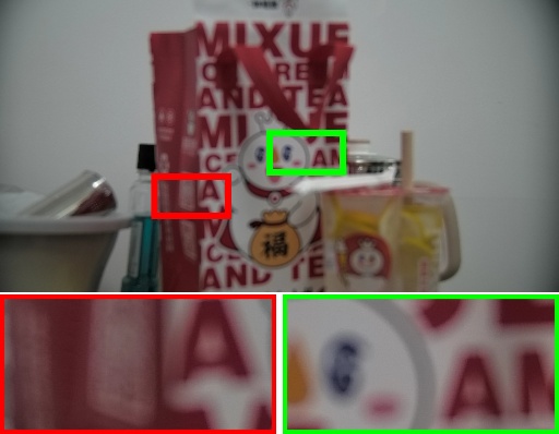
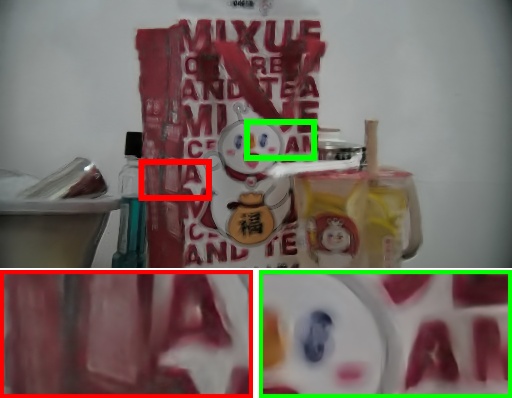
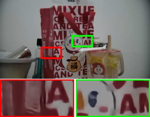
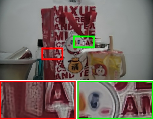
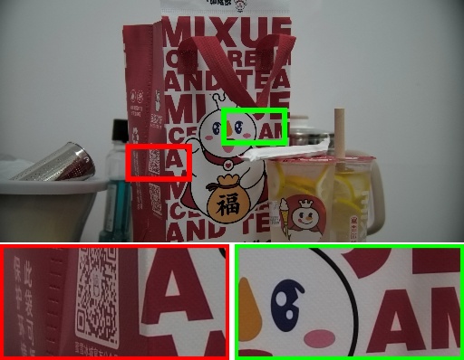
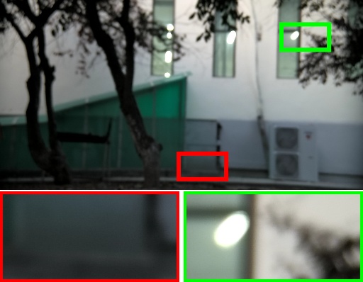
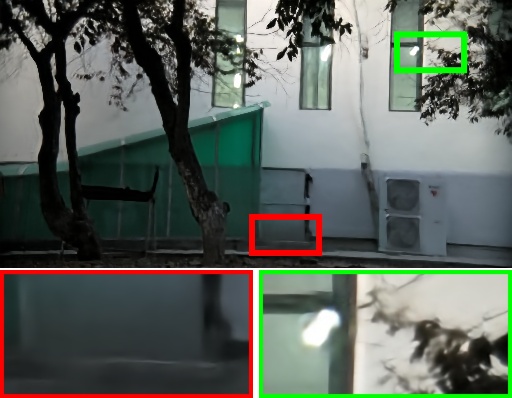
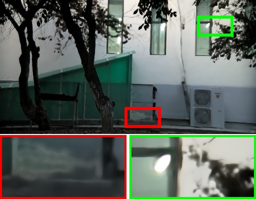
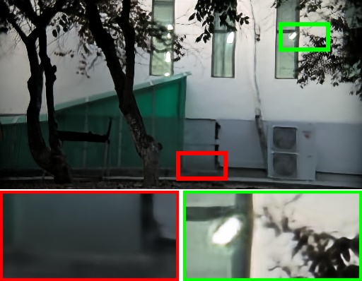
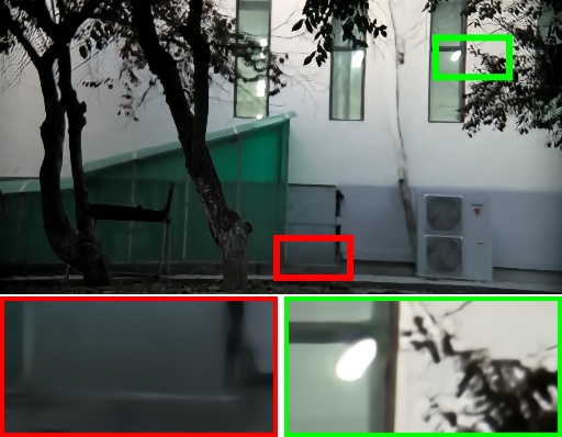
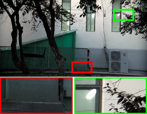
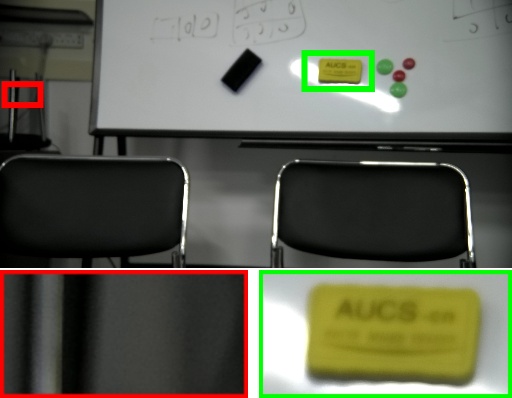
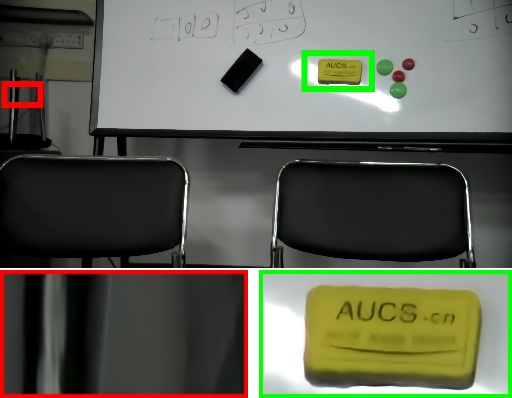
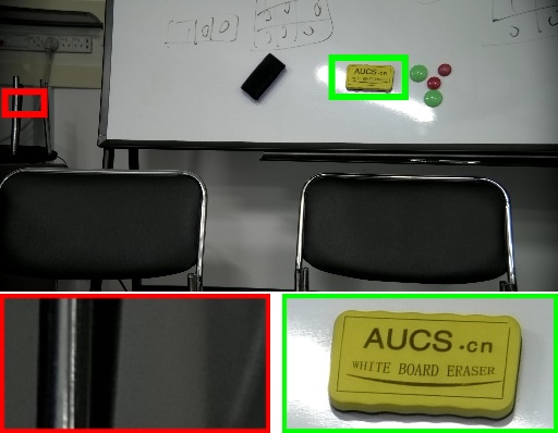
Input DMPHN MPRNet DPDNetS MPRNet* GT

Figure 7: Visual comparison between different methods on SDD dataset. With the proposed JDRL framework applied, MPRNet* performs visually better than the original MPRNet in terms of textures and structures.

New Dataset for Single Image Defocus Deblurring

Considering that DPDD is originally developed for dual-pixel defocus deblurring, we establish a new dataset named SDD for single image defocuse deblurring. In particular, a HUAWEI X2381-VG camera is employed. The DoF of this camera can be adjusted by vertically moving the lens or by changing its aperture size. We totally capture 150 blurry/sharp image pairs, each of which is of resolution $4096\times 2160$. These image pairs are split into a training set with 115 image pairs and a testing set with 35 image pairs. Similar to (Abuolaim and Brown 2020), the training image pairs are resized and cropped into 4,830 patches of size $512\times 512$. The SDD dataset covers a variety of indoor and outdoor scenes. There are 50 indoor scenes and 65 outdoor scenes in the training set, and 11 indoor scenes and 24 outdoor scenes in the testing set. Sample images from SDD dataset are exhibited in Fig. 6.

When collecting our SDD dataset, we also try to keep alignment between training pairs, but misalignments are inevitable for the consumer camera and collecting settings. For example, due to the fact that adjusting the aperture size will cause illumination change between blur and sharp images, we adjust DoF mainly by moving the lens back and forth. Only when the moving range is not enough for the desired DoF, we then change the aperture size, hence limiting the illumination change to small amounts. As a result, misalignment is inevitable during the capturing process. In practice, two types of misalignment would come up in tandem with the establishment of SDD dataset: zoom misalignment and shift misalignment, which are caused by the vertical and horizontal movement of camera lens, respectively (see Fig. 5). Misalignments in SDD dataset are usually more severe than DPDD dataset, and SDD is a testing bed for validating the effectiveness of our JDRL.

Experiments

Implementation Details

The source code, SDD dataset and the supplementary file are available at https://github.com/liyucs/JDRL. The source code is implemented in Pytorch (Paszke et al. 2019), and also we provide an implementation in HUAWEI Mindspore, which is available at https://github.com/Hunter-Will/JDRL-mindspore.

Configuration: During training, $\lambda$ is set as 0.35 for generating the calibration masks, and the maximal radius of blur kernels $m$ is set as 8. The baseline deblurring network $\mathcal{F}$ of JDRL is implemented as a vanilla U-Net structure, the details of which are described in suppl.

Datasets: The proposed JDRL framework is evaluated on three datasets: SDD, DPDD and RealDOF, where RealDOF is only used for testing the models trained on the DPDD dataset. The taining patches are all of size $512\times 512$. In the DPDD dataset, there are 350/76/74 image triplets for training/testing/validation, respectively. Each blurry image comes along with a sharp image. We use 350 blurry-sharp image pairs for training and 76 blurry images for testing.

Network training: During the initial stage of training, $\hat{\bm{I}}$ is of low quality, hence the predicted optical flow $\bm{\Phi}_{\bm{I}_{S}\rightarrow\hat{\bm{I}}}$ and $\bm{\Phi}_{\hat{\bm{I}}\rightarrow\bm{I}_{S}}$ are hardly informative. In this regard, $\bm{\Phi}_{\bm{I}_{S}\rightarrow\hat{\bm{I}}}$ is calculated by $\mathcal{F}_{flow}(\bm{I}_{S},\bm{I}_{B})$ at the beginning of training. After an initialization stage of $N$ training epochs, the optical flow is instead obtained by Eq. (2). Empirically, $N$ is set as 15 in our experiments to ensure the quality of $\hat{\bm{I}}$. The parameters of JDRL are initialized using the strategy proposed by He et al. (He et al. 2015), and are optimized using the Adam optimizer (DP and Ba 2015). The learning rate is initialized as 2$\times$10^-5 and is halved every 60 epochs. The entire training stage ends with 100 epochs.

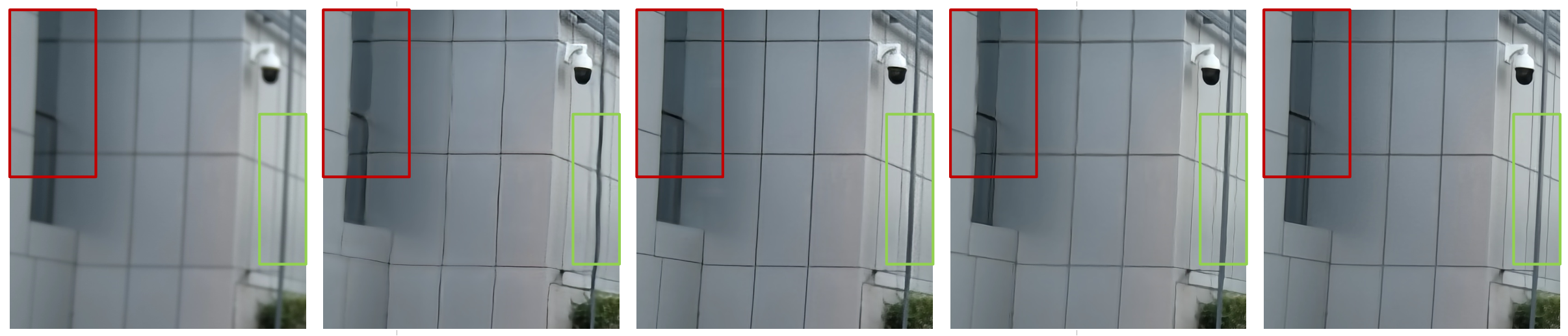
Input

UNet

UNet*

MPRNet

MPRNet*

Figure 8: Deformation artifacts by UNet and MPRNet, which can be alleviated by training with JDRL (UNet* and MPRNet*).

Experiments on SDD dataset

The proposed method is compared with SOTA single image defocus deblurring methods including JNB (Shi, Xu, and Jia 2015), EBDB (Karaali and Jung 2017), DMENet (Lee et al. 2019) and DPDNet_S (Abuolaim and Brown 2020). Since the former three methods are originally designed for defocus map estimation, we adopt non-blind deconvolution (Krishnan and Fergus 2009) to get the final estimated sharp images. Additionally, we retrain two SOTA motion deblurring methods DMPHN (Zamir et al. 2021) and MPRNet (Zhang et al. 2019) on the SDD dataset for extra comparison. Son et al. (Son et al. 2021) and IFAN (Lee et al. 2021) are excluded from comparison because Son et al. has not release the training code and IFAN requires additional dual-pixel data during training. As introduced before, the proposed JDRL framework can be applied to different existing methods. Therefore, we also replace the baseline deblurring network UNet with MPRNet, which achieves the best performance among all methods without using JDRL, for further comparison.

Table 1: Quantitive comparison between different methods on SDD dataset. ‘UNet’ and ‘UNet*’ refer to the baseline deblurring network without using and using the JDRL framework, respectively. ‘MPRNet*’ refers to MPRNet trained by JDRL framework.

Method	PSNR$\uparrow$	SSIM$\uparrow$	MAE$\downarrow$	LPIPS$\downarrow$
JNB	24.06	0.720	0.0400	0.443
EBDB	24.06	0.720	0.0398	0.442
DMENet	24.02	0.732	0.0395	0.426
DMPHN	25.00	0.769	0.0351	0.326
DPDNetS	24.81	0.760	0.0364	0.343
MPRNet	26.28	0.796	0.0293	0.302
UNet	24.62	0.758	0.0360	0.344
UNet*(Ours)	25.82	0.783	0.0320	0.305
MPRNet*(Ours)	26.88	0.810	0.0283	0.265

For evaluation, we use the testing set of SDD, which contains 35 blurry-sharp image pairs. Since the blurry images and ground-truth sharp images of SDD are misaligned, the evaluation metrics such as PSNR can not be directly calculated. In this regard, we use a pretrained PWCNet to compute the optical flow between $\hat{\bm{I}}$ and $\bm{I}_{S}$, and then deform $\bm{I}_{S}$ towards $\hat{\bm{I}}$. The evaluation metrics are then calculated between $\hat{\bm{I}}$ and the deformed ground-truth $\bm{I}_{S}^{w}$. Four metrics are adopted to quantitatively evaluate the compared methods: Peak Signal-to-Noise Ratio (PSNR), Structural Similiarity (SSIM) (Wang et al. 2004), Mean Absolute Error (MAE), and Learned Perceptual Image Patch Similarity (LPIPS) (Zhang et al. 2018).

Table 1 reports the evaluation results on SDD test set. By utilizing JDRL framework, both UNet* and MPRNet* outperform UNet and MPRNet respectively by a large margin. Moreover, it can be seen from Fig. 7 that MPRNet* performs favorably against the others in terms of both the restoration of image texture and the preservation of objects’ shapes. This is because existing methods are only trained with vanilla pixel-wise loss, by which spatial deformation is also learned during training. Taking the last row of Fig. 7 as example, the silver cylinder within the red bounding box is heavily distorted in all methods except for MPRNet*. Another example is given in Fig. 8, which shows that the issue of line distortion can be obviously alleviated by using JDRL.

Table 2: Quantitative comparison on DPDD. IFAN* and MPRNet* refer to IFAN and MPRNet trained by JDRL, respectively.

	GT	Deformed GT
Method	PSNR/SSIM/MAE/LPIPS	PSNR/SSIM/MAE/LPIPS
JNB	22.13/0.676/0.0560/0.480	21.30/0.692/0.0620/0.458
EBDB	23.19/0.713/0.0510/0.419	22.66/0.737/0.0540/0.397
DMENet	23.33/0.715/0.0506/0.411	22.89/0.740/0.0536/0.388
DPDNetS	24.39/0.750/0.0435/0.277	24.48/0.778/0.0435/0.262
Son et al.	25.22/0.774/0.0403/0.227	25.49/0.807/0.0398/0.212
IFAN	25.37/0.789/0.0394/0.217	25.86/0.825/0.0374/0.192
UNet	24.60/0.757/0.0426/0.281	24.63/0.785/0.0424/0.261
MPRNet	25.72/0.791/0.0385/0.235	26.03/0.820/0.0372/0.214
IFAN*	25.54/0.788/0.0389/0.207	26.09/0.826/0.0372/0.177
UNet*	24.73/0.762/0.0422/0.273	24.97/0.794/0.0413/0.248
MPRNet*	25.73/0.792/0.0384/0.232	26.21/0.825/0.0365/0.207

Table 3: Quantitative comparison on RealDOF. All the methods are trained on DPDD dataset, since RealDOF has no training set.

	GT	Deformed GT
Method	PSNR/SSIM/MAE/LPIPS	PSNR/SSIM/MAE/LPIPS
JNB	22.33/0.635/0.0514/0.598	21.02/0.651/0.0607/0.590
EBDB	22.38/0.640/0.0508/0.590	21.37/0.659/0.0581/0.579
DMENet	22.40/0.639/0.0508/0.593	21.38/0.658/0.0579/0.581
DPDNetS	22.85/0.668/0.0497/0.421	22.66/0.702/0.0504/0.397
Son et al.	23.98/0.716/0.0433/0.339	24.35/0.756/0.0414/0.308
IFAN	24.71/0.749/0.0407/0.306	25.39/0.794/0.0380/0.264
UNet	23.43/0.694/0.0463/0.396	23.51/0.729/0.0456/0.368
MPRNet	24.37/0.734/0.0413/0.346	24.66/0.771/0.0399/0.313
IFAN*	24.87/0.748/0.0395/0.288	25.61/0.793/0.0367/0.243
UNet*	23.55/0.696/0.0456/0.382	23.86/0.736/0.0441/0.349
MPRNet*	24.54/0.736/0.0403/0.339	24.90/0.775/0.0387/0.305

Experiments on DPDD and RealDoF datasets

For the DPDD dataset, apart from four methods mentioned above, the SOTA single image defocus deblurring methods Son et al. (Son et al. 2021) and IFAN (Lee et al. 2021) are also compared. It is worth noting that although the DPDD dataset is meant to be aligned, there actually exists slight misalignment as shown in Fig. 1. Therefore, we calculate the evaluation metrics in view of both ($\hat{\bm{I}}$ v.s. $\bm{I}_{S}$) and ($\hat{\bm{I}}$ v.s. $\bm{I}_{S}^{w}$). We also apply our JDRL framework to IFAN and MPRNet (denoted by IFAN* and MPRNet*). All the evaluated methods are tested on both DPDD test set and RealDOF dataset. The experimental results are reported in Table 2 and Table 3.

From Table 2 and Table 3, we have a similar observation as in Table 1, i.e., the learning-based methods outperform the traditional ones, and the performance of UNet, IFAN and MPRNet can be notably improved on DPDD and RealDOF test sets, when they are embedded into our proposed JDRL. By tolerating the slight misalignment existing in DPDD dataset, JDRL contributes to better performance on both testing sets of DPDD and RealDoF. Additionally, since the evaluated methods are only trained on DPDD dataset, the improved performance on RealDOF also indicates the generalizing ability of JDRL. The visual comparison on DPDD is given in suppl.

Ablation Study

Six network variants are designed to analyze the performance of JDRL on SDD dataset in terms of its different components: #1: the baseline network; #2: without the bi-directional optical flow deforming process; #3: without the calibration mask; #4: without the reblurring module $\mathcal{M}_{r}$; #5: without the isotropic design; #6: without the branch of $\mathcal{R}_{wpn}$. Variants #4, #5 and #6 are designed to prove the effectiveness of $\mathcal{M}_{r}$. The baseline deblurring network (UNet) is employed for all six ablative experiments.

The quantitative results are reported in Table 4. From #1 and #2, we can see that the absence of the deforming process considerably downgrades the network performance. Besides, the network performance gets slightly improved by incorporating the calibration mask, which is indicated by #3. From #4, we can see that the absence of $\mathcal{M}_{r}$ heavily impairs the overall network performance. Finally, the reuslts of #5 and #6 prove that the isotropic design and $\mathcal{R}_{wpn}$ in $\mathcal{M}_{r}$ both benefit the reblurring process. The visual results and more details are included in supplementary materials.

Table 4: Ablation study on SDD dataset.

Category	PSNR/SSIM/MAE/LPIPS
#1 Baseline	24.62/0.758/0.0360/0.344
#2 w/o Cycle Deformation	24.80/0.758/0.0353/0.347
#3 w/o Calibration Mask	25.78/0.780/0.0326/0.309
#4 w/o $\mathcal{M}_{r}$	25.58/0.777/0.0335/0.311
#5 w/o Isotropic Design	25.68/0.778/0.0329/0.311
#6 w/o $\mathcal{R}_{wpn}$	25.74/0.778/0.0330/0.332
Final	25.82/0.783/0.0320/0.305

Conclusion

In this paper, we proposed a joint deblurring and reblurring learning (JDRL) framework for single image defocus deblurring. On the one hand, a deblurring module $\mathcal{M}_{d}$ with spatially adaptive deblurring loss is developed to tolerate misalignment between image pairs with the help of optical flow. Strategies of calibration mask and cycle deformation are employed to enhance the robustness of deformation process. On the other hand, a spatially invariant reblurring module ($\mathcal{M}_{r}$) is proposed, which consists of a kernel prediction network ($\mathcal{R}_{kpn}$) and a weight prediction network ($\mathcal{R}_{wpn}$). The spatial consistency between deblurred image and blurry image is guaranteed by the isotropic blur kernels predicted by $\mathcal{R}_{kpn}$. The proposed JDRL framework can be widely adopted, since it is not coupled with deblurring network architecture. Experimental results on SDD, DPDD and RealDOF datasets validate the effectiveness of JDRL. Our newly established SDD dataset for single image defocus deblurring would also benefit future research in this field.

Learning Single Image Defocus Deblurring with Misaligned Training Pairs
   
Supplemental Materials

\begin{overpic}[width=505.89pt]{figs/kernel} \end{overpic}

Figure 9: Isotropic blur kernels of different kernel sizes generated by $\mathcal{R}_{kpn}$. We randomly visualize one example for each kernel size.

Spatially Invariant Reblurring Module

Our reblurring network $\mathcal{R}$ is proposed for generating the reblurred image $\hat{\bm{I}}_{B}$, which is then supervised by input image $\bm{I}_{B}$. In this process, isotropic blur kernels predicted by $\mathcal{R}_{kpn}$ are used to guarantee the spatial consistency between the deblurred result $\hat{\bm{I}}$ and $\bm{I}_{B}$. Several examples of isotropic blur kernels generated by $\mathcal{R}_{kpn}$ are given in Fig. 9.

Discussion on the Misalignment Problem

The phenomenon of misalignment widely exists in real-world datasets, leading to undesirable influence on relevant visual tasks. Thus, researchers have proposed approaches in various aspects to tackle the misalignment problem.

In the field of image translation, a common strategy to deal with misalignment is cycle-consistency (Zhu et al. 2017). However, the method based on cycle-consistency may produce multiple solutions and is sensitive to perturbation. Therefore, methods like RegGAN (Kong et al. 2021) have been proposed to address this problem. The spatial deformation predicted by RegGAN is a single-direction process. By contrast, our cycle deformation mechanism works in a bi-directional manner. Moreover, we adopt an dedicated isotropic kernel generation module to maintain spatial consistency during the reblurring process.

Zhang et al. (Zhang et al. 2019b) propose a contextual bilateral loss to address the misalignment problem in super resolution tasks. We have also tried adapting contextual loss to deblurring problems. However, it turned out that the UNet trained with contextual bilateral loss achieved inferior performance compared with the UNet trained with JDRL (24.58/0.756/0.0355/0.326 vs. 25.82/0.783/0.0320/0.305 in terms of PSNR/SSIM/MAE/LPIPS), which is partially attributed to its incapability in dealing with severe misalignment.

Ablation Study

The visual results of ablation study from the main text are presented in Fig. 10 and Fig. 11. In the ablation study, six variants of the original network are designed to investigate the significance of different network components: #1: baseline network, i.e., a vanilla UNet; #2: without the optical flow deforming process; #3: without the calibration mask; #4: without the reblurring module $\mathcal{M}_{r}$; #5: without the isotropic design; #6: without the weight prediction network $\mathcal{R}_{wpn}$, i.e., using only fixed-size kernels (15$\times$15) predicted by $\mathcal{R}_{kpn}$.

As shown in Fig. 10, the results from #1 and #2 have fewer textural details and could suffer from shape deformation. This is because the pixel-wise loss encourages positionally consistent mapping between the input and output, while such mapping is hard to learn between unaligned image pairs without the deforming process. #3 performs better than #1 and #2 yet still have less textures than the final model due to the missing calibration mask.

By comparing the visual results in Fig. 11, one can see that the network performance gets considerably downgraded without the reblurring module (#4). The absence of isotropic kernels (#5) would also lead to inferior visual results, since the output of reblurred module can be misaligned with the input image in this case. What’s more, the network performance gets impaired without the kernel prediction network $\mathcal{R}_{wpn}$ (#6). The function of $\mathcal{R}_{wpn}$ (#6) is generating kernels of different blurry levels, such that resulting in reblurred ouputs that are more coherent with the natural state of blurry images.

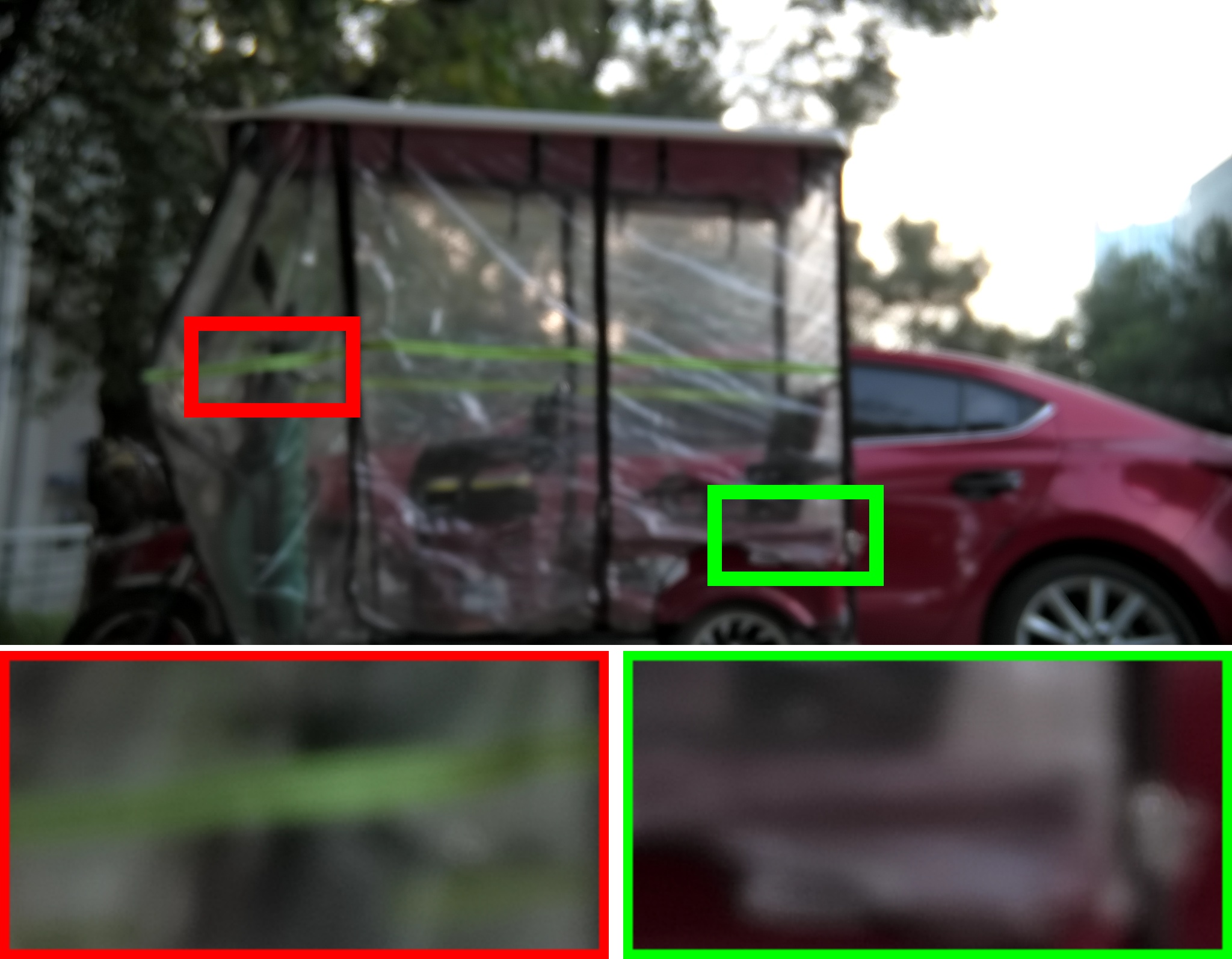
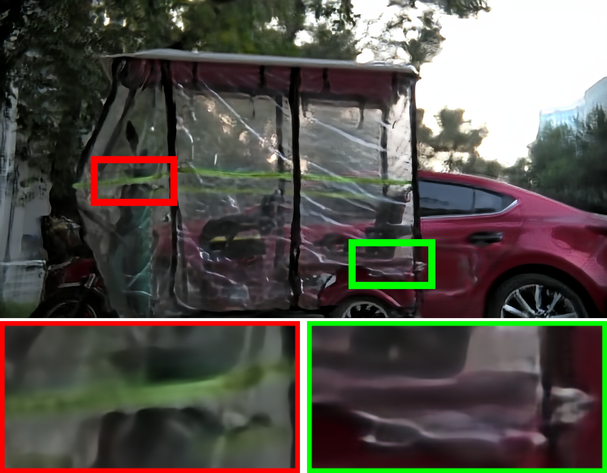
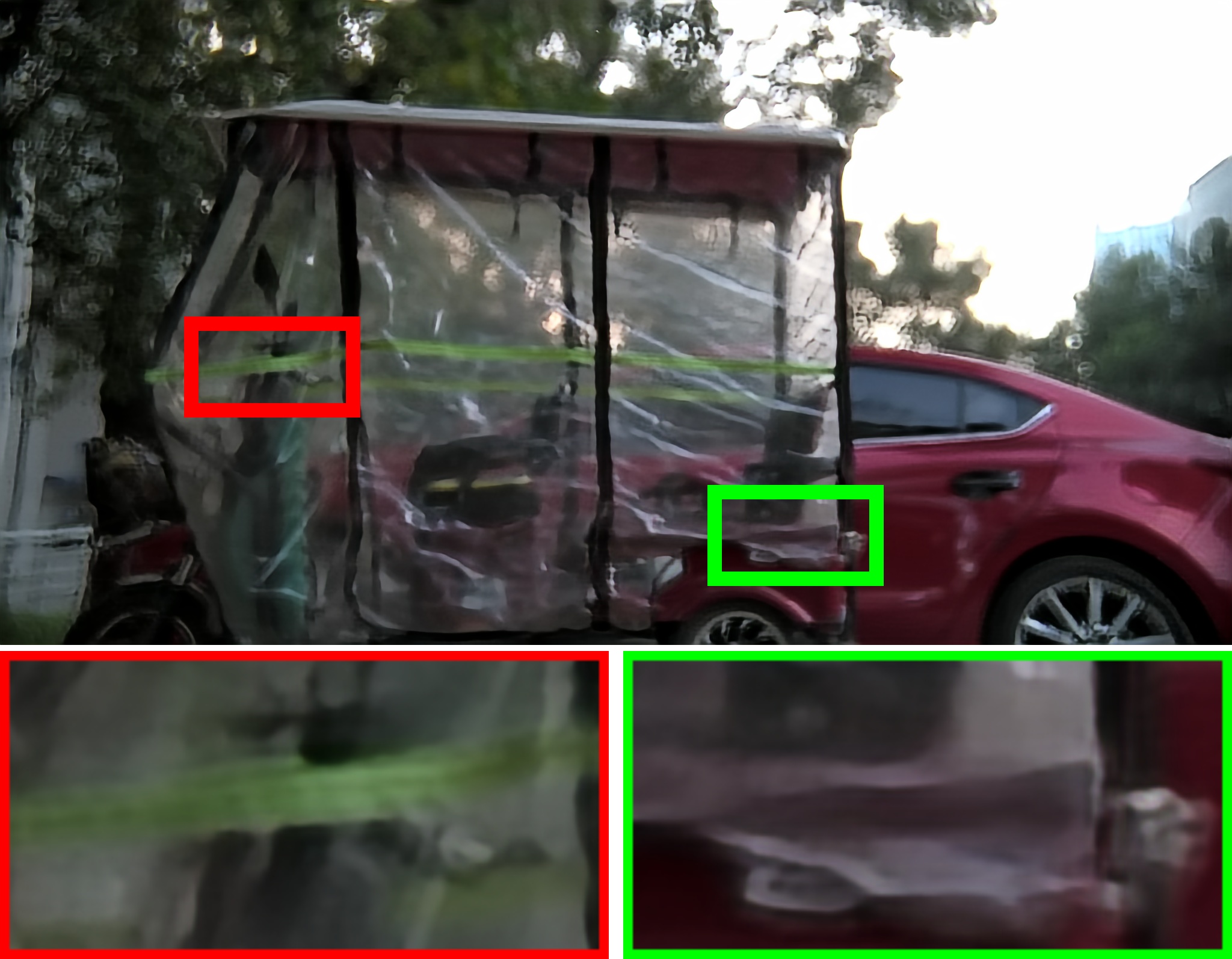
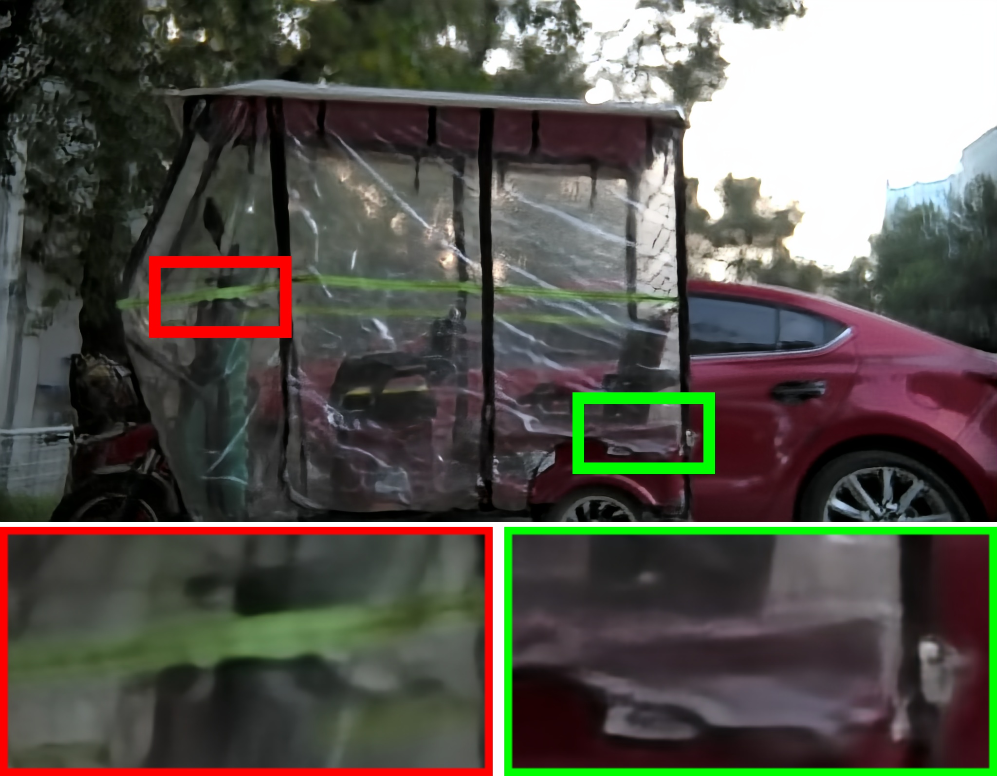
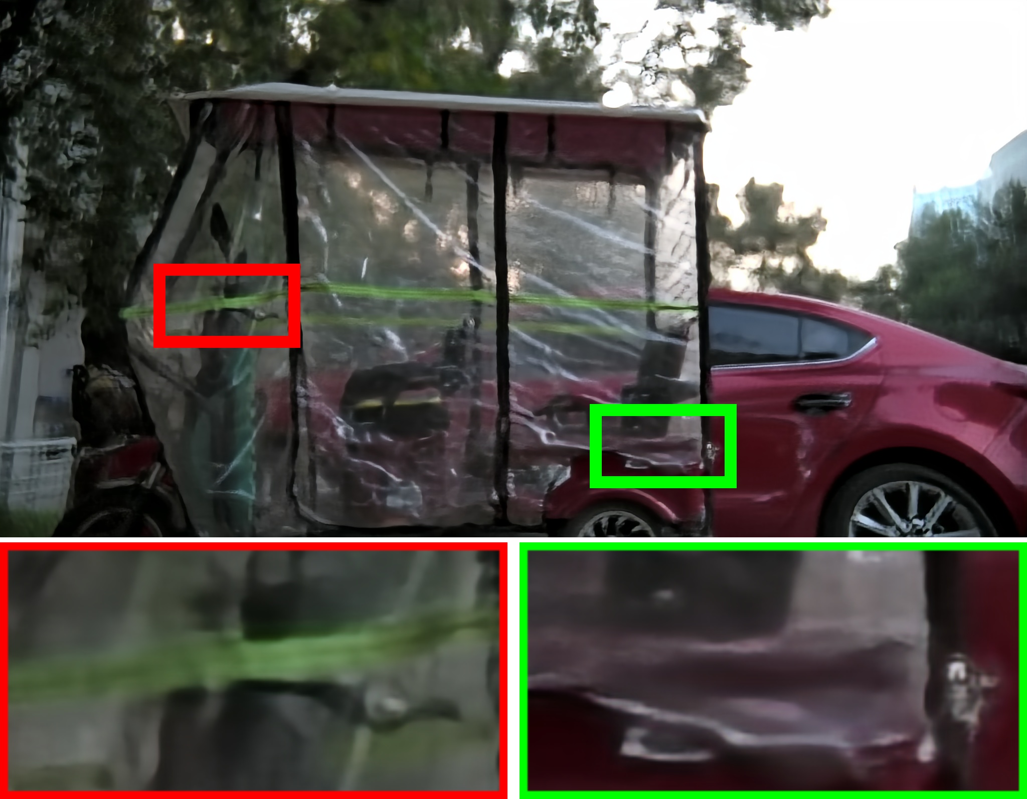
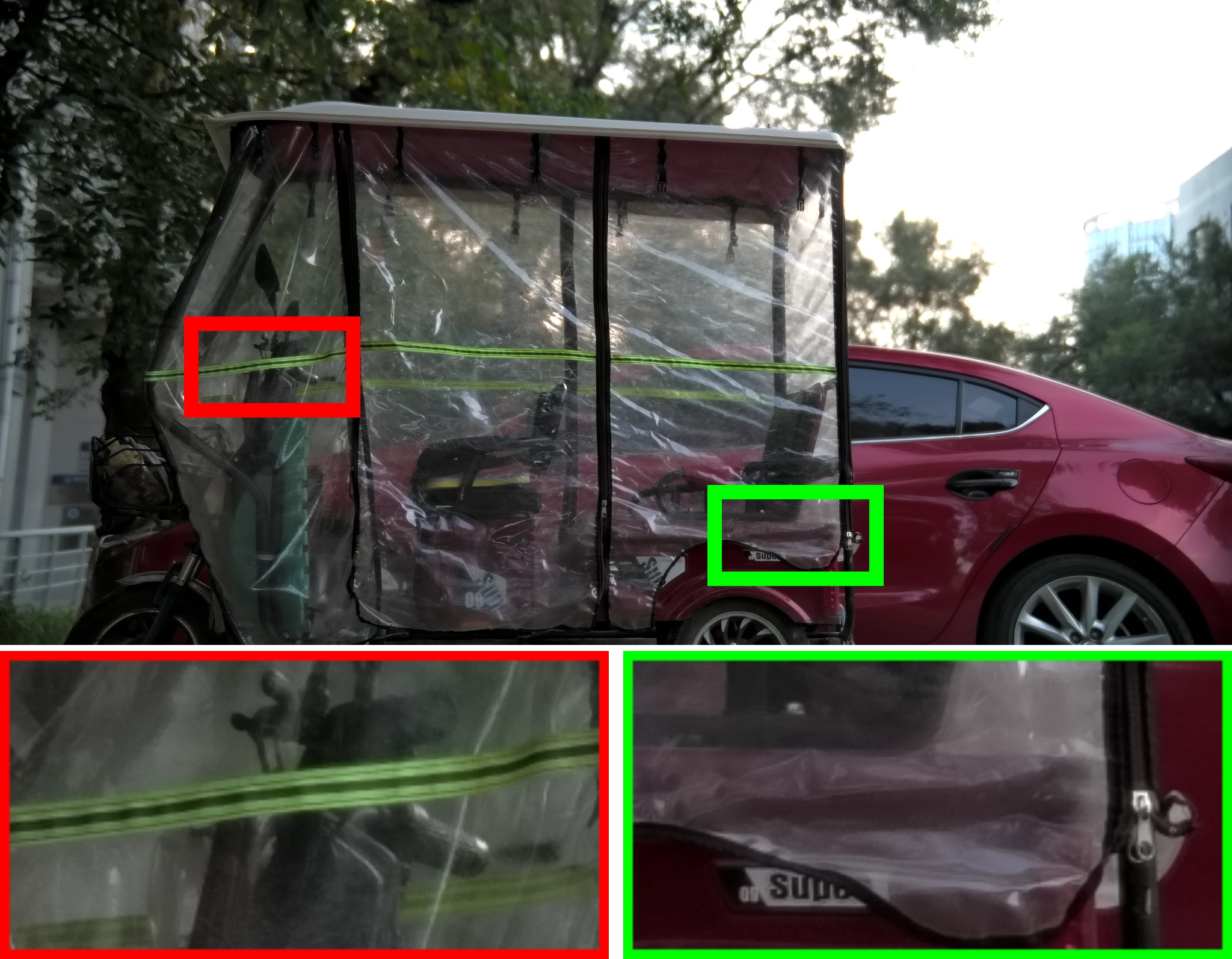
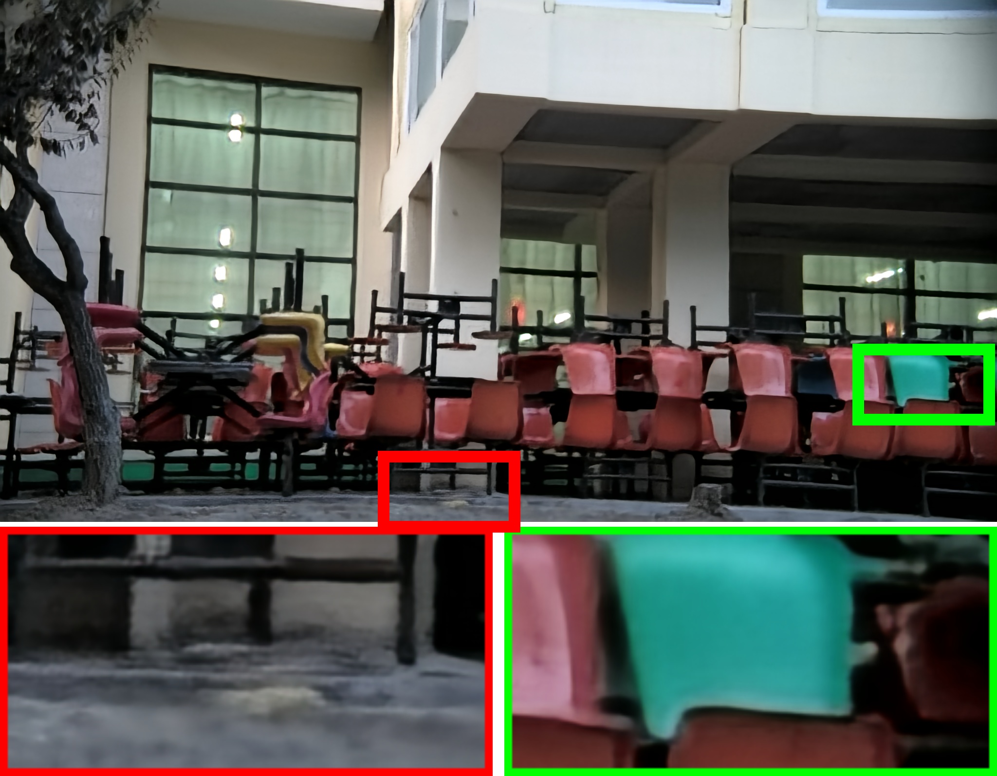
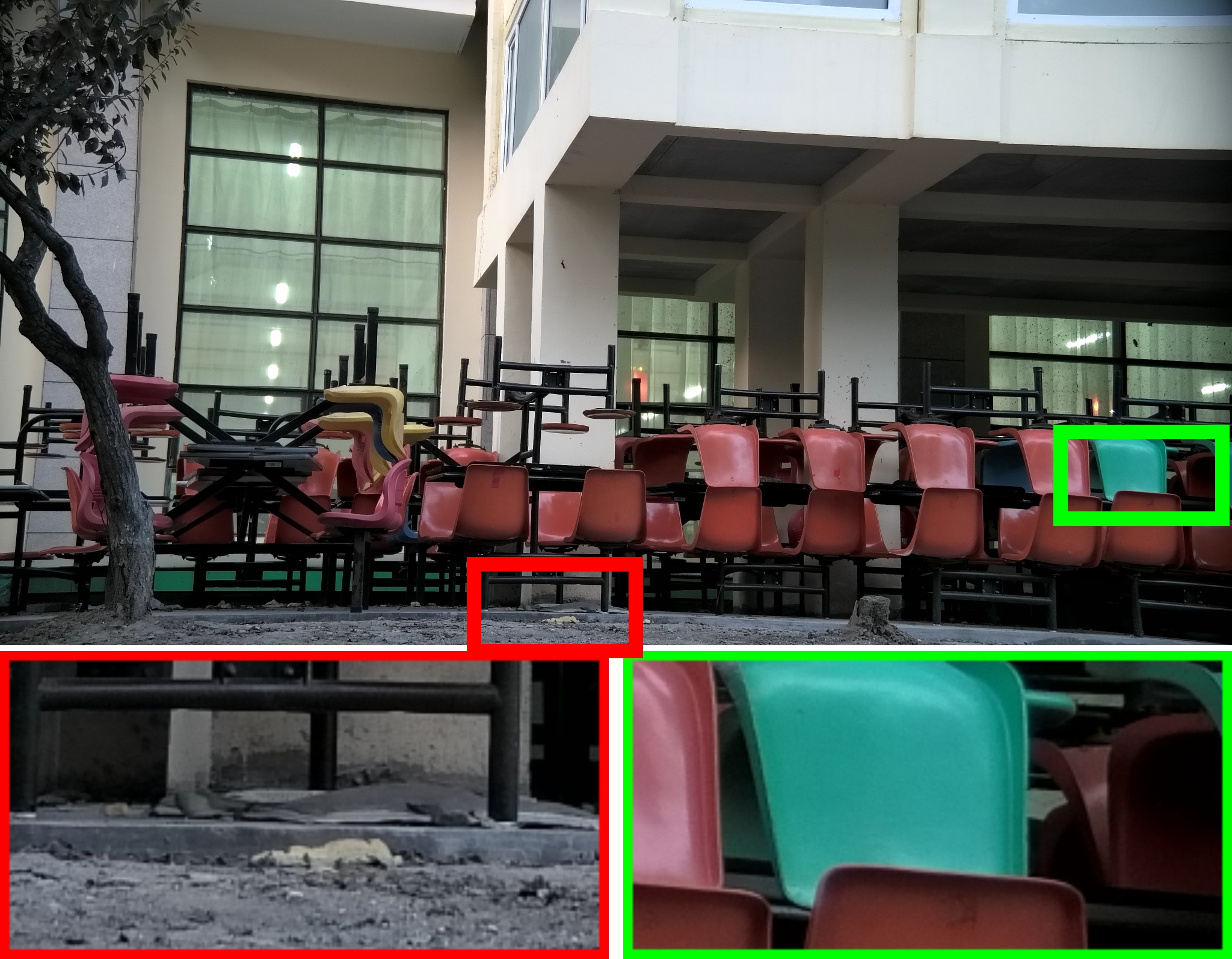
Input # 1 # 2 # 3 Final GT

Figure 10: Visual results of ablation study on SDD dataset.

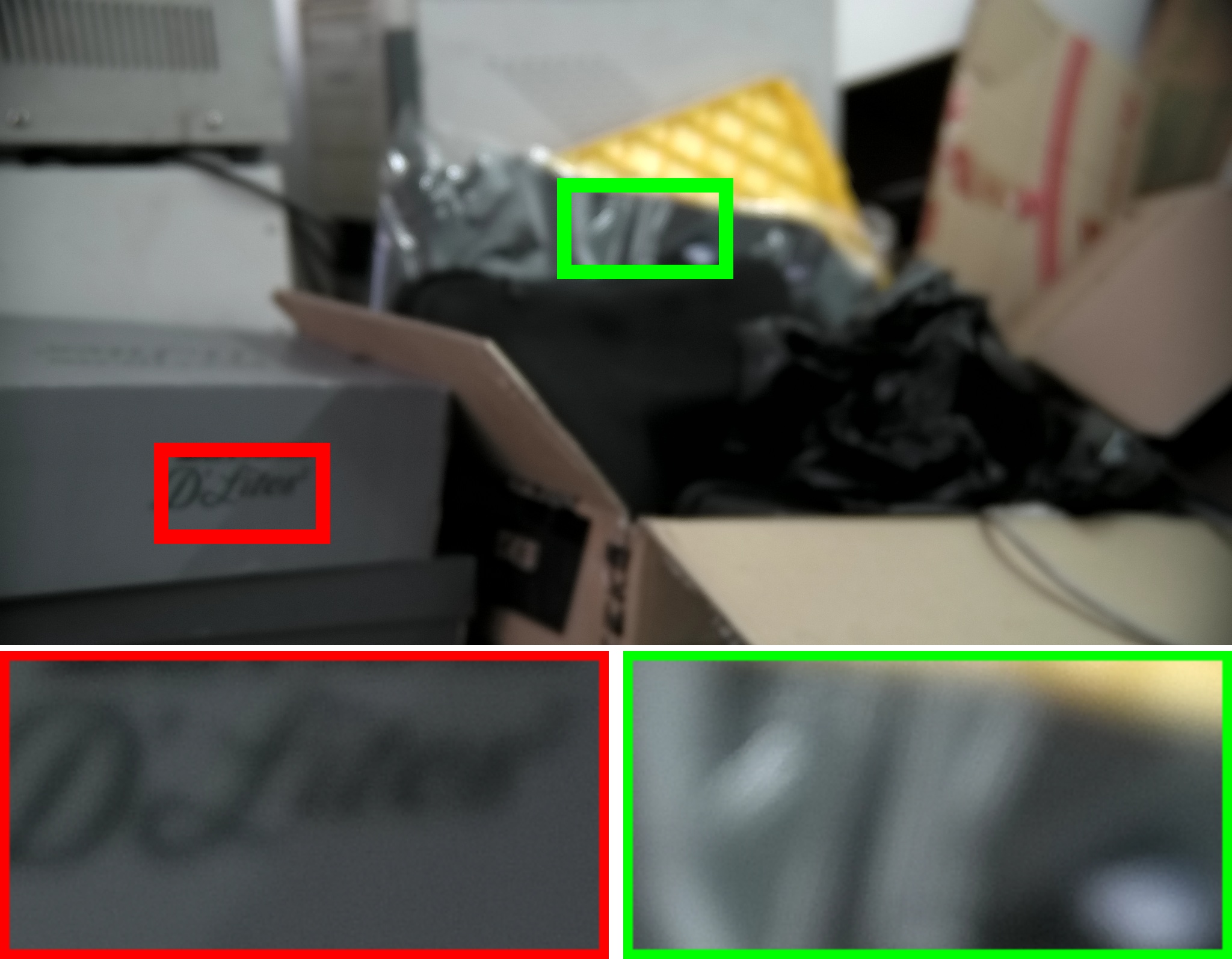
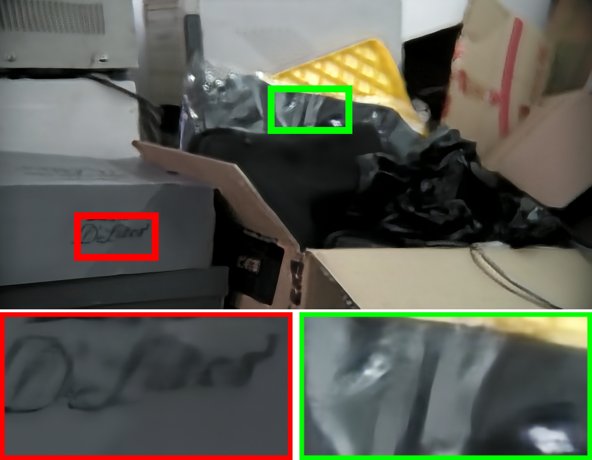
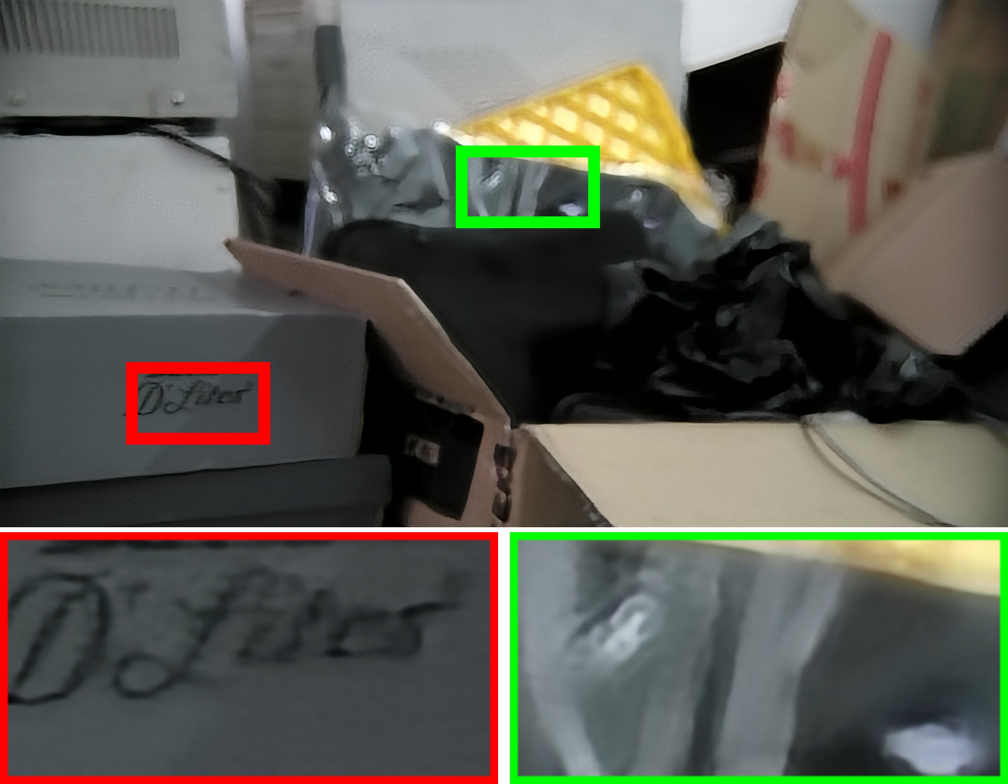
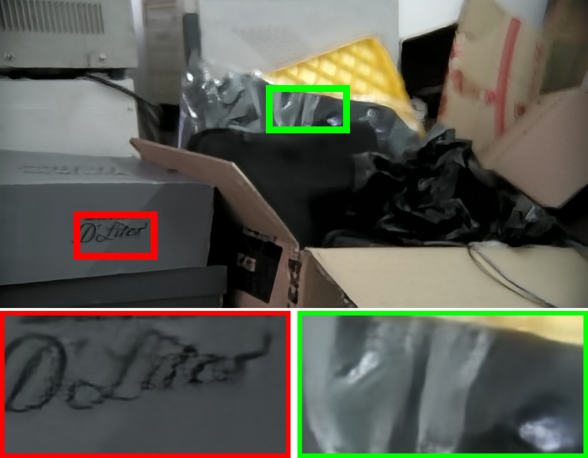
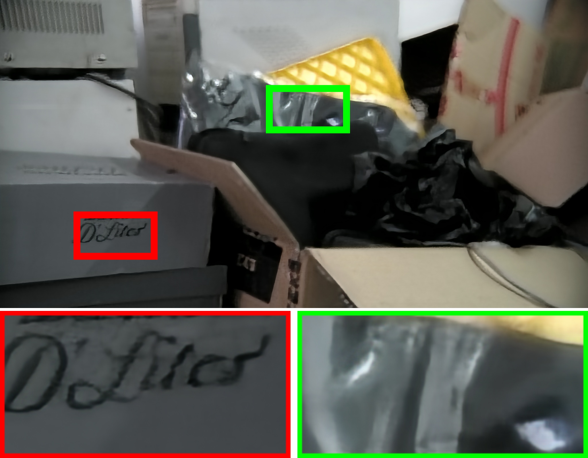
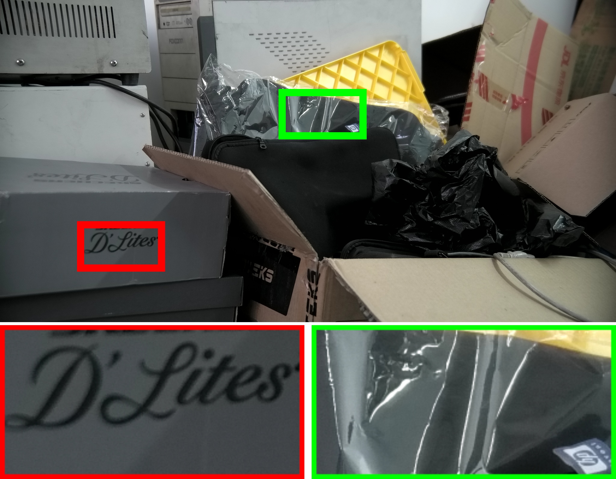
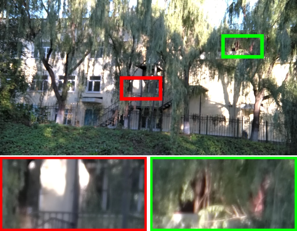
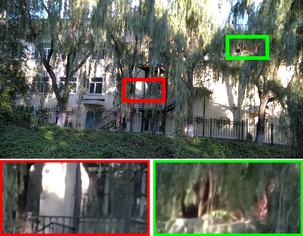
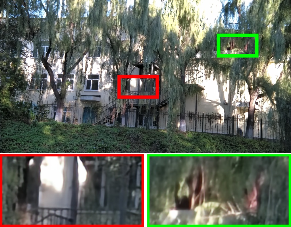
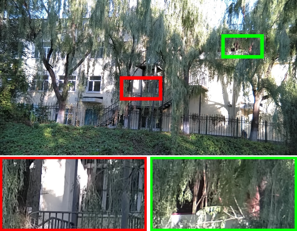
Input # 4 # 5 # 6 Final GT

Figure 11: Visual results of ablation study on SDD dataset.

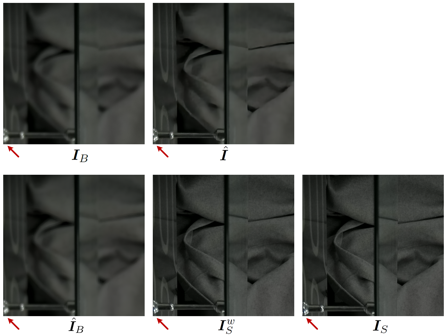
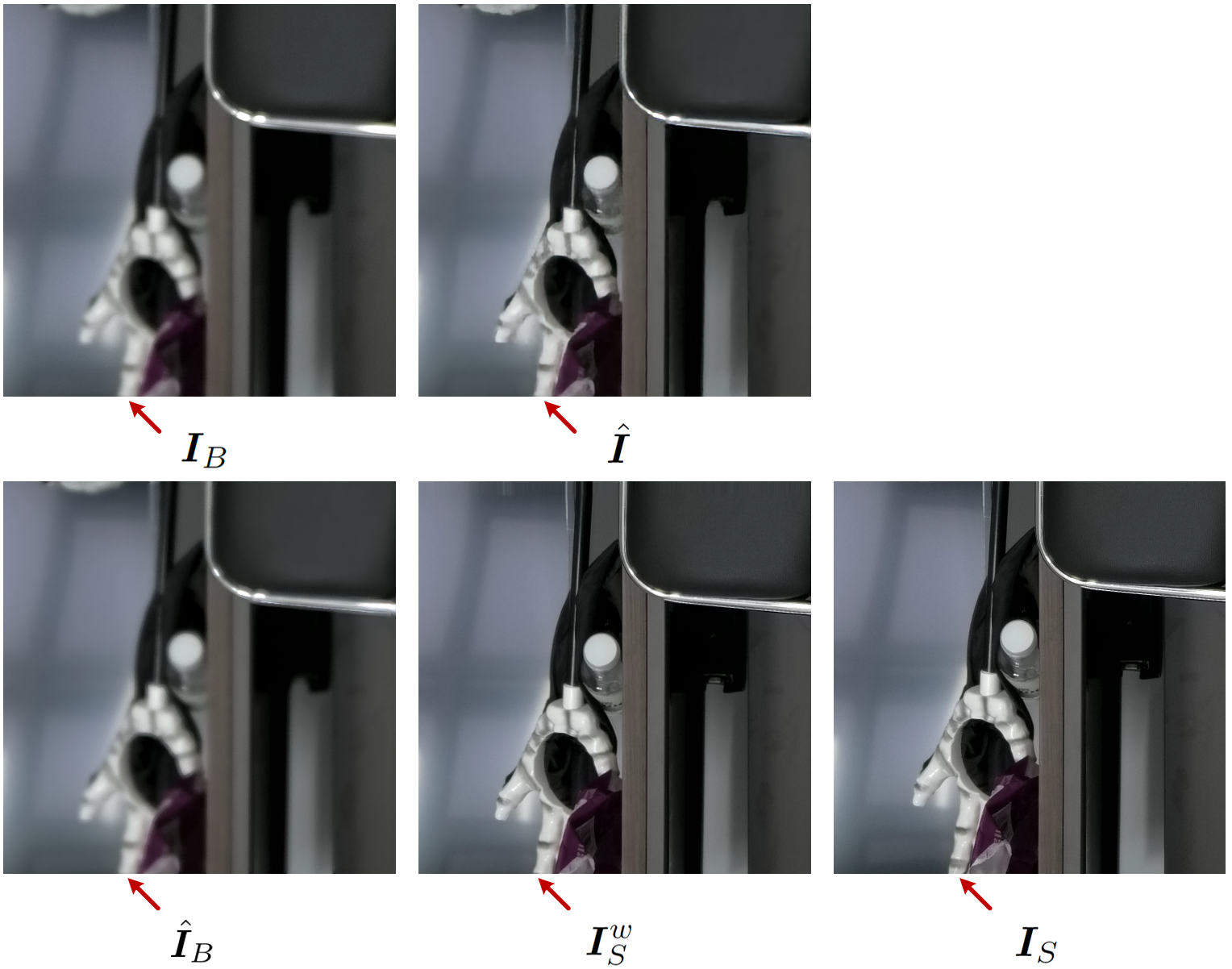
Figure 12: Visualization of reblurred results and deformed ground-truth sharp images.

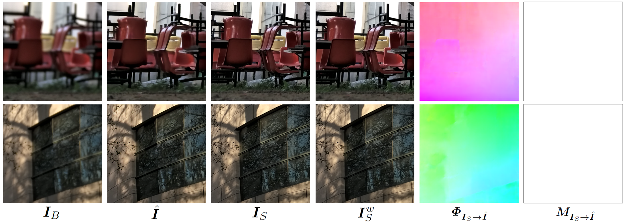
(a) When the optical flow is correctly estimated, the values of calibration mask are all 1 (i.e, all white in RGB color space).

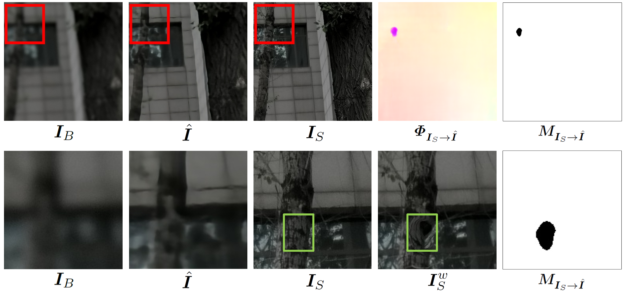
(b) When the optical flow is facing estimation error, the ground-truth sharp image will also be wrongly deformed (note the region marked by green rectangles). In this circumstance, the calibration mask will filter out this adverse region, in order to prevent it from influencing the subsequent loss calculation (Eq. (5)).

Figure 13: Illustration of how calibration masks work.

Calibration Mask

The functionality of calibration masks is illustrated in Fig 13. Because of the characteristic of optical flow, there should not be any sudden change in the magnitude of optical flow values across the image. Based on such motivation, we employ calibration masks to identify the abnormal change of optical flow values according to Eq. (4), such that the calculation of deblurring loss (Eq. (5)) will not be influenced by the inaccurately estimated optical flows.

We also give examples of reblurred result $\hat{\bm{I}}_{B}$ and deformed ground-truth sharp image ${\bm{I}}_{S}^{w}$ in Fig. 12. It can be seen that that $\bm{I}_{B}$, $\hat{\bm{I}}$, $\hat{\bm{I}}_{B}$ and ${\bm{I}}_{S}^{w}$ are spatially consistent, while $\bm{I}_{S}$ has a misalignment with all of them.

Network Details

Our baseline deblurring network is designed as a U-Net structure, whose detailed structures are shown in Table 1. The architecture details of $\mathcal{R}_{kpn}$ and $\mathcal{R}_{wpn}$ are presented in Table 2.

Comparison with DRBNet

DRBNet adopts an extra light field dataset LFDOF in the training stage, which considerably improves the network performance. A comparison with DRBNet is provided in this section. PSNR/SSIM/LPIPS metrics are shown in Table 5. By adopting the same DPDD training set, Ours* is better than DRBNet on both RealDOF and DPDD. On RealDOF, it is reasonable that DRBNet with more training sets DPDD+LFDOF is better than Ours* only with DPDD training set.

Table 5: PSNR/SSIM/LPIPS comparison between DRBNet and ours.

Method	Training set	RealDOF test set	DPDD test set
DRBNet	DPDD + LFDOF	25.75/0.771/0.257	25.73/0.791/0.183
DRBNet	DPDD	24.70/0.744/0.337	25.47/0.787/0.246
Ours	DPDD	24.87/0.748/0.288	25.73/0.792/0.232

More Results

In this section, more visual results on SDD, DPDD and RealDOF dataset are presented in Fig. $\sim$ Fig. 19. It can be seen that the methods trained by our JDRL framework (UNet*, MPRNet* and IFAN*) outperform their vanilla counterparts (UNet, MPRNet and IFAN) in view of sharp textures and undistorted shapes. By using JDRL, the lines and contours of objects from the input images are better preserved in the deblurring output. The JDRL versions of DPDNet_S and Son et al. are not provided because DPDNet_S is basically a vanilla UNet and Son et al. have not released their training codes.

Table 6: The structure of baseline deblurring network. The structure of encoder is shown in the left column and the structure of decoder is shown in the right column. For convolution layers, kernel size=3. For maxpooling layers, kernel size=2, stride=2. For dropout layers, we set the random dropping probability as 0.4. When doing upsampling, the scale factor is set as 2.

Encoder			Decoder
Layer	Output size	Filter	Layer	Output sizs	Filter
Conv,ReLU	$512\times 512$	$3\rightarrow 64$	Upsample,Conv	$32\times 32$	$1024\rightarrow 512$
Conv,ReLU	$512\times 512$	$64\rightarrow 64$	Concat	$32\times 32$	$(512+512)\rightarrow 1024$
MaxPool	$256\times 256$	-	Conv,ReLU	$32\times 32$	$1024\rightarrow 512$
			Conv,ReLU	$32\times 32$	$512\rightarrow 512$
Conv,ReLU	$256\times 256$	$64\rightarrow 128$	Upsample,Conv	$128\times 128$	$512\rightarrow 256$
Conv,ReLU	$256\times 256$	$128\rightarrow 128$	Concat	$128\times 128$	$(256+256)\rightarrow 512$
MaxPool	$128\times 128$	-	Conv,ReLU	$128\times 128$	$512\rightarrow 256$
			Conv,ReLU	$128\times 128$	$256\rightarrow 256$
Conv,ReLU	$128\times 128$	$128\rightarrow 256$	Upsample,Conv	$256\times 256$	$256\rightarrow 128$
Conv,ReLU	$128\times 128$	$256\rightarrow 256$	Concat	$256\times 256$	$(128+128)\rightarrow 256$
MaxPool	$64\times 64$	-	Conv,ReLU	$256\times 256$	$256\rightarrow 128$
			Conv,ReLU	$256\times 256$	$128\rightarrow 128$
Conv,ReLU	$64\times 64$	$256\rightarrow 512$	Upsample,Conv	$512\times 512$	$128\rightarrow 64$
Conv,ReLU	$64\times 64$	$256\rightarrow 512$	Concat	$512\times 512$	$(64+64)\rightarrow 128$
Dropout	$64\times 64$	-	Conv,ReLU	$512\times 512$	$128\rightarrow 64$
MaxPool	$32\times 32$	-	Conv,ReLU	$512\times 512$	$64\rightarrow 64$
Conv,ReLU	$32\times 32$	$512\rightarrow 1024$	Conv,Sigmoid	$512\times 512$	$64\rightarrow 3$
Conv,ReLU	$32\times 32$	$1024\rightarrow 1024$
Dropout	$32\times 32$	-

Table 7: The architecture of $\mathcal{R}_{kpn}$ and $\mathcal{R}_{wpn}$.

$\mathcal{R}_{kpn}$				$\mathcal{R}_{wpn}$
Layer		Output size	Filter	Layer		Output sizs	Filter
	Conv	$512\times 512$	$6\rightarrow 64$		Conv	$512\times 512$	$6\rightarrow 64$
Resblock	Conv, Relu	$512\times 512$	$64\rightarrow 64$	Resblock	Conv, Relu	$512\times 512$	$64\rightarrow 64$
	Conv	$512\times 512$	$64\rightarrow 64$		Conv	$512\times 512$	$64\rightarrow 64$
Resblock	Conv, Relu	$512\times 512$	$64\rightarrow 64$	Resblock	Conv, Relu	$512\times 512$	$64\rightarrow 64$
	Conv	$512\times 512$	$64\rightarrow 64$		Conv	$512\times 512$	$64\rightarrow 64$
Resblock	Conv, Relu	$512\times 512$	$64\rightarrow 64$	Resblock	Conv, Relu	$512\times 512$	$64\rightarrow 64$
	Conv	$512\times 512$	$64\rightarrow 64$		Conv	$512\times 512$	$64\rightarrow 64$
	Conv	$512\times 512$	$64\rightarrow 35$		Conv	$512\times 512$	$64\rightarrow 8$

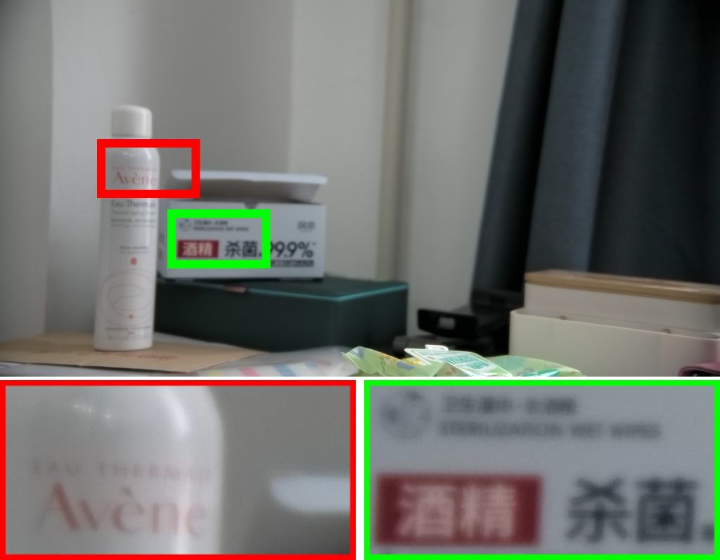
(a) Input

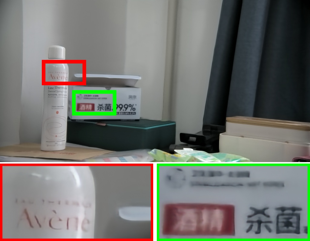
(b) UNet

(c) MPRNet

(d) DPDNet_S

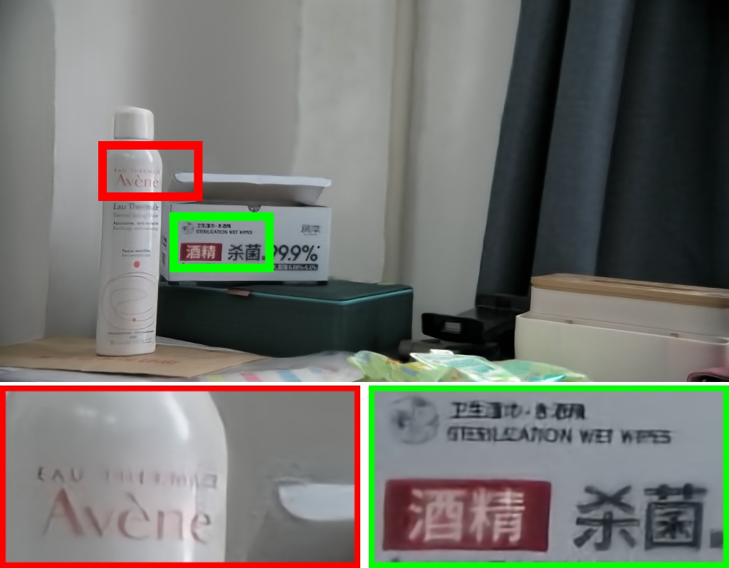
(e) DMPHN

(f) UNet*

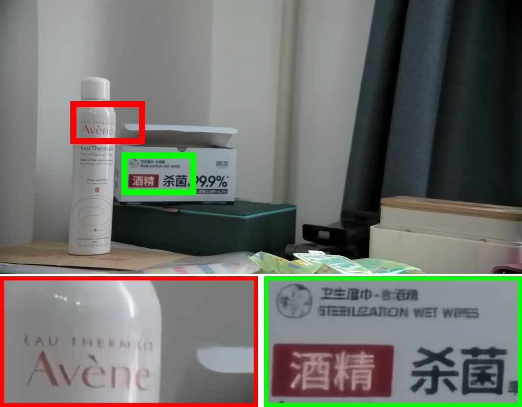
(g) MPRNet*

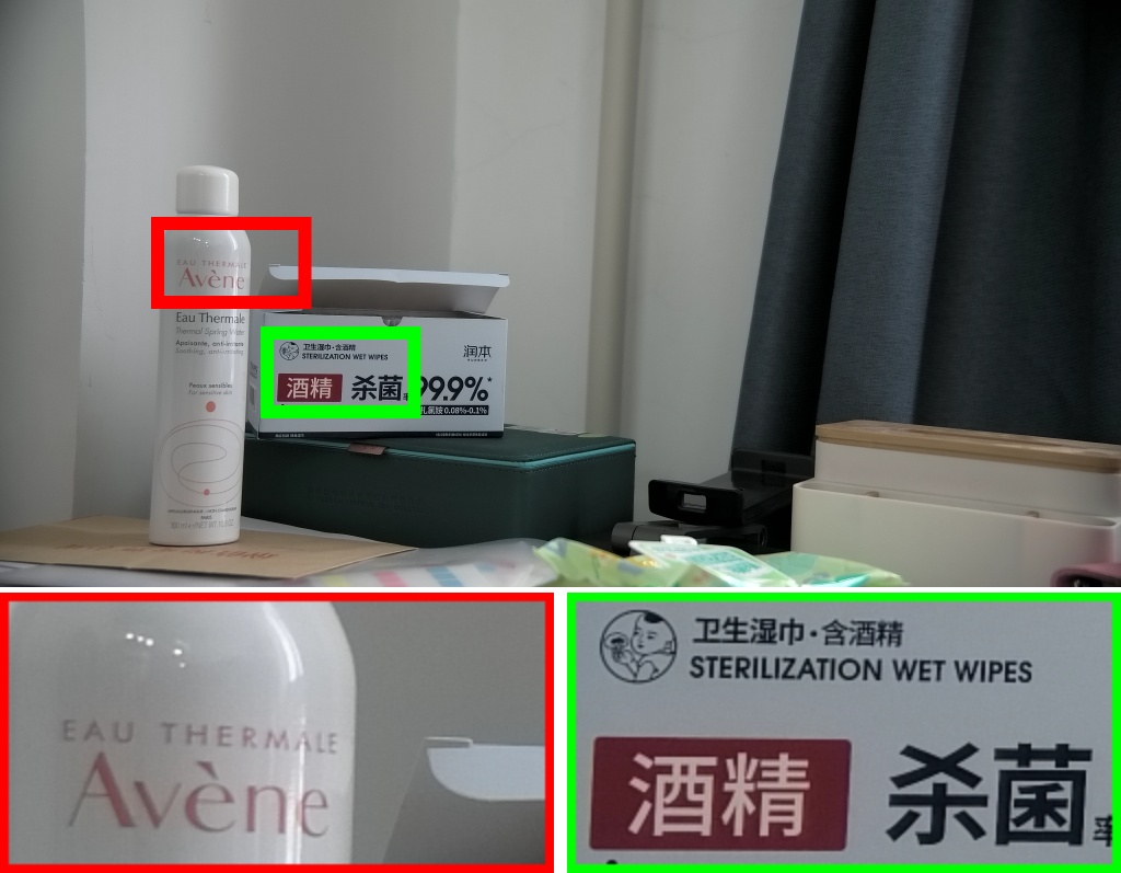
(h) GT

Figure 14: Visual comparison between different methods on SDD dataset.

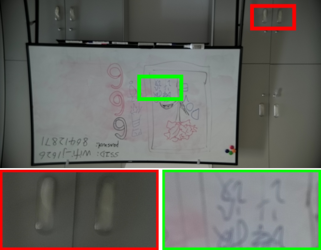
(a) Input

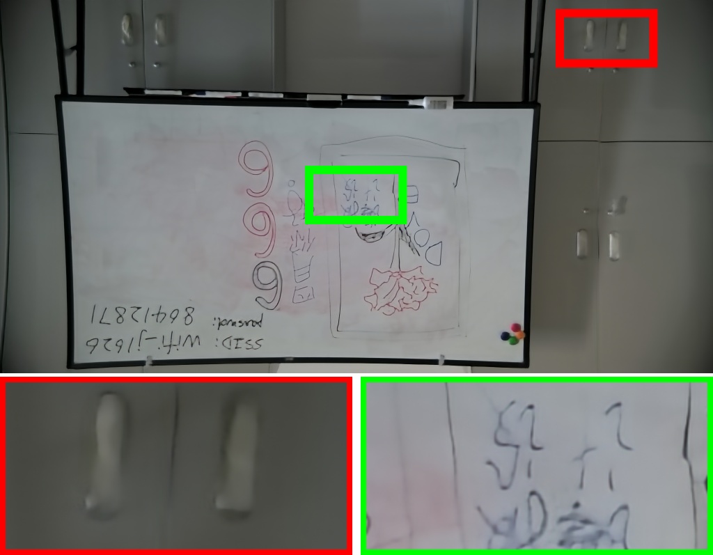
(b) UNet

(c) MPRNet

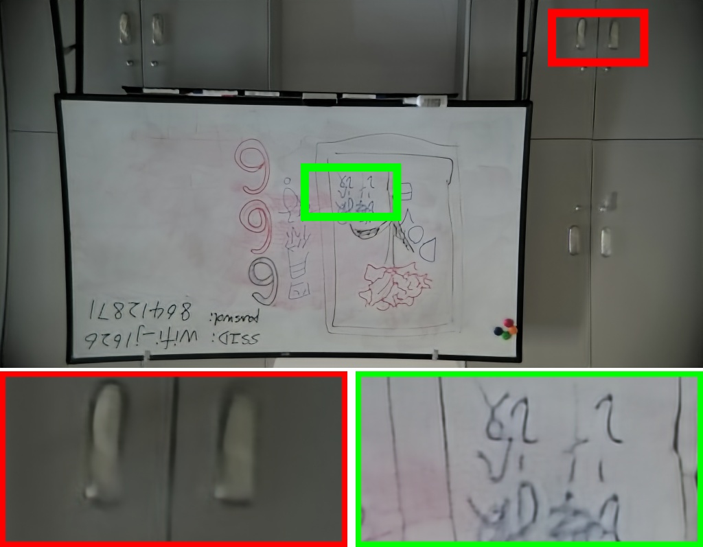
(d) DPDNet_S

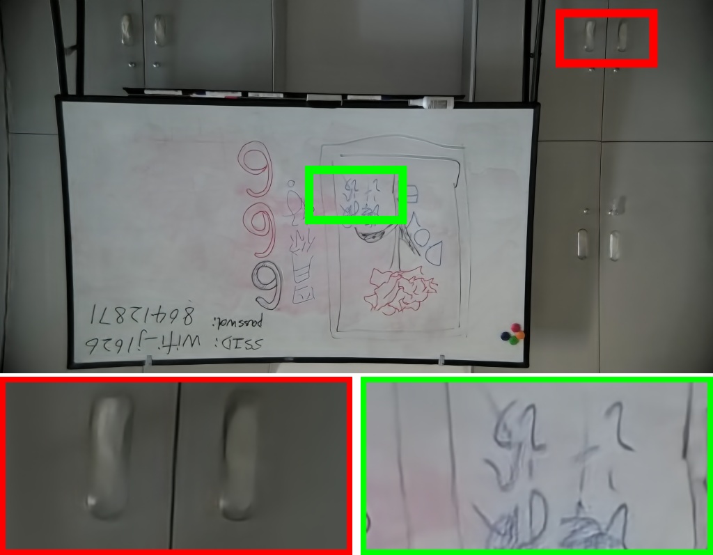
(e) DMPHN

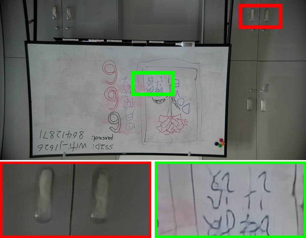
(f) UNet*

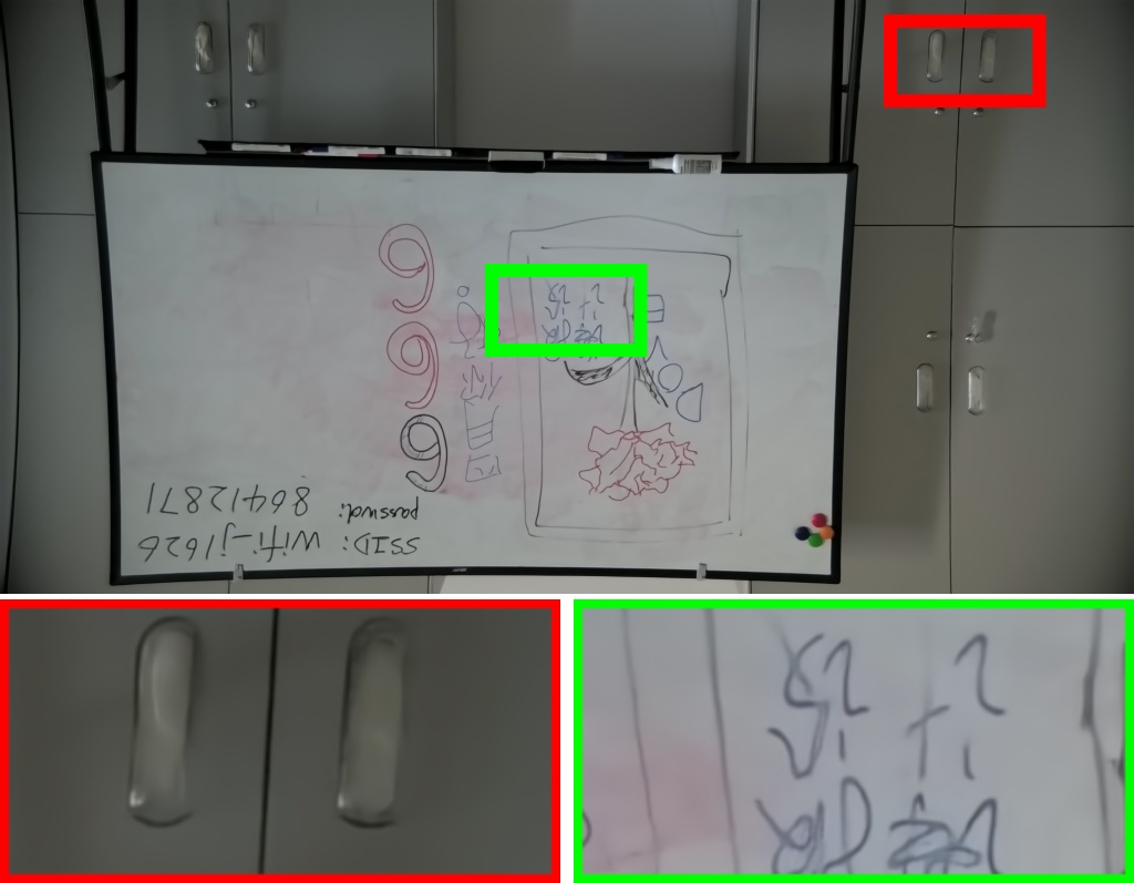
(g) MPRNet*

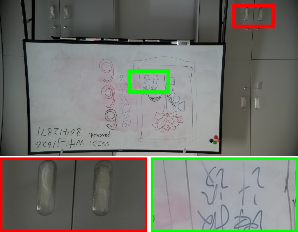
(h) GT

Figure 15: Visual comparison between different methods on SDD dataset.

(a) Input

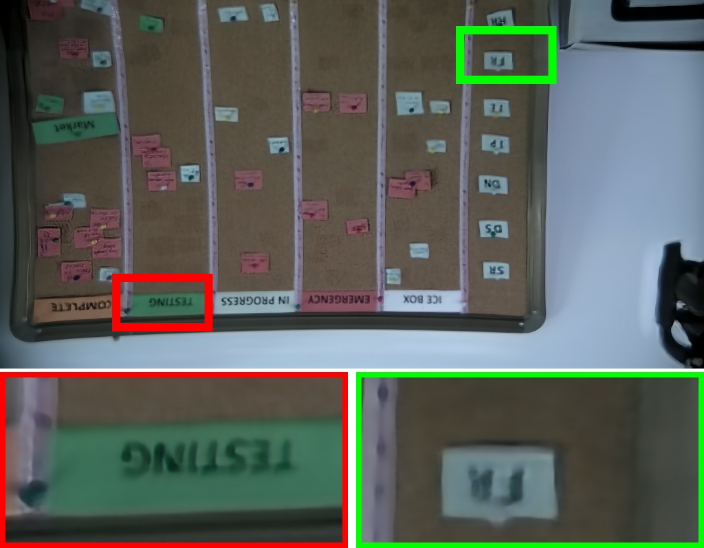
(b) UNet

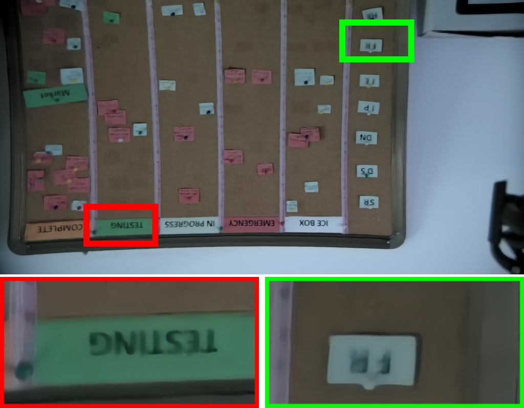
(c) MPRNet

(d) DPDNet_S

(e) DMPHN

(f) UNet*

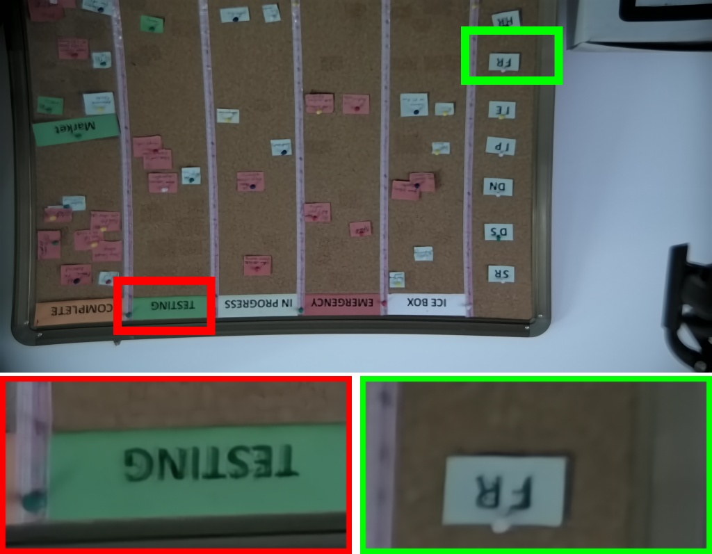
(g) MPRNet*

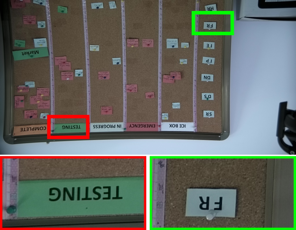
(h) GT

Figure 16: Visual comparison between different methods on SDD dataset.

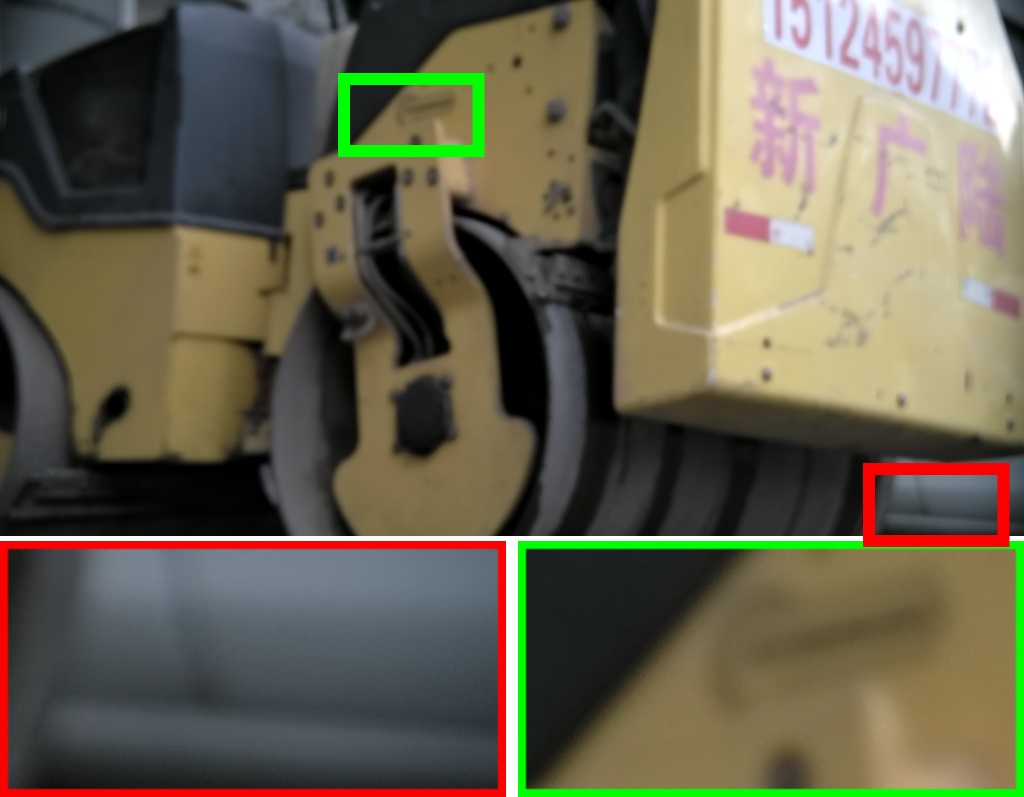
(a) Input

(b) UNet

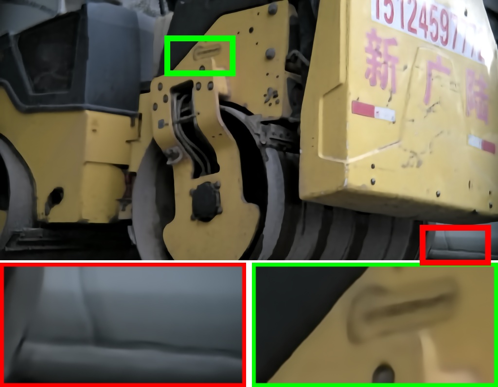
(c) MPRNet

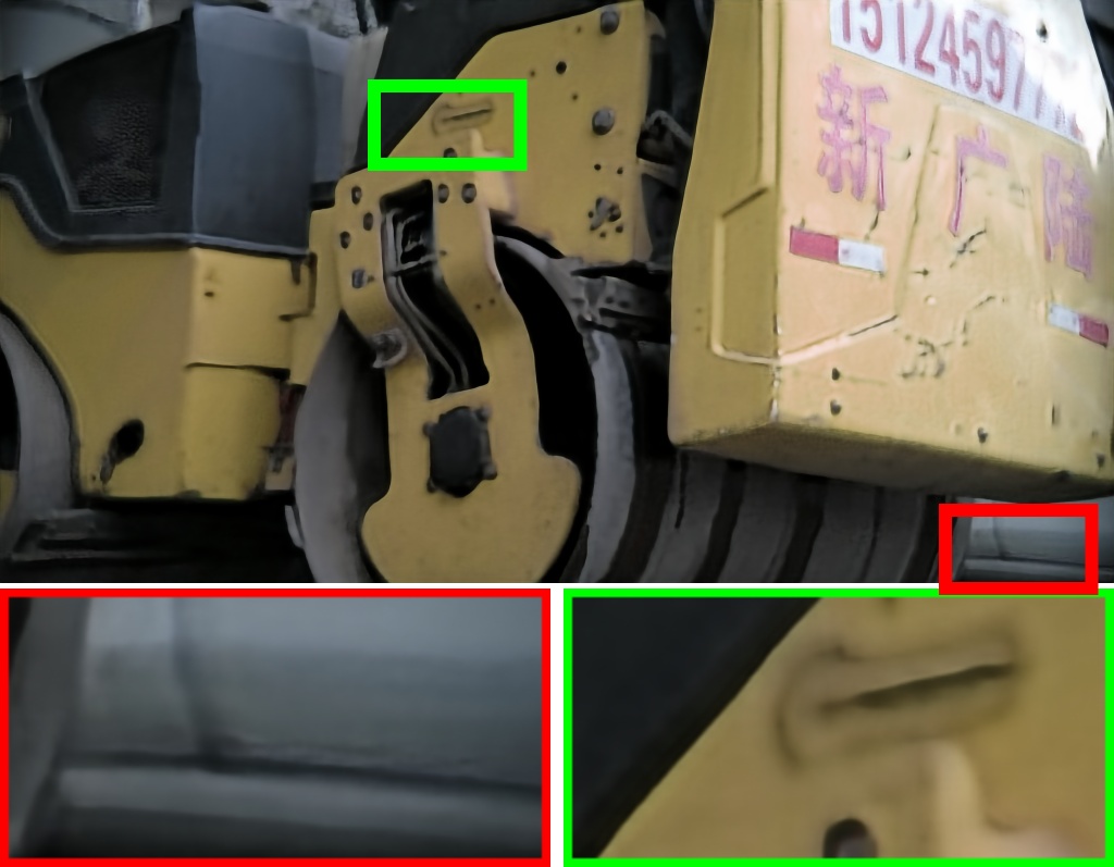
(d) DPDNet_S

(e) DMPHN

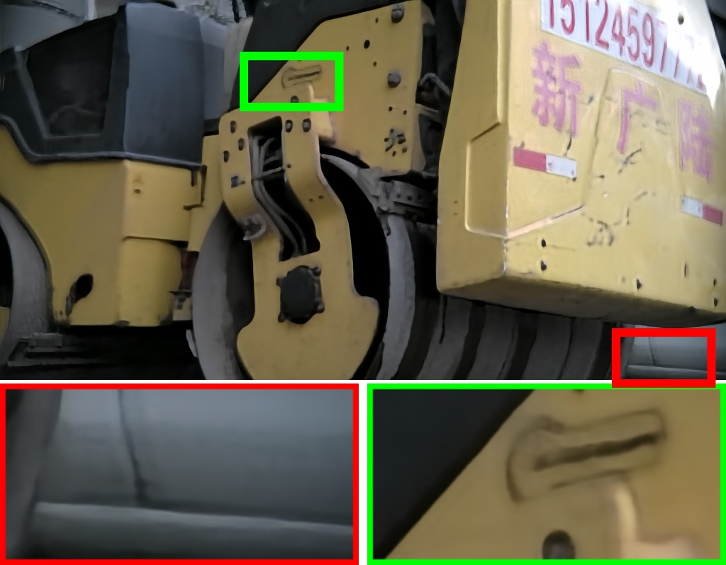
(f) UNet*

(g) MPRNet*

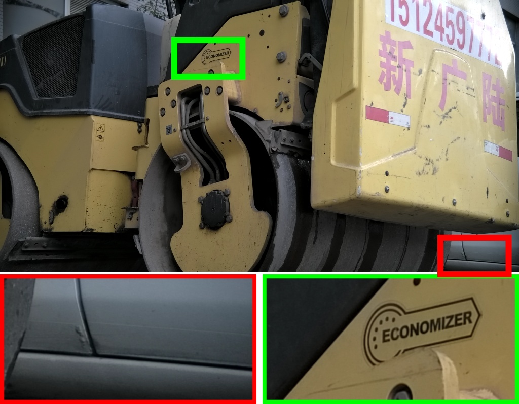
(h) GT

Figure 17: Visual comparison between different methods on SDD dataset.

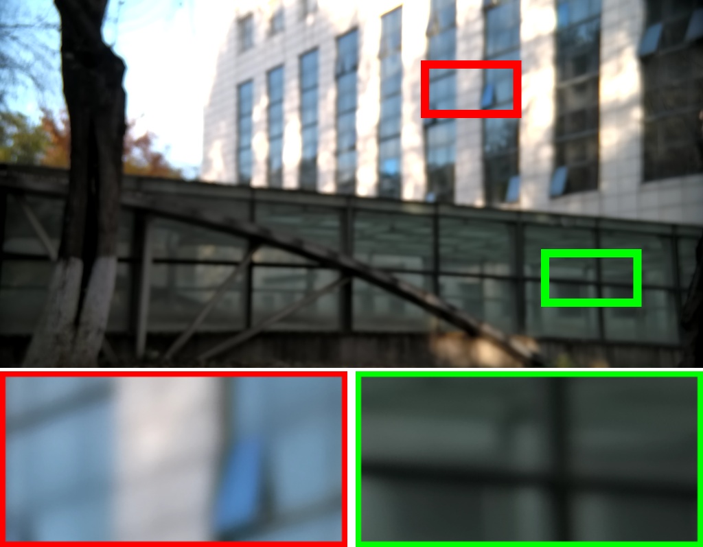
(a) Input

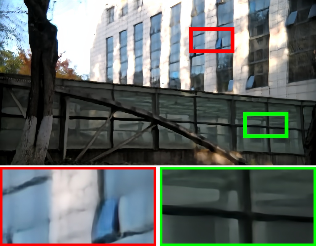
(b) UNet

(c) MPRNet

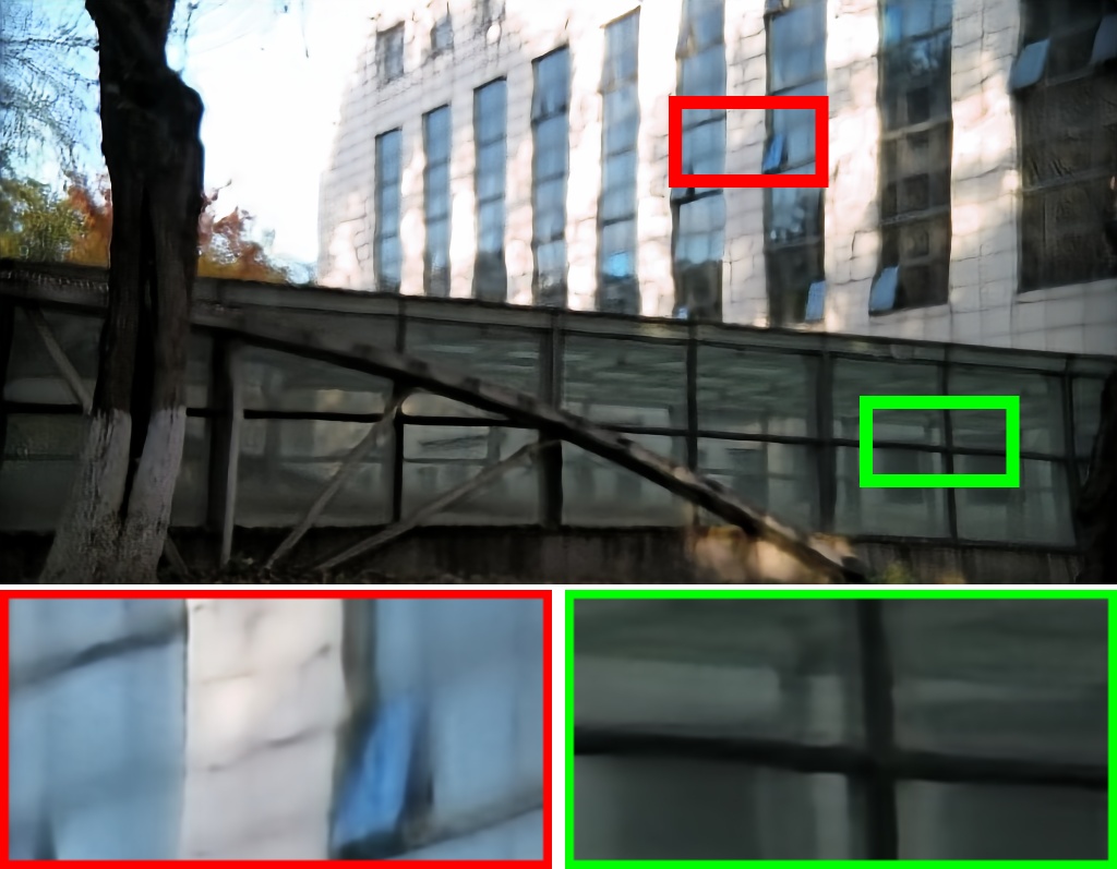
(d) DPDNet_S

(e) DMPHN

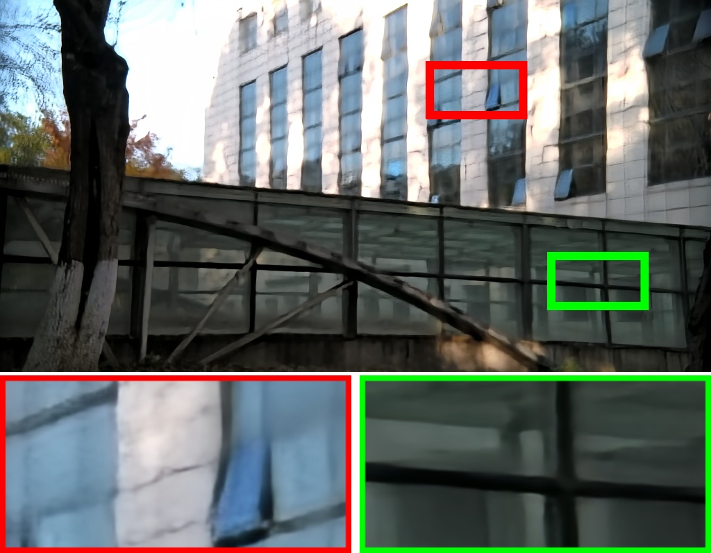
(f) UNet*

(g) MPRNet*

(h) GT

Figure 18: Visual comparison between different methods on SDD dataset.

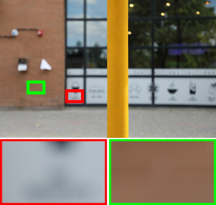
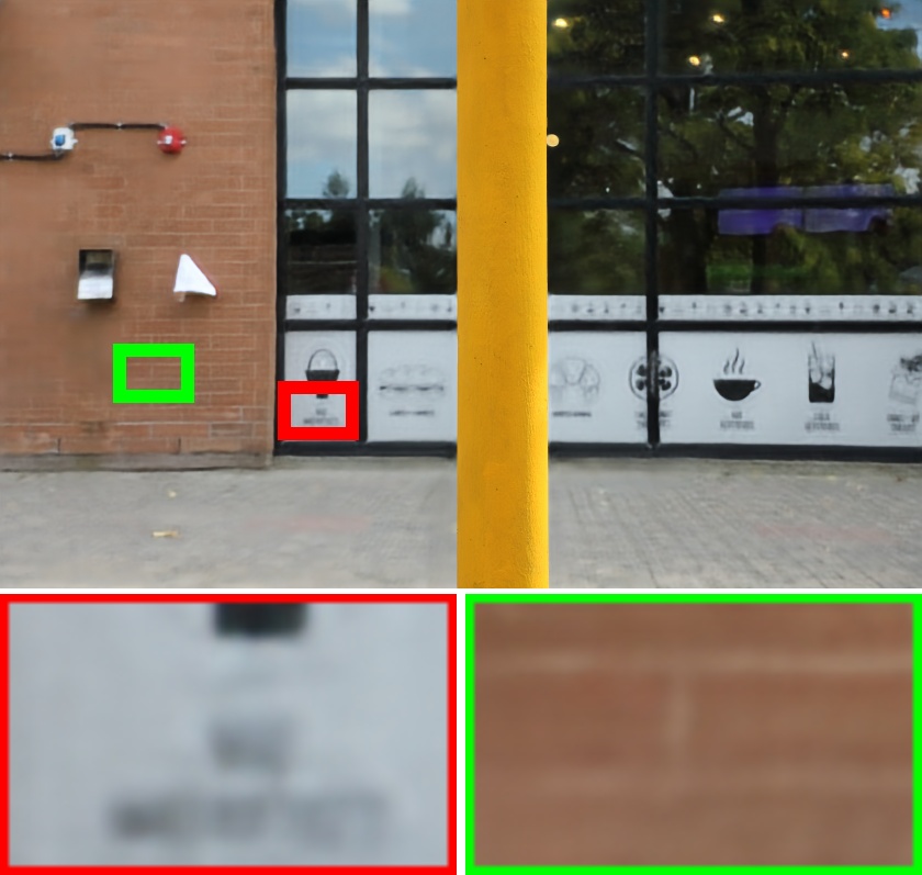
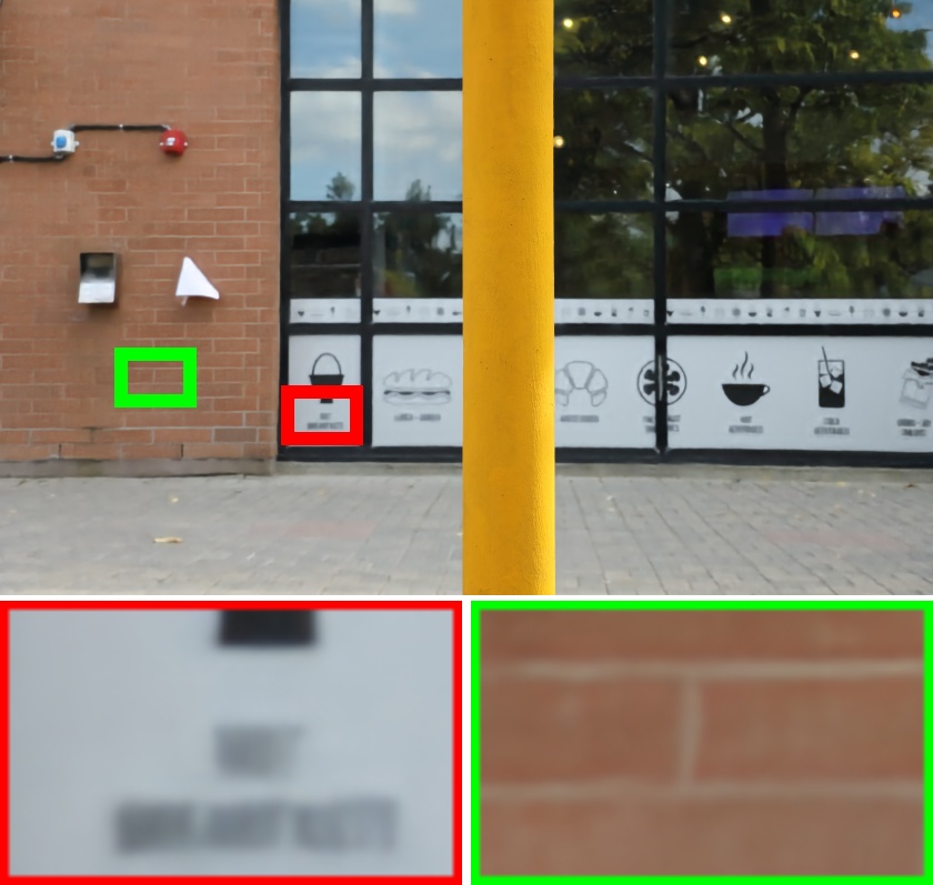
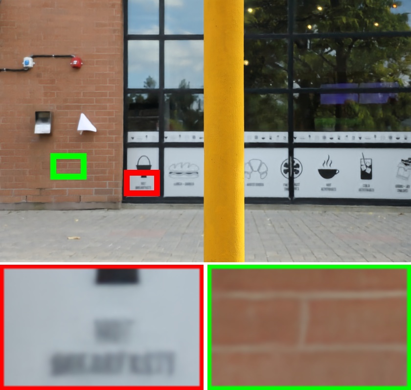
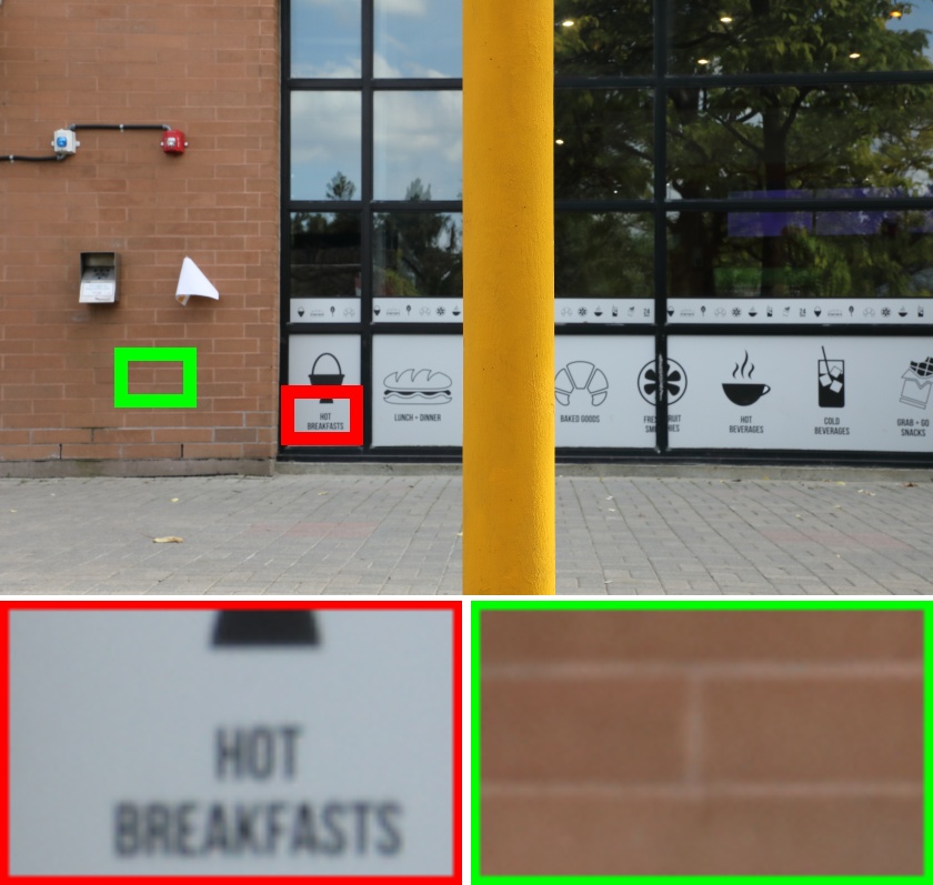
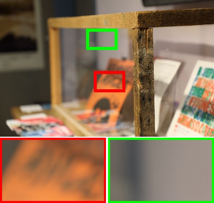
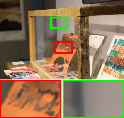
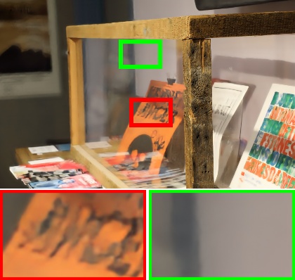
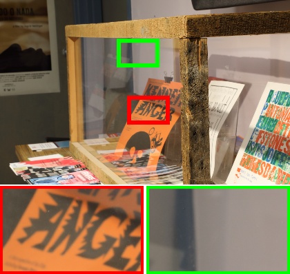
Input	UNet	UNet*	MPRNet	MPRNet*	GT

(a) Visual comparison between different methods on DPDD dataset.

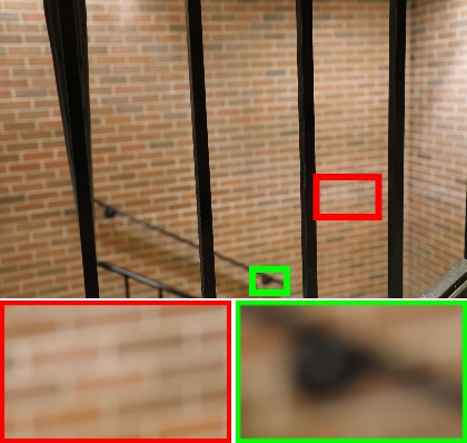
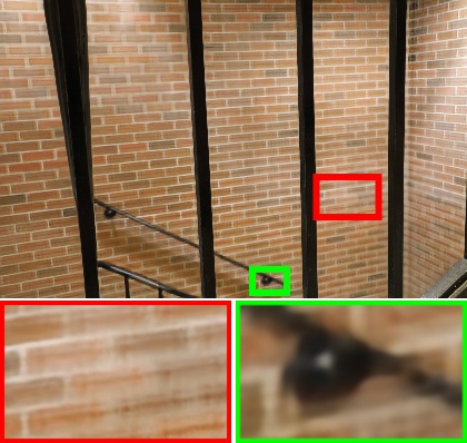
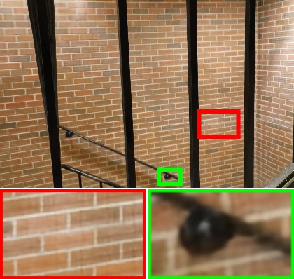
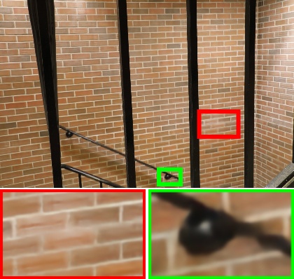
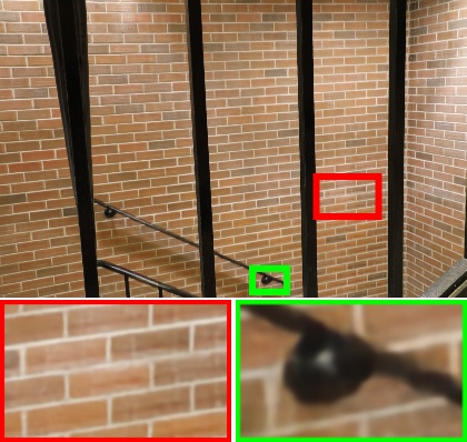
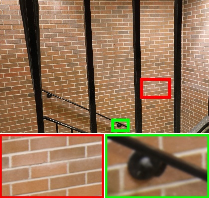
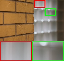
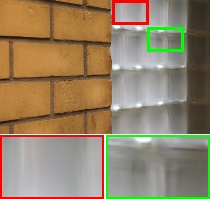
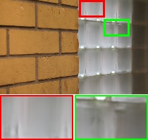
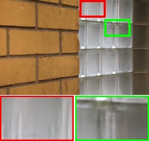
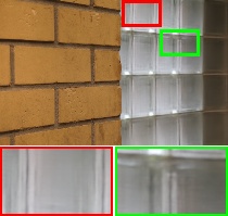
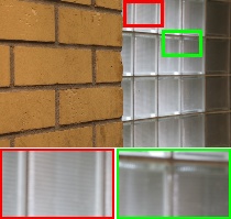
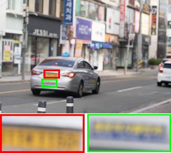
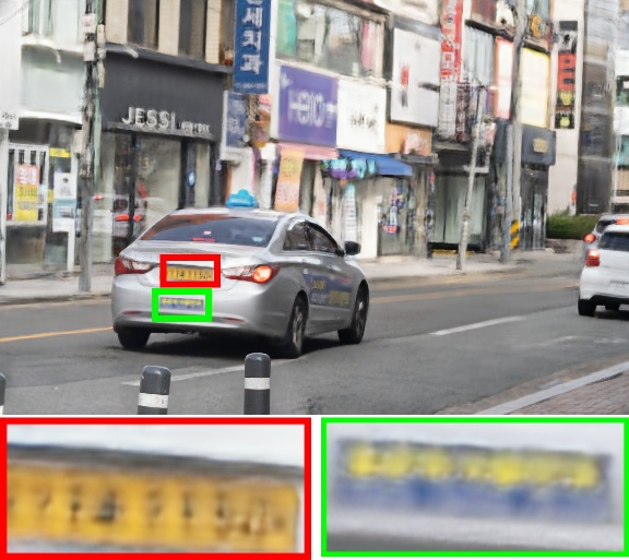
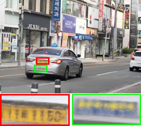
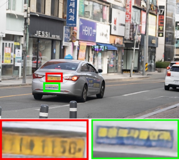
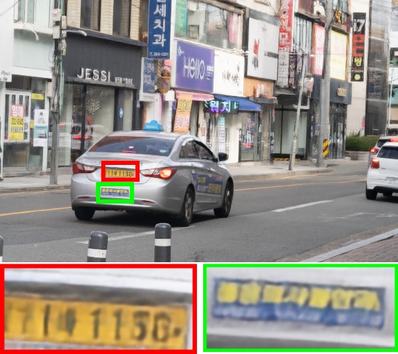
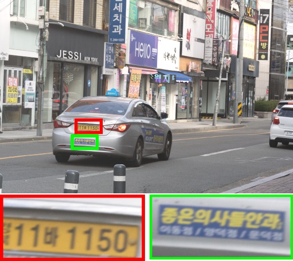
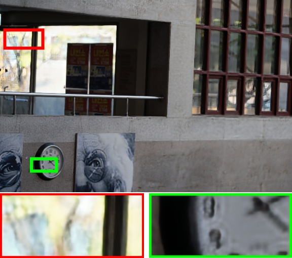
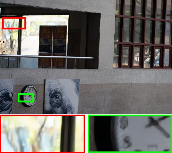
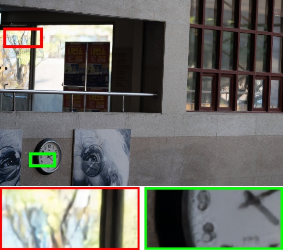
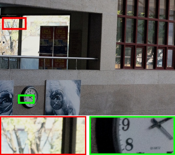
Input	DPDNetS	Son et al.	IFAN	IFAN*	GT

(b) Visual comparison between different methods on DPDD and RealDOF datasets. The first two rows are from DPDD and the last two rows are from RealDOF.

Figure 19: Visual results on DPDD and RealDOF dataset.

References

- Abuolaim and Brown (2020) Abuolaim, A.; and Brown, M. S. 2020. Defocus Deblurring Using Dual-Pixel Data. In European Conference on Computer Vision, 111–126. Springer.
- Abuolaim et al. (2021) Abuolaim, A.; Delbracio, M.; Kelly, D.; Brown, M. S.; and Milanfar, P. 2021. Learning to Reduce Defocus Blur by Realistically Modeling Dual-Pixel Data. In Proceedings of the IEEE/CVF International Conference on Computer Vision, 2289–2298.
- Charbonnier et al. (1994) Charbonnier, P.; Blanc-Feraud, L.; Aubert, G.; and Barlaud, M. 1994. Two deterministic half-quadratic regularization algorithms for computed imaging. In Proceedings of 1st International Conference on Image Processing, volume 2, 168–172. IEEE.
- Cun and Pun (2020) Cun, X.; and Pun, C.-M. 2020. Defocus blur detection via depth distillation. In European Conference on Computer Vision, 747–763. Springer.
- DAndrs et al. (2016) DAndrs, L.; Salvador, J.; Kochale, A.; and Süsstrunk, S. 2016. Non-parametric blur map regression for depth of field extension. IEEE Transactions on Image Processing, 25(4): 1660–1673.
- DP and Ba (2015) DP, K.; and Ba, J. 2015. Adam: A method for stochastic optimization. In Proc. of the 3rd International Conference for Learning Representations (ICLR).
- Fish et al. (1995) Fish, D.; Brinicombe, A.; Pike, E.; and Walker, J. 1995. Blind deconvolution by means of the Richardson–Lucy algorithm. JOSA A, 12(1): 58–65.
- He et al. (2015) He, K.; Zhang, X.; Ren, S.; and Sun, J. 2015. Delving deep into rectifiers: Surpassing human-level performance on imagenet classification. In Proceedings of the IEEE International Conference on Computer Vision, 1026–1034.
- Herrmann et al. (2020) Herrmann, C.; Bowen, R. S.; Wadhwa, N.; Garg, R.; He, Q.; Barron, J. T.; and Zabih, R. 2020. Learning to Autofocus. In Proceedings of the IEEE/CVF Conference on Computer Vision and Pattern Recognition (CVPR), 2230–2239.
- Karaali and Jung (2017) Karaali, A.; and Jung, C. R. 2017. Edge-based defocus blur estimation with adaptive scale selection. IEEE Transactions on Image Processing, 27(3): 1126–1137.
- Kong et al. (2020) Kong, T.; Sun, F.; Liu, H.; Jiang, Y.; Li, L.; and Shi, J. 2020. Foveabox: Beyound anchor-based object detection. IEEE Transactions on Image Processing, 29: 7389–7398.
- Krishnan and Fergus (2009) Krishnan, D.; and Fergus, R. 2009. Fast image deconvolution using hyper-Laplacian priors. Advances in Neural Information Processing Systems, 22: 1033–1041.
- Lee et al. (2019) Lee, J.; Lee, S.; Cho, S.; and Lee, S. 2019. Deep Defocus Map Estimation Using Domain Adaptation. In Proceedings of the IEEE/CVF Conference on Computer Vision and Pattern Recognition (CVPR), 12222–12230.
- Lee et al. (2021) Lee, J.; Son, H.; Rim, J.; Cho, S.; and Lee, S. 2021. Iterative filter adaptive network for single image defocus deblurring. In Proceedings of the IEEE/CVF Conference on Computer Vision and Pattern Recognition, 2034–2042.
- Pan et al. (2021) Pan, L.; Chowdhury, S.; Hartley, R.; Liu, M.; Zhang, H.; and Li, H. 2021. Dual Pixel Exploration: Simultaneous Depth Estimation and Image Restoration. In Proceedings of the IEEE/CVF Conference on Computer Vision and Pattern Recognition (CVPR), 4340–4349.
- Park et al. (2017) Park, J.; Tai, Y.-W.; Cho, D.; and So Kweon, I. 2017. A Unified Approach of Multi-Scale Deep and Hand-Crafted Features for Defocus Estimation. In Proceedings of the IEEE Conference on Computer Vision and Pattern Recognition (CVPR), 1736–1745.
- Paszke et al. (2019) Paszke, A.; Gross, S.; Massa, F.; Lerer, A.; Bradbury, J.; Chanan, G.; Killeen, T.; Lin, Z.; Gimelshein, N.; Antiga, L.; et al. 2019. Pytorch: An imperative style, high-performance deep learning library. Advances in Neural Information Processing Systems, 32: 8026–8037.
- Rim et al. (2020) Rim, J.; Lee, H.; Won, J.; and Cho, S. 2020. Real-world blur dataset for learning and benchmarking deblurring algorithms. In European Conference on Computer Vision, 184–201. Springer.
- Ronneberger, Fischer, and Brox (2015) Ronneberger, O.; Fischer, P.; and Brox, T. 2015. U-net: Convolutional networks for biomedical image segmentation. In International Conference on Medical Image Computing and Computer-assisted Intervention, 234–241. Springer.
- Ruan et al. (2022) Ruan, L.; Chen, B.; Li, J.; and Lam, M. 2022. Learning to Deblur using Light Field Generated and Real Defocus Images. In Proceedings of the IEEE/CVF Conference on Computer Vision and Pattern Recognition, 16304–16313.
- Shi, Xu, and Jia (2014) Shi, J.; Xu, L.; and Jia, J. 2014. Discriminative blur detection features. In Proceedings of the IEEE Conference on Computer Vision and Pattern Recognition, 2965–2972.
- Shi, Xu, and Jia (2015) Shi, J.; Xu, L.; and Jia, J. 2015. Just Noticeable Defocus Blur Detection and Estimation. In Proceedings of the IEEE Conference on Computer Vision and Pattern Recognition (CVPR), 657–665.
- Śliwiński and Wachel (2013) Śliwiński, P.; and Wachel, P. 2013. A simple model for on-sensor phase-detection autofocusing algorithm. Journal of Computer and Communications, 1(06): 11.
- Son et al. (2021) Son, H.; Lee, J.; Cho, S.; and Lee, S. 2021. Single image defocus deblurring using kernel-sharing parallel atrous convolutions. In Proceedings of the IEEE/CVF International Conference on Computer Vision, 2642–2650.
- Sun et al. (2018) Sun, D.; Yang, X.; Liu, M.-Y.; and Kautz, J. 2018. Pwc-net: Cnns for optical flow using pyramid, warping, and cost volume. In Proceedings of the IEEE conference on computer vision and pattern recognition, 8934–8943.
- Sun et al. (2022) Sun, P.; Cao, J.; Jiang, Y.; Yuan, Z.; Bai, S.; Kitani, K.; and Luo, P. 2022. DanceTrack: Multi-Object Tracking in Uniform Appearance and Diverse Motion. In Proceedings of the IEEE/CVF Conference on Computer Vision and Pattern Recognition (CVPR), 20993–21002.
- Tang et al. (2019) Tang, C.; Zhu, X.; Liu, X.; Wang, L.; and Zomaya, A. 2019. Defusionnet: Defocus blur detection via recurrently fusing and refining multi-scale deep features. In Proceedings of the IEEE/CVF Conference on Computer Vision and Pattern Recognition, 2700–2709.
- Wang et al. (2004) Wang, Z.; Bovik, A. C.; Sheikh, H. R.; and Simoncelli, E. P. 2004. Image quality assessment: from error visibility to structural similarity. IEEE Transactions on Image Processing, 13(4): 600–612.
- Xin et al. (2021) Xin, S.; Wadhwa, N.; Xue, T.; Barron, J. T.; Srinivasan, P. P.; Chen, J.; Gkioulekas, I.; and Garg, R. 2021. Defocus Map Estimation and Deblurring from a Single Dual-Pixel Image. In Proceedings of the IEEE/CVF International Conference on Computer Vision, 2228–2238.
- Yi and Eramian (2016) Yi, X.; and Eramian, M. 2016. LBP-based segmentation of defocus blur. IEEE Transactions on Image Processing, 25(4): 1626–1638.
- Zamir et al. (2021) Zamir, S. W.; Arora, A.; Khan, S.; Hayat, M.; Khan, F. S.; Yang, M.-H.; and Shao, L. 2021. Multi-stage progressive image restoration. In Proceedings of the IEEE/CVF Conference on Computer Vision and Pattern Recognition, 14821–14831.
- Zhang et al. (2019) Zhang, H.; Dai, Y.; Li, H.; and Koniusz, P. 2019. Deep stacked hierarchical multi-patch network for image deblurring. In Proceedings of the IEEE/CVF Conference on Computer Vision and Pattern Recognition, 5978–5986.
- Zhang et al. (2022) Zhang, K.; Wang, T.; Luo, W.; Chen, B.; Ren, W.; Stenger, B.; Liu, W.; Li, H.; and Ming-Hsuan, Y. 2022. MC-Blur: A Comprehensive Benchmark for Image Deblurring. In arXiv:2112.00234.
- Zhang et al. (2018) Zhang, R.; Isola, P.; Efros, A. A.; Shechtman, E.; and Wang, O. 2018. The unreasonable effectiveness of deep features as a perceptual metric. In Proceedings of the IEEE Conference on Computer Vision and Pattern Recognition, 586–595.
- Zhao et al. (2018) Zhao, W.; Zhao, F.; Wang, D.; and Lu, H. 2018. Defocus blur detection via multi-stream bottom-top-bottom fully convolutional network. In Proceedings of the IEEE conference on computer vision and pattern recognition, 3080–3088.
- Zheng et al. (2022) Zheng, Y.; Duan, Y.; Lu, J.; Zhou, J.; and Tian, Q. 2022. HyperDet3D: Learning a Scene-Conditioned 3D Object Detector. In Proceedings of the IEEE/CVF Conference on Computer Vision and Pattern Recognition (CVPR), 5585–5594.

References

- Zhang et al. (2019b) Zhang, X.; Chen, Q.; Ng, R.; and Koltun, V. 2019b. Zoom to learn, learn to zoom. In Proceedings of the IEEE/CVF Conference on Computer Vision and Pattern Recognition, 3762–3770.
- Kong et al. (2021) Kong, L.; Lian, C.; Huang, D.; Hu, Y.; Zhou, Q.; et al. 2021. Breaking the dilemma of medical image-to-image translation. Advances in Neural Information Processing Systems, 34: 1964–1978.
- Zhu et al. (2017) Zhu, J.-Y.; Park, T.; Isola, P.; and Efros, A. A. 2017. Unpaired image-to-image translation using cycle-consistent adversarial networks. In Proceedings of the IEEE international conference on computer vision, 2223–2232.