Comparison Between Mean-Variance and Monotone Mean-Variance Preferences Under Jump Diffusion and Stochastic Factor Model

Abstract

This paper compares the optimal investment problems based on monotone mean-variance (MMV) and mean-variance (MV) preferences in the Lévy market with an untradable stochastic factor. It is an open question proposed by Trybuła and Zawisza. Using the dynamic programming and Lagrange multiplier methods, we get the HJBI and HJB equations corresponding to the two investment problems. The equations are transformed into a new-type parabolic equation, from which the optimal strategies under both preferences are derived. We prove that the two optimal strategies and value functions coincide if and only if an important market assumption holds. When the assumption violates, MMV investors act differently from MV investors. Thus, we conclude that the difference between continuous-time MMV and MV portfolio selections is due to the discontinuity of the market. In addition, we derive the efficient frontier and analyze the economic impact of the jump diffusion risky asset. We also provide empirical evidences to demonstrate the validity of the assumption in real financial market.

Keywords: stochastic control; monotone mean-variance preferences; stochastic factor; Lévy market; optimal investment

1 Introduction.

Since Markowits (1952) proposed the mean-variance preference, it became a popular criterion in portfolio selection problems. Previous works have widely considered both multi-period discrete and continuous-time portfolio selection problems under mean-variance preferences. Li and Ng (2000) and Zhou and Li (2000) use embedding techniques to overcome the time-inconsistency of mean-variance preferences, leading a great number of following works, see e.g., Černỳ and Kallsen (2007), Li et al. (2002), Lim and Zhou (2002) and Lim (2004). However, when we consider the optimal investment problems, there is still another drawback of mean-variance preferences: non-monotonicity.

For a preference $\rho$ with monotonicity, if two random variables satisfy $X\leqslant Y$ almost surely, we expect $\rho(X)\leqslant\rho(Y)$. However, mean-variance preferences do not have such property. A strictly wealthier investor may have a lower utility than others, which violates the basic assumption of economic rationality. Maccheroni et al. (2009) provide an example to illustrate the non-monotonicity of mean-variance preferences. To conquer such a disadvantage, they propose a new criterion named the monotone mean-variance preference. It is the best possible monotone approximation of the classical mean-variance preference without loss of good tractability. In this paper, we use the abbreviations MMV and MV to denote monotone mean-variances and mean-variances.

There are several works related to MMV preferences. Trybuła and Zawisza (2019) study the optimal investment problem in a continuous-time financial market model with a stochastic factor. Using the method of dynamic programming and solving the Hamilton–Jacobi–Bellman–Isaacs (HJBI) equation, they propose a verification theorem and obtain an explicit optimal strategy of the investment under MMV preferences. Trybuła and Zawisza (2019) use the result from Zawisza (2012) and prove that the optimal strategies under MMV and MV preferences are the same, which is different from the conclusion of the single-period case considered in Maccheroni et al. (2009). The reason of this difference may be either the discreteness or the discontinuity of the wealth process. Using the analytic approach rather than comparing the two optimal strategies directly, Strub and Li (2020) generalize the conclusion of Trybuła and Zawisza (2019) to all continuous semimartingale financial market models. In the continuous market scenario, Li and Guo (2021) solve the optimal reinsurance and investment problem in a multidimensional diffusion model, using the same HJBI approach as Mataramvura and Øksendal (2008) and Trybuła and Zawisza (2019). Recently, there are also works studying MMV investment problems when the trading strategy is constrained, see e.g., Shen and Zou (2022), Hu et al. (2023) and Du and Strub (2023). They all conclude that the solutions to MMV and MV problems coincide when the asset is continuous.

As the method and result of Strub and Li (2020) can only be applied to continuous markets, a crucial question is whether the conclusion still holds true in any Lévy market. It is also an open question raised by Trybuła and Zawisza (2019) for further study. Thus, to find the relationship between the two optimal strategies under MMV and MV preferences in the Lévy market, we consider a jump diffusion financial market. Besides, an untradable stochastic factor is also included in our model for two reasons. First, if we follow the model setup of Trybuła and Zawisza (2019), then we can compare our result with the former work and the difference is the pure effect of the jump risk. Second, markets with stochastic factors are incomplete. Bäuerle and Grether (2015) propose a detailed definition of the free cash flow stream and prove that there is no free cash flow stream in any complete and arbitrage-free market. That is why the optimal strategy of an MV investor would never escape the monotone domain of MV preferences in such market. Therefore, it is necessary to consider an incomplete market in our research. It is important to note that the jump diffusion part of our model can also lead to the incomplete property of the market, depending on the specific coefficient setting of the jump strength.

From another perspective, we can regard the MMV preference as a robust utility, which is considered in many robust optimization problems, e.g., Gilboa and Schmeidler (1989), Zawisza (2010) and Øksendal and Sulem (2014). In a jump diffusion model, Mataramvura and Øksendal (2008) consider such kind of max-min problem as a stochastic differential game. An interesting characterization on the set of ambiguity probability measures is proved in Li and Guo (2021), which helps us understand the range of ambiguity probability measures of MMV preferences even in the jump diffusion market. We will discuss more about this in Remark 1. In this paper, we mainly refer to Mataramvura and Øksendal (2008) and take a similar dynamic programming method to solve the MMV optimal investment problem in our market model.

Beside the non-monotonicity, another huge drawback of MV preferences is the time-inconsistency. The main reason for the time-inconsistency is the variance term in MV preferences, which yields the in-applicability of the dynamic programming method. Bjork and Murgoci (2010) propose a general theory of Markovian time inconsistent stochastic control problems, in which three approaches are raised to fix the time-inconsistency and find the optimal control. The first is to choose whatever seems to be optimal based on the investor’s current preference, without knowing the fact that his preference may change over time. The second is to find a pre-commitment solution, which means that the investor only considers the optimal problem once at the initial time and keeps taking that strategy all the time. All of the literature on MV preferences mentioned above actually uses the pre-commitment approach. The third is to define a new equilibrium solution and use game theory terms to formulate the problem. For example, Bjork and Murgoci (2010) find an equilibrium solution to the general utility form that includes MV preferences. Zeng et al. (2013) derive the optimal strategy of reinsurance and investment that holds time-consistency for MV insurers. All three approaches can be reasonable in different circumstances, depending on the goal of the study. In our paper, similar to Trybuła and Zawisza (2019), we use the pre-commitment approach, which is the best situation for us to analyze the relationship between MMV and MV problems. As we find that the optimal strategy under MMV preferences depend on the investor’s wealth and the market state, MMV preferences also have the time-inconsistency property as MV preferences.

The main contributions of our work are as follows. We refine the optimal investment problems with respect to MMV and MV preferences in a jump diffusion and stochastic factor model. To the best of our knowledge, this is the first time that these two preferences are considered in such a financial market model with jumps. We obtain the explicit optimal strategies of MMV and MV problems under certain assumptions (Conditions of Proposition 1 and Assumption 1). We prove that the two optimal strategies and value functions coincide if and only if Assumption 1 holds. Thus, the discontinuity of the market model may cause investors with MMV preferences to choose a different strategy from those with MV preferences. We answer the open question proposed by Trybuła and Zawisza (2019) and extend the conclusion of Strub and Li (2020). This phenomenon is interesting because it contradicts the consistency in continuous markets, where the two preferences are shown to yield the same result. Besides, under Assumption 1, we prove that the achieved maximum utilities of MMV and MV preferences are also the same, which is somehow ignored by Trybuła and Zawisza (2019). Theoretically, Assumption 1 may not hold, leading to the inconsistency of MMV and MV problems. Nevertheless, we also provide some empirical evidences to illustrate the validity of Assumption 1 in real financial market.

More specifically, we introduce the Doléans-Dade exponentials to replace the target probability measures of MMV preferences. In the MMV problem, we transform the problem into a stochastic differential game and use the dynamic programming method to obtain the HJBI equation. In the MV problem, we deal with the nonlinearity of the variance term first, and then obtain the HJB equation by combining the Lagrange multiplier and dynamic programming methods. To solve the HJBI and HJB equations, we obtain a new type of highly nonlinear parabolic partial differential equation. The equation cannot be simply transformed to a linear parabolic equation by the traditional Hopf-Cole transformation method used in Zariphopoulou (2001), Zawisza (2010) and Trybuła and Zawisza (2019). Instead, we refer to a new type existence and uniqueness theorem on parabolic equations from Ladyzhenskaya et al. (1968) to prove the existence and uniqueness of the solutions to HJBI and HJB equations. Then, we propose a jump diffusion type Feynman-Kac formula to prove the consistency of the two optimal strategies of MMV and MV problems under Assumption 1. Finally, we prove that the optimal strategies and value functions of MMV and MV problem are the same if and only if Assumption 1 holds. We also derive the efficient frontier of the investment and analyze the economic impact caused by the jump diffusion part of the risky asset.

The remainder of this paper is organized as follows. Section 2 introduces the market model and monotone mean-variance preferences. Section 3 solves the optimal investment problem with respect to MMV preferences. We formulate the HJBI equation and find the corresponding solution. Section 4 solves the optimal investment problem with respect to MV preferences. In Section 5, we compare the two optimal strategies and value functions and provide the sufficient and necessary condition for them to be consistent. Besides, we derive the efficient frontier and make some economic explanations. We also provide empirical evidences to demonstrate the validity of the assumption in real financial market. Finally, Section 6 concludes the paper.

2 Market model and MMV preference.

We consider a filtered probability space $\left(\Omega;\mathcal{F};\{\mathcal{F}_{t}\}_{t\geqslant 0};\mathbb{P}\right)$ satisfying the usual conditions. $W^{1}=\{W^{1}_{t},t\in[0,T]\}$ and $W^{2}=\{W^{2}_{t},t\in[0,T]\}$ are Brownian motions. ${N}$ is a Poisson random measure on $\left([0,T]\times\mathbb{R},\mathcal{B}([0,T]\times\mathbb{R})\right)$ with respect to a Lévy process $L$. Filtration $\{\mathcal{F}_{t}\}_{t\geqslant 0}$ is generated by $W^{1}$, $W^{2}$ and $N$. We assume that $W^{1}$, $W^{2}$ and $N$ are independent. Further more, we denote $\mathrm{d}t\nu(\mathrm{d}p)$ as the compensator (or intensity measure), and $\tilde{N}$ as the corresponding compensated martingale measure of $N$, i.e., $\tilde{N}\left(\mathrm{d}t,\mathrm{d}p\right)=N\left(\mathrm{d}t,\mathrm{d}p\right)-\mathrm{d}t\nu(\mathrm{d}p)$. We assume that $\nu(\mathbb{R})<+\infty$. For more information about the Poisson random measure, see Protter (2005) and Tankov (2003).

Suppose that there are two investment assets. The price process of the risk-free asset $B=\{B_{t},t\in[0,T]\}$ is given by

$$\mathrm{d}B_{t}=B_{t}r\mathrm{d}t,\ B_{0}=s_{0}.$$ (1)

And the risky asset $S=\{S_{t},t\in[0,T]\}$ follows a Lévy-Itö process, satisfying the following stochastic differential equation (SDE):

$$\mathrm{d}S_{t}=S_{t-}\left[\mu\left(Z_{t}\right)\mathrm{d}t+\sigma\left(Z_{t}\right)\mathrm{d}W^{1}_{t}+\int_{\mathbb{R}}\gamma\left(Z_{t},p\right)\tilde{N}\left(\mathrm{d}t,\mathrm{d}p\right)\right],\ S_{0}=s,$$ (2)

where the stochastic factor $Z=\{Z_{t},t\in[0,T]\}$ follows SDE:

$$\mathrm{d}Z_{t}=a\left(Z_{t}\right)\mathrm{d}t+b\left(Z_{t}\right)\left(\rho_{W}\mathrm{d}W^{1}_{t}+\bar{\rho}_{W}\mathrm{d}W^{2}_{t}\right),\ Z_{0}=z.$$ (3)

Besides, we assume $\gamma>-1$ with $\int_{\mathbb{R}}\gamma(z,p)^{2}\nu(\mathrm{d}p)<\infty$, coefficients $\mu,\sigma,a$ and $b$ are continuous functions, $\gamma$ is continuous with respect to $z$, and they satisfy all the required regularity conditions to ensure that SDEs (2) and (3) have unique strong solutions. Let $\rho_{W}$ represent the correlation of Brownian motion parts of $S$ and $Z$ and $\rho_{W}^{2}+\bar{\rho}_{W}^{2}=1$.

In this paper, we compare the optimal investment strategies of investors under MMV preferences and MV preferences. Now, we introduce the MMV preferences first. Based on Maccheroni et al. (2009), the class of MMV preferences is defined by

$$V_{\theta}(X)=\inf_{\mathbb{Q}\in\mathcal{Q}_{0}}\{\mathbb{E}^{\mathbb{Q}}[X]+\frac{1}{2\theta}C\left(\mathbb{Q}|\mathbb{P}\right)\},$$

$$C\left(\mathbb{Q}|\mathbb{P}\right)=\mathbb{E}^{\mathbb{P}}\left[\left(\frac{\mathrm{d}\mathbb{Q}}{\mathrm{d}\mathbb{P}}\right)^{2}\right]-1,$$

where

$$\mathcal{Q}_{0}=\left\{\mathbb{Q}:\mathbb{Q}\ll\mathbb{P},\ \mathbb{E}^{\mathbb{P}}\left[\left(\frac{\mathrm{d}\mathbb{Q}}{\mathrm{d}\mathbb{P}}\right)^{2}\right]<+\infty\right\}.$$

Moreover, MMV preferences can be rewritten as

$$V_{\theta}(X)=-\Lambda_{\theta}(X)-\frac{1}{2\theta},$$

where

$$\Lambda_{\theta}(X)=\sup_{\mathbb{Q}\in\mathcal{Q}_{0}}\mathbb{E}^{\mathbb{Q}}\left[-X-\frac{1}{2\theta}\frac{\mathrm{d}\mathbb{Q}}{\mathrm{d}\mathbb{P}}\right].$$

For simplicity, we denote $\Lambda_{\theta}$ as the objective function used in the MMV investment problem.

Naturally, we consider the set of all the Doléans-Dade exponential measures

$$\mathcal{Q}=\left\{\mathbb{Q}^{\eta,\phi}\ll\mathbb{P}:\frac{\mathrm{d}\mathbb{Q}^{\eta,\phi}}{\mathrm{d}\mathbb{P}}=\mathcal{E}\left(\int\eta_{1,t}\mathrm{d}W^{1}_{t}+\int\eta_{2,t}\mathrm{d}W^{2}_{t}+\int\int_{\mathbb{R}}\phi_{t}(p)\tilde{N}\left(\mathrm{d}t,\mathrm{d}p\right)\right)_{T},(\eta,\phi)\in\mathcal{M}\right\},$$

to replace $\mathcal{Q}_{0}$, where the range of $(\eta,\phi)=(\eta_{1,t},\eta_{2,t},\phi_{t})_{0\leqslant t\leqslant T}$ is given by

$$\mathcal{M}=\left\{(\eta,\phi)\text{ is predictable}:\mathbb{E}^{\mathbb{P}}\left[\left(\frac{\mathrm{d}\mathbb{Q}^{\eta,\phi}}{\mathrm{d}\mathbb{P}}\right)^{2}\right]<\infty,\ \mathbb{E}^{\mathbb{P}}\left[\frac{\mathrm{d}\mathbb{Q}^{\eta,\phi}}{\mathrm{d}\mathbb{P}}\right]=1,\frac{\mathrm{d}\mathbb{Q}^{\eta,\phi}}{\mathrm{d}\mathbb{P}}\geqslant 0\right\}.$$

For $\mathbb{Q}\in\mathcal{Q}$, we just restrict it to satisfy $\mathbb{Q}\ll\mathbb{P}$ and $\frac{\mathrm{d}\mathbb{Q}}{\mathrm{d}\mathbb{P}}\geqslant 0$ rather than $\mathbb{Q}\sim\mathbb{P}$ as in Trybuła and Zawisza (2019). It is a notable difference, because we cannot ensure the target $\mathbb{Q}$ to be equivalent to $\mathbb{P}$ when the market faces jump risks. For the aim of clarity, we state the definition of the Doléans-Dade exponential and stress one of its important properties here.

Definition 1.

For a semimartingale $M$ with $M_{0}=0$, the stochastic exponential (Doléans-Dade exponential) of $M$, written as $\mathcal{E}(M)$, is the unique semimartingale $X$ satisfying

$$X_{t}=1+\int_{0}^{t}X_{s-}\mathrm{d}M_{s}.$$

Detailedly, $X$ can be represented by

$$X_{t}=\exp\left\{M_{t}-\frac{1}{2}\left[M,M\right]^{c}_{t}\right\}\prod_{0<s\leqslant t}(1+\Delta X_{s})\exp\big{\{}-\Delta X_{s}\big{\}},$$ (4)

where the infinite product converges and is càdlàg with finite variation.

For more information about the Doléans-Dade exponential, see Protter (2005), Section 8 of Chapter II. Furthermore, similar to the well-known Kazamaki’s and Novikov’s criteria, we need the following criterion to determine whether a Doléans-Dade exponential is a martingale and then $\mathbb{Q}^{\eta,\phi}$ to be a true probability measure.

Lemma 1 (Mémin’s criterion for exponential martingale).

Let $M$ be a local martingale and $M^{0}_{t}=\sum_{s\leqslant t}{\Delta M_{s}\mathbf{1}_{|\Delta M_{s}|\geqslant\frac{1}{2}}}$. Let $M^{1}_{t}$ be the compensator of $M^{0}_{t}$: $M^{1}_{t}=M^{0}_{t}-\tilde{M^{0}_{t}}$, and $M^{2}_{t}=M_{t}-M^{1}_{t}$. If the compensator of process

$$\left[M^{c},M^{c}\right]_{t}+\sum_{0<s\leqslant t}|\Delta M^{1}_{t}|+\sum_{0<s\leqslant t}\left(\Delta M^{2}_{t}\right)^{2}$$

is bounded, then $\mathcal{E}(M)$ is a uniformly integrable martingale.

Proof.

Proof. See Theorem III-3 in Mémin (2006) or Exercise 13 of Chapter V in Protter (2005). ∎

Now, we introduce a new process $Y^{\eta,\phi}=\{Y^{\eta,\phi}_{t},t\in[0,T]\}$ as follows:

$$\mathrm{d}Y_{s}^{\eta,\phi}=Y_{s-}^{\eta,\phi}\left[\eta_{1,s}\mathrm{d}W^{1}_{s}+\eta_{2,s}\mathrm{d}W^{2}_{s}+\int_{\mathbb{R}}\phi_{s}(p)\tilde{N}\left(\mathrm{d}s,\mathrm{d}p\right)\right],\ Y_{t}=y.$$ (5)

Based on the uniqueness of SDE’s solution, we have $Y_{T}^{\eta,\phi}=y\frac{\mathrm{d}\mathbb{Q}^{\eta,\phi}}{\mathrm{d}\mathbb{P}}$ when starting with $t=0$ and $Y_{0}=y$. If we set $y=\frac{1}{2\theta}$, the objective function restricted by the maximization on $\mathcal{Q}$ becomes

$$\Lambda_{\theta}(X)=\sup_{\mathbb{Q}^{\eta,\phi}\in\mathcal{Q}}\mathbb{E}^{\mathbb{Q}^{\eta,\phi}}\left[-X-Y_{T}^{\eta,\phi}\right].$$

Notably, when $y\neq 0$, $\frac{Y_{T}^{\eta,\phi}}{y}=\frac{\mathrm{d}\mathbb{Q}^{\eta,\phi}}{\mathrm{d}\mathbb{P}}$ should be greater than 0. Thus, not all the predictable $(\eta,\phi)$ meet the requirement. We consider a series of admissible sets of $(\eta,\phi)$:

$$\mathcal{M}^{t}=\Big{\{}(\eta,\phi)= (\eta_{1,s},\eta_{2,s},\phi_{s})_{t\leqslant s\leqslant T}\text{ is predictable}:\text{The solution of Equation \eqref{eq dynamic of Y} satisfies}$$

$$\mathbb{E}^{\mathbb{P}}\left[(Y_{T}^{\eta,\phi})^{2}\right]\leqslant+\infty,\mathbb{E}^{\mathbb{P}}\left[Y_{T}^{\eta,\phi}\right]=1,Y_{T}^{\eta,\phi}\geqslant 0,\text{ for }\forall y>0\Big{\}},\ 0\leqslant t\leqslant T.$$

Denote $\mathcal{Q}^{t}$ as the set of all the Doléans-Dade exponential measures with respect to $\mathcal{M}^{t}$. It is trivial to see that $\mathcal{M}^{0}=\mathcal{M}$ and $\mathcal{Q}^{0}=\mathcal{Q}$. Further, we denote $\mathbb{E}^{\mathbb{Q}^{\eta,\phi}}$ by $\mathbb{E}^{\eta,\phi}$ for simplicity. In the following discussion, we restrict the maximization (minimization) over $\mathbb{Q}$ on $\mathcal{Q}^{t}$ in the definition of $\Lambda_{\theta}$ ($V_{\theta}$), unless otherwise noted. See Remark 1 for more detailed explanations.

Remark 1.

In fact, the Doléans-Dade exponential may not exhaust all the probability measure $\mathbb{Q}$ in $\mathcal{Q}_{0}$, which means $\mathcal{Q}^{t}\subset\mathcal{Q}_{0}$. Two reasons support us to consider $\mathcal{Q}^{t}$ as the target probability set. First, we will prove in Section 5 that under certain conditions, the optimal control and value function of the MMV problem would be consistent no matter $\mathcal{Q}^{t}$ or $\mathcal{Q}_{0}$ is considered. Second, Li and Guo (2021) propose that any $\mathbb{Q}$ in $\mathcal{Q}_{0}$ is indeed a Doléans-Dade exponential if we consider $\{\mathcal{F}_{t}\}_{t\geqslant 0}$ as the filtration generated by Brownian motions, and $\mathbb{Q}$ as all the Doléans-Dade exponential measures generated by Brownian motions. It inspires us to consider such form of probability measures even in the jump diffusion financial market.

3 MMV problem.

In this section, we solve the optimal investment problem under MMV preferences. We treat the max-min optimization problem as a stochastic differential game between an investor and a potential market player. We use the dynamic programming method to get the HJBI equation and propose a verification theorem. The optimal investment strategy is then obtained by solving the HJBI equation and verifying the verification theorem.

First, we introduce the investor’s wealth process. Let $\bar{\pi}=\{\bar{\pi}_{t},t\in[0,T]\}$ be the process of investment amount in the risky asset. Then, the wealth process $\bar{X}$ satisfies the following SDE:

$$\left\{\begin{aligned} &\mathrm{d}\bar{X}_{t}^{\bar{\pi}}=\bar{X}_{t}^{\bar{\pi}}r\mathrm{d}t+\bar{\pi}_{t}\left(\mu\left(Z_{t}\right)-r\right)\mathrm{d}t+\bar{\pi}_{t}\sigma\left(Z_{t}\right)\mathrm{d}W^{1}_{t}+\bar{\pi}_{t}\int_{\mathbb{R}}\gamma\left(Z_{t},p\right)\tilde{N}\left(\mathrm{d}t,\mathrm{d}p\right),\\ &X_{0}=x.\end{aligned}\right.$$

Similar to Trybuła and Zawisza (2019), we consider $\pi=\{e^{r(T-t)}\bar{\pi}_{t},t\in[0,T]\}$ and $X^{{\pi}}=\{e^{r(T-t)}\bar{X}_{t}^{\bar{\pi}},t\in[0,T]\}$ as the forward value processes of the investment amount and wealth for simplicity. Then, the wealth process of the self-financed investor satisfies:

$$\left\{\begin{aligned} &\mathrm{d}X_{t}^{\pi}=\pi_{t}\left(\mu\left(Z_{t}\right)-r\right)\mathrm{d}t+\pi_{t}\sigma\left(Z_{t}\right)\mathrm{d}W^{1}_{t}+\pi_{t}\int_{\mathbb{R}}\gamma\left(Z_{t},p\right)\tilde{N}\left(\mathrm{d}t,\mathrm{d}p\right),\\ &X_{0}=x.\end{aligned}\right.$$ (6)

Definition 2.

An investment strategy $\pi=\{\pi_{s}\}_{t\leqslant s\leqslant T}$ is admissible $(\pi\in\mathcal{A}_{x,y,z,t})$ if and only if

1. $\pi$ is predictable.

2. $\pi$ is such that SDE (6) has a unique solution satisfying

   $$\mathbb{E}^{\eta,\phi}_{x,y,z,t}\left[\sup_{t\leqslant s\leqslant T}|X_{s}^{\pi}|^{2}\right]<\infty,\ \text{for}\ \forall(\eta,\phi)\in\mathcal{M}^{t}.$$

Next, we define the objective function as

$$J^{\pi,\eta,\phi}(x,y,z,t)=\mathbb{E}^{\eta,\phi}_{x,y,z,t}\left[-X_{T}^{\pi}-Y_{T}^{\eta,\phi}\right].$$

Problem 1.

Solve the stochastic control problem:

$$V(x,y,z,t)=\min_{\pi}\sup_{\eta,\phi}J^{\pi,\eta,\phi}(x,y,z,t).$$ (7)

If $\left(\pi^{*},\eta^{*},\phi^{*}\right)\in\mathcal{A}_{x,y,z,t}\times\mathcal{M}^{t}$ satisfies $V(x,y,z,t)=J^{\pi^{*},\eta^{*},\phi^{*}}(x,y,z,t)$, then we call $\left(\pi^{*},\eta^{*},\phi^{*}\right)$ the optimal control of Problem 1, $V(x,y,z,t)$ the value function of Problem 1 and $\mathbb{Q}^{\eta^{*},\phi^{*}}$ the optimal measure of MMV preferences.

Remark 2.

Setting $y=\frac{1}{2\theta}$, we can get the solution to the MMV investment problem. In the stochastic control problem, we allow it to be a changeable value for the application of the dynamic programming method. Besides, as we need to take the expectation under a new probability measure in the objective function, we use a general form of the Girsanov Theorem which does not require $\mathbb{Q}^{\eta,\phi}\sim\mathbb{P}$ but only $\mathbb{Q}^{\eta,\phi}\ll\mathbb{P}$ (see, Chan (1999) and Section 3 of Chapter 3 in Jacod and Shiryaev (2013)), to rewrite the dynamics of $X,Y$ and $Z$ under the probability measure $\mathbb{Q}^{\eta,\phi}$.

Based on the Girsanov Theorem, $W^{\eta_{1}}_{t}=W^{1}_{t}-\int_{0}^{t}\eta_{1,s}\mathrm{d}s$ and $W^{\eta_{2}}_{t}=W^{2}_{t}-\int_{0}^{t}\eta_{2,s}\mathrm{d}s$ are Brownian motions under $\mathbb{Q}^{\eta,\phi}$. For the jump part, the compensator of $N\left(\mathrm{d}t,\mathrm{d}p\right)$ becomes $(1+\phi_{t}(p))\nu(\mathrm{d}p)\mathrm{d}t$, i.e., $\tilde{N}^{\phi}\left(\mathrm{d}t,\mathrm{d}p\right)=\tilde{N}\left(\mathrm{d}t,\mathrm{d}p\right)-\phi_{t}(p)\nu(\mathrm{d}p)dt$ is compensated Poisson random measure under $\mathbb{Q}^{\eta,\phi}$. Then, the dynamics under $\mathbb{Q}^{\eta,\phi}$ become:

$$\left\{\begin{aligned} \mathrm{d}X_{t}^{\pi}=&\pi_{t}\left[\mu\left(Z_{t}\right)-r+\sigma\left(Z_{t}\right)\eta_{1,t}-\int_{\mathbb{R}}\gamma\left(Z_{t},p\right)\nu(\mathrm{d}p)\right]\mathrm{d}t\\ &+\pi_{t}\sigma\left(Z_{t}\right)\mathrm{d}W^{\eta_{1}}_{t}+\pi_{t}\int_{\mathbb{R}}{\gamma\left(Z_{t},p\right)}N\left(\mathrm{d}t,\mathrm{d}p\right),\\ \mathrm{d}Y_{t}^{\eta,\phi}=&Y_{t}^{\eta,\phi}\left[\eta_{1,t}^{2}+\eta_{2,t}^{2}-\int_{\mathbb{R}}\phi_{t}(p)\nu(\mathrm{d}p)\right]\mathrm{d}t\\ &+Y_{t-}^{\eta,\phi}\left[\eta_{1,t}\mathrm{d}W^{\eta_{1}}_{t}+\eta_{2,t}\mathrm{d}W^{\eta_{2}}_{t}+\int_{\mathbb{R}}\phi_{t}(p)N\left(\mathrm{d}t,\mathrm{d}p\right)\right],\\ \mathrm{d}Z_{t}=&\big{[}a\left(Z_{t}\right)+b\left(Z_{t}\right)\left(\rho_{W}\eta_{1,t}+\bar{\rho}_{W}\eta_{2,t}\right)\big{]}\mathrm{d}t+b\left(Z_{t}\right)\left(\rho_{W}\mathrm{d}W^{1}_{t}+\bar{\rho}_{W}\mathrm{d}W^{2}_{t}\right).\end{aligned}\right.$$ (8)

Referring to Øksendal and Sulem (2007b), the generator $\mathscr{A}$ of $(X,Y,Z)$ is:

$$\mathscr{A}^{\pi,\eta,\phi}V(x,y,z,t)= V_{t}+V_{x}\pi\left[\mu\left(z\right)-r+\sigma\left(z\right)\eta_{1}-\int_{\mathbb{R}}\gamma\left(z,p\right)\nu(\mathrm{d}p)\right]$$ (9)

$$+V_{y}y\left[\eta_{1}^{2}+\eta_{2}^{2}-\int_{\mathbb{R}}\phi(p)\nu(\mathrm{d}p)\right]+V_{z}\left[a\left(z\right)+b\left(z\right)\left(\rho_{W}\eta_{1}+\bar{\rho}_{W}\eta_{2}\right)\right]$$

$$+\frac{1}{2}V_{xx}\pi^{2}\sigma(z)^{2}+\frac{1}{2}V_{yy}y^{2}\left(\eta_{1}^{2}+\eta_{2}^{2}\right)+\frac{1}{2}V_{zz}b(z)^{2}$$

$$+V_{xy}\pi\sigma(z)y\eta_{1}+V_{xz}\pi\sigma(z)\rho_{W}b(z)+V_{yz}yb(z)\left(\rho_{W}\eta_{1}+\bar{\rho}_{W}\eta_{2}\right)$$

$$+\int_{\mathbb{R}}\left[V(x+\pi\gamma(z,p),y+y\phi(p),z,t)-V(x,y,z,t)\right]\left(1+\phi(p)\right)\nu(\mathrm{d}p).$$

See Øksendal and Sulem (2007a) for more information about the Girsanov theorem and the generator.

3.1 Verification theorem.

To solve Problem 1, we propose and prove the following verification theorem in this subsection. For simplicity, we slightly abuse the notation $\pi,\eta$ or $\phi$ to represent a process or a real number in $\mathbb{R}$.

Theorem 1.

Suppose that there exist a function

$$V\in C^{2,2,2,1}\left(\mathbb{R}\times\mathbb{R}^{+}\times\mathbb{R}\times[0,T)\right)\cap C\left(\mathbb{R}\times\mathbb{R}^{+}\times\mathbb{R}\times[0,T]\right)$$

and a control

$$(\pi^{*},\eta^{*},\phi^{*})\in\mathcal{A}_{x,y,z,t}\times\mathcal{M}^{t}$$

such that

1. $\mathscr{A}^{\pi^{*},\eta,\phi}V(x,y,z,t)\leqslant 0,\ \forall\left(x,y,z,t\right)\in\mathbb{R}\times\mathbb{R}^{+}\times\mathbb{R}\times[0,T),\ \forall(\eta,\phi)\in\mathbb{R}^{2}.$

2. $\mathscr{A}^{\pi,\eta^{*},\phi^{*}}V(x,y,z,t)\geqslant 0,\ \forall\left(x,y,z,t\right)\in\mathbb{R}\times\mathbb{R}^{+}\times\mathbb{R}\times[0,T),\ \forall\pi\in\mathbb{R}.$

3. $\mathscr{A}^{\pi^{*},\eta^{*},\phi^{*}}V(x,y,z,t)=0,\ \forall\left(x,y,z,t\right)\in\mathbb{R}\times\mathbb{R}^{+}\times\mathbb{R}\times[0,T).$

4. $V(x,y,z,T)=-x-y\ a.s.,\ \forall\left(x,y,z\right)\in\mathbb{R}\times\mathbb{R}^{+}\times\mathbb{R}.$

5. $\mathbb{E}^{\eta,\phi}_{x,y,z,t}\left[\sup_{t\leqslant s\leqslant T}|V(X_{s}^{\pi},Y_{s}^{\eta,\phi},Z_{s},s))|\right]<+\infty,\ \text{for}\ \forall\left(x,y,z,t\right)\in\mathbb{R}\times\mathbb{R}^{+}\times\mathbb{R}\times[0,T),\forall(\pi,\eta,\phi)\in\mathcal{A}_{x,y,z,t}\times\mathcal{M}^{t}$.

Then, we have

$$J^{\pi^{*},\eta,\phi}(x,y,z,t)\leqslant V(x,y,z,t)\leqslant J^{\pi,\eta^{*},\phi^{*}}(x,y,z,t),\ \text{for}\ \forall\pi\in\mathcal{A}_{x,y,z,t},(\eta,\phi)\in\mathcal{M}^{t},$$

$$V(x,y,z,t)=J^{\pi^{*},\eta^{*},\phi^{*}}(x,y,z,t)=\min_{\pi}\sup_{\eta,\phi}J^{\pi,\eta,\phi}(x,y,z,t),$$

$\left(\pi^{*},\eta^{*},\phi^{*}\right)$ is the optimal control and $V(x,y,z,t)$ is the value function of Problem 1.

Proof.

Proof. For $\forall\left(\pi,\eta,\phi\right)\in\mathcal{A}_{x,y,z,t}\times\mathcal{M}^{t}$, we define a stopping time $\tau_{N}=T\wedge\inf\{t\geqslant 0:|X_{t}^{\pi}|\geqslant N,|Y_{t}^{\eta,\phi}|\geqslant N,|Z_{t}|\geqslant N\}$. Using Ito’s formula (see, e.g., Protter (2005)), we have

$$\mathbb{E}_{x,y,z,t}^{\eta,\phi}\left[V(X_{\tau_{N}}^{\pi},Y_{\tau_{N}}^{\eta,\phi},Z_{\tau_{N}},\tau_{N})\right]=V(x,y,z,t)+\mathbb{E}_{x,y,z,t}^{\eta,\phi}\left[\int_{t}^{\tau_{N}}\mathscr{A}^{\pi,\eta,\phi}V(X_{s-}^{\pi},Y_{s-}^{\eta,\phi},Z_{s},s)\mathrm{d}s\right].$$ (10)

First, we take $\left(\pi^{*},\eta,\phi\right)$ into Equation (10). Using Condition $(i)$, we have

$$\mathbb{E}^{\eta,\phi}_{x,y,z,t}\left[V(X_{\tau_{N}}^{\pi^{*}},Y_{\tau_{N}}^{\eta,\phi},Z_{\tau_{N}},\tau_{N})\right]\leqslant V(x,y,z,t).$$

Using Conditions $(iv)$, $(v)$ and Dominated convergence theorem, letting $N\to\infty$, we obtain

$$J^{\pi^{*},\eta,\phi}(x,y,z,t)=\mathbb{E}^{\eta,\phi}_{x,y,z,t}\left[-X_{T}^{\pi^{*}}-Y_{T}^{\eta,\phi}\right]\leqslant V(x,y,z,t).$$

Thus,

$$\min_{\pi}\sup_{\eta,\phi}J^{\pi,\eta,\phi}(x,y,z,t)\leqslant\sup_{\eta,\phi}J^{\pi^{*},\eta,\phi}(x,y,z,t)\leqslant V(x,y,z,t).$$ (11)

Second, we replace $\left(\pi,\eta^{*},\phi^{*}\right)$ into Equation (10) and use the same way to obtain

$$V(x,y,z,t)\leqslant\mathbb{E}^{\eta^{*},\phi^{*}}_{x,y,z,t}\left[-X_{T}^{\pi}-Y_{T}^{\eta^{*},\phi^{*}}\right]=J^{\pi,\eta^{*},\phi^{*}}(x,y,z,t).$$

Thus,

$$V(x,y,z,t)\leqslant\min_{\pi}J^{\pi,\eta^{*},\phi^{*}}(x,y,z,t)\leqslant\min_{\pi}\sup_{\eta,\phi}J^{\pi,\eta,\phi}(x,y,z,t).$$ (12)

Combining Inequalities (11) and (12) yields

$$V(x,y,z,t)=\min_{\pi}\sup_{\eta,\phi}J^{\pi,\eta,\phi}(x,y,z,t).$$

Finally, we take $\left(\pi^{*},\eta^{*},\phi^{*}\right)$ into Equation (10) and use the same way to conclude

$$V(x,y,z,t)=J^{\pi^{*},\eta^{*},\phi^{*}}(x,y,z,t).$$

∎

Remark 3.

Consider the following equation related to Conditions $(i)\sim(iv)$ :

$$\left\{\begin{aligned} &\min_{\pi}\sup_{\eta,\phi}\mathscr{A}^{\pi,\eta,\phi}V(x,y,z,t)=0,\\ &V(x,y,z,T)=-x-y.\end{aligned}\right.$$ (13)

We call Equation (13) the Hamilton–Jacobi–Bellman–Isaacs (HJBI) equation of Problem 1 with the boundary condition. Next, we guess and verify the possible solution of this equation, and prove that it satisfies Conditions of Theorem 1.

3.2 Solution to Problem 1.

Based on the boundary condition $V(x,y,z,T)=-x-y$, and $X,Y$ are of the linear form in $J^{\pi,\eta,\phi}(x,y,z,t)$, we guess the value function has the following form:

$$V(x,y,z,t)=-x+G(z,t)y,$$ (14)

where $G(z,T)=-1$. Substituting it into the generator (9), we obtain

$$\mathscr{A}^{\pi,\eta,\phi}V(x,y,z,t)= yG_{t}-\pi\left[\mu\left(z\right)-r+\sigma\left(z\right)\eta_{1}-\int_{\mathbb{R}}\gamma\left(z,p\right)\nu(\mathrm{d}p)\right]$$ (15)

$$+yG\left[\eta_{1}^{2}+\eta_{2}^{2}-\int_{\mathbb{R}}\phi(p)\nu(\mathrm{d}p)\right]+yG_{z}\left[a\left(z\right)+b\left(z\right)\left(\rho_{W}\eta_{1}+\bar{\rho}_{W}\eta_{2}\right)\right]$$

$$+\frac{1}{2}yG_{zz}b(z)^{2}+G_{z}yb(z)\left(\rho_{W}\eta_{1}+\bar{\rho}_{W}\eta_{2}\right)$$

$$+\int_{\mathbb{R}}\left[-\pi\gamma(z,p)+Gy\left(1+\phi(p)\right)-Gy\right]\left(1+\phi(p)\right)\nu(\mathrm{d}p).$$

The generator above is a quadratic function of $\eta_{1}$, $\eta_{2}$ and $\phi$. To solve Equation (13), we first fix $\pi$ and find the maximum point over $\eta_{1}$, $\eta_{2}$ and $\phi$. The first order condition is

$$\left\{\begin{aligned} &2yG(z,t)\eta_{1}-\pi\sigma(z)+2yG_{z}(z,t)b(z){\rho}_{W}=0,\\ &2yG(z,t)\eta_{2}+2yG_{z}(z,t)b(z)\bar{\rho}_{W}=0,\\ &2yG(z,t)\phi(p)-\pi\gamma(z,p)=0.\end{aligned}\right.$$

If $G(z,t)<0$, then the Hessian matrix would be negatively definite and we obtain the local maximum point

$$\eta_{1}^{*}(\pi)=\frac{\pi\sigma(z)}{2yG(z,t)}-\frac{G_{z}(z,t)b(z)\rho_{W}}{G(z,t)},$$ (16)

$$\eta_{2}^{*}(\pi)=-\frac{G_{z}(z,t)b(z)\bar{\rho}_{W}}{G(z,t)},$$

$$\phi^{*}(\pi,p)=\frac{\pi\gamma(z,p)}{2yG(z,t)}.$$

Substituting the candidates $\eta^{*}(\pi)$ and $\phi^{*}(\pi)$ into the generator (15), we obtain

$$\mathscr{A}^{\pi,\eta^{*}(\pi),\phi^{*}(\pi)}V(x,y,z,t)= yG_{t}-\pi\left[\mu\left(z\right)-r-\int_{\mathbb{R}}\gamma\left(z,p\right)\nu(\mathrm{d}p)\right]+yG_{z}a\left(z\right)+\frac{1}{2}yG_{zz}b(z)^{2}$$ (17)

$$+\int_{\mathbb{R}}\left(-\pi\gamma(z,p)\right)\nu(\mathrm{d}p)-\frac{\left(-\pi\sigma(z)+2yG_{z}b(z){\rho}_{W}\right)^{2}}{4yG}$$

$$-\frac{\left(2yG_{z}b(z)\bar{\rho}_{W}\right)^{2}}{4yG}-\int_{\mathbb{R}}\frac{\left(-\pi\gamma(z,p)\right)^{2}}{4yG}\nu\left(\mathrm{d}p\right).$$

Again, the above equation is a quadratic function of $\pi$. To find the minimum point over $\pi$, we consider the first order condition

$$-\frac{\sigma(z)^{2}+\int_{\mathbb{R}}{\gamma(z,p)^{2}}\nu\left(\mathrm{d}p\right)}{2yG(z,t)}\pi-\left(\mu\left(z\right)-r\right)+\frac{\sigma(z)b(z){\rho}_{W}G_{z}(z,t)}{G(z,t)}=0.$$

If $G(z,t)<0$, then the local minimum point is given by

$$\pi^{*}=-\frac{2yG(z,t)}{\sigma(z)^{2}+\int_{\mathbb{R}}{\gamma(z,p)^{2}}\nu\left(\mathrm{d}p\right)}\left[\mu\left(z\right)-r-\frac{\sigma(z)b(z){\rho}_{W}G_{z}(z,t)}{G(z,t)}\right].$$ (18)

To simplify the notation, we define

$$\Sigma(z)={\sigma(z)^{2}+\int_{\mathbb{R}}{\gamma(z,p)^{2}}\nu\left(\mathrm{d}p\right)}.$$

Substituting the candidate $\pi^{*}$ given by (18) into (16), we get the candidate optimal control

$$\pi^{*}=-\frac{2yG(z,t)}{\Sigma(z)}\left[\mu\left(z\right)-r-\frac{\sigma(z)b(z){\rho}_{W}G_{z}(z,t)}{G(z,t)}\right],$$ (19)

$$\eta_{1}^{*}=-\frac{\sigma(z)}{\Sigma(z)}\left(\mu\left(z\right)-r\right)-{\rho}_{W}b(z)\frac{\int_{\mathbb{R}}{\gamma(z,p)^{2}\nu\left(\mathrm{d}p\right)}}{\Sigma(z)}\frac{G_{z}(z,t)}{G(z,t)},$$

$$\eta_{2}^{*}=-\frac{G_{z}(z,t)b(z)\bar{\rho}_{W}}{G(z,t)},$$

$$\phi^{*}(p)=-\frac{\gamma(z,p)}{\Sigma(z)}\left[\mu\left(z\right)-r-\frac{\sigma(z)b(z){\rho}_{W}G_{z}(z,t)}{G(z,t)}\right].$$

Substituting them into (17), we obtain

$$\mathscr{A}^{\pi^{*},\eta^{*},\phi^{*}}V(x,y,z,t)= yG_{t}+yG_{z}\left[a\left(z\right)-2\rho_{W}\frac{\mu\left(z\right)-r}{\Sigma(z)}\sigma(z)b(z)\right]$$

$$+\frac{1}{2}yG_{zz}b(z)^{2}+yG\frac{\left(\mu\left(z\right)-r\right)^{2}}{\sigma(z)^{2}}-y\frac{\bar{\rho}_{W}^{2}\sigma(z)^{2}+\int_{\mathbb{R}}{\gamma(z,p)^{2}\nu\left(\mathrm{d}p\right)}}{\Sigma(z)}b(z)^{2}\frac{G_{z}^{2}}{G}.$$

Eliminating $y$, the HJBI Equation (13) is transformed to the following PDE with respect to $G$:

$$\left\{\begin{aligned} &G_{t}+\alpha(z)G_{z}+\frac{1}{2}b(z)^{2}G_{zz}-\beta(z)b(z)^{2}\frac{G_{z}^{2}}{G}+\lambda(z)G=0,\\ &G(z,T)=-1,\end{aligned}\right.$$ (20)

where

$$\left\{\begin{aligned} &\alpha(z)\triangleq a\left(z\right)-2\rho_{W}\frac{\mu\left(z\right)-r}{\Sigma(z)}\sigma(z)b(z),\\ &\beta(z)\triangleq\frac{\bar{\rho}_{W}^{2}\sigma(z)^{2}+\int_{\mathbb{R}}{\gamma(z,p)^{2}\nu\left(\mathrm{d}p\right)}}{\Sigma(z)}>0,\\ &\lambda(z)\triangleq\frac{\left(\mu\left(z\right)-r\right)^{2}}{\Sigma(z)}>0.\end{aligned}\right.$$

If Equation (20) has a proper solution $G$, we may derive out the optimal strategy and the correspinding value function based on Theorem 1. Thus, we temporarily focus on the property of Equation (20) and provide the existence and regularity condition of the solution. By taking the Hopf-Cole transformation $G=-e^{F}$ (see Zawisza (2010) and Liu (2017) for more information about such technique), Equation (20) becomes

$$\left\{\begin{aligned} &F_{t}+\alpha(z)F_{z}+\frac{1}{2}b(z)^{2}F_{zz}+\left[\frac{1}{2}-\beta(z)\right]b(z)^{2}F_{z}^{2}+\lambda(z)=0,\\ &F(z,T)=0.\end{aligned}\right.$$ (21)

Remark 4.

To the best of our knowledge, it is the first time to solve such type of nonlinear parabolic equations in portfolio selection problems, where the nonlinear coefficient $\frac{1}{2}-\beta(z)$ is not a constant. For the constant case, Equation (20) or (21) can be directly transformed to a classical linear parabolic equation, see Zariphopoulou (2001), Zawisza (2010) and Trybuła and Zawisza (2019). Different from them, here we need the depiction of quasi-linear parabolic equations in divergence form given by Ladyzhenskaya et al. (1968).

In the following discussion, we say a function $u\in C^{2+\beta,1+\beta/2}(\Omega)$ if and only if

$$\sup_{(x,t)\in\Omega}|u|+\sup_{(x,t)\in\Omega}|u_{t}|+\sup_{(x,t)\in\Omega}|u_{x}|+\sup_{(x,t)\in\Omega}|u_{xx}|$$

$$+\sup_{(x,t),(x^{\prime},t^{\prime})\in\Omega}\frac{|u_{xx}(x,t)-u_{xx}(x^{\prime},t^{\prime})|}{d((x,t),(x^{\prime},t^{\prime}))^{\beta}}+\sup_{(x,t),(x^{\prime},t^{\prime})\in\Omega}\frac{|u_{t}(x,t)-u_{t}(x^{\prime},t^{\prime})|}{d((x,t),(x^{\prime},t^{\prime}))^{\beta}}<\infty.$$

Similarly, a function $u\in C^{2,1}(\Omega)$ if and only if $\sup\limits_{(x,t)\in\Omega}\big{(}|u|+|u_{t}|+|u_{x}|+|u_{xx}|\big{)}<\infty.$ Obviously, $u\in C^{2+\beta,1+\beta/2}(\Omega)$ indicates that $u$ and $u_{x}$ are bounded.

Theorem 2 (Cauchy problem for quasi-linear parabolic equations in divergence form).

Consider the divergence form of parabolic equations:

$$\left\{\begin{aligned} &-u_{t}+\left(f(x,t,u,u_{x})\right)_{x}+g(x,t,u,u_{x})=0,\ (x,t)\in H_{T}=\mathbb{R}\times(0,T],\\ &u(x,0)=\varphi(x),\ x\in\mathbb{R}.\end{aligned}\right.$$ (22)

Suppose that $f$ and $g$ satisfy the following conditions, where $z$ represents $u$ and $p$ represents $u_{x}$:

1. Denote $h(x,t,z,p)=g(x,t,z,p)+\frac{\partial f}{\partial z}p+\frac{\partial f}{\partial x}$. For $(x,t)\in{H_{T}}$ and any $(z,p)$, we have

   $$\frac{\partial f}{\partial p}\geqslant 0,\ zh(x,t,z,0)\leqslant C_{1}z^{2}+C_{2}.$$

2. For $(x,t)\in\bar{Q_{T}}$, $|z|\leqslant M$ and any $p$, where ${Q_{T}}=[-A,A]\times(0,T]$ and $A$ is arbitrary, we have that functions $f(x,t,z,p)$, $g(x,t,z,p)$ are continuous and $f$ is differentiable with respect to $x,z$ and $p$, and satisfy

   $$0<\lambda\leqslant\frac{\partial f(x,t,z,p)}{\partial p}\leqslant\Lambda,\ \left(|f|+|\frac{\partial f}{\partial z}|\right)\left(1+|p|\right)+|\frac{\partial f}{\partial x}|+|g|\leqslant C_{3}\left(1+|p|^{2}\right).$$

3. For $(x,t)\in\bar{Q_{T}}$, $|z|\leqslant M$, $|p|\leqslant M$, we have that $f,g,\frac{\partial f}{\partial p},\frac{\partial f}{\partial z}$, $\frac{\partial f}{\partial x}$ are continuous and $\beta,\beta/2,\beta,\beta$-order H$\ddot{o}$lder continuous with respect to $x,t,z,p$.

4. For any bounded interval $I\subset\mathbb{R}$, $\varphi(x)\in C^{2+\beta}(I)$ and $\max_{\mathbb{R}}|\varphi(x)|<\infty$.

Then, the Cauchy problem (22) has a bounded solution $u$ and $u\in C^{2+\beta,1+\beta/2}(\bar{Q_{T}})$ for any $Q_{T}$. Furthermore, if constants $\lambda,\Lambda$ and $C_{3}$ do not depend on $Q_{T}$, then $u\in C^{2+\beta,1+\beta/2}({H_{T}})$.

Additionally, suppose that $f$ and $g$ satisfy the following condition:

1. $\frac{\partial f}{\partial p}$ and $h$ are differentiable with respect to $z,p$, and satisfy

   $$\max_{(x,t)\in H_{T},|z|,|p|\leqslant M}|\frac{\partial^{2}f}{\partial z\partial p},\frac{\partial^{2}f}{\partial p^{2}},\frac{\partial h}{\partial p}|\leqslant C_{4}(M),\ \min_{(x,t)\in H_{T},|z|,|p|\leqslant M}|\frac{\partial h}{\partial z}|\geqslant-C_{5}(M).$$

Then, the solution to the Cauchy problem (22) is unique.

In the conclusion of the above theorem, the solution $u\in C^{2+\beta,1+\beta/2}({H_{T}})$ indicates that $u$ and $u_{x}$ are bounded, which is an important fact to be used later. Besides, we only state the one-dimensional case in the above theorem. The conclusion of the multi-dimensional case is nearly the same, see Ladyzhenskaya et al. (1968). Now we are ready to state the conclusion about Equation (21).

Proposition 1.

Suppose that $b$ is continuously differentiable, $a$, $\sigma$ and $m(z):=\int\gamma(z,p)^{2}\nu(\mathrm{d}p)$ are differentiable. $b^{2}$ is bounded below from 0 and $a,b,b^{\prime}$ and $\lambda$ are bounded. Then, Equation (21) has a unique solution $F\in C^{2,1}(H_{T})$. Furthermore, if $b^{\prime}$ is $\beta$-H$\ddot{o}$lder continuous, then $F\in C^{2+\beta,1+\beta/2}(H_{T})$.

Proof.

Proof. To apply Theorem 2, we need to transform Equation (21) to the divergence form. First, we consider the inverse time form of Equation (21):

$$\left\{\begin{aligned} &-F_{t}+\frac{1}{2}b(z)^{2}F_{zz}+\alpha(z)F_{z}+\left(\frac{1}{2}-\beta(z)\right)b(z)^{2}F_{z}^{2}+\lambda(z)=0,\\ &F(z,0)=0.\end{aligned}\right.$$ (23)

Then, by simple calculation and comparison of Equations (22) and (23), we have

$$f(x,t,z,p)=\frac{1}{2}b(x)^{2}p,$$

$$g(x,t,z,p)=\left(\alpha(x)-b(x)b^{\prime}(x)\right)p+\frac{1}{2}b(x)^{2}\beta(x)p^{2}+\lambda(x),$$

$$h(x,t,z,p)=g(x,t,z,p)+b(x)b^{\prime}(x)p=\alpha(x)p+\frac{1}{2}b(x)^{2}\beta(x)p^{2}+\lambda(x).$$

Now, we show that $f,g$ and $h$ satisfy Conditions of Theorem 2. As

$$\frac{\partial f}{\partial p}=\frac{1}{2}b(x)^{2}\geqslant 0,\ zh(x,t,z,0)=z\lambda(x)\leqslant C_{1}z^{2}+C_{2},$$

Condition $(i)$ of Theorem 2 holds. Because

$$|\alpha(x)|\leqslant |a\left(x\right)|+2|\rho_{W}\frac{\mu\left(x\right)-r}{\Sigma(x)}\sigma(x)b(x)|$$

$$\leqslant |a\left(x\right)|+|\rho_{W}b(x)\left[\lambda(x)+\frac{\sigma(x)^{2}}{\Sigma(x)}\right]|\leqslant|a\left(x\right)|+|\rho_{W}b(x)\left[\lambda(x)+1\right]|$$

is bounded, and $0\leqslant\beta(x)\leqslant 1,$ we have

$$0<\lambda\leqslant\frac{1}{2}b(x)^{2}\leqslant\Lambda,$$

$$\left(|f|+|\frac{\partial f}{\partial z}|\right)\left(1+|p|\right)+|\frac{\partial f}{\partial x}|+|g| =\frac{1}{2}b^{2}|p|(1+|p|)+|bb^{\prime}||p|+|\left(\alpha-bb^{\prime}\right)p+\frac{1}{2}b^{2}\beta p^{2}+\lambda|$$

$$\leqslant C_{3}\left(1+|p|^{2}\right),$$

and the constant $C_{3}$ only depends on the bound of $a,b,b^{\prime},\lambda$. While the continuity and differentiability of functions are easy to check,as such Condition $(ii)$ of Theorem 2 holds.

To show Condition $(iii)$, we have $\frac{\partial f}{\partial p}=\frac{1}{2}b^{2},\frac{\partial f}{\partial z}=0,\frac{\partial f}{\partial x}=bb^{\prime}p$. When $b^{\prime}$ is continuous, the largest exponent of the H$\ddot{o}$lder continuity of $f,g,\frac{\partial f}{\partial p},\frac{\partial f}{\partial z},\frac{\partial f}{\partial x}$ is 0. When $b^{\prime}$ is $\beta$-H$\ddot{o}$lder continuous, the largest exponent of the H$\ddot{o}$lder continuity is $\beta$. Thus, Condition $(iii)$ holds.

Condition $(iv)$ is automatically satisfied because we have the boundary condition $\varphi(x)\equiv 0$. As constants $C_{1},C_{2}$ and $C_{3}$ in inequalities only depend on the bound of $a,b,b^{\prime}$ and $\lambda$, by using Theorem 2, Equation (21) has a solution $F\in C^{2,1}(H_{T})$(or $C^{2+\beta,1+\beta/2}({H_{T}})$).

Furthermore, for Condition $(v)$, we have

$$\max_{(x,t)\in H_{T},|z|,|p|\leqslant M}|\frac{\partial^{2}f}{\partial z\partial p},\frac{\partial^{2}f}{\partial p^{2}},\frac{\partial h}{\partial p}|=\max_{(x,t)\in H_{T},|z|,|p|\leqslant M}|\alpha(x)+\frac{1}{2}b^{2}(x)\beta(x)|\leqslant C_{4},$$

$$\min_{(x,t)\in H_{T},|z|,|p|\leqslant M}|\frac{\partial h}{\partial z}|=0.$$

Thus, we conclude that Equation (21) has a unique solution $F\in C^{2,1}(H_{T})$ (or $C^{2+\beta,1+\beta/2}({H_{T}})$).

∎

Proposition 1 provides the existence of the solution to Equation (21) under certain assumptions. Next, we foucus on finding the optimal strategy and value function of Problem 1. Based on (19), the candidate optimal control $\pi^{*}$ is relevant to the process $Y^{\eta^{*},\phi^{*}}$. However, as it is untradable and cannot be instantaneously observed by the investor, such form of the optimal strategy is unsuitable in real investment environment. We provide the following relationship between $X^{\pi^{*}}$ and $Y^{\eta^{*},\phi^{*}}$ under the candidate optimal control, which ensures that $\pi^{*}_{t}$ can be also represented by $X_{t}^{\pi^{*}}$.

Theorem 3.

Under the candidate optimal control (19), $Y^{\eta^{*},\phi^{*}}$ has the following representation:

$$2Y^{\eta^{*},\phi^{*}}_{s}G(Z_{s},s)=X^{\pi^{*}}_{s}-x+2yG(z,t),\ \forall s\in[t,T].$$ (24)

Proof.

Proof.

As both sides of Equation (24) have the same initial value $2yG(z,t)$, we just need to check that they follow the same dynamic. Substituting the candidate optimal control (19) into Equations (3)$\sim$(6), we have

$$\mathrm{d}X_{t}^{\pi^{*}}= -\frac{2Y^{\eta^{*},\phi^{*}}_{t-}G}{\Sigma}\left[\mu-r-\frac{\sigma b{\rho}_{W}G_{z}}{G}\right]\left[\mu-r-\int_{\mathbb{R}}{\gamma}\nu\left(\mathrm{d}p\right)\right]\mathrm{d}t$$

$$-\frac{2Y^{\eta^{*},\phi^{*}}_{t-}G}{\Sigma}\left[\mu-r-\frac{\sigma b{\rho}_{W}G_{z}}{G}\right]\left[\sigma\mathrm{d}W_{t}^{1}+\int_{\mathbb{R}}{\gamma}N\left(\mathrm{d}t,\mathrm{d}p\right)\right],$$

$$\mathrm{d}Y^{\eta^{*},\phi^{*}}_{t}= Y^{\eta^{*},\phi^{*}}_{t-}\left[\frac{\int_{\mathbb{R}}\gamma\nu\left(\mathrm{d}p\right)}{\Sigma}\left(\mu-r\right)-\frac{b{\rho}_{W}G_{z}}{G}\frac{\sigma\int_{\mathbb{R}}\gamma\nu\left(\mathrm{d}p\right)}{\Sigma}\right]\mathrm{d}t$$

$$+Y^{\eta^{*},\phi^{*}}_{t-}\left[\left(-\frac{\sigma}{\Sigma}\left(\mu-r\right)-{\rho}_{W}b\frac{\int_{\mathbb{R}}{\gamma^{2}\nu\left(\mathrm{d}p\right)}}{\Sigma}\frac{G_{z}}{G}\right)\mathrm{d}W_{t}^{1}-\frac{G_{z}b\bar{\rho}_{W}}{G}\mathrm{d}W_{t}^{2}\right]$$

$$+Y^{\eta^{*},\phi^{*}}_{t-}\left[\int_{\mathbb{R}}-\frac{\gamma}{\Sigma}\left(\mu-r\right)+\frac{b{\rho}_{W}G_{z}}{G}\frac{\sigma\gamma}{\Sigma}N\left(\mathrm{d}t,\mathrm{d}p\right)\right],$$

$$\mathrm{d}G(Z_{t},t)= \left[\frac{2\rho_{W}\sigma b}{\Sigma}(\mu-r)G_{z}+b^{2}\frac{\bar{\rho}_{W}^{2}\sigma^{2}+\int_{\mathbb{R}}{\gamma^{2}\nu\left(\mathrm{d}p\right)}}{\Sigma}\frac{G_{z}^{2}}{G}-\lambda G\right]\mathrm{d}t$$

$$+G_{z}b\left(\rho_{W}\mathrm{d}W^{1}_{t}+\bar{\rho}_{W}\mathrm{d}W^{2}_{t}\right),$$

where we have omitted $Z_{t},t,p$ in the notations of $G(Z_{t},t),G_{z}(Z_{t},t),b(Z_{t}),\sigma(Z_{t}),\gamma(Z_{t},p)$ and $\Sigma(Z_{t})$ for simplicity. Then, using Ito’s formula, we obtain

$$\mathrm{d}Y^{\eta^{*},\phi^{*}}_{t}G(Z_{t},t)= Y^{\eta^{*},\phi^{*}}_{t-}\mathrm{d}G(Z_{t},t)+G(Z_{t},t)\mathrm{d}Y^{\eta^{*},\phi^{*}}_{t}+\mathrm{d}\left[Y^{\eta^{*},\phi^{*}},G(Z,\cdot)\right]_{t}$$

$$= Y^{\eta^{*},\phi^{*}}_{t-}\bigg{\{}G_{z}\frac{2\rho_{W}\sigma b}{\Sigma}(\mu-r)+\frac{G_{z}^{2}}{G}b^{2}\frac{\bar{\rho}_{W}^{2}\sigma^{2}+\int_{\mathbb{R}}{\gamma^{2}\nu\left(\mathrm{d}p\right)}}{\Sigma}$$

$$-G\lambda+G\left[\frac{\int_{\mathbb{R}}\gamma\nu\left(\mathrm{d}p\right)}{\Sigma}\left(\mu-r\right)-\frac{b{\rho}_{W}G_{z}}{G}\frac{\sigma\int_{\mathbb{R}}\gamma\nu\left(\mathrm{d}p\right)}{\Sigma}\right]$$

$$+G_{z}b{\rho}_{W}\left[-\frac{\sigma}{\Sigma}\left(\mu-r\right)-{\rho}_{W}b\frac{G_{z}}{G}\frac{\int_{\mathbb{R}}{\gamma^{2}\nu\left(\mathrm{d}p\right)}}{\Sigma}\right]+G_{z}b\bar{\rho}_{W}\left(-\frac{G_{z}b\bar{\rho}_{W}}{G}\right)\bigg{\}}\mathrm{d}t$$

$$+Y^{\eta^{*},\phi^{*}}_{t-}\left[G_{z}b\rho_{W}+G\left(-\frac{\sigma}{\Sigma}\left(\mu-r\right)-{\rho}_{W}b\frac{G_{z}}{G}\frac{\int_{\mathbb{R}}{\gamma^{2}\nu\left(\mathrm{d}p\right)}}{\Sigma}\right)\right]\mathrm{d}W_{t}^{1}$$

$$+Y^{\eta^{*},\phi^{*}}_{t-}\left[G_{z}b\bar{\rho}_{W}+G\left(-\frac{G_{z}b\bar{\rho}_{W}}{G}\right)\right]\mathrm{d}W_{t}^{2}$$

$$+GY^{\eta^{*},\phi^{*}}_{t-}\int_{\mathbb{R}}\left[-\frac{\gamma}{\Sigma}\left(\mu-r\right)+\frac{b{\rho}_{W}G_{z}}{G}\frac{\sigma\gamma}{\Sigma}\right]N\left(\mathrm{d}t,\mathrm{d}p\right)$$

$$= -\frac{Y^{\eta^{*},\phi^{*}}_{t-}G}{\Sigma}\left(\mu-r-\frac{\sigma b{\rho}_{W}G_{z}}{G}\right)\left[\mu-r-\int_{\mathbb{R}}{\gamma}\nu\left(\mathrm{d}p\right)\right]\mathrm{d}t$$

$$-\frac{Y^{\eta^{*},\phi^{*}}_{t-}G}{\Sigma}\left(\mu-r-\frac{\sigma b{\rho}_{W}G_{z}}{G}\right)\left[\sigma\mathrm{d}W_{t}^{1}+\int_{\mathbb{R}}{\gamma}N\left(\mathrm{d}t,\mathrm{d}p\right)\right],$$

which is exactly $\mathrm{d}X_{t}^{\pi^{*}}/2$. ∎

Remark 5.

Theorem 3 reveals the time-inconsistency of MMV preferences. It is widely known that as MV preferences violate the law of iterated expectation and have the property of time-inconsistency when we solve the related control problem. Based on the (19) and (24), the representation of $\pi^{*}$ includes the initial value $x,y$ and $z$, which means that the candidate optimal investment strategy depends on the investor’s wealth and the market state. Thus, MMV preferences also have the time-inconsistency property as the classical MV preferences.

Last, we prove that the candidate optimal control is indeed the optimal control. Before that, we need the following lemma to determine when a Doléans-Dade exponential is a martingale.

Lemma 2.

Suppose that $\eta_{1}(z)$, $\eta_{2}(z)$ and $\phi(z,p)$ are bounded measurable functions. Further suppose

$$\phi(Z_{s\wedge\tau},\Delta L_{s\wedge\tau})\mathbf{1}_{\Delta L_{s\wedge\tau}\neq 0}\geqslant-1,\ \forall s\in(t,T],\ a.s.$$

where $\tau=\inf\{s>t:\phi(Z_{s},\Delta L_{s})\mathbf{1}_{\Delta L_{s}\neq 0}=-1\}$. Then, $(\eta,\phi)=(\eta_{1}(Z_{s}),\eta_{2}(Z_{s}),\phi(Z_{s},p))_{t\leqslant s\leqslant T}$ is admissible and belongs to $\mathcal{M}^{t}$.

Proof.

Proof. Let $M_{s}=\int_{t}^{s}\eta_{1}(Z_{u})\mathrm{d}W^{1}_{u}+\int_{t}^{s}\eta_{2}(Z_{u})\mathrm{d}W^{2}_{u}+\int_{t}^{s}\int_{\mathbb{R}}\phi(Z_{u},p)\tilde{N}\left(\mathrm{d}u,\mathrm{d}p\right)$. It suffices to prove that $\mathcal{E}(M)$ is a martingale and $\mathcal{E}(M)\geqslant 0$. Because both the jump size and coefficients of Brownian motions of $M$ are bounded, it satisfies the Memin’s criteria (Lemma 1) and implies that $\mathcal{E}(M)$ is a true martingale. To find that $\mathcal{E}(M)\geqslant 0$, we recall that $\mathcal{E}(M)$ has the representation (4). Then $\mathcal{E}(M)_{T}\geqslant 0$ is equivalent to

$$\prod_{t<s\leqslant T}(1+\phi(Z_{s},\Delta L_{s})\mathbf{1}_{\Delta L_{s}\neq 0})\exp\{-\phi(Z_{s},\Delta L_{s})\mathbf{1}_{\Delta L_{s}\neq 0}\}\geqslant 0,$$

which is guaranteed by the assumption. ∎

Based on Lemma 2, we introduce a crucial assumption on the parameter setting of our financial market, which is closely related to the verification theorem of MMV problem and the equivalency of MMV and MV problems. It plays an important role in our further discussions.

Assumption 1.

Define stopping time $\tau=\inf\{s>t:\zeta(Z_{s},s)\gamma(Z_{s},\Delta L_{s})\mathbf{1}_{\Delta L_{s}\neq 0}=-1\}$, where $L$ is the Lévy process corresponding to the Poisson random measure $N$. We assume

$$\zeta(Z_{s\wedge\tau},s\wedge\tau)\gamma(Z_{s\wedge\tau},\Delta L_{s\wedge\tau})\mathbf{1}_{\Delta L_{s\wedge\tau}\neq 0}\geqslant-1,\ \forall s\in(t,T],\ a.s..$$

Now, we are ready to state and prove the solution to the MMV Problem 1.

Theorem 4.

Under Conditions of Proposition 1 and Assumption 1, the candidate optimal control

$$\pi^{*}_{s}= -\frac{2Y^{\eta^{*},\phi^{*}}_{s-}G(Z_{s},s)}{\Sigma(Z_{s})}\left[\mu\left(Z_{s}\right)-r-\frac{\sigma(Z_{s})b(Z_{s}){\rho}_{W}G_{z}(Z_{s},s)}{G(Z_{s},s)}\right],$$ (25)

$$\eta_{1,s}^{*}= -\frac{\sigma(Z_{s})}{\Sigma(Z_{s})}\left(\mu\left(Z_{s}\right)-r\right)-{\rho}_{W}b(Z_{s})\frac{\int_{\mathbb{R}}{\gamma(Z_{s},p)^{2}\nu\left(\mathrm{d}p\right)}}{\Sigma(Z_{s})}\frac{G_{z}(Z_{s},s)}{G(Z_{s},s)},$$

$$\eta_{2,s}^{*}= -\frac{G_{z}(Z_{s},s)b(Z_{s})\bar{\rho}_{W}}{G(Z_{s},s)},$$

$$\phi_{s}^{*}(p)= -\frac{\gamma(Z_{s},p)}{\Sigma(Z_{s})}\left[\mu\left(Z_{s}\right)-r-\frac{\sigma(Z_{s})b(Z_{s}){\rho}_{W}G_{z}(Z_{s},s)}{G(Z_{s},s)}\right],\ t\leqslant s\leqslant T,$$

and the value function

$$V(x,y,z,t)=-x+G(z,t)y,$$ (26)

satisfy Conditions of Theorem 1 and are the solution to the MMV Problem 1, where $G(z,t)$ is the unique solution to the parabolic equation:

$$\left\{\begin{aligned} &G_{t}+\alpha(z)G_{z}+\frac{1}{2}b(z)^{2}G_{zz}-\beta(z)b(z)^{2}\frac{G_{z}^{2}}{G}+\lambda(z)G=0,\\ &G(z,T)=-1.\end{aligned}\right.$$

Moreover, the optimal investment strategy $\pi^{*}$ can also be rewritten as

$$\pi^{*}_{s}=-\frac{X^{\pi^{*}}_{s-}-x+2yG(z,t)}{\Sigma(Z_{s})}\left[\mu\left(Z_{s}\right)-r-\frac{\sigma(Z_{s})b(Z_{s}){\rho}_{W}G_{z}(Z_{s},s)}{G(Z_{s},s)}\right],\ t\leqslant s\leqslant T.$$

Proof.

Proof. Using the fact that $G<0$ (we will prove it later in the proof of Theorem 10), it is easy to see that the candidate control satisfies the HJBI Equation (13) and Conditions $(i)\sim(iii)$ of Theorem 1. Condition $(iv)$ is also obvious. We only need to verify Condition $(v)$ and that $\pi^{*},\eta_{1}^{*},\eta_{2}^{*}$ and $\phi^{*}$ are admissible.

Under Conditions of Proposition 1, we have $G=-e^{F}$ and $F\in C^{2+\beta,1+\beta/2}(H_{T})$. Because $F$ and $F_{z}$ are bounded and $G_{z}=G\cdot F_{z}$, we have that $G$ and $G_{z}$ are bounded and $-G$ is bounded below from 0. Then, $\frac{G_{z}}{G}$ is bounded. Using the Cauchy-Schwarz’s inequality, we have

$$\frac{\big{|}\sigma(z)\left(\mu(z)-r\right)\big{|}}{\Sigma(z)}\leqslant\frac{\frac{1}{2}\sigma(z)^{2}+\frac{1}{2}\left(\mu(z)-r\right)^{2}}{\Sigma(z)}\leqslant\frac{1}{2}+\frac{1}{2}\lambda(z)\leqslant M,$$

$$\int_{\mathbb{R}}\left[\frac{\gamma(z,p)\left(\mu(z)-r\right)}{\Sigma(z)}\right]^{2}\nu\left(\mathrm{d}p\right)\leqslant\frac{\frac{1}{2}\left[\int_{\mathbb{R}}\gamma(z,p)^{2}\nu\left(\mathrm{d}p\right)\right]^{2}+\frac{1}{2}\left(\mu(z)-r\right)^{4}}{\Sigma(z)^{2}}\leqslant\frac{1}{2}+\frac{1}{2}\lambda(z)^{2},$$

$$\int_{\mathbb{R}}\left[\frac{\gamma(z,p)\sigma(z)}{\Sigma(z)}\right]^{2}\nu\left(\mathrm{d}p\right)\leqslant\frac{\frac{1}{2}\left[\int_{\mathbb{R}}\gamma(z,p)^{2}\nu\left(\mathrm{d}p\right)\right]^{2}+\frac{1}{2}\sigma(z)^{4}}{\Sigma(z)^{2}}\leqslant\frac{1}{4}.$$

Then, $\eta_{1}^{*},\eta_{2}^{*}$ and $\phi^{*}$ (as functions of $Z_{s}$) satisfy Conditions of Lemma 2 and belong to $\mathcal{M}^{t}$.

As for $\pi^{*}$, we define a jump diffusion process $R=\{R_{s},s\in[t,T]\}$ and a function $\zeta$ as follows:

$$R_{s}=\frac{X_{s}^{\pi^{*}}-x}{2yG(z,t)}+1,\ \zeta(z,s)=-\frac{\mu\left(z\right)-r-\frac{\sigma(z)b(z){\rho}_{W}G_{z}}{G}}{\Sigma(z)}.$$

As $\pi^{*}(s)=(X^{\pi^{*}}_{s-}-x+2yG(z,t))\zeta(Z_{s},s)$, based on Theorem 3, the jump diffusion process $R$ satisfies

$$\mathrm{d}R_{s}=R_{s}\zeta(Z_{s},s)\left(\mu\left(Z_{s}\right)-r\right)\mathrm{d}s+R_{s}\zeta(Z_{s},s)\sigma\left(Z_{s}\right)\mathrm{d}W^{1}_{s}+R_{s-}\zeta(Z_{s},s)\int_{\mathbb{R}}\gamma\left(Z_{s},p\right)\tilde{N}\left(\mathrm{d}s,\mathrm{d}p\right).$$ (27)

As SDE (27) is linear with bounded coefficients, using the useful moment estimate inequality for integrals with the Lévy process (see, e.g., Protter (2005), Theorem 66 in Chapter 5), we have

$$\mathbb{E}_{x,y,z,t}\left[\sup_{t\leqslant s\leqslant u}|R_{s}|^{4}\right]\leqslant K\left(1+\int_{0}^{u}\mathbb{E}_{x,y,z,t}\left[\sup_{t\leqslant s\leqslant r}|R_{s}|^{4}\right]\mathrm{d}r\right).$$

The Gronwall’s inequality yields $\mathbb{E}_{x,y,z,t}\left[\sup\limits_{t\leqslant s\leqslant T}|R_{s}|^{4}\right]<\infty,$ and then

$$\mathbb{E}_{x,y,z,t}\left[\sup_{t\leqslant s\leqslant T}|X_{s}^{\pi^{*}}|^{4}\right]<\infty,$$

As such,

$${\mathbb{E}_{x,y,z,t}^{\eta,\phi}\left[\sup_{t\leqslant s\leqslant T}|X_{s}^{\pi^{*}}|^{2}\right]}\leqslant\left(\mathbb{E}_{x,y,z,t}\left[\left(\frac{\mathrm{d}\mathbb{Q}^{\eta,\phi}}{\mathrm{d}\mathbb{P}}\right)^{2}\right]\mathbb{E}_{x,y,z,t}\left[\sup_{t\leqslant s\leqslant T}|X_{s}^{\pi^{*}}|^{4}\right]\right)^{1/2}<\infty.$$

Thus, the investment strategy $\pi^{\ast}$ is admissible.

Finally, to show Condition $(v)$, by the definition of the admissible $\pi$, we have

$$\mathbb{E}_{x,y,z,t}^{\eta,\phi}\left[\sup_{t\leqslant s\leqslant T}|X_{s}^{\pi}|\right]\leqslant\left(\mathbb{E}_{x,y,z,t}^{\eta,\phi}\left[\sup_{t\leqslant s\leqslant T}|X_{s}^{\pi}|^{2}\right]\right)^{1/2}<\infty.$$

On the other hand, using the Doob’s maximal inequality for martingales, we obtain

$$\mathbb{E}_{x,y,z,t}^{\eta,\phi}\left[\sup_{t\leqslant s\leqslant T}|Y_{s}^{\eta,\phi}|\right]\leqslant\left(\mathbb{E}_{x,y,z,t}\left[\left(\frac{\mathrm{d}\mathbb{Q}^{\eta,\phi}}{\mathrm{d}\mathbb{P}}\right)^{2}\right]\mathbb{E}_{x,y,z,t}\left[\sup_{t\leqslant s\leqslant T}|Y_{s}^{\eta,\phi}|^{2}\right]\right)^{1/2}\leqslant C\mathbb{E}_{x,y,z,t}\left[|Y_{T}^{\eta,\phi}|^{2}\right]<\infty.$$

As $G(z,t)$ is bounded, we see

$$\mathbb{E}^{\eta,\phi}_{x,y,z,t}\left[\sup_{t\leqslant s\leqslant T}|V(X_{s},Y_{s},Z_{s},s))|\right]\leqslant\mathbb{E}^{\eta,\phi}_{x,y,z,t}\left[\sup_{t\leqslant s\leqslant T}|X_{s}^{\pi}|\right]+C\mathbb{E}^{\eta,\phi}_{x,y,z,t}\left[\sup_{t\leqslant s\leqslant T}|Y_{s}^{\eta,\phi}|\right]<\infty,$$

which completes the proof. ∎

4 MV problem.

In this section, we consider the optimal investment problem under MV preferences in the same market model introduced in Section 2. We use the embedding technique and the Lagrange multiplier method to transform the optimal investment problem into a series of auxiliary problems, which can be solved by the dynamic programming method. The dynamics of $X$ and $Z$ remain the same in Section 2. Then, the dynamic of the forward wealth process is

$$\left\{\begin{aligned} &\mathrm{d}X_{t}^{\pi}=\pi_{t}\left(\mu\left(Z_{t}\right)-r\right)\mathrm{d}t+\pi_{t}\sigma\left(Z_{t}\right)\mathrm{d}W^{1}_{t}+\pi_{t}\int_{\mathbb{R}}\gamma\left(Z_{t},p\right)\tilde{N}\left(\mathrm{d}t,\mathrm{d}p\right),\\ &X_{0}=x.\end{aligned}\right.$$ (28)

Again, we make the following assumption:

Definition 3.

An investment strategy $\pi=\{\pi_{s}\}_{t\leqslant s\leqslant T}$ is admissible ($\pi\in\mathcal{\mathcal{B}}_{x,z,t}$) if and only if

1. $\pi$ is predictable.

2. $\pi$ is such that SDE (28) has a unique solution satisfying

   $$\mathbb{E}_{x,z,t}\left[\sup_{t\leqslant s\leqslant T}|X_{s}^{\pi}|^{2}\right]<\infty.$$

Let $U_{\theta}$ denote MV preferences:

$$U_{\theta}(X)=\mathbb{E}_{x,z,t}\left[X\right]-\frac{\theta}{2}Var_{x,z,t}(X).$$

Problem 2.

Solve the stochastic control problem:

$$U(x,z,t)=\max_{\pi}U_{\theta}(X_{T}^{\pi}).$$ (29)

If $\pi^{*}\in\mathcal{B}_{x,z,t}$ satisfies $U(x,z,t)=U_{\theta}(X_{T}^{\pi^{*}})$, then we call $\pi^{*}$ the optimal control of Problem 2 and $U(x,z,t)$ the value function of Problem 2.

Here, we take a useful method to simplify the problem (see, e.g., Chapter 6 in Yong and Zhou (1999)). We embed the problem into tractable auxiliary problems. First, we expose an extra condition $\mathbb{E}\left[X_{T}^{\pi}\right]=A$ for Problem 2 to get a subproblem:

$$\max_{\pi}\ A-\frac{\theta}{2}\mathbb{E}_{x,z,t}\left[\left(X_{T}^{\pi}-A\right)^{2}\right],\ s.t.\ \mathbb{E}_{x,z,t}\left[X_{T}^{\pi}\right]=A.$$

Then, we vary $A$ and find the optimal $A$ among all the subproblems. For the subproblem, it is equivalent to find the optimal control of the problem:

$$\min_{\pi}\ \mathbb{E}_{x,z,t}\left[(X_{T}^{\pi}-A)^{2}\right],\ s.t.\ \mathbb{E}_{x,z,t}\left[X_{T}^{\pi}\right]=A.$$ (30)

Using the Lagrange method and setting a multiplier ($2c$), the problem (30) can be transformed to be: For all $A$, find $\pi^{*}(c)$ to minimize

$$\mathbb{E}_{x,z,t}\left[\left(X_{T}^{\pi}-(A+c)\right)^{2}\right]-2Ac-c^{2},$$

and then find $c^{*}$ such that $\mathbb{E}_{x,z,t}\left[X_{T}^{\pi^{*}(c^{*})}\right]=A$. After solving this optimization problem, we search for the optimal $A$ to maximize $U_{\theta}(X_{T}^{\pi^{*}(c^{*})}(A))$.

Given $D\in\mathbb{R}$, we define an objective function and an auxiliary problem

$$J^{\pi}_{D}(x,z,t)=\mathbb{E}_{x,z,t}\left[(X_{T}^{\pi}-D)^{2}\right].$$

Problem 3.

Solve the stochastic control problem:

$$U_{D}(x,z,t)=\min_{\pi}J^{\pi}_{D}(x,z,t).$$ (31)

If $\pi^{*}\in\mathcal{B}_{x,z,t}$ satisfies $U_{D}(x,z,t)=J^{\pi^{*}}_{D}(x,z,t)$, then we call $\pi^{*}$ the optimal control of Problem 3 and $U_{D}(x,z,t)$ the value function of Problem 3.

4.1 Verification theorem and solution to Problem 3.

We discuss the solution to the auxiliary Problem 3 first. Similar to Section 3, we use the dynamic programming method to solve it. The generator $\mathscr{B}$ of $X$ is:

$$\mathscr{B}^{\pi}U(x,z,t)= U_{t}+U_{x}\pi\left[\mu\left(z\right)-r-\int_{\mathbb{R}}\gamma\left(z,p\right)\nu(\mathrm{d}p)\right]+U_{z}a\left(z\right)$$ (32)

$$+\frac{1}{2}U_{xx}\pi^{2}\sigma(z)^{2}+\frac{1}{2}U_{zz}b(z)^{2}+U_{xz}\pi\sigma(z)\rho_{W}b(z)$$

$$+\int_{\mathbb{R}}\left[U(x+\pi\gamma(z,p),z,t)-U(x,z,t)\right]\nu(\mathrm{d}p).$$

We propose the corresponding verification theorem for Problem 3 as follows:

Theorem 5.

Suppose that there exist a function

$$U_{D}\in C^{2,2,1}\left(\mathbb{R}\times\mathbb{R}\times[0,T)\right)\cap C\left(\mathbb{R}\times\mathbb{R}\times[0,T]\right)$$

and a control

$$\pi^{*}\in\mathcal{B}_{x,z,t}$$

such that

1. $\mathscr{B}^{\pi}U_{D}(x,z,t)\geqslant 0,\ \forall\left(x,z,t\right)\in\mathbb{R}\times\mathbb{R}\times[0,T),\ \forall\pi\in\mathbb{R}.$

2. $\mathscr{B}^{\pi^{*}}U_{D}(x,z,t)=0,\ \forall\left(x,z,t\right)\in\mathbb{R}\times\mathbb{R}\times[0,T).$

3. $U_{D}(x,z,T)=(x-D)^{2},\ \forall\left(x,z\right)\in\mathbb{R}\times\mathbb{R}.$

4. $\mathbb{E}_{x,z,t}\left[\sup_{t\leqslant s\leqslant T}|U_{D}(X_{s}^{\pi},Z_{s},s))|\right]<+\infty,\ \text{for}\ \forall\left(x,z,t\right)\in\mathbb{R}\times\mathbb{R}\times[0,T),\forall\pi\in\mathcal{B}_{x,z,t}$.

Then, $\pi^{*}$ is the optimal control and $U_{D}(x,z,t)$ is the value function of Problem 3.

Proof.

Proof. The proof is similar to that of Theorem 1. For any $\pi\in\mathcal{B}_{x,z,t}$, we define a stopping time $\tau_{N}=T\wedge\inf\{t\geqslant 0:|X_{t}^{\pi}|\geqslant N,|Z_{t}|\geqslant N\}$. Again, by Ito’s formula (see, Protter (2005)), we have

$$\mathbb{E}_{x,z,t}\left[U_{D}(X_{\tau_{N}}^{\pi},Z_{\tau_{N}},\tau_{N})\right]=U_{D}(x,z,t)+\mathbb{E}_{x,z,t}\left[\int_{t}^{\tau_{N}}\mathscr{B}^{\pi}U_{D}(X_{s-}^{\pi},Z_{s},s)\mathrm{d}s\right].$$ (33)

Using Condition $(i)$, we have

$$\mathbb{E}_{x,z,t}\left[U_{D}(X_{\tau_{N}}^{\pi^{*}},Z_{\tau_{N}},\tau_{N})\right]\geqslant U_{D}(x,z,t).$$

Using Conditions $(iii)$, $(iv)$, and Dominated convergence theorem, we obtain

$$J_{D}^{\pi}(x,z,t)=\mathbb{E}_{x,y,z,t}\left[\left(X_{T}^{\pi^{*}}-D\right)^{2}\right]\geqslant U_{D}(x,z,t),$$

by letting $N\to\infty$. Thus, it indicates that

$$\min_{\pi}J_{D}^{\pi}(x,z,t)\geqslant U_{D}(x,z,t).$$

Using the same way, we have

$$U_{D}(x,z,t)=J_{D}^{\pi^{*}}(x,z,t).$$

Thus,

$$U_{D}(x,z,t)=\min_{\pi}J_{D}^{\pi}(x,z,t)=J_{D}^{\pi^{*}}(x,z,t),$$

which completes the proof. ∎

Remark 6.

Similar to Remark 3, Conditions $(i)\sim(iii)$ can be rewritten as the form:

$$\left\{\begin{aligned} &\min_{\pi}\mathscr{B}^{\pi}U_{D}(x,z,t)=0,\\ &U_{D}(x,z,T)=(x-D)^{2},\end{aligned}\right.$$ (34)

which is known as the Hamilton–Jacobi–Bellman (HJB) equation of Problem 3 with the boundary condition. To obtain the explicit form of the solution to Equation (34), we guess and verify the possible solution as what we have done in Section 3.

Based on the boundary condition, we guess that $U_{D}$ has the form

$$U_{D}(x,z,t)=(x-D)^{2}H(z,t).$$ (35)

Substituting the special form of $U_{D}$ into the generator (32), we have

$$\mathscr{B}^{\pi}U_{D}(x,z,t)= (x-D)^{2}H_{t}+2(x-D)H\pi\left[\mu\left(z\right)-r-\int_{\mathbb{R}}\gamma\left(z,p\right)\nu(\mathrm{d}p)\right]+(x-D)^{2}H_{z}a\left(z\right)$$

$$+H\pi^{2}\sigma(z)^{2}+\frac{1}{2}H_{zz}b(z)^{2}+2(x-D)H_{z}\pi\sigma(z)\rho_{W}b(z)$$

$$+H\int_{\mathbb{R}}\left[2\pi\gamma(z,p)(x-D)+\pi^{2}\gamma^{2}(z,p)\right]\nu(\mathrm{d}p),$$

which is a quadratic function of $\pi$. Again, we consider the first order condition and get the candidate optimal control

$$\pi^{*}(D)=-\frac{x-D}{\Sigma(z)}\left[\mu\left(z\right)-r+\frac{\sigma(z)b(z){\rho}_{W}H_{z}}{H}\right].$$

Substituting $\pi^{*}(D)$ into Equation (34), the HJB equation becomes

$$\left\{\begin{aligned} &H_{t}+\alpha(z)H_{z}+\frac{1}{2}b(z)^{2}H_{zz}-\left(1-\beta(z)\right)b(z)^{2}\frac{H_{z}^{2}}{H}-\lambda(z)H=0,\\ &H(z,T)=1.\end{aligned}\right.$$ (36)

By straightforward computation, we find that the solution to Equation (20) and the solution to Equation (36) have the relationship $G=-\frac{1}{H}$. Using the fact that $\frac{H_{z}}{H}=-\frac{G_{z}}{G}$, we observe that the candidate optimal control of the MV problem has a similar form as that of the MMV problem.

Theorem 6.

Under Conditions of Proposition 1, the optimal control of the auxiliary Problem 3 is

$$\pi^{*}(D)(s)=-\frac{X_{s-}^{\pi^{*}(D)}-D}{\Sigma(Z_{s})}\left[\mu\left(Z_{s}\right)-r-\frac{\sigma(Z_{s})b(Z_{s}){\rho}_{W}G_{z}(Z_{s},t)}{G(Z_{s},t)}\right],\ t\leqslant s\leqslant T.$$ (37)

The corresponding value function is

$$U_{D}(x,z,t)=-(x-D)^{2}/G(z,t).$$

Proof.

Proof. We just note that $H(z,t)=-\frac{1}{G(z,t)}$ is bounded, as $-G(z,t)$ is bounded below from 0. The remaining proof is exactly the same as that of Theorem 4. ∎

4.2 Solution to Problem 2.

Now, for any given $D\in\mathbb{R}$, we get the optimal control for the auxiliary Problem 3. For the original MV Problem 2, we still need to find $c^{*}(A)$ such that $\mathbb{E}_{x,z,t}\left[X_{T}^{\pi^{*}(A+c^{*}(A))}\right]=A$ and $A^{*}$ that optimizes $U_{\theta}(X_{T}^{\pi^{*}(A+c^{*}(A))})$. Similar to Trybuła and Zawisza (2019), we propose and prove the following theorem to give the solution.

Theorem 7.

Recall that the jump diffusion process $R=\{R_{s},s\in[t,T]\}$ defined in Theorem 4 satisfies SDE:

$$\left\{\begin{array}[]{ll}&\mathrm{d}R_{s}=R_{s}\zeta(Z_{s},s)\left(\mu\left(Z_{s}\right)-r\right)\mathrm{d}s+R_{s}\zeta(Z_{s},s)\sigma\left(Z_{s}\right)\mathrm{d}W^{1}_{s}\\ &\quad\quad\quad+R_{s-}\zeta(Z_{s},s)\int_{\mathbb{R}}\gamma\left(Z_{s},p\right)\tilde{N}\left(\mathrm{d}s,\mathrm{d}p\right),\\ &R_{t}=1,\\ &\zeta(z,s)=-\frac{\mu\left(z\right)-r+\frac{\sigma(z)b(z){\rho}_{W}H_{z}}{H}}{\Sigma(z)}.\end{array}\right.$$ (38)

Then, we have

$$c^{*}(A)=(A-x)\frac{\mathbb{E}_{z,t}[R_{T}]}{1-\mathbb{E}_{z,t}[R_{T}]},\ A^{*}+c^{*}(A^{*})=x+\frac{1}{\theta}\cdot\frac{1-\mathbb{E}_{z,t}[R_{T}]}{Var_{z,t}[R_{T}]}.$$

Proof.

Proof. As

$$\pi^{*}(A+c)(s)=(X_{s-}^{\pi^{*}(A+c)}-(A+c))\zeta(Z_{s},s),$$

it is easy to find that

$$R_{s}=\frac{X_{s}^{\pi^{*}(A+c)}-(A+c)}{x-(A+c)}$$

satisfies SDE (38) with an initial value equalling to one. Then, the Lagrange multiplier $c^{*}(A)$ can be solved by

$$\mathbb{E}_{z,t}\left[A+c^{\ast}+R_{T}\left(x-(A+c^{\ast})\right)\right]=A.$$

Simple calculation yields $c^{*}(A)=(A-x)\frac{\mathbb{E}_{z,t}[R_{T}]}{1-\mathbb{E}_{z,t}[R_{T}]}$. Now, we have the value function

$$U_{\theta}(X_{T}^{\pi^{*}(A+c^{*}(A))})= A-\frac{\theta}{2}\Big{[}\mathbb{E}_{z,t}\left[\left(A+c^{*}(A)+R_{T}\left(x-(A+c^{*}(A))\right)\right)^{2}\right]-A^{2}\Big{]}$$

$$= A-\frac{\theta}{2}\left[(x-A)^{2}\frac{\mathbb{E}_{z,t}\left[R_{T}^{2}\right]-\mathbb{E}_{z,t}\left[R_{T}\right]^{2}}{(1-\mathbb{E}_{z,t}\left[R_{T}\right])^{2}}\right].$$

It is a quadratic function of $A$, where the maximum point is

$$A^{*}=x+\frac{1}{\theta}\cdot\frac{(1-\mathbb{E}_{z,t}\left[R_{T}\right])^{2}}{Var_{z,t}(R_{T})}.$$

Then, the optimal parameter for the auxiliary problem is

$$D^{*}=A^{*}+c(A^{*})=x+\frac{1}{\theta}\cdot\frac{1-\mathbb{E}_{z,t}\left[R_{T}\right]}{Var_{z,t}(R_{T})}.$$

∎

Based on Theorem 7, the optimal control of Problem 2 is then given by

$$\pi^{*}_{s}=-\frac{X_{s-}^{\pi^{*}}-x-\frac{1}{\theta}\cdot\frac{1-\mathbb{E}_{z,t}[R_{T}]}{Var_{z,t}[R_{T}]}}{\Sigma(Z_{s})}\left[\mu\left(Z_{s}\right)-r+\frac{\sigma(Z_{s})b(Z_{s}){\rho}_{W}H_{z}(Z_{s},s)}{H(Z_{s},s)}\right],\ t\leqslant s\leqslant T.$$ (39)

5 Main results.

In Section 3 and Section 4, based on a jump diffusion financial market setting, we obtain the optimal investment strategies under MMV (with Conditions of Proposition 1 and Assumption 1) and MV preferences separately. In this section, we compare the results of MMV and MV problems and propose that the optimal investment strategies under the two preferences are actually the same if and only if Conditions of Proposition 1 and Assumption 1 hold. Further, we illustrate some economic analysis about why or why not the two solutions may be different.

5.1 Connection between MMV and MV.

We prove that under the setting in Theorem 7 and Assumption 1, the optimal controls given by (25) and (39) are the same. First, we give a crucial lemma on the analogy of the Feynman-Kac formula. The basic setting of the probability space remains the same as Section 2.

Lemma 3.

Suppose that function $f(z,t)$ is of class $C^{2,1}(H_{T})$ and satisfies

$$f_{t}+\frac{1}{2}b(z)^{2}f_{zz}+a(z)f_{z}+g(z)f=0.$$

Then, we have the representation

$$f(z,t)= \mathbb{E}_{z,t}\bigg{[}f(Z_{T},T)\exp\bigg{\{}\int_{t}^{T}g(Z_{s})\mathrm{d}s\bigg{\}}K_{t}^{T}\bigg{]},$$

where $Z_{s}$ satisfies

$$\mathrm{d}Z_{s}=\left[a(Z_{s})-\rho_{W}b(Z_{s})\sigma_{0}(Z_{s})\right]\mathrm{d}t+b(Z_{s})\left(\rho_{W}\mathrm{d}W^{1}_{t}+\bar{\rho}_{W}\mathrm{d}W^{2}_{t}\right),$$

$K_{t}$ satisfies

$$\left\{\begin{array}[]{ll}&\mathrm{d}K_{t}^{s}=K_{t}^{s}\sigma_{0}\left(Z_{s}\right)\mathrm{d}W^{1}_{s}+K_{t}^{s-}\int_{\mathbb{R}}\gamma_{0}\left(Z_{s},p\right)\tilde{N}\left(\mathrm{d}s,\mathrm{d}p\right),\\ &K_{t}^{t}=1,\end{array}\right.$$

and $g$, $\sigma_{0}$, $\gamma_{0}$ are bounded measurable functions.

Proof.

Proof. First, applying Ito’s formula to process $\{f(Z_{u},u)\exp\{\int_{t}^{u}g(Z_{u})\mathrm{d}s\},u\in[t,T]\}$,we have

$$\mathrm{d}\left(f(Z_{u},u)\exp\left\{\int_{t}^{u}g(Z_{u})\mathrm{d}s\right\}\right)$$

$$= \exp\left\{\int_{t}^{u}g(Z_{u})\mathrm{d}s\right\}\bigg{[}\left(f_{t}+\left[a(Z_{u})-\rho_{W}b(Z_{u})\sigma_{0}(Z_{u})\right]f_{z}+\frac{1}{2}b(Z_{u})^{2}f_{zz}+g(Z_{u})f\right)du$$

$$+f_{z}(Z_{u},u)b(Z_{u})\left(\rho_{W}\mathrm{d}W^{1}_{u}+\bar{\rho}_{W}\mathrm{d}W^{2}_{u}\right)\bigg{]}$$

$$= \exp\left\{\int_{t}^{u}g(Z_{u})\mathrm{d}s\right\}\bigg{[}-\rho_{W}b(Z_{u})\sigma_{0}(Z_{u})f_{z}(Z_{u},u)\mathrm{d}u+f_{z}(Z_{u},u)b(Z_{u})\left(\rho_{W}\mathrm{d}W^{1}_{u}+\bar{\rho}_{W}\mathrm{d}W^{2}_{u}\right)\bigg{]}.$$

Then,

$$\mathrm{d}\left(f(Z_{u},u)\exp\left\{\int_{t}^{u}g(Z_{u})\mathrm{d}s\right\}K_{t}^{u}\right)$$

$$= \exp\left\{\int_{t}^{u}g(Z_{u})\mathrm{d}s\right\}\bigg{[}K_{t}^{u}f_{z}(Z_{u},u)b(Z_{u})\left(\rho_{W}\mathrm{d}W^{1}_{u}+\bar{\rho}_{W}\mathrm{d}W^{2}_{u}\right)+f(Z_{u},u)K_{t}^{u}\sigma_{0}\left(Z_{u}\right)\mathrm{d}W^{1}_{u}$$

$$\quad\quad\quad+f(Z_{u},u)K_{t}^{u-}\int_{\mathbb{R}}\gamma_{0}\left(Z_{u},p\right)\tilde{N}\left(\mathrm{d}u,\mathrm{d}p\right)\bigg{]}.$$

Defining a stopping time $\tau_{N}=\inf\{s\geqslant t:|Z_{s}|\geqslant 0,|K_{t}^{s}|\geqslant N\}$ and taking the expectation on both sides of the last equality, we obtain

$$\mathbb{E}_{z,t}\bigg{[}f(Z_{T\wedge\tau_{N}},T\wedge\tau_{N})\exp\bigg{\{}\int_{t}^{T\wedge\tau_{N}}g(Z_{s})\mathrm{d}s\bigg{\}}K_{t}^{T\wedge\tau_{N}}\bigg{]}$$

$$=\mathbb{E}_{z,t}\left[f(Z_{t},t)\exp\left\{\int_{t}^{t}g(Z_{s})\mathrm{d}s\right\}K_{t}^{t}\right]=f(z,t).$$

Because $f$ and $g$ are bounded, and $\mathbb{E}_{z,t}\left[\sup_{t\leqslant s\leqslant T}\left(K^{s}_{t}\right)^{2}\right]<+\infty$, using Dominate convergence theorem, letting $N\to\infty$, we get

$$f(z,t)=\mathbb{E}_{z,t}\bigg{[}f(Z_{T},T)\exp\bigg{\{}\int_{t}^{T}g(Z_{s})\mathrm{d}s\bigg{\}}K_{t}^{T}\bigg{]}.$$

∎

Now, we propose the main theorem that establishes the relationship between the solutions to MMV and MV problems.

Theorem 8.

Under Conditions of Proposition 1 and Assumption 1, the optimal investment strategies of MMV and MV problems are the same.

Proof.

Proof. Recall that the two optimal controls under MMV and MV problems are

$$-\frac{2Y_{s-}^{\eta^{*},\phi^{*}}G(Z_{s},s)}{\Sigma(Z_{s})}\left[\mu\left(Z_{s}\right)-r-\frac{\sigma(Z_{s})b(Z_{s}){\rho}_{W}G_{z}(Z_{s},s)}{G(Z_{s},s)}\right],$$

and

$$-\frac{X_{s-}^{\pi^{*}}-x-\frac{1}{\theta}\cdot\frac{1-\mathbb{E}_{z,t}[R_{T}]}{Var_{z,t}[R_{T}]}}{\Sigma(Z_{s})}\left[\mu\left(Z_{s}\right)-r+\frac{\sigma(Z_{s})b(Z_{s}){\rho}_{W}H_{z}(Z_{s},s)}{H(Z_{s},s)}\right],\ t\leqslant s\leqslant T.$$

Based on Theorem 3, we have

$$2Y^{\eta^{*},\phi^{*}}_{s}G(Z_{s},s)=X^{\pi^{*}}_{s}-x+2yG(z,t),$$

and then

$$2Y^{\eta^{*},\phi^{*}}_{s-}G(Z_{s},s)=X^{\pi^{*}}_{s-}-x+2yG(z,t).$$

As $y=\frac{1}{2\theta}$, we only need to prove that

$$\frac{1-\mathbb{E}_{z,t}[R_{T}]}{Var_{z,t}[R_{T}]}=-G(z,t).$$ (40)

As we mentioned before, $G$ and $H$ satisfy $GH=-1$. Thus, it is sufficient to prove

$$\mathbb{E}_{z,t}[R_{T}]=H(z,t),\ \mathbb{E}_{z,t}[R_{T}^{2}]=H(z,t).$$

Let

$$\tilde{R}_{T}=R_{T}e^{\int_{t}^{T}-\zeta(Z_{s},s)\left(\mu\left(Z_{s}\right)-r\right)\mathrm{d}s}.$$

Then, we see that $\tilde{R}_{T}$ satisfies SDE:

$$\left\{\begin{array}[]{ll}&\mathrm{d}\tilde{R_{s}}=\tilde{R}_{s}\zeta(Z_{s},s)\sigma\left(Z_{s}\right)\mathrm{d}W^{1}_{s}+\tilde{R}_{s-}\zeta(Z_{s},s)\int_{\mathbb{R}}\gamma\left(Z_{s},p\right)\tilde{N}\left(\mathrm{d}s,\mathrm{d}p\right),\\ &\tilde{R}_{t}=1.\end{array}\right.$$

Now, we use Lemma 3 to calculate $\mathbb{E}_{z,t}[R_{T}]$ and $\mathbb{E}_{z,t}[R_{T}^{2}]$.

First, simple calculation yields that $H$ satisfies the following equation:

$$H_{t}+H_{z}\left(a+\rho_{W}b\zeta\sigma\right)+\frac{1}{2}b^{2}H_{zz}+H\zeta(\mu-r)$$ (41)

$$= H_{t}+\alpha(z)H_{z}+\frac{1}{2}b(z)^{2}H_{zz}-\left(1-\beta(z)\right)b(z)^{2}\frac{H_{z}^{2}}{H}-\lambda(z)H=0,$$

where $\zeta,\mu,\sigma$ and $\gamma$ represent $\zeta(Z_{s},s),\mu(Z_{s}),\sigma(Z_{s})$ and $\gamma(Z_{s},p)$, respectively. We use Lemma 3 by letting $f=H$, $g=\zeta(\mu-r)$, and $K_{t}^{s}=\tilde{R_{s}}$. It is easy to check that, under Conditions of Proposition 1, these functions and the process satisfy the Condition of Lemma 3. Then,

$$\mathbb{E}_{z,t}\left[R_{T}\right]=\mathbb{E}\bigg{[}\exp\bigg{\{}\int_{t}^{T}\zeta(\mu-r)\mathrm{d}s\bigg{\}}\tilde{R_{T}}\bigg{]}=H(z,t).$$

Second, $H$ also satisfies the following equation:

$$H_{t}+H_{z}\left(a+2\rho_{W}b\zeta\sigma\right)+\frac{1}{2}H_{zz}b^{2}+H\left(\frac{\sigma^{2}b^{2}\rho_{W}^{2}}{\Sigma}\frac{H_{z}^{2}}{H^{2}}-\lambda\right)$$ (42)

$$= H_{t}+\alpha(z)H_{z}+\frac{1}{2}b(z)^{2}H_{zz}-\left(1-\beta(z)\right)b(z)^{2}\frac{H_{z}^{2}}{H}-\lambda(z)H=0.$$

$R_{T}^{2}$ satisfies SDE:

$$\left\{\begin{array}[]{ll}&\mathrm{d}{R_{s}^{2}}={R}_{s}^{2}\left[2\zeta(\mu-r)+\zeta^{2}\sigma^{2}+\zeta^{2}\int_{\mathbb{R}}\gamma^{2}\nu(\mathrm{d}p)\right]\mathrm{d}s+{R}_{s}^{2}2\zeta\sigma\mathrm{d}W^{1}_{s}\\ &\quad\quad\quad+{R}_{s-}^{2}\int_{\mathbb{R}}\left(2\zeta\gamma+\zeta^{2}\gamma^{2}\right)\tilde{N}\left(\mathrm{d}s,\mathrm{d}p\right),\\ &\tilde{R}_{t}=1,\end{array}\right.$$

where

$$2\zeta(\mu-r)+\zeta^{2}\sigma^{2}+\zeta^{2}\int_{\mathbb{R}}\gamma^{2}\nu(\mathrm{d}p)=\frac{\sigma^{2}b^{2}\rho_{W}^{2}}{\Sigma}\frac{H_{z}^{2}}{H^{2}}-\lambda.$$

Using Lemma 3 again for $f=H$, $g=\frac{\sigma^{2}b^{2}\rho_{W}^{2}}{\Sigma}\frac{H_{z}^{2}}{H^{2}}-\lambda$ and $K_{t}^{s}=R_{s}^{2}e^{\int_{t}^{s}-\left(\frac{\sigma^{2}b^{2}\rho_{W}^{2}}{\Sigma}\frac{H_{z}^{2}}{H^{2}}-\lambda\right)\mathrm{d}u}$, we obtain

$$\mathbb{E}_{z,t}\left[R_{T}^{2}\right]=\mathbb{E}\bigg{[}\exp\bigg{\{}\int_{t}^{T}\left(\frac{\sigma^{2}b^{2}\rho_{W}^{2}}{\Sigma}\frac{H_{z}^{2}}{H^{2}}-\lambda\right)\mathrm{d}s\bigg{\}}K_{t}^{T}\bigg{]}=H(z,t).$$

∎

Until now, we prove that the optimal strategies of MMV and MV problems are the same under Conditions of Proposition 1 and Assumption 1. However, to conclude that MMV and MV preferences perform exactly the same in the investment problem, we have to prove that they reach the same utility value under the optimal strategy. In the following lemma, we determine whether the investor’s wealth process under the optimal strategy keeps in the domain of monotonicity of MV preferences (see Lemma 2.1 in Maccheroni et al. (2009)) or not. This property is essential but somehow neglected by Trybuła and Zawisza (2019).

Lemma 4.

Assume that we have Conditions of Proposition 1 for the existence of the solution to Equation (1). Under Assumption 1, the wealth process under the optimal strategy (39) belongs to the domain of monotonicity of MV preferences. Conversely, if the wealth process under the optimal strategy (39) belongs to the domain of monotonicity of MV preferences for the initial value $(z,t)$, then Assumption 1 holds.

Proof.

Proof. For the first part of Lemma 4, we only need to prove

$$X_{T}^{\pi^{*}(D^{*})}\in\mathcal{G}_{\theta}:=\left\{f\in\mathcal{L}^{2}(\mathbb{P}):f-\mathbb{E}^{\mathbb{P}}\left[f\right]\leqslant\frac{1}{\theta}\right\}.$$

By the definition of $R_{t}$, we have

$$X_{s}^{\pi^{*}(D^{*})}=x-\frac{1}{\theta}G(z,t)+\frac{1}{\theta}G(z,t)R_{s}.$$

Letting $s=T$, we get

$$X_{T}^{\pi^{*}(D^{*})}=x-\frac{1}{\theta}G(z,t)+\frac{1}{\theta}G(z,t)R_{T},$$

and

$$\mathbb{E}_{x,z,t}\left[X_{T}^{\pi^{*}(D^{*})}\right]=x-\frac{1}{\theta}G(z,t)+\frac{1}{\theta}G(z,t)H(z,t)=x-\frac{1}{\theta}G(z,t)-\frac{1}{\theta}.$$

Then,

$$X_{T}^{\pi^{*}(D^{*})}-\mathbb{E}_{x,z,t}\left[X_{T}^{\pi^{*}(D^{*})}\right]=-\frac{1}{\theta H(z,t)}R_{T}+\frac{1}{\theta}.$$

If Assumption 1 holds, we have $R_{T}\geqslant 0$ (see the representation of the stochastic exponential in Definition 1), and then $X_{T}^{\pi^{*}(D^{*})}-\mathbb{E}_{x,z,t}\left[X_{T}^{\pi^{*}(D^{*})}\right]\leqslant\frac{1}{\theta}.$

Now we consider the converse part of the Lemma 4. We could see that $X_{T}^{\pi^{*}(D^{*})}\in\mathcal{G}_{\theta}$ is equivalent to $R_{T}\geqslant 0$ a.s.. Define $\tilde{R}_{T}=R_{T}e^{\int_{t}^{T}-\zeta(Z_{s},s)\left(\mu\left(Z_{s}\right)-r\right)\mathrm{d}s}.$ Then, we have $\mathbb{P}(R_{T}<0)=\mathbb{P}(\tilde{R}_{T}<0)$ and $\tilde{R}_{T}$ satisfies a linear SDE:

$$\left\{\begin{array}[]{ll}&\mathrm{d}\tilde{R_{s}}=\tilde{R}_{s}\zeta(Z_{s},s)\sigma\left(Z_{s}\right)\mathrm{d}W^{1}_{s}+\tilde{R}_{s-}\zeta(Z_{s},s)\int_{\mathbb{R}}\gamma\left(Z_{s},p\right)\tilde{N}\left(\mathrm{d}s,\mathrm{d}p\right),\\ &\tilde{R}_{t}=1.\end{array}\right.$$

Similar to the proof of Lemma 2, because $\zeta\sigma$ and $\zeta\gamma$ are bounded functions, the stochastic exponential $\tilde{R}$ satisfies the Condition in Lemma 1 and then $\tilde{R}$ is a martingale. Thus, if $\tilde{R}_{T}\geqslant 0$ a.s., then for any possible stopping time $\tau$, we have $\tilde{R}_{\tau}\geqslant 0$ a.s..

If Assumption 1 does not hold, we let $\tau^{\prime}=\inf\{s>t:\zeta(Z_{s},s)\gamma(Z_{s},\Delta L_{s})\mathbf{1}_{\Delta L_{s}\neq 0}<-1\}$, where $\tau=\inf\{s>t:\zeta(Z_{s},s)\gamma(Z_{s},\Delta L_{s})\mathbf{1}_{\Delta L_{s}\neq 0}=-1\}$. Then, by definitions of $\tau$ and $\tau^{\prime}$, we have $\mathbb{P}(\tau^{\prime}<\tau)>0$ and $\mathbb{P}(\tilde{R}_{\tau^{\prime}}<0)>0$, which yields a contradiction. ∎

Finally, we discuss the relationship of the optimal controls and value functions in MMV and MV problems. Recall that the MMV preferences we propose in Section 2 is defined by

$$V_{\theta}(X)=-\Lambda_{\theta}(X)-\frac{1}{2\theta},$$

where

$$\Lambda_{\theta}(X)=\sup_{\mathbb{Q}\in\mathcal{Q}}\mathbb{E}^{\mathbb{Q}}\left[-X-\frac{1}{2\theta}\frac{\mathrm{d}\mathbb{Q}}{\mathrm{d}\mathbb{P}}\right].$$

However, we still need to prove that the optimal control and value remain the same when considering $\mathcal{Q}_{0}$ as the set of potential probability measures, as Remark 1 says. Let

$$\Lambda_{\theta}^{0}(X):=\sup_{\mathbb{Q}\in\mathcal{Q}_{0}}\mathbb{E}^{\mathbb{Q}}\left[-X-\frac{1}{2\theta}\frac{\mathrm{d}\mathbb{Q}}{\mathrm{d}\mathbb{P}}\right]$$

and $V_{\theta}^{0}$ be the corresponding utility. We have the following theorem.

Theorem 9.

With the initial value $(z,t)$, the optimal utilities of MMV and MV problems are the same if and only if Assumption 1 holds, even when we consider $\mathcal{Q}_{0}$ as the set of potential robust probability measures of MMV preferences.

Proof.

Proof. We use $V_{MV},V_{MMV}$ and $V_{MMV}^{0}$ to represent the preferences when considering MV, MMV under $\mathcal{Q}^{t}$ and MMV under $\mathcal{Q}_{0}$. Then, with the initial value $(z,t)$, we have $V_{MMV}(X_{T}^{\pi})=-V(x,\frac{1}{2\theta},z,t)-\frac{1}{2\theta}$.

By the definition and properties of MMV preferences given in Maccheroni et al. (2009), for any admissible $\pi$, we have

$$V_{MV}(X_{T}^{\pi})\leqslant V_{MMV}^{0}(X_{T}^{\pi})\leqslant V_{MMV}(X_{T}^{\pi}).$$

If Assumption 1 holds, simple calculation yields $V_{MV}(X_{T}^{\pi^{*}})=V_{MMV}(X_{T}^{\pi^{*}})$, which means

$$V_{MV}(X_{T}^{\pi^{*}})=V_{MMV}^{0}(X_{T}^{\pi^{*}})=V_{MMV}(X_{T}^{\pi^{*}}).$$

If Assumption 1 does not hold, by Lemma 4, we conclude that $X_{T}^{\pi^{*}}$ does not keep in the domain of monotonicity of MV preferences for some $t$ and then

$$\sup_{\pi}V_{MV}(X_{T}^{\pi})=V_{MV}(X_{T}^{\pi^{*}})<V^{0}_{MMV}(X_{T}^{\pi^{*}})\leqslant\sup_{\pi}V^{0}_{MMV}(X_{T}^{\pi})\leqslant\sup_{\pi}V_{MMV}(X_{T}^{\pi}),$$ (43)

which completes the proof. It is worth mentioning that if Assumption 1 does not hold, we can only get the optimal strategy of MV problem but do not know the optimal strategy of MMV problem. However Inequality (43) directly shows that the optimal strategies and values of MMV and MV problems are different. ∎

Remark 7.

We cannot claim that the optimal values of MMV and MV problems are the same only due to the fact that $X_{T}^{\pi^{*}}$ falls in the domain of monotonicity (Lemma 4). On the one hand, we need to show that the choice of $\mathcal{Q}_{0}$ or $\mathcal{Q}^{t}$ does not affect the optimal strategy or the value function. More importantly, we have to prove that the optimal controls in MMV and MV problems are actually the same, which cannot be simply deduced by Lemma 4.

Remark 8.

There are simple examples under which Assumption 1 does not hold. For example, if we treat the stochastic factor $Z$ as a constant, then we have

$$\zeta\gamma=-\frac{\mu-r}{\sigma^{2}+\gamma^{2}\nu(\mathbb{R})}\gamma.$$

By choosing $\mu$, $\sigma$, $\nu$ and $\gamma$ appropriately, $\zeta\gamma<-1$ can be achieved, which results in the violation of Assumption 1. See Subsection 5.4 for more discussion on the reasonableness of Assumption 1.

In conclusion, we prove that in the optimal investment problem, MMV and MV preferences perform exactly the same if and only if Assumption 1 holds. The assumption is a necessary and sufficient condition. It also shows that the solutions of MMV and MV problems can be different in the financial market with jumps when Assumption 1 does not hold, which is a significantly new finding compared with Trybuła and Zawisza (2019) and Strub and Li (2020). Thus, we conclude that the discontinuity of the financial market makes the difference between the investor’s optimal strategies under MMV and MV preferences.

5.2 Efficient frontier.

Following Markowits (1952), Li and Guo (2021) and etc., we derive the efficient frontiers (or efficient combinations in previous works) under MMV and MV preferences. Consider a bi-objective optimization problem:

$$\max_{\pi\in\mathcal{B}_{x,z,t}}\left(\mathbb{E}_{x,z,t}\left[X_{T}^{\pi}\right],-Var_{x,z,t}\left(X_{T}^{\pi}\right)\right).$$

We cannot find a unique optimal point for this problem, but can find the equilibrium strategies, which are the solutions to

$$\max_{\pi\in\mathcal{B}_{x,z,t}}\mathbb{E}_{x,z,t}\left[X_{T}^{\pi}\right]+\frac{\theta}{2}\left[-Var_{x,z,t}\left(X_{T}^{\pi}\right)\right],\ \forall\theta>0.$$

Economically, $\theta$ represent the risk aversion level of the investor under MV preferences. Mathematically, $\frac{\theta}{2}$ represents the weight to determine the equilibrium. We call the following set the efficient frontier under MV preferences:

$$\mathcal{O}_{MV}=\left\{\left(\mathbb{E}_{x,z,t}\left[X_{T}^{\pi^{*}}\right],Var_{x,z,t}\left(X_{T}^{\pi^{*}}\right)\right)\bigg{|}\ \pi^{*}\ \text{is optimal strategy in Problem \ref{MV problem}},\ \forall\theta>0\right\}.$$

And the corresponding efficient frontier under MMV preferences is

$$\mathcal{O}_{MMV}=\left\{\left(\mathbb{E}_{x,z,t}\left[X_{T}^{\pi^{*}}\right],Var_{x,z,t}\left(X_{T}^{\pi^{*}}\right)\right)\bigg{|}\ \pi^{*}\ \text{is optimal strategy in Problem \ref{MMV problem}},\ \forall\theta>0\right\}.$$

The following theorem gives the explicit expression of both efficient frontiers.

Theorem 10.

Under Assumption 1, the efficient frontier for both MMV and MV problems is

$$\left\{\Big{(}\mathbb{E}_{x,z,t}\left[X_{T}^{\pi}\right],Var_{x,z,t}\left(X_{T}^{\pi}\right)\Big{)}\bigg{|}\mathbb{E}_{x,z,t}\left[X_{T}^{\pi}\right]=x+\sqrt{\left[-G(z,t)-1\right]Var_{x,z,t}\left(X_{T}^{\pi}\right)}\right\}.$$

Proof.

Proof. Fix $\theta>0$. By Theorem 8, the efficient frontiers of MMV and MV problems are the same. By Theorem 7, we use the relationship between $X_{T}^{\pi^{*}}$ and $R_{T}$ to calculate the efficient frontier. According to the proof of Lemma 4, we have

$$\mathbb{E}_{x,z,t}\left[X_{T}^{\pi^{*}}\right]=x-\frac{1}{\theta}G(z,t)+\frac{1}{\theta}G(z,t)H(z,t)=x-\frac{1}{\theta}G(z,t)-\frac{1}{\theta},$$ (44)

and

$$Var_{x,z,t}\left(X_{T}^{\pi^{*}}\right)= \mathbb{E}_{x,z,t}\left[\left(\frac{1}{\theta}G(z,t)R_{T}+\frac{1}{\theta}\right)^{2}\right]$$ (45)

$$= \frac{1}{\theta^{2}}\left[G(z,t)^{2}\mathbb{E}_{x,z,t}\left[R_{T}^{2}\right]+2G(z,t)\mathbb{E}_{x,z,t}\left[R_{T}\right]+1\right]$$

$$= \frac{1}{\theta^{2}}\left[G(z,t)^{2}H(z,t)+2G(z,t)H(z,t)+1\right]$$

$$= -\frac{1}{\theta^{2}}\left[G(z,t)+1\right].$$

The computation also indicates that $G(z,t)\leqslant-1$, because variance is always greater than or equal to 0. Thus, combining (44) and (45), the efficient frontier is given by

$$\left\{\Big{(}\mathbb{E}_{x,z,t}\left[X_{T}^{\pi}\right],Var_{x,z,t}\left(X_{T}^{\pi}\right)\Big{)}\bigg{|}\mathbb{E}_{x,z,t}\left[X_{T}^{\pi}\right]=x+\sqrt{\left[-G(z,t)-1\right]Var_{x,z,t}\left(X_{T}^{\pi}\right)}\right\}.$$

∎

5.3 Economic impact of jump diffusion.

In this subsection, we analyze the economic impact of the jump diffusion part on the optimal strategy and value function. The basic idea is to find the change of the optimal strategy and value function when the jump risk is considered. We compare our results with Trybuła and Zawisza (2019), where only Brownian motions are considered in the financial market. In general, our work is a generalization of Trybuła and Zawisza (2019) and we prove that MMV and MV preferences may be different in the jump diffusion market.

Recall that the optimal control in both MMV and MV problems is

$$\pi_{s}^{*}=-\frac{X_{s-}-x+\frac{1}{\theta}G(z,t)}{\Sigma(Z_{s})}\left[\mu\left(Z_{s}\right)-r-\frac{\sigma(Z_{s})b(Z_{s}){\rho}_{W}G_{z}(Z_{s},s)}{G(Z_{s},s)}\right],\ t\leqslant s\leqslant T,$$

where $G(z,t)$ satisfies

$$\left\{\begin{aligned} &G_{t}+\alpha(z)G_{z}+\frac{1}{2}b(z)^{2}G_{zz}-\beta(z)b(z)^{2}\frac{G_{z}^{2}}{G}+\lambda(z)G=0,\\ &G(z,T)=-1,\\ &\alpha(z)=a\left(z\right)-2\rho_{W}\frac{\mu\left(z\right)-r}{\Sigma(z)}\sigma(z)b(z),\\ &\beta(z)=\frac{\bar{\rho}_{W}^{2}\sigma(z)^{2}+\int_{\mathbb{R}}{\gamma(z,p)^{2}\nu\left(\mathrm{d}p\right)}}{\Sigma(z)}>0,\\ &\lambda(z)=\frac{\left(\mu\left(z\right)-r\right)^{2}}{\Sigma(z)}>0.\end{aligned}\right.$$ (46)

When the financial market is only driven by Brownian motions, i.e. $\gamma(z,p)\equiv 0$, it is easy to check that our results coincide with Trybuła and Zawisza (2019). As Equation (46) does not have an explicit solution, we simply assume that $\mu,\sigma$ and $\gamma$ are constants to show the change more visually. In this case, the function $G$ does not depend on the stochastic factor $Z$. Equation (46) reduces to

$$\left\{\begin{aligned} &G_{t}+\frac{\left(\mu-r\right)^{2}}{\sigma^{2}+\gamma^{2}\nu(\mathbb{R})}G=0,\\ &G(z,T)=-1,\end{aligned}\right.$$

and the solution is $G(t)=-e^{\frac{\left(\mu-r\right)^{2}}{\sigma^{2}+\gamma^{2}\nu(\mathbb{R})}(T-t)}$. Then, the optimal strategy is

$$\pi_{s}^{*}=\left[x+\frac{1}{\theta}e^{\frac{\left(\mu-r\right)^{2}}{\sigma^{2}+\gamma^{2}\nu(\mathbb{R})}(T-t)}-X_{s-}^{\pi^{*}}\right]\frac{\mu-r}{\sigma^{2}+\gamma^{2}\nu(\mathbb{R})},\ t\leqslant s\leqslant T.$$

When market only contains Brownian motions, the optimal strategy is

$$\pi_{s}^{*}=\left[x+\frac{1}{\theta}e^{\frac{\left(\mu-r\right)^{2}}{\sigma^{2}}(T-t)}-X_{s-}^{\pi^{*}}\right]\frac{\mu-r}{\sigma^{2}},\ t\leqslant s\leqslant T.$$

Figure 1 shows the change of the optimal strategy. When jump diffusion is considered, the investor tends to be more risk averse, and put less money in the risky asset. The phenomenon is reasonable because we can regard the Poisson jump part of the risky asset as an extra risk source. When the risk increases, the investor puts more money into the risk-free asset.

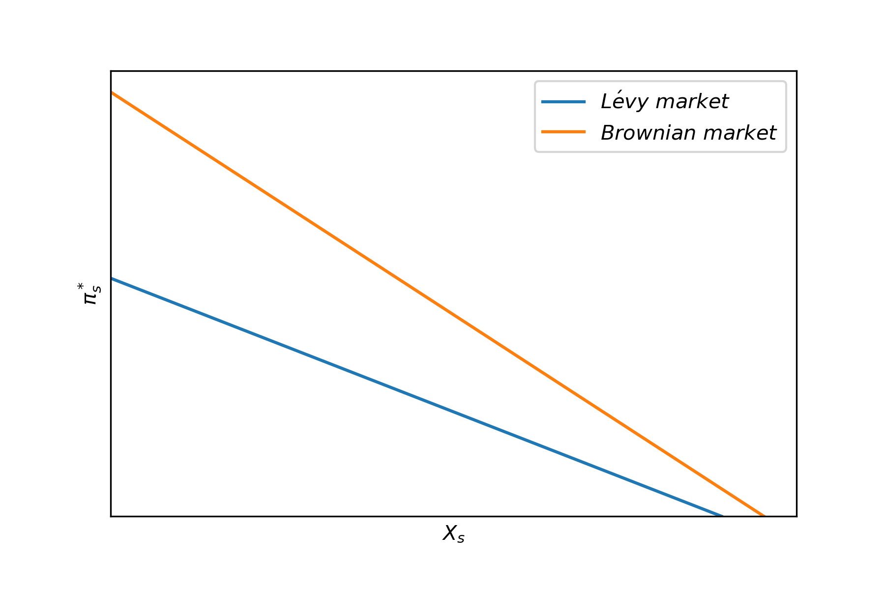
Figure 1: Optimal investment strategies in Lévy and Brownian financial markets

Moreover, we consider the change of the value function (or utility) when the market model changes. Based on the value function, the utility gained by the investor is

$$\mathbb{E}_{x,z,t}\left[X_{T}^{\pi^{*}}\right]-\frac{\theta}{2}Var_{x,z,t}\left(X_{T}^{\pi^{*}}\right)=x-\frac{1}{2\theta}\left[1-e^{\frac{\left(\mu-r\right)^{2}}{\sigma^{2}+\gamma^{2}\nu(\mathbb{R})}(T-t)}\right].$$

Clearly, the existence of jump risk ($\gamma\neq 0$) leads to lower utility for the investor. It is reasonable as the jump part of the risky asset follows a martingale process with zero expectation, which does not provide any extra expected return but more extreme risks. When the variance increases and expected return declines, the investor’s utility decreases.

5.4 Reasonableness of Assumption 1.

After discussing the equivalency of MMV and MV problems, an important question arises: When does Assumption 1 hold? In this subsection, we provide some numerical examples to show the reasonableness of Assumption 1. Similar to Subsection 5.3, for the purpose of tractability we assume that $\mu$, $\sigma$ and $\gamma$ are constants, which means that the stochastic factor $Z$ is absent. Furthermore, we assume that the Lévy process $L$ is a Poisson process $N$ with intensity $\lambda=\nu(\mathbb{R})$.

In this circumstance, the dynamic of risky asset $S$ is:

$$\mathrm{d}S_{t}=S_{t-}\left(\mu\mathrm{d}t+\sigma\mathrm{d}W^{1}_{t}+\gamma\mathrm{d}N_{t}\right).$$

Honore (1998) has studied the problem of the parameter estimation in the above jump diffusion model. They focus on 18 liquid NYSE stocks and give the corresponding parameter estimations. We refer to their estimations to calculate the jump size we concern

$$\zeta\gamma=-\frac{\mu-r}{\sigma^{2}+\gamma^{2}\nu(\mathbb{R})}\gamma.$$

By setting the risk-free rate $r=0.04$, the estimation results are summarized in Table 1.

Table 1: Estimated parameters of different stocks.

	$\alpha$	$\sigma$	$\nu(\mathbb{R})$	$\gamma$	$\zeta\gamma$
AXP	0.2887	0.3118	2.4754	-0.068724	0.156934
CHV	0.2497	0.2463	2.6653	-0.050006	0.155749
DD	0.1779	0.2348	1.2878	-0.056067	0.130648
DOW	0.2044	0.2610	1.6259	-0.061057	0.135311
EK	0.1254	0.2595	0.8759	-0.082956	0.096561
GE	0.2389	0.2219	1.9257	-0.052378	0.191077
GM	0.1460	0.2515	1.8357	-0.053609	0.082924
IBM	0.1214	0.2351	0.7544	-0.075313	0.102945
IP	0.1488	0.2598	0.4890	-0.089990	0.137020
KO	0.2669	0.2392	1.6916	-0.063026	0.223671
MMM	0.1549	0.2135	1.0352	-0.063588	0.146807
MO	0.3067	0.2449	2.2174	-0.057482	0.227783
MOB	0.2388	0.2458	2.0809	-0.058235	0.171578
MRK	0.2656	0.2296	2.6653	-0.042472	0.166567
PG	0.1782	0.2087	0.9792	-0.058989	0.173588
S	0.1540	0.2656	1.2014	-0.064337	0.097124
T	0.1676	0.1977	1.7907	-0.049911	0.146251
XON	0.2135	0.1998	1.9356	-0.047247	0.185291
DAX	0.2243	0.1377	4.6180	-0.030621	0.242300
FTSE100	0.1522	0.1371	0.2963	-0.088260	0.469223
SP100	0.2340	0.1396	2.1543	-0.042089	0.350371
SP500	0.2464	0.1617	4.7382	-0.039211	0.242077
KFX	0.2359	0.1195	6.5222	-0.024397	0.263150

As we can see, $\zeta\gamma$ is positive in all the tested stocks because $\gamma$ is always negative. This implies that Assumption 1 holds almost in the real market. Furthermore, the absolute value $|\zeta\gamma|$ is significantly smaller than $1$, indicating that even when $\gamma>0$ or when $r$ fluctuates within a small range, Assumption 1 will remain valid.

6 Conclusion.

In this paper, we compare the optimal investment problems based on MMV and MV preferences under a jump diffusion and stochastic factor model. In the incomplete Lévy financial market, we prove that the optimal strategies and value functions of MMV and MV investment problems coincide if and only if a crucial assumption holds. Thus, the assumption is a sufficient and necessary condition for the consistency of MMV and MV preferences. When the key assumption violates, the solutions to the two investment problems can be different when there are jump risks in the financial market, which is an important addition to the literature. As Strub and Li (2020) prove that the optimal strategies of MMV and MV problems coincide in any continuous market, we provide an example to show that the discontinuity of asset prices can change such result. Thus, the difference between MMV and MV portfolio selections is due to the discontinuity of the market. Moreover, we provide some empirical evidences to illustrate the reasonableness of the assumption in real financial market. As recent developments in the MMV literature are also concerned with the trading constraints, we think that MMV portfolio selection problems when the market is discontinuous and the strategy is constrained can be further studied in the future.

References

- Bäuerle and Grether [2015] Nicole Bäuerle and Stefanie Grether. Complete markets do not allow free cash flow streams. Mathematical Methods of Operations Research, 81(2):137–146, 2015.
- Bjork and Murgoci [2010] Tomas Bjork and Agatha Murgoci. A general theory of markovian time inconsistent stochastic control problems. 2010. URL http://dx.doi.org/10.2139/ssrn.1694759.
- Černỳ and Kallsen [2007] Aleš Černỳ and Jan Kallsen. On the structure of general mean-variance hedging strategies. The Annals of Probability, 35(4):1479–1531, 2007.
- Chan [1999] Terence Chan. Pricing contingent claims on stocks driven by lévy processes. Annals of Applied Probability, pages 504–528, 1999.
- Du and Strub [2023] Jinye Du and Moris Simon Strub. Monotone and classical mean-variance preferences coincide when asset prices are continuous. Available at SSRN 4359422, 2023.
- Gilboa and Schmeidler [1989] Itzhak Gilboa and David Schmeidler. Maxmin expected utility with non-unique prior. Journal of Mathematical Economics, 18(2):141–153, 1989.
- Honore [1998] Peter Honore. Pitfalls in estimating jump-diffusion models. Available at SSRN 61998, 1998.
- Hu et al. [2023] Ying Hu, Xiaomin Shi, and Zuo Quan Xu. Constrained monotone mean-variance problem with random coefficients. SIAM Journal on Financial Mathematics, 14(3):838–854, 2023.
- Jacod and Shiryaev [2013] Jean Jacod and Albert Shiryaev. Limit theorems for stochastic processes, volume 288. Springer Science & Business Media, 2013.
- Ladyzhenskaya et al. [1968] O.A. Ladyzhenskaya, V.A. Solonnikov, and N.N. Uraltseva. Linear and Quasi-linear Equations of Parabolic Type. Translations of Mathematical Monographs,Volume 23. American Mathematical Society, 1968.
- Li and Guo [2021] Bohan Li and Junyi Guo. Optimal reinsurance and investment strategies for an insurer under monotone mean-variance criterion. RAIRO-Operations Research, 55(4):2469–2489, 2021.
- Li and Ng [2000] Duan Li and Wan-Lung Ng. Optimal dynamic portfolio selection: Multiperiod mean-variance formulation. Mathematical Finance, 10(3):387–406, 2000.
- Li et al. [2002] Xun Li, Xun Yu Zhou, and Andrew EB Lim. Dynamic mean-variance portfolio selection with no-shorting constraints. SIAM Journal on Control and Optimization, 40(5):1540–1555, 2002.
- Lim [2004] Andrew EB Lim. Quadratic hedging and mean-variance portfolio selection with random parameters in an incomplete market. Mathematics of Operations Research, 29(1):132–161, 2004.
- Lim and Zhou [2002] Andrew EB Lim and Xun Yu Zhou. Mean-variance portfolio selection with random parameters in a complete market. Mathematics of Operations Research, 27(1):101–120, 2002.
- Liu [2017] Tai-Ping Liu. Hopf-cole transformation. Bulletin of the Institute of Mathematics Academia Sinica, 12:71–101, 2017.
- Maccheroni et al. [2009] Fabio Maccheroni, Massimo Marinacci, Aldo Rustichini, and Marco Taboga. Portfolio selection with monotone mean-variance preferences. Mathematical Finance, 19(3):487–521, 2009.
- Markowits [1952] Harry M Markowits. Portfolio selection. Journal of Finance, 7(1):71–91, 1952.
- Mataramvura and Øksendal [2008] Sure Mataramvura and Bernt Øksendal. Risk minimizing portfolios and HJBI equations for stochastic differential games. Stochastics, 80(4):317–337, 2008.
- Mémin [2006] Jean Mémin. Décompositions multiplicatives de semimartingales exponentielles et applications. In Séminaire de Probabilités XII: Université de Strasbourg 1976/77, pages 35–46. Springer, 2006.
- Øksendal and Sulem [2007a] Bernt Øksendal and Agnes Sulem. Stochastic Calculus with Jump Diffusions, pages 1–25. Springer Berlin Heidelberg, Berlin, Heidelberg, 2007a. ISBN 978-3-540-69826-5.
- Øksendal and Sulem [2007b] Bernt Øksendal and Agnes Sulem. Stochastic Control of Jump Diffusions, pages 45–63. Springer Berlin Heidelberg, Berlin, Heidelberg, 2007b. ISBN 978-3-540-69826-5.
- Øksendal and Sulem [2014] Bernt Øksendal and Agnès Sulem. Forward–backward stochastic differential games and stochastic control under model uncertainty. Journal of Optimization Theory and Applications, 161(1):22–55, 2014.
- Protter [2005] Philip E. Protter. Stochastic Differential Equations. Springer Berlin Heidelberg, 2005. ISBN 978-3-662-10061-5.
- Shen and Zou [2022] Yang Shen and Bin Zou. Cone-constrained monotone mean-variance portfolio selection under diffusion models. SIAM Journal on Financial Mathematics, 13(4):SC99–SC112, 2022.
- Strub and Li [2020] Moris S Strub and Duan Li. A note on monotone mean–variance preferences for continuous processes. Operations Research Letters, 48(4):397–400, 2020.
- Tankov [2003] Peter Tankov. Financial Modelling with Jump Processes. Chapman and Hall/CRC, 2003. ISBN 978-1-58488-413-4.
- Trybuła and Zawisza [2019] Jakub Trybuła and Dariusz Zawisza. Continuous-time portfolio choice under monotone mean-variance preferences—stochastic factor case. Mathematics of Operations Research, 44(3):966–987, 2019.
- Yong and Zhou [1999] Jiongmin Yong and Xun Yu Zhou. Stochastic Controls: Hamiltonian Systems and HJB Equations, volume 43. Springer Science & Business Media, 1999. ISBN 978-0-387-98723-1.
- Zariphopoulou [2001] Thaleia Zariphopoulou. A solution approach to valuation with unhedgeable risks. Finance and Stochastics, 5(1):61–82, 2001.
- Zawisza [2010] Dariusz Zawisza. Robust portfolio selection under exponential preferences. Applicationes Mathematicae, 37:215–230, 2010.
- Zawisza [2012] Dariusz Zawisza. Target achieving portfolio under model misspecification: quadratic optimization framework. Applicationes Mathematicae, 39:425–443, 2012.
- Zeng et al. [2013] Yan Zeng, Zhongfei Li, and Yongzeng Lai. Time-consistent investment and reinsurance strategies for mean–variance insurers with jumps. Insurance: Mathematics and Economics, 52(3):498–507, 2013.
- Zhou and Li [2000] Xun Yu Zhou and Duan Li. Continuous-time mean-variance portfolio selection: A stochastic LQ framework. Applied Mathematics and Optimization, 42(1):19–33, 2000.