Supplementary Materials for
“SKDBERT: Compressing BERT via Stochastic Knowledge Distillation”

A Multi-teacher Knowledge Distillation

For BERT-style language model compression, we verify the performance of MTBERT (Wu, Wu, and Huang 2021) whose objection function can be expressed as:

$$\mathcal{L}_{\rm MTBERT}=\sum_{i=1}^{N}\frac{{\rm CE}(y_{i}/T,y_{s}/T)}{1+{\rm CE}(y,y_{i})},$$ (1)

where, $N$ indicates the number of teacher models, ${\rm CE}(\cdot,\cdot)$ is the cross-entropy loss, $T$ denotes the temperature, $y$ represents the ground-truth label, $y_{i}$ and $y_{s}$ refer to the outputs of $i$-th teacher model and the student model, respectively. We employ the student model used in TinyBERT (Jiao et al. 2020) which can be downloaded from https://huggingface.co/huawei-noah/TinyB ERT_General_6L_768D. Furthermore, we choose five BERT-style models whose architecture information is shown in Table 1, as the teacher models from the BERT official website.

[t] Teacher Layer Hidden size Head #Params (M) T₀ 8 768 12 81.1 T₁ 10 768 12 95.3 T₂ 12 768 12 110 T₃ 24 1024 16 335 T₄† 24 1024 16 335

Table 1: The architecture information of each teacher model.

• Pre-training with whole word masking.

Furthermore, we fine tune the above teacher models on six downstream tasks of GLUE benchmark, i.e., MRPC, RTE, SST-2, QQP, QNLI and MNLI whose detailed introduction can be found in Section D. Moreover, the experimental settings of teacher models fine-tuning are shown as follows:

• Learning Rate: For T₃ and T₄, {6e-6, 7e-6, 8e-6, 9e-6} on MRPC and RTE tasks, and {2e-5, 3e-5, 4e-5, 5e-5} on other tasks. For other teacher models, {2e-5, 3e-5, 4e-5, 5e-5} on all tasks.

• Batch Size: {32} for teacher model fine-tuning on each task.

• Epoch: 10 for MRPC and RTE, 3 for other tasks.

Other settings are following TinyBERT (Jiao et al. 2020).

Subsequently, we employ the ensemble of the fine-tuned teacher models to compress the student model via (1) . Particularly, we only use the weighted multi-teacher distillation loss without the multi-teacher hidden loss and the task-specific loss as in MT-BERT (Wu, Wu, and Huang 2021).

The experimental settings are given as follows:

• Learning Rate: {1e-5, 2e-5, 3e-5} for all tasks.

• Batch Size: {16, 32, 64}.

• Epoch: 10 for MRPC and RTE, 3 for other tasks.

Similarly, other settings are also following TinyBERT (Jiao et al. 2020).

B SKD for Image Classification

To verify the effectiveness of general SKD on computer vision, we conduct a list of experiments on CIFAR-100 (Krizhevsky, Hinton et al. 2009) image classification dataset. Moreover, we employ ResNet (He et al. 2016) and Wide ResNet (WRN) (Zagoruyko and Komodakis 2016) with various architectures as the candidates of teacher team to distill a student model. Following the experimental settings in CRD (Tian, Krishnan, and Isola 2020), we train the student model and teacher model for 240 epochs, and employ SGD as the optimizer with a batch size of 64, a learning rate of 0.05 which is decayed by a factor of 0.1 when arriving at 150-th, 180-th, 210-th epoch and a weight decay of 5e-4, and show the results in Table 2.

Similar to Tian, Krishnan, and Isola (2020), we show the test accuracy of the last epoch in Table 3 for a fair comparison. The proposed SKD also achieves novel performance on CIFAR-100. Compared to state-of-the-art CRD, our approach achieves the best performance in five out of six groups of distillation experiments.

C Why Does SKD Work?

In this section, taking uniform distribution based SKD as an example, we discuss why does it work.

[tbq] Teacher Student None WRN-40-1 WRN-16-2 ResNet-20 ResNet-32 ResNet-8$\times$4 None - 71.98 73.95 69.06 71.14 72.50 WRN-16-2 73.95 73.85 WRN-22-2 74.26 74.36 75.24 WRN-28-2 74.94 74.28 75.25 WRN-34-2 76.22 74.23 75.16 WRN-40-2 75.61 73.57 75.23 ResNet-26 70.75 69.96 ResNet-32 71.10 70.43 ResNet-38 71.97 70.84 72.83 ResNet-44 72.14 70.99 73.20 ResNet-50 72.49 70.96 72.97 ResNet-56 72.41 71.08 73.21 ResNet-68 73.62 71.03 73.82 ResNet-80 73.67 70.94 73.29 ResNet-92 73.94 71.06 73.44 ResNet-104 73.54 71.11 73.55 ResNet-110 74.31 71.01 73.57 ResNet-14$\times$4 77.07 75.20 ResNet-20$\times$4 77.67 74.43 ResNet-26$\times$4 79.29 73.95 ResNet-32$\times$4 79.42 73.60

Table 2: Accuracy (%) of each student model and each teacher model for the last epoch of vanilla training and average of the best epoch over 5 runs of distillation on the test set of CIFAR-100.

[tbq] Student WRN-16-2 WRN-40-1 ResNet-20 ResNet-20 ResNet-32 ResNet-8$\times$4 Teacher WRN-40-2 WRN-40-2 ResNet-56 ResNet-110 ResNet-110 ResNet-32$\times$4 Acc-S 73.26 71.98 69.06 69.06 71.14 72.50 Acc-T 75.61 75.61 72.34 74.31 74.31 79.42 KD 74.92 73.54 70.66 70.67 73.08 73.33 FitNet 73.58 72.24 69.21 68.99 71.06 73.50 AT 74.08 72.77 70.55 70.22 72.31 73.44 SP 73.83 72.43 69.67 70.04 72.69 72.94 CC 73.56 72.21 69.63 69.48 71.48 72.97 VID 74.11 73.30 70.38 70.16 72.61 73.09 RKD 73.35 72.22 69.61 69.25 71.82 71.90 PKT 74.54 73.45 70.34 70.25 72.61 73.64 AB 72.50 72.38 69.47 69.53 70.98 73.17 FT 73.25 71.59 69.84 70.22 72.37 72.86 FSP 72.91 - 69.95 70.11 71.89 72.62 NST 73.68 72.24 69.60 69.53 71.96 73.30 CRD 75.48 74.14 71.16 71.46 73.48 75.51 TT${\dagger}$ TT₁ TT₂ TT₃ TT₄ TT₅ TT₆ SKD 75.52 74.63 71.16 71.47 73.92 74.79

Table 3: Test accuracy (%) of the proposed SKD and other popular distillation approaches on CIFAR-100. All experimental results are cited from Tian, Krishnan, and Isola (2020). Average of the last epoch over 5 runs.

• Teacher team list:
  TT₁: WRN-22-2, WRN-28-2, WRN-34-2, WRN-40-2
  TT₂: WRN-16-2, WRN-22-2, WRN-28-2, WRN-34-2, WRN-40-2
  TT₃: ResNet-26, ResNet-32, ResNet-38, ResNet-44, ResNet-50, ResNet-56
  TT₄: ResNet-32, ResNet-38, ResNet-44, ResNet-50, ResNet-56, ResNet-68, ResNet-80, ResNet-92, ResNet-104, ResNet-110
  TT₅: ResNet-44, ResNet-50, ResNet-56, ResNet-68, ResNet-80, ResNet-92, ResNet-104, ResNet-110
  TT₆: ResNet-14$\times$4, ResNet-20$\times$4, ResNet-32$\times$4
  

C.1 Preliminaries: Knowledge Distillation

On classification task with $C$ categories, vanilla KD employs the output of final layer, logits $\boldsymbol{z}=[z_{1},z_{2},\dots,z_{C}]^{\rm T}$, to yield soft targets $\boldsymbol{p}=[p_{1},p_{2},\dots,p_{C}]^{\rm T}$ for knowledge transfer as

$$p_{i}=\frac{{\rm exp}(z_{i}/T)}{\sum_{j=1}^{C}{\rm exp}(z_{j}/T)},\quad i=1,2,\dots,C$$

where, $T$ represents the temperature factor which is used to control the importance of $p_{i}$.

The total loss $\mathcal{L}$ with respect to input $\boldsymbol{x}$ and weights of student model $\boldsymbol{W}$, consists of distilled loss $\mathcal{L}_{d}$ and student loss $\mathcal{L}_{s}$ as

$$\mathcal{L}(\boldsymbol{x},\boldsymbol{W})=\alpha\times\mathcal{L}_{d}(p(\boldsymbol{z}_{t},T),p(\boldsymbol{z}_{s},T))+\beta\times\mathcal{L}_{s}(\boldsymbol{y},p(\boldsymbol{z}_{s},T)),$$

where,

$$\mathcal{L}_{d}(p(\boldsymbol{z}_{t},T),p(\boldsymbol{z}_{s},T))=\sum_{i=1}^{C}-p(z_{ti},T){\rm ln}(p(z_{si},T))$$

and

$$\mathcal{L}_{s}(\boldsymbol{y},p(\boldsymbol{z}_{s},T))=\sum_{i=1}^{C}-y_{i}{\rm ln}(p(z_{si},T))$$

treat soft targets $\boldsymbol{p}(\boldsymbol{z}_{t},T)$ and ground truth $\boldsymbol{y}$ as their labels, respectively. Moreover, $\boldsymbol{z}_{t}$ and $\boldsymbol{z}_{s}$ represent the logits of teacher and student models, respectively. Particularly, an ensemble of multiple teacher models is used to provide

C.2 The Convergence of SKD

In order to optimize $\boldsymbol{W}$, we should evaluate the cross-entropy gradient of total loss with regard to $z_{si}$, $\frac{\partial\mathcal{L}(\boldsymbol{x},\boldsymbol{W})}{\partial z_{si}}$ as

$$\alpha\times\frac{\partial\mathcal{L}_{d}(p(\boldsymbol{z}_{t},T),p(\boldsymbol{z}_{s},T))}{\partial z_{si}}+\beta\times\frac{\partial\mathcal{L}_{s}(\boldsymbol{y},p(\boldsymbol{z}_{s},T))}{\partial z_{si}}.$$ (2)

Here, the second term of the right side of (2) of SKD is identical with vanilla KD, so that we only discuss the first term.

The cross-entropy gradient of distilled loss with regard to $z_{si}$ can be computed as

$$\begin{split}&\frac{\partial\mathcal{L}_{d}(p(\boldsymbol{z}_{t},T),p(\boldsymbol{z}_{s},T))}{\partial z_{si}}\\ &=\frac{\partial\sum_{k=1}^{C}-p(z_{tk},T){\rm ln}(p(z_{sk},T))}{\partial z_{si}}\\ &=\frac{\partial\sum_{k=1}^{C}-p(z_{tk},T){\rm ln}(p(z_{sk},T))}{\partial{\rm ln}(p(z_{sj},T))}\times\frac{\partial{\rm ln}(p(z_{sj},T))}{\partial z_{si}}\\ &=-\sum_{k=1}^{C}p(z_{tk},T)\frac{1}{p(z_{sk},T)}\times\frac{\partial{\rm ln}(p(z_{sj},T))}{\partial z_{si}}.\end{split}$$ (3)

For $\frac{\partial{\rm ln}(p(z_{sj},T))}{\partial z_{si}}$, there are two situations (i.e., $i=j$ and $i\neq j$) as

$$\left\{\begin{split}&\frac{1}{T}{\rm ln}(p(z_{si},T))\times(1-{\rm ln}(p(z_{si},T))),\quad if\,\,\,i=j\\ &-\frac{1}{T}{\rm ln}(p(z_{si},T)\times{\rm ln}(p(z_{sj},T)).\quad\quad\,\,\,others\\ \end{split}\right.$$ (4)

Subsequently, we replace $\frac{\partial{\rm ln}(p(z_{sj},T))}{\partial z_{si}}$ in (3) with (4), and it can be rewritten as

$$\begin{split}&\frac{\partial\mathcal{L}_{d}(p(\boldsymbol{z}_{t},T),p(\boldsymbol{z}_{s},T))}{\partial z_{si}}\\ &=-\sum_{k=1}^{C}\frac{p(z_{tk},T)}{{\rm ln}(p(z_{sk},T))}\times\frac{\partial{\rm ln}(p(z_{sj},T))}{\partial z_{si}}\\ &=-\frac{p(z_{ti},T)}{{\rm ln}(p(z_{si},T))}\times\frac{{\rm ln}(p(z_{si},T))\times(1-{\rm ln}(p(z_{si},T)))}{T}\\ &+\sum_{j\neq i}\left(\frac{p(z_{tj},T)}{{\rm ln}(p(z_{sj},T))}\times\frac{{\rm ln}(p(z_{si},T))\times{\rm ln}(p(z_{sj},T))}{T}\right)\\ &=-\frac{p(z_{ti},T)-p(z_{ti},T){\rm ln}(p(z_{si},T))}{T}\\ &+\frac{\sum_{j\neq i}p(z_{tj},T){\rm ln}(p(z_{si},T))}{T}\\ &=\frac{\sum_{j=1}^{C}p(z_{tj},T){\rm ln}(p(z_{si},T))-p(z_{ti},T)}{T}\\ &=\frac{{\rm ln}(p(z_{si},T))-p(z_{ti},T)}{T}.\end{split}$$

On the one hand, in vanilla multi-teacher KD framework with an ensemble of $N$ teacher models, $z_{ti}$ is the average of ensemble as

$$z_{ti}=\frac{1}{N}\sum_{n=1}^{N}z_{ti}^{(n)},$$

so that its soft target can be computed as

$$p_{\rm Avg}(z_{ti},T)=\frac{{\rm exp}(\frac{\frac{1}{N}\sum_{n=1}^{N}z_{ti}^{(n)}}{T})}{\sum_{j=1}^{C}{\rm exp}(\frac{\frac{1}{N}\sum_{n=1}^{N}z_{tj}^{(n)}}{T})}.$$

On the other hand, SKD randomly employs a single teacher from $N$ teacher models to obtain the soft target at $n$-th iteration as

$$p_{\rm SKD}^{(n)}(z_{ti},T)=\frac{{\rm exp}(\frac{z_{ti}^{(n)}}{T})}{\sum_{j=1}^{C}{\rm exp}(\frac{z_{tj}^{(n)}}{T})},$$

where, the sampled probability of $\boldsymbol{z}_{t}^{(n)}$ subjects to uniform distribution ${\rm U}(1,N)$.

We assume that the number of iterations is $L$. In the total training process of multi-teacher KD, the amount of gradient update on $z_{i}$ dubbed $G_{\rm Avg}^{(i)}$ can be represented as

$$\begin{split}&\sum_{l=1}^{L}\frac{{\rm ln}(p(z_{si}^{(l)},T))-\frac{{\rm exp}(\frac{\frac{1}{N}\sum_{n=1}^{N}z_{ti}^{(n)}}{T})}{\sum_{j=1}^{C}{\rm exp}(\frac{\frac{1}{N}\sum_{n=1}^{N}z_{tj}^{(n)}}{T})}}{T}\\ &=\frac{1}{T}\sum_{l=1}^{L}{\rm ln}(p(z_{si}^{(l)},T))-\frac{L}{T}\times\underbrace{\frac{{\rm exp}(\frac{\frac{1}{N}\sum_{n=1}^{N}z_{ti}^{(n)}}{T})}{\sum_{j=1}^{C}{\rm exp}(\frac{\frac{1}{N}\sum_{n=1}^{N}z_{tj}^{(n)}}{T})}}_{a_{i}}.\end{split}$$ (5)

Beyond that, the amount of gradient update of SKD on $z_{i}$ dubbed $G_{\rm SKD}^{(i)}$ can be obtained by

$$\begin{split}G_{\rm SKD}^{(i)}&=\sum_{l=1}^{L}\frac{{\rm ln}(p(z_{si}^{(l)},T))-\frac{{\rm exp}(\frac{z_{ti}^{(n)}}{T})}{\sum_{j=1}^{C}{\rm exp}(\frac{z_{tj}^{(n)}}{T})}}{T}\\ &=\frac{1}{T}\sum_{l=1}^{L}{\rm ln}(p(z_{si}^{(l)},T))-\frac{L}{T}\times\underbrace{\frac{{\rm exp}(\frac{z_{ti}^{(n)}}{T})}{\sum_{j=1}^{C}{\rm exp}(\frac{z_{tj}^{(n)}}{T})}}_{b_{i}}\end{split}$$ (6)

Obviously, the main difference between $G_{\rm Avg}^{(i)}$ and $G_{\rm SKD}^{(i)}$ is the terms of $a_{i}$ in (5) and $b_{i}$ in (6). We denote $\frac{\sum_{n=1}^{N}z_{ti}^{(n)}}{N}$ as $\overline{z}_{ti}$, and rewrite term $a_{i}$ in (5) as

$$\begin{split}a_{i}=\frac{{\rm exp}(\frac{\overline{z}_{ti}}{T})}{\sum_{j=1}^{C}{\rm exp}(\frac{\overline{z}_{tj}}{T})}.\end{split}$$ (7)

According to (7) and the term $b_{i}$ in (6), we can find that their relationship is similar to the relationship between Batch Gradient Descent (BGD) and Stochastic Gradient Descent (SGD). Moreover, BGD employs total data to obtain the gradient in each iteration, but SGD uses single one. Based on stochastic approximation (e.g. ROBBINS-MONRO’s theory (Robbins and Monro 1951)) and convex optimization, the convergence of SGD has been proven (Turinici 2021).

D Details of GLUE Benchmark

GLUE consists of 9 NLP tasks: Microsoft Research Paraphrase Corpus (MRPC) (Dolan and Brockett 2005), Recognizing Textual Entailment (RTE) (Bentivogli et al. 2009), Corpus of Linguistic Acceptability (CoLA) (Warstadt, Singh, and Bowman 2019), Semantic Textual Similarity Benchmark (STS-B) (Cer et al. 2017), Stanford Sentiment Treebank (SST-2) (Socher et al. 2013), Quora Question Pairs (QQP) (Chen et al. 2018), Question NLI (QNLI) (Rajpurkar et al. 2016), Multi-Genre NLI (MNLI) (Williams, Nangia, and Bowman 2017), and Winograd NLI (WNLI) (Levesque, Davis, and Morgenstern 2012).

MRPC

belongs to a sentence similarity task where system aims to identify the paraphrase/semantic equivalence relationship between two sentences.

RTE

belongs to a natural language inference task where system aims to recognize the entailment relationship of given two text fragments.

CoLA

belongs to a single-sentence task where system aims to predict the grammatical correctness of an English sentence.

STS-B

belongs to a sentence similarity task where system aims to evaluate the similarity of two pieces of texts by a score from 1 to 5.

SST-2

belongs to a single-sentence task where system aims to predict the sentiment of movie reviews.

QQP

belongs to a sentence similarity task where system aims to identify the semantical equivalence of two questions from the website Quora.

QNLI

belongs to a natural language inference task where system aims to recognize that for a given pair <question, context>, the answer to the question whether contains in the context.

MNLI

belongs to a natural language inference task where system aims to predict the possible relationships (i.e., entailment, contradiction and neutral) of hypothesis with regard to premise for a given pair <premise, hypothesis>,.

WNLI

belongs to a natural language inference task where system aims to determine the referent of a sentence’s pronoun from a list of choices.

E Evaluation Metrics and Hyper-parameters

E.1 Evaluation Metrics

In order to choose the best model, we use appropriate metrics on GLUE-dev as shown in Table 4.

[tbq] Task Metric Description STS-B $\frac{pear+spear}{2}$ $pear$ and $spear$ are Pearson and Spearman correlation coefficients, respectively. MNLI $acc$-$m$ $acc$-$m$ means accuracy on matched section. MRPC, QQP $\frac{acc+f1}{2}$ $acc$ represents accuracy, $f1$ indicates F1 scores. SST-2, QNLI, RTE $acc$ None

Table 4: Evaluation metrics on GLUE-dev.

E.2 Fine-tuning Hyper-parameters

In this paper, we need to perform teacher model fine-tuning, student model fine-tuning and student model distillation. For the above three cases, the used hyper-parameters are shown in Table 5.

[tbq] Hyper-parameter Value Learning rate For large teacher models, [6e-6, 7e-6, 8e-6, 9e-6] on MRPC and RTE tasks, [2e-5, 3e-5, 4e-5, 5e-5] on other tasks. For other teacher models and student models, [2e-5, 3e-5, 4e- 5, 5e-5] and [1e-5, 2e-5, 3e-5] on all tasks, respectively. Adam $\epsilon$ 1e-6 Adam $\beta_{1}$ 0.9 Adam $\beta_{2}$ 0.999 Learning rate decay linear Warmup fraction 0.1 Attention dropout 0.1 Dropout 0.1 Weight decay 1e-4 Batch size 32 for fine-tuning, [16, 32] for distillation Fine-tuning epochs For KD, WKD and TAKD, 10 on MRPC, RTE and STS-B tasks, 3 on other tasks. For SKD, 15 on MRPC, RTE and STS-B tasks, 5 on other tasks

Table 5: Hyper-parameters for fine-tuning and distillation.

[t] Model Name Layer Hidden Size Head #Params (M) Student SKDBERT₄ 4 312 12 14.5 SKDBERT₆ 6 768 12 67.0 Teacher T₀₁ 8 128 2 5.6 T₀₂ 10 128 2 6.0 T₀₃ 12 128 2 6.4 T₀₄ 8 256 4 14.3 T₀₅ 10 256 4 15.9 T₀₆ 12 256 4 17.5 T₀₇ 8 512 8 41.4 T₀₈ 10 512 8 47.7 T₀₉ 12 512 8 54.0 T₁₀ 8 768 12 81.1 T₁₁ 10 768 12 95.3 T₁₂ 12 768 12 110 T₁₃ 24 1024 16 335 T₁₄† 24 1024 16 335

Table 6: The architecture of each student and teacher model.

• Pre-training with whole word masking.

F Student Model and Teacher Team Details

The architecture information of each student model and teacher model is shown in Table 6. On the one hand, we direct treating the pre-trained model of TinyBERT₄ and TinyBERT₆ as the student models of SKDBERT. On the other hand, we choose 14 BERT models with various capabilities as the candidates for teacher team. Moreover, each pre-trained teacher model can be downloaded from official implementation of BERT. Furthermore, the results of the student model and the teacher model on GLUE-dev are shown in Table 7 which can be used to obtain the teacher-rank sampling distribution.

[tbq] Model MRPC RTE STS-B SST-2 QQP QNLI MNLI-m Avg SKDBERT₄ 83.83 63.90 84.86 87.84 84.64 83.83 76.18 80.73 SKDBERT₆ 89.44 71.84 88.52 91.63 86.44 90.70 82.55 85.87 T₀₁ 81.83 66.06 85.15 86.24 83.95 83.80 72.95 80.00 T₀₂ 84.75 66.06 84.99 85.67 84.18 84.00 73.75 80.49 T₀₃ 84.59 65.70 85.73 86.47 85.02 84.40 75.16 81.01 T₀₄ 85.18 64.62 86.77 89.33 86.36 86.80 78.16 82.46 T₀₅ 87.84 66.06 87.45 89.33 87.25 87.26 78.75 83.42 T₀₆ 85.96 66.06 87.00 89.68 87.21 87.42 79.54 83.27 T₀₇ 87.91 70.04 88.46 91.28 88.69 89.27 80.84 85.21 T₀₈ 88.17 65.70 88.75 91.28 88.62 89.25 81.41 84.74 T₀₉ 88.85 66.43 88.74 92.09 89.01 90.33 81.90 85.34 T₁₀ 89.36 68.95 89.03 93.00 89.27 90.79 83.05 86.21 T₁₁ 90.10 71.12 89.59 92.78 89.71 91.20 84.00 86.93 T₁₂ 89.98 68.59 90.20 92.66 89.66 91.85 84.40 86.76 T₁₃ 90.60 62.74 90.13 94.50 90.26 92.70 86.88 86.83 T₁₄ 90.15 79.06 91.21 94.72 90.40 93.89 87.06 89.50

Table 7: The fine-tuning performance of each student and teacher models on GLUE-dev.

G Distillation Performance of SKDBERT with Various Teacher Models

In order to determine the student-rank sampling distribution for SKD, we employ each teacher model to distill SKDBERT₄ and SKDBERT₆ on GLUE-dev, and show the results in Table 8.

[tbq] Student Teacher MRPC RTE STS-B SST-2 QQP QNLI MNLI-m SKDBERT₄ None 83.83 63.90 84.86 87.84 84.64 83.83 76.18 SKDBERT₄ T₀₁ 81.73 ($\downarrow$) 62.82 ($\downarrow$) 84.90 ($\uparrow$) 86.93 ($\downarrow$) 83.54 ($\downarrow$) 83.60 ($\downarrow$) 73.39 ($\downarrow$) T₀₂ 83.55 ($\downarrow$) 64.62 ($\uparrow$) 84.63 ($\downarrow$) 87.39 ($\downarrow$) 84.01 ($\downarrow$) 83.82 ($\downarrow$) 73.81 ($\downarrow$) T₀₃ 83.88 ($\uparrow$) 65.34 ($\uparrow$) 84.91 ($\uparrow$) 87.73 ($\downarrow$) 84.75 ($\uparrow$) 83.75 ($\downarrow$) 74.90 ($\downarrow$) T₀₄ 82.73 ($\downarrow$) 63.90 ($\uparrow$) 84.74 ($\downarrow$) 88.07 ($\uparrow$) 85.26 ($\uparrow$) 85.23 ($\uparrow$) 76.58 ($\uparrow$) T₀₅ 85.25 ($\uparrow$) 67.15 ($\uparrow$) 84.66 ($\downarrow$) 87.84 ($\uparrow$) 85.48 ($\uparrow$) 85.34 ($\uparrow$) 76.94 ($\uparrow$) T₀₆ 86.25 ($\uparrow$) 66.06 ($\uparrow$) 85.05 ($\uparrow$) 87.50 ($\downarrow$) 85.40 ($\uparrow$) 85.94 ($\uparrow$) 77.30 ($\uparrow$) T₀₇ 85.31 ($\uparrow$) 64.98 ($\uparrow$) 85.11 ($\uparrow$) 88.53 ($\uparrow$) 85.32 ($\uparrow$) 84.77 ($\uparrow$) 77.53 ($\uparrow$) T₀₈ 84.27 ($\uparrow$) 65.34 ($\uparrow$) 85.17 ($\uparrow$) 88.19 ($\uparrow$) 85.59 ($\uparrow$) 85.52 ($\uparrow$) 77.84 ($\uparrow$) T₀₉ 84.01 ($\uparrow$) 66.79 ($\uparrow$) 84.67 ($\downarrow$) 88.30 ($\uparrow$) 85.39 ($\uparrow$) 85.63 ($\uparrow$) 77.15 ($\uparrow$) T₁₀ 84.87 ($\uparrow$) 65.70 ($\uparrow$) 84.55 ($\downarrow$) 87.96 ($\uparrow$) 85.30 ($\uparrow$) 85.37 ($\uparrow$) 77.82 ($\uparrow$) T₁₁ 83.96 ($\uparrow$) 65.34 ($\uparrow$) 84.96 ($\uparrow$) 88.65 ($\uparrow$) 85.44 ($\uparrow$) 85.04 ($\uparrow$) 77.36 ($\uparrow$) T₁₂ 85.24 ($\uparrow$) 65.70 ($\uparrow$) 85.03 ($\uparrow$) 89.22 ($\uparrow$) 85.32 ($\uparrow$) 85.58 ($\uparrow$) 77.40 ($\uparrow$) T₁₃ 85.35 ($\uparrow$) 66.43 ($\uparrow$) 84.87 ($\uparrow$) 88.30 ($\uparrow$) 85.13 ($\uparrow$) 84.88 ($\uparrow$) 77.08 ($\uparrow$) T₁₄ 84.42 ($\uparrow$) 66.43 ($\uparrow$) 84.87 ($\uparrow$) 87.73 ($\downarrow$) 85.29 ($\uparrow$) 84.51 ($\uparrow$) 76.73 ($\uparrow$) SKDBERT₆ None 89.44 71.84 88.52 91.63 86.44 90.70 82.55 SKDBERT₆ T₀₁ 84.61 ($\downarrow$) 67.87 ($\downarrow$) 88.78 ($\uparrow$) 88.76 ($\downarrow$) 84.63 ($\downarrow$) 86.33 ($\downarrow$) 74.87 ($\downarrow$) T₀₂ 87.94 ($\downarrow$) 67.15 ($\downarrow$) 88.73 ($\uparrow$) 89.68 ($\downarrow$) 85.07 ($\downarrow$) 86.20 ($\downarrow$) 75.31 ($\downarrow$) T₀₃ 87.08 ($\downarrow$) 70.76 ($\downarrow$) 88.95 ($\uparrow$) 90.48 ($\downarrow$) 86.08 ($\downarrow$) 86.53 ($\downarrow$) 76.21 ($\downarrow$) T₀₄ 89.72 ($\uparrow$) 68.95 ($\downarrow$) 89.16 ($\uparrow$) 92.43 ($\uparrow$) 87.09 ($\uparrow$) 89.57 ($\downarrow$) 79.67 ($\downarrow$) T₀₅ 89.73 ($\uparrow$) 71.12 ($\downarrow$) 88.81 ($\uparrow$) 91.40 ($\downarrow$) 87.77 ($\uparrow$) 89.82 ($\downarrow$) 79.84 ($\downarrow$) T₀₆ 88.36 ($\downarrow$) 69.31 ($\downarrow$) 88.91 ($\uparrow$) 92.43 ($\uparrow$) 87.60 ($\uparrow$) 90.24 ($\downarrow$) 80.42 ($\downarrow$) T₀₇ 89.46 ($\uparrow$) 73.65 ($\uparrow$) 88.81 ($\uparrow$) 92.78 ($\uparrow$) 88.64 ($\uparrow$) 90.99 ($\uparrow$) 81.93 ($\downarrow$) T₀₈ 89.56 ($\uparrow$) 71.48 ($\downarrow$) 89.07 ($\uparrow$) 92.32 ($\uparrow$) 88.76 ($\uparrow$) 90.90 ($\uparrow$) 82.27 ($\downarrow$) T₀₉ 89.85 ($\uparrow$) 72.20 ($\uparrow$) 89.02 ($\uparrow$) 92.20 ($\uparrow$) 88.92 ($\uparrow$) 91.51 ($\uparrow$) 82.70 ($\uparrow$) T₁₀ 89.59 ($\uparrow$) 73.29 ($\uparrow$) 89.06 ($\uparrow$) 91.97 ($\uparrow$) 88.88 ($\uparrow$) 91.07 ($\uparrow$) 82.86 ($\uparrow$) T₁₁ 89.73 ($\uparrow$) 71.84 ($\uparrow$) 88.95 ($\uparrow$) 92.32 ($\uparrow$) 88.98 ($\uparrow$) 91.27 ($\uparrow$) 83.17 ($\uparrow$) T₁₂ 89.13 ($\downarrow$) 71.48 ($\downarrow$) 89.02 ($\uparrow$) 93.12 ($\uparrow$) 88.90 ($\uparrow$) 91.40 ($\uparrow$) 82.83 ($\uparrow$) T₁₃ 90.01 ($\uparrow$) 72.92 ($\uparrow$) 88.86 ($\uparrow$) 92.09 ($\uparrow$) 88.89 ($\uparrow$) 91.16 ($\uparrow$) 83.42 ($\uparrow$) T₁₄ 89.50 ($\uparrow$) 72.56 ($\uparrow$) 88.86 ($\uparrow$) 92.43 ($\uparrow$) 89.03 ($\uparrow$) 91.32 ($\uparrow$) 83.46 ($\uparrow$)

Table 8: The distillation performance of SKDBERT with various teacher models on GLUE-dev. $\uparrow$ indicates that the distillation performance is better than SKDBERT without KD. $\downarrow$ indicates that the distillation performance is worse than SKDBERT without KD.

H The Used Sampling Distributions for SKDBERT with Various Teacher Teams on The GLUE Benchmark

We implement extensive ablation experiments for SKDBERT using various teacher teams: {T₀₄-T₀₆, T₀₇-T₀₉, T₁₀-T₁₂, T₁₂-T₁₄} for SKDBERT₄ and {T₀₄-T₀₆, T₀₇-T₀₉, T₁₀-T₁₂, T₀₄-T₀₉, T₀₄-T₁₂, T₀₁-T₁₄, T₀₄-T₁₄, T₀₇-T₁₄, T₀₉-T₁₄, T₁₂-T₁₄, T₁₃-T₁₄} for SKDBERT₆. We show the used distributions for the above teacher teams on various tasks in Figure 1 to 15. Particular, 0 indicates that the teacher models are not employed for stochastic knowledge distillation.

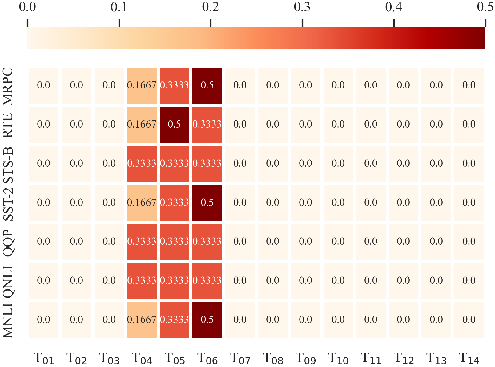
Figure 1: The sampling distribution of SKDBERT₄ with the teacher team of T₀₄ to T₀₆ on the GLUE benchmark.

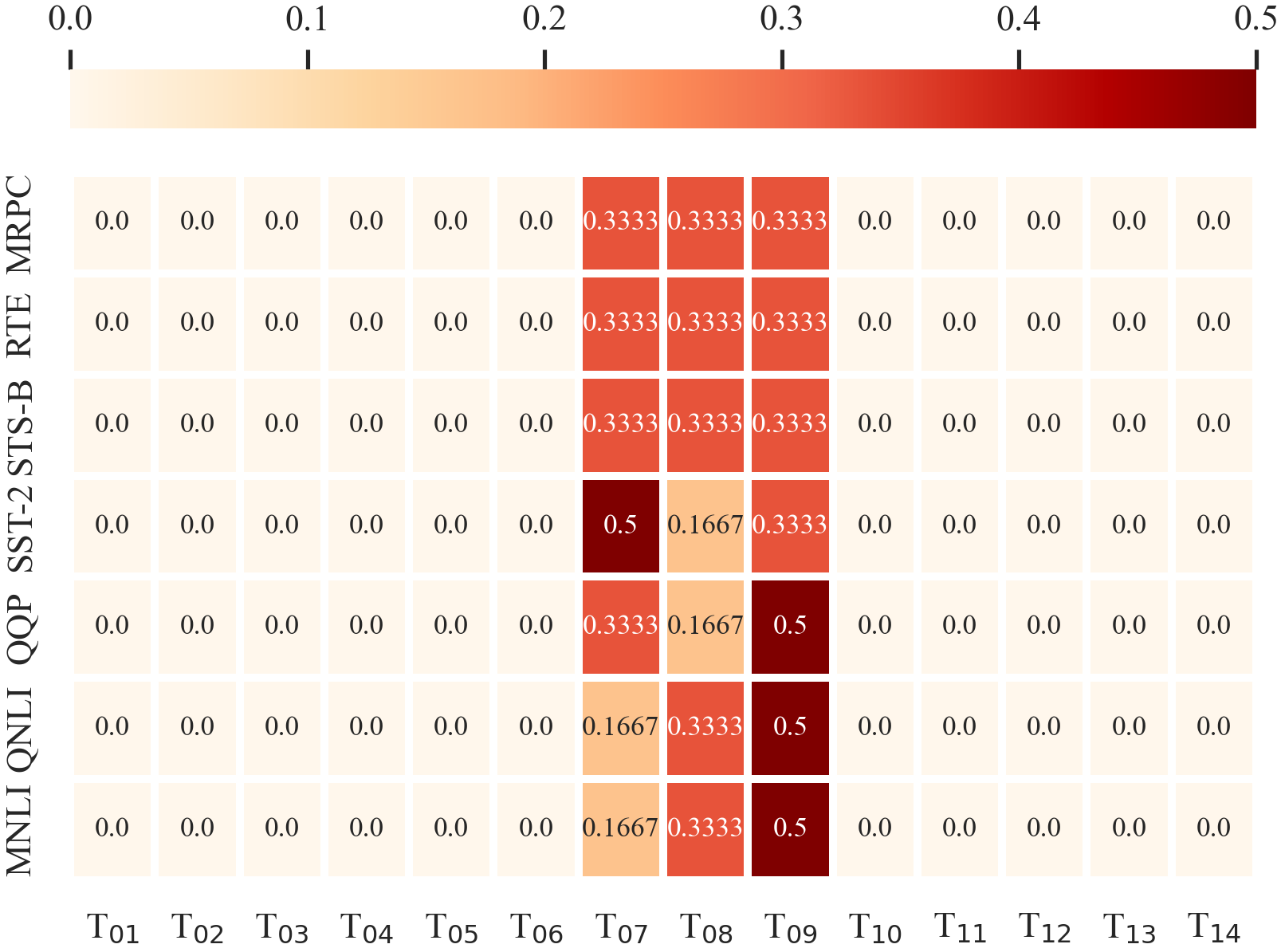
Figure 2: The sampling distribution of SKDBERT₄ with the teacher team of T₀₇ to T₀₉ on the GLUE benchmark.

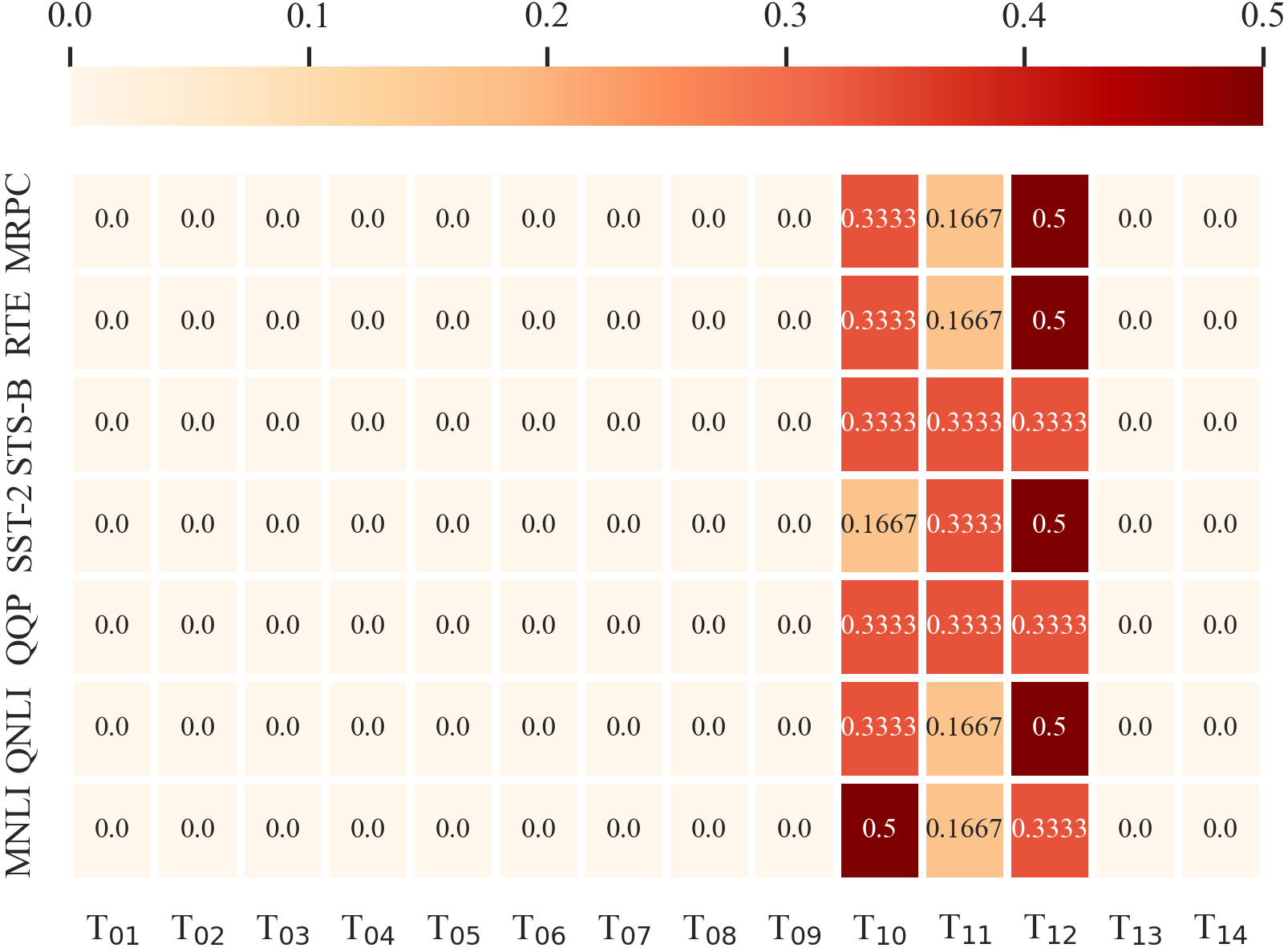
Figure 3: The sampling distribution of SKDBERT₄ with the teacher team of T₁₀ to T₁₂ on the GLUE benchmark.

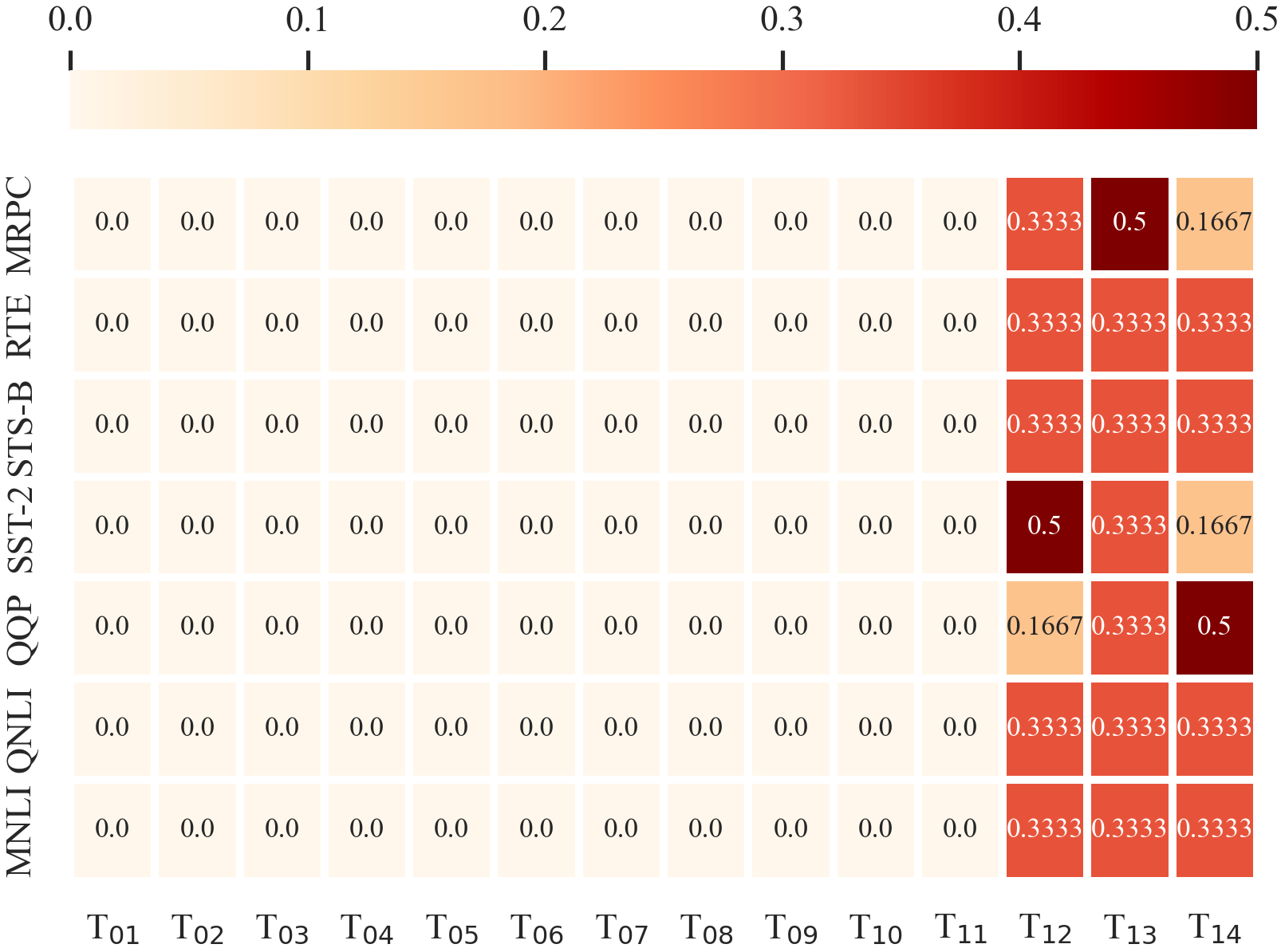
Figure 4: The sampling distribution of SKDBERT₄ with the teacher team of T₁₂ to T₁₄ on the GLUE benchmark.

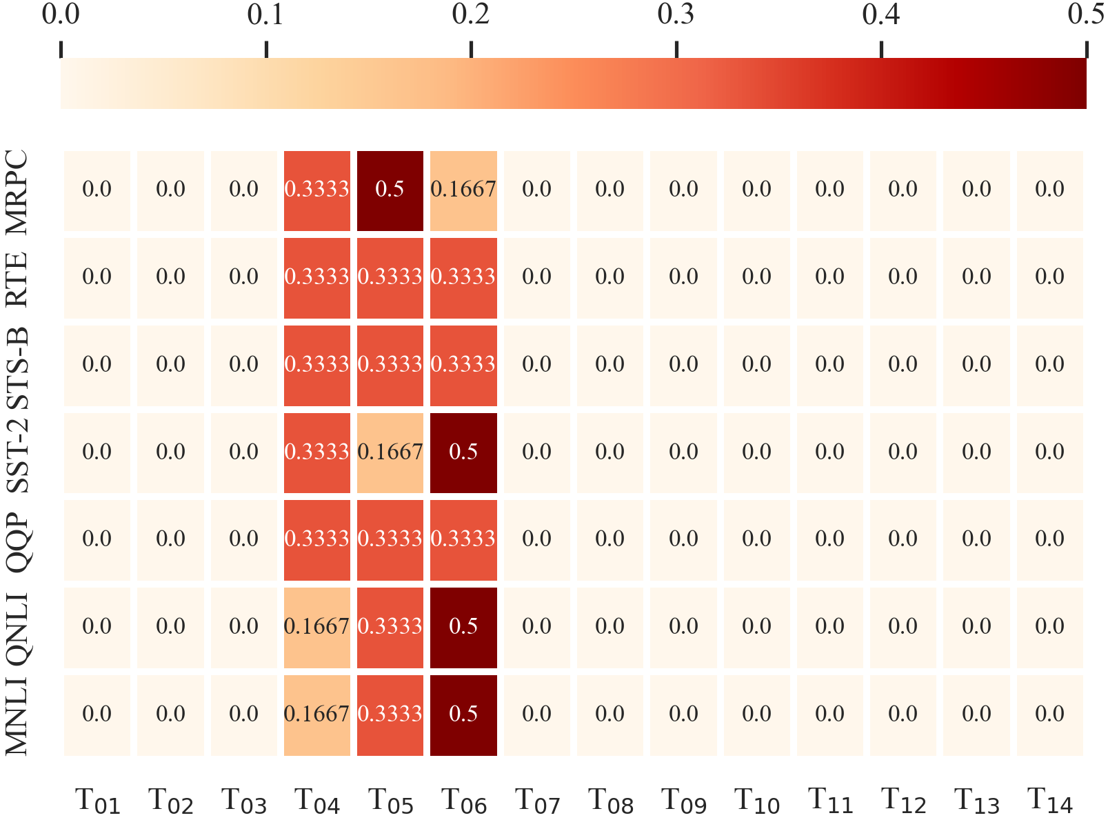
Figure 5: The sampling distribution of SKDBERT₆ with the teacher team of T₀₄ to T₀₆ on the GLUE benchmark.

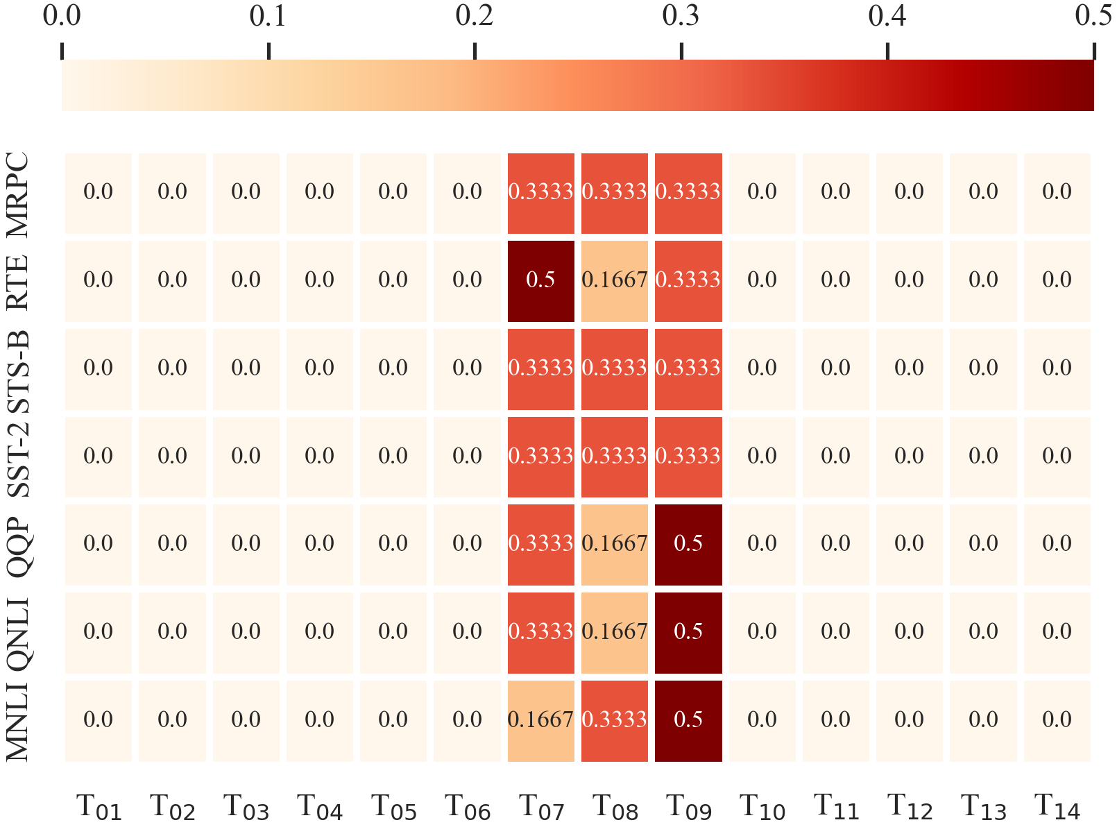
Figure 6: The sampling distribution of SKDBERT₆ with the teacher team of T₀₇ to T₀₉ on the GLUE benchmark.

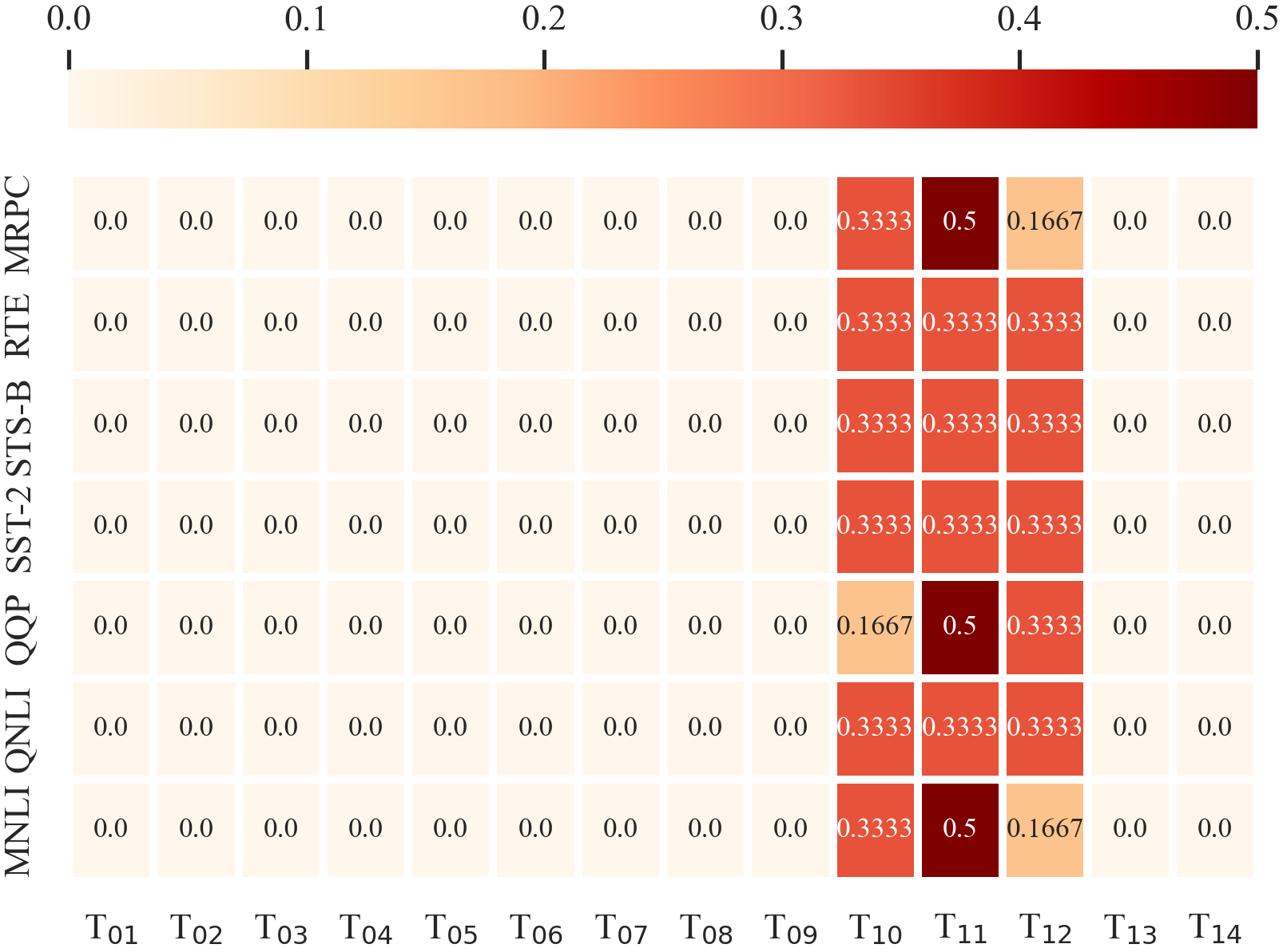
Figure 7: The sampling distribution of SKDBERT₆ with the teacher team of T₁₀ to T₁₂ on the GLUE benchmark.

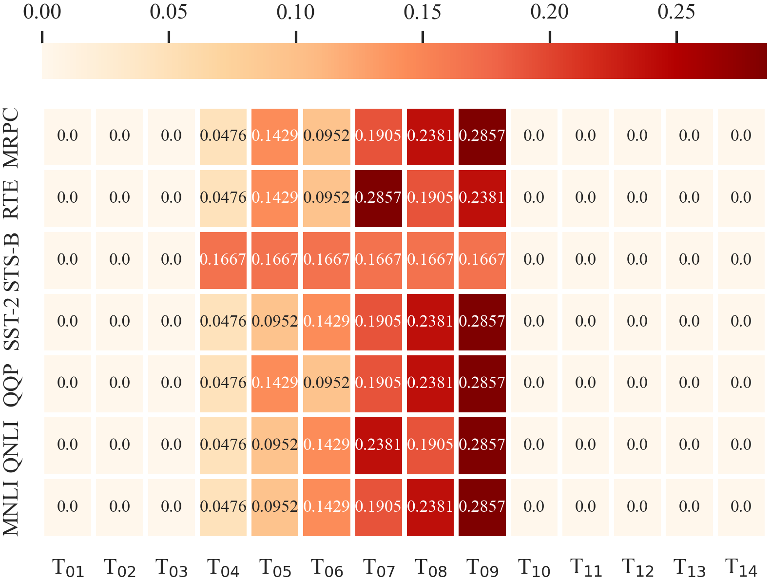
Figure 8: The sampling distribution of SKDBERT₆ with the teacher team of T₀₄ to T₀₉ on the GLUE benchmark.

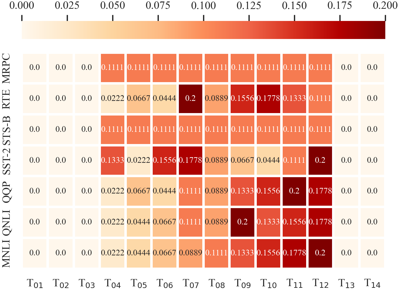
Figure 9: The sampling distribution of SKDBERT₆ with the teacher team of T₀₄ to T₁₂ on the GLUE benchmark.

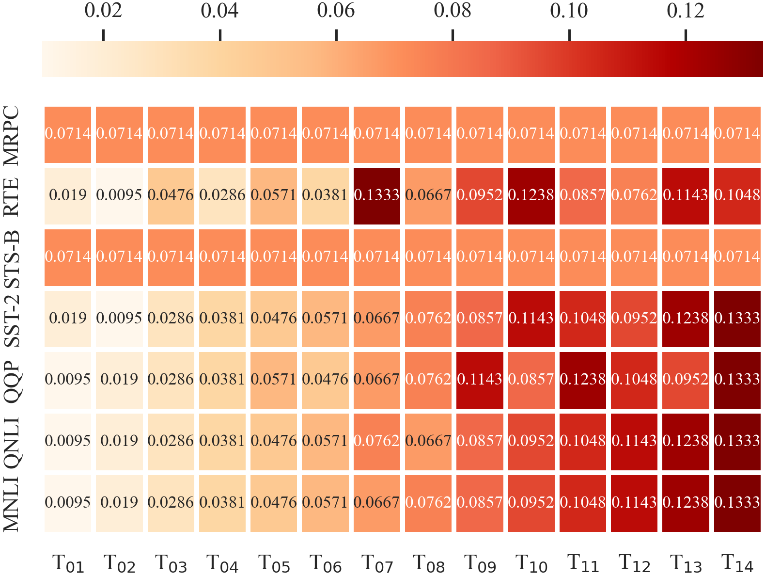
Figure 10: The sampling distribution of SKDBERT₆ with the teacher team of T₀₁ to T₁₄ on the GLUE benchmark.

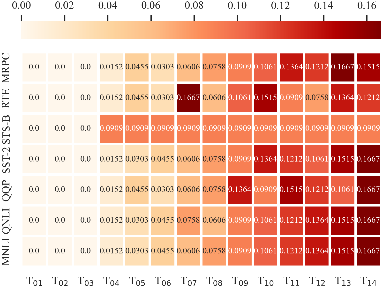
Figure 11: The sampling distribution of SKDBERT₆ with the teacher team of T₀₄ to T₁₄ on the GLUE benchmark.

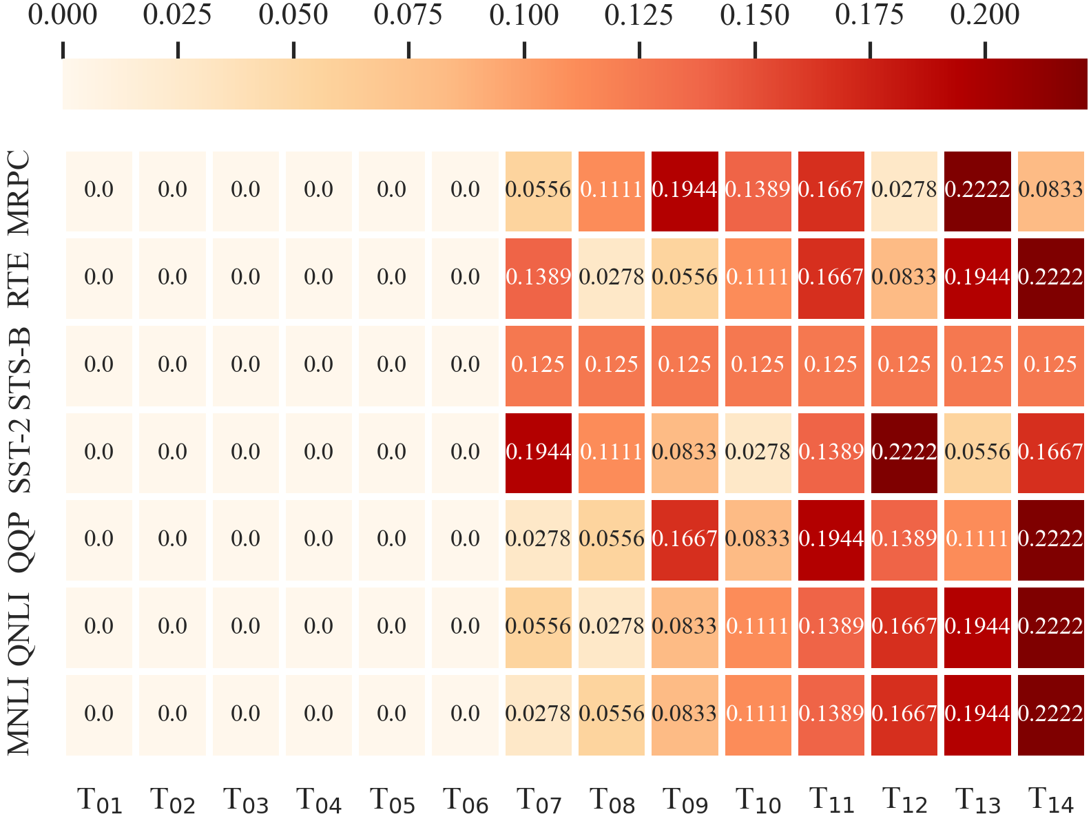
Figure 12: The sampling distribution of SKDBERT₆ with the teacher team of T₀₇ to T₁₄ on the GLUE benchmark.

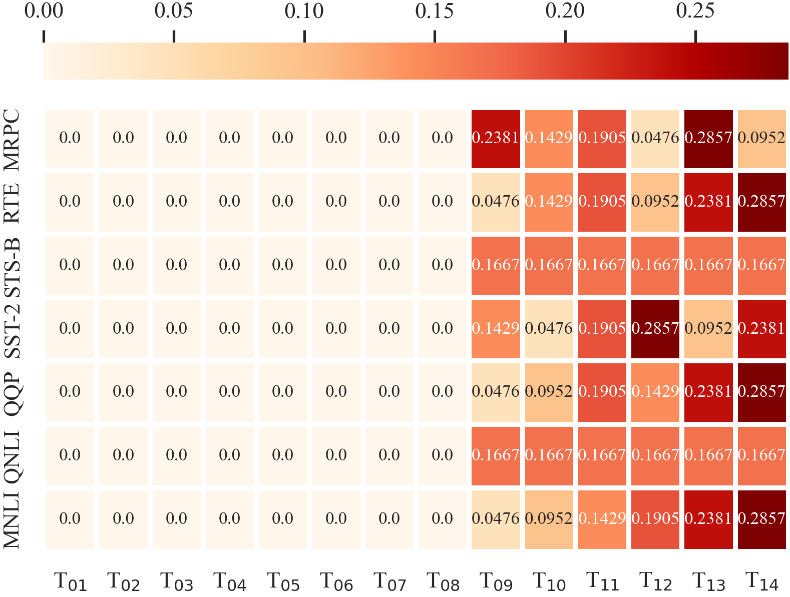
Figure 13: The sampling distribution of SKDBERT₆ with the teacher team of T₀₉ to T₁₄ on the GLUE benchmark.

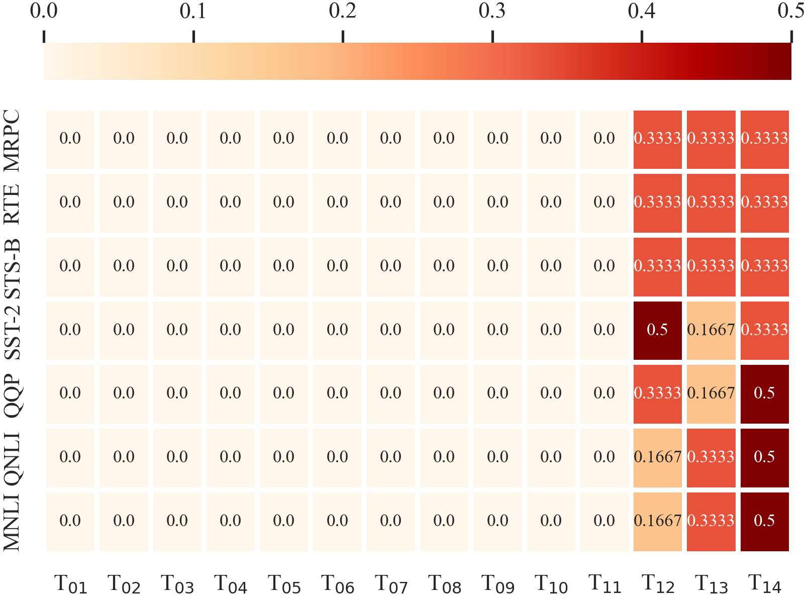
Figure 14: The sampling distribution of SKDBERT₆ with the teacher team of T₁₂ to T₁₄ on the GLUE benchmark.

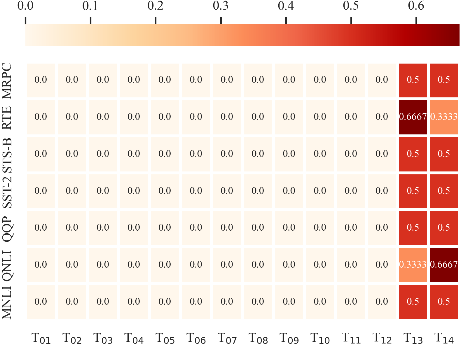
Figure 15: The sampling distribution of SKDBERT₆ with the teacher team of T₁₃ to T₁₄ on the GLUE benchmark.

References

- Bentivogli et al. (2009) Bentivogli, L.; Clark, P.; Dagan, I.; and Giampiccolo, D. 2009. The Fifth PASCAL Recognizing Textual Entailment Challenge. In TAC.
- Cer et al. (2017) Cer, D.; Diab, M.; Agirre, E.; Lopez-Gazpio, I.; and Specia, L. 2017. Semeval-2017 task 1: Semantic textual similarity-multilingual and cross-lingual focused evaluation. In Proceedings of the 11th Inter- national Workshop on Semantic Evaluation.
- Chen et al. (2018) Chen, Z.; Zhang, H.; Zhang, X.; and Zhao, L. 2018. Quora question pairs. University of Waterloo, 1–7.
- Dolan and Brockett (2005) Dolan, B.; and Brockett, C. 2005. Automatically constructing a corpus of sentential paraphrases. In Third International Workshop on Paraphrasing, IWP.
- He et al. (2016) He, K.; Zhang, X.; Ren, S.; and Sun, J. 2016. Deep residual learning for image recognition. In Proceedings of the IEEE conference on Computer Vision and Pattern Recognition, CVPR, 770–778.
- Jiao et al. (2020) Jiao, X.; Yin, Y.; Shang, L.; Jiang, X.; Chen, X.; Li, L.; Wang, F.; and Liu, Q. 2020. TinyBERT: Distilling BERT for Natural Language Understanding. In Proceedings of the 2020 Conference on Empirical Methods in Natural Language Processing, EMNLP, 4163–4174.
- Krizhevsky, Hinton et al. (2009) Krizhevsky, A.; Hinton, G.; et al. 2009. Learning multiple layers of features from tiny images.
- Levesque, Davis, and Morgenstern (2012) Levesque, H.; Davis, E.; and Morgenstern, L. 2012. The winograd schema challenge. In Thirteenth international conference on the principles of knowledge representation and reasoning.
- Rajpurkar et al. (2016) Rajpurkar, P.; Zhang, J.; Lopyrev, K.; and Liang, P. 2016. SQuAD: 100, 000+ Questions for Machine Comprehension of Text. In Proceedings of the 2016 Conference on Empirical Methods in Natural Language Processing, EMNLP, 2383–2392.
- Robbins and Monro (1951) Robbins, H.; and Monro, S. 1951. A stochastic approximation method. The annals of mathematical statistics, 400–407.
- Socher et al. (2013) Socher, R.; Perelygin, A.; Wu, J.; Chuang, J.; Manning, C. D.; Ng, A. Y.; and Potts, C. 2013. Recursive deep models for semantic compositionality over a sentiment treebank. In Proceedings of the 2013 Conference on Empirical Methods in Natural Language Processing, EMNLP, 1631–1642.
- Tian, Krishnan, and Isola (2020) Tian, Y.; Krishnan, D.; and Isola, P. 2020. Contrastive representation distillation. In 8th International Conference on Learning Representations, ICLR.
- Turinici (2021) Turinici, G. 2021. The convergence of the Stochastic Gradient Descent (SGD): A self-contained proof. arXiv preprint arXiv:2103.14350.
- Warstadt, Singh, and Bowman (2019) Warstadt, A.; Singh, A.; and Bowman, S. R. 2019. Neural network acceptability judgments. Transactions of the Association for Computational Linguistics, 7: 625–641.
- Williams, Nangia, and Bowman (2017) Williams, A.; Nangia, N.; and Bowman, S. R. 2017. A broad-coverage challenge corpus for sentence understanding through inference. In Proceedings of the 2017 Conference of the North American Chapter of the Association for Computational Linguistics, NAACL.
- Wu, Wu, and Huang (2021) Wu, C.; Wu, F.; and Huang, Y. 2021. One teacher is enough? pre-trained language model distillation from multiple teachers. In Findings of the Association for Computational Linguistics: ACL/IJCNLP, 4408–4413.
- Zagoruyko and Komodakis (2016) Zagoruyko, S.; and Komodakis, N. 2016. Wide residual networks. In Proceedings of the British Machine Vision Conference 2016, BMVC.