c-TPE: Tree-Structured Parzen Estimator with Inequality Constraints
for Expensive Hyperparameter Optimization

Abstract

Hyperparameter optimization (HPO) is crucial for strong performance of deep learning algorithms and real-world applications often impose some constraints, such as memory usage, or latency on top of the performance requirement. In this work, we propose constrained TPE (c-TPE), an extension of the widely-used versatile Bayesian optimization method, tree-structured Parzen estimator (TPE), to handle these constraints. Our proposed extension goes beyond a simple combination of an existing acquisition function and the original TPE, and instead includes modifications that address issues that cause poor performance. We thoroughly analyze these modifications both empirically and theoretically, providing insights into how they effectively overcome these challenges. In the experiments, we demonstrate that c-TPE exhibits the best average rank performance among existing methods with statistical significance on $81$ expensive HPO with inequality constraints. Due to the lack of baselines, we only discuss the applicability of our method to hard-constrained optimization in Appendix D.

1 Introduction

While deep learning (DL) has achieved various breakthrough successes, its performance highly depends on the proper settings of its hyperparameters Chen et al. (2018); Melis et al. (2018). Furthermore, practical applications often impose several constraints on memory usage or latency of inference, making it necessary to apply constrained hyperparameter optimization (HPO).

Recent developments in constrained HPO have led to the emergence of new acquisition functions (AFs) Gardner et al. (2014); Lobato et al. (2015); Eriksson and Poloczek (2021) in Bayesian optimization (BO) with Gaussian process (GP), which judge the promise of a configuration based on the surrogate model. While GP-based methods offer theoretical advantages, recent open source softwares (OSS) for HPO, such as Optuna Akiba et al. (2019), Hyperopt Bergstra et al. (2013), and Ray Liaw et al. (2018), instead employ the tree-structured Parzen estimator (TPE) Bergstra et al. (2011, 2013); Watanabe (2023), a variant of BO using the density ratio of kernel density estimators for good and bad observations, as the main algorithm, and Optuna played a pivotal role for HPO of DL models in winning Kaggle competitions Alina et al. (2019); Addison et al. (2022). Despite its versatility for expensive HPO problems, the existing AFs are not directly applicable to TPE and no study has been conducted on TPE’s extension to constrained optimization.

In this paper, we propose c-TPE, a constrained optimization method that generalizes TPE. We first show that it is possible to integrate the original TPE into the existing AF proposed by Gelbart et al. Gelbart et al. (2014), which uses the product of AFs for the objective and each constraint, and thus TPE can be generalized with constrained settings. Then, a naïve extension, which calculates AF by the product of density ratios for the objective and each constraint with the same split algorithm, could be simply obtained; however, the naïve extension suffers from performance degradation under some circumstances. To circumvent these pitfalls, we propose (1) the split algorithm that includes a certain number of feasible solutions, and (2) AF by the product of relative density ratios, and analyze their effects empirically and theoretically.

In the experiments, we demonstrate (1) the strong performance of c-TPE with statistical significance on expensive HPO problems and (2) robustness to changes in the constraint level. Notice that we briefly discuss the applicability of our method to hard-constrained optimization in Appendix D, and we discuss the limitations of our work in Appendix E caused by our choices of search spaces that are limited to tabular benchmarks to enable the stability analysis of the performance variations depending on constraint levels.

In summary, the main contributions of this paper are to:

1. prove that TPE can be extended to constrained settings using the AF proposed by Gelbart et al. Gelbart et al. (2014),

2. present two pitfalls in the naïve extension and describe how our modifications mitigate those issues,

3. provide the stability analysis of the performance variations depending on constraint levels, and

4. demonstrate that the proposed method outperforms existing methods with statistical significance on average on $9$ tabular benchmarks with $27$ different settings.

The implementation and the experiment scripts are available at https://github.com/nabenabe0928/constrained-tpe/.

2 Background

2.1 Bayesian Optimization (BO)

Suppose we would like to minimize a validation loss metric $f(\bm{x})=\mathcal{L}(\bm{x},\mathcal{A},\mathcal{D}_{\rm train},\mathcal{D}_{\rm val})$ of a supervised learning algorithm $\mathcal{A}$ given training and validation datasets $\mathcal{D}_{\rm train},\mathcal{D}_{\rm val}$, then the HPO problem is defined as follows:

$$\bm{x}_{\mathrm{opt}}\in\mathop{\mathrm{argmin}}_{\bm{x}\in\mathcal{X}}f(\bm{x}).$$ (1)

Note that $\bm{x}\in\mathcal{X}$ is a hyperparameter configuration, $\mathcal{X}=\mathcal{X}_{1}\times\dots\times\mathcal{X}_{D}$ is the search space of the hyperparameter configurations, and $\mathcal{X}_{d}\subseteq\mathbb{R}~{}(\text{for }d=1,\dots,D)$ is the domain of the $d$-th hyperparameter. In Bayesian optimization (BO) Brochu et al. (2010); Shahriari et al. (2016); Garnett (2022), we assume that $f(\bm{x})$ is expensive and consider the optimization in a surrogate space given a set of observations $\mathcal{D}\coloneqq\{(\bm{x}_{n},f_{n})\}_{n=1}^{N}$. In each iteration of BO, we build a predictive model $p(f|\bm{x},\mathcal{D})$ and optimize an AF to yield the next configuration. A common choice for AF is the following expected improvement (EI) Jones et al. (1998):

$$\mathrm{EI}_{f^{\star}}[\bm{x}|\mathcal{D}]=\int_{-\infty}^{f^{\star}}(f^{\star}-f)p(f|\bm{x},\mathcal{D})df.$$ (2)

Another common choice is the following probability of improvement (PI) Kushner (1964):

$$\mathbb{P}[f\leq f^{\star}|\bm{x},\mathcal{D}]=\int_{-\infty}^{f^{\star}}p(f|\bm{x},\mathcal{D})df.$$ (3)

2.2 Tree-Structured Parzen Estimator (TPE)

TPE Bergstra et al. (2011, 2013) is a variant of BO methods and it uses EI. See Watanabe Watanabe (2023) to better understand the algorithm components. To transform Eq. (2), we assume the following:

$$p(\bm{x}|f,\mathcal{D})=\left\{\begin{array}[]{ll}p(\bm{x}|\mathcal{D}^{(l)})&(f\leq f^{\gamma})\\ p(\bm{x}|\mathcal{D}^{(g)})&(f>f^{\gamma})\end{array}\right.$$ (6)

where $\mathcal{D}^{(l)},\mathcal{D}^{(g)}$ are the observations with $f_{n}\leq f^{\gamma}$ and $f_{n}>f^{\gamma}$, respectively. Note that $f^{\gamma}$ is the top-$\gamma$ quantile objective value in $\mathcal{D}$ at each iteration and $p(\bm{x}|\mathcal{D}^{(l)}),p(\bm{x}|\mathcal{D}^{(g)})$ are built by the kernel density estimator Bergstra et al. (2011, 2013); Falkner et al. (2018). Combining Eqs. (2), (6) and Bayes’ theorem, the AF of TPE is computed as Bergstra et al. (2011):

$$\mathrm{EI}_{f^{\star}}[\bm{x}|\mathcal{D}] \stackrel{{\scriptstyle\mathrm{rank}}}{{\simeq}}r(\bm{x}|\mathcal{D})\coloneqq p(\bm{x}|\mathcal{D}^{(l)})/p(\bm{x}|\mathcal{D}^{(g)})$$ (7)

where $\phi(\bm{x})\stackrel{{\scriptstyle\mathrm{rank}}}{{\simeq}}\psi(\bm{x})$ implies the order isomorphic and $\forall\bm{x},\bm{x}^{\prime}\in\mathcal{X},\phi(\bm{x})\leq\phi(\bm{x}^{\prime})\Leftrightarrow\psi(\bm{x})\leq\psi(\bm{x}^{\prime})$ holds and we use $f^{\star}=f^{\gamma}$ at each iteration. In each iteration, TPE samples configurations from $p(\bm{x}|\mathcal{D}^{(l)})$ and takes the configuration that achieves the maximum $r(\bm{x}|\mathcal{D})$.

2.3 Bayesian Optimization with Unknown Constraints

We consider unknown constraints $c_{i}(\bm{x})=\mathcal{C}_{i}(\bm{x},\mathcal{A},\mathcal{D}_{\rm train},\mathcal{D}_{\rm val})$, e.g. memory usage of the algorithm $\mathcal{A}$ given the configuration $\bm{x}$. Then the optimization is formulated as follows:

$$\begin{gathered}\bm{x}_{\mathrm{opt}}\in\mathop{\mathrm{argmin}}_{\bm{x}\in\mathcal{X}}f(\bm{x})\\ \text{subject to }\forall i\in\{1,\dots,C\},c_{i}(\bm{x})\leq c_{i}^{\star}\end{gathered}$$ (8)

where $c_{i}^{\star}\in\mathbb{R}$ is a threshold for the $i$-th constraint. Note that we reverse the sign of inequality if constraints must be larger than a given threshold. To extend BO to constrained optimization, the following expected constraint improvement (ECI) has been proposed Gelbart et al. (2014):

$$\mathrm{ECI}_{f^{\star}}[\bm{x}|\bm{c}^{\star},\mathcal{D}]=\mathrm{EI}_{f^{\star}}[\bm{x}|\mathcal{D}]\mathbb{P}(c_{1}\leq c_{1}^{\star},\dots,c_{C}\leq c_{C}^{\star}|\bm{x},\mathcal{D}).$$ (9)

where $\bm{c}^{\star}=[c_{1}^{\star},\dots,c_{C}^{\star}]\in\mathbb{R}^{C}$ and $\mathcal{D}=\{(\bm{x}_{n},f_{n},\bm{c}_{n})\}_{n=1}^{N}$ is a set of observations, and $\bm{c}_{n}=[c_{1,n},\dots,c_{C,n}]\in\mathbb{R}^{C}$ is the $n$-th observation of each constraint. However, the following simplified factorized form is the common choice:

$$\mathrm{ECI}_{f^{\star}}[\bm{x}|\bm{c}^{\star},\mathcal{D}]=\mathrm{EI}_{f^{\star}}[\bm{x}|\mathcal{D}]\prod_{i=1}^{C}\mathbb{P}(c_{i}\leq c_{i}^{\star}|\bm{x},\mathcal{D}),$$ (10)

Since there are few methods available for hard-constrained optimization, we only discuss the applicability of our method to hard-constrained optimization in Appendix D.

3 Constrained TPE (c-TPE)

In this section, we first prove that TPE can be extended to constrained settings via the simple product of AFs. Then we describe an extension naïvely inspired by the original TPE and discuss two pitfalls hindering efficient search. Finally, we present modifications for those pitfalls and analyze the effects on toy problems.

Note that throughout this paper, we use the terms $\gamma$-quantile value $f^{\gamma}$ as the top-$\gamma$ quantile function value, ${\gamma_{c^{\star}}}$ as the quantile of $c^{\star}$, and $\Gamma$-feasible domain as the feasible domain in the search space $\mathcal{X}$ that covers $100\times\Gamma\%$ of $\mathcal{X}$. For the formal definitions, see Appendix A.1. Furthermore, we consider two assumptions mentioned in Appendix A.2 and those assumptions allow the whole discussion to be extended to search spaces with categorical parameters.

3.1 Naïve Acquisition Function

Suppose we would like to solve constrained optimization problems formalized in Eq. (8) with ECI. To realize ECI in TPE, we first show the following proposition.

Proposition 1

$\mathrm{EI}_{f^{\star}}[\bm{x}\mid\mathcal{D}]\propto\mathbb{P}(f\leq f^{\star}\mid\bm{x},\mathcal{D})$ holds under the $\mathrm{TPE}$ formulation.

The proof is provided in Appendix A.3. Since PI and EI are equivalent under the TPE formulation, we obtain the following by combining Proposition 1 and Eq. (10):

$$\mathrm{ECI}_{f^{\star}}[\bm{x}|\bm{c}^{\star},\mathcal{D}] \propto\underbrace{\mathbb{P}(f\leq f^{\star}|\bm{x},\mathcal{D})}_{\stackrel{{\scriptstyle\mathrm{rank}}}{{\simeq}}r_{0}(\bm{x}|\mathcal{D})}\prod_{i=1}^{C}\underbrace{\mathbb{P}(c_{i}\leq c_{i}^{\star}|\bm{x},\mathcal{D})}_{\stackrel{{\scriptstyle\mathrm{rank}}}{{\simeq}}r_{i}(\bm{x}|\mathcal{D})}.$$ (11)

Note that we provide the definition of $r_{i}(\bm{x}|\mathcal{D})$ for $i\in\{0,1,\dots,C\}$ in the next section.

3.2 Two Pitfalls in Naïve Extension

Algorithm 1 c-TPE algorithm (With modifications)

1:$N_{\mathrm{init}}$ (The number of initial configurations), $N_{s}$ (The number of candidates to consider in the optimization of the AF)

2:$\mathcal{D}\leftarrow\emptyset$

3:for $n=1,\dots,N_{\mathrm{init}}$ do

4:     Randomly pick $\bm{x}$

5:     $\mathcal{D}\leftarrow\mathcal{D}\cup\{(\bm{x},f(\bm{x}),c_{1}(\bm{x}),\dots,c_{C}(\bm{x}))\}$

6:while Budget is left do

7:     $\mathcal{S}=\emptyset$

8:     for $i=0,\dots,C$ do

9:         Split $\mathcal{D}$ into $\mathcal{D}^{(l)}_{i}$ and $\mathcal{D}^{(g)}_{i}$, $\hat{\gamma}_{i}\leftarrow|\mathcal{D}^{(l)}_{i}|/|\mathcal{D}|$

10:         Build $p(\cdot|\mathcal{D}^{(l)}_{i}),p(\cdot|\mathcal{D}^{(g)}_{i})$

11:         $\{\bm{x}_{j}\}_{j=1}^{N_{s}}\sim p(\cdot|\mathcal{D}^{(l)}_{i}),\mathcal{S}\leftarrow\mathcal{S}\cup\{\bm{x}_{j}\}_{j=1}^{N_{s}}$      

12:     $\triangleright$ See Appendix D for the hard-constrained version

13:     Pick $\bm{x}_{\mathrm{opt}}\in\mathop{\mathrm{argmax}}_{\bm{x}\in\mathcal{S}}\prod_{i=0}^{C}r^{\mathrm{rel}}_{i}(\bm{x}|\mathcal{D})$

14:     $\mathcal{D}\leftarrow\mathcal{D}\cup\{(\bm{x}_{\mathrm{opt}},f(\bm{x}_{\mathrm{opt}}),c_{1}(\bm{x}_{\mathrm{opt}}),\dots,c_{C}(\bm{x}_{\mathrm{opt}}))\}$

3.2.1 Naïve Extension and Modifications

From the discussion above, we could naïvely extend the original TPE to constrained settings using the split in Eq. (6) and the AF in Eq. (7). More specifically, the naïve extension computes the AF as follows:

1. Pick the $\lceil\gamma|\mathcal{D}|\rceil$-th best objective value $f^{\star}$ in $\mathcal{D}$,

2. Split $\mathcal{D}$ into $\mathcal{D}^{(l)}_{0}$ and $\mathcal{D}^{(g)}_{0}$ at $f^{\star}$, and $\mathcal{D}$ into $\mathcal{D}^{(l)}_{i}$ and $\mathcal{D}^{(g)}_{i}$ at $c_{i}^{\star}$ for $i\in\{1,\dots,C\}$,

3. Build kernel density estimators $p(\bm{x}|\mathcal{D}^{(l)}_{i})$, $p(\bm{x}|\mathcal{D}^{(g)}_{i})$ for $i\in\{0,\dots,C\}$, and

4. Take the product of density ratios $\prod_{i=0}^{C}r_{i}(\bm{x}|\mathcal{D})\coloneqq\prod_{i=0}^{C}p(\bm{x}|\mathcal{D}^{(l)}_{i})/p(\bm{x}|\mathcal{D}^{(g)}_{i})$ as the AF.

Note that as $c_{i}^{\star}$ is a user-defined threshold, $c_{i}^{\star}$ is fixed during the optimization. Although this implementation could be naturally inspired by the original TPE, Operations 1 and 4 could incur performance degradation under (1) small overlaps in top domains for the objective and feasible domains, or (2) vanished constraints.

For this reason, we change Operations 1 and 4 as follows:

• Pick the $\lceil\gamma|\mathcal{D}|\rceil$-th best feasible objective value $f^{\star}$ in $\mathcal{D}$ (Line 9), and

• Take the product of relative density ratios $\prod_{i=0}^{C}r^{\mathrm{rel}}_{i}(\bm{x}|\mathcal{D})\coloneqq\prod_{i=0}^{C}(\hat{\gamma}_{i}+(1-\hat{\gamma}_{i})r_{i}(\bm{x}|\mathcal{D})^{-1})^{-1}$ as the AF (Line 13).

Note that we color-coded the modifications in Algorithm 1 and we define $\hat{\gamma}_{i}\coloneqq|\mathcal{D}^{(l)}_{i}|/|\mathcal{D}|$. Intuitively, when all configurations satisfy the $i$-th constraint, i.e. $|\mathcal{D}^{(l)}_{i}|=|\mathcal{D}|\Rightarrow\hat{\gamma}_{i}=1$, we trivially yield $r^{\mathrm{rel}}_{i}=1$; therefore, the $i$-th constraint will be ignored and it is equivalent to $\forall\bm{x}\in\mathcal{X},\mathbb{P}[c_{i}\leq c_{|}^{\star}\bm{x},\mathcal{D}]=1$. Additionally, the following corollary guarantees the mathematical validity of our algorithm:

Corollary 1

$\mathrm{ECI}_{f^{\star}}[\bm{x}|\bm{c}^{\star},\mathcal{D}]\propto\prod_{i=0}^{C}r^{\mathrm{rel}}_{i}(\bm{x}|\mathcal{D})$ under the $\mathrm{TPE}$ formulation.

We provide the proof in Appendix A.4.

The split algorithm in the original TPE by Bergstra et al. Bergstra et al. (2013) first sorts the observations $\mathcal{D}$ by $f$ and takes the first $\lceil\sqrt{N}/4\rceil$ observations as $\mathcal{D}^{(l)}_{0}$ and the rest as $\mathcal{D}^{(g)}_{0}$. On the other hand, our method includes all the observations until the $\lceil\sqrt{N}/4\rceil$-th feasible observations into $\mathcal{D}^{(l)}_{0}$ and the rest into $\mathcal{D}^{(g)}_{0}$, and this split algorithm matches the original algorithm when $\Gamma=1$. For the split of constraints, we first check the upper bound of $\{c_{i,n}\}_{n=1}^{N}$ that satisfies a given threshold $c_{i}^{\star}$ and let this value be $c_{i}^{\prime}$. Note that $c_{i,n}$ is the $i$-th constraint value in the $n$-th observation. If such values do not exist, we take the best value $\min\{c_{i,n}\}_{n=1}^{N}$ so that the optimization of this constraint will be strengthened (see Theorem 1). Then we split $\mathcal{D}$ into $\mathcal{D}^{(l)}_{i}$ and $\mathcal{D}^{(g)}_{i}$ so that $\mathcal{D}^{(l)}_{i}$ includes only observations that satisfy $c_{i,n}\leq c_{i}^{\prime}$ and vice versa. We describe more details in Appendix B and the applicability to hard-constrained optimization in Appendix D. We start the discussion of why these modifications mitigate the issues in the next section.

3.2.2 Issue I: Vanished Constraints

We refer to constraints that are satisfied in almost all configurations as vanished constraints. In other words, if the $i$-th constraint $c_{i}$ is a vanished constraint, its quantile is $\hat{\gamma}_{i}\coloneqq\hat{\gamma}_{c_{i}^{\star}}\simeq 1$. In this case, $r_{i}(\bm{x}|\mathcal{D})$ should be a constant value as $\mathbb{P}(c_{i}\leq c_{i}^{\star}|\bm{x},\mathcal{D})=1$ holds for almost all configurations $\bm{x}$. As discussed in Section 3.2.1, the relative density ratio $r^{\mathrm{rel}}_{i}(\bm{x}|\mathcal{D})$ resolves this issue and it can be written more formally as follows:

Corollary 2

Assuming the feasible domain quantile $\Gamma=1$, then $\prod_{i=0}^{C}r^{\mathrm{rel}}_{i}(\bm{x}|\mathcal{D})\stackrel{{\scriptstyle\mathrm{rank}}}{{\simeq}}r_{0}(\bm{x}|\mathcal{D})$ holds.

Recall that we previously defined $r_{0}(\bm{x}|\mathcal{D})\coloneqq p(\bm{x}|\mathcal{D}^{(l)}_{0})/p(\bm{x}|\mathcal{D}^{(g)}_{0})$ for $\mathcal{D}^{(l)}_{0},\mathcal{D}^{(g)}_{0}$ obtained by splitting $\mathcal{D}$ at $f^{\star}$. The proof is provided in Appendix A.6. Corollary 2 indicates that the AF of c-TPE is equivalent to that of the original TPE when $\Gamma=1$ and it means that our formulation achieves $\mathbb{P}(c_{i}\leq c_{i}^{\star}|\bm{x},\mathcal{D})=1$ if $\hat{\gamma}_{i}=1$. Corollary 2 is a special case of the following theorem:

Theorem 1

Given a pair of constraint thresholds $c_{i}^{\star},c_{j}^{\star}$ and the corresponding quantiles $\hat{\gamma}_{i},\hat{\gamma}_{j}(\hat{\gamma}_{i}\leq\hat{\gamma}_{j})$, if $r_{i}+\frac{\hat{\gamma}_{i}}{1-\hat{\gamma}_{i}}r_{i}^{2}\leq r_{j}+\frac{\hat{\gamma}_{j}}{1-\hat{\gamma}_{j}}r_{j}^{2}$ holds, then

$$\frac{\partial\prod_{k=0}^{C}r^{\mathrm{rel}}_{k}(\bm{x}|\mathcal{D})}{\partial r_{i}}\geq\frac{\partial\prod_{k=0}^{C}r^{\mathrm{rel}}_{k}(\bm{x}|\mathcal{D})}{\partial r_{j}}\geq 0$$ (12)

holds where the first equality holds if $\hat{\gamma}_{i}=\hat{\gamma}_{j}$ and $r_{i}=r_{j}$ and the second one holds iff $\hat{\gamma}_{j}=1$.

The proof is provided in Appendix A.5. Roughly speaking, Theorem 1 implies that our modified AF puts more priority on the variations of the density ratios with lower quantiles, i.e. $r_{i}$ in the statement above, when $r_{i}=r_{j}$.

Figure 1: Heat maps of the AF in the naïve extension (Left column) and our c-TPE (Right column) with a tight (Top row, $c_{1}=4$) or loose (Bottom row, $c_{1}=16$) constraint. For fair comparisons, we use a fixed set of $200$ randomly sampled configurations to compute the AF for all settings. In principle, red regions have higher AF values and the next configuration is likely to be picked from here.

We empirically and intuitively present the effect of Theorem 1 in Figure 1. We used the objective function $f(x,y)=(x+2)^{2}+(y+2)^{2}$ and the constraint $c_{1}(x,y)=(x-1)^{2}+(y-1)^{2}\leq c_{1}^{\star}\in\{4,16\}$ and visualize the heat maps of the AF using exactly the same observations for each figure. Note that all used parameters are described in Appendix G. As mentioned earlier, since the naïve extension (Left column) does not decay the contribution from the objective or the constraint with a large $\hat{\gamma}_{i}$, it has two peaks. For our algorithm, however, we only have one peak between the top-$10\%$ domain and the feasible domain because our AF decays the contribution from either the objective or the constraint based on their quantiles $\hat{\gamma}_{i}$ as mentioned in Theorem 1. More specifically, for the tight constraint case (Top right), since the feasible domain quantile $\hat{\gamma}_{1}\simeq 0.12$ is relatively small compared to the top-solution quantile $\hat{\gamma}_{0}\simeq 0.3$, the peak in the top-$10\%$ domain vanishes. Notice that we discuss why we have the peak not at the center of the feasible domain, but between the feasible domain and the top-$10\%$ domain in the next section. For the loose constraint case (Bottom right), $\hat{\gamma}_{1}\simeq 0.50$ is much larger than $\hat{\gamma}_{0}\simeq 0.02$ and this decays the contribution from the center of the feasible domain where we have the largest $r_{1}(\bm{x}|\mathcal{D})$. As mentioned in Corollary 2, $r^{\mathrm{rel}}_{i}(\bm{x}|\mathcal{D})=1$ holds for $i\in\{1,\dots,C\}$ when $\Gamma=1$, and thus the AF coincides with that for the single objective optimization. Note that since we yield $\gamma_{0}=1.0$ in the case of all observations being infeasible, the objective function will be ignored and only constraints will be optimized.

3.2.3 Issue II: Small Overlaps in Top and Feasible Domains

Since the original TPE algorithm just takes the top-$\gamma$ quantile observations, it does not guarantee that $\mathcal{D}^{(l)}$ has feasible solutions. We explain its effect using Figure 1. For the tight constraint case (Top row), an overlap between the feasible domain and the top-$10\%$ domain does not exist and it causes the two peaks in the AF for the original split algorithm (Top left); however, it is necessary for constrained optimization to sample intensively within feasible domains. In turn, we modify the split algorithm to include a certain number of feasible solutions. This modification leads to the large white circle that embraces the top-$10\%$ domain (Top right). As a result, our algorithm yields a peak at the overlap between the large white circle and the feasible domain.

In Figure 2, we visualize how our algorithm and the naïve extension samples configurations using a toy example. We used the objective function $f(x,y)=x^{2}+y^{2}$ and the constraint $c_{1}(x,y)=(x-z)^{2}+(y-z)^{2}\leq c_{1}^{\star}=3$ where $z\in\{0.5,2.3\}$. This experiment also follows the settings used in Appendix G and both algorithms share the initial configurations. For the large overlap case (Top row), both algorithms search similarly. In contrast to this case, the small overlap case (Bottom row) obtained different sampling behaviors. While our algorithm (Bottom right) samples intensively at the boundary between the feasible domain and the top-$10\%$ domain, the naïve extension (Bottom left) does not. Furthermore, we can see a trajectory from the top right of the feasible domain to the boundary for our algorithm and it exists only in our algorithm although both methods have some observations, which are colored by strong gray, meaning that they were obtained at the early stage of the optimization, in the top right of the feasible domain. Based on Figure 1 (Top right), we can infer that this is because we include some feasible solutions in $\mathcal{D}^{(l)}_{0}$ and the peak of the AF will be shifted toward the top-$10\%$ domain in our algorithm.

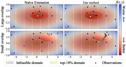
Figure 2: Scatter plots of observations obtained by the naïve extension (Left column) and our c-TPE (Right column) on a large (Top row, $z=0.5$) or small (Bottom row, $z=2.3$) overlap between the top-$10\%$ domain and feasible domain. Each figure shows the 2D search space for each task and the observations obtained during optimization are plotted. Earlier observations are colored black and later observations are colored white. Each figure has $50$ observations.

4 Experiments

Table 1: The table shows (Wins/Loses/Ties) of c-TPE against each method for optimizations with different constraint levels ($9$ benchmarks $\times$ $3$ constraint choices $=$ $27$ settings). The number of wins was counted by comparing medians of performance over $50$ random seeds in each setting between two methods. Non-bold numbers indicate $p<0.01$ of the hypothesis “The other method is better than c-TPE” by the Wilcoxon signed-rank test.

Quantiles $\gamma_{i}^{\mathrm{true}}=0.1$ $\gamma_{i}^{\mathrm{true}}=0.5$ $\gamma_{i}^{\mathrm{true}}=0.9$ Methods / # of configs 50 100 150 200 50 100 150 200 50 100 150 200 Naïve c-TPE 26/0/1 27/0/0 27/0/0 27/0/0 25/0/2 25/0/2 25/1/1 25/0/2 21/5/1 23/1/3 21/1/5 24/1/2 Vanilla TPE 27/0/0 27/0/0 27/0/0 27/0/0 25/0/2 26/0/1 26/1/0 24/0/3 14/11/2 18/8/1 15/5/7 16/7/4 Random 25/0/2 26/1/0 27/0/0 27/0/0 27/0/0 26/0/1 26/0/1 27/0/0 27/0/0 27/0/0 27/0/0 27/0/0 CNSGA-II 25/0/2 27/0/0 24/0/3 24/0/3 26/0/1 26/0/1 26/0/1 25/0/2 26/1/0 27/0/0 27/0/0 26/0/1 NEI 24/1/2 27/0/0 27/0/0 27/0/0 27/0/0 26/0/1 26/0/1 27/0/0 27/0/0 27/0/0 27/0/0 27/0/0 HM2 23/2/2 26/1/0 25/2/0 25/2/0 22/3/2 23/2/2 25/1/1 23/0/4 27/0/0 27/0/0 23/0/4 26/0/1

4.1 Setup

The evaluations were performed on the following $10$ tabular benchmarks:

1. HPOlib (Slice Localization, Naval Propulsion, Parkinsons Telemonitoring, Protein Structure) Klein and Hutter (2019): All with $6$ numerical and $3$ categorical parameters;

2. NAS-Bench-101 (CIFAR10A, CIFAR10B, CIFAR10C) Ying et al. (2019): Each with $26$ categorical, $14$ categorical, and $22$ numerical and $5$ categorical parameters, respectively; and

3. NAS-Bench-201 (ImageNet16-120, CIFAR10, CIFAR100) Dong and Yang (2020): All with $6$ categorical parameters.

The reason behind this choice is that tabular benchmarks enable us to control the quantiles of each constraint $\gamma_{i}^{\mathrm{true}}$, which significantly change the feasible domain size and the quality of solutions. For example, suppose a tabular dataset has $N_{\mathrm{all}}$ configurations $\{(\bm{x}_{n},f_{n},\bm{c}_{n})\}_{n=1}^{N_{\mathrm{all}}}$ and the dataset is sorted so that it satisfies $c_{i,1}\leq c_{i,2}\leq\dots\leq c_{i,N_{\mathrm{all}}}$ where $c_{i,n}$ is the $i$-th constraint value in the $n$-th configuration, then we fix the threshold for the $i$-th constraint $c_{i}^{\star}$ as $c_{i,\lfloor N_{\mathrm{all}}/10\rfloor}$ in the setting of $\gamma_{i}^{\mathrm{true}}=1/10$. We evaluated each benchmark with $9$ different quantiles $\gamma_{i}^{\mathrm{true}}$ for each constraint and $3$ different constraint choices. Constraint choices are network size, runtime, or both. The search space for each benchmark followed Awad et al. Awad et al. (2021).

As the baseline methods, we chose:

1. Random search Bergstra and Bengio (2012),

2. CNSGA-II Deb et al. (2002), (population size 8),

3. Noisy ECI (NEI) Letham et al. (2019) ,

4. Hypermapper2.0 (HM2) Nardi et al. (2019)  ,

5. Vanilla TPE (Optimize only loss as if we do not have constraints), and

6. Naïve c-TPE (The naïve extension discussed in Section 3).

We describe the details of each method and their control parameters in Appendix G. Note that all experiments were performed $50$ times with different random seeds and we evaluated $200$ configurations for each optimization. Additionally, since the optimizations by NEI and HM2 on CIFAR10C failed due to the high-dimensional ($22$ dimensions) continuous search space for NEI and an unknown internal issue for HM2, we used the results on $9$ benchmarks (other than CIFAR10C) for the statistical test and the average rank computation. The results on CIFAR10C by the other methods are available in Appendix H and the source code is available at https://github.com/nabenabe0928/constrained-tpe along with complete scripts to reproduce the experiments, tables, and figures. A query of c-TPE with $\{50,100,150,200\}$ observations took $\{0.22,0.24,0.26,0.28\}$ seconds for a 30D problem with 8 cores of core i7-10700.

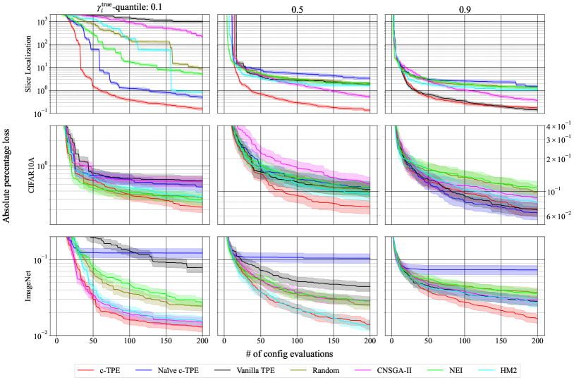
Figure 3: The performance curves on Slice Localization in HPOlib (Top row), CIFAR10A in NAS-Bench-101 (Middle row), and ImageNet16-120 in NAS-Bench-201 (Bottom row) with constraints of runtime and network size. We picked $\gamma_{i}^{\mathrm{true}}=0.1$ (Left column), $0.5$ (Center column), $0.9$ (Right column). The vertical axis shows the absolute percentage loss $(f_{\mathrm{observed}}-f_{\mathrm{oracle}})/f_{\mathrm{oracle}}$ where $f_{\mathrm{oracle}}$ is determined by looking up all feasible configurations in each benchmark. Note that each row shares the vertical axis except NAS-Bench-101. For $\gamma_{i}^{\mathrm{true}}=0.1$ in NAS-Bench-101, we separately scaled for the readability. Further results are available in Appendix H.

Table 2: The table shows (Wins/Loses/Ties) of c-TPE against each method for optimizations with different constraints ($9$ benchmarks $\times$ $9$ quantiles $=$ $81$ settings). The number of wins was counted by comparing medians of performance over $50$ random seeds in each setting between two methods. In this table, All results indicate $p<0.01$ of the hypothesis “The other method is better than c-TPE” by the Wilcoxon signed-rank test.

Constraints Runtime & Network size Network size Runtime Methods / # of configs 50 100 150 200 50 100 150 200 50 100 150 200 Naïve c-TPE 77/3/1 79/0/2 78/0/3 79/0/2 75/4/2 77/1/3 76/1/4 80/0/1 66/8/7 71/5/5 70/3/8 69/2/10 Vanilla TPE 73/7/1 75/5/1 72/3/6 73/4/4 69/10/2 74/6/1 74/3/4 72/6/3 62/12/7 67/10/4 62/6/13 60/9/12 Random 80/0/1 81/0/0 81/0/0 80/0/1 80/0/1 79/2/0 80/1/0 81/0/0 80/0/1 78/0/3 79/0/2 81/0/0 CNSGA-II 80/0/1 79/0/2 76/1/4 75/2/4 77/3/1 78/1/2 75/2/4 75/1/5 74/1/6 76/0/5 74/0/7 74/0/7 NEI 79/1/1 81/0/0 81/0/0 81/0/0 79/1/1 80/1/0 80/1/0 81/0/0 77/0/4 78/0/3 79/0/2 81/0/0 HM2 74/5/2 77/3/1 77/1/3 76/2/3 76/4/1 78/2/1 76/2/3 78/0/3 71/4/6 73/2/6 67/3/11 70/2/9

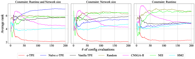
Figure 4: The average rank of each method over the number of evaluations. The horizontal axis shows the number of evaluated configurations in optimizations and the vertical axis shows the average rank over 81 settings. The title of each figure shows the constraint that the optimizations handled.

4.2 Robustness to Feasible Domain Size

This experiment shows how c-TPE performance improves given various levels of constraints. We optimized each benchmark with the aforementioned three types of constraints and chose $\gamma_{i}^{\mathrm{true}}\in\{0.1,0.5,0.9\}$ for each constraint. All results on other benchmarks are available in Appendix H. Table 1 presents the numbers of wins/loses/ties and statistical significance by the Wilcoxon signed-rank test and Figure 3 shows the performance curves for each benchmark.

As a whole, while the performance of c-TPE is stable across all constraint levels, that of NEI, HM2, and CNSGA-II variates depending on constraint levels. Furthermore, Table 1 shows that c-TPE is significantly better than other methods in almost all settings. This experimentally validates the robustness of c-TPE to the variations in constraint levels.

For ImageNet of NAS-Bench-201 (Bottom row), the naïve c-TPE is completely defeated by the other methods while c-TPE achieves the best or indistinguishable performance from the best performance. This gap between c-TPE and the naïve c-TPE is caused by the small overlaps discussed in Section 3.2.3. For example, only $59\%$ of the top-$10\%$ configurations belong to the feasible domain in NAS-Bench-201 of $\gamma_{i}^{\mathrm{true}}=0.9$ although we can usually expect that $90\%$ of them belong to the feasible domain, and $84\%$ and $77\%$ of those in HPOlib and NAS-Bench-101 actually belong to the feasible domain for $\gamma_{i}^{\mathrm{true}}=0.9$, respectively. The small overlap leads to the performance gap between c-TPE and the vanilla TPE as well. As TPE is not a uniform sampler and tries to sample from top domains, $\hat{\gamma}_{i}$ will not necessarily approach $\gamma_{i}^{\mathrm{true}}$. In our case, it is natural to consider $\hat{\gamma}_{i}$ to be closer to $59\%$ rather than $90\%$ as only $59\%$ of top-$10\%$ configurations are feasible. As mentioned also in Theorem 1, c-TPE is advantageous to such settings compared to the vanilla TPE and the naïve c-TPE.

For CIFAR10A of NAS-Bench-101 (Middle row), the results show different patterns from the other settings due to the high-dimensional ($D=26$) nature. For $\gamma_{i}^{\mathrm{true}}=0.1,0.5$ (Left, center), most methods exhibit indistinguishable performance from random search especially in the beginning because little information on feasible domains is available in the early stage of optimizations due to the high dimensionality although c-TPE outperforms in the end. In $\gamma_{i}^{\mathrm{true}}=0.9$ (Right), the naïve c-TPE is slightly better than c-TPE due to large overlaps ($84\%$ of the top-$10\%$ configurations are feasible). It implies that if search space is high dimensions and overlaps in top domains and feasible domains are large, it might be better to greedily optimize only the objective rather than regularizing the optimization of the objective as in our modification.

For Slice Localization of HPOlib (Top row), c-TPE outperforms the other methods. Furthermore, its performance almost coincides with that of the vanilla TPE in $\gamma_{i}^{\mathrm{true}}=0.9$ and it implies that our method gradually decays the priority of each constraint as $\gamma_{i}^{\mathrm{true}}$ becomes larger. In fact, the naïve c-TPE does not exhibit stability when the constraint level changes as it does not consider the priority of each constraint and the objective. This result empirically validates Theorem 1.

4.3 Average Rank over Number of Evaluations

This experiment demonstrates how c-TPE performance improves compared to the other methods over the number of evaluations. Table 2 presents the numbers of wins/loses/ties and statistical significance by the Wilcoxon signed-rank test and Figure 4 shows the average rank over $81$ settings ($9$ benchmarks $\times$ $9$ quantiles).

According to Figure 4, c-TPE quickly takes the top and keeps the rank until the end. From the figures, we can see that CNSGA-II improves in rank as the number of evaluations grows. In fact, since such slow-starting is often the case for evolutionary algorithms such as CMA-ES Loshchilov and Hutter (2016), the quick convergence achieved by c-TPE is appealing. For the multiple-constraint setting (Right), while the naïve c-TPE is worse than random search due to the small overlap, c-TPE overcomes this problem as discussed in Section 3.2.3. Table 2 confirmed the anytime performance of c-TPE by the statistical test over all the settings. All results on individual settings and quantile-wise average rank are available in Appendices H and I.

5 Related Work & Discussion

ECI was introduced by Gardner et al. Gardner et al. (2014) and Gelbart et al. Gelbart et al. (2014). Furthermore, there are various extensions of these prior works. For example, NEI is more robust to the noise caused in experiments Letham et al. (2019) and SCBO is scalable to high dimensions Eriksson and Poloczek (2021). Another technique for constrained BO is entropy search, such as predictive entropy search Lobato et al. (2015); Garrido-Merchán et al. (2023) and max-value entropy search Perrone et al. (2019). They choose the next configuration by approximating the expected information gain on the value of the constrained minimizer. While entropy search could outperform c-TPE on multimodal functions by leveraging the global search nature, slow convergence due to the global search nature and the expensive query cost hinder practical usages. Note that as the implementations of these methods are not provided in the aforementioned papers except NEI, we used only NEI in the experiments. The major advantages of TPE over standard GP-based BOs, used by all of these papers, are more natural handling of categorical and conditional parameters (see Appendix F) and easier integration of cheap-to-evaluate partial observations due to the linear time complexity with respect to $|\mathcal{D}|$. The concept of the integration of partial observations and its results, which showed a further acceleration of c-TPE, are available in Appendix C.

Also in the evolutionary algorithm (EA) community, constrained optimization has been studied actively, such as genetic algorithms (e.g. CNSGA-II Deb et al. (2002)), CMA-ES Arnold and Hansen (2012), or differential evolution Montes et al. (2006). Although CMA-ES has demonstrated the best performance among more than 100 methods for various black-box optimization problems Loshchilov et al. (2013), it does not support categorical parameters, so we did not include it in our experiments. Furthermore, since EAs have many control parameters, such as mutation rate and population size, meta-tuning may be necessary. Another downside of EAs is that it is hard to integrate partial observations because EAs require all the metrics to rank each configuration at each iteration. In general, BO overcomes these difficulties as discussed in Appendix C.

6 Conclusion

In this paper, we introduced c-TPE, a new constrained BO method. Although the AF of constrained BO and TPE could naturally come together using Corollary 1, such a naïve extension fails in some circumstances as discussed in Section 3. Based on the discussion, we modified c-TPE so that the formulation strictly generalizes TPE and falls back to it in settings of loose constraints. Furthermore, we empirically demonstrated that our modifications help to guide c-TPE to overlaps in the top and feasible domains. In our series of experiments on $9$ tabular benchmarks and with $27$ constraint settings, we first showed that the performance of c-TPE is not degraded over various constraint levels while the other BO methods we evaluated (HM2 and NEI) degraded as constraints became looser. Furthermore, the proposed method outperformed the other methods with statistical significance; however, since we focus only on the tabular benchmarks to enable the stability analysis of the performance variations depending on constraint levels, we discuss other possible situations where c-TPE might not perform well in Appendix E. Since TPE is very versatile and prominently used in several active OSS tools, such as Optuna and Ray, c-TPE will yield direct positive impact to practitioners in the future.

Appendix A Proofs

A.1 Preliminaries

We use the following definitions to make the discussion of constraint levels simpler:

Definition 1 ($\gamma$-quantile value)

Given a quantile $\gamma\in(0,1]$ and a measurable function $f\mathrm{:}~{}\mathcal{X}\rightarrow\mathbb{R}$, $\gamma$-quantile value $f^{\gamma}\in\mathbb{R}$ is a real number such that$\mathrm{:}$

$$f^{\gamma}\coloneqq\inf\biggl{\{}f^{\star}\in\mathbb{R}~{}\biggl{|}\int_{\bm{x}\in\mathcal{X}}\mathbbm{1}[f(\bm{x})\leq f^{\star}]\frac{\mu(d\bm{x})}{\mu(\mathcal{X})}\geq\gamma\biggr{\}}.$$ (13)

where $\mu$ is the Lebesgue measure on $\mathcal{X}$.

Definition 2

Given a constraint $c~{}\!\mathrm{:}~{}\mathcal{X}\rightarrow\mathbb{R}$ and a constraint threshold $c^{\star}\in\mathbb{R}$, ${\gamma_{c^{\star}}}$ is defined as the quantile of the constraint $c$ such that $c^{\star}=c^{\gamma_{c^{\star}}}$.

Definition 3 ($\Gamma$-feasible domain)

Given a set of constraint thresholds $c_{i}^{\star}\in\mathbb{R}$ $\mathrm{(}$for $i\in\{1,\dots,C\}\mathrm{)}$, we define the feasible domain $\mathcal{X}^{\prime}=\{\bm{x}\in\mathcal{X}|\forall i,c_{i}(\mathcal{X})\leq c_{i}^{\star}\}$. Then the feasible domain ratio is computed as $\Gamma=\mu(\mathcal{X}^{\prime})/\mu(\mathcal{X})\in(0,1]$ and the domain is said to be the $\Gamma$-feasible domain.

Note that $\bm{x}\in\mathbb{R}^{D}$ is a hyperparameter configuration, $\mathcal{X}=\mathcal{X}_{1}\times\dots\times\mathcal{X}_{D}\subseteq\mathbb{R}^{D}$ is the search space of the hyperparameter configurations, $\mathcal{X}_{d}\subseteq\mathbb{R}~{}(\text{for }d=1,\dots,D)$ is the domain of the $d$-th hyperparameter, Note that we consider two assumptions mentioned in Appendix A.2 and those assumptions allow the whole discussion to be extended to search spaces with categorical parameters.

A.2 Assumptions

In this paper, we assume the following:

1. Objective $f:\mathcal{X}\rightarrow\mathbb{R}$ and constraints $c_{i}:\mathcal{X}\rightarrow\mathbb{R}$ are Lebesgue integrable and are measurable functions defined over the compact measurable subset $\mathcal{X}\subseteq\mathbb{R}^{D}$,

2. The support of PI for the objective $\mathbb{P}(f\leq f^{\star}|\mathcal{X},\mathcal{D})$ and each constraint $\mathbb{P}(c_{i}\leq c_{i}^{\star}|\bm{x},\mathcal{D})$ covers the whole domain $\mathcal{X}$ for an arbitrary choice of $f^{\star},c_{i}^{\star}\in\mathbb{R}$,

where $\mathcal{D}=\{(\bm{x}_{n},f_{n},\bm{c}_{n})\}_{n=1}^{N}$ is a set of observations, and $\bm{c}_{n}=[c_{1,n},\dots,c_{C,n}]\in\mathbb{R}^{C}$ is the $n$-th observation of each constraint. The Lebesgue integrability easily holds for TPE as TPE only considers the order of each configuration and almost all functions are measurable unless they are constructive. Note that we also assume a categorical parameter to be $\mathcal{X}_{i}=[1,K]$ as in the TPE implementation bergstra2011algorithms where $K$ is a number of categories. As we do not require the continuity of $f$ and $c_{i}$ with respect to hyperparameters in our analysis, this definition is valid as long as the employed kernel for categorical parameters treats different categories to be equally similar such as Aitchison-Aitken Kernel aitchison1976multivariate. In this definition, $x,x^{\prime}\in\mathcal{X}_{i}$ are viewed as equivalent as long as $\lfloor x\rfloor=\lfloor x^{\prime}\rfloor$ and it leads to the random sampling of each category to be uniform and the Lebesgue measure of $\mathcal{X}$ to be non-zero.

A.3 Proof of Proposition 1

Proof 1

Using $\mathrm{Eq.}~{}(\ref{eq:l-and-g-trick})$, $\mathrm{PI}$ is computed as$\mathrm{:}$

$$\mathbb{P}(f\leq f^{\star}\mid\bm{x},\mathcal{D}) =\int_{-\infty}^{f^{\star}}p(f|\bm{x},\mathcal{D})df$$

$$=\int_{-\infty}^{f^{\star}}\frac{p(\bm{x}|f,\mathcal{D})p(f|\mathcal{D})}{p(\bm{x}|\mathcal{D})}df$$

$$=\frac{p(\bm{x}|\mathcal{D}^{(l)})}{p(\bm{x}|\mathcal{D})}\int_{-\infty}^{f^{\star}}p(f|\mathcal{D})df.$$

Notice that $\mathcal{D}$ is split by $f^{\star}$. $\mathrm{EI}$ in $\mathrm{TPE}$ is computed as$\mathrm{:}$

$$\mathrm{EI}_{f^{\star}}[\bm{x}|\mathcal{D}] =\frac{p(\bm{x}|\mathcal{D}^{(l)})}{p(\bm{x}|\mathcal{D})}\int_{-\infty}^{f^{\star}}(f^{\star}-f)p(f|\mathcal{D})df.$$ (15)

When we take the ratio of $\mathrm{Eqs}~{}(\ref{appx:proof:eq:pi-form}),(\ref{appx:proof:eq:ei-form})$, the part that depends on $\bm{x}$ cancels out as follows$\mathrm{:}$

$$\frac{\int_{-\infty}^{f^{\star}}(f^{\star}-f)p(f|\mathcal{D})df}{\int_{-\infty}^{f^{\star}}p(f|\mathcal{D})df}=\mathrm{const~{}w.r.t.}~{}\bm{x},$$ (16)

where, since we assume that the support of $\mathbb{P}(f\leq f^{\star}|\bm{x},\mathcal{D})$ covers the whole domain $\mathcal{X}$, i.e. $\forall\bm{x}\in\mathcal{X},\mathbb{P}(f\leq f^{\star}|\bm{x},\mathcal{D})\neq 0$ and $f$ is Lebesgue integrable, i.e. the expectation of $f$ exists and $\int|f|\mu(d\bm{x})<\infty$, both numerator and denominator always take a positive finite value, and thus the $\mathrm{LHS}$ of $\mathrm{Eq.}~{}(\ref{ratio-of-ei-and-pi-is-constant})$ takes a finite positive constant value.

A.4 Proof of Corollary 1

Proof 2

Under the $\mathrm{TPE}$ formulation, $\mathrm{EI}_{f^{\star}}(\bm{x}|\mathcal{D})$ is proportional to $r^{\mathrm{rel}}_{0}(\bm{x}|\mathcal{D})$ and $\mathrm{EI}_{c_{i}^{\star}}(\bm{x}|\mathcal{D})$ is proportional to $r^{\mathrm{rel}}_{i}(\bm{x}|\mathcal{D})$ as shown by Bergstra et al. Bergstra et al. (2011). Furthermore, since $\mathrm{EI}$ and $\mathrm{PI}$ are equivalent in the $\mathrm{TPE}$ formulation from Proposition 1, $\mathrm{ECI}$ for $\mathrm{TPE}$ satisfies the following using $\mathrm{Eq.~{}(\ref{main:method:eq:eci-transformation-derivation})}$:

$$\mathrm{ECI}_{f^{\star}}[\bm{x}|\bm{c}^{\star},\mathcal{D}] \propto\mathbb{P}(f\leq f^{\star}|\bm{x},\mathcal{D})\prod_{i=1}^{C}\mathbb{P}(c_{i}\leq c_{i}^{\star}|\bm{x},\mathcal{D})$$ (17)

$$\propto\prod_{i=0}^{C}r^{\mathrm{rel}}_{i}(\bm{x}|\mathcal{D}).$$

This completes the proof.

A.5 Proof of Theorem 1

Proof 3

From $\mathrm{Corollary~{}\ref{main:method:proof:eci-is-product-of-relative-density-ratios}}$, since $\mathrm{ECI}_{f^{\star}}[\bm{x}|\bm{c}^{\star},\mathcal{D}]\propto\prod_{k=0}^{C}r^{\mathrm{rel}}_{k}$ holds, the partial derivative of the $\mathrm{RHS}$ with respect to the density ratio $r_{k}(\bm{x})$ for $k\in\{0,\dots,C\}$ is computed as follows$\mathrm{:}$

$$\frac{\partial\mathrm{ECI}_{f^{\star}}[\bm{x}|\bm{c}^{\star},\mathcal{D}]}{\partial r_{k}} \propto\frac{\partial r^{\mathrm{rel}}_{k}}{\partial r_{k}}\prod_{k^{\prime}\neq k}r^{\mathrm{rel}}_{k^{\prime}}$$

$$=\frac{\partial}{\partial r_{k}}\frac{1}{\hat{\gamma}_{k}+(1-\hat{\gamma}_{k})r_{k}^{-1}}\prod_{k^{\prime}\neq k}r^{\mathrm{rel}}_{k^{\prime}}$$

$$=\frac{1-\hat{\gamma}_{k}}{(\hat{\gamma}_{k}r_{k}+1-\hat{\gamma}_{k})^{2}}\prod_{k^{\prime}\neq k}r^{\mathrm{rel}}_{k^{\prime}}$$ (18)

$$=\frac{1-\hat{\gamma}_{k}}{r_{k}^{2}}r^{\mathrm{rel}}_{k}\prod_{k^{\prime}=0}^{C}r^{\mathrm{rel}}_{k^{\prime}}\geq 0$$

$$(\because\forall k^{\prime}\in\{0,\dots,C\}, r_{k^{\prime}},r^{\mathrm{rel}}_{k^{\prime}}>0,0\leq 1-\hat{\gamma}_{k}<1).$$

For this reason, the $\mathrm{LHS}$ takes zero if and only if $\hat{\gamma}_{k}=1$. Using the result, the following holds with a positive constant number $\alpha$$\mathrm{:}$

$$\frac{\partial\mathrm{ECI}_{f^{\star}}[\bm{x}|\bm{c}^{\star},\mathcal{D}]}{\partial r_{i}}-\frac{\partial\mathrm{ECI}_{f^{\star}}[\bm{x}|\bm{c}^{\star},\mathcal{D}]}{\partial r_{j}}$$ (19)

$$=\alpha\Biggl{(}\frac{1-\hat{\gamma}_{i}}{r_{i}^{2}}r^{\mathrm{rel}}_{i}-\frac{1-\hat{\gamma}_{j}}{r_{j}^{2}}r^{\mathrm{rel}}_{j}\Biggr{)}$$

$$=\alpha\Biggl{(}\frac{1-\hat{\gamma}_{i}}{\hat{\gamma}_{i}r_{i}^{2}+(1-\hat{\gamma}_{i})r_{i}}-\frac{1-\hat{\gamma}_{j}}{\hat{\gamma}_{j}r_{j}^{2}+(1-\hat{\gamma}_{j})r_{j}}\Biggr{)}$$

$$=\alpha\Biggl{(}\biggl{(}r_{i}+\frac{\hat{\gamma}_{i}}{1-\hat{\gamma}_{i}}r_{i}^{2}\biggr{)}^{-1}-\biggl{(}r_{j}+\frac{\hat{\gamma}_{j}}{1-\hat{\gamma}_{j}}r_{j}^{2}\biggr{)}^{-1}\Biggr{)}.$$

Since $r_{i},r_{j}>0$ holds and

$$r_{i}+\frac{\hat{\gamma}_{i}}{1-\hat{\gamma}_{i}}r_{i}^{2}\geq r_{j}+\frac{\hat{\gamma}_{j}}{1-\hat{\gamma}_{j}}r_{j}^{2},$$ (20)

$$\frac{\partial\mathrm{ECI}_{f^{\star}}[\bm{x}|\bm{c}^{\star},\mathcal{D}]}{\partial r_{i}}-\frac{\partial\mathrm{ECI}_{f^{\star}}[\bm{x}|\bm{c}^{\star},\mathcal{D}]}{\partial r_{j}}$$ (21)

$$=\alpha\Biggl{(}\biggl{(}r_{i}+\frac{\hat{\gamma}_{i}}{1-\hat{\gamma}_{i}}r_{i}^{2}\biggr{)}^{-1}-\biggl{(}r_{j}+\frac{\hat{\gamma}_{j}}{1-\hat{\gamma}_{j}}r_{j}^{2}\biggr{)}^{-1}\Biggr{)}\geq 0$$

holds. When we assume $\hat{\gamma}_{i}=\hat{\gamma}_{j}$ and $r_{i}=r_{j}$, we get the equality. This completes the proof.

Note that since $x/(1-x)$ is a monotonically increasing function in $x\in[0,1)$ and $\hat{\gamma}_{i}\leq\hat{\gamma}_{j}$ from the assumption,

$$0\leq\alpha_{i}\coloneqq\frac{\hat{\gamma}_{i}}{1-\hat{\gamma}_{i}}\leq\alpha_{j}\coloneqq\frac{\hat{\gamma}_{j}}{1-\hat{\gamma}_{j}}$$ (22)

holds. Furthermore, using $r_{i},r_{j}>0$, if we assume $r_{i}<r_{j}$, then $r_{i}<r_{j},r_{i}^{2}<r_{j}^{2},\alpha_{i}<\alpha_{j}$ and it leads to a larger value of partial derivative in the $i$-th constraint; therefore, $r_{j}$ must be smaller than $r_{i}$ for its contribution to be larger than that from $r_{i}$. It implies that we will not put more priority on the constraints with large feasible domains unless those constraints are likely to be violated, which means the density ratios for those constraints are small.

A.6 Proof of Corollary 2

To prove Corollary 2, we first show two lemmas.

Lemma 1

Given a $\Gamma$-feasible domain ($\Gamma>0$) with constraint thresholds of $c_{i}^{\star}$ for all $i\in\{1,\dots,C\}$, each constraint satisfies

$$\forall i\in\{1,\dots,C\},\gamma_{i}\geq\Gamma.$$ (23)

Proof 4

Let the feasible domain for the $i$-th constraint be $\mathcal{X}^{\prime}_{i}=\{\bm{x}\in\mathcal{X}|c_{i}\leq c_{i}^{\star}\}$. Then the feasible domain is $\mathcal{X}^{\prime}=\bigcap_{i=1}^{C}\mathcal{X}^{\prime}_{i}$. Since $\mathcal{X}^{\prime}_{i}$ is a measurable set by definition and $\mathcal{X}^{\prime}\subseteq\mathcal{X}_{i}^{\prime}$ holds, $\Gamma/\gamma_{i}=\mu(\mathcal{X}^{\prime})/\mu(\mathcal{X}^{\prime}_{i})\leq 1$ holds. $\Gamma$ is a positive number, so $\gamma_{i}\geq\Gamma$ and this completes the proof.

Lemma 2

The domain is $\mathrm{(}\Gamma=1\mathrm{)}$-feasible domain iff:

$$\forall i\in\{1,\dots,C\},\gamma_{i}=1.$$ (24)

Proof 5

Suppose $\gamma_{i}<1$ for some $i\in\{1,\dots,C\}$, since we immediately obtain $\Gamma\leq\gamma_{i}<1$ from $\mathrm{Lemma~{}\ref{lemma-c-gamma-is-larger-than-gamma}}$, the assumption does not hold. For this reason, $\gamma_{i}\geq 1$ for all $i\in\{1,\dots,C\}$ and since $\gamma_{i}\leq 1$ by definition, $\gamma_{i}=1$ for all $i\in\{1,\dots,C\}$. Since $\mathcal{X}_{i}^{\prime}=\mathcal{X}$ for all $i\in\{1,\dots,C\}$, $\bigcup_{i=1}^{C}\mathcal{X}_{i}^{\prime}=\bigcup_{i=1}^{C}\mathcal{X}=\mathcal{X}$ holds. This completes the proof.

Using Lemma 24 and Theorem 1, we prove Corollary 2.

Proof 6

From $\mathrm{Lemma~{}\ref{all-gamma-must-be-one}}$, when $\Gamma=1$ holds, $\gamma_{i}=1$ for all $i\in\{1,\dots,C\}$ holds, and we plug $\gamma_{i}=1$ into $\mathrm{Theorem~{}\ref{main:vanished-constraints:thm:tight-constraint-have-more-priority}}$. Then we obtain$\mathrm{:}$

$$\forall i\in\{1,\dots,C\},\frac{\partial\mathrm{ECI}_{f^{\star}}[\bm{x}|\bm{c}^{\star},\mathcal{D}]}{\partial r_{i}}=0.$$ (25)

For this reason, $\mathrm{ECI}_{f^{\star}}[\bm{x}|\bm{c}^{\star},\mathcal{D}]\propto\prod_{i=0}^{C}r^{\mathrm{rel}}_{i}(\bm{x}|\mathcal{D})\propto r^{\mathrm{rel}}_{0}(\bm{x}|\mathcal{D})\stackrel{{\scriptstyle\mathrm{rank}}}{{\simeq}}r_{0}(\bm{x}|\mathcal{D})$ and this completes the proof.

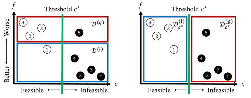
Figure 5: The conceptual visualizations of the split algorithm for the objective and for each constraint. The black and white circles represent infeasible and feasible solutions, respectively. The numberings for white and black circles stand for the ranking of the objective value among feasible and infeasible solutions, respectively. The configurations enclosed by the red and blue rectangles belong to the bad and good groups, respectively. Left: the split for the objective. While the original algorithm is supposed to take only the black circle (infeasible solution) with 1 ($=\lceil\sqrt{9}/4\rceil$) for the good group, our algorithm takes until the white circle (feasible solution) with 1, and thus we include the black circles till 4 as well. Right: the split for the constraint. Our algorithm takes all white circles (feasible solutions).

Figure 6: The visualization of the observations obtained by c-TPE and the vanilla TPE on ImageNet16-120 of NAS-Bench-201 with $\gamma_{i}^{\mathrm{true}}=0.1$. Each optimization was run $5$ times. The red and blue dots are infeasible and feasible solutions, respectively. The left side of the threshold (green line) is the feasible domain. The goal is to find configurations near the oracle (purple line) in the feasible domain. Left: the optimization by c-TPE. Red dots (infeasible solutions) locate relatively close to the threshold (green line). Right: the optimization by the vanilla TPE. Since red dots (infeasible solutions) locate far away from the threshold (green line), it cannot intensively search near the threshold.

Appendix B Further Details of Split Algorithms

In this section, we describe the intuition and more details on how the split algorithm works.

B.1 Split Algorithm of Objective

Figure 5 presents how to split observations into good and bad groups. For the split for the objective (Left), as there are $N=9$ observations, we will include $\lceil\sqrt{N}/4\rceil=\lceil\sqrt{9}/4\rceil=1$ feasible solution in $\mathcal{D}^{(l)}$. We first find the feasible observation with the best objective value, which is the white-circled observation 1. Then $\mathcal{D}^{(l)}_{0}$ and $\mathcal{D}^{(g)}_{0}$ are obtained by splitting the observations at the white observation 1 along the horizontal axis. As discussed in Section 3.2.3, this modification is effective for small overlaps and small overlaps are caused by observations with the best objective values far away from the feasible domain, e.g. the black-circled observations 1 and 3 in Figure 5. For example, Figure 6 visualizes the observations by c-TPE and the vanilla TPE on ImageNet16-120 of NAS-Bench-201 with $\gamma_{i}^{\mathrm{true}}=0.1$. There are many observations with strong performance than the oracle (purple line) that are far from the feasible domain (left side of the green line) in the result of the vanilla TPE. Note that the oracle is the best objective value that satisfies the constraint. Theorem 1 guarantees that c-TPE will not prioritizes such observations.

B.2 Split Algorithm of Each Constraint

We first note that we show, for simplicity, a 1D example and abbreviate $c_{i},c_{i}^{\star},\mathcal{D}^{(l)}_{i},\mathcal{D}^{(g)}_{i}$ as $c,c^{\star},\mathcal{D}^{(l)}_{c^{\star}},\mathcal{D}^{(g)}_{c^{\star}}$, respectively. For the split of each constraint (Right), we take the observations with constraint values less than $c^{\star}$ into $\mathcal{D}^{(l)}_{c^{\star}}$ (inside the blue rectangle) and vice versa. When there are no observations in the feasible domain, we only take the observation with the best constraint value among all the observations into $\mathcal{D}^{(l)}_{c^{\star}}$ and the rest into $\mathcal{D}^{(g)}_{c^{\star}}$. Since this selection increases the priority of this constraint as mentioned in Theorem 1, it raises the probability of yielding feasible solutions quickly.

Algorithm 2 c-TPE with knowledge augmentation

1:$N_{\mathrm{init}}$ (The number of initial configurations), $N_{s}$ (The number of candidates to consider in the optimization of the AF), $N_{p}$ (The number of configurations for KA) $\triangleright$ Control parameters

2:$I=\{i_{j}\}_{j=1}^{C_{p}}$ $\triangleright$ Indices of cheap constraints

3:$\mathcal{D}_{p}\leftarrow\emptyset,\mathcal{D}\leftarrow\emptyset$

4:for $n=1,\dots,N_{p}$ do $\triangleright$ Collect cheap information

5:     Randomly pick $\bm{x}$

6:     $\mathcal{D}_{p}\leftarrow\mathcal{D}_{p}\cup\{(\bm{x},f(\bm{x}),c_{i_{1}}(\bm{x}),\dots,c_{i_{C_{p}}}(\bm{x}))\}$

7:for $n=1,\dots,N_{\mathrm{init}}$ do

8:     Randomly pick $\bm{x}$

9:     $\mathcal{D}\leftarrow\mathcal{D}\cup\{(\bm{x},f(\bm{x}),c_{1}(\bm{x}),\dots,c_{C}(\bm{x}))\}$

10:while Budget is left do

11:     for $i=0,\dots,C$ do

12:         if $i\in I$ then

13:              $\mathcal{D}_{\text{aug}}=\mathcal{D}\cup\mathcal{D}_{p}$

14:         else

15:              $\mathcal{D}_{\text{aug}}=\mathcal{D}$          

16:         Split $\mathcal{D}_{\text{aug}}$ into $\mathcal{D}^{(l)}_{i}$ and $\mathcal{D}^{(g)}_{i}$, $\hat{\gamma}_{i}\leftarrow|\mathcal{D}^{(l)}_{i}|/|D_{\text{aug}}|$

17:         Build $p(\cdot|\mathcal{D}^{(l)}_{i}),p(\cdot|\mathcal{D}^{(g)}_{i})$

18:         $\{\bm{x}_{j}\}_{j=1}^{N_{s}}\sim p(\cdot|\mathcal{D}^{(l)}_{i}),\mathcal{S}\leftarrow\mathcal{S}\cup\{\bm{x}_{j}\}_{j=1}^{N_{s}}$      

19:     Pick $\bm{x}_{\mathrm{opt}}\in\mathop{\mathrm{argmax}}_{\bm{x}\in\mathcal{S}}\prod_{i=0}^{C}r^{\mathrm{rel}}_{i}(\bm{x}|\mathcal{D})$

20:     $\mathcal{D}\leftarrow\mathcal{D}\cup\{(\bm{x}_{\mathrm{opt}},f(\bm{x}_{\mathrm{opt}}),c_{1}(\bm{x}_{\mathrm{opt}}),\dots,c_{C}(\bm{x}_{\mathrm{opt}}))\}$

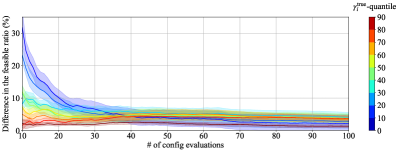
Figure 7: The effect of KA in the optimizations with a constraint for network size. The horizontal axis shows the number of evaluated configurations in optimizations and the vertical axis shows the difference in the cumulated ratio of feasible solutions, i.e. the ratio of the number of feasible solutions to that of the whole observations, between c-TPE and c-TPE with KA using 200 randomly sampled configurations. The weak-color bands show the standard error of mean values of 50 runs for 9 benchmarks.

Appendix C Integration of Partial Observations

In this section, we discuss the integration of partial observations for BO and we name the integration “Knowledge augmentation (KA)”.

C.1 Knowledge Augmentation

When some constraints can be precisely evaluated with a negligible amount of time compared to others, practitioners typically would like to use KA. For example, the network size of deep learning models is trivially computed in seconds while the final validation performance requires several hours to days. In this case, we can obtain many observations only for network size and augment the knowledge of network size prior to the optimization so that the constraint violations will be reduced in the early stage of optimizations.

To validate the effect of KA, all of the additional results in the appendix include the results obtained using c-TPE with KA. In the experiments, we augmented the knowledge only for network size and we did not include runtime as a target of KA because although runtime can be roughly estimated from a 1-epoch training, such estimations are not precise. However, practitioners can include such rough estimations into partial observations as long as they can accept errors caused by them.

C.2 Algorithm of Knowledge Augmentation

Algorithm 2 is the pseudocode of c-TPE with KA. We first need to specify a set of indices for cheap constraints $I=\{i_{j}\}_{j=1}^{C_{p}}$ where $C_{p}(<C)$ is the number of cheap constraints and $I\subseteq\{1,\dots,C\}$. In Lines 4 – 6, we first collect partial observations $\mathcal{D}_{p}$. Then we augment observations in Lines 12 – 15 if partial observations are available for the corresponding constraint. We denote the augmented set of observations $\mathcal{D}_{\mathrm{aug}}$. When the AF follows Eq. (10), the predictive models for each constraint are independently trained due to conditional independence. It enables us to introduce different amounts of observations for each constraint. Since c-TPE follows Eq. (10), we can employ KA. As discussed in Section 5, it is hard to apply KA to evolutionary algorithms due to their algorithm nature and KA causes a non-negligible bottleneck for GP-based BO as the number of observations grows.

C.3 Empirical Results of Knowledge Augmentation

In this experiment, we optimized each benchmark with a constraint for network size, and constraints for runtime and network size. To see the effect, we measured how much KA increases the chance of drawing feasible solutions and tested the performance difference by the Wilcoxon signed-rank test on 18 settings ($9$ benchmarks $\times$ $2$ constraint choices). According to Figure 7, the tighter the constraint becomes, the more KA helps to obtain feasible solutions, especially in the early stage of the optimizations. Additionally, Table 3 shows the statistically significant speedup effects of KA in $\gamma_{i}^{\mathrm{true}}=0.1$. Although KA did not exhibit the significant speedup in loose constraint levels, it did not deteriorate the optimization quality significantly. At the later stage of the optimizations, the effect gradually decays as c-TPE becomes competent enough to detect violations. In summary, KA significantly accelerates optimizations with tight constraints and it does not deteriorate the optimization quality in general, so it is practically recommended to use KA as much as possible.

Table 3: The table shows (Wins/Loses/Ties) of c-TPE with KA against c-TPE for optimizations with different constraint levels. Non-bold numbers indicate $p<0.05$ of the hypothesis “c-TPE is better than c-TPE with KA” by the Wilcoxon signed-rank test.

Quantiles	$\gamma_{i}^{\mathrm{true}}=0.1$				$\gamma_{i}^{\mathrm{true}}=0.5$				$\gamma_{i}^{\mathrm{true}}=0.9$
# of configs	50	100	150	200	50	100	150	200	50	100	150	200
Wins/Loses/Ties	12/5/1	11/5/2	7/5/6	6/6/6	6/12/0	5/11/2	7/6/5	5/5/8	9/9/0	10/6/2	8/5/5	6/9/3

Appendix D Hard-Constrained Optimization Problems

In this paper, although we only handled optimization problems with inequality constraints, c-TPE is applicable to optimization problems with a hard constraint, which practitioners often face in practice. For example, we are able to perform the training of a machine learning model with a hyperparameter configuration $\bm{x}$ only if the memory requirement is lower than the RAM capacity of the system. In this case, when the training with the hyperparameter configuration $\bm{x}$ fails, we only know that the hyperparameter configuration $\bm{x}$ does not satisfy the constraint and we do not yield either $f(\bm{x})$ or $c(\bm{x})$. Since we only need to be able to split observations into $\mathcal{D}^{(l)}_{i}$ and $\mathcal{D}^{(g)}_{i}$ with respect to the hard constraint, $\mathcal{D}^{(l)}_{i}$ will collect all observations that satisfy the hard constraint and $\mathcal{D}^{(g)}_{i}$ will collect the others. For the objective $f(\bm{x})$, we simply ignore all the observations that violate the hard constraint. As discussed in Appendix C, the surrogate model could be simply obtained even from a set of partial observations. In this problem setting, the feasible observations for the hard constraint $\mathcal{D}^{(l)}_{i}$ could often be an empty set and then $p(\bm{x}|\mathcal{D}^{(l)}_{i})$ becomes simply the non-informative prior employed in TPE watanabe2023tpe. As $p(\cdot|\mathcal{D}^{(g)}_{i})$ still provides the information about the violation of the hard constraint, c-TPE simply searches the regions far from the current violated observations.

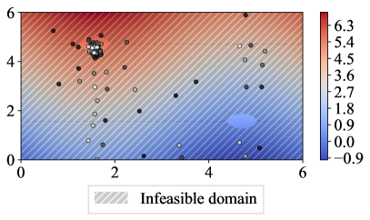
Figure 8: The optimization of Eq. (26) by c-TPE. Blue implies that the objective function is better and the shaded area is infeasible domain. Earlier observations are colored black and later observations are colored white. This figure has $100$ observations. Since this problem has two modals and each of them is very small, c-TPE was trapped by one of the two modals and could not escape from there within the specified number of observations.

Appendix E Limitations

In this paper, we focused on tabular benchmarks for search spaces with categorical parameters and with one or two constraints. We chose the tabular benchmarks to enable the stability analysis of the performance variations depending on constraint levels. Furthermore, such settings are common in HPO of deep learning. However, since practitioners may use c-TPE for other settings, we would like to discuss the following settings which we did not cover in the paper:

1. Extremely small feasible domain size,

2. Many constraints,

3. Parallel computation, and

4. Synthetic functions.

The first setting is an extremely small feasible domain size. For example, when we have $\Gamma=10^{-4}$ for $200$ evaluations and use random search, we will not get any feasible solutions with the probability of $(1-10^{-4})^{200}=0.9802\dots\simeq 98.0\%$. Such settings are generally hard for most optimizers to find even one feasible solution.

The second setting is tasks with many constraints. In our experiments, we have the constraints of runtime and network size. On the other hand, there might be more constraints in other purposes. Many constraints make the optimization harder because the feasible domain size becomes smaller as the number of constraints increases due to the curse of dimensionality. More formally, when we define the feasible domain for the $i$-th constraint as $\mathcal{X}_{i}^{\prime}=\{\bm{x}\in\mathcal{X}|c_{i}(\bm{x})\leq c_{i}^{\star}\}$, the feasible domain size shrinks exponentially unless some feasible domains are identical, i.e. $\mathcal{X}_{i}^{\prime}=\mathcal{X}_{j}^{\prime}$ for some pairs $(i,j)\in\{1,\dots,C\}\times\{1,\dots,C\}$ such that $i\neq j$. This setting is also generally hard due to the small feasible domain size.

The third setting is parallel computation. In HPO, since objective functions are usually expensive, it is often preferred to be able to optimize in parallel with less regret. For example, since evolutionary algorithms evaluate a fixed number $G$ of configurations in one generation, they optimize the objective function without any loss compared to the sequential setting up to $G$ parallel processes. Although TPE (and c-TPE) are applicable to asynchronous settings, we cannot conclude c-TPE works nicely in parallel settings from our experiments.

The fourth setting is synthetic function. We did not handle synthetic function because it is hard to prepare the exact $\gamma_{i}^{\mathrm{true}}$. As mentioned earlier, one of the most important points of our method is the robustness with respect to various constraint levels. As synthetic functions are designed to be hard in certain constraint thresholds, it was hard to maintain the difficulties for different $\gamma_{i}^{\mathrm{true}}$ and to even analytically compute $\gamma_{i}^{\mathrm{true}}$. It is worth noting that c-TPE is likely to not perform well on multi-modal functions. For example, Figure 8 presents such an instance. This example uses:

$$\min_{(x_{1},x_{2})\in[0,2\pi]\times[0,2\pi]} \sin x_{1}+x_{2}$$ (26)

$$\mathrm{subject~{}to~{}}\sin x_{1} \sin x_{2}\leq-0.95.$$

In this case, c-TPE was trapped in one of the two feasible domain where we have worse objective values. Since this case has small feasible domains and c-TPE searches locally due to the nature of PI, it intensively searches one of the feasible domains which c-TPE first finds and it is hard for c-TPE to find both of the two modals. In this example, c-TPE may require more evaluations to cover both modals compared to global search methods although this issue could be addressed by multiple runs of c-TPE.

Since we did not test c-TPE on those settings, practitioners are encouraged to compare c-TPE with other methods if their tasks of interest have the characteristics described above.

Appendix F Performance of Vanilla TPE

As described in Appendix G, since our TPE implementation uses multivariate kernel density estimation, it is different from the Hyperopt implementation that is used in most prior works. For this reason, we compare our the performance of our TPE implementation with that of Hyperopt, and other BO methods. Since all settings include categorical parameters, we compare the following BO methods which are known to perform well on search space with categorical parameters.

1. TuRBO eriksson2019scalable , and

2. CoCaBO ru2020bayesian .

CoCaBO is a BO method that focuses on the handling of categorical parameters and TuRBO is one of the strongest BO methods developed recently. Both methods follow the default settings. Note that as both methods are either not extended to constrained optimization or not publicly available, we could not include those methods in Section 4.

Figure 9 shows the average rank over time for each method. As seen in the figure, our TPE outperformed Hyperopt. Furthermore, while our TPE is significantly better than other methods in most settings, Hyperopt is better than only CoCaBO. On the other hand, TuRBO-1 performs better in the early stage of optimizations although our TPE outperforms TuRBO-1 with statistical significance, and this cold start in the vanilla TPE might be a trade-off. Notice that since most BO papers test performance on toy functions and we use the tabular benchmarks, the discussion here does not generalize and the results only validate why we should use our TPE in our paper.

Figure 9: The performance comparison of our TPE implementation against prior works and Hyperopt implementation. The horizontal axis represents the number of configurations and the vertical axis represents the average rank of each method over $9$ benchmarks that were used in Section 4.

Table 4: In the table, we show the test results of The hypothesis “The other method is better than our TPE” for the “v.s. our TPE” column and the hypothesis “The other method is better than Hyperopt” for the “v.s. Hyperopt” column by the Wilcoxon signed-rank test. For example, the “TuRBO-1” row in the “v.s. our TPE” column says “N/N/W/W”. It means while we cannot draw any conclusion about the performance difference with $50,100$ evaluations, TuRBO-1 is significantly worse than our TPE with $150,200$ evaluations in our settings. Note that we chose $p<0.01$ as the threshold. Each method was run over 15 random seeds.

Methods v.s. our TPE v.s. Hyperopt # of configs 50/100/150/200 50/100/150/200 our TPE –/–/–/– N/B/B/B Hyperopt N/W/W/W –/–/–/– TuRBO-1 N/N/W/W B/N/N/N TuRBO-5 W/W/W/W W/N/N/N CoCaBO W/W/W/W N/W/W/W

Appendix G Details of Experiment Setup

For all the methods using TPE, we used $N_{s}=24$ and $N_{\mathrm{init}}=10$, which we obtain from the ratio ($5\%$) of the initial sample size and the number of evaluations, as in the original paper bergstra2013making. Furthermore, we employed the multivariate kernel and its bandwidth selection used by the prior work falkner2018bohb. Due to this modification, our vanilla TPE implementation performs significantly better than Hyperopt bergstra2013making  on our experiment settings, and thus we would like to stress that our TPE may produce better results compared to what we can expect from prior works daxberger2019mixed,deshwal2021bayesian,eggensperger2013towards,ru2020bayesian,turner2021bayesian. For more details, see Appendix F. CNSGA-II is a genetic algorithm based constrained optimization method, NEI is a GP-based constrained BO method with EI for noisy observations, and HM2 is a random-forest-based constrained BO method with ECI, which implements major parts of SMAC lindauer2021smac3 to perform constrained optimization. Note that NSGA-II has a constrained version and we used the constrained version named CNSGA-II. The vanilla TPE is evaluated in order to demonstrate the improvement of c-TPE from TPE for non-constrained settings. CNSGA-II, NEI, and HM2 followed the default settings in each package.

Appendix H Additional Results for Section 4.2

In this section, we present the additional results for Section 4.2 to show how robust c-TPE is over various constraint levels. Note that we picked only network size as a cheap constraint and did not pick runtime as discussed in Appendix C, and we used $N_{p}=200$ throughout all the experiments.

H.1 Results on HPOlib

Figures 10–12 show the time evolution of absolute percentage loss of each optimization method on HPOlib with the $\gamma_{i}^{\mathrm{true}}$-quantile of 0.1, 0.5, and 0.9.

For the tight constraint settings (Left columns), c-TPE outperformed other methods and KA accelerated c-TPE in the early stage. For the loose constraint settings (Center, right columns), CNSGA-II improved its performance in the early stage of optimizations although c-TPE still exhibited quicker convergence. On the other hand, the performance of NEI and HM2 was degraded in the settings of $\gamma_{i}^{\mathrm{true}}=0.9$ (Right columns) although such degradation did not happen to c-TPE due to Corollary 2. In the same vein, KA did not disrupt the performance of c-TPE.

For multiple-constraint settings shown in Figure 12, while both CNSGA-II and HM2 showed slower convergence compared to single constraint settings, c-TPE also showed quicker convergence in the settings.

H.2 Results on NAS-Bench-101

Figures 13–15 show the time evolution of absolute percentage loss of each optimization method on NAS-Bench-101 with the $\gamma_{i}^{\mathrm{true}}$-quantile of 0.1, 0.5, and 0.9. Note that since we could not run NEI and HM2 on CIFAR10C in our environment, the results for CIFAR10C do not have the performance curves of NEI and HM2.

The results on NAS-Bench-101 look different from those on HPOlib and NAS-Bench-201. For example, random search outperformed other methods on the tight constraint settings of CIFAR10C (Bottom left). Since the combination of high-dimensional search space and tight constraints made the information collection harder, each method could not guide itself although c-TPE still outperformed other methods on average. If we add more strict constraints such that c-TPE will pick configurations from feasible domains, we could potentially achieve better results; however, as it would lead to poor performance as the number of evaluations increases, this will be a trade-off. Additionally, KA still helped yield better configurations quickly except CIFAR10C with runtime and network size constraints. In the loose constraint settings (Right column), since the vanilla TPE exhibited strong performance, c-TPE also improved its performance in the loose constraint settings due to the effect of Corollary 2.

H.3 Results on NAS-Bench-201

Figures 16–18 show the time evolution of absolute percentage loss of each optimization method on NAS-Bench-201 with the $\gamma_{i}^{\mathrm{true}}$-quantile of 0.1, 0.5, and 0.9.

According to the figures, the discrepancy between c-TPE and the vanilla TPE is larger than HPOlib and NAS-Bench-101 settings. This was because of small overlaps discussed in Section 2, and thus the tight constraint settings on NAS-Bench-201 (Left columns) are harder than the other benchmarks. However, c-TPE and HM2 showed strong performance on the tight constraint settings. Additionally, c-TPE maintained the performance even over the loose constraint settings (Center, right columns) while CNSGA-II and HM2 did not. This robustness is also from the property mentioned in Theorem 1.

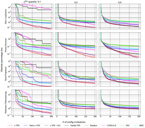
Figure 10: The performance curves on four benchmarks in HPOlib with a constraint of network size. We picked $\gamma_{i}^{\mathrm{true}}=0.1$ (Left), $0.5$ (Center), and $0.9$ (Right). The horizontal axis shows the number of evaluated configurations in optimizations and the vertical axis shows the absolute percentage error in each experiment.

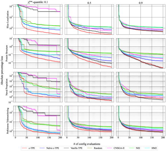
Figure 11: The performance curves on four benchmarks in HPOlib with a constraint of runtime. We picked $\gamma_{i}^{\mathrm{true}}=0.1$ (Left), $0.5$ (Center), and $0.9$ (Right). The horizontal axis shows the number of evaluated configurations in optimizations and the vertical axis shows the absolute percentage error in each experiment.

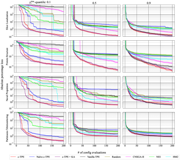
Figure 12: The performance curves on four benchmarks in HPOlib with constraints of runtime and network size. We picked $\gamma_{i}^{\mathrm{true}}=0.1$ (Left), $0.5$ (Center), and $0.9$ (Right). The horizontal axis shows the number of evaluated configurations in optimizations and the vertical axis shows the absolute percentage error in each experiment.

Figure 13: The performance curves on three benchmarks in NAS-Bench-101 with a constraint of network size. We picked $\gamma_{i}^{\mathrm{true}}=0.1$ (Left), $0.5$ (Center), and $0.9$ (Right). The horizontal axis shows the number of evaluated configurations in optimizations and the vertical axis shows the absolute percentage error in each experiment. The scale of the results in $\gamma_{i}^{\mathrm{true}}=0.1$ is different from others, we separately scaled for the readability.

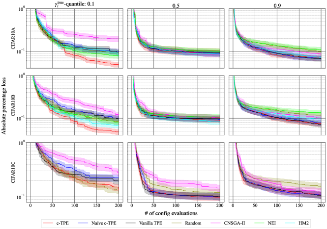
Figure 14: The performance curves on three benchmarks in NAS-Bench-101 with a constraint of runtime. We picked $\gamma_{i}^{\mathrm{true}}=0.1$ (Left), $0.5$ (Center), and $0.9$ (Right). The horizontal axis shows the number of evaluated configurations in optimizations and the vertical axis shows the absolute percentage error in each experiment.

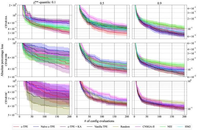
Figure 15: The performance curves on three benchmarks in NAS-Bench-101 with constraints of runtime and network size. We picked $\gamma_{i}^{\mathrm{true}}=0.1$ (Left), $0.5$ (Center), and $0.9$ (Right). The horizontal axis shows the number of evaluated configurations in optimizations and the vertical axis shows the absolute percentage error in each experiment. The scale of the results in $\gamma_{i}^{\mathrm{true}}=0.1$ is different from others, we separately scaled for the readability.

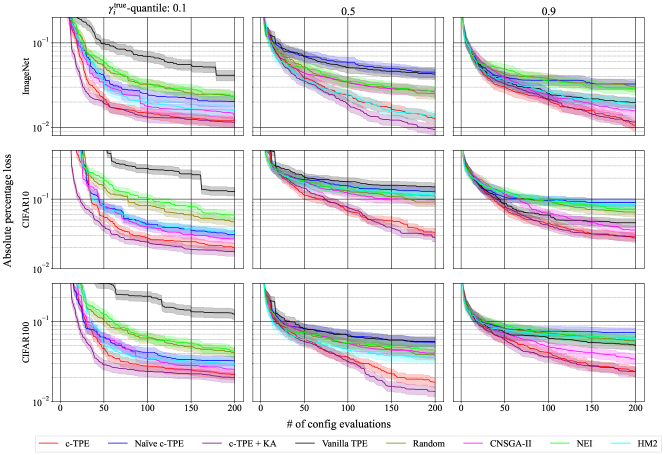
Figure 16: The performance curves on three benchmarks in NAS-Bench-201 with a constraint of network size. We picked $\gamma_{i}^{\mathrm{true}}=0.1$ (Left), $0.5$ (Center), and $0.9$ (Right). The horizontal axis shows the number of evaluated configurations in optimizations and the vertical axis shows the absolute percentage error in each experiment.

Figure 17: The performance curves on three benchmarks in NAS-Bench-201 with a constraint of runtime. We picked $\gamma_{i}^{\mathrm{true}}=0.1$ (Left), $0.5$ (Center), and $0.9$ (Right). The horizontal axis shows the number of evaluated configurations in optimizations and the vertical axis shows the absolute percentage error in each experiment.

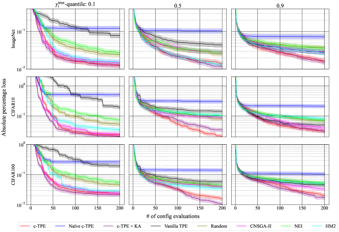
Figure 18: The performance curves on three benchmarks in NAS-Bench-201 with constraints of runtime and network size. We picked $\gamma_{i}^{\mathrm{true}}=0.1$ (Left), $0.5$ (Center), and $0.9$ (Right). The horizontal axis shows the number of evaluated configurations in optimizations and the vertical axis shows the absolute percentage error in each experiment.

Appendix I Additional Results for Section 4.3

Figures 19–21 show the average rank of each method over the number of evaluations. Each figure shows the performance of different constraint settings with 0.1 to 0.9 of $\gamma_{i}^{\mathrm{true}}$.

As the constraint becomes tighter, c-TPE converged quicker in the early stage of the optimizations in all the settings due to KA. On the other hand, KA did not accelerate the optimizations as constraints become looser. This is because it is easy to identify feasible domains in loose constraint settings even by random samplings. However, since KA did not degrade the performance of c-TPE, it is recommended to add KA as much as possible.

Furthermore, it is worth noting that although the performance of HM2 and NEI outperformed the vanilla TPE in tight constraint settings, their performance was degraded as constraints become looser and they did not exhibit better performance than the vanilla TPE with $\gamma_{i}^{\mathrm{true}}=0.9$. On the other hand, c-TPE exhibited better performance than the vanilla TPE even in the settings of $\gamma_{i}^{\mathrm{true}}=0.9$ because it adapted the optimization based on the estimated $\hat{\gamma}_{i}$.

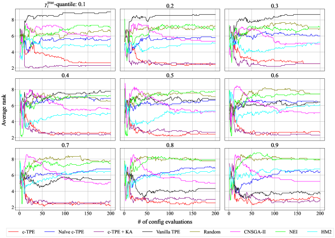
Figure 19: The average rank of each method over the number of evaluations. We evaluated each method on nine benchmarks with the network size constraint and each optimization was repeated over 50 random seeds. Each figure presents the results for $\gamma_{i}^{\mathrm{true}}$ of 0.1 to 0.9, respectively.

Figure 20: The average rank of each method over the number of evaluations. We evaluated each method on nine benchmarks with the runtime constraint and each optimization was repeated over 50 random seeds.

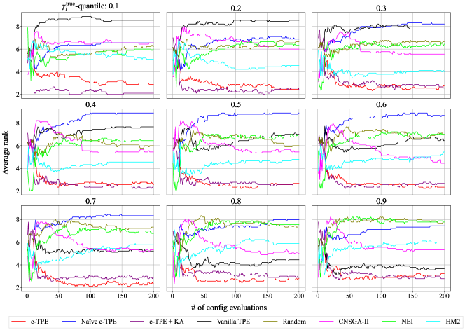
Figure 21: The average rank of each method over the number of evaluations. We evaluated each method on nine benchmarks with the runtime and the network size constraints and each optimization was repeated over 50 random seeds.

bib-style ref

References

- Addison et al. (2022) H. Addison, KS. inversion, H. Ryan, and C. Ted. Happywhale - whale and dolphin identification, 2022.
- Akiba et al. (2019) T. Akiba, S. Sano, T. Yanase, T. Ohta, and M. Koyama. Optuna: A next-generation hyperparameter optimization framework. In International Conference on Knowledge Discovery & Data Mining, 2019.
- Alina et al. (2019) JE. Alina, C. Phil, B. Rodrigo, and G. Victor. Open images 2019 - object detection, 2019.
- Arnold and Hansen (2012) D. Arnold and N. Hansen. A (1+1)-CMA-ES for constrained optimisation. In Genetic and Evolutionary Computation Conference, 2012.
- Awad et al. (2021) N. Awad, N. Mallik, and F. Hutter. DEHB: Evolutionary hyberband for scalable, robust and efficient hyperparameter optimization. arXiv:2105.09821, 2021.
- Bergstra and Bengio (2012) J. Bergstra and Y. Bengio. Random search for hyper-parameter optimization. Journal of Machine Learning Research, 13(2), 2012.
- Bergstra et al. (2011) J. Bergstra, R. Bardenet, Y. Bengio, and B. Kégl. Algorithms for hyper-parameter optimization. In Advances in Neural Information Processing Systems, 2011.
- Bergstra et al. (2013) J. Bergstra, D. Yamins, and D. Cox. Making a science of model search: Hyperparameter optimization in hundreds of dimensions for vision architectures. In International Conference on Machine Learning, 2013.
- Brochu et al. (2010) E. Brochu, V. Cora, and N. de Freitas. A tutorial on Bayesian optimization of expensive cost functions, with application to active user modeling and hierarchical reinforcement learning. arXiv:1012.2599, 2010.
- Chen et al. (2018) Y. Chen, A. Huang, Z. Wang, I. Antonoglou, J. Schrittwieser, D. Silver, and N. de Freitas. Bayesian optimization in alphago. arXiv:1812.06855, 2018.
- Deb et al. (2002) K. Deb, A. Pratap, S. Agarwal, and T. Meyarivan. A fast and elitist multiobjective genetic algorithm: NSGA-II. IEEE Transactions on Evolutionary Computation, 6(2):182–197, 2002.
- Dong and Yang (2020) X. Dong and Y. Yang. NAS-Bench-201: Extending the scope of reproducible neural architecture search. arXiv:2001.00326, 2020.
- Eriksson and Poloczek (2021) D. Eriksson and M. Poloczek. Scalable constrained Bayesian optimization. In International Conference on Artificial Intelligence and Statistics, 2021.
- Falkner et al. (2018) S. Falkner, A. Klein, and F. Hutter. BOHB: Robust and efficient hyperparameter optimization at scale. In International Conference on Machine Learning, 2018.
- Gardner et al. (2014) J. Gardner, M. Kusner, ZE. Xu, K. Weinberger, and J. Cunningham. Bayesian optimization with inequality constraints. In International Conference on Machine Learning, 2014.
- Garnett (2022) R. Garnett. Bayesian Optimization. Cambridge University Press, 2022.
- Garrido-Merchán et al. (2023) EC. Garrido-Merchán, D. Fernández-Sánchez, and D. Hernández-Lobato. Parallel predictive entropy search for multi-objective Bayesian optimization with constraints applied to the tuning of machine learning algorithms. Expert Systems with Applications, 215, 2023.
- Gelbart et al. (2014) M. Gelbart, J. Snoek, and R. Adams. Bayesian optimization with unknown constraints. arXiv:1403.5607, 2014.
- Jones et al. (1998) D. Jones, M. Schonlau, and W. Welch. Efficient global optimization of expensive black-box functions. Journal of Global Optimization, 13(4):455–492, 1998.
- Klein and Hutter (2019) A. Klein and F. Hutter. Tabular benchmarks for joint architecture and hyperparameter optimization. arXiv:1905.04970, 2019.
- Kushner (1964) HJ. Kushner. A new method of locating the maximum point of an arbitrary multipeak curve in the presence of noise. 1964.
- Letham et al. (2019) B. Letham, B. Karrer, G. Ottoni, and E. Bakshy. Constrained Bayesian optimization with noisy experiments. Bayesian Analysis, 14(2):495–519, 2019.
- Liaw et al. (2018) R. Liaw, E. Liang, R. Nishihara, P. Moritz, J. Gonzalez, and I. Stoica. Tune: A research platform for distributed model selection and training. arXiv:1807.05118, 2018.
- Lobato et al. (2015) JH. Lobato, M. Gelbart, M. Hoffman, R. Adams, and Z. Ghahramani. Predictive entropy search for bayesian optimization with unknown constraints. In International Conference on Machine Learning, 2015.
- Loshchilov and Hutter (2016) I. Loshchilov and F. Hutter. CMA-ES for hyperparameter optimization of deep neural networks. arXiv:1604.07269, 2016.
- Loshchilov et al. (2013) I. Loshchilov, M. Schoenauer, and M. Sebag. Bi-population CMA-ES agorithms with surrogate models and line searches. In Genetic and Evolutionary Computation Conference, 2013.
- Melis et al. (2018) G. Melis, C. Dyer, and P. Blunsom. On the state of the art of evaluation in neural language models. In International Conference on Learning Representations, 2018.
- Montes et al. (2006) EM. Montes, J. Velázquez-Reyes, and CA. Coello. Modified differential evolution for constrained optimization. In International Conference on Evolutionary Computation, 2006.
- Nardi et al. (2019) L. Nardi, D. Koeplinger, and K. Olukotun. Practical design space exploration. In International Symposium on Modeling, Analysis, and Simulation of Computer and Telecommunication Systems, pages 347–358. IEEE, 2019.
- Perrone et al. (2019) V. Perrone, I. Shcherbatyi, R. Jenatton, C. Archambeau, and M. Seeger. Constrained Bayesian optimization with max-value entropy search. arXiv:1910.07003, 2019.
- Shahriari et al. (2016) B. Shahriari, K. Swersky, Z. Wang, R. Adams, and N. de Freitas. Taking the human out of the loop: A review of Bayesian optimization. Proceedings of the IEEE, 104(1):148–175, 2016.
- Watanabe (2023) S. Watanabe. Tree-structured Parzen estimator: Understanding its algorithm components and their roles for better empirical performance. arXiv:2304.11127, 2023.
- Ying et al. (2019) C. Ying, A. Klein, E. Christiansen, E. Real, K. Murphy, and F. Hutter. NAS-Bench-101: Towards reproducible neural architecture search. In International Conference on Machine Learning, 2019.