A Comprehensive Study of Radiomics-based Machine Learning for Fibrosis Detection

Abstract

Objectives: Early detection of liver fibrosis can help cure the disease or prevent disease progression. We perform a comprehensive study of machine learning-based fibrosis detection in CT images using radiomic features to develop a non-invasive approach to fibrosis detection.

Methods: Two sets of radiomic features were extracted from spherical ROIs in CT images of 182 patients who underwent simultaneous liver biopsy and CT examinations, one set corresponding to biopsy locations and another distant from biopsy locations. Combinations of contrast, normalization, machine learning model, feature selection method, bin width, and kernel radius were investigated, each of which were trained and evaluated 100 times with randomized development and test cohorts. The best settings were evaluated based on their mean test AUC and the best features were determined based on their frequency among the best settings.

Results: Logistic regression models with NC images normalized using Gamma correction with $\gamma=1.5$ performed best for fibrosis detection. Boruta was the best for radiomic feature selection method. Training a model using these optimal settings and features consisting of first order energy, first order kurtosis, and first order skewness, resulted in a model that achieved mean test AUCs of 0.7549 and 0.7166 on biopsy-based and non-biopsy ROIs respectively, outperforming a baseline and best models found during the initial study.

Conclusions: Logistic regression models trained on radiomic features from NC images normalized using Gamma correction with $\gamma=1.5$ that underwent Boruta feature selection are effective for liver fibrosis detection. Energy, kurtosis, and skewness are particularly effective features for fibrosis detection.

1 Keywords

Machine Learning; Liver; Fibrosis; Humans; Tomography, X-Ray Computed

2 Key points

• We present a comprehensive investigation of settings for machine learning-based liver fibrosis detection in CT images using radiomic features

• We identify the optimal settings for training a machine learning model for liver fibrosis detection using radiomic features, as well as the most prominent radiomic features for fibrosis detection

• We use the derived optimal settings and three radiomic features consisting of energy, kurtosis, and skewness to produce a highly effective model for fibrosis detection

3 Abbreviations and acronyms

• 3D: 3-dimensional

• AUC: Area under the receiver operating characteristic curve

• CE: Contrast-enhanced

• CT: Computed tomography

• DECT: Dual-energy computed tomography

• Gamma-0.5: Gamma correction with $\gamma=0.5$

• Gamma-1.5: Gamma correction with $\gamma=1.5$

• HCC: Hepatocellular carcinoma

• HU: Hounsfield unit

• LASSO: Least absolute shrinkage and selection operator

• ML: Machine learning

• MR: Magnetic resonance

• NAFLD: Nonalcoholic fatty liver disease

• NASH: Nonalcoholic steatohepatitis

• NC: Non-contrast-enhanced

• PCA: Principal component analysis

• RBF: Radial basis function

• ROI: Region of interest

• SAG: Stochastic average gradient

• SAGA: Stochastic average gradient ascent

• SGD: Stochastic gradient descent

• SMOTE: Synthetic minority oversampling technique

• SVM: Support vector machines

• US: Ultrasound

4 Introduction

Diffuse liver diseases such as liver steatosis, fibrosis, and cirrhosis have a high global frequency [1]. More than 30% of adults in developed countries are afflicted with nonalcoholic fatty liver disease (NAFLD) and the overall prevalence of NAFLD worldwide was estimated to be 32.4% [2]. Approximately 30% of patients with NAFLD develop NASH; 30-40% of patients with NASH develop fibrosis and eventually liver cirrohosis, which has a 10-year-mortality of 25%. Hepatocellular carcinoma (HCC) is an inflammation-associated cancer with approximately 90% of HCC burden being associated with prolonged hepatitis due to viral hepatitis, excessive alcohol intake, or NAFLD-NASH [3]. In 2020, HCC was estimated to be the fourth most common overall cause of cancer death globally [4].

The use of computed tomography (CT) imaging for non-invasive detection of diffuse liver disease in patients undergoing CT imaging for extrahepatic clinical indications enables new opportunities for early treatment and cure of such diseases, especially with the introduction of novel therapeutic methods such as obeticholic or aramchol [5, 6] for nonalcoholic steatohepatitis (NASH) [7]. Detecting patients in the pre-cirrhotic phase allows for early application of preventative and corrective measures to combat the progression of the disease, and as a result decrease the mortality rate and the financial burden that comes from the care of complications. Fibrosis is the wound healing response to liver injury and is associated with an increase in liver-related complications in patients with NASH [8]. Thus, screening for liver NASH-fibrosis in general populations [9] is worthwhile because those with early stages of fibrosis are entirely asymptomatic, may have normal transaminase blood levels, and the fibrosis progression is very slow at this point.

Early diagnosis and treatment are paramount as the process leading to end-stage liver disease is reversible when detected in the early stages. Image-guided liver biopsy is the diagnostic reference standard but is costly, can introduce risk of complications to patients, and demonstrates low intra- and interobserver repeatability [10, 11]. Furthermore, due to the diffuse nature of hepatic fibrosis, its accuracy suffers from sampling error ranging between 55% and 75% [12]. These issues have led to interest in developing non-invasive modalities for the detection and evaluation of liver fibrosis [13, 14]. Magnetic resonance (MR) elastography has been the most promising imaging modality thus far for accurate fibrosis staging but requires dedicated equipment. MR imaging access in Canada is limited, and when available is costly and fails to differentiate between stages of fibrosis [15, 16]. Ultrasound (US)-based methods, such as 1-dimensional transient elastography and point shear wave elastography or acoustic radiation force impulse imaging, have reached growing clinical relevance. However, the reported accuracies of the US-based methods have varied significantly with sensitivities ranging from 56-96% depending on the cut-off values for stages of fibrosis using the METAVIR grading system, fibrosis prevalence in the study cohort, and disease etiology [17, 18]. Serum tests are unreliable due to inflammation outside of the liver being able to lead to false-positive results. Bloodtests have demonstrated to be moderately useful for detecting clinically significant fibrosis or cirrhosis in patients with the hepatitis C virus [19].

CT is widely available and often used to image patients with chronic liver diseases. The notable advantage of CT compared to other imaging modalities for fibrosis quantification is the potential to seamlessly incorporate the requirement measurements into multi-phase liver protocols, which can obviate the need for additional dedicated acquisitions, unlike MR and US elastography [20]. Dual-energy CT (DECT) is a new technology shows promise in the fat component from water in unenhanced CT images, and evidence suggests that DECT can be beneficial in non-invasive fibrosis staging within the same diagnostic CT exam [21]. A cause for concern with using CT as opposed to MR imaging and US is that CT uses ionizing radiation, limiting its use as a screen modality in an otherwise healthy population.

Thus it is of great interest to investigate non-invasive approaches to fibrosis detection in CT images. One approach to this problem is by using radiomics features. Cui et al. [22] used the CatBoost regression model [23] to train a machine learning (ML) model to perform detection of significant fibrosis and cirrhosis in precontrast, arterial, portal vein, and multi-phase CT images. Wang et al. [24] used a support vector machine (SVM) [25] to classify significant fibrosis, advanced fibrosis, and cirrhosis from non-contrast, arterial and portal phase CT images. In their work, they used extracted radiomics features selected using least absolute shrinkage and selection operator (LASSO) logistic regression. A similar approach was done by Wang et al. [26] to predict cirrhosis, who used an SVM and LASSO to develop a radiomics signature, which was then used with other clinical predictors to train a logistic regression model.

These works used different approaches to radiomics-based machine learning for fibrosis staging but it is difficult to compare their methods due to factors such as differences in radiomics feature extraction and different target datasets. We aim to perform a robust and effective comparison of different ML approaches to radiomics-based fibrosis detection to help inform how to best approach radiomics-based fibrosis detection using ML. We perform experiments using a plethora of different combinations of settings and compare to determine the best settings for the fibrosis detection task. We also investigate the most prominent features throughout these experiments to inform which features are most clinically relevant for fibrosis detection.

5 Materials and methods

5.1 Data

This study was approved by the University Health Network’s Research Ethics Board (REB) and had informed consent obtained from all involved patients.

The anonymized data used for this study consisted of 3-dimensional (3D) CT scans of livers from 182 patients, with each 3D liver volume having maximal spatial dimensions of 99x512x512 voxels.

When acquiring the CT scans, patients underwent simultaneous random liver biopsy. The biopsy was used to score each patient volume on a 5-point fibrosis score scale based on pathology results which used the METAVIR scoring system. These fibrosis scores were F0: no fibrosis, F1: mild fibrosis, F2: moderate fibrosis, F3: severe fibrosis: F4: cirrhosis. The images were acquired using dual-energy acquisition on an Aquilion ONE Genesis scanner (Canon Medical Systems, Otawara, Japan). The CT scanning used tube voltage of 80 kV and 135 kV, 0.5 mm slice thickness, 0.5 second gantry revolving time, and 320x0.5 mm detector collimation. The field of view was adjusted according to each patient’s body habitus. Images were reconstructed using iterative reconstruction AIDR-3D using a 512x512 pixel matrix, and 120 kVp equivalent images were generated by blending the 80 kVp and 135 kVp images together. Each liver volume was resampled to $0.5\times 0.5\times 0.5$ mm to standardize the voxel sizes between volumes.

Two types of volumes were available; non-contrast-enhanced (NC) and contrast-enhanced (CE). However, some patients only had one volume available. 8 patients in the dataset only had NC volumes and 1 patient in the dataset only had a CE volume. Furthermore, 13 NC volumes and 12 CE volumes had ambiguous or uncertain fibrosis stages and were thus excluded, resulting with 168 NC volumes and 162 CE volumes.

The attenuation values of the liver volumes ranged from -1024 Hounsfield unit (HU) to 4096 HU but the liver tissue only is only visualized by a small subset of this range of values. To reduce the impact of irrelevant information, enhance contrast, and prevent normalization methods from reducing the relevant voxels to insignificant attenuation values, the attenuation values for NC volumes were thresholded to a range of 0 HU to 100 HU and the attenuation values for CE volumes were thresholded to a range of -10 HU to 200 HU, as was done by [27]. These thresholding values were recommended by a board certified radiologist with 31 years of clinical experience.

To perform fibrosis detection, we simplified the ground truth labels to no fibrosis and fibrosis by assigning each patient volume a ground truth label of 0 if they had a fibrosis stage of F0 and 1 if they had a fibrosis stage of F1-F4.

5.2 Regions of Interest

Spherical regions of interest (ROI) of 1.5 cm radius were placed such that their center was 2.5 cm distal to the biopsy needle to ensure that the chosen ROIs were consistent with the corresponding biopsy. An example is presented in Figure 1. This was to ensure that the initial set of ROIs captured a region with a fibrosis stage consistent with that recorded by the biopsy. This is due to the diffuse nature of fibrosis, as the fibrosis stage in a given region of a liver can differ by $\pm$ 1 fibrosis stage.

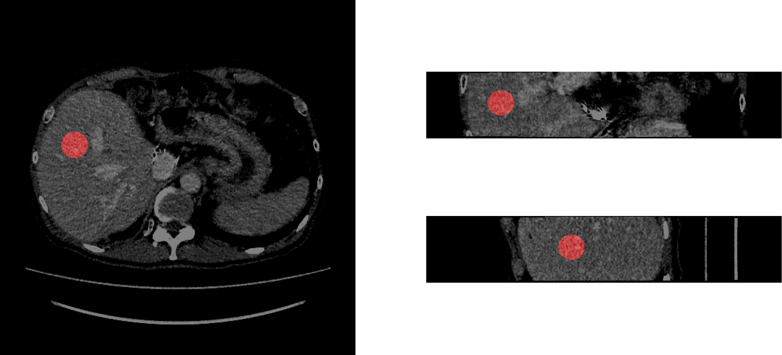
Figure 1: Example ROI (left: axial view, upper right: coronal view, lower right: sagittal view).

Some initial placements for the ROIs were such that they were not fully enclosed within the liver. To resolve this issue, the flawed ROIs were shifted such that they were fully encapsulated within the ROI. Each shift was a maximum of 3 cm along any axis. An example of a flawed ROI and the post-shift ROI is presented in Figure 2.

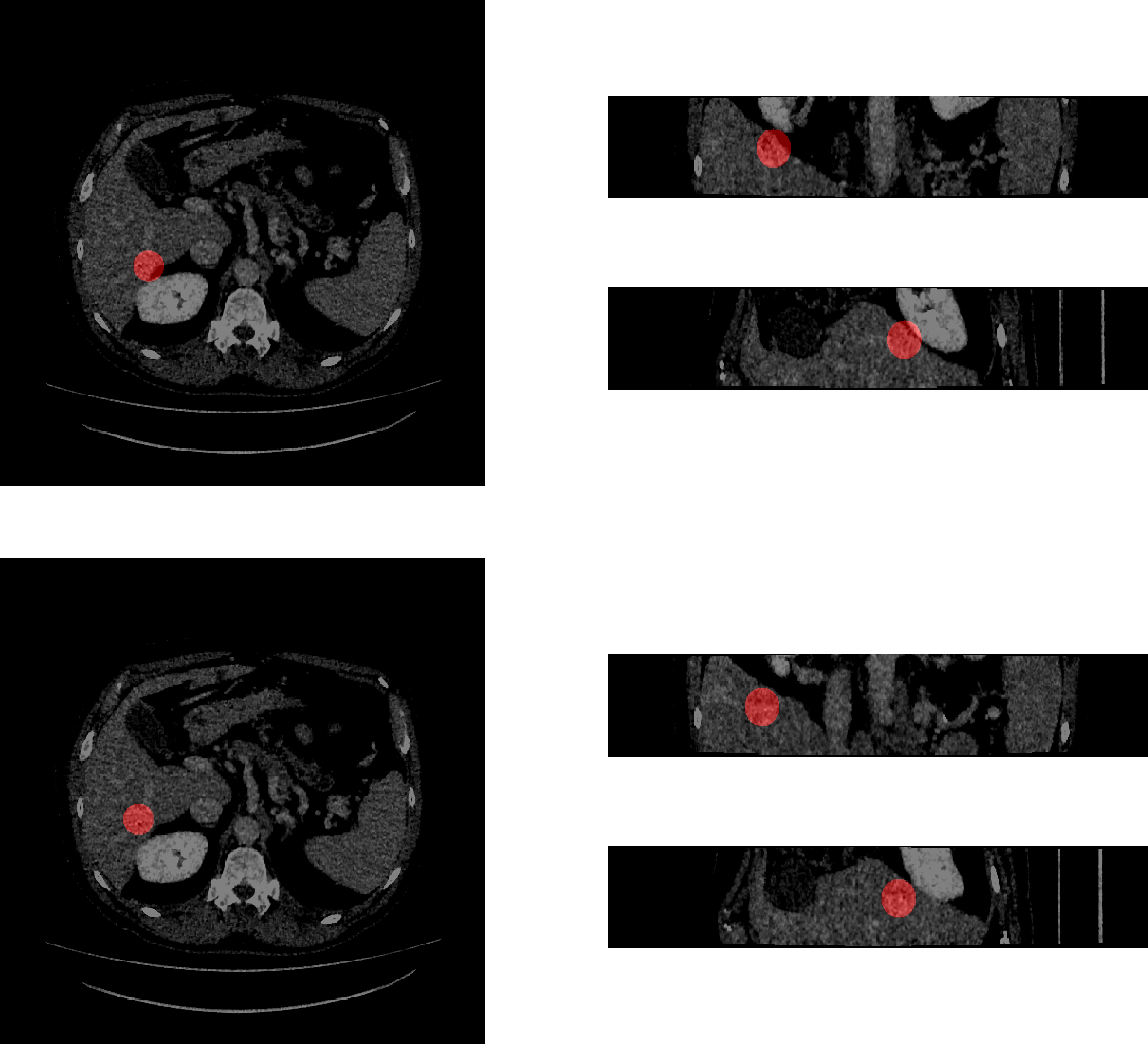
Figure 2: Example flawed ROI (above) and the ROI post-shift (below) (left: axial view, upper right: coronal view, lower right: sagittal view).

To evaluate the ability for the radiomics models to predict fibrosis stages in liver regions outside of the biopsy-based ROIs, we assigned an additional ROI for each NC and CE volume. The ROIs distal to the biopsy needle will be referred to as biopsy-based ROIs and these new ROIs will be referred to as non-biopsy ROIs. The assignment of these ROIs were semi-random, with preference towards the left liver lobe. The centers of the non-biopsy ROIs were at minimum 3 cm away from the centers of the biopsy-based ROIs. All ROIs were visually confirmed by a licensed radiologist.

5.3 Radiomics Extraction

We used the PyRadiomics, an open source Python library, to perform the radiomics feature extraction [28]. 1725 radiomics features were extracted from each ROI. The diagnostic features and shape features were removed as diagnostic features do not contain useful information for fibrosis classification and shape features are dependent on the original pixel spacing of the volume and other factors such as the choice of ROI which may not generalize to other studies.

5.4 Settings

To perform our comparative study, we considered different possible values for a range of settings and performed experiments for every possible combination of settings, totalling 1728 different configurations. These settings and their candidate values are presented in Table 1.

Table 1: Settings and their candidate values.

Setting	Candidate Values
Contrast	NC
	CE
Normalization method	None
	Histogram equalization
	Min-max
	Z-score
	Gamma-0.5
	Gamma-1.5
Machine learning model type	Logistic regression classifier
	Random forest classifier [29]
	Support vector machines (SVM) [25]
	Linear models with stochastic gradient descent (SGD) training
Feature selection method	None
	Principal component analysis (PCA)
	Boruta
	LASSO regression
Bin Width	15
	25
	35
Kernel Radius	1
	2
	3

Different normalization methods for the liver volumes were also explored. With histogram normalization, each volume was contrast adjusted based on their histogram of values using the scikit-image Python library [30]. Min-max normalization was used to scale each liver volume between 0 and 1. Z-score normalization scales each liver volume to a mean of 0 and a standard deviation of 1. Gamma-0.5 and Gamma-1.5 refers to Gamma correction, with $\gamma=0.5$ and Gamma correction with $\gamma=1.5$ respectively. For a given image X, applying Gamma correction results with $X^{\gamma}$.

Bin width and kernel radius are settings specific to PyRadiomics, detailed in Section 5.3. Bin width specifies the size of each bin used during gray value discretization. The default value for the bin width in PyRadiomics is 25. The kernel radius refers to the size of the neighborhood around each voxel to consider when computing feature maps. A greater kernel radius indicates that a greater area around each voxel is considered [28]. The default value for the kernel radius in PyRadiomics is 1.

5.5 Experimentation Design

Inspired by Liu et al. [31], 100 experiments were run for each permutation of settings detailed in Section 5.4. For each experiment, the data was randomly split into a development set and a test set using 80/20 splits. Once split into the development and test cohorts, The cohorts were individually processed. First, redundant features that had a correlation greater than 0.95 with another feature were removed. Then features with variance less than 0.05 were removed as they do not discriminate between different cases. Finally, the features in each cohort were min-max scaled to range [0, 1].

During each of the 100 experiments, the development set was further split into two sub-cohorts using 75/25 splits, referred to as grid-search train and grid-search validation respectively. These sub-cohorts, were used to perform a grid search of ML model specific hyperparameters. The data splits are visualized in Figure 3.

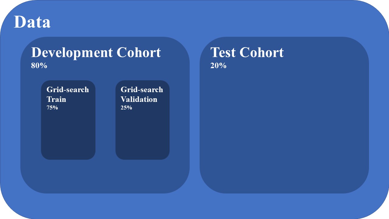
Figure 3: Visualized data cohort splits.

The number of positive and negative samples available for each permutation of relevant settings are summarized in Table 2. There is a consistent class imbalance where negative classes are more prevalent than positive classes. The Synthetic Minority Oversampling Technique (SMOTE) algorithm [32] was used to address this class imbalance. The SMOTE algorithm was applied to data used to train a model prior to the training.

Table 2: Number of positive and negative classes for NC and CE.

Class	NC	CE
Positive	$64$	$62$
Negative	$104$	$100$

The grid search of ML model specific hyperparameters was done by training ML models using each combination of model specific hyperparameters 30 times using the grid-search train cohort and evaluating the area under the receiver operating characteristic curve (AUC) on the grid-search validation cohort across the 30 runs. The combination of model specific hyperparameters that resulted with the greatest mean AUC was used as the model’s hyperparameters for the current combination of settings. These ML model specific hyperparameters, which differ from the settings listed in Section 5.4, are based on their implementations in the scikit-learn Python library and are presented in Table 3.

Table 3: Model type-specific hyperparameters and their candidate values.

Model Type	Hyperparameter	Candidate Values
Logistic Regression	Optimization Solver	L-BFGS-B
		Newton-CG
		LIBLINEAR
		Stochastic Average Gradient (SAG)
		Stochastic Average Gradient Ascent (SAGA) [33]
	Inverse Regularization Strength	0.5
		1.0
		1.5
Random Forest	Number of Estimators	50
		100
		200
	Maximum number of features calculation method	50
		Auto
		Square Root
SVM	Kernel	Linear
		Polynomial (degree 3)
		Radial Basis Function (RBF)
	Inverse L2 Squared Regularization Strength	0.5
		1.0
		1.5
Linear Model with SGD	L2 Regularization Strength	0.001
		0.0001
		0.00001
	Loss Function	Logistic Regression
		Modified Huber Loss

Once the model specific hyperparameters were chosen, they were used in conjunction with the current combination of settings to train the model using the development cohort and was subsequently evaluated on the test cohort of patient volumes. The model was evaluated on both the features from the biopsy-based ROIs and the features from the non-biopsy ROIs of the test cohort, forming two sets of test results. The features from the non-biopsy ROIs are only used at this point. This process was repeated with each of the 100 experiments for each configuration of settings having random cohorts. This experiment design is visualized in Figure 4.

Figure 4: Visualized experiment design.

6 Results

The mean biopsy-based test AUC and mean non-biopsy test AUC for the considered settings are presented in Table 4. For this table, the best result for each setting is in bold. The mean biopsy-based test AUC across all experiments is 0.6501 and the mean non-biopsy test AUC across all experiments is 0.6078.

Table 4: Average test performance for each bin width and kernel radius value.

Setting	Value	Biopsy-based ROIs		Non-biopsy ROIs
		Test AUC	CI	Test AUC	CI
Contrast	NC	0.6809	[0.6646, 0.6972]	0.6499	[0.6326, 0.6671]
	CE	0.6194	[0.6018, 0.6371]	0.5658	[0.5473, 0.5843]
Normalization	None	0.6372	[0.6203, 0.6541]	0.6326	[0.6147, 0.6505]
	Histogram Equalization	0.6525	[0.6345, 0.6704]	0.5686	[0.5502, 0.5870]
	Min-Max	0.6537	[0.6369, 0.6705]	0.6167	[0.5989, 0.6345]
	Z-Score	0.6346	[0.6176, 0.6515]	0.6025	[0.5849, 0.6202]
	Gamma-0.5	0.6383	[0.6215, 0.6550]	0.6094	[0.5919, 0.6268]
	Gamma-1.5	0.6847	[0.6683, 0.7011]	0.6172	[0.5992, 0.6352]
Model	Logistic Regression	0.6661	[0.6495, 0.6828]	6242	[0.6069, 0.6415]
	Random Forest	0.6385	[0.6218, 0.6552]	0.6007	[0.5827, 0.6186]
	SVM	0.6429	[0.6301, 0.6645]	0.6040	[0.5860, 0.6221]
	Linear with SGD	0.6487	[0.6315, 0.666]	0.6024	[0.5842, 0.6207]
Feature Selection	None	0.6425	[0.6257, 0.6593]	0.6017	[0.5840, 0.6193]
	PCA	0.6345	[0.6172, 0.6518]	0.5906	[0.5721, 0.6090]
	Boruta	0.6723	[0.6555, 0.6892]	0.6372	[0.6195, 0.6548]
	Lasso Regression	0.6513	[0.6344, 0.6682]	0.6020	[0.5842, 0.6197]
	15	0.6492	[0.6322, 0.6661]	0.6077	[0.5900, 0.6254]
Bin Width	25	0.6502	[0.6332, 0.6672]	0.6087	[0.5908, 0.6265]
	35	0.6511	[0.6341, 0.6680]	0.6071	[0.5891, 0.6251]
	1	0.6502	[0.6332, 0.6671]	0.6078	[0.5899, 0.6257]
Kernel Radius	2	0.6500	[0.6331, 0.6670]	0.6078	[0.5900, 0.6257]
	3	0.6503	[0.6333, 0.6672]	0.6079	[0.5900, 0.6258]

It can be seen that the mean test AUC does not vary significantly as the bin width or the kernel radius change. Thus it can be concluded that the impact of these settings are insignificant. The other settings excluding normalization had a single value that performed best on both biopsy-based and non-biopsy ROIs. These settings were NC for contrast, logistic regression for the model, and Boruta for the feature selection. Gamma correction with $\gamma=1.5$ performed best for test while no normalization performed best using the non-biopsy ROIs.

The five best combinations of settings using biopsy-based ROIs and their corresponding mean AUC on the grid-search validation and test cohorts are presented in Table 5.

Table 5: Settings and AUC scores for the five best setting combinations evaluated on test cohorts of biopsy-based ROIs.

Settings						Test Performance
Normalization	Feature Selection	Model	Contrast	Bin Width	Kernel Radius	AUC	CI
Gamma-1.5	Boruta	Logistic Regression	NC	25	2	0.7497	[0.7346, 0.7648]
Gamma-1.5	Boruta	Logistic Regression	NC	15	1	0.7496	[0.7336, 0.7655]
Gamma-1.5	Boruta	SGD	NC	35	3	0.7486	[0.7339, 0.7633]
Gamma-1.5	Boruta	SGD	NC	15	2	0.7485	[0.7335, 0.7635]
Gamma-1.5	Boruta	Logistic Regression	NC	15	2	0.7481	[0.7330, 0.7632]

These results demonstrate that Gamma-1.5 normalization, Boruta feature selection, and NC are the best settings for this task. Logistic regression also proves to be the best model but linear models with SGD demonstrated the potential to be effective for fibrosis detection when combined with the other settings.

The five best combinations of settings using non-biopsy ROIs and their corresponding mean AUC on the grid-search validation and test cohorts are presented in Table 6.

Table 6: Settings and AUC scores for the five best setting combinations evaluated on test cohorts of non-biopsy ROIs.

Settings						Test Performance
Normalization	Feature Selection	Model	Contrast	Bin Width	Kernel Radius	AUC	CI
Gamma-1.5	Boruta	Random Forest	NC	15	1	0.7128	[0.6948, 0.7307]
Gamma-1.5	Boruta	Random Forest	NC	25	3	0.7098	[0.6937, 0.7259]
None	Boruta	Logistic Regression	NC	15	1	0.7088	[0.6938, 0.7238]
None	Boruta	Logistic Regression	NC	25	1	0.7088	[0.6955, 0.7220]
None	Boruta	Logistic Regression	NC	15	3	0.7086	[0.6936, 0.7236]

Boruta and NC proved to continue being the best feature selection and contrast, respectively. However, despite logistic regression and no normalization having the highest mean AUC using non-biopsy ROIs across all experiments, the two best configurations used random forest models and Gamma-1.5 normalization. This indicates that the two best configurations for random test work best with these specific combination of settings.

6.1 Feature Rankings

An overall ranking of the importance of features across all trained models were calculated for both the test results using biopsy-based ROIs and the test results using non-biopsy ROIs by first filtering the top 5 features from each experiment and then counting the total number of occurrences of each filtered feature across all models. It should be noted that some experiments had less than 5 non-negligible features, in which case all features were accounted for. The top 12 features across all models on biopsy-based ROIs can be found in Figure 5 and the top 12 features across all models on non-biopsy ROIs can be found in Figure 6.

Figure 5: Top 12 features across all experiments using biopsy-based ROIs.

Figure 6: Top 12 features across all experiments using non-biopsy ROIs.

The most notable aspect of these features is the overlap in most common features between the models trained using the biopsy-based ROIs and the non-biopsy ROIs. The only top features across all experiments to not overlap are wavelet_HLH_glszm_ZoneEntropy from the models trained using biopsy-based ROIs and wavelet_LHL_glszm_HighAreaHighGrayLevelEmphasis from the models trained using the non-biopsy ROIs.

The top 12 features were also calculated across the 5 best models using both sets of ROIs. These results can be found in Figure 7 and Figure 8 respectively.

Figure 7: Top 12 features across the 5 best model configurations using biopsy-based ROIs.

Figure 8: Top 12 features across the 5 best model configurations using non-biopsy ROIs.

The top features curated from the top 5 models trained using each set of ROIs differ significantly from the top features across all experiments. However, they are similar in that features involving maximum, energy, kurtosis, and skewness remain present. There is a significant discrepancy between the frequency of the top 5 features compared to the remaining 7 features in Figure 7, indicating that these are the most important features when training using the biopsy-based models. Between these 5 features, only three features are present in the top features for the best model configurations trained using non-biopsy ROIs. These features are original_firstorder_Energy, original_firstorder_Kurtosis, and original_firstorder_Skewness. original_firstorder_Energy is the most prominent as it is significantly more common than any other feature across the experiments involving the 5 best model configurations using non-biopsy ROIs. The importance of first order energy is consistent with the findings of Cui et al. [22] in their work in fibrosis staging using multi-phase CT images. Based on these results we theorize that these three features are the most important for radiomics-based fibrosis detection among the features provided by PyRadiomics.

6.2 Model Performance Using the Three Most Important Features

Based on the findings from Section 6.1 that original_firstorder_Energy, original_firstorder_Kurtosis, and original_firstorder_Skewness are the most important features for fibrosis detection, we trained a logistic regression model on NC images normalized using Gamma-1.5 normalization without using feature selection and using all permutations of bin width and kernel radius. We chose these settings as they were the best performing settings. We did not use any feature selection as we are only using three features and we used all permutations of bin width and kernel radius as we found the differences in AUC between different values of bin width and kernel radius to be insignificant. This model configuration using the three features will be referred to as the parsimonious model. We found that across all experiments performed using these settings, the parsimonious models achieved a mean AUC of 0.7549 on biopsy-based ROIs and a mean AUC of 0.7166 on non-biopsy ROIs. These results surpass the best mean test AUCs on both sets of ROIs presented in Table 5 and Table 6. A comparison between the parsimonious models, the 5 models that performed best on the biopsy-based test ROIs, and the 5 models that performed best on the non-biopsy test ROIs is presented in Table 7. A comparison of sensitivity values and specificity values are presented in Table 8. It should be noted that due to the settings and feature selection being informed by the dataset, the results of this model are likely overfit to the dataset. As such, these results serve to demonstrate the potential performance and effectiveness of these settings and features in the context of fibrosis detection.

Table 7: Mean Test AUC of Parsimonious Model Compared to Five Best Models Based on their Test Performance on each Set of ROIs.

Model	Biopsy-based ROIs		Non-biopsy ROIs
	Test AUC	CI	Test AUC	CI
Parsimonious Model	0.7549	[0.7399, 0.7699]	0.7166	[0.7017, 0.7315]
Best Model on Biopsy-based Test ROIs	0.7497	[0.7346, 0.7648]	0.7015	[0.6863, 0.7167]
2nd Best Model on Biopsy-based Test ROIs	0.7496	[0.7336, 0.7655]	0.7042	[0.6878, 0.7205]
3rd Best Model on Biopsy-based Test ROIs	0.7486	[0.7339, 0.7633]	0.7043	[0.6881, 0.7205]
4th Best Model on Biopsy-based Test ROIs	0.7485	[0.7335, 0.7635]	0.7027	[0.6870, 0.7183]
5th Best Model on Biopsy-based Test ROIs	0.7481	[0.7330, 0.7632]	0.7056	[0.6894, 0.7218]
Best Model on Non-biopsy Test ROIs	0.7131	[0.6986, 0.7276]	0.7128	[0.6948, 0.7307]
2nd Best Model on Non-biopsy Test ROIs	0.7070	[0.6920, 0.7220]	0.7098	[0.6937, 0.7259]
3rd Best Model on Non-biopsy Test ROIs	0.7208	[0.7056, 0.7360]	0.7088	[0.6938, 0.7238]
4th Best Model on Non-biopsy Test ROIs	0.7181	[0.7044, 0.7317]	0.7088	[0.6955, 0.7220]
5th Best Model on Non-biopsy Test ROIs	0.7168	[0.7026, 0.7310]	0.7086	[0.6936, 0.7236]

Table 8: Sensitivity and Specificity of Parsimonious Model Compared to Five Best Models Based on their Test Performance on each Set of ROIs.

Model	Biopsy-based ROIs		Non-biopsy ROIs
	Sensitivity	Specificity	Sensitivity	Specificity
Parsimonious Model	0.8100	0.5995	0.8297	0.5338
Best Model on Biopsy-based Test ROIs	0.7565	0.5986	0.7660	0.5445
2nd Best Model on Biopsy-based Test ROIs	0.7600	0.5991	0.7761	0.5509
3rd Best Model on Biopsy-based Test ROIs	0.7215	0.6170	0.7448	0.5588
4th Best Model on Biopsy-based Test ROIs	0.7307	0.6124	0.7469	0.5489
5th Best Model on Biopsy-based Test ROIs	0.7637	0.5962	0.7644	0.5477
Best Model on Non-biopsy Test ROIs	0.6404	0.6438	0.6677	0.6356
2nd Best Model on Non-biopsy Test ROIs	0.6258	0.6472	0.6525	0.6325
3rd Best Model on Non-biopsy Test ROIs	0.7964	0.5372	0.8209	0.4745
4th Best Model on Non-biopsy Test ROIs	0.7349	0.5733	0.7767	0.5391
5th Best Model on Non-biopsy Test ROIs	0.7387	0.5642	0.7871	0.5320

6.3 Comparison to Baseline

A baseline method to compare to was also implemented based on the work by Hirano et al. [34]. The selected baseline method was a combination of a combination of the following 3 features:

• 2D wavelet decomposition feature

• Standard deviation of variance filter

• Mean CT intensity

The three features were passed to a logistic regression model with L2 regularization. The most notable difference between the methodology applied for the baseline’s original work and the version implemented for this work was the ROI selection. The baseline’s original work used 5 manually selected cubic ROIs whereas this work used 1 spherical ROI. The baseline acquired an AUC of 0.86 in its original work.

Table 9 presents the AUC achieved by the baseline compared to the results of the parsimonious model presented in Section 6.2, and Table 10 compares the sensitivity and specificity values. Although the baseline model showed comparable performance, it was outperformed by the parsimonious model in AUC, sensitivity, and specificity on both sets of ROIs.

Table 9: Mean Test AUC of Parsimonious Model Compared to Baseline Model.

Model	Biopsy-based ROIs		Non-biopsy ROIs
	Test AUC	CI	Test AUC	CI
Parsimonious Models	0.7549	[0.7399, 0.7699]	0.7166	[0.7017, 0.7315]
Baseline Model	0.7425	[0.7278, 0.7572]	0.7126	[0.6973, 0.7280]

Table 10: Sensitivity and Specificity of Parsimonious Model Compared to Baseline Model.

Model	Biopsy-based ROIs		Non-biopsy ROIs
	Sensitivity	Specificity	Sensitivity	Specificity
Parsimonious Models	0.8100	0.5995	0.8297	0.5338
Baseline Model	0.7827	0.5971	0.7878	0.5581

6.4 Robustness to ROI Volume Confoundment

Welch et al. [35] found that features from PyRadiomics that are dependent on image attenuation such as energy can effectively serve as surrogates for delineated tumour volume, even when shape features such as volume are not meant to be considered. To ensure that the findings of this work are independent of the ROI volume, a model was trained using the MeshVolume feature, the primary volume metric for PyRadiomics, and another model was trained using the pixel spacing values of each image. Both models were trained using NC images normalized using Gamma-1.5 normalization, and no feature selection, as was done for the parsimonious model in Section 6.2. All permutations of bin width and kernel radius were used. The models trained using MeshVolume were trained using a logistic regression model while the model trained using pixel spacing values were trained using logistic regression models and random forest models. The pixel spacing serves as an effective measure of ROI volume as all ROIs are spheres with 1.5 cm radii. Thus, the differences between the volumes of ROIs between images can be measured using the pixel spacing as they impact how many voxels constitute the ROI.

The performance of these models are presented in Table 11. These results indicate that while there is some volume information, there is significant additional signal present beyond volume in the models trained using PyRadiomics features in this work. Thus, the volume information is ultimately not a strong confounding factor in the presented results.

Table 11: Mean Test AUC of Volume Dependent Models.

Model	Biopsy-based ROIs		Non-biopsy ROIs
	Test AUC	CI	Test AUC	CI
Mesh Volume Models	0.5053	[0.5231, 0.5641]	0.4857	[0.5231, 0.5641]
Pixel Spacing Models	0.5437	[0.4875, 0.5230]	0.5437	[0.4684, 0.5029]

7 Discussion

Our study of ML-based fibrosis detection using radiomics features demonstrated valuable insights into effective fibrosis detection such as NC images normalized using Gamma correction with $\gamma=1.5$ being the overall most effective approach for fibrosis detection. This indicates that despite CE images being easier for humans to identify fibrosis in, the CE images obfuscate information valuable for fibrosis detection that are present in NC images, this information being further emphasized by Gamma correction. We also demonstrated that logistic regression classifiers are effective models for the fibrosis detection task and when using a plethora of radiomic features, Boruta is the ideal feature selection approach. We found that the choice of bin width and kernel radius are negligibly relevant for fibrosis detection. We also presented the most prominent radiomic features for fibrosis detection and proposed that first order energy, first order kurtosis, and first order skewness are the most useful features for fibrosis detection among the evaluated radiomic features. We trained a parsimonious logistic regression classifier using these three features to produce a highly effective classifier for fibrosis detection.

Our parsimonious radiomics model not only outperformed the best performing radiomic models trained using all radiomic features prior to feature selection, but also outperformed an effective baseline model proposed by Hirano et al. [34]. The performance of our parsimonious model and the baseline model demonstrate that in the context of fibrosis detection, reducing available features to a select few critical and clinically relevant features may be more effective than using a large subset of the available features. Our parsimonious model also indicates the value and effectiveness of energy, kurtosis, and skewness for fibrosis detection, which we encourage future work to use as a starting point for developing fibrosis detection models.

One notable limitation of our study is the selection of ROIs. We used ROIs distal to the biopsy needle due to concern that designating ROIs significantly distant from the biopsy needle would result with an ROI that captured an area with a different fibrosis stage than the fibrosis stage specified from biopsy. Relying on ROIs based on biopsy needles are not ideal for non-invasive fibrosis detection and the fibrosis detection would ideally not require any specific ROI. The baseline results also imply that the ROI selection is important for fibrosis detection. Hirano et al. [34] achieved significantly higher AUC values in their work with the major difference in their implementation and our implementation of their baseline being the ROI selection. Non-invasive solutions to fibrosis detection in CT images would ideally not be reliant on ROI selection. Another limitation with this work is that while it was found that Gamma correction with $\gamma=1.5$ outperformed Gamma correction with $\gamma=0.5$, higher $\gamma$ values were not explored. It is possible that higher values could further improve classification performance.

8 Conclusion

We present an in-depth investigation of settings for radiomics-based fibrosis detection and find that NC images normalized using Gamma correction with $\gamma=1.5$ classified using logistic regression classifier models perform best on average for fibrosis detection. We also demonstrate that when using numerous radiomic features, Boruta feature selection is best for reducing the number of features. We find that first order energy, first order kurtosis, and first order skewness are particularly effective features for fibrosis detection and demonstrate that a model that solely uses these three features can be effective for fibrosis detection. The findings of this work can serve as a starting point and bolster future research into fibrosis detection.

References

- Monelli et al. [2021] Filippo Monelli, Giulia Besutti, Olivera Djuric, et al. The effect of diffuse liver diseases on the occurrence of liver metastases in cancer patients: A systematic review and meta-analysis. Cancers, 13(9):2246, May 2021. ISSN 2072-6694. doi: 10.3390/cancers13092246. URL https://www.mdpi.com/2072-6694/13/9/2246.
- Riazi et al. [2022] Kiarash Riazi, Hassan Azhari, Jacob H Charette, et al. The prevalence and incidence of nafld worldwide: a systematic review and meta-analysis. The Lancet Gastroenterology & Hepatology, 7(9):851–861, Sep 2022. ISSN 24681253. doi: 10.1016/S2468-1253(22)00165-0. URL https://linkinghub.elsevier.com/retrieve/pii/S2468125322001650.
- Llovet et al. [2016] Josep M. Llovet, Jessica Zucman-Rossi, Eli Pikarsky, et al. Hepatocellular carcinoma. Nature Reviews Disease Primers, 2(1):16018, Dec 2016. ISSN 2056-676X. doi: 10.1038/nrdp.2016.18. URL http://www.nature.com/articles/nrdp201618.
- can [2020] Cancer today, 2020. URL https://gco.iarc.fr/today/online-analysis-pie?v=2020&mode=cancer&mode_population=continents&population=900&populations=900&key=total&sex=0&cancer=39&type=1&statistic=5&prevalence=0&population_group=0&ages_group%5B%5D=0&ages_group%5B%5D=17&nb_items=7&group_cancer=1&include_nmsc=1&include_nmsc_other=1&half_pie=0&donut=0.
- Ratziu et al. [2021] V. Ratziu, L. de Guevara, R. Safadi, et al. Aramchol in patients with nonalcoholic steatohepatitis: a randomized, double-blind, placebo-controlled phase 2b trial. Nature Medicine, 27(10):1825–1835, Oct 2021. ISSN 1078-8956, 1546-170X. doi: 10.1038/s41591-021-01495-3. URL https://www.nature.com/articles/s41591-021-01495-3.
- Llovet et al. [2021] Josep M. Llovet, Robin Kate Kelley, Augusto Villanueva, et al. Hepatocellular carcinoma. Nature Reviews Disease Primers, 7(1):6, Dec 2021. ISSN 2056-676X. doi: 10.1038/s41572-020-00240-3. URL http://www.nature.com/articles/s41572-020-00240-3.
- Schuster and Feldstein [2017] Susanne Schuster and Ariel E. Feldstein. Novel therapeutic strategies targeting ask1 in nash. Nature Reviews Gastroenterology & Hepatology, 14(6):329–330, Jun 2017. ISSN 1759-5045, 1759-5053. doi: 10.1038/nrgastro.2017.42. URL http://www.nature.com/articles/nrgastro.2017.42.
- Dulai et al. [2017] Parambir S. Dulai, Siddharth Singh, Janki Patel, et al. Increased risk of mortality by fibrosis stage in nonalcoholic fatty liver disease: Systematic review and meta-analysis: Dulai et al. Hepatology, 65(5):1557–1565, May 2017. ISSN 02709139. doi: 10.1002/hep.29085. URL https://onlinelibrary.wiley.com/doi/10.1002/hep.29085.
- García-Compeán et al. [2020] Diego García-Compeán, Jesús Zacarías Villarreal-Pérez, Manuel Enrique de la O. Cavazos, et al. Prevalence of liver fibrosis in an unselected general population with high prevalence of obesity and diabetes mellitus. time for screening? Annals of Hepatology, 19(3):258–264, May 2020. ISSN 16652681. doi: 10.1016/j.aohep.2020.01.003. URL https://linkinghub.elsevier.com/retrieve/pii/S1665268120300077.
- Kose et al. [2015] Sukran Kose, Gursel Ersan, Bengu Tatar, et al. Evaluation of percutaneous liver biopsy complications in patients with chronic viral hepatitis. The Eurasian Journal of Medicine, 47(3):161–164, Nov 2015. ISSN 13088734, 13088742. doi: 10.5152/eurasianjmed.2015.107. URL https://www.eajm.org//en/evaluation-of-percutaneous-liver-biopsy-complications-in-patients-with-chronic-viral-hepatitis-132814.
- Rockey et al. [2009] Don C. Rockey, Stephen H. Caldwell, Zachary D. Goodman, et al. Liver biopsy. Hepatology, 49(3):1017–1044, Mar 2009. ISSN 02709139. doi: 10.1002/hep.22742. URL https://onlinelibrary.wiley.com/doi/10.1002/hep.22742.
- Bedossa et al. [2003] Pierre Bedossa, Delphine Dargere, and Valerie Paradis. Sampling variability of liver fibrosis in chronic hepatitis c. Hepatology, 38(6):1449–1457, Dec 2003. ISSN 02709139. doi: 10.1016/j.hep.2003.09.022. URL http://doi.wiley.com/10.1016/j.hep.2003.09.022.
- Nallagangula et al. [2018] Krishna Sumanth Nallagangula, Shashidhar Kurpad Nagaraj, Lakshmaiah Venkataswamy, and Muninarayana Chandrappa. Liver fibrosis: a compilation on the biomarkers status and their significance during disease progression. Future Science OA, 4(1):FSO250, Jan 2018. ISSN 2056-5623. doi: 10.4155/fsoa-2017-0083. URL https://www.future-science.com/doi/10.4155/fsoa-2017-0083.
- non [2015] Journal of Hepatology, 63(1):237–264, Jul 2015. ISSN 01688278. doi: 10.1016/j.jhep.2015.04.006. URL https://linkinghub.elsevier.com/retrieve/pii/S0168827815002597.
- Ragazzo et al. [2017] Taisa Grotta Ragazzo, Denise Paranagua-Vezozzo, Fabiana Roberto Lima, et al. Accuracy of transient elastography-fibroscan®, acoustic radiation force impulse (arfi) imaging, the enhanced liver fibrosis (elf) test, apri, and the fib-4 index compared with liver biopsy in patients with chronic hepatitis c. Clinics, 72(9):516–525, 2017. ISSN 18075932. doi: 10.6061/clinics/2017(09)01. URL https://linkinghub.elsevier.com/retrieve/pii/S1807593222011905.
- Singh et al. [2015] Siddharth Singh, Sudhakar K. Venkatesh, Zhen Wang, et al. Diagnostic performance of magnetic resonance elastography in staging liver fibrosis: A systematic review and meta-analysis of individual participant data. Clinical Gastroenterology and Hepatology, 13(3):440–451.e6, Mar 2015. ISSN 15423565. doi: 10.1016/j.cgh.2014.09.046. URL https://linkinghub.elsevier.com/retrieve/pii/S1542356514013950.
- Sigrist et al. [2017] Rosa M.S. Sigrist, Joy Liau, Ahmed El Kaffas, et al. Ultrasound elastography: Review of techniques and clinical applications. Theranostics, 7(5):1303–1329, 2017. ISSN 1838-7640. doi: 10.7150/thno.18650. URL http://www.thno.org/v07p1303.htm.
- Newsome et al. [2020] Philip N Newsome, Magali Sasso, Jonathan J Deeks, et al. Fibroscan-ast (fast) score for the non-invasive identification of patients with non-alcoholic steatohepatitis with significant activity and fibrosis: a prospective derivation and global validation study. The Lancet Gastroenterology & Hepatology, 5(4):362–373, Apr 2020. ISSN 24681253. doi: 10.1016/S2468-1253(19)30383-8. URL https://linkinghub.elsevier.com/retrieve/pii/S2468125319303838.
- Chou and Wasson [2013] Roger Chou and Ngoc Wasson. Blood tests to diagnose fibrosis or cirrhosis in patients with chronic hepatitis c virus infection: A systematic review. Annals of Internal Medicine, 158(11):807, Jun 2013. ISSN 0003-4819. doi: 10.7326/0003-4819-158-11-201306040-00005. URL http://annals.org/article.aspx?doi=10.7326/0003-4819-158-11-201306040-00005.
- Sofue et al. [2018] Keitaro Sofue, Masakatsu Tsurusaki, Achille Mileto, et al. Dual-energy computed tomography for non-invasive staging of liver fibrosis: Accuracy of iodine density measurements from contrast-enhanced data: Staging of liver fibrosis in dual-energy ct. Hepatology Research, 48(12):1008–1019, Nov 2018. ISSN 13866346. doi: 10.1111/hepr.13205. URL https://onlinelibrary.wiley.com/doi/10.1111/hepr.13205.
- Lamb et al. [2015] Peter Lamb, Dushyant V. Sahani, Jorge M. Fuentes-Orrego, et al. Stratification of patients with liver fibrosis using dual-energy ct. IEEE Transactions on Medical Imaging, 34(3):807–815, Mar 2015. ISSN 0278-0062, 1558-254X. doi: 10.1109/TMI.2014.2353044. URL https://ieeexplore.ieee.org/document/6887313.
- Cui et al. [2021] Enming Cui, Wansheng Long, Juanhua Wu, et al. Predicting the stages of liver fibrosis with multiphase ct radiomics based on volumetric features. Abdominal Radiology, 46(8):3866–3876, Aug 2021. ISSN 2366-004X, 2366-0058. doi: 10.1007/s00261-021-03051-6. URL https://link.springer.com/10.1007/s00261-021-03051-6.
- Dorogush et al. [2018] Anna Veronika Dorogush, Vasily Ershov, and Andrey Gulin. Catboost: gradient boosting with categorical features support, 2018. URL https://arxiv.org/abs/1810.11363.
- Wang et al. [2022] Jincheng Wang, Shengnan Tang, Yingfan Mao, et al. Radiomics analysis of contrast-enhanced ct for staging liver fibrosis: an update for image biomarker. Hepatology International, 16(3):627–639, Jun 2022. ISSN 1936-0541. doi: 10.1007/s12072-022-10326-7.
- Platt [2000] John Platt. Probabilistic outputs for support vector machines and comparisons to regularized likelihood methods. Adv. Large Margin Classif., 10, 06 2000.
- Wang et al. [2020] Jin-Cheng Wang, Rao Fu, Xue-Wen Tao, et al. A radiomics-based model on non-contrast ct for predicting cirrhosis: make the most of image data. Biomarker Research, 8:47, 2020. ISSN 2050-7771. doi: 10.1186/s40364-020-00219-y.
- Yin et al. [2021] Yunchao Yin, Derya Yakar, Rudi A. J. O. Dierckx, et al. Liver fibrosis staging by deep learning: a visual-based explanation of diagnostic decisions of the model. European Radiology, 31(12):9620–9627, Dec 2021. ISSN 0938-7994, 1432-1084. doi: 10.1007/s00330-021-08046-x. URL https://link.springer.com/10.1007/s00330-021-08046-x.
- van Griethuysen et al. [2017] Joost J.M. van Griethuysen, Andriy Fedorov, Chintan Parmar, et al. Computational radiomics system to decode the radiographic phenotype. Cancer Research, 77(21):e104–e107, Nov 2017. ISSN 0008-5472, 1538-7445. doi: 10.1158/0008-5472.CAN-17-0339. URL https://aacrjournals.org/cancerres/article/77/21/e104/662617/Computational-Radiomics-System-to-Decode-the.
- Breiman [2001] Leo Breiman. Random forests. Machine Learning, 45(1):5–32, 2001. ISSN 08856125. doi: 10.1023/A:1010933404324. URL http://link.springer.com/10.1023/A:1010933404324.
- van der Walt et al. [2014] Stéfan van der Walt, Johannes L. Schönberger, Juan Nunez-Iglesias, et al. scikit-image: image processing in python. PeerJ, 2:e453, Jun 2014. ISSN 2167-8359. doi: 10.7717/peerj.453. URL https://peerj.com/articles/453.
- Liu et al. [2021] Xiaoyang Liu, Farzad Khalvati, Khashayar Namdar, et al. Can machine learning radiomics provide pre-operative differentiation of combined hepatocellular cholangiocarcinoma from hepatocellular carcinoma and cholangiocarcinoma to inform optimal treatment planning? European Radiology, 31(1):244–255, Jan 2021. ISSN 0938-7994, 1432-1084. doi: 10.1007/s00330-020-07119-7. URL https://link.springer.com/10.1007/s00330-020-07119-7.
- Blagus and Lusa [2013] Rok Blagus and Lara Lusa. Smote for high-dimensional class-imbalanced data. BMC Bioinformatics, 14(1):106, Dec 2013. ISSN 1471-2105. doi: 10.1186/1471-2105-14-106. URL https://bmcbioinformatics.biomedcentral.com/articles/10.1186/1471-2105-14-106.
- Defazio et al. [2014] Aaron Defazio, Francis Bach, and Simon Lacoste-Julien. Saga: A fast incremental gradient method with support for non-strongly convex composite objectives. In Z. Ghahramani, M. Welling, C. Cortes, et al., editors, Advances in Neural Information Processing Systems, volume 27. Curran Associates, Inc., 2014. URL https://proceedings.neurips.cc/paper/2014/file/ede7e2b6d13a41ddf9f4bdef84fdc737-Paper.pdf.
- Hirano et al. [2022] Ryo Hirano, Patrik Rogalla, Christin Farrell, et al. Development of a classification method for mild liver fibrosis using non-contrast ct image. International Journal of Computer Assisted Radiology and Surgery, 17(11):2041–2049, Aug 2022. ISSN 1861-6429. doi: 10.1007/s11548-022-02724-x. URL https://link.springer.com/10.1007/s11548-022-02724-x.
- Welch et al. [2019] Mattea L. Welch, Chris McIntosh, Benjamin Haibe-Kains, et al. Vulnerabilities of radiomic signature development: The need for safeguards. Radiotherapy and Oncology, 130:2–9, 2019. ISSN 0167-8140. doi: https://doi.org/10.1016/j.radonc.2018.10.027. URL https://www.sciencedirect.com/science/article/pii/S0167814018335515.