Link Prediction with Non-Contrastive
Learning

Abstract

Graph neural networks (GNNs) are prominent in the graph machine learning domain, owing to their strong performance across various tasks. A recent focal area is the space of graph self-supervised learning (SSL), which aims to derive useful node representations without labeled data. Notably, many state-of-the-art graph SSL approaches are contrastive methods, which use a combination of positive and negative samples to learn node representations. Owing to challenges in negative sampling (slowness and model sensitivity), recent literature introduced non-contrastive methods, which instead only use positive samples. Though such methods have shown promising performance in node-level tasks, their suitability for link prediction tasks, which are concerned with predicting link existence between pairs of nodes, and have broad applicability to recommendation systems contexts, is yet unexplored. In this work, we extensively evaluate the performance of existing non-contrastive methods for link prediction in both transductive and inductive settings. While most existing non-contrastive methods perform poorly overall, we find that, surprisingly, BGRL generally performs well in transductive settings. However, it performs poorly in the more realistic inductive settings where the model has to generalize to links to/from unseen nodes. We find that non-contrastive models tend to overfit to the training graph and use this analysis to propose T-BGRL, a novel non-contrastive framework that incorporates cheap corruptions to improve the generalization ability of the model. This simple modification strongly improves inductive performance in 5/6 of our datasets, with up to a 120% improvement in Hits@50—all with comparable speed to other non-contrastive baselines, and up to 14× faster than the best-performing contrastive baseline. Our work imparts interesting findings about non-contrastive learning for link prediction and paves the way for future researchers to further expand upon this area.

1 Introduction

Graph neural networks (GNNs) are ubiquitously used modeling tools for relational graph data, with widespread applications in chemistry (Chen et al., 2019; Guo et al., 2021; 2022a; Liu et al., 2022), forecasting and traffic prediction (Derrow-Pinion et al., 2021; Tang et al., 2020), recommendation systems (Ying et al., 2018b; He et al., 2020; Sankar et al., 2021; Tang et al., 2022; Fan et al., 2022), graph generation (You et al., 2018; Fan & Huang, 2019; Shiao & Papalexakis, 2021), and more. Given significant challenges in obtaining labeled data, one particularly exciting recent direction is the advent of graph self-supervised learning (SSL), which aims to learn representations useful for various downstream tasks without using explicit supervision besides available graph structure and node features (Zhu et al., 2020; Jin et al., 2021; Thakoor et al., 2022; Bielak et al., 2022).

One prominent class of graph SSL approaches are contrastive methods (Jin et al., 2020). These methods typically utilize contrastive losses such as InfoNCE (Oord et al., 2018) or margin-based losses (Ying et al., 2018b) between node and negative sample representations. However, such methods usually require either many negative samples (Hassani & Ahmadi, 2020) or carefully chosen ones (Ying et al., 2018b; Yang et al., 2020), where the first one results with quadratic number of in-batch comparisons, and the latter is especially expensive on graphs since we often store the sparse adjacency matrix instead of its dense complement (Thakoor et al., 2022; Bielak et al., 2022). These drawbacks motivated the development of non-contrastive methods (Thakoor et al., 2022; Bielak et al., 2022; Zhang et al., 2021; Kefato & Girdzijauskas, 2021), based on advances in the image domain (Grill et al., 2020; Chen & He, 2021; Chen et al., 2020), which do not require negative samples and solely rely on augmentations. This allows for a large speedup compared to their contrastive counterparts with strong performance (Bielak et al., 2022; Zhang et al., 2021).

However, non-contrastive SSL methods are typically evaluated on node-level tasks, which is a more direct analog of image classification in the graph domain. In comparison, the link-level task (link prediction), which focuses on predicting link existence between pairs of nodes, is largely overlooked. This presents a critical gap in understanding: Are non-contrastive methods suitable for link prediction tasks? When do they (not) work, and why? This gap presents a huge opportunity, since link prediction is a cornerstone in the recommendation systems community (He et al., 2020; Zhang & Chen, 2019; Berg et al., 2017).

Present Work. To this end, our work first performs an extensive evaluation of non-contrastive SSL methods in link prediction contexts to discover the impact of different augmentations, architectures, and non-contrastive losses. We evaluate all of the (to the best of our knowledge) currently existing non-contrastive methods: CCA-SSG (Zhang et al., 2021), Graph Barlow Twins (GBT) (Bielak et al., 2022), and Bootstrapped Graph Latents (BGRL) (Thakoor et al., 2022) (which has the same design as the independently proposed SelfGNN (Kefato & Girdzijauskas, 2021)). We also compare these methods against a baseline end-to-end GCN (Kipf & Welling, 2017) with cross-entropy loss, and two contrastive baselines: GRACE (Zhu et al., 2020), and a GCN trained with max-margin loss (Ying et al., 2018a). We evaluate the methods in the transductive setting and find that BGRL (Thakoor et al., 2022) greatly outperforms not only the other non-contrastive methods, but also GRACE—a strong augmentation-based contrastive model for node classification. Surprisingly, BGRL even performs on-par with a margin-loss GCN (with the exception of 2/6 datasets). However, in the more realistic inductive setting, which considers prediction between new edges and nodes at inference time, we observe a huge gap in performance between BGRL and a margin-loss GCN (ML-GCN). Upon investigation, we find that BGRL is unable to sufficiently push apart the representations of negative links from positive links when new nodes are introduced, owing to a form of overfitting. To address this, we propose T-BGRL, a novel non-contrastive method which uses a corruption function to generate cheap “negative” samples—without performing the expensive negative sampling step of contrastive methods. We show that it greatly reduces overfitting tendencies, and outperforms existing non-contrastive methods across 5/6 datasets on the inductive setting. We also show that it maintains comparable speed with BGRL, and is 14× faster than the margin-loss GCN on the Coauthor-Physics dataset.

Main Contributions. In short, our main contributions are as follows:

• To the best of our knowledge, this is the first work to explore link prediction with non-contrastive SSL methods.

• We show that, perhaps surprisingly, BGRL (an existing non-contrastive model) works well in the transductive link prediction, with performance at par with contrastive baselines, implicitly behaving similarly to other contrastive models in pushing apart positive and negative node pairs.

• We show that non-contrastive SSL models underperform their contrastive counterparts in the inductive setting, and notice that they generalize poorly due to a lack of negative examples.

• Equipped with this understanding, we propose T-BGRL, a novel non-contrastive method that uses cheap “negative” samples to improve generalization. T-BGRL is simple to implement, very efficient when compared to contrastive methods, and improves on BGRL’s inductive performance in 5/6 datasets, making it at or above par with the best contrastive baselines.

2 Preliminaries

Notation. We denote a graph as $G=({\mathcal{V}},{\mathcal{E}})$, where ${\mathcal{V}}$ is the set of $n$ nodes (i.e., $n=|{\mathcal{V}}|$) and ${\mathcal{E}}\subseteq{\mathcal{V}}\times{\mathcal{V}}$ be the set of edges. Let the node-wise feature matrix be denoted by ${\bm{X}}\in\mathbb{R}^{n\times f}$, where $f$ is the number of raw features, and its $i$-th row ${\bm{x}}_{i}$ is the feature vector for the $i$-th node. Let ${\bm{A}}\in\{0,1\}^{n\times n}$ denote the binary adjacency matrix. We denote the graph’s learned node representations as ${\bm{H}}\in\mathbb{R}^{n\times d}$, where $d$ is the size of latent dimension, and ${\bm{h}}_{i}$ is the representation for the $i$-th node. Let ${\bm{Y}}\in\{0,1\}^{n\times n}$ be the desired output for link prediction, as ${\mathcal{E}}$ and ${\bm{A}}$ may have validation and test edges masked off. Similarly, let $\hat{{\bm{Y}}}\in\{0,1\}^{n\times n}$ be the output predicted by the decoder for link prediction. Let Orc be a perfect oracle function for our link prediction task, i.e., $\textsc{Orc}{}({\bm{A}},{\bm{X}})={\bm{Y}}$. Let $\textsc{Neigh}(u)=\{v\ |\ (u,v)\in{\mathcal{E}}\lor(v,u)\in{\mathcal{E}}\}$. Note that we use the terms “embedding” and “representation” interchangeably in this work.

GNNs for Link Prediction. Many new approaches have also been developed with the recent advent of graph neural networks (GNNs). A predominant paradigm is the use of node-embedding-based methods (Hamilton et al., 2017; Berg et al., 2017; Ying et al., 2018b; Zhao et al., 2022b). Node-embedding-based methods typically consist of an encoder ${\bm{H}}=\textsc{Enc}({\bm{A}},{\bm{X}})$ and a decoder $\textsc{Dec}({\bm{H}})$. The encoder model is typically a message-passing based Graph Neural Network (GNN) (Kipf & Welling, 2017; Hamilton et al., 2017; Zhang et al., 2020). The message-passing iterations of a GNN for a node $u$ can be described as follows:

$${\bm{h}}_{u}^{(k+1)}=\textsc{Update}^{(k)}\left({\bm{h}}_{u}^{(k)},\textsc{Aggregate}^{(k)}(\{{\bm{h}}_{v}^{(k)},\forall v\in\textsc{Neigh}(u)\})\right)$$ (1)

where Update and Aggregate are differentiable functions, and ${\bm{h}}^{(0)}_{u}={\bm{x}}_{u}$. The decoder model is usually an inner product or MLP applied on a concatenation of Hadamard product of the source and target learned node representations (Rendle et al., 2020; Wang et al., 2021).

Graph SSL. Below, we define a few terms used throughout our work which helps set the context for our discussion.

Definition 2.1 (Augmentation).

An augmentation $\textsc{Aug}^{+}{}$ is a label-preserving random transformation function $\textsc{Aug}^{+}{}:({\bm{A}},{\bm{X}}){\rightarrow}(\tilde{{\bm{A}}},\tilde{{\bm{X}}})$ that does not change the oracle’s expected value: $\mathbb{E}{[\textsc{Orc}{}(\textsc{Aug}^{+}({\bm{A}},{\bm{X}}))]}={\bm{Y}}$.

Definition 2.2 (Corruption).

A corruption $\textsc{Aug}^{-}{}$ is a label-altering random transformation $\textsc{Aug}^{-}{}:({\bm{A}},{\bm{X}})\rightarrow(\check{{\bm{A}}},\check{{\bm{X}}})$ that changes the oracle’s expected value: $\mathbb{E}{[\textsc{Orc}{}(\textsc{Aug}^{-}({\bm{A}},{\bm{X}}))]}\neq{\bm{Y}}$.

Definition 2.3 (Contrastive Learning).

Contrastive methods select anchor samples (e.g. nodes) and then compare those samples to both positive samples (e.g. neighbors) and negative samples (e.g. non-neighbors) relative to those anchor samples.

Definition 2.4 (Non-Contrastive Learning).

Non-contrastive methods select anchor samples, but only compare those samples to variants of themselves, without leveraging other samples in the dataset.

BGRL. While we examine the performance of all of the non-contrastive graph models, we focus our detailed analysis exclusively on BGRL (Thakoor et al., 2022) due to its superior performance in link prediction when compared to GBT (Bielak et al., 2022) and CCA-SSG (Zhang et al., 2021). BGRL consists of two encoders, one of which is referred to as the online encoder $\textsc{Enc}_{\theta}$; the other is referred to as the target encoder $\textsc{Enc}_{\phi}$. BGRL also incorporates a predictor Pred (typically a MLP) and two sets of augmentations: ${\mathcal{A}}^{+}_{1},{\mathcal{A}}^{+}_{2}$. A single training step for BGRL is as follows: (a) we apply these augmentations: $(\tilde{{\bm{A}}}^{(1)},\tilde{{\bm{X}}}^{(1)})=\textsc{Aug}^{+}_{1}({\bm{A}},{\bm{X}});\ (\tilde{{\bm{A}}}^{(2)},\tilde{{\bm{X}}}^{(2)})=\textsc{Aug}^{+}_{2}({\bm{A}},{\bm{X}})$. (b) we perform forward propagation ${\bm{H}}=\textsc{Enc}(\tilde{{\bm{A}}}^{(1)},\tilde{{\bm{X}}}^{(1)});{\bm{H}}_{2}=\textsc{Enc}(\tilde{{\bm{A}}}^{(2)},\tilde{{\bm{X}}}^{(2)})$. (c) we pass the output through the predictor ${\bm{Z}}=\textsc{Pred}({\bm{H}}_{1})$. (d) we use the mean pairwise cosine distance of ${\bm{Z}}$ and ${\bm{H}}_{2}$ as the loss (see Eqn. 2). (e) $\textsc{Enc}_{\theta}$ is updated via backpropagation and $\textsc{Enc}_{\phi}$ is updated via exponential moving average (EMA) from $\textsc{Enc}_{\theta}$. The BGRL loss is as follows:

$${\mathcal{L}}_{\mathrm{BGRL}}=-\frac{2}{n}\sum^{n-1}_{i=0}\frac{\tilde{{\bm{z}}}_{i}\cdot{\bm{h}}_{i}^{(2)}}{||\tilde{{\bm{z}}}_{i}||\ ||{\bm{h}}_{i}^{(2)}||}$$ (2)

In the next section, we evaluate BGRL and other non-contrastive link prediction methods against contrastive baselines.

3 Do Non-Contrastive Learning Methods Perform Well on Link Prediction Tasks?

Several non-contrastive methods have been proposed and have shown effectiveness in node classification (Kefato & Girdzijauskas, 2021; Thakoor et al., 2022; Zhang et al., 2021; Bielak et al., 2022). However, none of these methods evaluate or target link prediction tasks. We thus aim to answer the following questions: First, how well do these methods work for link prediction compared to existing contrastive/end-to-end baselines? Second, do they work equally well in both transductive and inductive settings? Finally, if they do work, why; if not, why not?

Differences from Node Classification. Link prediction differs from node classification in several key aspects. First, we must consider the embedding of both the source and destination nodes. Second, we have a much larger set of candidates for the same graph—$O(n^{2})$ instead of $O(n)$. Finally, in real applications, link prediction is usually treated as a ranking problem, where we want positive links to be ranked higher than negative links, rather than as a classification problem, e.g. in recommendation systems, where we want to retrieve the top-$k$ most likely links (Cremonesi et al., 2010; Hubert et al., 2022). We discuss this in more detail in Section 3.1 below. Given these differences, it is unclear if methods performing well on node classification naturally perform well on link prediction tasks.

Ideal Link Prediction. What does it mean to perform well on link prediction? We clarify this point here. For some nodes $u,v,w\in{\mathcal{V}}$, let $(u,v)\in{\mathcal{E}}$ and $(u,w)\not\in{\mathcal{E}}$. Then, an ideal encoder for link prediction would have $\textsc{Dist}({\bm{h}}_{u},{\bm{h}}_{v})<\textsc{Dist}({\bm{h}}_{u},{\bm{h}}_{w})$ for some distance function Dist. This idea is the core motivation behind margin-loss-based models (Ying et al., 2018a; Hamilton et al., 2017).

3.1 Evaluation

Datasets. We use datasets from three different domains: citation networks, co-authorship networks, and co-purchase networks. We use the Cora and Citeseer citation networks (Sen et al., 2008), the Coauthor-CS and Coauthor-Physics co-authorship networks, and the Amazon-Computers and Amazon-Photos co-purchase networks (Shchur et al., 2018). We include dataset statistics in Section A.1.

Metric. Following work in the heterogeneous information network (Chen et al., 2018), knowledge-graph (Lin et al., 2015), and recommendation systems (Cremonesi et al., 2010; Hubert et al., 2022) communities, we choose to use Hits@$k$ over AUC-ROC metrics, since we often empirically prioritize ranking candidate links from a selected node context (e.g. ranking the probability that user $A$ will buy item $B$, $C$, or $D$), as opposed to arbitrarily ranking a randomly chosen positive over negative link (e.g. ranking whether the probability that user $A$ buys item $B$ is more likely than user $C$ does not buy item $D$). We report Hits@50 ($k=50$) to strike a balance between the smaller datasets like Cora and the larger datasets like Coauthor-Physics. However, for completeness of the evaluation, we also include AUC-ROC results in Section A.8.

Decoder. Since our goal is to evaluate the performance of the encoder, we use the same decoder for all of our experiments across all of the methods. The choice of decoder has also been previously studied (Wang et al., 2021; 2022), so we use the best-performing decoder - a Hadamard product MLP. For a candidate link $(u,v)$, we have $\hat{{\bm{Y}}}=\textsc{Dec}({\bm{h}}_{u}*{\bm{h}}_{v})$ where $*$ represents the Hadamard product, and Dec is a two-layer MLP (with 256 hidden units) followed by a sigmoid. For the self-supervised methods, we first train the encoder and freeze its weights before training the decoder. As a contextual baseline, we also report results on an end-to-end GCN (E2E-GCN), for which we train the encoder and decoder jointly, backpropagating a binary cross-entropy loss on link existence.

Table 1: Transductive performance of different link prediction methods. We bold the best-performing method and underline the second-best method for each dataset. BGRL consistently outperforms other non-contrastive methods and GRACE, and also outperforms ML-GCN, on 3/6 datasets.

	End-To-End	Contrastive		Non-Contrastive
Dataset	E2E-GCN	ML-GCN	GRACE	CCA-SSG	GBT	BGRL
Cora	0.816$\pm$0.013	0.815$\pm$0.002	0.686$\pm$0.056	0.348$\pm$0.091	0.460$\pm$0.149	0.792$\pm$0.015
Citeseer	0.822$\pm$0.017	0.771$\pm$0.020	0.707$\pm$0.068	0.249$\pm$0.168	0.472$\pm$0.196	0.858$\pm$0.020
Amazon-Photos	0.642$\pm$0.029	0.430$\pm$0.032	0.486$\pm$0.025	0.369$\pm$0.013	0.434$\pm$0.038	0.562$\pm$0.013
Amazon-Computers	0.426$\pm$0.036	0.320$\pm$0.060	0.240$\pm$0.027	0.201$\pm$0.032	0.258$\pm$0.008	0.346$\pm$0.018
Coauthor-CS	0.762$\pm$0.010	0.787$\pm$0.011	0.456$\pm$0.066	0.229$\pm$0.018	0.298$\pm$0.033	0.515$\pm$0.016
Coauthor-Physics	0.798$\pm$0.018	0.810$\pm$0.003	OOM	0.157$\pm$0.009	0.187$\pm$0.011	0.476$\pm$0.015

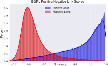
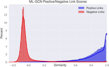
Figure 1: These plots show similarities between node embeddings. Left: distribution of positive/negative link similarities for BGRL. Right: distribution of positive/negative link similarities for ML-GCN. We can see that while they behave similarly, the ML-GCN does a better job of ensuring that positive/negative links are well separated. These scores are computed on Amazon-Photos.

3.1.1 Transductive Evaluation

Transductive Setting. We first evaluate the performance of the methods in the transductive setting, where we train on $G_{train}=({\mathcal{V}},{\mathcal{E}}_{train})$ for ${\mathcal{E}}_{train}\subset{\mathcal{E}}$, validate our method on $G_{val}=({\mathcal{V}},{\mathcal{E}}_{val})$ for ${\mathcal{E}}_{val}\subset({\mathcal{E}}-{\mathcal{E}}_{train})$, and test on $G_{test}=({\mathcal{V}},{\mathcal{E}}_{test})$ for ${\mathcal{E}}_{test}={\mathcal{E}}-{\mathcal{E}}_{train}-{\mathcal{E}}_{val}$. Note that the same nodes are present in training, validation, and testing. We also do not introduce any new edges during inference time—inference is performed on ${\mathcal{E}}_{train}$.

Results. The results of our evaluation are shown in Table 1. As expected, the end-to-end GCN generally performs the best across all of the datasets. We also find that CCA-SSG and GBT similarly perform poorly relative to the other methods. This is intuitive, as neither method was designed for link prediction and were only evaluated for node classification in their respective papers. Surprisingly, however, BGRL outperforms the ML-GCN (the strongest contrastive baseline) on 3/6 of the datasets and performs similarly on 1 other (Cora). It also outperforms GRACE across all of the datasets.

Understanding BGRL Performance. Interestingly, we find that BGRL exhibits similar behavior to the ML-GCN on many datasets, despite the BGRL loss function (see Equation 2) not explicitly optimizing for this. Relative to an anchor node $u$, we can express the max-margin loss of the ML-GCN as follows:

$$L(u)=\mathbb{E}_{v\sim\textsc{Neigh}(u)}\left[\mathbb{E}_{w\sim{\mathcal{E}}-\textsc{Neigh}(u)}J(u,v,w)\right]$$ (3)

where $J(u,v,w)$ is the margin ranking loss for an anchor $u$, positive sample $v$, and negative $w$:

$$J(u,v,w)=\max\{0,{\bm{h}}_{u}\cdot{\bm{h}}_{v}-{\bm{h}}_{u}\cdot{\bm{h}}_{w}+\Delta\}$$ (4)

and $\Delta$ is a hyperparameter for the size of the margin. This seemingly explicitly optimizes for the aforementioned ideal link prediction behavior (anchor-aware ranking of positive over negative links). Despite these circumstances, Figure 1 shows that both BGRL and ML-GCN both clearly separate positive and negative samples, although ML-GCN pushes them further apart. We provide some intuition on why this may occur in Section A.10 below.

Why Does BGRL Not Collapse? The loss function for BGRL (see Equation 2) is 0 when $h_{i}^{(2)}$ = 0 or $\tilde{{\bm{z}}}_{i}$ = 0, i.e., the loss is minimized when the model produces all-zero outputs. While theoretically possible, this is clearly undesirable behavior since this does not result in useful embeddings. We refer to this case as model collapse. It is not fully understood why non-contrastive models do not collapse, but there have been several reasons proposed in the image domain with both theoretical and empirical grounding. We discuss this more in Section A.9. Consistent with the findings from Thakoor et al. (2022), we find that collapse does not occur in practice (with reasonable hyperparameter selection).

Conclusion. We find that CCA-SSG and GBT generally perform poorly compared to contrastive baselines. Surprisingly, we find that BGRL generally performs well in the transductive setting by successfully separating positive and negative link distance distributions. However, this setting may not be representative of real-world problems. In the next section, we evaluate the methods in the more realistic inductive setting to see if this performance holds.

Table 2: Performance of various methods in the inductive setting. See Section 3.1.2 for an explanation of our inductive setting. Although we do not introduce T-BGRL until Section 4, we include the results here to save space.

	End-To-End	Contrastive		Non-Contrastive
Dataset	E2E-GCN	ML-GCN	GRACE	GBT	CCA-SSG	BGRL	T-BGRL
Overall
Cora	0.523$\pm$0.019	0.490$\pm$0.028	0.448$\pm$0.043	0.135$\pm$0.077	0.120$\pm$0.018	0.324$\pm$0.184	0.568$\pm$0.033
Citeseer	0.621$\pm$0.034	0.661$\pm$0.036	0.514$\pm$0.053	0.305$\pm$0.026	0.170$\pm$0.071	0.526$\pm$0.055	0.727$\pm$0.027
Coauthor-Cs	0.484$\pm$0.048	0.572$\pm$0.037	0.313$\pm$0.017	0.182$\pm$0.025	0.176$\pm$0.013	0.438$\pm$0.025	0.534$\pm$0.026
Coauthor-Physics	0.386$\pm$0.016	0.550$\pm$0.059	OOM	0.112$\pm$0.014	0.037$\pm$0.051	0.439$\pm$0.013	0.463$\pm$0.023
Amazon-Computers	0.179$\pm$0.010	0.279$\pm$0.044	0.212$\pm$0.057	0.172$\pm$0.015	0.155$\pm$0.013	0.270$\pm$0.034	0.312$\pm$0.027
Amazon-Photos	0.420$\pm$0.123	0.478$\pm$0.008	0.262$\pm$0.010	0.289$\pm$0.032	0.182$\pm$0.072	0.460$\pm$0.023	0.450$\pm$0.017
Performance on Observed-Observed Node Edges
Cora	0.574$\pm$0.020	0.490$\pm$0.029	0.557$\pm$0.038	0.149$\pm$0.084	0.124$\pm$0.026	0.345$\pm$0.196	0.624$\pm$0.027
Citeseer	0.610$\pm$0.023	0.621$\pm$0.021	0.602$\pm$0.050	0.358$\pm$0.031	0.197$\pm$0.082	0.605$\pm$0.045	0.768$\pm$0.021
Coauthor-Cs	0.504$\pm$0.047	0.591$\pm$0.034	0.332$\pm$0.018	0.187$\pm$0.023	0.177$\pm$0.013	0.462$\pm$0.025	0.535$\pm$0.026
Coauthor-Physics	0.390$\pm$0.015	0.566$\pm$0.058	OOM	0.117$\pm$0.014	0.039$\pm$0.054	0.445$\pm$0.012	0.469$\pm$0.023
Amazon-Computers	0.177$\pm$0.009	0.278$\pm$0.044	0.212$\pm$0.059	0.169$\pm$0.016	0.155$\pm$0.014	0.270$\pm$0.034	0.313$\pm$0.027
Amazon-Photos	0.418$\pm$0.123	0.483$\pm$0.009	0.265$\pm$0.011	0.295$\pm$0.031	0.185$\pm$0.070	0.467$\pm$0.023	0.457$\pm$0.015
Performance on Observed-Unobserved Node Edges
Cora	0.462$\pm$0.023	0.487$\pm$0.021	0.367$\pm$0.045	0.128$\pm$0.075	0.115$\pm$0.014	0.309$\pm$0.175	0.528$\pm$0.037
Citeseer	0.645$\pm$0.055	0.705$\pm$0.039	0.458$\pm$0.063	0.280$\pm$0.024	0.148$\pm$0.067	0.487$\pm$0.064	0.708$\pm$0.034
Coauthor-Cs	0.459$\pm$0.049	0.545$\pm$0.042	0.284$\pm$0.017	0.175$\pm$0.026	0.177$\pm$0.013	0.402$\pm$0.025	0.536$\pm$0.027
Coauthor-Physics	0.379$\pm$0.019	0.525$\pm$0.058	OOM	0.106$\pm$0.013	0.035$\pm$0.048	0.429$\pm$0.013	0.455$\pm$0.022
Amazon-Computers	0.183$\pm$0.010	0.281$\pm$0.045	0.213$\pm$0.056	0.177$\pm$0.014	0.155$\pm$0.011	0.270$\pm$0.034	0.312$\pm$0.027
Amazon-Photos	0.424$\pm$0.123	0.470$\pm$0.007	0.258$\pm$0.011	0.279$\pm$0.032	0.178$\pm$0.076	0.449$\pm$0.022	0.439$\pm$0.021
Performance on Unobserved-Unobserved Node Edges
Cora	0.239$\pm$0.027	0.507$\pm$0.063	0.252$\pm$0.066	0.100$\pm$0.076	0.125$\pm$0.020	0.287$\pm$0.164	0.463$\pm$0.065
Citeseer	0.595$\pm$0.073	0.681$\pm$0.101	0.287$\pm$0.039	0.137$\pm$0.019	0.126$\pm$0.043	0.271$\pm$0.078	0.595$\pm$0.045
Coauthor-Cs	0.372$\pm$0.043	0.483$\pm$0.046	0.230$\pm$0.019	0.159$\pm$0.037	0.157$\pm$0.011	0.341$\pm$0.032	0.517$\pm$0.032
Coauthor-Physics	0.365$\pm$0.024	0.505$\pm$0.065	OOM	0.098$\pm$0.013	0.034$\pm$0.047	0.424$\pm$0.014	0.445$\pm$0.026
Amazon-Computers	0.183$\pm$0.008	0.275$\pm$0.046	0.214$\pm$0.052	0.181$\pm$0.015	0.155$\pm$0.012	0.265$\pm$0.032	0.305$\pm$0.029
Amazon-Photos	0.419$\pm$0.126	0.461$\pm$0.014	0.251$\pm$0.010	0.265$\pm$0.044	0.172$\pm$0.084	0.442$\pm$0.028	0.416$\pm$0.027

3.1.2 Inductive Evaluation

Inductive Setting. While we observe some promising results in favor of non-contrastive methods (namely, BGRL) in the transductive setting, we note that this setting is not entirely realistic. In practice, we often have both new nodes and edges introduced at inference time after our model is trained. For example, consider a social network upon which a model is trained at some time $t_{1}$ but is used for inference (for a GNN, this refers to the message-passing step) at time $t_{2}$, where new users and friendships have been added to the network in the interim. Then, the goal of a model run at time $t_{2}$ would be to predict any new links at new network state $t_{3}$ (although we assume there are no new nodes introduced at that step since we cannot compute the embedding of nodes without performing inference on them first). To simulate this setting, we first partition the graph into two sets of nodes: “observed” nodes (that we see during training) and “unobserved nodes” (that are only used for inference and testing). We then withhold a portion of the edges at each of the time steps $t_{3},t_{2},t_{1}$ to serve as testing-only, inference-only, and training-only edges, respectively. We describe this process in more detail in Section A.4.

Results. Table 2 shows that in the inductive setting, BGRL is outperformed by the contrastive ML-GCN on all datasets. It still outperforms CCA-SSG and GBT, but it is much less competitive in the inductive setting. We next ask: what accounts for this large difference in performance?

Why Does BGRL Not Work Well in the Inductive Setting? One possible reason for the poor performance of BGRL in the inductive setting is that it is unable to correctly differentiate unseen positive from unseen negatives, i.e., it is overfitting on the training graph. Intuitively, this could happen due to a lack of negative samples—BGRL never pushes samples away from each other. We show that this is indeed the case in Figure 2, where BGRL’s negative link score distribution has heavy overlap with its positive link score distribution. We can also see this behavior in Figure 1 where the ML-GCN does a clearly better job of pushing positive/negative samples far apart, despite BGRL’s surprising success. Naturally, improving the separation between these distributions increases the chance of a correct prediction. We investigate this hypothesis in Section 4 below and propose T-BGRL (Figure 3), a novel method to help alleviate this issue.

4 Improving Inductive Performance in a Non-Contrastive Framework

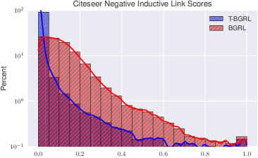
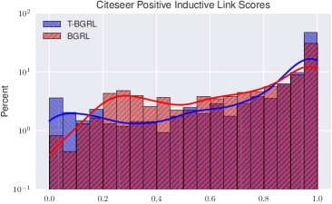
Figure 2: These plots show similarities between node embeddings on Citeseer. Left: distribution of similarity to non-neighbors for T-BGRL and BGRL. Right: distribution of similarity to neighbors for T-BGRL and BGRL. Note that the y-axis is on a logarithmic scale. T-BGRL clearly does a better job of ensuring that negative link representations are pushed far apart from those of positive links.

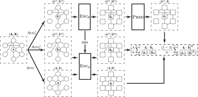
Figure 3: T-BGRL architecture diagram. The loss function is also shown in Equation 5.

In order to reduce this systematic gap in performance between ML-GCN (the best-performing contrastive model) and BGRL (the best-performing non-contrastive model), we observe that we need to push negative and positive node pair representations further apart. This way, pairs between new nodes—introduced at inference time—have a higher chance of being classified correctly. Contrastive methods utilize negative sampling for this purpose, but we wish to avoid negative sampling owing to high computational cost. In lieu of this, we propose a simple, yet powerfully effective idea below.

⬇

# Enc_o: online encoder network

# Enc_t: target encoder network

# Pred: predictor network

# lam: trade-off

# decay: EMA decay parameter

# g: input graph

# feat: node features

g1, feat1 = augment(g, feat) # augmentation #1

g2, feat2 = augment(g, feat) # augmentation #2

c_g, c_feat = corrupt(g, feat) # corruption

h1 = Enc_o(g1, feat1)

h2 = Enc_t(g2, feat2)

c_z = Enc_t(c_g, c_feat)

z1 = Pred(z1)

loss = lam*cosine_similarity(z1, c_z) \

- (1-lam)*cosine_similarity(z1, h2)

loss.backward() # backprop

# Update Enc_t with EMA

Enc_t.params = decay * Enc_t.params \

+ (1-decay) * Enc_o.params

Algorithm 1 PyTorch-style pseudocode for T-BGRL

Model Intuition. To emulate the effect of negative sampling without actually performing it, we propose Triplet-BGRL (T-BGRL). In addition to the two augmentations performed during standard non-contrastive SSL training, we add a corruption to function as a cheap negative sample. For each node, like BGRL, we minimize the distance between its representations across two augmentations. However, taking inspiration from triplet-style losses (Hoffer & Ailon, 2014), we also maximize the distance between the augmentation and corruption representations.

Model Design. Ideally, this model should not only perform better than BGRL in the inductive setting, but should also have the same time complexity as BGRL. In order to meet these expectations, we design efficient, linear-time corruptions (same asymptotic runtime as the augmentations). We also choose to use the online encoder $\textsc{Enc}_{\phi}$ to generate embeddings for the corrupted graph so that T-BGRL does not have any additional parameters. Figure 3 illustrates the overall architecture of the proposed T-BGRL, and Algorithm 1 presents PyTorch-style pseudocode. Our new proposed loss function is as follows:

$${\mathcal{L}}_{{\textsf{T-BGRL}}{}}=\underbrace{\frac{\lambda}{n}\sum^{n-1}_{i=0}\frac{\tilde{{\bm{z}}}_{i}\cdot\check{{\bm{h}}}_{i}}{||\tilde{{\bm{z}}}_{i}||\ ||\check{{\bm{h}}}_{i}||}}_{{\textsf{T-BGRL}}{}\text{ Loss Term}}\underbrace{-\frac{(1-\lambda)}{n}\sum^{n-1}_{i=0}\frac{\tilde{{\bm{z}}}_{i}\cdot{\bm{h}}_{i}^{(2)}}{||\tilde{{\bm{z}}}_{i}||\ ||{\bm{h}}_{i}^{(2)}||}}_{\text{BGRL Loss}}$$ (5)

where $\lambda$ is a hyperparameter controlling the repulsive forces between augmentation and corruption.

Corruption Choice. We experiment with several different corruptions methods, but limit ourselves to linear-time corruptions in order to maintain the efficiency of BGRL. We find that ${\textsc{ShuffleFeatRandomEdge}}({\bm{A}},{\bm{X}})=(\check{{\bm{A}}},\check{{\bm{X}}})$, where $\check{{\bm{A}}}{\sim}\{0,1\}^{n\times n}$ and $\check{{\bm{X}}}=\textsc{ShuffleRows}({\bm{X}})$ works the best. We describe each of the different corruptions we experimented with in Section A.7.

Inductive Results. Table 2 shows that T-BGRL improves inductive performance over BGRL in 5/6 datasets, with very large improvements in the Cora and Citeseer datasets. The only dataset where BGRL outperformed T-BGRL is the Amazon-Photos dataset. However, this gap is much smaller (0.01 difference in Hits@50) than the improvements on the other datasets. We plot the scores output by the decoder for unseen negative pairs compared to those for unseen positive pairs in Figure 2. We can see that T-BGRL pushes apart unseen negative and positive pairs much better than BGRL.

Table 3: Transductive performance of T-BGRL compared to ML-GCN and BGRL (same numbers as Table 1 above; full figure in Table 5).

Dataset	ML-GCN	BGRL	T-BGRL
Cora	0.815	0.792	0.773$\pm$0.020
Citeseer	0.771	0.858	0.868$\pm$0.023
Coauthor-Cs	0.787	0.515	0.555$\pm$0.009
Coauthor-Physics	0.810	0.476	0.471$\pm$0.021
Amazon-Computers	0.320	0.346	0.315$\pm$0.015
Amazon-Photos	0.430	0.562	0.517$\pm$0.016

Transductive Results. We also evaluate the performance of T-BGRL in the transductive setting to ensure that it does not significantly reduce performance when compared to BGRL. See Table 3 on the right for the results.

Difference from Contrastive Methods. While our method shares some similarities with contrastive methods, we believe T-BGRL is strictly non-contrastive because it does not require the $O(n^{2})$ sampling from the complement of the edge index used by contrastive methods. This is clearly shown in Figure 4, where T-BGRL and BGRL have similar runtimes and are much faster than GRACE and ML-GCN. The corruption can be viewed as a “negative” augmentation—with the only difference being that it changes the expected label for each link. In fact, one of the corruptions that we consider, SparsifyFeatSparsifyEdge, is essentially the same as the augmentations using by BGRL (except with much higher drop probability). We discuss other corruptions below in Section A.7.

Scalability. We evaluate the runtime of our model on different datasets. Figure 4 shows the running times to fully train a model for different contrastive and non-contrastive methods over 5 different runs. Note that we use a fixed 10,000 epochs for GRACE, CCA-SSG, GBT, BGRL, and T-BGRL, but use early stopping on the ML-GCN with a maximum of 1,000 epochs. We find that (i) T-BGRL is comparable to BGRL in runtime owing to efficient choices of corruptions, (ii) it is about $4.3\times$ faster than GRACE on Amazon-Computers (the largest dataset which GRACE can run on), and (ii) it is $14\times$ faster than ML-GCN. CCA-SSG is the fastest of all the methods but performs the worst. As mentioned above, we do not compare with SEAL (Zhang & Chen, 2018) or other subgraph-based methods due to how slow they are during inference. SUREL (Yin et al., 2022) is ~250× slower, and SEAL (Zhang & Chen, 2018) is about ~3900× slower according to Yin et al. (2022). In conclusion, we find that T-BGRL is roughly as scalable as other non-contrastive methods, and much more scalable than existing contrastive methods.

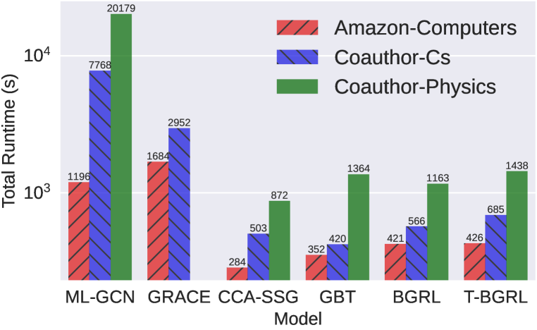
Figure 4: Total runtime comparison of different contrastive and non-contrastive methods. T-BGRL and BGRL have relatively similar runtimes and are significantly faster than the contrastive methods (GRACE and ML-GCN).

5 Other Related Work

Link Prediction. Link prediction is a long-standing graph machine learning task. Some traditional methods include (i) matrix (Menon & Elkan, 2011; Wang et al., 2020) or tensor factorization (Acar et al., 2009; Dunlavy et al., 2011) methods which factor the adjacency and/or feature matrices to derive node representations which can predict links equipped with inner products, and (ii) heuristic methods which score node pairs based on neighborhood and overlap (Yu et al., 2017; Zareie & Sakellariou, 2020; Philip et al., 2010). Several shallow graph embedding methods (Grover & Leskovec, 2016; Perozzi et al., 2014) which train node embeddings by random-walk strategies have also been used for link prediction. In addition to the node-embedding-based GNN methods mentioned in Section 2, several works (Yin et al., 2022; Zhang & Chen, 2018; Hao et al., 2020) propose subgraph-based methods for this task, which aim to classify subgraphs around each candidate link. Few works focus on scalable link prediction with distillation (Guo et al., 2022b), decoder (Wang et al., 2022), and sketching designs (Chamberlain et al., 2022).

Graph SSL Methods. Most graph SSL methods can be put categorized into contrastive and non-contrastive methods. Contrastive learning has been applied to link prediction with margin-loss-based methods such as PinSAGE (Ying et al., 2018a), and GraphSAGE (Hamilton et al., 2017), where negative sample representations are pushed apart from positive sample representations. GRACE (Zhu et al., 2020) uses augmentation (Zhao et al., 2022a) during this negative sampling process to further increase the performance of the model. DGI (Veličković et al., 2018) leverages mutual information maximization between local patch and global graph representations. Some works (Ju et al., 2022; Jin et al., 2021) also explore using multiple contrastive pretext tasks for SSL. Several works (You et al., 2020; Lin et al., 2022) also focus on graph-level contrastive learning, via graph-level augmentations and careful negative selection. Recently, non-contrastive methods have been applied to graph representation learning. Self-GNN (Kefato & Girdzijauskas, 2021) and BGRL (Thakoor et al., 2022) use ideas from BYOL (Grill et al., 2020) and SimSiam (Chen & He, 2021) to propose an graph framework that does not require negative sampling. We describe BGRL in depth in Section 2 above. Graph Barlow Twins (GBT) (Bielak et al., 2022) is adapted from the Barlow Twins model in the image domain (Zbontar et al., 2021), and uses cross-correlation to learn node representations with a shared encoder. CCA-SSG (Zhang et al., 2021) uses ideas from Canonical Correlation Analysis (CCA) (Hotelling, 1992) and Deep CCA (Andrew et al., 2013) for their loss function. These models are somewhat similar in that it has also been shown that Barlow Twins is equivalent to Kernel CCA (Balestriero & LeCun, 2022).

6 Conclusion

To our knowledge, this is the first work to study non-contrastive SSL methods and their performance on link prediction. We first evaluate several contrastive and non-contrastive graph SSL methods on link prediction tasks, and find that surprisingly, one popular non-contrastive method (BGRL) is able to perform well in the transductive setting. We also observe that BGRL struggles in the inductive setting, and identify that it has a tendency to overfit the training graph, indicating it fails to push positive and negative node pair representations far apart from each other. Armed with these insights, we propose T-BGRL, a simple but effective non-contrastive strategy which works by generating extremely cheap “negatives” by corrupting the original inputs. T-BGRL sidesteps the expensive negative sampling step evident in contrastive learning, while enjoying strong performance benefits. T-BGRL improves on BGRL’s inductive performance in 5/6 datasets while achieving similar transductive performance, making it comparable to the best contrastive baselines, but with a 14× speedup over the best contrastive methods.

Reproducibility Statement

To ensure reproducibility, our source code is available online at https://github.com/snap-research/non-contrastive-link-prediction. The hyperparameters and instructions for reproducing all experiments are provided in the README.md file.

Acknowledgments

UCR coauthors were partly supported by the National Science Foundation under CAREER grant no. IIS 2046086 and were also sponsored by the Combat Capabilities Development Command Army Research Laboratory under Cooperative Agreement Number W911NF-13-2-0045 (ARL Cyber Security CRA). Any opinions, findings, and conclusions or recommendations expressed in this material are those of the author(s) and do not necessarily reflect the views of the funding parties.

Appendix A Appendix

A.1 Dataset Statistics

Table 4: Statistics for the datasets used in our work.

Dataset	Nodes	Edges	Features
Cora	2,708	5,278	1,433
Citeseer	3,327	4,552	3,703
Coauthor-Cs	18,333	163,788	6,805
Coauthor-Physics	34,493	495,924	8,415
Amazon-Computers	13,752	491,722	767
Amazon-Photos	7,650	238,162	745

A.2 Machine Details

We run all of our experiments on either NVIDIA P100 or V100 GPUs. We use machines with 12 virtual CPU cores and 24 GB of RAM for the majority of our experiments. We exclusively use V100s for our timing experiments. We ran our experiments on Google Cloud Platform.

A.3 Transductive Setting Details

We use a 85/5/10 split for training/validation/testing data—following Zhang & Chen (2018); Cai et al. (2020).

A.4 Inductive Setting Details

The inductive setting represents a more realistic setting than the transductive setting. For example, consider a social network upon which a model is trained at some time $t_{1}$ but is used for inference (for a GNN, this refers to the message-passing step) at time $t_{2}$, where new users and friendships have been added to the network in the interim. Then, the goal of a model run at time $t_{2}$ would be to predict any new links at new network state $t_{3}$ (although we assume there are no new nodes introduced at that step since we cannot compute the embedding of nodes without performing inference on them first). To simulate this setting, we first perform the following steps:

1. We withhold a portion of the edges (and same number of disconnected node pairs) to use as testing-only edges.

2. We partition the graph into two sets of nodes: “observed” nodes (that we see during training) and “unobserved nodes” (that can only be seen during testing).

3. We mask out some edges to use as testing-only edges.

4. We mask out some edges to use as inference-only edges.

5. We mask out some edges to use as validation-only edges.

6. We mask out some edges to use as training-only edges.

As the test edges are sampled before the node split, there will be three kinds of them after the splitting. Specifically: edges within observed nodes, edges between observed nodes and unobserved nodes, and edges within unobserved nodes. For the ease of data preparation, we use the same percentages for the test edge splitting, unobserved node splitting, and validation edge splitting. Specifically, we mask out 30% of the edges (at each of the above stages) on the small datasets (Cora and Citeseer), and 10% on all the other datasets. We use a 30% split on the small datasets to ensure that we have a sufficient number of edges for testing and validation purposes.

A.5 Experimental Setup

To ensure that we fairly evaluate each model, we run a Bayesian hyperparameter sweep for 25 runs across each model-dataset combination with the target metric being the validation Hits@50. Each run is the result of the mean averaged over 5 runs (retraining both the encoder and decoder). We used the Weights and Biases (Biewald, 2020) Bayesian optimizer for our experiments. We provide a sample configuration file to reproduce our sweeps, as well as the exact parameters used for the top T-BGRL runs shown in our tables.

We used the reference GRACE implementation and BGRL implementation, but modified them for link prediction instead of node classification. We based our E2E-GCN off of the OGB (Hu et al., 2020) implementation. We re-implemented CCA-SSG and GBT. The code for all of our implementations and modifications can be found in the link in our paper above.

A.6 Full Results

Table 5 shows the results of all the methods (including T-BGRL) on transductive setting.

Table 5: Full transductive performance table (combination of Tables 1 and 3).

	End-To-End	Contrastive		Non-Contrastive
Dataset	E2E-GCN	ML-GCN	GRACE	CCA-SSG	GBT	BGRL	T-BGRL
Cora	0.816$\pm$0.013	0.815$\pm$0.002	0.686$\pm$0.056	0.348$\pm$0.091	0.460$\pm$0.149	0.792$\pm$0.015	0.773$\pm$0.020
Citeseer	0.822$\pm$0.017	0.771$\pm$0.020	0.707$\pm$0.068	0.249$\pm$0.168	0.472$\pm$0.196	0.858$\pm$0.020	0.868$\pm$0.023
Amazon-Photos	0.642$\pm$0.029	0.430$\pm$0.032	0.486$\pm$0.025	0.369$\pm$0.013	0.434$\pm$0.038	0.562$\pm$0.013	0.517$\pm$0.016
Amazon-Computers	0.426$\pm$0.036	0.320$\pm$0.060	0.240$\pm$0.027	0.201$\pm$0.032	0.258$\pm$0.008	0.346$\pm$0.018	0.315$\pm$0.015
Coauthor-Cs	0.762$\pm$0.010	0.787$\pm$0.011	0.456$\pm$0.066	0.229$\pm$0.018	0.298$\pm$0.033	0.515$\pm$0.016	0.555$\pm$0.009
Coauthor-Physics	0.798$\pm$0.018	0.810$\pm$0.003	OOM	0.157$\pm$0.009	0.187$\pm$0.011	0.476$\pm$0.015	0.471$\pm$0.021

A.7 Corruptions

In this work, we experiment with the following corruptions:

1. RandomFeatRandomEdge: Randomly generate an adjacency matrix $\tilde{{\bm{A}}}$ and $\tilde{{\bm{X}}}$ with the same sizes as ${\bm{A}}$ and ${\bm{X}}$, respectively. Note that $\tilde{{\bm{A}}}$ and ${\bm{A}}$ also have the same number of non-zero entries, i.e., the same number of edges.

2. ShuffleFeatRandomEdge: Randomly shuffle the rows of ${\bm{X}}$, and generate a random $\tilde{{\bm{A}}}$ with the same size as ${\bm{A}}$. Note that $\tilde{{\bm{A}}}$ and ${\bm{A}}$ also have the same number of non-zero entries, i.e., the same number of edges.

3. SparsifyFeatSparsifyEdge: Mask out a large percentage (we chose 95%) of the entries in ${\bm{X}}$ and ${\bm{A}}$.

Of these corruptions, we find that RandomFeatRandomEdge works the best across our experiments.

A.8 AUC-ROC Results

Here we include the area under the ROC curve for each of the different models under both the inductive and transductive settings. Note that we perform early stopping on the validation Hits@50 when training the link prediction model, not on the validation AUC-ROC.

Table 6: Area under the ROC curve for the methods in the transductive setting.

	End-To-End	Contrastive		Non-Contrastive
Dataset	E2E-GCN	ML-GCN	GRACE	CCA-SSG	GBT	BGRL	T-BGRL
Cora	0.911$\pm$0.004	0.893$\pm$0.007	0.883$\pm$0.020	0.647$\pm$0.076	0.736$\pm$0.109	0.911$\pm$0.008	0.910$\pm$0.005
Citeseer	0.922$\pm$0.006	0.891$\pm$0.006	0.863$\pm$0.042	0.661$\pm$0.050	0.755$\pm$0.120	0.934$\pm$0.009	0.953$\pm$0.003
Coauthor-Cs	0.964$\pm$0.005	0.966$\pm$0.001	0.961$\pm$0.003	0.758$\pm$0.047	0.894$\pm$0.017	0.959$\pm$0.002	0.956$\pm$0.002
Coauthor-Physics	0.978$\pm$0.001	0.986$\pm$0.000	OOM	0.821$\pm$0.051	0.834$\pm$0.084	0.961$\pm$0.002	0.963$\pm$0.001
Amazon-Computers	0.985$\pm$0.001	0.983$\pm$0.001	0.951$\pm$0.011	0.907$\pm$0.025	0.946$\pm$0.007	0.969$\pm$0.002	0.976$\pm$0.001
Amazon-Photos	0.989$\pm$0.000	0.983$\pm$0.002	0.981$\pm$0.001	0.939$\pm$0.008	0.956$\pm$0.015	0.980$\pm$0.000	0.982$\pm$0.000

Table 7: AUC-ROC of various methods in the inductive setting. See Section 3.1.2 for an explanation of our inductive setting.

	End-To-End	Contrastive		Non-Contrastive
Dataset	E2E-GCN	ML-GCN	GRACE	GBT	CCA-SSG	BGRL	T-BGRL
Overall
Cora	0.788$\pm$0.015	0.842$\pm$0.008	0.858$\pm$0.012	0.704$\pm$0.032	0.595$\pm$0.035	0.814$\pm$0.022	0.920$\pm$0.008
Citeseer	0.810$\pm$0.016	0.873$\pm$0.004	0.886$\pm$0.010	0.691$\pm$0.007	0.621$\pm$0.070	0.891$\pm$0.006	0.954$\pm$0.003
Coauthor-Cs	0.881$\pm$0.040	0.956$\pm$0.001	0.944$\pm$0.001	0.875$\pm$0.036	0.831$\pm$0.068	0.968$\pm$0.001	0.958$\pm$0.001
Coauthor-Physics	0.957$\pm$0.004	0.976$\pm$0.001	OOM	0.818$\pm$0.092	0.614$\pm$0.050	0.974$\pm$0.001	0.976$\pm$0.001
Amazon-Computers	0.974$\pm$0.009	0.981$\pm$0.001	0.972$\pm$0.012	0.919$\pm$0.023	0.910$\pm$0.031	0.980$\pm$0.002	0.982$\pm$0.002
Amazon-Photos	0.976$\pm$0.003	0.982$\pm$0.001	0.977$\pm$0.002	0.962$\pm$0.011	0.885$\pm$0.057	0.984$\pm$0.000	0.981$\pm$0.001
Performance on Observed-Observed Node Edges
Cora	0.827$\pm$0.011	0.834$\pm$0.010	0.883$\pm$0.010	0.714$\pm$0.034	0.584$\pm$0.047	0.800$\pm$0.025	0.929$\pm$0.005
Citeseer	0.792$\pm$0.014	0.840$\pm$0.013	0.905$\pm$0.012	0.705$\pm$0.019	0.635$\pm$0.078	0.875$\pm$0.006	0.956$\pm$0.005
Coauthor-Cs	0.886$\pm$0.037	0.951$\pm$0.001	0.947$\pm$0.002	0.874$\pm$0.037	0.828$\pm$0.070	0.967$\pm$0.001	0.955$\pm$0.002
Coauthor-Physics	0.959$\pm$0.004	0.976$\pm$0.001	OOM	0.819$\pm$0.091	0.615$\pm$0.049	0.974$\pm$0.001	0.975$\pm$0.001
Amazon-Computers	0.974$\pm$0.010	0.981$\pm$0.001	0.971$\pm$0.012	0.918$\pm$0.024	0.910$\pm$0.030	0.979$\pm$0.002	0.981$\pm$0.002
Amazon-Photos	0.976$\pm$0.003	0.981$\pm$0.001	0.977$\pm$0.002	0.962$\pm$0.011	0.885$\pm$0.055	0.983$\pm$0.000	0.981$\pm$0.001
Performance on Observed-Unobserved Node Edges
Cora	0.741$\pm$0.022	0.844$\pm$0.010	0.840$\pm$0.017	0.696$\pm$0.030	0.602$\pm$0.024	0.818$\pm$0.023	0.912$\pm$0.010
Citeseer	0.841$\pm$0.019	0.901$\pm$0.005	0.877$\pm$0.012	0.687$\pm$0.016	0.610$\pm$0.069	0.904$\pm$0.006	0.955$\pm$0.004
Coauthor-Cs	0.877$\pm$0.045	0.964$\pm$0.001	0.940$\pm$0.001	0.876$\pm$0.036	0.836$\pm$0.067	0.969$\pm$0.001	0.964$\pm$0.001
Coauthor-Physics	0.953$\pm$0.004	0.975$\pm$0.001	OOM	0.817$\pm$0.093	0.612$\pm$0.052	0.975$\pm$0.001	0.976$\pm$0.000
Amazon-Computers	0.974$\pm$0.009	0.981$\pm$0.001	0.973$\pm$0.011	0.921$\pm$0.022	0.909$\pm$0.032	0.980$\pm$0.002	0.982$\pm$0.002
Amazon-Photos	0.977$\pm$0.003	0.983$\pm$0.001	0.977$\pm$0.002	0.963$\pm$0.012	0.884$\pm$0.059	0.986$\pm$0.000	0.981$\pm$0.002
Performance on Unobserved-Unobserved Node Edges
Cora	0.571$\pm$0.043	0.879$\pm$0.016	0.810$\pm$0.019	0.693$\pm$0.039	0.626$\pm$0.040	0.866$\pm$0.024	0.911$\pm$0.011
Citeseer	0.852$\pm$0.047	0.917$\pm$0.021	0.827$\pm$0.029	0.637$\pm$0.052	0.599$\pm$0.062	0.916$\pm$0.012	0.941$\pm$0.011
Coauthor-Cs	0.850$\pm$0.059	0.964$\pm$0.001	0.928$\pm$0.004	0.877$\pm$0.034	0.839$\pm$0.061	0.967$\pm$0.002	0.966$\pm$0.001
Coauthor-Physics	0.949$\pm$0.006	0.978$\pm$0.001	OOM	0.818$\pm$0.091	0.613$\pm$0.056	0.978$\pm$0.001	0.981$\pm$0.001
Amazon-Computers	0.970$\pm$0.010	0.979$\pm$0.001	0.969$\pm$0.011	0.914$\pm$0.022	0.899$\pm$0.035	0.977$\pm$0.002	0.979$\pm$0.003
Amazon-Photos	0.978$\pm$0.004	0.982$\pm$0.002	0.977$\pm$0.002	0.965$\pm$0.011	0.886$\pm$0.063	0.986$\pm$0.001	0.982$\pm$0.003

A.9 Why Does BGRL Not Collapse?

The loss function for BGRL (see Equation 2) is 0 when $h_{i}^{(2)}$ = 0 or $\tilde{{\bm{z}}}_{i}$ = 0. While theoretically possible, this is clearly undesirable behavior since this does not result in useful embeddings. We refer to this case as the model collapsing. It is not fully understood why non-contrastive models do not collapse, but there have been several reasons proposed in the image domain with both theoretical and empirical grounding. Chen & He (2021) showed that the SimSiam architecture requires both the predictor and the stop gradient. This has also been shown to be true for BGRL. Tian et al. (2021) claim that the eigenspace of predictor weights will align with the correlation matrix of the online network under the assumption of a one-layer linear encoder and a one-layer linear predictor. Wen & Li (2022) looked at the case of a two-layer non-linear encoder with output normalization and found that the predictor is often only useful during the learning process, and often converges to the identity function. We did not observe this behavior on BGRL—the predictor is usually significantly different from that of the identity function.

A.10 How Does BGRL Pull Representations Closer Together?

Here we clarify the intuition behind BGRL pulling similar points together. To simplify this analysis, we assume that the predictor is the identity function, which Wen & Li (2022) found is true in the image representation learning setting. Although we have not observed this in the graph setting, this assumption greatly simplifies our analysis and we argue it is sufficient for understanding why BGRL works.

Suppose we have three nodes: an anchor node $u$, a neighbor $v$, and a non-neighbor $w$. That is, we have $(u,v)\in{\mathcal{E}}$, $(u,w)\not\in{\mathcal{E}}$, and $(v,w)\not\in{\mathcal{E}}$. Let ${\bm{u}},{\bm{v}},{\bm{w}}$ be the embeddings for $u,v,w$, respectively (e.g. ${\bm{u}}=\textsc{Enc}(u)$).

Assuming homophily between the nodes, we have ${\bm{u}}\cdot{\bm{v}}<{\bm{u}}\cdot{\bm{w}}$. For ease of visualization, let us project the points in a 2D space. Then, we have the following:

We then apply the two augmentations on $u$, producing $\tilde{u}_{1}=\textsc{Aug}_{1}(u)$ and $\tilde{u}_{2}=\textsc{Aug}_{2}(u)$. For the sake of simplicity, let us assume that we perform edge dropping and feature dropping with the same probability $p$ (in practice, they may be different from each other). We represent the space of possible values for $\tilde{u}_{1}$ and $\tilde{u}_{2}$ as a circle with radius $r$ centered at $u$, where $r$ is controlled by $p$.

The BGRL loss is stated in Equation 2 above, but we rewrite it relative to our anchor $u$ and with our assumption about the predictor:

$${\mathcal{L}}_{u}=-\frac{\tilde{{\bm{u}}}_{1}\cdot\tilde{{\bm{u}}}_{2}}{||\tilde{{\bm{u}}}_{1}||\ ||\tilde{{\bm{u}}}_{2}||}$$ (6)

Minimizing this loss pushes $\tilde{{\bm{u}}}_{1}$ and $\tilde{{\bm{u}}}_{2}$ closer. Let us denote the encoder after one round of optimization as $\textsc{Enc}^{\prime}$. Then:

$$\mathbb{E}\left[||\textsc{Enc}^{\prime}(\textsc{Aug}(u))-\textsc{Enc}^{\prime}(\textsc{Aug}(u))||\right]<\mathbb{E}\left[||\textsc{Enc}(\textsc{Aug}(u))-\textsc{Enc}(\textsc{Aug}(u))||\right]$$ (7)

Note that ${\bm{v}}$ in this example lies within the space of possible augmentations - that is, $v\in{\mathcal{A}}$, where ${\mathcal{A}}$ is the set of all possible values of $\textsc{Aug}(u)$. This means, as we repeat this process, we implicitly push ${\bm{u}}$ and ${\bm{v}}$ closer together - leading to distributions like those shown in Figure 1.

A.11 Additional Plots

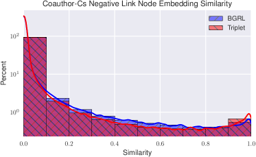
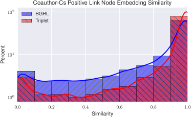
Figure 5: These plots show similarities between node embeddings on Coauthor-Cs. Left: distribution of similarity to non-neighbors for T-BGRL and BGRL (closer to 0 is better). Right: distribution of similarity to neighbors for T-BGRL and BGRL (closer to 1 is better). Note that the y-axis is on a logarithmic scale. T-BGRL clearly does a better job of ensuring that negative link representations are pushed far apart from those of positive links.

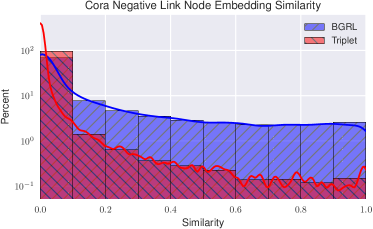
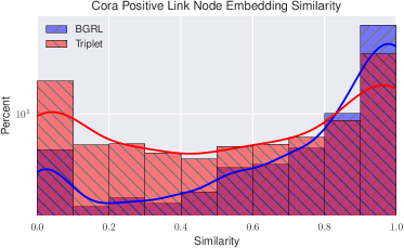
Figure 6: These plots show similarities between node embeddings on Cora. Left: distribution of similarity to non-neighbors for T-BGRL and BGRL (closer to 0 is better). Right: distribution of similarity to neighbors for T-BGRL and BGRL (closer to 1 is better). Note that the y-axis is on a logarithmic scale. T-BGRL clearly does a better job of ensuring that negative link representations are pushed far apart from those of positive links, but does not do as well at differentiating between positive links.

References

- Acar et al. (2009) Evrim Acar, Daniel M. Dunlavy, and Tamara G. Kolda. Link prediction on evolving data using matrix and tensor factorizations. In 2009 IEEE International Conference on Data Mining Workshops, pp. 262–269, 2009. doi: 10.1109/ICDMW.2009.54.
- Andrew et al. (2013) Galen Andrew, Raman Arora, Jeff Bilmes, and Karen Livescu. Deep canonical correlation analysis. In International conference on machine learning, pp. 1247–1255. PMLR, 2013.
- Balestriero & LeCun (2022) Randall Balestriero and Yann LeCun. Contrastive and non-contrastive self-supervised learning recover global and local spectral embedding methods. arXiv preprint arXiv:2205.11508, 2022.
- Berg et al. (2017) Rianne van den Berg, Thomas N Kipf, and Max Welling. Graph convolutional matrix completion. arXiv preprint arXiv:1706.02263, 2017.
- Bielak et al. (2022) Piotr Bielak, Tomasz Kajdanowicz, and Nitesh V. Chawla. Graph barlow twins: A self-supervised representation learning framework for graphs. Knowledge-Based Systems, pp. 109631, 2022. ISSN 0950-7051. doi: https://doi.org/10.1016/j.knosys.2022.109631. URL https://www.sciencedirect.com/science/article/pii/S095070512200822X.
- Biewald (2020) Lukas Biewald. Experiment tracking with weights and biases, 2020. URL https://www.wandb.com/. Software available from wandb.com.
- Cai et al. (2020) Lei Cai, Jundong Li, Jie Wang, and Shuiwang Ji. Line graph neural networks for link prediction, 2020. URL https://arxiv.org/abs/2010.10046.
- Chamberlain et al. (2022) Benjamin Paul Chamberlain, Sergey Shirobokov, Emanuele Rossi, Fabrizio Frasca, Thomas Markovich, Nils Hammerla, Michael M Bronstein, and Max Hansmire. Graph neural networks for link prediction with subgraph sketching. arXiv preprint arXiv:2209.15486, 2022.
- Chen et al. (2019) Chi Chen, Weike Ye, Yunxing Zuo, Chen Zheng, and Shyue Ping Ong. Graph networks as a universal machine learning framework for molecules and crystals. Chemistry of Materials, 31(9):3564–3572, 2019.
- Chen et al. (2018) Hongxu Chen, Hongzhi Yin, Weiqing Wang, Hao Wang, Quoc Viet Hung Nguyen, and Xue Li. Pme: Projected metric embedding on heterogeneous networks for link prediction. In Proceedings of the 24th ACM SIGKDD International Conference on Knowledge Discovery & Data Mining, KDD ’18, pp. 1177–1186, New York, NY, USA, 2018. Association for Computing Machinery. ISBN 9781450355520. doi: 10.1145/3219819.3219986. URL https://doi.org/10.1145/3219819.3219986.
- Chen et al. (2020) Ting Chen, Simon Kornblith, Mohammad Norouzi, and Geoffrey E. Hinton. A simple framework for contrastive learning of visual representations. In ICML, Proceedings of Machine Learning Research, pp. 1597–1607, 2020.
- Chen & He (2021) Xinlei Chen and Kaiming He. Exploring simple siamese representation learning. In Proceedings of the IEEE/CVF Conference on Computer Vision and Pattern Recognition, pp. 15750–15758, 2021.
- Cremonesi et al. (2010) Paolo Cremonesi, Yehuda Koren, and Roberto Turrin. Performance of recommender algorithms on top-n recommendation tasks. In Proceedings of the Fourth ACM Conference on Recommender Systems, RecSys ’10, pp. 39–46, New York, NY, USA, 2010. Association for Computing Machinery. ISBN 9781605589060. doi: 10.1145/1864708.1864721. URL https://doi.org/10.1145/1864708.1864721.
- Derrow-Pinion et al. (2021) Austin Derrow-Pinion, Jennifer She, David Wong, Oliver Lange, Todd Hester, Luis Perez, Marc Nunkesser, Seongjae Lee, Xueying Guo, Brett Wiltshire, et al. Eta prediction with graph neural networks in google maps. In Proceedings of the 30th ACM International Conference on Information & Knowledge Management, pp. 3767–3776, 2021.
- Dunlavy et al. (2011) Daniel M Dunlavy, Tamara G Kolda, and Evrim Acar. Temporal link prediction using matrix and tensor factorizations. ACM Transactions on Knowledge Discovery from Data (TKDD), 5(2):1–27, 2011.
- Fan & Huang (2019) Shuangfei Fan and Bert Huang. Labeled graph generative adversarial networks. arXiv preprint arXiv:1906.03220, 2019.
- Fan et al. (2022) Wenqi Fan, Xiaorui Liu, Wei Jin, Xiangyu Zhao, Jiliang Tang, and Qing Li. Graph trend filtering networks for recommendation. In Proceedings of the 45th International ACM SIGIR Conference on Research and Development in Information Retrieval, pp. 112–121, 2022.
- Grill et al. (2020) Jean-Bastien Grill, Florian Strub, Florent Altché, Corentin Tallec, Pierre Richemond, Elena Buchatskaya, Carl Doersch, Bernardo Avila Pires, Zhaohan Guo, Mohammad Gheshlaghi Azar, et al. Bootstrap your own latent-a new approach to self-supervised learning. Advances in neural information processing systems, 33:21271–21284, 2020.
- Grover & Leskovec (2016) Aditya Grover and Jure Leskovec. node2vec: Scalable feature learning for networks. In KDD, pp. 855–864. ACM, 2016.
- Guo et al. (2021) Zhichun Guo, Chuxu Zhang, Wenhao Yu, John Herr, Olaf Wiest, Meng Jiang, and Nitesh V Chawla. Few-shot graph learning for molecular property prediction. In Proceedings of the Web Conference 2021, pp. 2559–2567, 2021.
- Guo et al. (2022a) Zhichun Guo, Bozhao Nan, Yijun Tian, Olaf Wiest, Chuxu Zhang, and Nitesh V Chawla. Graph-based molecular representation learning. arXiv preprint arXiv:2207.04869, 2022a.
- Guo et al. (2022b) Zhichun Guo, William Shiao, Shichang Zhang, Yozen Liu, Nitesh Chawla, Neil Shah, and Tong Zhao. Linkless link prediction via relational distillation. arXiv preprint arXiv:2210.05801, 2022b.
- Hamilton et al. (2017) William L. Hamilton, Zhitao Ying, and Jure Leskovec. Inductive representation learning on large graphs. In NIPS, pp. 1024–1034, 2017.
- Hao et al. (2020) Yu Hao, Xin Cao, Yixiang Fang, Xike Xie, and Sibo Wang. Inductive link prediction for nodes having only attribute information. In Proceedings of the Twenty-Ninth International Joint Conference on Artificial Intelligence. International Joint Conferences on Artificial Intelligence Organization, jul 2020. doi: 10.24963/ijcai.2020/168. URL https://doi.org/10.24963%2Fijcai.2020%2F168.
- Hassani & Ahmadi (2020) Kaveh Hassani and Amir Hosein Khas Ahmadi. Contrastive multi-view representation learning on graphs. In ICML, volume 119 of Proceedings of Machine Learning Research, pp. 4116–4126. PMLR, 2020.
- He et al. (2020) Xiangnan He, Kuan Deng, Xiang Wang, Yan Li, Yongdong Zhang, and Meng Wang. Lightgcn: Simplifying and powering graph convolution network for recommendation. In Proceedings of the 43rd International ACM SIGIR conference on research and development in Information Retrieval, pp. 639–648, 2020.
- Hoffer & Ailon (2014) Elad Hoffer and Nir Ailon. Deep metric learning using triplet network, 2014. URL https://arxiv.org/abs/1412.6622.
- Hotelling (1992) Harold Hotelling. Relations between two sets of variates. In Breakthroughs in statistics, pp. 162–190. Springer, 1992.
- Hu et al. (2020) Weihua Hu, Matthias Fey, Marinka Zitnik, Yuxiao Dong, Hongyu Ren, Bowen Liu, Michele Catasta, and Jure Leskovec. Open graph benchmark: Datasets for machine learning on graphs. arXiv preprint arXiv:2005.00687, 2020.
- Hubert et al. (2022) Nicolas Hubert, Pierre Monnin, Armelle Brun, and Davy Monticolo. New Strategies for Learning Knowledge Graph Embeddings: the Recommendation Case. In EKAW 2022 - 23rd International Conference on Knowledge Engineering and Knowledge Management, Bolzano, Italy, September 2022. URL https://hal.inria.fr/hal-03722881.
- Jin et al. (2020) Wei Jin, Tyler Derr, Haochen Liu, Yiqi Wang, Suhang Wang, Zitao Liu, and Jiliang Tang. Self-supervised learning on graphs: Deep insights and new direction. arXiv preprint arXiv:2006.10141, 2020.
- Jin et al. (2021) Wei Jin, Xiaorui Liu, Xiangyu Zhao, Yao Ma, Neil Shah, and Jiliang Tang. Automated self-supervised learning for graphs. arXiv preprint arXiv:2106.05470, 2021.
- Ju et al. (2022) Mingxuan Ju, Tong Zhao, Qianlong Wen, Wenhao Yu, Neil Shah, Yanfang Ye, and Chuxu Zhang. Multi-task self-supervised graph neural networks enable stronger task generalization. arXiv preprint arXiv:2210.02016, 2022.
- Kefato & Girdzijauskas (2021) Zekarias T. Kefato and Sarunas Girdzijauskas. Self-supervised graph neural networks without explicit negative sampling. CoRR, abs/2103.14958, 2021. URL https://arxiv.org/abs/2103.14958.
- Kipf & Welling (2017) Thomas N. Kipf and Max Welling. Semi-supervised classification with graph convolutional networks. In ICLR, 2017.
- Lin et al. (2022) Shuai Lin, Chen Liu, Pan Zhou, Zi-Yuan Hu, Shuojia Wang, Ruihui Zhao, Yefeng Zheng, Liang Lin, Eric Xing, and Xiaodan Liang. Prototypical graph contrastive learning. IEEE Transactions on Neural Networks and Learning Systems, 2022.
- Lin et al. (2015) Yankai Lin, Zhiyuan Liu, Maosong Sun, Yang Liu, and Xuan Zhu. Learning entity and relation embeddings for knowledge graph completion. In Proceedings of the Twenty-Ninth AAAI Conference on Artificial Intelligence, AAAI’15, pp. 2181–2187. AAAI Press, 2015. ISBN 0262511290.
- Liu et al. (2022) Gang Liu, Tong Zhao, Jiaxin Xu, Tengfei Luo, and Meng Jiang. Graph rationalization with environment-based augmentations. In Proceedings of the 28th ACM SIGKDD Conference on Knowledge Discovery and Data Mining, pp. 1069–1078, 2022.
- Menon & Elkan (2011) Aditya Krishna Menon and Charles Elkan. Link prediction via matrix factorization. In Joint european conference on machine learning and knowledge discovery in databases, pp. 437–452. Springer, 2011.
- Oord et al. (2018) Aaron van den Oord, Yazhe Li, and Oriol Vinyals. Representation learning with contrastive predictive coding. arXiv preprint arXiv:1807.03748, 2018.
- Perozzi et al. (2014) Bryan Perozzi, Rami Al-Rfou, and Steven Skiena. DeepWalk. In Proceedings of the 20th ACM SIGKDD international conference on Knowledge discovery and data mining. ACM, aug 2014. doi: 10.1145/2623330.2623732. URL https://doi.org/10.1145%2F2623330.2623732.
- Philip et al. (2010) S Yu Philip, Jiawei Han, and Christos Faloutsos. Link mining: Models, algorithms, and applications. Springer, 2010.
- Rendle et al. (2020) Steffen Rendle, Walid Krichene, Li Zhang, and John Anderson. Neural collaborative filtering vs. matrix factorization revisited. In Fourteenth ACM conference on recommender systems, pp. 240–248, 2020.
- Sankar et al. (2021) Aravind Sankar, Yozen Liu, Jun Yu, and Neil Shah. Graph neural networks for friend ranking in large-scale social platforms. In Proceedings of the Web Conference 2021, pp. 2535–2546, 2021.
- Sen et al. (2008) Prithviraj Sen, Galileo Namata, Mustafa Bilgic, Lise Getoor, Brian Galligher, and Tina Eliassi-Rad. Collective classification in network data. AI magazine, 2008.
- Shchur et al. (2018) Oleksandr Shchur, Maximilian Mumme, Aleksandar Bojchevski, and Stephan Gunnemann. Pitfalls of graph neural network evaluation. arXiv preprint arXiv:1811.05868, 2018.
- Shiao & Papalexakis (2021) William Shiao and Evangelos E Papalexakis. Adversarially generating rank-constrained graphs. In 2021 IEEE 8th International Conference on Data Science and Advanced Analytics (DSAA), pp. 1–8. IEEE, 2021.
- Tang et al. (2020) Xianfeng Tang, Yozen Liu, Neil Shah, Xiaolin Shi, Prasenjit Mitra, and Suhang Wang. Knowing your fate: Friendship, action and temporal explanations for user engagement prediction on social apps. In Proceedings of the 26th ACM SIGKDD international conference on knowledge discovery & data mining, pp. 2269–2279, 2020.
- Tang et al. (2022) Xianfeng Tang, Yozen Liu, Xinran He, Suhang Wang, and Neil Shah. Friend story ranking with edge-contextual local graph convolutions. In Proceedings of the Fifteenth ACM International Conference on Web Search and Data Mining, pp. 1007–1015, 2022.
- Thakoor et al. (2022) Shantanu Thakoor, Corentin Tallec, Mohammad Gheshlaghi Azar, Mehdi Azabou, Eva L. Dyer, Rémi Munos, Petar Velickovic, and Michal Valko. Large-scale representation learning on graphs via bootstrapping. In The Tenth International Conference on Learning Representations, ICLR 2022, Virtual Event, April 25-29, 2022. OpenReview.net, 2022. URL https://openreview.net/forum?id=0UXT6PpRpW.
- Tian et al. (2021) Yuandong Tian, Xinlei Chen, and Surya Ganguli. Understanding self-supervised learning dynamics without contrastive pairs, 2021. URL https://arxiv.org/abs/2102.06810.
- Veličković et al. (2018) Petar Veličković, William Fedus, William L. Hamilton, Pietro Liò, Yoshua Bengio, and R Devon Hjelm. Deep graph infomax, 2018. URL https://arxiv.org/abs/1809.10341.
- Wang et al. (2020) Shijie Wang, Guiling Sun, and Yangyang Li. Svd++ recommendation algorithm based on backtracking. Information, 11(7):369, 2020.
- Wang et al. (2022) Yiwei Wang, Bryan Hooi, Yozen Liu, Tong Zhao, Zhichun Guo, and Neil Shah. Flashlight: Scalable link prediction with effective decoders. arXiv preprint arXiv:2209.10100, 2022.
- Wang et al. (2021) Zhitao Wang, Yong Zhou, Litao Hong, Yuanhang Zou, and Hanjing Su. Pairwise learning for neural link prediction. arXiv preprint arXiv:2112.02936, 2021.
- Wen & Li (2022) Zixin Wen and Yuanzhi Li. The mechanism of prediction head in non-contrastive self-supervised learning. arXiv preprint arXiv:2205.06226, 2022.
- Yang et al. (2020) Zhen Yang, Ming Ding, Chang Zhou, Hongxia Yang, Jingren Zhou, and Jie Tang. Understanding negative sampling in graph representation learning, 2020. URL https://arxiv.org/abs/2005.09863.
- Yin et al. (2022) Haoteng Yin, Muhan Zhang, Yanbang Wang, Jianguo Wang, and Pan Li. Algorithm and system co-design for efficient subgraph-based graph representation learning. Proceedings of the VLDB Endowment, 15(11):2788–2796, 2022.
- Ying et al. (2018a) Rex Ying, Ruining He, Kaifeng Chen, Pong Eksombatchai, William L. Hamilton, and Jure Leskovec. Graph convolutional neural networks for web-scale recommender systems. In Proceedings of the 24th ACM SIGKDD International Conference on Knowledge Discovery & Data Mining. ACM, jul 2018a. doi: 10.1145/3219819.3219890. URL https://doi.org/10.1145%2F3219819.3219890.
- Ying et al. (2018b) Rex Ying, Ruining He, Kaifeng Chen, Pong Eksombatchai, William L Hamilton, and Jure Leskovec. Graph convolutional neural networks for web-scale recommender systems. In Proceedings of the 24th ACM SIGKDD international conference on knowledge discovery & data mining, pp. 974–983, 2018b.
- You et al. (2018) Jiaxuan You, Rex Ying, Xiang Ren, William Hamilton, and Jure Leskovec. Graphrnn: Generating realistic graphs with deep auto-regressive models. In International conference on machine learning, pp. 5708–5717. PMLR, 2018.
- You et al. (2020) Yuning You, Tianlong Chen, Yongduo Sui, Ting Chen, Zhangyang Wang, and Yang Shen. Graph contrastive learning with augmentations. Advances in Neural Information Processing Systems, 33:5812–5823, 2020.
- Yu et al. (2017) Chuanming Yu, Xiaoli Zhao, Lu An, and Xia Lin. Similarity-based link prediction in social networks: A path and node combined approach. Journal of Information Science, 43(5):683–695, 2017.
- Zareie & Sakellariou (2020) Ahmad Zareie and Rizos Sakellariou. Similarity-based link prediction in social networks using latent relationships between the users. Scientific Reports, 10(1):1–11, 2020.
- Zbontar et al. (2021) Jure Zbontar, Li Jing, Ishan Misra, Yann LeCun, and Stéphane Deny. Barlow twins: Self-supervised learning via redundancy reduction, 2021. URL https://arxiv.org/abs/2103.03230.
- Zhang et al. (2021) Hengrui Zhang, Qitian Wu, Junchi Yan, David Wipf, and Philip S Yu. From canonical correlation analysis to self-supervised graph neural networks. Advances in Neural Information Processing Systems, 34:76–89, 2021.
- Zhang & Chen (2018) Muhan Zhang and Yixin Chen. Link prediction based on graph neural networks. In Advances in Neural Information Processing Systems, pp. 5165–5175, 2018.
- Zhang & Chen (2019) Muhan Zhang and Yixin Chen. Inductive matrix completion based on graph neural networks. arXiv preprint arXiv:1904.12058, 2019.
- Zhang et al. (2020) Ziwei Zhang, Peng Cui, and Wenwu Zhu. Deep learning on graphs: A survey. IEEE Transactions on Knowledge and Data Engineering, 2020.
- Zhao et al. (2022a) Tong Zhao, Wei Jin, Yozen Liu, Yingheng Wang, Gang Liu, Stephan Günneman, Neil Shah, and Meng Jiang. Graph data augmentation for graph machine learning: A survey. arXiv preprint arXiv:2202.08871, 2022a.
- Zhao et al. (2022b) Tong Zhao, Gang Liu, Daheng Wang, Wenhao Yu, and Meng Jiang. Learning from counterfactual links for link prediction. In International Conference on Machine Learning, pp. 26911–26926. PMLR, 2022b.
- Zhu et al. (2020) Yanqiao Zhu, Yichen Xu, Feng Yu, Qiang Liu, Shu Wu, and Liang Wang. Deep graph contrastive representation learning. arXiv preprint arXiv:2006.04131, 2020.