Semi-empirical quantum chemical approaches are known to compromise accuracy for feasibility of calculations on huge molecules. However, the need for ultrafast calculations in interactive quantum mechanical studies, high-throughput virtual screening, and for data-driven machine learning has shifted the emphasis towards calculation runtimes recently. This comes with new constraints for the software implementation as many fast calculations would suffer from a large overhead of manual setup and other procedures that are comparatively fast when studying a single molecular structure, but which become prohibitively slow for high-throughput demands. In this work, we discuss the effect of various well-established semi-empirical approximations on calculation speed and relate this to data transfer rates from the raw-data source computer to the results visualization front end. For the former, we consider desktop computers, local high performance computing, as well as remote cloud services in order to elucidate the effect on interactive calculations, for web and cloud interfaces in local applications, and in world-wide interactive virtual sessions. The models discussed in this work have been implemented into our open-source software SCINE Sparrow.

1 Introduction

Semi-empirical methods have originated as feasible quantum chemical approaches at times when computer hardware was struggling with advanced ab initio methods (and even with Hartree–Fock calculations). The advancement of modern computer hardware in the past three decades has not rendered semi-empirical approaches superfluous, but instead pushed the limits of molecular size that can be considered in a single electronic structure calculation (not requiring any embedding techniques, which would introduce further approximations of different flavor into the first-principles calculations). In recent years, several research groups have successfully carried out semi-empirical calculations for systems exceeding thousands of atoms. For example, Hennemann and Clark reported a calculation on no fewer than 100’000 atoms with their EMPIRE code¹. Dral presented results for carbon nanotubes and carbon peapods with about 1000 atoms². Thiel and coworkers developed a computer program accelerated by graphical processing units (GPUs), able to carry out calculations on systems with more than 1000 heavy atoms (e.g., a water cluster consisting of 1800 H₂O molecules)³. A similar approach was taken by Maia et al., who extended the MOPAC program to take advantage of GPUs. With the resulting software, these authors could also successfully carry out calculations for systems with more than 1000 atoms⁴. Recently, Tretiak and coworkers described PYSEQM, a computer program for Born–Oppenheimer molecular dynamics based on semi-empirical methods; they presented results for a phenylene–ethynylene dendrimer consisting of 884 atoms⁵. Stewart demonstrated a calculation on a protein with 14’566 atoms⁶. Also the DFTB+ software package, implementing density functional tight binding methods, can be applied to systems with 1000 atoms and more⁷.

Due to their short runtimes, semi-empirical methods allow one to conduct high-throughput virtual screening campaigns^{8, 9} on very large molecule sets in comparatively little time. For example, Halls and Tasaki screened more than 7000 compounds for the suitability as lithium ion battery additives with the PM3 model¹⁰. Jensen and coworkers presented a workflow based on the PM6 model to predict pK_a values which is fast enough to be used in screening studies with as few as one hundred processors¹¹. Zwijnenburg and coworkers proposed a high-throughput screening approach to assess optoelectronic properties of conjugated polymers which is based on the xTB model^{12, 13}. Wen et al. assessed the detonation velocity of about 100’000 high-energy materials with the PM7 model¹⁴.

In many cases, semi-empirical methods are employed in high-throughput screening studies as part of more complex workflows. For example, structures can be preoptimized with a fast semi-empirical calculation and then subsequently refined with a more accurate albeit computationally more costly method, or compound structures can be entirely determined with semi-empirical methods while some desired property is evaluated with a more accurate electronic structure model (see, e.g., Refs. 15, 16, 17, 18, 19, 20, 21, 22, 23).

The rise of data-driven machine learning approaches in computational chemistry also gives a substantial impetus for the application of semi-empirical methods, both for data generation and for developing new hybrid machine learning/semi-empirical methods. Data-driven approaches are hungry for data and fast semi-empirical methods allow for generating vast amounts of data within a reasonable amount of time (e.g., PM6 was used to calculate optimized molecular geometries and electronic properties of 221 million molecules²⁴ and, earlier, PM7 was used to preoptimize structures of 134 thousand molecules in the QM9 dataset²³). Pure machine learning models are faster than semi-empirical methods but suffer from poorer transferability. The combination of machine learning with physics-based semi-empirical methods creates more transferable hybrid methods that can target higher accuracy approaches (mostly, density functional theory^{25, 26, 27, 28, 29, 30, 31}, but also a few methods^{32, 33} such as AIQM1³³ targeting coupled cluster or G4MP2 accuracy; see the recent overview in Ref. 34). For instance, AIQM1 turned out to be computationally faster and at the same time more accurate than many standard density functional theory methods for various applications and even helped to revise experimental data^{33, 35}.

An important area of application for ultrafast semi-empirical methods is interactive quantum mechanics^{36, 37, 38, 39}. Behind this approach is haptic quantum chemistry⁴⁰ which exploits the tactile human sense so that a person can manipulate a molecule of interest in real time (e.g., try to abstract a proton) while the structure is continuously relaxed. For a realistic experience, it is important that this relaxation is carried out in a physically meaningful way, i.e., according to the laws of quantum mechanics. Furthermore, it needs to be fast enough so as not to break the interactivity. For a fluent visual feedback, about 30 – 60 calculations need to finish sequentially per second, while direct haptic (i.e., tactile) feedback requires, in principle, up to 1000 single-point calculations per second, which can, however, be reduced to a smaller number through activation of a mediator potential⁴¹. Semi-empirical methods are generally fast compared to full-fledge electronic structure models, which makes them therefore ideally suited for interactive applications.

Last but not least, we note that very fast quantum chemical calculations are also a key ingredient to ab initio molecular dynamics⁴², where long trajectories with femtosecond timestep resolution demand fast electronic structure programs to make thousands of single-point calculations viable.

Approaches to reduce the computational complexity of a given quantum chemical method, in particular linear-scaling approaches, obviously play an important role in the acceleration of quantum chemical calculations^{43, 44, 45, 46}. However, it is important to realize that such approaches are primarily targeting atomistic systems of increasing size. For small and medium-sized molecules, the overall calculation time might not be significantly reduced with respect to a canonical approach. This is an important observation, because especially for interactive applications the absolute calculation time is decisive rather than the relative scaling of a method. It is for this reason that our focus here will be on the actual, overall computation time of the methods discussed.

In this work, we report the implementation of a particular class of semi-empirical methods, the so-called orthogonalization-corrected methods (OMx)^{47, 48, 49, 50, 51, 52, 53}, as well as AIQM1, an artificial intelligence-enhanced method based on OMx, into our software package SCINE Sparrow^{54, 55}. In addition, we investigate runtimes of various semi-empirical methods implemented in Sparrow and relate them to transmission times of various computer networks. In particular for interactive applications, these transmission times are an important factor to consider. This allows us to investigate the suitability of different combinations of semi-empirical methods and computing environments for high-throughput screening as well as interactive settings for various molecule sizes.

This work is organized as follows: In section 2, we review the central approximations for the various classes of semi-empirical methods available in Sparrow. Particular emphasis is placed on the OMx methods. Then, we detail the computational methodology adopted in this work and present and analyze runtimes measured and relate them to the constraints set by interactive quantum mechanics and by high-throughput computational campaigns in section 3. Finally, we draw conclusions in section 4.

2 Theory

In this section, we give a brief overview of the various semi-empirical methods implemented in Sparrow which are summarized in Table 1. For a more general introduction on semi-empirical methods we refer the reader to the recent review in Ref. 56.

Table 1: Overview of the methods implemented in Sparrow.

Method	Parametrized elements	Analytical gradients	Reference
Density functional tight binding
DFTB0	H, B – F, Si – Cl, Br, I,	yes	57, 58
	Na, Mg, K – Ti, Fe – Ni, Zna
DFTB2	H, B – F, Si – Cl, Br, I,	yes	59
	Na, Mg, K – Ti, Fe – Ni, Zna
DFTB3	H, B – F, Si – Cl, Br, I,	yes	60
	Na, Mg, K – Ti, Fe – Ni, Zna
Neglect of Diatomic Differential Overlap (MNDO-type)
MNDO(/d)	H-Ca, Zn-Sr, In-Ba, Hg-Bi	yes	61, 62
AM1	H-Be, C-Ca	yes	63
RM1	H, C-F, P-Cl, Br, I	yes	64
PM3	H-Ca, Zn-Sr, Cd-Ba, Hg-Bi	yes	65, 66
PM6	H-Bi except Ce-Lub	yes	67
Neglect of Diatomic Differential Overlap
(orthogonalization-corrected and machine learning-enhanced)
OM2	H, C, N, O, F	no	49, 50, 52
OM3	H, C, N, O, F	no	51, 52
AIQM1	H, C, N, O	no	33
a Depending on the actual parameter set employed, parameters for some elements
will usually not be available in a given calculation (see Section 2.1.2).
b For some pairs of elements some parameters are not available.

2.1 Semi-Empirical Models and their Intricate Parameter Dependence

2.1.1 Neglect of Diatomic Differential Overlap

The basic Hartree–Fock approach toward the solution of the nonrelativistic Schrödinger equation formally scales with the fourth power of the number of single-particle basis functions. This scaling was a severe bottleneck for the limited computational resources available in the 1960s and 1970s, which is why semi-empirical methods were developed by introducing rather drastic approximations.

An important class of semi-empirical models is based on the neglect of diatomic differential overlap (NDDO) that makes three key approximations. First, the number of explicitly considered electrons is reduced to a minimum. For example, for carbon, only four electrons are considered explicitly; the two $1s$-type core electrons are treated implicitly. In fact, the number of valence electrons considered explicitly is never larger than 12, for any element.

Second, the number of basis functions is reduced to the absolute minimum by relying on minimal basis sets. For example, for carbon, only an $s$-type and three $p$-type functions are used.

Third, the NDDO approximation itself is adopted to approximate the electron-repulsion integrals (ERIs),

$$\langle\phi_{\mu}\phi_{\nu}|\phi_{\lambda}\phi_{\sigma}\rangle\approx\delta_{\rm IJ}\delta_{\rm KL}\langle\chi_{\mu}^{\rm I}\chi_{\nu}^{\rm J}|\chi_{\lambda}^{\rm K}\chi_{\sigma}^{\rm L}\rangle.$$ (1)

Here, $\phi_{\mu}$ is the $\mu$th orthogonalized basis function and $\chi_{\mu}^{I}$ is the $\mu$th atomic basis function centered on atom I. Any ERI for which basis functions $\mu$ and $\nu$ as well as $\lambda$ and $\sigma$ are not located on the same atom are neglected, hence lowering the scaling from the fourth to the second power in the number of basis functions.

During the past decades a range of models has been developed based on these three core approximations. Notable examples are MNDO⁶¹, MNDO/d⁶², AM1⁶³, RM1⁶⁴, PM3^{65, 66}, PM6⁶⁷, and PM7⁶⁸ as well as the family of orthogonalization-corrected methods described below. For a more detailed introduction into the NDDO approximation and the multitude of models applying it, we refer the reader to the review in Ref. 55. Sparrow implements MNDO, AM1, RM1, PM3, and PM6⁶⁹. Note that extensions to PM6, such as PM6-DH⁷⁰, PM6-DH2⁷¹, PM6-DH+⁷², and PM6-D3H4⁷³, which aim at improving the description of noncovalent interactions, are currently not available in Sparrow. For MNDO, parameters are supplied for elements H – Ca, Zn – Sr, In – Ba, and Hg – Bi. For AM1, the parameters cover elements H – Be, and C – Ca, while RM1 has parameters for H, C – F, P – Cl, Br, and I. PM3 features parameters for elements H – Ca, Zn – Sr, Cd – Ba, and Hg – Bi. PM6 covers all elements up to Bi except the lanthanides Ce – Lu. Note, however, that not every possible pairwise combination of these elements is parametrized. If parameters are missing for a certain element or element pair, SCINE Sparrow produces an error message, pointing out which parameters are exactly missing. Arbitrary, user-defined parameters can also be supplied.

2.1.2 Density Functional Tight Binding

A different approach is taken by the so-called density functional tight binding (DFTB) family of models⁷⁴. It is based on a Taylor series expansion of the electronic energy around a reference energy based on a superposition of atomic electron densities. With this ansatz, the electronic energy $E^{\rm DFTB}$ is obtained as

$$E^{\rm DFTB}=E_{\rm rep}+\sum_{i}^{\rm occ}\epsilon_{i}+\frac{1}{2}\sum_{\rm A,B}^{N}\Delta q_{\rm A}\Delta q_{\rm B}\gamma_{\rm AB}+\frac{1}{3}\sum_{\rm A,B}^{N}\Delta q_{\rm A}^{2}\Delta q_{\rm B}\Gamma_{\rm AB}+\ldots$$ (2)

Here, $E_{\rm rep}$ models the repulsion energy, whereas the second term represents the binding energy. The latter is based on a linear combination of atomic orbitals and determined from an eigenvalue problem similar to the one appearing in the standard Hartree–Fock model. In its simplest form (sometimes called DFTB0, non-self-consistent DFTB or non-SCC DFTB), only these first two terms are considered^{57, 58}. Both terms are heavily parametrized, and the eigenvalue problem required for the second term does not have to be solved in an iterative fashion (hence the term “non-self-consistent DFTB”).

The third term in Eq. (2) takes into account charge transfer, allowing for a better description of polarized systems. The charge fluctuations on atom A, $\Delta q_{\rm A}$, are determined in a Mulliken population analysis and $\gamma_{\rm AB}$ is a parametrized function of the internuclear distance between atoms A and B. When this third term is also considered, the resulting method is called DFTB2 or self-consistent-charge DFTB (SCC-DFTB)⁵⁹.

Finally, the DFTB3 method⁶⁰ takes into account density fluctuations up to third order by incorporating also the fourth term on the right-hand side of Eq. (2). $\Gamma_{\rm AB}$ is also a parametrized function depending on the internuclear distance. Note that the function $\gamma_{\rm AB}$ is not exactly the same in DFTB3 compared to DFTB2, but contains an additional scaling factor.

Besides these three original DFTB approaches, another class of semi-empirical models based on the tight-binding idea was developed by Grimme and coworkers, namely GFN0-xTB⁷⁵, GFN1-xTB⁷⁶, and GFN2-xTB⁷⁷. These models were developed with a focus on general applicability for almost all elements of the periodic table, which has been a key feature for their fast and widespread acceptance.

Sparrow implements DFTB0, DFTB2, and DFTB3⁶⁹. For these methods, the parameter sets 3ob-1-1 (covering elements C, H, N, and O), 3ob-2-1 (C, H, N, O, P, and S), 3ob-3-1 (covering C, H, N, O, P, S, F, Cl, Br, I, Na, K, Ca, Mg, and Zn), mio-1-1 (C, H, N, O, and S), mio-1-1 (containing C, H, N, O, P, and S), borg-0-1 (H, B), pbc-0-3 (C, H, N, O, Si, F, and Fe), trans3d-0-1 (C, H, N, O, Sc, Ti, Fe, Co, and Ni), and znorg-0-1 (covering C, H, N, O, S, and Zn) are supplied. Other, user-defined parameter sets can also be supplied.

2.1.3 Orthogonalization-Corrected Methods

For the present work, we have implemented in Sparrow orthogonalization-corrected methods (OMx) models: OM2^{50, 49}, OM3⁵¹, ODM2*⁵³, ODM3*⁵³, and AIQM1³³. Other OMx variants not implemented in Sparrow are OM1^{47, 48}, ODM2⁵³, and ODM3⁵³. Different from most traditional NDDO-based semi-empirical molecular orbital methods, such as MNDO⁶¹, AM1⁶³, PM3^{65, 66}, PM6⁶⁷, and PM7⁶⁸, etc., OMx models include orthogonalization corrections, $V^{\text{ORT}}$, in the core Hamiltonian, $H^{\text{core}}$, which is part of the Fock matrix:

$$H_{\mu\nu}^{\text{core\,\,}}=U_{\mu\mu}\delta_{\mu\nu}+\sum_{\text{B}}{\left[V_{\mu\nu,\text{B}}^{\text{s}}+V_{\mu\nu,\text{B}}^{\text{ORT}}+V_{\mu\nu,\text{B}}^{\text{PI}}+V_{\mu\nu,\text{B}}^{\text{ECP}}\right]},$$ (3)

$$H_{\mu\lambda}^{\text{core\,\,}}=\beta_{\mu\lambda}+\sum_{\text{C}}{V_{\mu\lambda,\text{C}}^{\text{ORT}}}.$$ (4)

In addition, the attractive penetration integrals, $V^{\text{PI}}$, and the repulsive effective core potentials, $V^{\text{ECP}}$ are also incorporated into the one-center core Hamiltonian matrix. Here, we follow a common notation to distinguish different centers of basis functions: subscripts $\mu$ and $\upsilon$ denote basis functions centered on the same atom A, while subscript $\lambda$ denotes basis functions at another atom B, which is different from A, and C represents an atom which is neither A, nor B.

The first term $U_{\mu\mu}$ in Eq. (3) is the one-center one-electron energy of atom A and is obtained by parameterization. $V_{\mu\upsilon,B}^{s}$ is the semi-empirical core–electron attraction and calculated as in MNDO-type models:

$$V_{\mu\nu,\text{B}}^{\text{s}}=-Z_{\text{B}}\left(\mu^{\text{A}}\nu^{\text{A}},s^{\text{B}}s^{\text{B}}\right)^{\text{s}},$$ (5)

where $Z_{\text{B}}$ is the core charge of atom B, and the semi-empirical two-center electron ERIs are obtained by multiplying the analytic ERIs $\left(\mu^{\text{A}}\nu^{\text{A}},s^{\text{B}}s^{\text{B}}\right)^{\text{s}}$ with a Klopman–Ohno scaling factor $f_{\text{KO}}$:

$$\left(\mu^{\text{A}}\nu^{\text{A}},\lambda^{\text{B}}\sigma^{\text{B}}\right)^{\text{s}}=f_{\text{KO}}\left(\mu^{\text{A}}\nu^{\text{A}},\lambda^{\text{B}}\sigma^{\text{B}}\right)^{\text{a}}.$$ (6)

The introduction of $f_{\text{KO}}$ ensures that the semi-empirical two-center ERIs smoothly transition to the corresponding values in the one-center limit. It is given by

$$f_{\text{KO}}=\left(s^{\text{A}}s^{\text{A}},s^{\text{B}}s^{\text{B}}\right)^{\text{MNDO}}/\left(s^{\text{A}}s^{\text{A}},s^{\text{B}}s^{\text{B}}\right)^{\text{a}},$$ (7)

where the integrals in the numerator are the MNDO-type ERIs and calculated from semi-empirical multipole-multipole interactions. The core-core repulsion energy is also scaled with the $f_{\text{KO}}$ factor,

$$E_{\text{AB}}^{\text{core\,\,}}=f_{\text{KO}}Z_{\text{A}}Z_{\text{B}}/R_{\text{AB}},$$ (8)

where $R_{\text{AB}}$ is the distance between atoms A and B.

Another key feature of OMx methods is that the minimal valence contracted Gaussian type orbitals (GTOs) instead of Slater type orbitals (STOs) are employed in integral calculations, and a scaling factor $\zeta$ is used to adjust the exponents of the primitive Gaussian functions. That is, an STO-3G contraction is used for hydrogen and ECP-3G for all other elements. Then, the (analytic) ERIs – and also the overlap integrals below – can be evaluated analogously to the full “ab initio” ones with the Libint library⁷⁸ in Sparrow.

In the following, we provide a detailed description of $V^{\text{ORT}}$, $V^{\text{PI}}$, and $V^{\text{ECP}}$ because these three terms are the key ingredients in OMx models (beyond MNDO-type models) and achieve systematic improvements. Moreover, their description is scattered over multiple resources in the original literature, which may hamper the implementation of OMx models.

Orthogonalization corrections $V^{\text{ORT}}$. The inclusion of the orthogonalization correction $V^{\text{ORT}}$ retrieves the effect of a transformation from a nonorthogonal (“atomic-orbital”) basis {$\chi$} to an orthogonal (“molecular-orbital”) basis {$\phi$} by expanding the Löwdin orthogonalization⁷⁹ to second order in terms of overlap integrals:

$${}^{\phi}\boldsymbol{H}=\left({}^{\chi}\boldsymbol{S}\right)^{-\frac{1}{2}}{}^{\chi}\boldsymbol{H}\left({}^{\chi}\boldsymbol{S}\right)^{-\frac{1}{2}}=\left(\mathbf{1}+{}^{\chi}\boldsymbol{S}^{\prime}\right)^{-\frac{1}{2}}{}^{\chi}\boldsymbol{H}\left(\mathbf{1}+{}^{\chi}\boldsymbol{S}^{\prime}\right)^{-\frac{1}{2}},$$ (9)

$${}^{\phi}\boldsymbol{H}\approx {}^{\chi}\boldsymbol{H}-\frac{1}{2}\left({}^{\chi}\boldsymbol{S}^{\prime}{}^{\chi}\boldsymbol{H}+{}^{\chi}\boldsymbol{H}{}^{\chi}\boldsymbol{S}^{\prime}\right)+\frac{3}{8}\left({}^{\chi}\boldsymbol{S}^{\prime 2}{}^{\chi}\boldsymbol{H}+{}^{\chi}\boldsymbol{H}^{\chi}\boldsymbol{S}^{\prime 2}\right)$$ (10)

$$+\frac{1}{4}{}^{\chi}\boldsymbol{S}^{\prime}{}^{\chi}\boldsymbol{H}^{\chi}\boldsymbol{S}^{\prime}+\mathcal{O}\left({}^{\chi}\boldsymbol{S}^{\prime 3}\right),$$

where ${}^{\chi}\boldsymbol{S}^{\prime}={}^{\chi}\boldsymbol{S}-\mathbf{1}$.

Based on Eq. (10), OMx methods adopt different parametric formulae in the the matrix-element calculation of ${}^{\phi}\boldsymbol{H}$. For simplicity, we will neglect the superscripts $\chi$ and $\phi$ in the following.

The very first OMx method OM1 only introduces the one-center orthogonalization corrections $V_{\mu\nu,\mathrm{B}}^{\mathrm{ORT}}$ defined as

$$V_{\mu\nu,\text{B}}^{\text{ORT}}= -\frac{1}{2}F_{1}^{\text{A}}\sum_{\rho\in\text{B}}{\left(S_{\mu\rho}\beta_{\rho\nu}+\beta_{\mu\rho}S_{\rho\nu}\right)}$$ (11)

$$+\frac{1}{8}F_{2}^{\text{A}}\sum_{\rho\in\text{B}}{S_{\mu\rho}}S_{\rho\nu}\left(H_{\mu\mu,\text{B}}+H_{\nu\nu,\text{B}}-2H_{\rho\rho,\text{A}}\right),$$

where $F_{1}$ and $F_{2}$ are element-dependent parameters controlling the magnitudes of the one-center orthogonalization corrections. $S_{\mu\rho}$ and $\beta_{\rho\nu}$ are the overlap and resonance integrals, respectively.

The resonance integrals represent the two-center one-electron integrals $\left\langle\phi_{\mu}^{A}|T+V_{A}+V_{B}|\phi_{\mu}^{B}\right\rangle$ containing kinetic energy and nuclear–electron attraction terms arising from orbitals $\phi_{\mu}^{A}$ and $\phi_{\mu}^{B}$ on atoms A and B. Due to the severe effect of symmetric orthogonalization⁸⁰, they are not evaluated analytically, but by an empirical formula in attempt to recover the orthogonalization effects through parametrization. The empirical formula is different compared to MNDO-based methods and given by^{47, 48}

$$\beta_{\mu\lambda}=\frac{1}{2}\left(\beta_{\mu}^{\text{A}}+\beta_{\lambda}^{\text{B}}\right)\sqrt{R_{\text{AB}}}\exp\left[-\left(\alpha_{\mu}^{\text{A}}+\alpha_{\lambda}^{\text{B}}\right)R_{\text{AB}}^{2}\right],$$ (12)

where $\alpha^{\text{X}}$ and $\beta^{\text{X}}$ are element- and orbital-type-dependent parameters. The resonance integrals are first calculated in a local diatomic coordinate system and then transformed into the global coordinate system.

For $s$, $p_{x}$, $p_{y}$, $p_{z}$ type basis functions, the rotation matrices for this transformation from the local to the global coordinate system have the following form:

$$\boldsymbol{M}^{\text{rot}}=\left[\begin{matrix}1&0&0&0\\ 0&\sin b\cos a&\sin b\sin a&\cos b\\ 0&\cos b\cos a&\cos b\sin a&-\sin b\\ 0&-\sin a&\cos a&0\\ \end{matrix}\right],$$ (13)

where the angle $b$ is defined as the angle between vectors $\boldsymbol{z}$ and $\boldsymbol{z}^{\text{loc}}$, and the angle $a$ is the angle between vector $\boldsymbol{x}$ and the projection of $\boldsymbol{z}^{\text{loc}}$ into the $xy$ plane. The details of the construction of vectors $\boldsymbol{x}^{\text{loc}}$, $\boldsymbol{y}^{\text{loc}}$, $\boldsymbol{z}^{\text{loc}}$ can be found in the Supporting Information of Ref. 55.

Considering the integral elements of matrix $\boldsymbol{I}$ in the local coordinate systems of atoms A and B, their corresponding values in the global coordinate system can be calculated by:

$$\boldsymbol{I}=\begin{cases}\boldsymbol{I}^{\text{loc}},&n_{\text{A}}=n_{\text{B}}=1,\\ \left(\boldsymbol{M}^{\text{rot}}\right)^{T}\boldsymbol{I}^{\text{loc}},&n_{\text{A}}=4,n_{\text{B}}=1,\\ \boldsymbol{I}^{\text{loc}}\boldsymbol{M}^{\text{rot}},&n_{\text{A}}=1,n_{\text{B}}=4,\\ \left(\boldsymbol{M}^{\text{rot}}\right)^{T}\boldsymbol{I}^{\text{loc}}\boldsymbol{M}^{\text{rot}},&n_{\text{A}}=n_{\text{B}}=4,\\ \end{cases}$$ (14)

where $n_{\text{A}}$ and $n_{\text{B}}$ are the number of basis functions on atoms A and B, respectively.

The matrix element $H_{\mu\mu,\mathrm{X}}$ is restricted to an atom pair A–X and is calculated by

$$H_{\mu\mu,\text{X}}=U_{\mu\mu}+V_{\mu\mu,\text{X}}^{\text{s}}.$$ (15)

It should be noted that the second sum in Eq. (11) is implemented by calculating each contribution in a local coordinate system. Hence, a local to global coordinate transformation is required.

In contrast to OM1, OM2 additionally includes two-center orthogonalization corrections $V_{\mu\lambda,\mathrm{C}}^{\mathrm{ORT}}$ in the core Hamiltonian in Eq. (4):

$$V_{\mu\lambda,\text{C}}^{\text{ORT}}= -\frac{1}{2}G_{1}^{\text{AB}}\sum_{\rho\in\text{C}}{\left(S_{\mu\rho}\beta_{\rho\lambda}+\beta_{\mu\rho}S_{\rho\lambda}\right)}$$ (16)

$$+\frac{1}{8}G_{2}^{\text{AB}}\sum_{\rho\in\text{C}}{S_{\mu\rho}}S_{\rho\lambda}\left(H_{\mu\mu,\text{C}}+H_{\lambda\lambda,\text{C}}-H_{\rho\rho,\text{A}}-H_{\rho\rho,\text{B}}\right),$$

where $G_{1}^{\mathrm{AB}}$ and $G_{2}^{\mathrm{AB}}$ are defined as the arithmetic means of element-dependent parameters $G$:

$$G_{1}^{\text{AB}}=\frac{1}{2}\left(G_{1}^{\text{A}}+G_{1}^{\text{B}}\right),$$ (17)

$$G_{2}^{\text{AB}}=\frac{1}{2}\left(G_{2}^{\text{A}}+G_{2}^{\text{B}}\right).$$ (18)

All terms in Equation (16) are directly calculated in the global coordinate system. To ensure rotational invariance, $H_{\mu\mu,\mathrm{X}}$ needs to be averaged when $\mu$ is a $p$-type basis function

$$H_{pp,\text{X}}=\frac{1}{3}\left(H_{xx,\text{X}}+H_{yy,\text{X}}+H_{zz,\text{X}}\right).$$ (19)

Differing from OM2, OM3 neglects the second-order terms in one- and two-center orthogonalization corrections, i.e., both $F_{2}^{\text{X}}$ and $G_{2}^{\text{X}}$ are zeros in OM3.

Penetration integrals $V^{\text{PI}}$. The penetration integrals $V_{\mu\nu,\mathrm{B}}^{\mathrm{PI}}$ are defined as the difference between the actual core–electron attraction integrals, which are obtained from the analytic core–electron attraction integrals $V_{\mu\nu,\mathrm{B}}^{\mathrm{a}}$ scaled by $f_{\mathrm{KO}}$, and their corresponding semi-empirical analogs:

$$V_{\mu\nu,\text{B}}^{\text{PI}}=f_{\text{KO}}V_{\mu\nu,\text{B}}^{\text{a}}-V_{\mu\nu,\text{B}}^{\text{s}}.$$ (20)

In our Sparrow implementation, $V_{\mu\nu,\mathrm{B}}^{\mathrm{a}}$ are evaluated by the integral engine of Libint. Note that there is a slight mistake in the description of the OMx methods in Ref. 55: For the OMx methods, the first two terms of the second sum of Eq. (77) of Ref. 55 always cancel each other. Accordingly, Eq. (80) of Ref. 55 is always fulfilled, not only for s-type orbitals.

Effective core potentials $V^{\text{PI}}$. To account for core–valence interactions, ECP contributions are incorporated into OMx methods. In OM2 and OM3, the following empirical expression is used to calculate $V_{\mu\nu,\mathrm{B}}^{\mathrm{ECP}}$:

$$V_{\mu\nu,\text{B}}^{\text{ECP}}=-\sum_{\alpha\in\text{B}}{\left(S_{\mu\alpha}G_{\alpha\nu}+G_{\mu\alpha}S_{\alpha\nu}+S_{\mu\alpha}S_{\alpha\nu}F_{\alpha\alpha}\right)},$$ (21)

where $F_{\alpha\alpha}$ is treated as an atomic parameter and $G_{\mu\alpha}$ is represented by an expression analogous to the resonance integrals:

$$G_{\mu\alpha}=\frac{1}{2}\left(\beta_{\mu}^{\text{A}}+\beta_{\alpha}^{\text{B}}\right)\sqrt{R_{\text{AB}}}\exp\left[-\left(\alpha_{\mu}^{\text{A}}+\alpha_{\alpha}^{\text{B}}\right)R_{\text{AB}}^{2}\right].$$ (22)

Two further atomic parameters, $\alpha_{\alpha}$ and $\beta_{\alpha}$, have been introduced here.

The ODM2 and ODM3 models employ the same electronic structure model as OM2 and OM3. Compared with OM2 and OM3, however, Grimme’s D3 dispersion corrections⁸¹ are included as an integral part in ODMx. In addition to these dispersion corrections, a much more robust parametrization procedure and a wide range of training sets (including noncovalent interactions and electronic excitation energies) were used in the parametrization of ODMx models. Moreover, the calculation of enthalpies of formation in ODMx is analogous to ab initio methods by explicitly adding zero-point vibrational energy and thermal corrections while other NDDO-based methods derive enthalpies of formation directly from self-consistent field ( SCF) total electronic energies. In Sparrow, we have not implemented the two- and three-body D3 dispersion corrections yet and, hence, our ODMx implementation does not contain any dispersion corrections. We denote the resulting methods as ODM2* and ODM3*, which is consistent with notation introduced previously³³. The Hamiltonians of the ODMx* models are then the same as in the OMx methods but the ODMx* models have different parameters trained on a more diverse data set in addition to the aforementioned difference in the treatment of SCF total electronic energies.

Up to now, OMx models have only been parameterized for second-period elements H, C, N, O, and F. Moreover, it must be emphasized that there are some slight differences in physical constants used for MNDO-type (constants taken from CODATA2014⁸²) and for OMx methods in Sparrow (Table 2) to ensure that the results are consistent with the original implementation of OMx methods.

Table 2: The physical constants applied in MNDO-type and OMx models.

	MNDO-type methods	OMx
Bohr radius	$0.52917721067\cdot 10^{-10}$ m	$0.529167\cdot 10^{-10}$ m
Hartree/eV	$3.674932248\cdot 10^{-2}$	1/27.21
		$\approx 3.6751194414\cdot 10^{-2}$
eV/Hartree	$1/3.674932248\cdot 10^{-2}$	27.21
	$\approx 27.21138602$

2.1.4 AIQM1

The AIQM1 method is an artificial-intelligence-enhanced quantum mechanical method, which can be used out of the box for very fast quantum chemical calculations with an accuracy as that of the ’gold-standard’ coupled cluster approach for ground-state energies of neutral, closed-shell species and with reasonable accuracy for other properties, charge, and spin states³³. The energy of AIQM1 is composed of three parts: the baseline energy is obtained with the ODM2* Hamiltonian, then there is an ANI-type neural network (NN) correction^{83, 84, 85}, and a D4 dispersion correction^{86, 87}:

$$E_{\text{AIQM1}}=E_{\text{ODM2*}}+E_{\text{NN}}+E_{\text{D4}}.$$ (23)

Since NN corrections are added on top of a prediction with a semi-empirical model, AIQM1 can be considered as a universal $\Delta$-learning model ²⁵ which is improved by transfer learning: first, NN corrections were trained on 4.6 million data points measuring the difference between density functional theory and ODM2* energies and forces. Then, NNs were partially refitted to a smaller 0.5  million data points set of coupled clsuter and ODM2* (+ dispersion correction) energy differences. The NN correction $E_{\text{NN}}$ is calculated by using the locality approximation introduced by Behler and Parrinello⁸⁸, i.e., it is the sum of atomic energy contributions $E_{i}$:

$$E_{\text{NN}}=\sum_{i}^{N_{\text{atom }}}E_{i}.$$ (24)

The NN part of AIQM1 consists of an ensemble of eight ANI-type NNs⁸⁹, and the architecture of each NN in AIQM1 is similar to those of ANI-1x⁹⁰ and ANI-1ccx⁸⁴ except for two modifications: the previous CELU (continuously differentiable exponential linear unit) activation function was changed to GELU (Gaussian error linear unit) to ensure that higher derivatives can be obtained with this NN; the angular cutoff was increased from 3.5 to 4 Å.

Importantly, an ensemble of eight NNs not only improves overall accuracy of an approach but enables convenient uncertainty quantification (UQ) of AIQM1 predictions by evaluating standard deviations in NN corrections (NN SDs)³⁵. Such mechanism of UQ is lacking for any other traditional semi-empirical method not based on machine learning. We found that if NN SDs do not exceed 0.41 kcal/mol, AIQM1 enthalpies of formation are generally reaching chemical accuracy (errors lower than 1 kcal/mol)³⁵.

The dispersion energy $E_{\rm disp}$ is obtained from a sum over all pairs AB of atoms A and B,

$$E_{\rm D4}=-\sum_{\rm A,B>A}\left(s_{6}\frac{C_{6}^{\rm AB}}{R_{\rm AB}^{6}}f_{\rm damp}^{(6)}(R_{\rm AB})+s_{8}\frac{C_{8}^{\rm AB}}{R_{\rm AB}^{8}}f_{\rm damp}^{(8)}(R_{\rm AB})\right)+E^{\rm ABC}\leavevmode\nobreak\ .$$ (25)

The scaling factors $s_{6}$ and $s_{8}$ are empirical parameters. The dispersion coefficients $C_{n}^{\rm AB}$ ($n=6,8$) are obtained from tabulated values⁸⁶, the Mulliken charge and the coordination numbers of atoms A and B. The damping function $f_{\rm damp}^{(n)}(R_{\rm AB})$ is a parametrized function of the internuclear distance $R_{\rm AB}$⁹¹. The D4 dispersion corrections used in AIQM1 include Axilrod–Teller–Muto three-body contributions,

$$E^{\rm ABC}=\frac{C_{9}^{\rm ABC}\left(3{\rm cos}\theta_{\rm A}{\rm cos}\theta_{\rm B}{\rm cos}\theta_{\rm C}+1\right)}{(R_{\rm AB}R_{\rm BC}R_{\rm CA})^{3}},$$ (26)

where the triple-dipole constant $C_{9}^{\rm ABC}$ is approximated as the geometric mean of the $C_{6}$ coefficients of atom pairs AB, AC, and BC, and $\theta_{\rm A}$, $\theta_{\rm B}$, and $\theta_{\rm C}$ are the angles of the triangle formed by $R_{\rm AB}$, $R_{\rm BC}$, and $R_{\rm CA}$.

In our implementation, the $E_{\text{NN}}$ and $E_{\text{D4}}$ parts are calculated by interfacing to the TorchANI⁸⁹ and dftd4⁹² programs, respectively. The current parametrization of AIQM1 only supports the “standard” elements C, H, N, and O.

2.2 Constraints on Interactivity and High Throughput

Interactive and high-throughput calculations have the common requirement that calculation times should be as short as possible. There is a variety of ways to accelerate quantum chemical calculations (see, e.g., Ref. 36). On the one hand, one can speed up the calculation for a given system size by relying on highly optimized computer programs, by parallelizing time-consuming parts of the calculation, and by taking advantage of sophisticated algorithms (cf., the multitude of methods available to accelerate SCF convergence^{93, 94, 95, 96, 97, 98, 99, 100, 101, 102}). On the other hand, one can try to reduce the system size (i.e., by reducing or simplifying the Fock matrix while keeping the molecule identical). This can be achieved, for example, with standard integral screening approaches^{103, 104, 105}, and by using small basis sets. For interactive quantum chemistry, ultra-fast semi-empirical methods, which make use of (almost) all these approaches, are currently state of the art.

For interactive calculations, two more aspects are decisive for a successful application, namely the latency and bandwidth available for the transmission of the results to operators. Latency is a general term describing the time interval between the cause and effect of some physical change in a system. It is ultimately due to the limited velocity with which any physical interaction can propagate. Here, we use it to describe the time it takes for the results of a finished calculation to be transmitted to a user. On a standard local ethernet network, typical latencies are below 1 ms, but on the internet, latencies on the order of 10 ms and more may occur if packets are routed via several devices (such as routers or switches). Bandwidth refers to the amount of data which can be transmitted to the user per unit time. On a local network, bandwidths of 1 Gb/s can be easily achieved. For a large-scale network such as the internet, the practically available bandwidth is typically lower, often on the order of 100 Mb/s.

It is straightforward to see that the bandwidth is not a problem for interactive calculations. For a basic interactive exploration of a chemical system, the energy and the nuclear gradient (i.e., the forces acting on all atoms) must be calculated and transmitted. While the energy is a single floating-point number, the nuclear gradient consists of $3N$ such numbers, with $N$ being the number of atoms present. Even for a comparatively large molecule of 100 atoms, transmitting 1000 nuclear gradients per second (which would be fast enough even for un-mediated haptic quantum chemistry⁴¹) requires about 18.3 Mb/s. This is an order of magnitude less than what is realistically available.

The latency can be a much more problematic parameter. For visual applications, the calculation times must be between 10 ms and 100 ms, while for haptic feedback, they have to be as low as 1 ms, if no mediator potential is activated. Even the small latencies of about 0.1 ms – 1 ms achievable on a local area ethernet network introduce a significant delay for haptic applications. Hence, in this situation, it is important that the calculations are either carried out on the same machine on which the results are displayed, or that a special, low-latency network such as InfiniBand is employed. For purely visual feedback, however, even the comparatively high latencies on the internet will usually be unproblematic. Only in cases in which the latency exceeds about 50 ms, this will lead to a noticeable delay for the user.

2.3 Key Design Principles and Capabilities of Sparrow

SCINE Sparrow was originally designed with interactive quantum chemistry as its primary application case. Hence, the considerations of the previous sections heavily affected its design. Sparrow is written in C++, which is a compiled language that typically results in very fast machine-executable code, since contemporary compilers can take advantage of sophisticated optimization procedures. All linear algebra operations are handled by the library Eigen3, which contains highly optimized routines for these operations. Time-intensive parts of the code are parallelized with OpenMP. While this is beneficial for large molecules, the overhead introduced for small molecules means that single-threaded calculations are often faster. Also, note that for all OMx methods and AIQM1, only the calculation of the nucleus–nucleus repulsion and the formation of the Coulomb and exchange matrices from the two-electron integrals are currently parallelized, so there is little (or even no) speedup to be expected for these methods

In addition, Sparrow contains a range of SCF accelerators such as the direct inversion of the iterative subspace (DIIS) method and extended DIIS as well as a combination of both. Moreover, we proposed two schemes to extrapolate the initial density matrix from that of a previously converged calculation¹⁰¹. In interactive calculations, subsequent structures are typically very similar so that such extrapolation schemes work very well, allowing the SCF iterations to converge in fewer steps (see also below).

For all semi-empirical models implemented, the ground-state electronic energy can be calculated, both in a spin-restricted and unrestricted formalism. For the MNDO-type NDDO and DFTB-type methods, analytical nuclear gradients are available; for these methods, Hessian matrices can be calculated with a seminumerical approach by taking derivatives of the analytic gradients. In addition, excited states can be calculated with the TD-DFTB formalism for DFTB2 and DFTB3. More complex calculations such as structure optimizations can be done, e.g., with SCINE ReaDuct¹⁰⁶, exploiting Sparrow as a backend raw data generator. Currently, Sparrow does not feature any implicit solvation model. Sparrow can be employed as standalone command-line binary or as a library to be accessed from other C++ and iPython programs (see also appendix).

To leverage the full power of interactive quantum chemistry, having at one’s disposal an efficient way to carry out quantum chemical calculations is, however, not enough. Rather, it is important to combine the human chemical intuition provided by the user with the power of automated calculations, making sure that no important chemical process is undetected. For this, we introduced the concept of molecular propensity¹⁰⁷, which denotes the tendency of a system to change its electronic structure such that the underlying potential energy surface needs to be modified (e.g., by addition or removal of a proton or electron, or by adopting an electronically excited state). One can check whether such processes become important by carrying out in the background automated calculations for, e.g., a different spin multiplicity, a different electronic state, or with an additional proton. As soon as the new energy comes close (or is lower) than the energy of the system currently explored by the user, the user can be made aware of this.

3 Results

3.1 Runtimes of Different Models

In this section, we report runtimes of our new implementation of OM2, OM3, and AIQM1 methods as well as of the already existing methods PM6 and DFTB3 in Sparrow for the calculation of the ground state electronic energy for linear alkanes ranging from methane to hectane (C₁₀₀H₂₀₂). All timings have been obtained on a computer with two Intel Xeon E5-2667 v2 processors (except otherwise stated), repeating every runtime measurement five times. Computer systems usually run several hundred operating-system-related processes already in an “idle” state, which perturb the runtime measurements. To make sure that no particularly large or small perturbation skews the average timing, the largest and smallest timing values were discarded. Afterwards, the arithmetic mean of the remaining three values was taken. In all cases, the standard deviation was found to be at least one order of magnitude smaller than the corresponding average timing, indicating that all timings show a comparatively high precision. For these runtime measurements, Sparrow was compiled with version 10.1.0 of the GCC C++ compiler¹⁰⁸, linking it against the Intel Math Kernel Library 2021.4.0¹⁰⁹ (via Eigen 3.4.0¹¹⁰) and the Boost library 1.73.0¹¹¹. The development version of Sparrow used for the present work is available on Zenodo¹¹².

In the top part of Fig. 1, we show the timings for PM6, DFTB3, OM2, OM3, and AIQM1 as obtained for methane, ethane, butane, hexane, octane, decane, icosane, tetracontane, hexacontane, octacontane, and hectane, measured on a single central processing unit (CPU) core. As one can see, the individual models are associated with different runtimes. For small systems, DFTB3 is consistently the fastest method, even though OM2 and OM3 need only slightly more time to finish the calculation. Starting with hexane, however, for both OM2 and OM3 the time needed to calculate the electronic energy increases rather dramatically, showing a much steeper scaling with system size than DFTB3. For C₂₀H₄₂ and larger systems, the calculation time of OM2 is about ten times larger than that of DFTB3. For these systems, OM3 is about twice as fast as OM2.

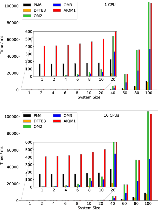
Figure 1: Runtime measurements with PM6, DFTB3, OM2, OM3, and AIQM1 implemented in SCINE Sparrow for linear alkanes of different sizes. The number given on the abscissa specifies the number of carbon atoms in the corresponding alkane. The top part depicts the runtime when utilizing a single processor core, the bottom part shows the runtimes when using 16 CPU cores.

AIQM1 shows an identical scaling behavior as OM2 and almost identical timings for the large systems. However, for small systems, namely methane to decane, the computation time for AIQM1 is significantly larger than that of any other method. What is more, for the systems up to hexane, this time is roughly constant, suggesting that for small systems, a constant (i.e., system size independent) effect dominates. This is most likely the initialization routine, combined with the fact that for some parts of the algorithm, external binaries are invoked (the spawning of a new process is rather time demanding). PM6 shows a similar, almost constant runtime for small systems up to decane, before increasing with a similar scaling like DFTB3. For the largest systems, PM6 needs only slightly more time than DFTB3.

It is interesting to investigate the effect of activating additional CPU cores when calculating the electronic energy. The most time-consuming parts of Sparrow are parallelized with OpenMP. However, the benefits of this parallelization are only expected to manifest themselves for very large systems, as for small systems, the overhead imposed by the parallelization adversely dominates the runtime: compare the top of Fig. 1 to its bottom part, which shows the same timings obtained on 16 CPU cores.

Up to icosane, all models require more time on 16 cores than on a single one. Starting with tetracontane, DFTB3 as well as PM6 show a slight speedup, whereas the other models still do not benefit from the additional CPU cores. However, as we have noted above, the current implementation of OM2, OM3, and AIQM1 have only very little parallelization, so this is expected. One must keep in mind that most modern CPUs do adjust their operating frequency depending on how many CPU cores are utilized. The Intel Xeon E5-2667 v2 processor chosen for this work features a maximum peak frequency of 4.00 GHz. This is the frequency we can expect to be in operation when Sparrow runs on a single CPU core. When all cores are utilized, however, the CPU is expected to throttle the frequency to 3.30 GHz, implying a performance drop of about 17.5 % for a single core. Therefore, the maximum speedup expected when utilizing all 16 cores — considering only the CPU frequency — is a factor of 13.2. Obviously, the speedup of a factor of only 1.17 as seen for DFTB3 is clearly below this theoretical threshold, implying that the current parallelization of Sparrow has ample room for improvement.

3.2 Speedup Attainable on Higher-Performance Hardware

It is instructive to investigate the effect different CPU models have on the calculation times. All timings reported in the previous section have been obtained on a machine with two Intel Xeon E5-2667 v2 processors. This old CPU type released in the second half of 2013 features a base frequency of 3.30 GHz and a maximum peak frequency of 4.00 GHz. For comparison, we repeated the timings on a more recent Intel Xeon W-1390P processor released in 2021, featuring a base frequency of 3.50 GHz and a maximum peak frequency of 5.30 GHz. Considering only the peak frequencies, one would expect any Sparrow calculation to run about 1.33 times faster on the more modern CPU.

A comparison of the runtimes of DFTB3 and AIQM1 for the series of linear alkanes studied is presented in Fig. 2. Here, all calculations were run on a single CPU core. As one can see, for all system sizes calculations with AIQM1 are significantly faster, namely about a factor of 1.8 for the smallest systems and a factor of roughly 1.6 for hectane. This is significantly larger than the theoretical speedup expected based on a comparison of the CPU frequencies alone. This highlights that a multitude of factors affect the calculation runtime besides the processor frequency, such as memory and disk speeds. For our test machine with the more modern CPU, also the rest of the hardware is newer and more performant compared to their counterparts in the older machine. For example, the main memory in the older machine runs at an internal clock frequency of 233 MHz, achieving a data transfer rate of about 15 GB/s. In the newer machine, the memory works at 400 MHz, and the total data transfer rate is almost 26 GB/s. All these factors combine for a significant total speedup.

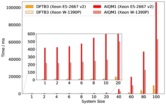
Figure 2: Runtimes of DFTB3 and AIQM1 models implemented in SCINE Sparrow for various linear alkanes on different CPU types.

While the runtimes of DFTB3 show a similar speedup for the large systems, most curiously, however, this speedup is reversed for the small systems. For methane and ethane, the total time needed to calculate the electronic energy is about a factor of three larger on the more modern computer. Without a more detailed drill-down analysis, it is difficult to unambiguously determine the cause for this reversal. Obviously, the CPU speed as the dominant factor for the computing time is the more important, the larger the systems are. For small systems, the overhead imposed by initialization routines takes a higher percentage of the total runtime than for large systems. During the initialization, Sparrow reads in parameters from disk, among other data. One may speculate that this reading from disk is, for some reason, slower on the newer machine compared to the older one.

3.3 Comparison to Different Computer Programs

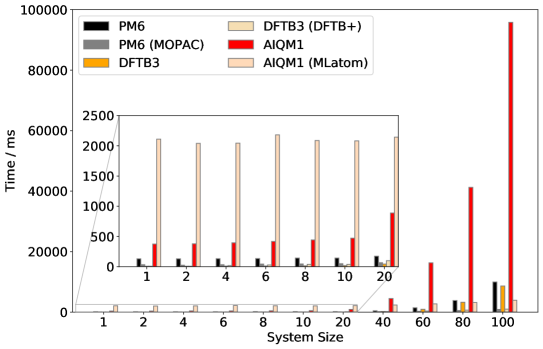
Figure 3: Comparison of runtimes of DFTB3, PM6, and AIQM1 models measured with SCINE Sparrow and compared to the corresponding implementations of MOPAC¹¹³, DFTB+⁷, and MLatom interfaced to the MNDO program, respectively, for various linear alkanes. The timings have been measured on a single core of an Intel Xeon Gold 5222 processor (to obtain these particular timings, Sparrow has been compiled with GCC 7.4.0, the Intel Math Kernel Library 2019.1.144, Eigen 3.3.9, and the Boost library 1.73.0).

A comparison of the runtime of Sparrow to that of other programs implementing the same methods is obviously of great interest. In Fig. 3, we present a runtime comparison of PM6, DFTB3 and AIQM1 as implemented in Sparrow, MOPAC 2016 (version 19.090L)¹¹³, DFTB+ 22.2⁷ and MLatom^{114, 115, 116} (interfaced to the MNDO program¹¹⁷ providing the ODM2* part, TorchANI providing the NN part and dftd4 providing the D4 part), respectively. Care has been taken to set numerical thresholds such that convergence settings were as similar as possible for the sake of comparability.

As one can see, the PM6 implementation in MOPAC is consistently faster than the one of Sparrow. Depending on the exact system studied, MOPAC is about a factor of 4 (tetracontane) to 10 (methane, hectane) faster than SCINE Sparrow. For DFTB3, Sparrow’s implementation is somewhat faster for the smaller systems (up to a factor of about 2 for methane) than that provided by DFTB+. However, starting with tetracontane, DFTB+ begins to be faster than Sparrow; for hectane, the implementation of DFTB+ is about a factor of 7 faster. For AIQM1, Sparrow’s implementation also somewhat faster for the smaller systems (up to a factor of about 5 for butane) than that provided by MLatom interfaced to the MNDO program. This is because the file reading and writing process is the most time-consuming part in MLatom for the smaller systems. For larger systems, where calculations of the ODM2* part with the MNDO program dominate, we find that MLatom’s AIQM1 calculations are much faster than by Sparrow, and even faster than PM6 and DFTB3 by Sparrow.

Despite being slower in some cases, we emphasize that the strong focus on interactive quantum chemistry of Sparrow has not only motivated the development of ways to reduce the computation time of a individual single point calculation (for which we reported the timings above), but also to accelerate an entire series of such calculations (see also section 3.5). Naturally, it can be expected that future developments are likely to also reduce the single-point timings.

3.4 Implications for High-Throughput Virtual Screening

We can relate the runtimes discussed above to high-throughput virtual screening as well as interactive quantum chemistry. For this purpose, we first define three different molecule sizes and the typical time required to calculate their ground state electronic energy with Sparrow, cf., Table 3.

Table 3: Typical runtimes required by different semi-empirical models of SCINE Sparrow for different molecule sizes. All times are given in ms.

Method	Small (butane-like)	Medium (icosane-like)	Large (hectane-like)
PM6	76	100	5300
DFTB3	6	30	4800
OM2	17	290	61800
OM3	13	180	26100
AIQM1	224	500	63100

For small, butane-like molecules, calculations typically need less than 100 ms with the exception of AIQM1. For molecules of medium size (comparable to icosane), runtimes vary between 30 and 500 ms, depending on the method chosen. Large, hectane-like molecules imply runtimes between about 5 s and one minute. With these runtimes, we can estimate the total amount of molecules one can screen within 10’000 CPU hours, amounting to a small-scale high-throughput virtual screening campaign employing 100 CPU cores for about 4 days (cf., Table 4).

Table 4: Total number of molecules which can be screened within 10’000 CPU hours by different semi-empirical methods implemented in SCINE Sparrow for different molecule sizes.

Method	Small (butane-like)	Medium (icosane-like)	Large (hectane-like)
PM6	473’684’210	360’000’000	6’792’452
DFTB3	6’000’000’000	1’200’000’000	7’500’000
OM2	2’117’647’058	124’137’931	582’524
OM3	2’769’230’769	200’000’000	1’379’310
AIQM1	160’714’285	72’000’000	570’522

As one can see, very efficient models such as PM6 and DFTB3 can screen several millions of large (hectane-like) molecules in this time frame, while the more involved methods OM2 and AIQM1 can screen more than 500’000 large molecules. For small systems, the throughput rate increases, reaching no fewer than 6 billion small, butane-like molecules with DFTB3 within only 10’000 CPU hours.

3.5 Implications for Interactive Quantum Chemistry

Interactive quantum mechanics places a different focus on automated high-throughput calculations: A maximum runtime must not be exceeded, which eventually limits the molecular size that can be studied. For interactive quantum chemistry, we have seen above that calculation times should not exceed about 34 ms for a fluent visual feedback, and for haptic feedback this limit is even lower (depending on additional tricks such as the mediator potential⁴¹). Comparing this to the runtimes reported above, we see that the maximum molecule size which can currently be treated interactively is between decane and icosane for the fastest method DFTB3 when only visual feedback is needed (allowing for up to 10 ms of latency, see above). However, we have to keep in mind that when a human person is interactively manipulating the atomic coordinates of a molecule, these change in a rather smooth, continuous way. The consequence is that successive structures occurring in an interactive quantum chemistry application are rather similar to each other. Consequently, this can be exploited to accelerate the calculations. In Sparrow, it is possible to use the density matrix of the previous calculation as the starting point for the next calculation¹⁰¹. If two structures are rather similar to one another, also their density matrices will be similar, making such a starting guess a good approximation. To showcase this, we demonstrate a series of calculations on a molecular trajectory representing a keto–enol tautomerism of a long-chained molecule. A few snapshots along this trajectory are presented in Fig. 4 (here, we employ the trajectory called “T1” from Ref. 118). When calculating all 200 frames of this trajectory with the DFTB3 method implemented in Sparrow independently of each other, the total runtime is 4944.6 ms. When re-using the density matrix of the previous structure, the runtime drops to 3434.3 ms, i.e., it is reduced by a factor of 1.4. This is roughly consistent with the decrease of the average number of SCF cycles needed, being 11.7 when the density matrix is not re-used and 7.5 otherwise. A similar speedup by a factor of 1.5 is also observed for the PM6 model. This increase in calculation rate directly translates into larger molecules being amenable to an interactive manipulation. In practice, molecules containing up to thirty heavy atoms are straightforward to deal with in an interactive setting on custom present-day hardware.

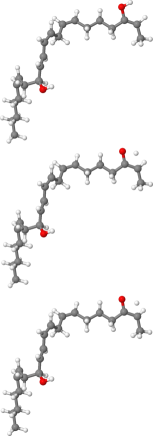
Figure 4: Three snapshots along a trajectory representing a keto–enol tautomerism of a long-chained molecule taken from trajectory T1 of Ref. 118. Note the similarity of all three structures.

We note that for OM3, the speedup observed when injecting the previous density matrix is only a factor of 1.07, even though also in this case, the average number of SCF cycles required for convergence is also reduced by about a factor of 1.5, namely from 14.8 to 10.1. This is evidence for two factors decreasing the computational efficiency of OM3. First, the total number of SCF cycles needed is higher for OM3 compared to DFTB3 or PM6. Second, for OM3, some part of the algorithm outside the SCF routine needs comparatively much time. Clearly, this indicates potential for future optimizations.

For a fluent haptic feedback, the runtimes reported in this work suggest that only very small molecules can be treated. Indeed, the high feedback frequency needed poses a problem also for very efficient semi-empirical methods on contemporary hardware. Therefore, besides a number of algorithmic improvements tailoring the methods in Sparrow to interactive quantum chemistry, also other completely complementary approaches have to be developed. Within the current SCINE framework, the most important of these is the so-called mediator potential, which is a surrogate function modelling essentially a harmonic potential to which the displacement of all atomic nuclei is subjected. The parameters of this potential are obtained from a calculation with Sparrow. Afterwards, this simple function can be evaluated extremely quickly, and restrains the interactive manipulation to the region of the potential energy surface for which a calculation with Sparrow has already been carried out. In the background, semi-empirical calculations are continuously carried out such that the surrogate function can be continuously updated, enabling a fluent manipulation of the system. We refer the interested reader to Ref. 41 for more details on this approach.

4 Conclusions and Outlook

In this work, we presented the open-source free-of-charge SCINE Sparrow (https://github.com/qcscine/sparrow), a C++ program implementing a wide range of semi-empirical electronic structure models. We reported a new implementation of the orthogonalization-corrected methods OM2 and OM3 as well as AIQM1, which is an artificial intelligence-enhanced approach based on the OMx model. We discussed key design principles of Sparrow, highlighting how it is especially tailored towards applications in interactive quantum chemistry.

SCINE Sparrow offers a unique collection of semi-empirical approaches broadly ranging from traditional MNDO-type to more advanced orthogonalization-corrected to DFTB-type to state-of-the-art machine learning-improved AIQM1 methods. Sparrow is used as backend with MLatom^{115, 116} to enable AIQM1 calculations that can be performed on the MLatom@XACS cloud¹¹⁹ in a web browser without the need for any software installation, further increasing the accessibility of quantum chemistry.

We then reported the runtimes of a range of semi-empirical models currently implemented in Sparrow for molecules of different sizes, demonstrating the suitability of semi-empirical methods in general as well as their implementation in Sparrow for high-throughput virtual screening, ab initio molecular dynamics simulations, as well as interactive quantum chemistry. For screening purposes, semi-empirical methods allow one to screen a huge number of molecules with only modest computational resources. For interactive applications, semi-empirical methods are currently the only way to simulate molecular systems quantum mechanically and on the fly, i.e., without precomputing the potential energy surface.

The runtimes presented in this work also highlight potential directions for the further improvement of Sparrow. For example, the newly implemented methods OM2, OM3, and AIQM1 show a very steep scaling with molecule size. While the time needed by OM2 and OM3 for small molecules is among the shortest of all methods implemented in Sparrow, these methods are about an order of magnitude larger compared to PM6 or DFTB3 for large systems. However, we note that further improvement of the software may increase the efficiency of thee new approaches by an order of magnitude. Furthermore, analytical nuclear gradients are currently not available for OM2, OM3 and AIQM1 in Sparrow. Future work in Sparrow will address these points.

Author Declaration

The authors have no conflict of interest to declare.

Data Availability Statement

The data that support the findings of this study are available from the corresponding author upon request.

Appendix: Running SCINE Sparrow

Sparrow can be used either as a standalone binary via the command line or as a library via C++ or Python. When used as a standalone binary, the command

sparrow -h

provides a list of all available options. For example, a simple calculation of the electronic energy of a structure in the file structure.xyz with the MNDO method can be achieved with

sparrow -x structure.xyz -M MNDO

By default, a spin multiplicity of 1 and a charge of 0 are assumed; the calculation is carried out in the spin-restricted formalism. Suppose we want to specify a charge of +1 and a spin multiplicity of 2. For this case, the following options have to be specified:

sparrow -x structure.xyz -M MNDO -c 1 -s 2

The following example calculates the nuclear gradients as well as the Hessian matrix with the AM1 method:

sparrow -x structure.xyz -M AM1 -G -H

The following code snippet illustrates the usage of Sparrow via Python; here the electronic energy as well as the nuclear gradients are calculated with the OM3 method:

import scine_utilities as su
import scine_sparrow

manager = su.core.ModuleManager()
calculator = manager.get(’calculator’, ’OM3’)
calculator.structure = su.io.read(’structure.xyz’)[0]
calculator.set_required_properties([su.Property.Energy, su.Property.Gradients])

results = calculator.calculate()
print(results.energy)
print(results.gradients)

Further examples and instructions concerning the usage of Sparrow are given in the manual, provided together with the source code of Sparrow^{54, 112}.

References

- Hennemann and Clark 2014 Hennemann, M.; Clark, T. EMPIRE: a highly parallel semiempirical molecular orbital program: 1: self-consistent field calculations. J. Mol. Model. 2014, 20, 2331
- Dral 2014 Dral, P. O. The unrestricted local properties: application in nanoelectronics and for predicting radicals reactivity. J. Mol. Model. 2014, 20, 2134
- Wu et al. 2012 Wu, X.; Koslowski, A.; Thiel, W. Semiempirical Quantum Chemical Calculations Accelerated on a Hybrid Multicore CPU-GPU Computing Platform. J. Chem. Theory Comput. 2012, 8, 2272–2281
- Maia et al. 2012 Maia, J. D. C; Urquiza Carvalho, G. A.; Mangueira, Jr., C. P.; Santana, S. R.; Cabral, L. A. F.; Rocha, G. B. GPU Linear Algebra Libraries and GPGPU Programming for Accelerating MOPAC Semiempirical Quantum Chemistry Calculations. J. Chem. Theory Comput. 2012, 8, 3072–3081
- Zhou et al. 2020 Zhou, G.; Nebgen, B.; Lubbers, N.; Malone, W. F.; Niklasson, A. M. N.; Tretiak, S. Graphics Processing Unit-Accelerated Semiempirical Born Oppenheimer Molecular Dynamics Using PyTorch. J. Chem. Theory Comput. 2020, 16, 4951–4962
- Stewart 2008 Stewart, J. J. P. Application of the PM6 method to modeling proteins. J. Mol. Model. 2008, 15, 765–805
- Hourahine et al. 2020 Hourahine, B. et al. DFTB+, a software package for efficient approximate density functional theory based atomistic simulations. J. Chem. Phys. 2020, 152, 124101
- Shoichet 2004 Shoichet, B. K. Virtual screening of chemical libraries. Nature 2004, 432, 862–865
- Pyzer-Knapp et al. 2015 Pyzer-Knapp, E. O.; Suh, C.; Gómez-Bombarelli, R.; Aguilera-Iparraguirre, J.; Aspuru-Guzik, A. What Is High-Throughput Virtual Screening? A Perspective from Organic Materials Discovery. Annu. Rev. Mater. Res. 2015, 45, 195–216
- Halls and Tasaki 2010 Halls, M. D.; Tasaki, K. High-throughput quantum chemistry and virtual screening for lithium ion battery electrolyte additives. J. Power Sources 2010, 195, 1472–1478
- Kromann et al. 2016 Kromann, J. C.; Larsen, F.; Moustafa, H.; Jensen, J. H. Prediction of pKa values using the PM6 semiempirical method. PeerJ 2016, 4, e2335
- Wilbraham et al. 2018 Wilbraham, L.; Berardo, E.; Turcani, L.; Jelfs, K. E.; Zwijnenburg, M. A. High-Throughput Screening Approach for the Optoelectronic Properties of Conjugated Polymers. J. Chem. Inf. Model. 2018, 58, 2450–2459
- Heath-Apostolopoulos et al. 2019 Heath-Apostolopoulos, I.; Wilbraham, L.; A. Zwijnenburg, M. Computational high-throughput screening of polymeric photocatalysts: exploring the effect of composition, sequence isomerism and conformational degrees of freedom. Faraday Discuss. 2019, 215, 98–110
- Wen et al. 2022 Wen, L.; Wang, B.; Yu, T.; Lai, W.; Shi, J.; Liu, M.; Liu, Y. Accelerating the search of CHONF-containing highly energetic materials by combinatorial library design and high-throughput screening. Fuel 2022, 310, 122241
- Hachmann et al. 2011 Hachmann, J.; Olivares-Amaya, R.; Atahan-Evrenk, S.; Amador-Bedolla, C.; Sánchez-Carrera, R. S.; Gold-Parker, A.; Vogt, L.; Brockway, A. M.; Aspuru-Guzik, A. The Harvard Clean Energy Project: Large-Scale Computational Screening and Design of Organic Photovoltaics on the World Community Grid. J. Phys. Chem. Lett. 2011, 2, 2241–2251
- Kanal et al. 2013 Kanal, I. Y.; Owens, S. G.; Bechtel, J. S.; Hutchison, G. R. Efficient Computational Screening of Organic Polymer Photovoltaics. J. Phys. Chem. Lett. 2013, 4, 1613–1623
- Korth 2014 Korth, M. Large-scale virtual high-throughput screening for the identification of new battery electrolyte solvents: evaluation of electronic structure theory methods. Phys. Chem. Chem. Phys. 2014, 16, 7919–7926
- Martin et al. 2014 Martin, R. L.; Simon, C. M.; Smit, B.; Haranczyk, M. In silico Design of Porous Polymer Networks: High-Throughput Screening for Methane Storage Materials. J. Am. Chem. Soc. 2014, 136, 5006–5022
- Cheng et al. 2015 Cheng, L.; Assary, R. S.; Qu, X.; Jain, A.; Ong, S. P.; Rajput, N. N.; Persson, K.; Curtiss, L. A. Accelerating Electrolyte Discovery for Energy Storage with High-Throughput Screening. J. Phys. Chem. Lett. 2015, 6, 283–291
- Imamura et al. 2017 Imamura, Y.; Tashiro, M.; Katouda, M.; Hada, M. Automatic High-Throughput Screening Scheme for Organic Photovoltaics: Estimating the Orbital Energies of Polymers from Oligomers and Evaluating the Photovoltaic Characteristics. J. Phys. Chem. C 2017, 121, 28275–28286
- Schwöbel et al. 2017 Schwöbel, J. A. H.; Preißinger, M.; Brüggemann, D.; Klamt, A. High-Throughput Screening of Working Fluids for the Organic Rankine Cycle (ORC) Based on Conductor-like Screening Model for Realistic Solvation (COSMO-RS) and Thermodynamic Process Simulations. Ind. Eng. Chem. Res. 2017, 56, 788–798
- Irfan et al. 2022 Irfan, A.; Hussien, M.; Mehboob, M. Y.; Ahmad, A.; Janjua, M. R. S. A. Learning from Fullerenes and Predicting for Y6: Machine Learning and High-Throughput Screening of Small Molecule Donors for Organic Solar Cells. Energy Technol. 2022, 10, 2101096
- Ramakrishnan et al. 2014 Ramakrishnan, R.; Dral, P. O.; Rupp, M.; von Lilienfeld, O. A. Quantum chemistry structures and properties of 134 kilo molecules. Sci. Data 2014, 1, 140022
- Nakata et al. 2020 Nakata, M.; Shimazaki, T.; Hashimoto, M.; Maeda, T. PubChemQC PM6: Data Sets of 221 Million Molecules with Optimized Molecular Geometries and Electronic Properties. J. Chem. Inf. Model. 2020, 60, 5891–5899
- Ramakrishnan et al. 2015 Ramakrishnan, R.; Dral, P. O.; Rupp, M.; von Lilienfeld, O. A. Big Data Meets Quantum Chemistry Approximations: The -Machine Learning Approach. J. Chem. Theory Comput. 2015, 11, 2087–2096
- Li et al. 2018 Li, H.; Collins, C.; Tanha, M.; Gordon, G. J.; Yaron, D. J. A Density Functional Tight Binding Layer for Deep Learning of Chemical Hamiltonians. J. Chem. Theory Comput. 2018, 14, 5764–5776
- Christensen et al. 2021 Christensen, A. S.; Sirumalla, S. K.; Qiao, Z.; O’Connor, M. B.; Smith, D. G. A.; Ding, F.; Bygrave, P. J.; Anandkumar, A.; Welborn, M.; Manby, F. R.; Miller III, T. F. OrbNet Denali: A machine learning potential for biological and organic chemistry with semi-empirical cost and DFT accuracy. J. Chem. Phys. 2021, 155, 204103
- Fan et al. 2022 Fan, G.; McSloy, A.; Aradi, B.; Yam, C. Y.; Frauenheim, T. Obtaining Electronic Properties of Molecules through Combining Density Functional Tight Binding with Machine Learning. J. Phys. Chem. Lett. 2022, 10132–10139
- Jacobson et al. 2022 Jacobson, L. D.; Stevenson, J. M.; Ramezanghorbani, F.; Ghoreishi, D.; Leswing, K.; Harder, E. D.; Abel, R. Transferable Neural Network Potential Energy Surfaces for Closed-Shell Organic Molecules: Extension to Ions. J. Chem. Theory Comput. 2022, 18, 2354–2366
- Atz et al. 2022 Atz, K.; Isert, C.; Böcker, M. N. A.; Jiménez-Luna, J.; Schneider, G. -Quantum machine-learning for medicinal chemistry. Phys. Chem. Chem. Phys. 2022, 24, 10775–10783
- Zhou et al. 2022 Zhou, G.; Lubbers, N.; Barros, K.; Tretiak, S.; Nebgen, B. Deep learning of dynamically responsive chemical Hamiltonians with semiempirical quantum mechanics. Proc. Natl. Acad. Sci. U. S. A. 2022, 119, e2120333119
- Dral et al. 2015 Dral, P. O.; von Lilienfeld, O. A.; Thiel, W. Machine Learning of Parameters for Accurate Semiempirical Quantum Chemical Calculations. J. Chem. Theory Comput. 2015, 11, 2120–2125
- Zheng et al. 2021 Zheng, P.; Zubatyuk, R.; Wu, W.; Isayev, O.; Dral, P. O. Artificial intelligence-enhanced quantum chemical method with broad applicability. Nat. Commun. 2021, 12, 7022
- Dral and Zubatiuk 2023 Dral, P. O.; Zubatiuk, T. In Quantum Chemistry in the Age of Machine Learning; Dral, P. O., Ed.; Elsevier: Amsterdam, Netherlands, 2023
- Zheng et al. 2022 Zheng, P.; Yang, W.; Wu, W.; Isayev, O.; Dral, P. O. Toward Chemical Accuracy in Predicting Enthalpies of Formation with General-Purpose Data-Driven Methods. J. Phys. Chem. Lett. 2022, 13, 3479–3491
- Haag and Reiher 2013 Haag, M. P.; Reiher, M. Real-Time Quantum Chemistry. Int. J. Quantum Chem. 2013, 113, 8–20
- Haag and Reiher 2014 Haag, M. P.; Reiher, M. Studying chemical reactivity in a virtual environment. Faraday Discuss. 2014, 169, 89–118
- Haag et al. 2014 Haag, M. P.; Vaucher, A. C.; Bosson, M.; Redon, S.; Reiher, M. Interactive Chemical Reactivity Exploration. ChemPhysChem 2014, 15, 3301–3319
- Weymuth and Reiher 2021 Weymuth, T.; Reiher, M. Immersive Interactive Quantum Mechanics for Teaching and Learning Chemistry. Chimia 2021, 75, 45–49
- Marti and Reiher 2009 Marti, K. H.; Reiher, M. Haptic Quantum Chemistry. J. Comput. Chem. 2009, 30, 2010–2020
- Vaucher et al. 2016 Vaucher, A. C.; Haag, M. P.; Reiher, M. Real-Time Feedback from Iterative Electronic Structure Calculations. J. Comp. Chem. 2016, 37, 805–812
- Meuwly 2019 Meuwly, M. Reactive Molecular Dynamics: From Small Molecules to Proteins. WIREs Comput. Mol. Sci. 2019, 9, e1386
- Ochsenfeld et al. 2007 Ochsenfeld, C.; Kussmann, J.; Lambrecht, D. S. Reviews in Computational Chemistry; John Wiley & Sons, Inc.: Hoboken, New Jersey, USA, 2007; Vol. 23; pp 1–82
- Zaleśny et al. 2011 Zaleśny, R., Papadopoulos, M. G., Mezey, P. G., Leszczynski, J., Eds. Linear-Scaling Techniques in Computational Chemistry and Physics: Methods and Applications; Challenges and Advances in Computational Chemistry and Physics; Springer: Dordrecht, Netherlands, 2011; Vol. 13
- Bowler and Miyazaki 2012 Bowler, D. R.; Miyazaki, T. $\mathcal{O}(n)$ methods in electronic structure calculations. Rep. Prog. Phys. 2012, 75, 036503
- Mohr et al. 2015 Mohr, S.; Ratcliff, L. E.; Genovese, L.; Caliste, D.; Boulanger, P.; Goedecker, S.; Deutsch, T. Accurate and efficient linear scaling DFT calculations with universal applicability. Phys. Chem. Chem. Phys. 2015, 17, 31360–31370
- Kolb and Thiel 1993 Kolb, M.; Thiel, W. Beyond the MNDO model: Methodical considerations and numerical results. J. Comp. Chem. 1993, 14, 775–789
- Kolb 1991 Kolb, M. Ein neues semiempirisches Verfahren auf Grundlage der NDDO-Näherung: Entwicklung der Methode, Parametrisierung und Anwendung. Ph.D. thesis, 1991
- Weber and Thiel 2000 Weber, W.; Thiel, W. Orthogonalization corrections for semiempirical methods. Theor. Chem. Acc. 2000, 103, 495–506
- Weber 1996 Weber, W. Ein neues semiempirisches NDDO-Verfahren mit Orthogonalisierungskorrekturen: Entwicklung des Modells, Implementierung, Parametrisierung und Anwendung. Ph.D. thesis, 1996
- Scholten 2003 Scholten, M. Semiempirische Verfahren mit Orthogonalisierungskorrekturen: Die OM3 Methode. Ph.D. thesis, 2003
- Dral et al. 2016 Dral, P. O.; Wu, X.; Spörkel, L.; Koslowski, A.; Weber, W.; Steiger, R.; Scholten, M.; Thiel, W. Semiempirical Quantum-Chemical Orthogonalization-Corrected Methods: Theory, Implementation, and Parameters. J. Chem. Theory Comput. 2016, 12, 1082–1096
- Dral et al. 2019 Dral, P. O.; Wu, X.; Thiel, W. Semiempirical Quantum-Chemical Methods with Orthogonalization and Dispersion Corrections. J. Chem. Theory Comput. 2019, 15, 1743–1760
- Bosia et al. 2022 Bosia, F.; Husch, T.; Müller, C. H.; Polonius, S.; Sobez, J.-G.; Steiner, M.; Unsleber, J. P.; Vaucher, A. C.; Weymuth, T.; Reiher, M. SCINE Sparrow: Release 3.1.0. 2022
- Husch et al. 2018 Husch, T.; Vaucher, A. C.; Reiher, M. Semiempirical molecular orbital models based on the neglect of diatomic differential overlap approximation. Int. J. Quantum Chem. 2018, 118, e25799
- Dral and Řezáč 2023 Dral, P. O.; Řezáč, J. In Quantum Chemistry in the Age of Machine Learning; Dral, P. O., Ed.; Elsevier: Amsterdam, Netherlands, 2023
- Porezag et al. 1995 Porezag, D.; Frauenheim, T.; Köhler, T.; Seifert, G.; Kaschner, R. Construction of Tight-Binding-like Potentials on the Basis of Density-Functional Theory: Application to Carbon. Phys. Rev. B 1995, 51, 12947–12957
- Seifert et al. 1996 Seifert, G.; Porezag, D.; Frauenheim, T. Calculations of Molecules, Clusters, and Solids with a Simplified LCAO-DFT-LDA Scheme. Int. J. Quantum Chem. 1996, 58, 185–192
- Elstner et al. 1998 Elstner, M.; Porezag, D.; Jungnickel, G.; Elsner, J.; Haugk, M.; Frauenheim, T.; Suhai, S.; Seifert, G. Self-Consistent-Charge Density-Functional Tight-Binding Method for Simulations of Complex Materials Properties. Phys. Rev. B 1998, 58, 7260–7268
- Gaus et al. 2011 Gaus, M.; Cui, Q.; Elstner, M. DFTB3: Extension of the Self-Consistent-Charge Density-Functional Tight-Binding Method (SCC-DFTB). J. Chem. Theory Comput. 2011, 7, 931–948
- Dewar and Thiel 1977 Dewar, M. J. S.; Thiel, W. Ground states of molecules. 38. The MNDO method. Approximations and parameters. J. Am. Chem. Soc. 1977, 99, 4899–4907
- Thiel and Voityuk 1992 Thiel, W.; Voityuk, A. A. Extension of the MNDO formalism to d orbitals: Integral approximations and preliminary numerical results. Theor. Chim. Acta 1992, 81, 391–404
- Dewar et al. 1985 Dewar, M. J. S.; Zoebisch, E. G.; Healy, E. F.; Stewart, J. J. P. Development and use of quantum mechanical molecular models. 76. AM1: a new general purpose quantum mechanical molecular model. J. Am. Chem. Soc. 1985, 107, 3902–3909
- Rocha et al. 2006 Rocha, G. B.; Freire, R. O.; Simas, A. M.; Stewart, J. J. P. RM1: A reparameterization of AM1 for H, C, N, O, P, S, F, Cl, Br, and I. J. Comput. Chem. 2006, 27, 1101–1111
- Stewart 1989 Stewart, J. J. P. Optimization of parameters for semiempirical methods I. Method. J. Comput. Chem. 1989, 10, 209–220
- Stewart 1989 Stewart, J. J. P. Optimization of parameters for semiempirical methods II. Applications. J. Comput. Chem. 1989, 10, 221–264
- Stewart 2007 Stewart, J. J. P. Optimization of parameters for semiempirical methods V: Modification of NDDO approximations and application to 70 elements. J. Mol. Model. 2007, 13, 1173–1213
- Stewart 2013 Stewart, J. J. P. Optimization of parameters for semiempirical methods VI: more modifications to the NDDO approximations and re-optimization of parameters. J. Mol. Model. 2013, 19, 1–32
- Vaucher 2018 Vaucher, A. C. Interactive Control of Quantum Mechanical Calculations in Chemistry. Ph.D. thesis, ETH Zurich, Zurich, 2018
- Řezáč et al. 2009 Řezáč, J.; Fanfrlík, J.; Salahub, D.; Hobza, P. Semiempirical Quantum Chemical PM6 Method Augmented by Dispersion and H-Bonding Correction Terms Reliably Describes Various Types of Noncovalent Complexes. J. Chem. Theory Comput. 2009, 5, 1749–1760
- Korth et al. 2010 Korth, M.; Pitoňák, M.; Řezáč, J.; Hobza, P. A Transferable H-Bonding Correction for Semiempirical Quantum-Chemical Methods. J. Chem. Theory Comput. 2010, 6, 344–352
- Korth 2010 Korth, M. Third-Generation Hydrogen-Bonding Corrections for Semiempirical QM Methods and Force Fields. J. Chem. Theory Comput. 2010, 6, 3808–3816
- Řezáč and Hobza 2012 Řezáč, J.; Hobza, P. Advanced Corrections of Hydrogen Bonding and Dispersion for Semiempirical Quantum Mechanical Methods. J. Chem. Theory Comput. 2012, 8, 141–151
- Elstner and Seifert 2014 Elstner, M.; Seifert, G. Density Functional Tight Binding. Phil.Trans. R. Soc. A 2014, 372, 20120483
- Pracht et al. 2019 Pracht, P.; Caldeweyher, E.; Ehlert, S.; Grimme, S. A Robust Non-Self-Consistent Tight-Binding Quantum Chemistry Method for Large Molecules. 2019
- Grimme et al. 2017 Grimme, S.; Bannwarth, C.; Shushkov, P. A Robust and Accurate Tight-Binding Quantum Chemical Method for Structures, Vibrational Frequencies, and Noncovalent Interactions of Large Molecular Systems Parametrized for All spd-Block Elements (Z = 1–86). J. Chem. Theory Comput. 2017, 13, 1989–2009
- Bannwarth et al. 2019 Bannwarth, C.; Ehlert, S.; Grimme, S. GFN2-xTB—An Accurate and Broadly Parametrized Self-Consistent Tight-Binding Quantum Chemical Method with Multipole Electrostatics and Density-Dependent Dispersion Contributions. J. Chem. Theory Comput. 2019, 15, 1652–1671
- 78 https://evaleev.github.io/libint (accessed November 17, 2022)
- Löwdin 1950 Löwdin, P.-O. On the Non‐Orthogonality Problem Connected with the Use of Atomic Wave Functions in the Theory of Molecules and Crystals. J. Chem. Phys. 1950, 18, 365–375
- Wu et al. 2019 Wu, X.; Dral, P. O.; Koslowski, A.; Thiel, W. Big data analysis of ab Initio molecular integrals in the neglect of diatomic differential overlap approximation. J. Comput. Chem. 2019, 40, 638–649
- Grimme et al. 2010 Grimme, S.; Antony, J.; Ehrlich, S.; Krieg, H. A consistent and accurate ab initio parametrization of density functional dispersion correction (DFT-D) for the 94 elements H-Pu. J. Chem. Phys. 2010, 132, 154104
- Mohr et al. 2016 Mohr, P. J.; Newell, D. B.; Taylor, B. N. CODATA recommended values of the fundamental physical constants: 2014. Rev. Mod. Phys. 2016, 88, 035009
- Smith et al. 2017 Smith, J. S.; Isayev, O.; Roitberg, A. E. ANI-1: an extensible neural network potential with DFT accuracy at force field computational cost. Chem. Sci. 2017, 8, 3192–3203
- Smith et al. 2019 Smith, J. S.; Nebgen, B. T.; Zubatyuk, R.; Lubbers, N.; Devereux, C.; Barros, K.; Tretiak, S.; Isayev, O.; Roitberg, A. E. Approaching coupled cluster accuracy with a general-purpose neural network potential through transfer learning. Nat. Commun. 2019, 10, 8
- Devereux et al. 2020 Devereux, C.; Smith, J. S.; Davis, K. K.; Barros, K.; Zubatyuk, R.; Isayev, O.; Roitberg, A. E. Extending the Applicability of the ANI Deep Learning Molecular Potential to Sulfur and Halogens. J. Chem. Theory Comput. 2020, 16, 4192–4202
- Caldeweyher et al. 2017 Caldeweyher, E.; Bannwarth, C.; Grimme, S. Extension of the D3 dispersion coefficient model. J. Chem. Phys. 2017, 147, 034112
- Caldeweyher et al. 2019 Caldeweyher, E.; Ehlert, S.; Hansen, A.; Neugebauer, H.; Spicher, S.; Bannwarth, C.; Grimme, S. A generally applicable atomic-charge dependent London dispersion correction. J. Chem. Phys. 2019, 150, 19
- Behler and Parrinello 2007 Behler, J.; Parrinello, M. Generalized neural-network representation of high-dimensional potential-energy surfaces. Phys. Rev. Lett. 2007, 98, 4
- Gao et al. 2020 Gao, X.; Ramezanghorbani, F.; Isayev, O.; Smith, J. S.; Roitberg, A. E. TorchANI: A Free and Open Source PyTorch-Based Deep Learning Implementation of the ANI Neural Network Potentials. J. Chem. Inf. Model. 2020, 60, 3408–3415
- Smith et al. 2018 Smith, J. S.; Nebgen, B.; Lubbers, N.; Isayev, O.; Roitberg, A. E. Less is more: Sampling chemical space with active learning. J. Chem. Phys. 2018, 148, 241733
- Grimme et al. 2011 Grimme, S.; Ehrlich, S.; Goerigk, L. Effect of the Damping Function in Dispersion Corrected Density Functional Theory. J. Comp. Chem. 2011, 32, 1456–1465
- Caldeweyher et al. 2022 Caldeweyher, E.; Ehlert, S.; Grimme, S. DFT-D4 version 3.4.0. 2022
- Saunders and Hillier 1973 Saunders, V. R.; Hillier, I. H. A “Level-Shifting” Method for Converging Closed Shell Hartree-Fock Wave Functions. Int. J. Quantum Chem. 1973, 7, 699–705
- Pulay 1980 Pulay, P. Convergence acceleration of iterative sequences. The case of SCF iteration. Chem Phys Lett 1980, 73, 393–398
- Pulay 1982 Pulay, P. Improved SCF Convergence Acceleration. J. Comput. Chem. 1982, 3, 556–560
- Kudin et al. 2002 Kudin, K. N.; Scuseria, G. E.; Cancès, E. A black-box self-consistent field convergence algorithm: One step closer. J. Chem. Phys. 2002, 116, 8255–8261
- Høst et al. 2008 Høst, S.; Olsen, J.; Jansík, B.; Thøgersen, L.; Jørgensen, P.; Helgaker, T. The augmented Roothaan–Hall method for optimizing Hartree–Fock and Kohn–Sham density matrices. J. Chem. Phys. 2008, 129, 124106
- Hu and Yang 2010 Hu, X.; Yang, W. Accelerating self-consistent field convergence with the augmented Roothaan–Hall energy function. J. Chem. Phys. 2010, 132, 054109
- Chen and Wang 2011 Chen, Y. K.; Wang, Y. A. LISTb: a Better Direct Approach to LIST. J. Chem. Theory Comput. 2011, 7, 3045–3048
- Wang et al. 2011 Wang, Y. A.; Yam, C. Y.; Chen, Y. K.; Chen, G. Communication: Linear-expansion shooting techniques for accelerating self-consistent field convergence. J. Chem. Phys. 2011, 134, 241103
- Mühlbach et al. 2016 Mühlbach, A. H.; Vaucher, A. C.; Reiher, M. Accelerating Wave Function Convergence in Interactive Quantum Chemical Reactivity Studies. J. Chem. Theory Comput. 2016, 12, 1228–1235
- Atsumi and Nakai 2010 Atsumi, T.; Nakai, H. Acceleration of self-consistent-field convergence in ab initio molecular dynamics and Monte Carlo simulations and geometry optimization. Chem. Phys. Lett. 2010, 490, 102–108
- Almlöf et al. 1982 Almlöf, J.; Faegri Jr., K.; Korsell, K. Principles for a Direct scf Approach to lcao–mo Ab-Initio Calculations. J. Comput. Chem. 1982, 3, 385–399
- Cremer and Gauss 1986 Cremer, D.; Gauss, J. An Unconventional SCF Method for Calculations on Large Molecules. J. Comput. Chem. 1986, 7, 274–282
- Häser and Ahlrichs 1989 Häser, M.; Ahlrichs, R. Improvements on the Direct SCF Method. J. Comput. Chem. 1989, 10, 104–111
- Brunken et al. 2022 Brunken, C.; Csizi, K.-S.; Grimmel, S. A.; Gugler, S.; Sobez, J.-G.; Steiner, M.; Türtscher, P. L.; Unsleber, J. P.; Vaucher, A. C.; Weymuth, T.; Reiher, M. SCINE ReaDuct: Release 4.1.0. 2022
- Vaucher and Reiher 2016 Vaucher, A. C.; Reiher, M. Molecular Propensity as a Driver for Explorative Reactivity Studies. J. Chem. Inf. Model. 2016, 56, 1470–1478
- 108 https://gcc.gnu.org/ (accessed November 17, 2022)
- 109 https://www.intel.com/content/www/us/en/developer/tools/oneapi/onemkl.html (accessed November 17, 2022)
- 110 https://eigen.tuxfamily.org/index.php (accessed November 17, 2022)
- 111 https://www.boost.org/ (accessed November 17, 2022)
- Bosia et al. 2022 Bosia, F.; Husch, T.; Müller, C. H.; Polonius, S.; Sobez, J.-G.; Steiner, M.; Unsleber, J. P.; Vaucher, A. C.; Weymuth, T.; Zheng, P.; Reiher, M. SCINE Sparrow: Development Version 7b41c57. 2022
- 113 Stewart, J. P. P. Mopac 2016, version 19.090L, Stewart Computational Chemistry, Colorado Springs, CO, USA, http://OpenMOPAC.net (accessed Jauary 10, 2023)
- Dral et al. 2013–2023 Dral, P. O.; Zheng, P.; Xue, B.-X.; Ge, F.; Hou, Y.-F.; Pinheiro, Jr., M.; Su, Y.; Dai, Y.; Chen, Y. MLatom: a Package for Atomistic Simulations with Machine Learning, development version. http://MLatom.com (accessed on January 10, 2023). Xiamen University: Xiamen 361005, China, 2013–2023
- Dral 2019 Dral, P. O. MLatom: A Program Package for Quantum Chemical Research Assisted by Machine Learning. J. Comput. Chem. 2019, 40, 2339–2347
- Dral et al. 2021 Dral, P. O.; Ge, F.; Xue, B.-X.; Hou, Y.-F.; Pinheiro Jr., M.; Huang, J.; Barbatti, M. MLatom 2: An Integrative Platform for Atomistic Machine Learning. Top. Curr. Chem. 2021, 379, 27, http://MLatom.com, accessed: 2022-11-18
- Thiel 2020 Thiel, W. with contributions from M. Beck, S. Billeter, R. Kevorkiants, M. Kolb, A. Koslowski, S. Patchkovskii, A. Turner, E.-U. Wallenborn, W. Weber, L. Spörkel, and P. O. Dral. MNDO2020: a semiempirical quantum chemistry program. https://mndo.kofo.mpg.de (accessed on January 10, 2023). 2020
- Bosia et al. 2022 Bosia, F.; Weymuth, T.; Reiher, M. Ultra-fast spectroscopy for high-throughput and interactive quantum chemistry. Int. J. Quantum Chem. 2022, 122, e26966
- 119 Xiamen Atomistic Computing Suite (XACS) cloud computing service. http://XACScloud.com, accessed: 2022-11-18