Discontinuous Galerkin method for linear wave equations involving derivatives of the Dirac delta distribution

Abstract

Linear wave equations sourced by a Dirac delta distribution $\delta(x)$ and its derivative(s) can serve as a model for many different phenomena. We describe a discontinuous Galerkin (DG) method to numerically solve such equations with source terms proportional to $\partial^{n}\delta/\partial x^{n}$. Despite the presence of singular source terms, which imply discontinuous or potentially singular solutions, our DG method achieves global spectral accuracy even at the source’s location. Our DG method is developed for the wave equation written in fully first-order form. The first-order reduction is carried out using a distributional auxiliary variable that removes some of the source term’s singular behavior. While this is helpful numerically, it gives rise to a distributional constraint. We show that a time-independent spurious solution can develop if the initial constraint violation is proportional to $\delta(x)$. Numerical experiments verify this behavior and our scheme’s convergence properties by comparing against exact solutions.

1 Introduction

In this article we describe a discontinuous Galerkin (DG) method Reed.W;Hill.T1973 ; Hesthaven2008 ; Cock01 ; cockburn1998runge ; Cockburn.B1998 ; Cockburn.B;Karniadakis.G;Shu.C2000 for solving the wave equation

$$-\partial_{t}^{2}\psi+\partial_{x}^{2}\psi+V(x)\psi=\sum_{n=0}^{N}a_{n}(t,x)\delta^{(n)}(x)\,,$$ (1)

where $x\in[a,b]$, $V$ is a potential, $\delta^{(n)}(x)=\partial_{x}^{n}\delta(x)$ is the $n^{\rm th}$ distributional derivative friedlander1998introduction of a Dirac delta distribution $\delta(x)$, and $a_{n}(t,x)$ are arbitrary (classical) functions. We let the functions $\psi_{0}(x)=\psi(0,x)$ and $\dot{\psi}_{0}(x)=\partial_{t}\psi(0,x)$ specify the initial data. Differential equations of the form (1) arise when modeling phenomena driven by well-localized sources and have found applications as diverse as neuroscience casti2002population ; caceres2011analysis , seismology petersson2009stable ; shearer2019introduction , and gravitational wave physics sundararajan2007towards ; poisson2011motion . As one example, when a rotating blackhole is perturbed by a small, compact object the relevant (Teukolsky) equation features terms proportional to $\delta^{(2)}(x)$ on the right-hand-side sundararajan2007towards . To solve Eq. (1), various “regularized” numerical approaches engquist2005discretization ; tornberg2004numerical and schemes sundararajan2007towards ; sundararajan2008towards ; field2021gpu ; canizares2010pseudospectral ; canizares2009simulations ; jung2007spectral ; lousto2005time ; sopuerta2006finite have been proposed. Most of these methods only treat source terms proportional to $\delta(x)$ and $\delta^{(1)}(x)$ and do not achieve spectral accuracy at $x=0$.

Discontinuous Galerkin methods are especially well suited for solving Eq. (1) and, more broadly, problems with delta distributions. Indeed, the solution’s non-smoothness can be “hidden” at an interface between subdomains. Furthermore, the DG method solves the weak form of the problem, a natural setting for the delta distribution.

To the best of our knowledge, two distinct DG-based strategies have appeared in the literature for solving hyperbolic equations with $\delta$-singularities. Yang and Shu yang2013discontinuous show that when the source term features a Dirac delta distribution (but no distributional derivatives of them), by using $k^{\rm th}$ degree polynomials the error will converge in a negative-order norm. Post-processing techniques are then used to recover high-order accuracy in the $L_{2}$ norm so long as the solution is not required near the singularity. A different approach, and the one we follow here, is based on the observation that (i) the solution is smooth to the left and the right of the singularity and (ii) if the singularity is collocated with a subdomain interface then the effect of the Dirac delta distribution is to modify the numerical flux. This framework was originally proposed by Fan et al. fan2008generalized for the Schrödinger equation sourced by a delta distribution $\delta(x)$ and later extended by Field et al. field2009discontinuous to solve Eq. (1) with source terms proportional to $\delta(x)$ and $\delta^{(1)}(x)$. Building on previous work fan2008generalized ; field2009discontinuous , the main contributions of our paper are (i) to show how the DG method proposed in Refs. fan2008generalized ; field2009discontinuous can be readily extended to solve Eq. (1) as well as (ii) to clarify the importance of satisfying a distributional constraint that arises when performing a first-reduction of this equation. We also derive equations that directly relate the coefficients $a_{n}(t,x)$ to the numerical flux modification rule.

To motivate the main idea, consider the advection equation

$$\partial_{t}\psi+\partial_{x}\psi=\cos(t)\delta^{(1)}(x)\,,$$ (2)

whose inhomogeneous solution is

$$\psi(t,x)=\cos(t)\delta(x)+H(x)\sin(t-x)\,,$$ (3)

where the Heaviside step function obeys $H(x)=0$ for $x<0$, and $H(x)=1$ for $x\geq 0$. Away from $x=0$ the solution is smooth, suggesting a spectrally-convergent basis should be used. At $x=0$ the solution is both discontinuous and contains a term proportional to $\delta(x)$.

Our proposed DG scheme proceeds as follows. First, we use a change of variable $\bar{\psi}=\psi-\cos(t)\delta(x)$ to remove the singular term and solve the modified equation,

$$\partial_{t}\bar{\psi}+\partial_{x}\bar{\psi}=\sin(t)\delta(x)\,.$$ (4)

We will show this is always possible, works for singular source terms $\delta^{(n)}(x)$, and is easy to enact. Next, we use a non-overlapping, multi-domain setup such that $x=0$ is one of interface locations; for example, using two subdomains we would have $\mathsf{D}^{1}=[a,0]$ and $\mathsf{D}^{2}=[0,b]$. In each element we expand $\bar{u}$ in a polynomial basis of degree $k$ denoting this numerical approximation $\bar{\psi}_{h}\in V_{h}$, where

$$V_{h}=\{v:v|_{\mathsf{D}^{j}}\in{\cal P}^{k}(\mathsf{D}^{j}),j=1,\dots,N\}\,,$$ (5)

and ${\cal P}^{k}(\mathsf{D}^{j})$ denotes the space of polynomials of degree at most $k$ defined on subdomain $\mathsf{D}^{j}$. In each element, we then follow the standard DG procedure by integrating each elementwise residual against all test functions $v(x)\in V_{h}$. A key ingredient of any DG method is the choice of numerical flux, denoted here by $\psi^{*}$, which couples neighboring subdomains. As we will show later on, the $\delta$ distribution’s effect on the scheme is to modify the numerical flux according to $\psi^{*}\rightarrow\psi^{*}+\sin(t)$ at the left side of $\mathsf{D}^{2}$. This extra $\sin(t)$ term arises from the evaluation of the integral,

$$\int_{a}^{b}\sin(t)\delta(x)v(x)dx=\int_{\mathsf{D}^{1}}\sin(t)\delta(x)v_{1}(x)dx+\int_{\mathsf{D}^{2}}\sin(t)\delta(x)v_{2}(x)dx=\sin(t)v_{2}(0)\,,$$ (6)

in a manner that is consistent with the defining property of a delta distribution, $\int f(x)\delta(x)dx=f(0)$, and the expectation that the delta distribution should only affect the solution to the right of $x=0$ (ie upwinding). Here $v_{1,2}=v|_{\mathsf{D}^{1,2}}$ denote the global test function restricted to a subdomain. Fig. 1 provides a schematic of this procedure. The numerical solution to Eq. (2) is then $\psi_{h}=\bar{\psi}_{h}+\cos(t)\delta(x)$.

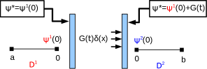
Figure 1: Cartoon of the numerical flux modification enacted at $x=0$ to solve Eq. (4). Here we show a generic time-dependent source term $G(t)\delta(x)$ “located between” subdomain red$\mathsf{D}^{1}$ and blue$\mathsf{D}^{2}$ . Interfaces are represented schematically as light blue rectangles. The advection equation (2) moves information from left-to-right, and accordingly the upwinded numerical flux is modified to the right of the delta distribution. Sec. 1 provides further discussion of the setup.

Remark When the coefficients $a_{n}(t,x)$ appearing in Eq. (1) are functions of both independent variables, they can be put into the form assumed by Theorem (2.1) by the selection property of delta distributions. For example, $a_{0}(t,x)\delta(x)=a_{0}(t,0)\delta(x)$ or $a_{1}(t,x)\delta{}^{(1)}(x)=a_{1}(t,0)\delta{}^{(1)}(x)-\partial_{x}a_{1}(t,x)\rvert_{x=0}\delta{}(x)$. Consequently, to streamline the discussion, we will exclusively focus on source terms of the form $\sum_{n=0}^{N}a_{n}(t)\delta^{(n)}(x)$ for the remainder of this paper.

2 Reduction to a first-order system

Throughout, we use both an over–dot and superscript to denote $\partial/\partial t$ differentiation, for example $\partial a/\partial t=\dot{a}(t)=a^{(1)}(t)$, and both a prime and superscript to denote $\partial/\partial x$, for example $\partial\delta/\partial x=\delta{}^{\prime}(x)=\delta^{(1)}(x)$.

2.1 Removing singular behavior

The simple advection example introduced in Sec. 1 demonstrates how to remove a certain amount of singular behavior in the source term such that the new dependent variable, $\bar{\psi}$, contains no terms proportional to $\delta(x)$. The following theorem shows how to apply the same procedure to Eq. (1).

Theorem 2.1

Consider Eq. (1) with $V=0$. Assume $a_{n}(t)$ has at least $n$ derivatives. If $\psi$ is the exact solution to Eq. (1), then

$$\bar{\psi}=\psi-\sum_{i=0}^{\frac{N-1}{2}-1}\left[\delta^{(2i)}(x)\sum_{n=0}^{\frac{N-1}{2}-1-i}a_{2n+2i+2}^{(2n)}(t)+\delta^{(2i+1)}(x)\sum_{n=0}^{\frac{N-1}{2}-1-i}a_{2n+2i+3}^{(2n)}(t)\right]\,,$$ (7)

solves

$$-\partial_{t}^{2}\bar{\psi}+\partial_{x}^{2}\bar{\psi}=G(t)\delta(x)+F(t)\delta{}^{\prime}(x)\,,$$ (8)

where

$$G(t)=\sum_{n=0}^{(N-1)/2}a_{2n}^{(2n)}(t)\,,\qquad F(t)=\sum_{n=0}^{(N-1)/2}a_{2n+1}^{(2n)}(t)\,.$$ (9)

Proof

Assume $N$ is odd, which is always possible by taking $a_{N}(t,x)=0$ if necessary. Eq. (1) can be transformed into Eq. (8) by a sequence of $\left(N-1\right)/2$ substitutions of the form

$$\bar{\psi}_{i+1}=\bar{\psi}_{i}-\sum_{n=0}^{N-2i-2}a_{n+2i+2}^{(2i)}(t)\delta^{(n)}(x)\,,$$

where we define $\bar{\psi}_{0}=\psi$. For example, we first substitute $\bar{\psi}_{1}$ into Eq. (1), generating a new wave equation for $\bar{\psi}_{1}$ with source terms proportional to $\delta^{N(x)}$ and $\delta^{N-1}(x)$ removed. Next, we substitute $\bar{\psi}_{2}$ into the PDE for $\bar{\psi}_{1}$, generating a new wave equation for ${}^{(2)}\bar{\psi}$ with the source terms proportional to $\delta^{N-2}(x)$ and $\delta^{N-3}(x)$ removed. This process continues until we arrive at an equation for $\bar{\psi}=\bar{\psi}_{(N-1)/2}$ whose source terms are $G(t)\delta(x)$ and $F(t)\delta^{(1)}(x)$. The final result can also be checked by direct computation.

Remark When $V\neq 0$ we can still remove singular behavior from the source term, although we do not provide a general expression as in Theorem 2.1. As a direct example, and assuming $V$ is differentiable, the differential equation

$$-\partial_{t}^{2}\psi+\partial_{x}^{2}\psi+V(x)\psi=a_{0}(t)\delta(x)+a_{1}(t)\delta^{(1)}(x)+a_{2}(t)\delta^{(2)}(x)+a_{3}(t)\delta^{(3)}(x)\,,$$ (10)

can be transformed into

$$-\partial_{t}^{2}\bar{\psi}+\partial_{x}^{2}\bar{\psi}+V(x)\bar{\psi}=\left[a_{0}+a_{2}^{(2)}-a_{2}V(0)+a_{3}V^{(1)}(0)\right]\delta+\left[a_{1}+a_{3}^{(2)}-a_{3}V(0)\right]\delta{}^{(1)}\,,$$ (11)

where $\bar{\psi}=\psi-a_{2}(t)\delta(x)-a_{3}(t)\delta{}^{(1)}(x)$.

2.2 First-order reduction

Thanks to Theorem 2.1, we can develop our DG method for the modified problem (8) and numerically solve for $\bar{\psi}$. At this point, we follow the approach of Ref. field2009discontinuous and introduce the auxiliary variables,

$$\hat{\phi}=\partial_{x}{\bar{\psi}}\,,\qquad\pi=-\partial_{t}\bar{\psi}\,,$$ (12)

from which the original second-order wave equation (1) can be rewritten as the following first-order system,

$$\begin{bmatrix}\bar{\psi}\\ \pi\\ \hat{\phi}\\ \end{bmatrix}_{t}+\begin{bmatrix}0&0&0\\ 0&0&1\\ 0&1&0\\ \end{bmatrix}\begin{bmatrix}\bar{\psi}\\ \pi\\ \hat{\phi}\\ \end{bmatrix}_{x}+\begin{bmatrix}\pi\\ V\bar{\psi}\\ 0\\ \end{bmatrix}=\begin{bmatrix}0\\ G(t)\delta(x)+F(t)\delta{}^{\prime}(x)\\ 0\\ \end{bmatrix}\,.$$ (13)

We find it convenient (this will be helpful in when deriving the numerical flux in Sec. 3.3) to define a new distributional auxiliary variable

$$\phi=\hat{\phi}-F(t)\delta(x)\,,$$ (14)

which removes all terms proportional to $\delta{}^{\prime}(x)$,

$$\begin{bmatrix}\bar{\psi}\\ \pi\\ \phi\\ \end{bmatrix}_{t}+\begin{bmatrix}0&0&0\\ 0&0&1\\ 0&1&0\\ \end{bmatrix}\begin{bmatrix}\bar{\psi}\\ \pi\\ \phi\\ \end{bmatrix}_{x}+\begin{bmatrix}\pi\\ V\bar{\psi}\\ 0\\ \end{bmatrix}=\begin{bmatrix}0\\ G(t)\delta(x)\\ -\dot{F}(t)\delta{}(x)\\ \end{bmatrix}\,.$$ (15)

System (15) can be written more compactly as,

$$\partial_{t}U+\partial_{x}F+\hat{V}=S(t)\delta(x)\,,$$ (16)

for the system vector $U$, flux vector $F$, potential $\hat{V}$, and source vector $S$:

$$\begin{split}U=\left[\bar{\psi},\pi,\phi\right]^{T}\,,\quad&\quad F(U)=\left[0,\phi,\pi\right]^{T}\,,\\ \hat{V}=\left[\pi,V\bar{\psi},0\right]^{T}\,,\quad&\quad S=\left[0,G(t),-\dot{F}(t)\right]^{T}\,.\end{split}$$ (17)

2.3 Distributional constraint

A solution to the first-order system (15) is also a solution to the original PDE (1) provided the distributional constraint

$$C(t,x)=\phi-\partial_{x}{\bar{\psi}}+F(t)\delta(x)\,,$$ (18)

vanishes. One can show that $C(t,x)$ obeys (upon setting $G=V=0$ for simplicity):

$$-\partial_{t}^{2}C+\partial_{x}^{2}C=0\,.$$ (19)

Thus we conclude that if the initial data implies $C(0,x)=\dot{C}(0,x)=0$, and our physical boundary condition is compatible with Eq. (18), then $C=0$ for all future times.

For certain applications, the exact initial data is unknown. If one is interested in the late-time behavior of the problem due to the forcing term, trivial initial data ($\bar{\psi}=\phi=\pi=0$) is often supplied instead. Trivial data results in an impulsive (i. e. discontinuous in time) start-up, and a key question is if a physical solution eventually emerges from such trivial initial data. The answer is unfortunately no. Under the assumption of trivial initial data we have $C(0,x)=F(0)\delta(x)$ and $\dot{C}(0,x)=0$ , giving

$$C(t,x)=\frac{1}{2}F(0)\left[\delta(x+t)+\delta(x-t)\right]\,.$$ (20)

In numerical simulations, this manifests as a localized feature that advects off the computational grid. We also observe a constraint-violating spurious (or “junk”) solution develop in it’s wake. At arbitrarily late times, the physical and numerical solution will appear to differ by a time-independent offset. To see this, let $\bar{\psi}_{\rm exact}$ be the exact particular solution to Eq. (8) and $\bar{\psi}_{\rm impulsive}$ be the solution to the first-order system (15) subject to trivial initial data. Then $\bar{\psi}_{\rm CV}=\bar{\psi}_{\rm impulsive}-\bar{\psi}_{\rm exact}$ is the spurious solution due to constraint violation. In Sec. 5 we provide numerical evidence that

$$\bar{\psi}_{\rm CV}=\frac{1}{2}F(0)\left[H(x+t)H(-x)+H(x-t)H(x)\right]\,.$$ (21)

is the spurious solution, as well as showing two ways to remove it.

3 Discontinuous Galerkin Method

To solve the wave equation (1) we first transform it into a simpler form using Theorem (2.1) then carry out a fully first-order reduction. This section describes the nodal DG method we have implemented to numerically solve the resulting system (16) subject to the constraint (18). The method is exactly the one first proposed in Ref. field2009discontinuous , and so we only briefly summarize the key ideas. Indeed, a key contribution of our paper is to show the methods of Ref. field2009discontinuous continue to be applicable for more challenging problems such as Eq. (1).

3.1 The source-free method

We divide the spatial domain into $N$ non-overlapping subdomains $a=x_{0}<x_{1}<\dots<x_{N}=b$ and denote $\mathsf{D}^{j}=[x_{j-1},x_{j}]$ as the $j^{\rm th}$ subdomain. In this one-dimensional setup, the points $\{x_{i}\}_{i=1}^{N-1}$ locate the internal subdomain interfaces, and we require one of them to be $x=0$. In each subdomain, each component of the vectors $U$, $F$, and $V$ are expanded in a polynomial basis, which are taken to be degree-$k$ Lagrange interpolating polynomials $\{\ell_{i}(x)\}_{i=0}^{k}$ defined from Legendre-Gauss-Lobatto nodes. The time-dependent coefficients of this expansion (e.g. on subdomain $j$: $\pi_{h}^{j}=\sum_{i=0}^{k}\pi_{i}(t)\ell_{i}(x)$) are the unknowns we solve for. We directly approximate $\bar{\psi}$, $\pi$, $\phi$, and $V$ and other terms arising in Eq. (16), such as $\bar{\psi}V$, are achieved through pointwise products, for example $\bar{\psi}_{h}V_{h}$.

On each subdomain, we follow the standard DG procedure by requiring the residual to satisfy

$$\int_{\mathsf{D}^{j}}\left[\frac{\partial U_{h}^{j}}{\partial_{t}}+\frac{\partial F_{h}^{j}}{\partial_{x}}+V_{h}^{j}\right]\ell_{i}^{j}dx=\left[\left(F_{h}^{j}-F^{*}\right)\ell_{i}^{j}\right]_{x_{j-1}}^{x^{j}}\,,$$ (22)

for all basis functions. Here we use an upwind numerical flux, $F^{*}(U_{h})$, that depends on the values of the numerical solution from both sides of the interface. These integrals can be pre-computed on a reference interval, leading to a coupled system of ordinary differential equations (see Eq. 47 of Ref. field2009discontinuous ) that can be integrated in time.

3.2 Modifications to the numerical flux

Figure 2: Cartoon of the numerical flux modification enacted at $x=0$ to solve Eq. (1) after its been rewritten in terms of characteristic variables (23). Here we show a generic time-dependent source term “located between” subdomain red$\mathsf{D}^{1}$ and blue$\mathsf{D}^{2}$. Interfaces are represented schematically as light blue rectangles. The system (23) includes two characteristic variables. The term $R(t)\delta(x)$ sources the right moving wave and $L(t)\delta(x)$ sources the left moving wave. The upwinded numerical flux is modified according to this directionality. Sec. 3.3 provides further discussion of the setup.

With non-zero source terms, the numerical flux evaluated at the interface $x=0$ will be modified through additional terms. The form of these new terms were derived in Eq. 58 of Ref. field2009discontinuous . Instead of reproducing those results here, we provide an alternative viewpoint leading to the same result.

We begin by writing Eq. (16) in terms of characteristic variables,

$$\begin{split}\partial_{t}w^{+}+\partial_{x}w^{+}+\frac{1}{2}V\bar{\psi}=\frac{1}{2}G(x)\delta(x)-\frac{1}{2}\dot{F}(t)\delta(x)=R(t)\delta(x)\\ \partial_{t}w^{-}-\partial_{x}w^{-}+\frac{1}{2}V\bar{\psi}=\frac{1}{2}G(x)\delta(x)+\frac{1}{2}\dot{F}(t)\delta(x)=L(t)\delta(x)\end{split}$$ (23)

where $w^{\pm}=\left(\pi\pm\phi\right)/2$ and note that $\pi=w^{+}+w^{-}$ and $\phi=w^{+}-w^{-}$. We now have two copies of an advection equation with source terms proportional to $\delta(x)$. The equation for $w^{+}$ ($w^{-}$) describes a wave moving from left-to-right (right-to-left). This allows us to apply the DG method described in the introduction: viewing the source term “between” the two subdomains, we associate the entire contribution of $R(t)$ with the subdomain to the right and the entire contribution of $L(t)$ with the subdomain to the left. Fig. 2 provides a schematic of this procedure for a simple 2 domain setup as well as the corresponding modification to the upwind numerical flux $(w^{\pm})^{*}$. Returning to the original system, the numerical flux is modified to the left (right boundary point of $\mathsf{D}^{1}$) and right (left boundary point of $\mathsf{D}^{2}$) of $\delta(x)$ by

$$F^{*}_{\rm left}\rightarrow F^{*}_{\rm left}+\left[0,-L(t),L(t)\right]^{T}\,,\qquad F^{*}_{\rm right}\rightarrow F^{*}_{\rm right}+\left[0,R(t),R(t)\right]^{T}\,.$$ (24)

3.3 Defining the Heaviside function on the DG grid

In our multi-domain setup, $x=0$ is both one of the interface locations and the location of the solution’s discontinuity. When providing initial data, for example, we will sometimes need to evaluate the Heaviside function at $x=0$. Given the expected behavior of the solution, we will evaluate the Heaviside differently depending on the problem. Consider, for example, the advection equation, $\partial_{t}\psi+\partial_{x}\psi=\cos(t)\delta^{(1)}(x)$, describing a right-moving wave and a two-subdomain setup, $\mathsf{D}^{1}=[a,0]$ and $\mathsf{D}^{2}=[0,b]$. In this case, we would evaluate the Heaviside according to $H(x)|_{\mathsf{D}^{1}}=0$ and $H(x)|_{\mathsf{D}^{2}}=1$. Now consider an advection equation describing a left-moving wave, $-\partial_{t}\psi+\partial_{x}\psi=\cos(t)\delta^{(1)}(x)$. For this problem, we would instead use $H(-x)|_{\mathsf{D}^{1}}=1$ and $H(-x)|_{\mathsf{D}^{2}}=0$.

4 Distributional solutions to the 1+1 wave equation

This section presents exact solutions to the distributionally-forced $1+1$ wave equation. These solutions will be used in Sec. 5 for testing our numerical scheme.

Our recipe for solving

$$-\partial_{t}^{2}\Psi(t,x)+\partial_{x}^{2}\Psi(t,x)=F(t)\delta^{(s)}(x)\,,$$ (25)

amounts to first solving

$$-\partial_{t}^{2}\Psi(t,x;c,s)+\partial_{x}^{2}\Psi(t,x;c,s)=F(t)\delta^{(s)}(x+c)\,,$$ (26)

for $s=0$ followed by an application of Eq. (28). We shall view $c\in\mathbb{R}$ and $s\in\mathbb{Z}_{\geq 0}$ as parameters, and the solution $\Psi(t,x;c,s)$ as parameterized by them.

A solution to (26) can be found by the method of Green’s function. Recall the fundamental solution, $G(t,x;\widetilde{t},\widetilde{x})$, for

$$-\partial_{t}^{2}G+\partial_{x}^{2}G=\delta(t-\widetilde{t})\delta(x-\widetilde{x})\,,$$

can be written in terms of the Heaviside stakgold2011green

$$G(t,x;\widetilde{t},\widetilde{x})=-\frac{1}{2}H(t-\widetilde{t}-|x-\widetilde{x}|)\,.$$

Thus the solution to Eq. (26) with $s=0$ can be written as

$$\Psi(t,x;c,s=0) =-\frac{1}{2}\int_{0}^{t}\int_{-\infty}^{\infty}H(t-\widetilde{t}-|x-\widetilde{x}|)F(\widetilde{t})\delta(\widetilde{x}+c)d\widetilde{t}d\widetilde{x}$$

$$=-\frac{1}{2}\int_{0}^{t-|x+c|}F(t-|x+c|-y)dy\,,$$ (27)

where $y=t-\widetilde{t}-|x+c|$, and we have restricted to times $t\geq 0$ for which the Heaviside is zero whenever $t-|x+c|<0$. This $s=0$ solution generates an entire family of solutions corresponding to $s>0$. Clearly $\partial_{c}^{s}\Psi(t,x;c,s=0)$ solves Eq. (26), and so the particular solution of

$$-\partial_{t}^{2}\Psi(t,x;0,s)+\partial_{x}^{2}\Psi(t,x;0,s)=F(t)\delta^{s}(x)\,,$$

is given by

$$\Psi(t,x;0,s)=\partial_{c}^{s}\Psi(t,x;c,0)\bigg{\rvert}_{c=0}\,.$$ (28)

We now provide explicit constructions for the cases considered in the numerical experiment section.

Let $F(t)=\cos(t)$ and $s=0$, then the generating function is

$$\Psi_{c}(t,x;c,0)=-\frac{1}{2}\sin(t-|x+c|)\,,$$

and setting $c=0$ gives

$$\Psi(t,x)=-\frac{1}{2}\sin(t-|x|)\,.$$

Let $F(t)=\cos(t)$ and $s=1$, then the generating function is

$$\partial_{c}\Psi_{c}(t,x;c,0)=\frac{1}{2}\mathrm{sgn}(x+c)\cos(t-|x+c|)\,,$$

and setting $c=0$ gives

$$\Psi(t,x)=\frac{1}{2}\mathrm{sgn}(x)\cos(t-|x|)\,.$$ (29)

Let $F(t)=\cos(t)$ and $s=2$, then the generating function is

$$\partial_{c}^{2}\Psi_{c}(t,x;c,0) =\delta(x+c)\cos(t-|x+c|)+\frac{1}{2}\mathrm{sgn}(x+c)\sin(t-|x+c|)\mathrm{sgn}(x+c)$$

$$=\delta(x+c)\cos(t)+\frac{1}{2}\sin(t-|x+c|)\,,$$

and setting $c=0$ gives

$$\Psi(t,x)=\delta(x)\cos(t)+\frac{1}{2}\sin(t-|x|)\,.$$ (30)

5 Numerical results

Figure 3: Convergence of the numerical solution for a sequence of grids for the problem setup described in Sec. 5.1. We consider convergence by increasing the number of elements (left) and polynomial degree (N) of the numerical approximation (right). These error profiles, computed as $\max_{x\in[-10,10]}\left|\bar{\psi}_{\rm exact}(10,x)-\bar{\psi}_{\rm numerical}(10,x)\right|$, are typical of our DG scheme when the solution is smooth. Notably, the error is also monitored at $x=0$. Left panel: For a fixed value of polynomial degree, the approximation error decreases with a power law (dashed line) at a rate which closely matches the expected rate of $-(N+1)$ (solid line). For the cases $N=\{6,7\}$, round-off error effects become noticeable around $10^{-13}$. Right panel: The DG scheme achieves exponential convergence in the approximation error as the polynomial degree is increased.

5.1 Wave equation with a $\delta^{(2)}(x)$ source term

We consider

$$-\partial_{t}^{2}\psi+\partial_{x}^{2}\psi=\cos(t)\delta^{(2)}(x)\,,$$ (31)

whose solution is given by Eq. (30). We will check the convergence of our numerically generated solution against this exact solution. Before discretization, we remove some of the equation’s singular structure by Theorem 2.1: let $\bar{\psi}=\psi-\cos(t)\delta(x)$ and solve Eq. (11) after setting $V=a_{0}=a_{1}=a_{3}=0$. At the physical boundary points we choose fluxes that enforce simple Sommerfeld boundary conditions and take the initial data from the exact solution. We solve our problem on the domain $[a,b]=[-10,10]$, set the final time T = 10, and choose a $\Delta t$ sufficiently small such that the Runge–Kutta’s timestepping error is below the spatial discretization error. Despite the exact solution being both non-smooth and containing a term proportional to $\delta(x)$, Fig. 3 shows the spectral (exponential) convergence in the approximation. For a fixed polynomial degree $k$, the scheme’s rate of convergence is observed to be $k+1$. Please see Ref. field2009discontinuous for numerical experiments with a non-zero potential.

5.2 Persistent spurious solutions from distributional constraint violations

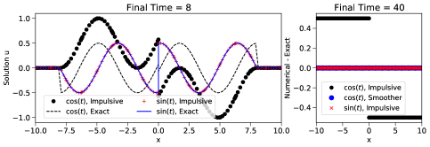
Figure 4: For certain applications, the exact initial data is unknown. Here we consider possible effects on the numerical solution when the initial data (here taken to be trivial data) leads to an impulsively started problem. The left panel shows a snapshot of the numerical solution at $T=8$ where we see that for a $\cos(t)\delta^{(1)}(x)$ source term the numerical and exact solution do not agree. In the right panel we plot the difference between the numerical and exact solution and find that the “time-independent” spurious solution that has developed is $a_{1}(0)\left[H(-x)-H(x)\right]/2$. This is not a generic feature of the problem: no spurious solution appears when the source term is smoothly turned on (right figure; blue circles) or when the when the source term is instead taken to be $\sin(t)\delta^{(1)}(x)$.

We consider

$$-\partial_{t}^{2}\psi+\partial_{x}^{2}\psi=a_{1}(t)\delta^{(1)}(x)\,,$$ (32)

for two different cases: $a_{1}(t)=\sin(t)$ and $a_{1}(t)=\cos(t)$, the latter’s exact solution is given by Eq. (29). We solve our problem on the domain $[a,b]=[-10,10]$ and we choose fluxes that enforce simple Sommerfeld boundary conditions. When the initial data is taken from the exact solution the scheme’s convergence properties are identical to those shown in Fig. 3. In light of the Sec. 2.3’s discussion on distributional constraint violations, we will check the for the appearance of persistent spurious solutions when supplying trivial initial data.

When $a_{1}(t)=\cos(t)$, the constraint violation is $C(t,x)=0.5\left[\delta(x+t)+\delta(x-t)\right]$ and the constraint-violating spurious solution

$$\bar{\psi}_{\rm CV}=\frac{1}{2}\left[H(x+t)H(-x)+H(x-t)H(x)\right]\,.$$ (33)

is the offset that develops inside the future domain influenced by $(t,x)=(0,0)$. Figure 4 (left) shows the numerical solution (black circles) offset from the exact solution (dashed black line) at $T=8$, and by $T=40$ the spurious solution has contaminated the entire computational domain (black circles). When $a_{1}(t)=\sin(t)$, the constraint violation and spurious solution vanish; this too is confirmed by Fig. 4 (red data on both left and right panels). And so we see that the problematic spurious solution can be made to vanish if it is possible to arrange the problem such that $F(0)=0$.

With neither the correct initial data nor the ability to arrange $F(0)=0$, a more general solution to this problem is to modify the source term

$$F(t)\rightarrow\left\{\begin{array}[]{rcl}f(t;\tau,\delta)F(t)&&\text{for }0\leq t\leq\tau\\ F(t)&&\text{for }t>\tau,\end{array}\right.,$$ (34)

where $f(t;\tau,\delta)={\textstyle\frac{1}{2}}[\mathrm{erf}(\sqrt{\delta}(t-\tau/2)+1]$ turns on the source term field2010persistent over the timescale $\tau$. We select $\tau=30$ and $\delta=.15$, which yields $f(0)\approx 10^{-16}$ and $f(t)=1$ for $t>30$. Both the constraint violation and spurious solution now vanish, as shown in the right panel of Fig. 4 (Blue circles).

6 Final Remarks

We have shown that the high–order accurate discontinuous Galerkin method developed in Ref. field2009discontinuous is applicable to the wave equation (1) when written in fully first-order form (16). In particular, Ref. field2009discontinuous considered a wave equation with source terms of the form $a(t,x)\delta(x)+a_{1}(t,x)\delta{}^{\prime}(x)$. In theorem 2.1 we show that one can always write Eq. (1) in this form, allowing for immediate application of their method to this generalized problem. The method maintains pointwise spectral convergence even at the source’s location where the solution may be discontinuous, singular, or both. The numerical error has been quantified by comparing against exact distributional solutions, and we have presented a procedure for finding particular solutions for any $\delta^{(n)}(x)$.

Our choice for writing the second-order scalar equation (1) in first-order form (16) relies on an auxiliary variable that must satisfy a distributional constraint (18). While this constraint vanishes for all times if it does at the initial time, for many realistic problems the initial data is not known and satisfying the distributional constraint may be challenging. For trivial initial data, we show the constraint violation advects off the computational grid, leaving behind a time-independent constraint-violating spurious (or “junk”) solution in it’s wake. We discuss two remedies that can be used to prevent the problematic spurious solution from appearing.

References

- (1) Cáceres, M.J., Carrillo, J.A., Perthame, B.: Analysis of nonlinear noisy integrate & fire neuron models: blow-up and steady states. The Journal of Mathematical Neuroscience 1(1), 1–33 (2011)
- (2) Canizares, P., Sopuerta, C.F.: Simulations of extreme-mass-ratio inspirals using pseudospectral methods. In: Journal of Physics: Conference Series, vol. 154, p. 012053. IOP Publishing (2009)
- (3) Canizares, P., Sopuerta, C.F., Jaramillo, J.L.: Pseudospectral collocation methods for the computation of the self-force on a charged particle: Generic orbits around a schwarzschild black hole. Physical Review D 82(4), 044023 (2010)
- (4) Casti, A.R.R., Omurtag, A., Sornborger, A., Kaplan, E., Knight, B., Victor, J., Sirovich, L.: A population study of integrate-and-fire-or-burst neurons. Neural computation 14(5), 957–986 (2002)
- (5) Cockburn, B.: An introduction to the Discontinuous Galerkin method for convection-dominated problems; in Advanced Numerical Approximation of Nonlinear Hyperbolic Equations: Lectures given at the 2nd Session of the Centro Internazionale Matematico Estivo (C.I.M.E.) held in Cetraro, Italy, June 23–28, 1997. Lecture Notes in Physics, pp. 150–268. Springer, Berlin, New York (1998). DOI 10.1007/BFb0096353
- (6) Cockburn, B.: Devising discontinuous Galerkin methods for non-linear hyperbolic conservation laws. J. Comput. Appl. Math. 128, 187 (2001). DOI 10.1016/S0377-0427(00)00512-4
- (7) Cockburn, B., Karniadakis, G.E., Shu, C.W.: The Development of Discontinuous Galerkin Methods; in Discontinuous Galerkin Methods: Theory, Computation and Applications. In: B. Cockburn, G.E. Karniadakis, C.W. Shu (eds.) Discontinuous Galerkin Methods: Theory, Computation and Applications, Lecture Notes in Computational Science and Engineering, pp. 3–50. Springer, Berlin, New York (2000). DOI 10.1007/978-3-642-59721-3“˙1
- (8) Cockburn, B., Shu, C.W.: The Runge-Kutta Discontinuous Galerkin Method for Conservation Laws V. Multidimensional Systems. J. Comput. Phys. 141, 199 (1998). DOI 10.1006/jcph.1998.5892
- (9) Engquist, B., Tornberg, A.K., Tsai, R.: Discretization of dirac delta functions in level set methods. Journal of Computational Physics 207(1), 28–51 (2005)
- (10) Fan, K., Cai, W., Ji, X.: A generalized discontinuous galerkin (gdg) method for schrödinger equations with nonsmooth solutions. Journal of Computational Physics 227(4), 2387–2410 (2008)
- (11) Field, S.E., Gottlieb, S., Grant, Z.J., Isherwood, L.F., Khanna, G.: A gpu-accelerated mixed-precision weno method for extremal black hole and gravitational wave physics computations. Communications on Applied Mathematics and Computation pp. 1–19 (2021)
- (12) Field, S.E., Hesthaven, J.S., Lau, S.R.: Discontinuous Galerkin method for computing gravitational waveforms from extreme mass ratio binaries. Class. Quantum Grav. 26, 165010 (2009). DOI 10.1088/0264-9381/26/16/165010
- (13) Field, S.E., Hesthaven, J.S., Lau, S.R.: Persistent junk solutions in time-domain modeling of extreme mass ratio binaries. Physical Review D 81(12), 124030 (2010)
- (14) Friedlander, F.G., Joshi, M.S., Joshi, M., Joshi, M.C.: Introduction to the Theory of Distributions. Cambridge University Press (1998)
- (15) Hesthaven, J., Warburton, T.: Nodal Discontinuous Galerkin Methods: Algorithms, Analysis, and Applications. Springer, Berlin, New York (2008). DOI 10.1007/978-0-387-72067-8
- (16) Jung, J.H., Khanna, G., Nagle, I.: A spectral collocation approximation of one-dimensional head-on collisions of black holes. Class. Quantum Gravity (2007, submitted). Also the book of abstracts of ICOSAHOM (2007)
- (17) Lousto, C.O.: A time-domain fourth-order-convergent numerical algorithm to integrate black hole perturbations in the extreme-mass-ratio limit. Classical and Quantum Gravity 22(15), S543 (2005)
- (18) Petersson, N.A., Sjogreen, B.: Stable grid refinement and singular source discretization for seismic wave simulations. Communications in Computational Physics, vol. 8, no. 5, May 31, 2010, pp. 1074-1110 8(LLNL-JRNL-419382) (2009)
- (19) Poisson, E., Pound, A., Vega, I.: The motion of point particles in curved spacetime. Living Reviews in Relativity 14(1), 1–190 (2011)
- (20) Reed, W., Hill, T.: Triangular mesh methods for the neutron transport equation. Conference: National topical meeting on mathematical models and computational techniques for analysis of nuclear systems, Ann Arbor, Michigan, USA, 8 Apr 1973 LA-UR–73-479, CONF-730414–2 (1973). URL http://www.osti.gov/scitech/servlets/purl/4491151
- (21) Shearer, P.M.: Introduction to seismology. Cambridge university press (2019)
- (22) Sopuerta, C.F., Laguna, P.: Finite element computation of the gravitational radiation emitted by a pointlike object orbiting a nonrotating black hole. Physical Review D 73(4), 044028 (2006)
- (23) Stakgold, I., Holst, M.J.: Green’s functions and boundary value problems, vol. 99. John Wiley & Sons (2011)
- (24) Sundararajan, P.A., Khanna, G., Hughes, S.A.: Towards adiabatic waveforms for inspiral into kerr black holes: A new model of the source for the time domain perturbation equation. Physical Review D 76(10), 104005 (2007)
- (25) Sundararajan, P.A., Khanna, G., Hughes, S.A., Drasco, S.: Towards adiabatic waveforms for inspiral into kerr black holes. ii. dynamical sources and generic orbits. Physical Review D 78(2), 024022 (2008)
- (26) Tornberg, A.K., Engquist, B.: Numerical approximations of singular source terms in differential equations. Journal of Computational Physics 200(2), 462–488 (2004)
- (27) Yang, Y., Shu, C.W.: Discontinuous galerkin method for hyperbolic equations involving -singularities: negative-order norm error estimates and applications. Numerische Mathematik 124(4), 753–781 (2013)