Interpreting Unfairness in Graph Neural Networks via Training Node Attribution

Abstract

Graph Neural Networks (GNNs) have emerged as the leading paradigm for solving graph analytical problems in various real-world applications. Nevertheless, GNNs could potentially render biased predictions towards certain demographic subgroups. Understanding how the bias in predictions arises is critical, as it guides the design of GNN debiasing mechanisms. However, most existing works overwhelmingly focus on GNN debiasing, but fall short on explaining how such bias is induced. In this paper, we study a novel problem of interpreting GNN unfairness through attributing it to the influence of training nodes. Specifically, we propose a novel strategy named Probabilistic Distribution Disparity (PDD) to measure the bias exhibited in GNNs, and develop an algorithm to efficiently estimate the influence of each training node on such bias. We verify the validity of PDD and the effectiveness of influence estimation through experiments on real-world datasets. Finally, we also demonstrate how the proposed framework could be used for debiasing GNNs. Open-source code can be found at https://github.com/yushundong/BIND.

Introduction

Graph data is pervasive among a plethora of realms, e.g., financial fraud detection (Wang et al. 2019; Pourhabibi et al. 2020; Cheng et al. 2020), social recommendation (Fan et al. 2019; Song et al. 2019; Guo and Wang 2020), and chemical reaction prediction (Do, Tran, and Venkatesh 2019; Shi et al. 2020; Kwon et al. 2022). As one of the state-of-the-art approaches to handle graph data, Graph Neural Networks (GNNs) have been attracting increasing attention (Kipf and Welling 2017; Hamilton, Ying, and Leskovec 2017; Veličković et al. 2017). Over the years, various graph analytical tasks have benefited from GNNs, where node classification is among the most widely studied ones (Kipf and Welling 2017; Wu et al. 2019, 2020). Nevertheless, in node classification, GNNs often yield results with discrimination towards specific demographic subgroups described by certain sensitive attributes (Dong et al. 2022a; Dai and Wang 2021a; Agarwal, Lakkaraju, and Zitnik 2021; Zhang et al. 2022b; Wang et al. 2022), such as gender, race, and religion. In many high-stake applications, critical decisions are made based on the classification results of GNNs (Shumovskaia et al. 2020), e.g., crime forecasting (Jin et al. 2020), and the exhibited bias (i.e., unfairness) is destructive for the involved individuals (Dong et al. 2022b, c; Song et al. 2022). To tackle this problem, there has been a line of works focusing on debiasing GNNs in node classification (Dong et al. 2022a; Dai and Wang 2021a; Agarwal, Lakkaraju, and Zitnik 2021; Dong et al. 2021; Loveland et al. 2022; Dai and Wang 2022). Their goal is to relieve the bias in GNN predictions on the test set and in this paper we refer to it as model bias.

In addition to debiasing GNNs, it is also critical to interpret how the model bias arises in GNNs. This is because such an understanding not only helps to determine whether a specific node should be involved in the training set, but also has much potential to guide the design of GNN debiasing methods (Dong et al. 2022a; Loveland et al. 2022; Li et al. 2021). Nevertheless, most existing GNN interpretation methods aim to understand how a prediction is made (Yuan et al. 2020b; Liu, Feng, and Hu 2022) instead of other aspects such as fairness. Consequently, although the graph data has been proved to be a significant source of model bias (Dong et al. 2022a; Li et al. 2021), existing works are unequipped to tackle this problem. In this paper, we aim to address this problem at the instance (node) level. Specifically, given a GNN trained for node classification, we aim to answer: “To what extent the GNN model bias is influenced by the existence of a specific training node in this graph?”

Nevertheless, answering the above question is technically challenging. Essentially, there are three main challenges: (1) Influence Quantification. To depict the influence of each training node on the model bias of GNNs, the first and foremost challenge is to design a principled fairness metric. A straightforward approach is to directly employ traditional fairness metrics (e.g., $\Delta_{\text{SP}}$ for Statistical Parity (Dwork et al. 2012) and $\Delta_{\text{EO}}$ for Equal Opportunity (Hardt, Price, and Srebro 2016a)). However, these metrics are not applicable in our task. The reason is that most of them are computed based on the predicted labels, while a single training node can barely twist these predicted labels on test data (Zhang et al. 2022a; Sun et al. 2020). Consequently, the influence of a single training node on the model bias would be hard to capture. (2) Computation Efficiency. To compute the influence of each training node on the model bias, a natural way is to re-train the GNN on a new graph with this specific training node being deleted and observe how the exhibited model bias changes. However, such a re-training process is prohibitively expensive. (3) Non-I.I.D. Characterization. Graph data goes against the widely adopted i.i.d. assumption, as neighboring nodes are often dependent on each other (Ma, Deng, and Mei 2021; Ying et al. 2019). Therefore, when a specific node is deleted from the graph, all its neighbors could exert different influences on the model bias of GNN during training. Such complex dependencies bring obstacles towards the analysis of node influence on the model bias.

To tackle the above challenges, in this paper, we propose a novel framework named BIND (Biased traIning Node iDentification) to quantify and estimate the influence of each training node on the model bias of GNNs. Specifically, to handle the first challenge, we propose Probabilistic Distribution Disparity (PDD) as a principled strategy to quantify the model bias. PDD directly quantifies the exhibited bias in the GNN probabilistic output instead of the predicted labels. Therefore, PDD is with finer granularity and is more suitable for capturing the influence of each specific training node compared with traditional fairness metrics. To handle the second challenge, we propose an estimation algorithm for the node influence on model bias, which avoids the re-training process and thus achieves better efficiency. To tackle the third challenge, we also characterize the dependency between nodes based on the analysis of the training loss for GNNs. Finally, experiments on real-world datasets corroborate the effectiveness of BIND. Our contributions are mainly summarized as (1) Problem Formulation. We formulate a novel problem of interpreting the bias exhibited in GNNs through attributing to the influence of training nodes; (2) Metric and Algorithm Design. We propose a novel framework BIND to quantify and efficiently estimate the influence of each training node on the model bias of GNNs; (3) Experimental Evaluation. We perform comprehensive experiments on real-world datasets to evaluate the effectiveness of the proposed framework BIND.

Preliminaries

We first present the notations used in this paper. Then, we define the problem of interpreting GNN unfairness through quantifying the influence of each specific training node.

Notations

In this paper, matrices, vectors, and scalars are represented with bold uppercase letters (e.g., $\bm{A}$), bold lowercase letters (e.g., $\bm{x}$), and normal lowercase letters (e.g., $n$), respectively.

We denote an input graph as $\mathcal{G}=\{\mathcal{V},\mathcal{E},\mathcal{X}\}$, where $\mathcal{V}=\{v_{1},...,v_{n}\}$ denotes the node set, $\mathcal{E}\subseteq\mathcal{V}\times\mathcal{V}$ represents the edge set, $\mathcal{X}=\{\bm{x}_{1},...,\bm{x}_{n}\}$ is the node attribute vectors, and $\bm{x}_{i}$ ($1\leq i\leq n$) represents the attribute vector of node $v_{i}$. We denote $\mathcal{G}_{-i}$ as the new graph with node $v_{i}$ being deleted from $\mathcal{G}$. Additionally, we employ $\mathcal{V}^{\prime}$ ($\mathcal{V}^{\prime}\subseteq\mathcal{V}$) to represent the training node set, where $|\mathcal{V}^{\prime}|=m$. The nodes in graph $\mathcal{G}$ are mapped to the output space with a trained GNN $f_{\bm{W}}$, where $\bm{W}$ represents the learnable parameters of the GNN model. We denote the optimized parameters (i.e., the parameters after training) as $\hat{\bm{W}}$. In node classification, the probabilistic classification output for the $n$ nodes is denoted as $\mathcal{\hat{Y}}=\{\hat{\bm{y}}_{1},...,\hat{\bm{y}}_{n}\}$, where $\hat{\bm{y}}_{i}\in\mathbb{R}^{c}$, and $c$ is the number of classes. We use $Y$ and $S$ to denote the ground truth label and the sensitive attribute for nodes, respectively. For an $L$-layer GNN $f_{\bm{W}}$, we define the subgraph up to $L$ hops away centered on $v_{i}$ as its computation graph (denoted as $\mathcal{G}_{i}=\{\mathcal{V}_{i},\mathcal{E}_{i},\mathcal{X}_{i}\}$). Here $\mathcal{V}_{i},\mathcal{E}_{i},$ and $\mathcal{X}_{i}$ denote the set of nodes, edges, and node attributes in $\mathcal{G}_{i}$, respectively. It is worth noting that existing works have proven that $\mathcal{G}_{i}$ fully determines the information $f_{\bm{W}}$ utilizes to make the prediction of $v_{i}$ (Ying et al. 2019). For node $v_{i}$, we use $\mathcal{V}_{i}^{\prime}$ to indicate the intersection between $\mathcal{V}_{i}$ and $\mathcal{V}^{\prime}$, i.e., $\mathcal{V}_{i}^{\prime}=\mathcal{V}_{i}\cap\mathcal{V}^{\prime}$, which is the set of training nodes in $\mathcal{G}_{i}$.

Problem Statement

The problem of interpreting GNN unfairness is formally defined as follows.

Problem 1.

GNN Unfairness Interpretation. Given the graph data $\mathcal{G}$ and a GNN model $f_{\hat{\bm{W}}}$ trained based on $\mathcal{G}$, we define the problem of interpreting GNN unfairness as to quantify the influence of each training node to the unfairness exhibited in GNN predictions on the test set.

Methodology

In this section, we first briefly introduce GNNs for the node classification task. Then, to tackle the challenge of Influence Quantification, we propose Probabilistic Distribution Disparity (PDD) to measure model bias and define node influence on the bias in a trained GNN. Furthermore, to tackle the challenge of Computation Efficiency, we design an algorithm to estimate the node influence on the model bias. Finally, we introduce how to characterize the dependency between nodes in influence estimation, which tackles the challenge of Non-I.I.D. Characterization.

GNNs in Node Classification

In the node classification task, GNNs take the input graph $\mathcal{G}$ and output a probabilistic output matrix $\hat{\bm{Y}}$, where the $i$-th row in $\hat{\bm{Y}}$ is $\hat{\bm{y}}_{i}$, i.e., the probabilistic prediction of a node’s membership over all possible classes. Usually, there are multiple layers in GNNs, where the formulation of the $l$-th layer can be summarized as:

$$\!\!\bm{z}_{i}^{(l+1)}\!=\!\sigma\left(\operatorname{AGG}\left(\bm{z}_{i}^{(l)},h\left(\left\{\bm{z}_{j}^{(l)}:v_{j}\in\mathcal{N}(v_{i})\right\}\right)\right)\right).$$ (1)

Here $\bm{z}_{i}^{(l)}$ is the embedding of node $i$ at the $l$-th layer; $\mathcal{N}(v_{i})$ is the set of one-hop neighbors around $v_{i}$; $h(\cdot)$ is a function with learnable parameters; $\operatorname{AGG}(\cdot)$ and $\sigma(\cdot)$ denote the aggregation function (e.g., mean operator) and activation function (e.g., ReLU), respectively. Later on, a loss function $L_{\mathcal{V}^{\prime}}$ (e.g., cross-entropy loss) defined on the set of training nodes $\mathcal{V}^{\prime}$ is employed for GNN training.

Probabilistic Distribution Disparity

Traditional bias metrics such as $\Delta_{\text{SP}}$ for statistical parity and $\Delta_{\text{EO}}$ for equal opportunity are computed on the predicted class labels. However, a single training node can hardly twist these predicted labels (Zhang et al. 2022a; Sun et al. 2020). Hence the node-level contribution to model bias can barely be captured by traditional bias metrics. To capture the influence of a single training node on model bias, we propose Probabilistic Distribution Disparity (PDD) as a novel bias quantification strategy. PDD can be instantiated with different fairness notions to depict the model bias from different perspectives. Specifically, we assume the population is divided into different sensitive subgroups, i.e., demographic subgroups described by the sensitive attribute. To achieve finer granularity, we define PDD as the Wasserstein-1 distance (Kantorovich 1960) between the probability distributions of a variable of interest in different sensitive subgroups. Compared with traditional fairness metrics, continuous changes brought by each specific training node are reflected in the measured distributions, and Wasserstein distance is theoretically more sensitive to the change of the measured distributions over other commonly used distribution distance metrics (Arjovsky, Chintala, and Bottou 2017). In addition, we note that the variable of interest depends on the chosen fairness notion in applications, and a larger value of PDD indicates a higher level of model bias. We introduce two instantiations of PDD based on two traditional fairness notions, including Statistical Parity (Dwork et al. 2012) and Equal Opportunity (Hardt, Price, and Srebro 2016a). Both notions are based on binary classification tasks and binary sensitive attributes (generalizations to non-binary cases can be found in Appendix A). For example, Statistical Parity requires the probability of positive predictions to be the same across two sensitive subgroups, where the variable of interest is the GNN probabilistic output $\hat{\bm{y}}$. We use $\mathcal{\hat{Y}}^{(S=j)}$ to denote the set of the probabilistic predictions for test nodes whose sensitive attribute $S$ equals to $j$ ($j\in\{0,1\}$). Let the distribution of the probabilistic predictions in $\mathcal{\hat{Y}}^{(S=0)}$ and $\mathcal{\hat{Y}}^{(S=1)}$ be $P^{(S=0)}_{\hat{\bm{y}}}$ and $P^{(S=1)}_{\hat{\bm{y}}}$, respectively. The PDD instantiated with statistical parity $\Gamma_{SP}$ is

$$\Gamma_{SP}=\text{Wasserstein}_{1}(P^{(S=0)}_{\hat{\bm{y}}},P^{(S=1)}_{\hat{\bm{y}}}),$$ (2)

where $\text{Wasserstein}_{1}(\cdot,\cdot)$ takes two distributions as input and outputs the Wasserstein-1 distance between them. Denote $Y$ as the ground truth for node classification. Similarly, we can also instantiate PDD based on Equal Opportunity $\Gamma_{EO}$ as

$$\Gamma_{EO}=\text{Wasserstein}_{1}(P^{(S=0,Y=1)}_{\hat{\bm{y}}},P^{(S=1,Y=1)}_{\hat{\bm{y}}}).$$ (3)

$P^{(S=0,Y=1)}_{\hat{\bm{y}}}$ and $P^{(S=1,Y=1)}_{\hat{\bm{y}}}$ are model prediction distributions for nodes with $(S=0,Y=1)$ and $(S=1,Y=1)$, respectively. With such a strategy, we then define node influence on model bias.

Definition 1.

Node Influence on Model Bias. Let $f_{\hat{\bm{W}}}$ and $f_{\hat{\bm{W}}^{\prime}}$ denote the GNN model trained on graph $\mathcal{G}$ and $\mathcal{G}_{-i}$ (i.e., $\mathcal{G}$ with node $v_{i}\in\mathcal{V}^{\prime}$ being deleted), respectively. Let $\Gamma_{1}$ and $\Gamma_{2}$ be the Probabilistic Distribution Disparity value based on the output of $f_{\hat{\bm{W}}}$ and $f_{\hat{\bm{W}}^{\prime}}$ for nodes in test set. We define $\Delta\Gamma=\Gamma_{2}-\Gamma_{1}$ as the influence of node $v_{i}$ on the model bias.

The rationale behind this definition is to measure to what extent $\Gamma$ changes if the GNN model is trained on a graph without $v_{i}$. Thus, $\Delta\Gamma$ depicts the influence of node $v_{i}$ on the model bias. For both instantiations of $\Gamma$ (i.e., $\Gamma_{SP}$ and $\Gamma_{EO}$), if $\Delta\Gamma>0$, deleting the training node $v_{i}$ from $\mathcal{G}$ leads to a more unfair (or biased) GNN model. This indicates that node $v_{i}$ contributes to improving the fairness level, i.e., $v_{i}$ is helpful for fairness. Nevertheless, the above computation requires re-training the GNN to obtain the influence of each training node, which is too expensive if we want to compute the influence of all nodes in the training set. In Section Node Influence on Model Bias Estimation, we introduce how to efficiently estimate $\Delta\Gamma$.

Node Influence on Model Bias Estimation

Figure 1: An illustration of how down-weighting node $v_{i}$ influences the loss values of the training nodes in $\mathcal{G}_{i}$ (including $v_{i}$, $v_{j_{1}}$, $v_{j_{2}}$, and $v_{j_{3}}$). Scenarios from $\epsilon=0$ to $\epsilon=1/m$ are presented.

It is noteworthy that PDD is a function of $\hat{\bm{W}}$ for a trained GNN, as $\hat{\bm{W}}$ directly determines the probabilistic predictions for test nodes. Hence we first characterize how a training node in $\mathcal{G}$ influences $\hat{\bm{W}}$, followed by how this node influences PDD via applying the chain rule. Formally, the optimal parameters $\hat{\bm{W}}$ minimize the objective function $L_{\mathcal{V}^{\prime}}(\mathcal{G},\bm{W})$ of the node classification task, so that:

$$\hat{\bm{W}}\stackrel{{\scriptstyle\text{ def }}}{{=}}\arg\min_{\bm{W}}L_{\mathcal{V}^{\prime}}(\mathcal{G},\bm{W})=\arg\min_{\bm{W}}\frac{1}{m}\sum_{i=1}^{m}L_{v_{i}}\left(\mathcal{G}_{i},\bm{W}\right).$$

Here $L_{v_{i}}\left(\mathcal{G}_{i},\bm{W}\right)$ denotes the loss term associated with node $v_{i}$; $\mathcal{G}_{i}$ is the computation graph of $v_{i}$; $m$ is the total number of training nodes. If a training node $v_{i}$ is deleted from $\mathcal{G}$, the loss function will change and thus leads to a different $\hat{\bm{W}}$. We take $v_{i}$ as an example to analyze the influence on $\hat{\bm{W}}$ after deleting a training node from $\mathcal{G}$. Traditionally, the existence of node $v_{i}$ is considered as a binary state, which is either one (if $v_{i}$ exists in $\mathcal{G}$) or zero (otherwise). But in our analysis, we treat it as a continuous variable to depict the intermediate states of the existence of $v_{i}$. Suppose that the existence of $v_{i}$ is down-weighted in the training of a GNN on $\mathcal{G}$. This operation leads to two changes in the loss function: (1) the loss term associated with node $v_{i}$, i.e., $L_{v_{i}}\left(\mathcal{G}_{i},\bm{W}\right)$, is down-weighted; (2) the loss terms associated with other training nodes in the computation graph of $v_{i}$ would also be influenced. The reason is that these nodes could be affected by the information from node $v_{i}$ during the message passing in GNNs (Kipf and Welling 2017; Ying et al. 2019). Based on the above analysis, we define $\hat{\bm{W}}_{\epsilon,v_{i}}$ as the optimal parameter that minimizes the loss function when node $v_{i}$ is down-weighted as follows:

$$\hat{\bm{W}}_{\epsilon,v_{i}}\stackrel{{\scriptstyle\text{ def }}}{{=}} \arg\min_{\bm{W}}L_{\mathcal{V}^{\prime}}(\mathcal{G},\bm{W})$$

$$-\epsilon\left(L_{v_{i}}\left(\mathcal{G}_{i},\bm{W}\right)+\tilde{L}_{\mathcal{V}_{i}^{\prime}}(\mathcal{G}_{i},\bm{W})\right),$$ (4)

where $\epsilon\in[0,1/m]$ controls the scale of down-weighting $v_{i}$. An illustration in Fig. 1 shows how down-weighting $v_{i}$ affects the loss values of training nodes in its computation graph. To formally characterize how node $v_{i}$ influences $\bm{\hat{W}}$, we have Theorem 1 as follows (see proofs in Appendix C).

Theorem 1.

According to the optimization objective of $\bm{\hat{W}}_{\epsilon,v_{i}}$ in Eq. (Node Influence on Model Bias Estimation), we have

$$\left.\frac{d\bm{\hat{W}}_{\epsilon,v_{i}}}{d\epsilon}\right|_{\epsilon=0}= \left(\frac{\partial^{2}L_{\mathcal{V}^{\prime}}(\mathcal{G},\hat{\bm{W}})}{\partial\bm{W}^{2}}\right)^{-1}$$

$$\cdot\left(\frac{\partial L_{v_{i}}\left(\mathcal{G}_{i},\hat{\bm{W}}\right)}{\partial\bm{W}}+\frac{\partial\tilde{L}_{\mathcal{V}_{i}^{\prime}}(\mathcal{G}_{i},\hat{\bm{W}})}{\partial\bm{W}}\right).$$ (5)

Then, we characterize the influence of down-weighting node $v_{i}$ on the value of PDD. We present Corollary 1 based on the chain rule as follows (see the proofs in Appendix C).

Corollary 1.

Define the derivative of $\Gamma$ w.r.t. $\epsilon$ at $\epsilon=0$ as $I_{\Gamma}(v_{i})$. According to Theorem 1, we have

$$\left.I_{\Gamma}(v_{i})\stackrel{{\scriptstyle\text{ def }}}{{=}}\frac{\partial\Gamma}{\partial\epsilon}\right|_{\epsilon=0}=\left(\frac{\partial\Gamma}{\partial\bm{W}}\right)^{\top}\left.\frac{d\bm{\hat{W}}_{\epsilon,v_{i}}}{d\epsilon}\right|_{\epsilon=0}.$$ (6)

With Corollary 1, we can now estimate the value change of $\Gamma$ when node $v_{i}$ is down-weighted via

$$\Gamma_{\epsilon,v_{i}}-\Gamma_{0,v_{i}}=-\epsilon\cdot I_{\Gamma}(v_{i})+o(\epsilon)\approx-\epsilon\cdot I_{\Gamma}(v_{i})$$ (7)

according to the first-order Taylor expansion. Here $\Gamma_{\epsilon,v_{i}}$ and $\Gamma_{0,v_{i}}$ are the PDD values after and before node $v_{i}$ is down-weighted, respectively. To estimate the value change in $\Gamma$ for a GNN trained on $\mathcal{G}_{-i}$, we introduce Theorem 2 as follows (see the proofs in Appendix C).

Theorem 2.

Compared with the GNN trained on $\mathcal{G}$, $\Delta\Gamma=\Gamma_{\frac{1}{m},v_{i}}-\Gamma_{0,v_{i}}$ is equivalent to the value change in $\Gamma$ when the GNN mode is trained on graph $\mathcal{G}_{-i}$.

Theorem 2 enables us to directly compute the $\Delta\Gamma$ for an arbitrary training node $v_{i}$, which helps avoid the expensive re-training process. In the next section, we further define $\tilde{L}_{\mathcal{V}_{i}^{\prime}}(\mathcal{G}_{i},\hat{\bm{W}})$ and present an algorithm to efficiently estimate the node influence on model bias.

Non-I.I.D. Characterization

Generally, there are two types of dependencies between a training node $v_{i}$ and other nodes in its computation graph $\mathcal{G}_{i}$, namely its dependency on other training nodes and its dependency on test nodes. The dependency between training nodes directly influences $\bm{W}$ during GNN training, and thus influences the probabilistic outcome of all test nodes. Hence it is critical to properly characterize the dependency between $v_{i}$ and other training nodes. Specifically, we aim to characterize how the loss summation of all training nodes in $\mathcal{G}_{i}$ changes due to the existence of $v_{i}$. We denote the training nodes other than node $v_{i}$ in $\mathcal{G}_{i}$ as $\mathcal{V}_{i}^{\prime}\backslash\{v_{i}\}$. For any node $v_{j}\in\mathcal{V}_{i}^{\prime}\backslash\{v_{i}\}$, we denote $\mathcal{G}_{j,-i}$ as the computation graph of node $v_{j}$ with node $v_{i}$ being deleted. $\tilde{L}_{\mathcal{V}_{i}}(\mathcal{G}_{i},\hat{\bm{W}})$ is then formally given as

$$\tilde{L}_{\mathcal{V}_{i}}(\mathcal{G}_{i},\hat{\bm{W}})=\sum_{v_{j}\in\mathcal{V}_{i}^{\prime}\backslash\{v_{i}\}}\left(L_{v_{j}}\left(\mathcal{G}_{j},\hat{\bm{W}}\right)-L_{v_{j}}\left(\mathcal{G}_{j,-i},\hat{\bm{W}}\right)\right).$$ (8)

The first term represents the summation of loss for nodes in $\mathcal{V}_{i}^{\prime}\backslash\{v_{i}\}$ on $\mathcal{G}$, and the second term denotes the summation of loss for these nodes on $\mathcal{G}_{-i}$. In this regard, $\tilde{L}_{\mathcal{V}_{i}}(\mathcal{G}_{i},\hat{\bm{W}})$ generally depicts to what extent the loss summation changes for nodes in $\mathcal{V}_{i}^{\prime}\backslash\{v_{i}\}$ on graph $\mathcal{G}$ compared with $\mathcal{G}_{-i}$. If $v_{i}$ is down-weighted by a certain degree, the change of the loss summation for nodes in $\mathcal{V}_{i}^{\prime}\backslash\{v_{i}\}$ can be depicted by a linearly re-scaled $\tilde{L}_{\mathcal{V}_{i}}(\mathcal{G}_{i},\hat{\bm{W}})$, as described in Eq. (Node Influence on Model Bias Estimation).

Additionally, there could also be dependencies between $v_{i}$ and test nodes in $\mathcal{G}_{i}$, as $v_{i}$ can influence the representations of its neighboring test nodes due to the information propagation mechanism in GNNs during inference. Such a dependency could also influence the value of PDD when $v_{i}$ is deleted from $\mathcal{G}$. Correspondingly, we introduce the characterization of the dependency between $v_{i}$ and test nodes. Specifically, we present an upper bound to depict the normalized change magnitude of the neighboring test nodes’ representations when a training node $v_{i}$ is deleted. Here the analysis is based on the prevalent GCN model (Kipf and Welling 2017), and can be easily generalized to other GNNs. Following widely adopted assumptions in (Huang and Zitnik 2020; Xu et al. 2018), we have Proposition 1 (see the proofs in Appendix C).

Algorithm 1 Node Influence on Model Bias Estimation

0:  $\mathcal{G}$: the graph data; $f_{\hat{\bm{W}}}$: the trained GNN model; $\mathcal{V}^{\prime}$: the set of training nodes;

0:  $\mathcal{I}_{\Gamma}=\{\Gamma_{\frac{1}{m},v_{i}}-\Gamma_{0,v_{i}}:v_{i}\in\mathcal{V}^{\prime}\}$;

1:  Initialize $\mathcal{I}_{\Gamma}=\varnothing$;

2:  Compute $\{\frac{\partial\Gamma}{\partial\bm{W}}:v_{i}\in\mathcal{V}^{\prime}\}$ based on $f_{\hat{\bm{W}}}$;

3:  while $v_{i}\in\mathcal{V}^{\prime}$ do

4:     Compute $\left.\frac{d\bm{\hat{W}}_{\epsilon,v_{i}}}{d\epsilon}\right|_{\epsilon=0}$ according to Eq. (1) and (8);

5:     Compute $I_{\Gamma}(v_{i})$ according to Eq. (6);

6:     Compute $\Gamma_{\frac{1}{m},v_{i}}-\Gamma_{0,v_{i}}$ according to Eq. (7);

7:     Append element $\Gamma_{\frac{1}{m},v_{i}}-\Gamma_{0,v_{i}}$ onto $\mathcal{I}_{\Gamma}$;

8:  end while

9:  return  $\mathcal{I}_{\Gamma}$;

Proposition 1.

Denote the representations of node $v_{j}(v_{j}\in\mathcal{V}\backslash\mathcal{V}^{\prime})$ based on $\mathcal{G}$ and $\mathcal{G}_{-i}$ as $\bm{z}_{j}$ and $\bm{z}_{j}^{\star}$, respectively. Define $h^{(j,i)}$ and $q^{(j,i)}$ as the distance from $v_{j}$ to $v_{i}$ and the number of all possible paths from $v_{j}$ to $v_{i}$, respectively. Define the set of geometric mean node degrees of $q^{(j,i)}$ paths as $\mathcal{D}=\{d_{1}^{(j,i)},...,d_{q^{(j,i)}}^{(j,i)}\}$. Define $d_{min}^{(j,i)}$ as the minimum value of $\mathcal{D}$. Assume the norms of all node representations are the same. We then have $\|\bm{z}_{j}^{\star}-\bm{z}_{j}\|_{2}/\|\bm{z}_{j}\|_{2}\leq q^{(j,i)}/(d_{min}^{(j,i)})^{h^{(j,i)}}$.

From Proposition 1, we observe that (1) deleting $v_{i}$ exerts an upper-bounded impact on the representations of other test nodes in its computation graph; and (2) this upper-bound exponentially decays w.r.t. the distance between $v_{i}$ and test nodes. Hence the dependency between $v_{i}$ and test nodes has limited influence on $\Gamma$ during inference when $v_{i}$ is deleted from the graph. On the contrary, considering that the dependency between $v_{i}$ and other training nodes directly influences $\hat{\bm{W}}$ and thus influences the inference results of all nodes, such a dependency should not be neglected. Consequently, we argue that it is reasonable to estimate the influence of each training node on $\Gamma$ by only considering the dependency between training nodes. We present the algorithmic routine of $\Delta\Gamma$ estimation in Algorithm 1.

Complexity Analysis

To better understand the computational cost, here we analyze the time complexity of estimating $\Delta\Gamma$ according to Algorithm 1. We denote the number of parameters in $\bm{W}$ and the average number of training nodes in the computation graph of an arbitrary training node as $t$ and $\bar{r}$, respectively. For each node $v_{i}$, the time complexity to compute $\partial L_{v_{i}}\left(\mathcal{G}_{i},\hat{\bm{W}}\right)/\partial\bm{W}$ and $\partial\tilde{L}_{\mathcal{V}_{i}^{\prime}}(\mathcal{G}_{i},\hat{\bm{W}})/\partial\bm{W}$ is $O$($t$) and $O$($\bar{r}t$), respectively. Hence the time complexity is $O$($m\bar{r}t$) to traverse all training nodes. For the Hessian matrix inverse, we employ a widely-used estimation approach (see Appendix A) with linear time complexity w.r.t $t$. Thus the time complexity of Eq. (1) and (8) is $O$($m\bar{r}t$). Additionally, the time complexity of Eq. (6) and (7) is $O$($mt$) and $O$($m$), respectively. To summarize, the time complexity of Algorithm 1 is $O$($m\bar{r}t$). Considering that $\bar{r}\leq m$, the algorithm has a quadratic time complexity w.r.t. training node number. This verifies the impressive time efficiency of our algorithm.

Experiments

We aim to answer the following research questions in experiments. RQ1: How efficient is BIND in estimating the influence of training nodes on the mode bias? RQ2: How well can BIND estimate the influence of training nodes on the model bias? RQ3: How well can we debias GNNs via deleting harmful training nodes based on our estimation? More details of experimental settings, supplementary experiments, and further analysis are in Appendix B.

Experimental Setup

Downstream Task & Datasets. Here the downstream task is node classification. Four real-world datasets are adopted in our experiments, including Income, Recidivism, Pokec-z, and Pokec-n. Specifically, Income is collected from Adult Data Set (Dua and Graff 2017). Each individual is represented by a node, and we establish connections (i.e., edges) between individuals following a similar criterion adopted in (Agarwal, Lakkaraju, and Zitnik 2021). The sensitive attribute is race, and the task is to classify whether the salary of a person is over $50K per year or not. Recidivism is collected from (Jordan and Freiburger 2015). A node represents a defendant released on bail, and defendants are connected based on their similarity. The sensitive attribute is race, and the task is to classify whether a defendant is on bail or not. Pokec-z and Pokec-n are collected from Pokec, which is a popular social network in Slovakia (Takac and Zabovsky 2012). In both datasets, each user is a node, and each edge stands for the friendship relation between two users. Here the locating region of users is the sensitive attribute. The task is to classify the working field of users. More details are in Appendix B.

Baselines & GNN Backbones. We compare our method with three state-of-the-art GNN debiasing baselines, namely FairGNN (Dai and Wang 2021a), NIFTY (Agarwal, Lakkaraju, and Zitnik 2021), and EDITS (Dong et al. 2022a). To perform GNN debiasing, FairGNN employs adversarial training to filter out the information of sensitive attributes from node embeddings; NIFTY maximizes the agreement between the predictions based on perturbed sensitive attributes and unperturbed ones; EDITS pre-processes the input graph data to be less biased via attribute and structural debiasing. We mainly present the results of using GCN (Kipf and Welling 2017) as the backbone GNN model, while experiments with other GNNs are discussed in Appendix B.

Evaluation Metrics. First, we employ running speedup factors to evaluate efficiency. Second, we use the widely adopted Pearson Correlation (Koh and Liang 2017; Chen et al. 2020) between the estimated and actual $\Delta\Gamma$ to evaluate the effectiveness of node influence estimation. Third, we adopt two traditional fairness metrics, namely $\Delta_{\text{SP}}$ (the metric for Statistical Parity) (Dwork et al. 2012) and $\Delta_{\text{EO}}$ (the metric for Equal Opportunity) (Hardt, Price, and Srebro 2016b), to evaluate the effectiveness of debiasing GNNs via harmful nodes deletion. Additionally, the classification accuracy is also employed to evaluate the utility-fairness trade-off.

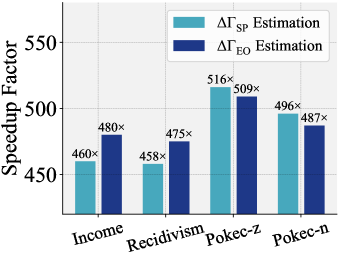
Figure 2: Evaluation of efficiency: speedup factors of $\Delta\Gamma_{\text{SP}}$ and $\Delta\Gamma_{\text{EO}}$ estimation over GNN re-training.

Efficiency of Node Influence Estimation

To answer RQ1, we evaluate the efficiency of $\Delta\Gamma$ estimation by comparing its running time with that of GNN re-training. The running time of GNN re-training is computed as follows. We first delete the target node from the original input graph $\mathcal{G}$ and re-train the GCN to obtain $f_{\hat{\bm{W}}^{\prime}}$. We then obtain $\Delta\Gamma$ based on the values of $\Gamma$ given by $f_{\hat{\bm{W}}}$ and $f_{\hat{\bm{W}}^{\prime}}$. The above running time is defined as the time cost of GNN re-training. The running time averaged across all training nodes is compared between GNN re-training and BIND, and we present the running speedup factors of BIND on the four real-world datasets in Fig. 2. We observe that the running speedup factors are over 450$\times$ on all four real-world datasets, which corroborates the efficiency superiority of BIND in estimating the value of $\Delta\Gamma$. Additionally, we observe that the estimation on Pokec-z and Pokec-n datasets has higher speedup factors on both $\Delta\Gamma_{\text{SP}}$ and $\Delta\Gamma_{\text{EO}}$ compared with the other two datasets. A reason could be that nodes in Pokec-z and Pokec-n have lower average degrees (see Appendix B). This facilitates the computation of $\tilde{L}_{\mathcal{V}_{i}^{\prime}}(\mathcal{G}_{i},\hat{\bm{W}})$ (the term that characterizes non-i.i.d.) and corresponding derivatives.

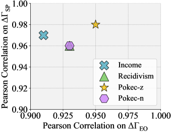
Figure 3: Evaluation of effectiveness: correlation between estimated and actual $\Delta\Gamma_{\text{SP}}$ and $\Delta\Gamma_{\text{EO}}$.

Effectiveness of Node Influence Estimation

We now evaluate the effectiveness of $\Delta\Gamma$ estimation. It is worth noting that the numerical values of the estimated influence on model bias are small for most of the nodes (see Appendix B). Here we introduce a strategy to evaluate the estimation effectiveness across a wider value range of $\Delta\Gamma$. The basic intuition here is that we select node sets and evaluate how well their estimated $\Delta\Gamma$ summation aligns with the actual one. Specifically, we first follow the widely adopted routine (Koh and Liang 2017; Chen et al. 2020) to truncate the helpful and harmful nodes with top-ranked $\Delta\Gamma$ values. We then construct a series of node sets associated with the largest positive and negative estimated $\Delta\Gamma$ summations under different set size thresholds. The range of these thresholds is between zero and a maximum possible value (determined by the training set size). It is worth noting that only nodes with non-overlapping computation graphs are selected in constructing each node set. This ensures that these nodes result in an estimated $\Delta\Gamma$ equivalent to the summation of their estimated $\Delta\Gamma$ (see Appendix C). We present the Pearson correlation of estimated $\Delta\Gamma_{\text{SP}}$ and $\Delta\Gamma_{\text{EO}}$ with the actual values on four datasets in Fig. 3. It is worth noting that achieving an exact linear correlation (i.e., Pearson correlation equals one) between the estimated and actual $\Delta\Gamma$ is almost impossible, since we only employ the first-order Taylor expansion in our estimation for $\Delta\Gamma$. From Fig. 3, we observe that the estimation achieves Pearson correlation values over 0.9 on both $\Gamma_{\text{SP}}$ and $\Gamma_{\text{EO}}$ across all datasets. Such consistencies between estimated and actual values verify the effectiveness of BIND.

Additionally, to understand how the non-i.i.d. characterization benefits the estimation, we also estimate $\Delta\Gamma$ with BIND after the non-i.i.d. characterization being disabled (i.e., setting the $\tilde{L}_{\mathcal{V}_{i}^{\prime}}(\mathcal{G}_{i},\bm{W})$ term in Eq. Node Influence on Model Bias Estimation as 0). We present the estimated $\Delta\Gamma$ v.s. actual $\Delta\Gamma$ on Income dataset with non-i.i.d. characterization being enabled and disabled in Fig. 4(a) and 4(b), respectively. We observe the correlation decreases between the estimated and actual $\Delta\Gamma$ after the non-i.i.d. characterization is disabled. Such a decrease is also observed on other datasets in terms of both statistical parity and equal opportunity. Such an observation verifies the contribution of non-i.i.d. characterization to the estimation of $\Delta\Gamma$.

Finally, we evaluate how well the values of the proposed PDD matches the values of traditional fairness metrics. We collect the value pairs of ($\Delta_{\text{SP}}$, $\Gamma_{\text{SP}}$) and ($\Delta_{\text{EO}}$, $\Gamma_{\text{EO}}$) during the GNN re-training process. The values of $\Delta_{\text{SP}}$ v.s. actual $\Gamma_{\text{SP}}$ are presented in Fig. 4(c), and the values of $\Delta_{\text{EO}}$ v.s. actual $\Gamma_{\text{EO}}$ are shown in Fig. 4(d). We observe a satisfying match between $\Gamma$ and traditional metrics, which corroborates that PDD is a valid indicator of the fairness level depicted by traditional fairness metrics.

Table 1: Comparison on GNN utility and bias mitigation between BIND and baselines. BIND 1% and BIND 10% denote the node deletion budget $k$ being $1\%$ and $10\%$ of the training node set size, respectively. ($\uparrow$) denotes the larger, the better; ($\downarrow$) denotes the opposite. Numerical results are in percentages. Best ones and runner-ups are in bold and underline, respectively.

		Van. GCN	FairGNN	NIFTY	EDITS	BIND 1%	BIND 10%
Income	($\uparrow$) Acc	74.7 $\pm$ 1.4	69.1 $\pm$ 0.6	70.8 $\pm$ 0.9	68.3 $\pm$ 0.8	75.2 $\pm$ 0.0	71.7 $\pm$ 0.7
	($\downarrow$) $\Delta_{\text{SP}}$	25.9 $\pm$ 1.9	12.4 $\pm$ 4.7	24.4 $\pm$ 1.6	24.0 $\pm$ 1.9	19.2 $\pm$ 0.6	14.7 $\pm$ 1.4
	($\downarrow$) $\Delta_{\text{EO}}$	32.3 $\pm$ 0.8	15.6 $\pm$ 6.8	26.9 $\pm$ 3.7	24.9 $\pm$ 1.0	26.4 $\pm$ 0.4	16.2 $\pm$ 2.0
Recidivism	($\uparrow$) Acc	89.8 $\pm$ 0.0	89.7 $\pm$ 0.2	79.1 $\pm$ 0.9	89.6 $\pm$ 0.1	88.7 $\pm$ 0.0	88.5 $\pm$ 0.2
	($\downarrow$) $\Delta_{\text{SP}}$	7.47 $\pm$ 0.2	7.31 $\pm$ 0.5	1.82 $\pm$ 0.8	5.02 $\pm$ 0.0	7.40 $\pm$ 0.0	6.57 $\pm$ 0.2
	($\downarrow$) $\Delta_{\text{EO}}$	5.23 $\pm$ 0.1	5.17 $\pm$ 0.0	1.28 $\pm$ 0.5	2.89 $\pm$ 0.1	5.09 $\pm$ 0.1	4.23 $\pm$ 0.2
Pokec-z	($\uparrow$) Acc	63.2 $\pm$ 0.7	64.0 $\pm$ 0.7	65.3 $\pm$ 0.2	61.6 $\pm$ 0.9	63.5 $\pm$ 0.4	62.9 $\pm$ 0.4
	($\downarrow$) $\Delta_{\text{SP}}$	7.32 $\pm$ 2.2	4.95 $\pm$ 0.8	2.34 $\pm$ 1.0	1.29 $\pm$ 0.8	6.75 $\pm$ 2.3	1.02 $\pm$ 0.9
	($\downarrow$) $\Delta_{\text{EO}}$	7.60 $\pm$ 2.3	4.29 $\pm$ 0.7	1.46 $\pm$ 1.3	1.62 $\pm$ 1.6	5.41 $\pm$ 3.4	2.28 $\pm$ 1.5
Pokec-n	($\uparrow$) Acc	58.5 $\pm$ 0.8	60.3 $\pm$ 0.5	61.1 $\pm$ 0.3	56.8 $\pm$ 0.9	60.6 $\pm$ 0.8	58.8 $\pm$ 1.8
	($\downarrow$) $\Delta_{\text{SP}}$	6.57 $\pm$ 2.6	5.30 $\pm$ 1.4	6.55 $\pm$ 0.7	2.75 $\pm$ 1.8	5.85 $\pm$ 2.0	2.45 $\pm$ 0.9
	($\downarrow$) $\Delta_{\text{EO}}$	2.33 $\pm$ 0.5	1.67 $\pm$ 0.2	1.83 $\pm$ 0.6	2.24 $\pm$ 1.5	1.15 $\pm$ 0.7	2.22 $\pm$ 1.6

(a) With non-i.i.d. term

(b) Without non-i.i.d. term

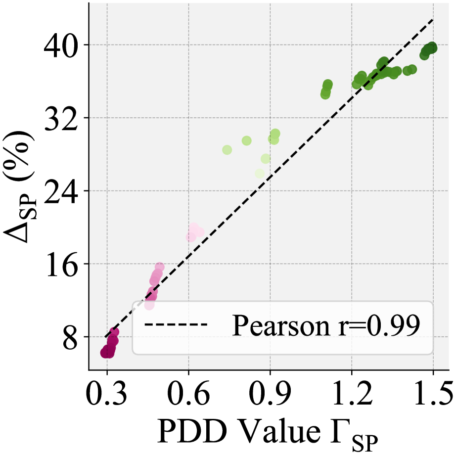
(c) $\Delta_{\text{SP}}$ v.s. $\Gamma_{\text{SP}}$ (Income)

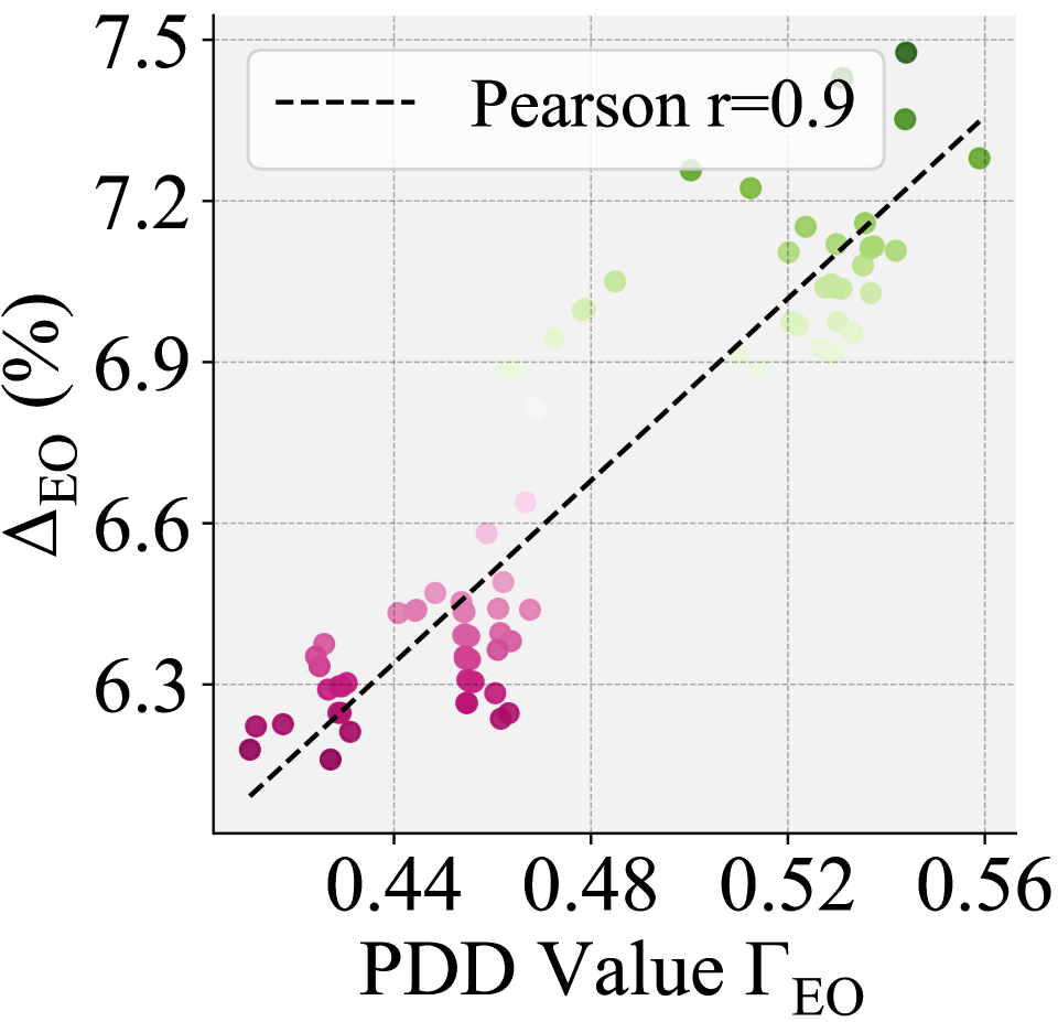
(d) $\Delta_{\text{EO}}$ v.s. $\Gamma_{\text{EO}}$ (Recid.)

Figure 4: In (a) and (b), we compare the estimation effectiveness of $\Delta\Gamma_{\text{SP}}$ with and without characterizing non-i.i.d.; in (c) and (d), we present the consistency between $\Gamma$ and traditional fairness metrics ($\Delta_{\text{SP}}$ for statistical parity and $\Delta_{\text{EO}}$ for equal opportunity) under different node deletion budgets.

Debiasing via Harmful Nodes Deletion

In this subsection, we demonstrate how BIND could be employed for GNN debiasing. The basic intuition here is to identify and delete those harmful nodes according to the estimated node influence on model bias, and evaluate whether GNNs can be debiased when they are trained on this new graph. Specifically, we set $\Gamma=\lambda\Gamma_{\text{SP}}+(1-\lambda)\Gamma_{\text{EO}}$ and estimate the node influence on $\Gamma$ to consider both statistical parity and equal opportunity. We then set a budget $k$, and follow the strategy adopted in Section Effectiveness of Node Influence Estimation to select and delete a set of training nodes with the largest positive influence summation on $\Gamma$ under this budget. We set $\lambda=0.5$ to assign statistical parity and equal opportunity the same weight, and perform experiments with $k$ being $1\%$ (denoted as BIND 1%) and $10\%$ (denoted as BIND 10%) of the total number of training nodes. We present the results on the four adopted datasets in Table 1. The following observations are made: (1) compared with other baselines, BIND achieves competitive performance (i.e., lower values) on both $\Delta_{\text{SP}}$ and $\Delta_{\text{EO}}$. Hence training GNNs on a new graph after deleting harmful nodes (to fairness) is an effective approach for GNN debiasing; (2) there is no obvious performance decrease on the model utility of BIND compared with other baselines. We thus argue that deleting harmful nodes can also lead to a satisfying fairness-utility trade-off.

Related Work

Graph Neural Networks. GNNs can be divided into spectral-based and spatial-based ones (Wu et al. 2020; Zhou et al. 2020). Spectral GNNs inherit the insights from Convolutional Neural Networks (CNNs) (Bruna et al. 2013), and it is also followed by many other works (Defferrard, Bresson, and Vandergheynst 2016; Levie et al. 2018; Kipf and Welling 2017). Their goal is to design graph filters to extract task-related information from the input graphs based on Spectral Graph Theory (Chung and Graham 1997). However, spatial GNNs design message-passing mechanisms in the spatial domain to extract information from each node’s neighbors (Wu et al. 2020; Zhou et al. 2020). Various aggregation strategies improve their performance on different tasks (Veličković et al. 2017; Xu et al. 2019b; Suresh et al. 2021; Park and Neville 2020; He et al. 2020; Schlichtkrull et al. 2018).

Algorithmic Fairness. Algorithmic fairness can be defined from different perspectives (Pessach and Shmueli 2020; M. et al. 2021; Du et al. 2020; Caton and Haas 2020; Corbett-Davies and Goel 2019; Mitchell et al. 2021), where Group Fairness and Individual Fairness are two popular notions (Dwork et al. 2012). Generally, group fairness enforces similar statistics (e.g., positive prediction rate in binary classification tasks) across different demographic subgroups (Dwork et al. 2012). Typically, these demographic subgroups are described by certain sensitive attributes, such as gender, race, and religion. On the other hand, individual fairness argues for similar outputs for similar individuals (Dwork et al. 2012). There are many works that enhance algorithmic fairness in different stages of a learning pipeline, including pre-processing (Dong et al. 2022a), in-processing (Dong et al. 2021; Lahoti, Gummadi, and Weikum 2019; Dai and Wang 2021b), and post-processing (Kang et al. 2020). Particularly, re-weighting training samples to mitigate model bias is a popular fairness-enhancing method during in-processing stage (Wang, Wu, and He 2022; Han, Baldwin, and Cohn 2021; Yan, Seto, and Apostoloff 2022; Jiang and Nachum 2020; Petrović et al. 2022). However, most of these methods only yield a set of weights for training samples to mitigate bias (Yan, Seto, and Apostoloff 2022; Wang, Wu, and He 2022), while to what extent each sample influences the exhibited bias is still unclear. Different from them, our work aims to understand the influence of each training node on model bias. To the best of our knowledge, this is a first-of-its-kind study. In addition, most of existing methods based on re-weighting training samples are developed under the IID assumption. However, in this paper, we also analyze the non-IID characteristic between nodes to better understand how each training node influences model bias.

Interpretation of Deep Learning Models. Deep learning models have huge parameter size and high complexity (Buhrmester, Münch, and Arens 2021; Samek, Wiegand, and Müller 2017; Fong and Vedaldi 2017; Xu et al. 2019a). To make these models more trustworthy and controllable, many studies have been devoted to improving their transparency (Fong and Vedaldi 2017). Generally, these works are divided into transparency design and post-hoc explanation (Xu et al. 2019a). The basic goal of transparency design is to understand the model in terms of model structure (Liu et al. 2021; Zhang et al. 2019) and training algorithms (Plumb et al. 2019), while post-hoc explanation aims to explain specific prediction results via visualization (Ding et al. 2017) and explanatory examples (Chen et al. 2018). In the realm of learning on graphs, some existing works aim to interpret GNNs (Ying et al. 2019; Luo et al. 2020; Yuan et al. 2020a), and they mainly focus on understanding the utility (e.g., node classification accuracy) of GNNs on the test set. Our work is different from them in two aspects: (1) we focus on interpreting the model bias instead of the utility for GNNs; (2) we aim to understand the model bias via attributing to the training set instead of only focusing on the test set.

Conclusion

In this paper, we study a novel problem of characterizing how each training node influences the bias exhibited in a trained GNN. We first propose a strategy named Probabilistic Distribution Disparity (PDD), which can be instantiated with different existing fairness notions, to quantify the node influence on the model bias. We then propose a novel framework named BIND to achieve an efficient influence estimation for each training node. We also develop a node deletion strategy to achieve GNN debiasing based on influence estimation. Extensive experiments verify (1) the consistency between the proposed PDD and traditional fairness metrics; (2) the efficiency and effectiveness of the influence estimation algorithm; and (3) the performance of the proposed strategy on GNN debiasing. We leave interpreting how the unfairness arises in other graph learning tasks as future works.

Supplementary Discussion

Generalized PDD Instantiations. The proposed PDD can be easily generalized to non-binary cases. Here we focus on the generalization to multi-class sensitive attributes and predicted labels. In multi-class node classification tasks with multi-class sensitive attributes, a widely adopted fairness criterion is to ensure that the ratio of predicted labels under each class is the same across all sensitive subgroups (Rahman et al. 2019; Spinelli et al. 2021) (i.e., the demographic subgroups that are described by sensitive attributes). Correspondingly, PDD can be defined as the average Wasserstein-1 distance (of the probabilistic prediction distributions) across all sensitive subgroup pairs. Here the variable of interest is $\hat{\bm{y}}$, and the generalized PDD is formally given as

$$\Gamma_{\text{generalized}}=\frac{2}{|\mathcal{S}|(|\mathcal{S}|-1)}\sum_{i\neq j\text{and}i,j\in\mathcal{S}}\text{W}_{1}(P^{(S=i)}_{\hat{\bm{y}}},P^{(S=j)}_{\hat{\bm{y}}}).$$ (9)

Here $\mathcal{S}$ is the set of all possible values for sensitive attribute $S$; W₁($\cdot,\cdot$) takes two probability distributions as input, and outputs the Wasserstein-1 distance between them; $P^{(S=i)}_{\hat{\bm{y}}}$ is the probability distribution of the GNN probabilistic predictions $\hat{\bm{y}}$ with the corresponding $S$ being $i$.

Efficient Estimation of Wasserstein Distance. Our first computation challenge lies in the notorious intractability of Wasserstein-1 distance (between two probability distributions). In additional to its intractability, the derivative of Wasserstein-1 distance between the distributions of two GNN probabilistic prediction sets w.r.t. the GNN parameters is hard to compute. To tackle both problems, we employ the efficient estimation algorithm proposed in (Cuturi and Doucet 2014), which has been widely adopted to achieve an estimation for both Wasserstein-1 distance and its derivatives w.r.t. the model parameters that are used to generate the data points from the two distributions (Ma et al. 2021; Guo, Li, and Liu 2020).

Efficient Estimation of Hessian Matrix Inverse. Our second computation challenge is the high computational cost introduced by the Hessian inverse operation in Eq. (6). To handle such a challenge, we adopt the efficient estimation approach proposed in (Martens et al. 2010), which is with linear time complexity (Koh and Liang 2017; Chen et al. 2020). Specifically, this approach estimates the product of the desired Hessian inverse and an arbitrary vector with the same dimension as the columns in the Hessian matrix, which helps to compute the multiplication between $\left(\frac{\partial^{2}L_{\mathcal{V}^{\prime}}(\mathcal{G},\hat{W})}{\partial W^{2}}\right)^{-1}$ and $\frac{\partial L_{v_{i}}\left(\mathcal{G}_{i},\hat{\bm{W}}\right)}{\partial\bm{W}}$ (or $\frac{\partial\tilde{L}_{\mathcal{V}_{i}^{\prime}}\left(\mathcal{G}_{i},\hat{W}\right)}{\partial\bm{W}}$) in Eq. (6).

Limitations & Negative Impacts. The focus of this paper is to interpret how unfairness arises in node classification tasks. However, there could also be unfairness in other graph analytical tasks. We leave this topic for future works. As for the negative impacts of this work, we do not foresee any obvious ones at this moment.

Table 2: This table presents the statistics and basic information about the four real-world datasets adopted for experimental evaluation. Sens. represents the semantic meaning of the sensitive attribute.

Dataset	Income	Recidivism	Pokec-z	Pokec-n
# Nodes	14,821	18,876	7,659	6,185
# Edges	100,483	321,308	29,476	21,844
# Attributes	14	18	59	59
Avg. degree	13.6	34.0	7.70	7.06
Sens.	Race	Race	Region	Region
Label	Income level	Bail decision	Working field	Working field

Implementation Details & Supplementary Experiments

Implementation Details

Real-world Dataset Description. There are four real-world datasets adopted in our experiments in total, namely Income, Recidivism, Pokec-z, and Pokec-n. For each dataset, there are two classes of ground truth labels (i.e., 0 and 1) for the node classification task. We randomly select 25% nodes as the validation set and 25% nodes as the test set, both of which include nodes corresponding to a balanced ratio of ground truth labels. For the training set, we randomly select either 50% nodes or 500 nodes in each class of ground truth labels, depending on which is a smaller number. Such a splitting strategy is also followed by many other works (Agarwal, Lakkaraju, and Zitnik 2021; Dong et al. 2022a). We present the statistics of the adopted datasets in Table 1. A detailed description of these datasets is as follows.

• Income. Income is collected from Adult Data Set (Dua and Graff 2017). Each individual is represented by a node. To establish edges between individuals, we first compute the Euclidean distance between every pair of individuals. For the $i$-th individual, we denote its largest Euclidean distance with other individuals as $d_{i}^{(max)}$. Then, we establish connections (i.e., edges) between the $i$-th and $j$-th individuals if their Euclidean distance in the attribute space is larger than 0.7 (edge building threshold) times min($d_{i}^{(max)}$, $d_{j}^{(max)}$). Here function min($\cdot$, $\cdot$) returns the smaller value of the two input scalars. Such a criterion of establishing connections between individuals is a widely adopted strategy in graph-based algorithmic fairness related works (Agarwal, Lakkaraju, and Zitnik 2021). The sensitive attribute is race for this dataset, and the task is to classify whether the salary of a person is over $50K per year or not.

• Recidivism. Recidivism is collected from (Jordan and Freiburger 2015). A node represents a defendant released on bail, and defendants are connected according to a similar strategy introduced in dataset Income with an edge building threshold of 0.6. The sensitive attribute is race, and the task is to classify whether a defendant is on bail or not.

• Pokec-z & Pokec-n. Pokec-z and Pokec-n are collected from Pokec, which is a popular social network in Slovakia (Takac and Zabovsky 2012). In both datasets, each user is a node, and each edge stands for the friendship relation between two users. Different from the two datasets above, the edges in these datasets are directly collected from the original data source. Here the locating region of users is the sensitive attribute, and the task is to classify the working field of users.

Figure 5: The estimated $\Delta\Gamma_{\text{SP}}$ values follow a long-tail distribution. Here, the color red and blue represent those helpful and harmful nodes, respectively.

(a) $\Delta\Gamma_{\text{SP}}$ on GIN

(b) Shuffling on GCN

Figure 6: In (a), the estimated $\Delta\Gamma_{\text{SP}}$ v.s. the actual $\Delta\Gamma_{\text{SP}}$ based on a GIN model and Income dataset is presented. In (b), we present the estimated $\Delta\Gamma_{\text{SP}}$ v.s. the actual $\Delta\Gamma_{\text{SP}}$ after randomly shuffling the order of estimated $\Delta\Gamma_{\text{SP}}$ values for the training nodes. The correlation value decrease further validates the effectiveness of estimation.

Implementation of GNNs & BIND. We present the implementation of GNNs and BIND as follows.

• GNNs. GNNs are implemented with PyTorch (Paszke et al. 2019), which is under a BSD-style license. We build all adopted GNNs with one information aggregation layer for simplicity. The information aggregation layers are implemented with PyG (PyTorch Geometric) (Fey and Lenssen 2019), which is under an MIT license license.

• BIND. BIND is implemented with PyTorch (Paszke et al. 2019), Numpy (Harris et al. 2020), and Scikit-learn (Pedregosa et al. 2011), all of which are under a BSD-style license. Code can be found in the supplementary files.

Implementation of Baselines. For all adopted GNN debiasing baselines, i.e., FairGNN, NIFTY, and EDITS, we adopt their released implementations for a fair comparison. All baselines are implemented with PyTorch (Paszke et al. 2019). FairGNN and NIFTY are optimized with Adam optimizer (Kingma and Ba 2015), while EDITS is optimized with RMSprop (Hinton, Srivastava, and Swersky 2012) as recommended.

Experimental Settings. The experiments in this paper are performed on a workstation with an Intel Exon Silver 4215 (CPU) and a Titan RTX (GPU). We set seeds as 1, 10, 100 as three runs for the replication of the experiments. For all GNNs to be interpreted, we train the GNN models for 1000 epochs with the learning rate being 1e-3. The number of the GNN hidden dimension is set as 16 for all experiments, and the dropout rate is set as 0.5. All GNNs are optimized with Adam optimizer (Kingma and Ba 2015). The iteration number for Hessian matrix inverse estimation is chosen from {10, 50, 100, 500, 1000, 5000} for the best performance.

Packages Required for Implementations. We list main packages and their corresponding versions adopted in our implementations as below.

• Python == 3.8.2

• torch == 1.7.1 + cu110

• cuda == 11.0

• torch-cluster == 1.5.9

• torch-geometric == 1.7.0

• torch-scatter == 2.0.6

• torch-sparse == 0.6.9

• tensorboard == 2.4.1

• scikit-learn == 0.23.1

• numpy == 1.19.5

• scipy==1.4.1

• networkx == 2.4

(a) $\Delta\Gamma_{\text{SP}}$ on Income

(b) $\Delta\Gamma_{\text{SP}}$ on Recidivism

(c) $\Delta\Gamma_{\text{SP}}$ on Pokec-z

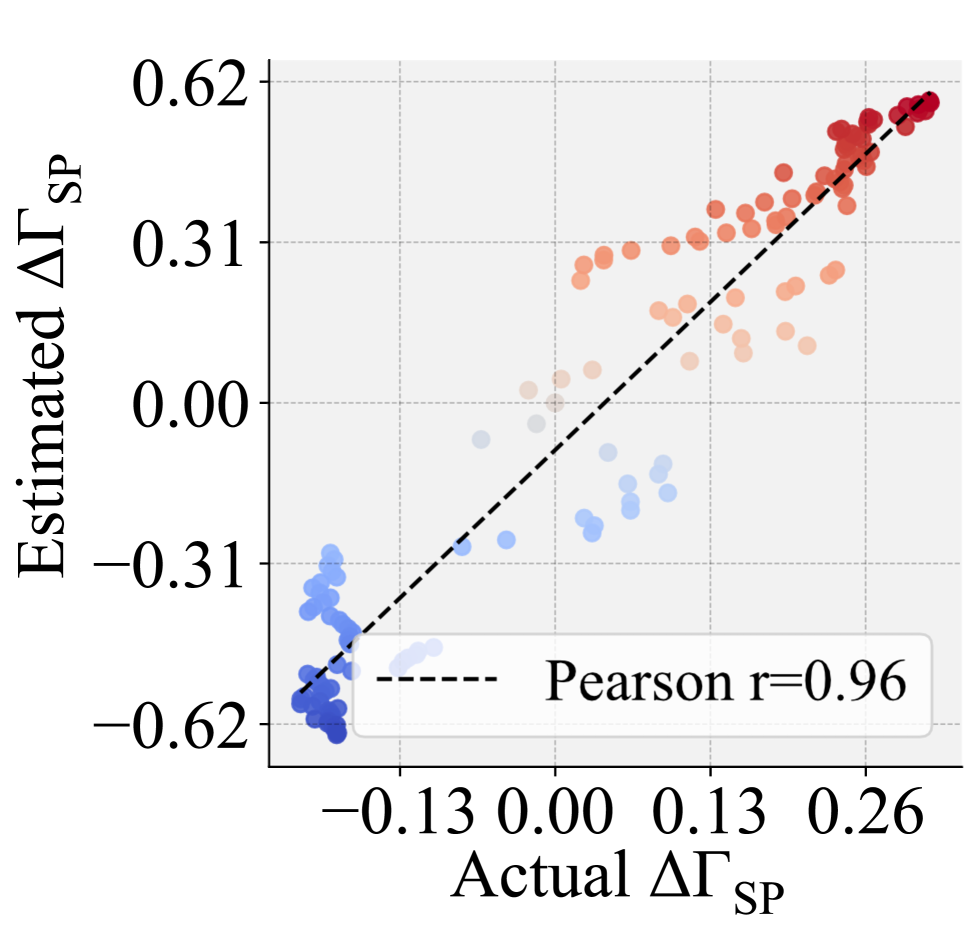
(d) $\Delta\Gamma_{\text{SP}}$ on Pokec-n

(e) $\Delta\Gamma_{\text{EO}}$ on Income

(f) $\Delta\Gamma_{\text{EO}}$ on Recidivism

(g) $\Delta\Gamma_{\text{EO}}$ on Pokec-z

(h) $\Delta\Gamma_{\text{EO}}$ on Pokec-n

Figure 7: Estimated $\Delta\Gamma$ v.s. actual $\Delta\Gamma$ on four real-world datasets are presented for effectiveness analysis of $\Delta\Gamma$ estimation based on GCN. Helpful data points (marked in red) are with positive estimated $\Delta\Gamma$ values, while harmful ones (marked in blue) are with negative estimated $\Delta\Gamma$ values.

Supplementary Experiments

Distribution of Estimated $\Delta\Gamma$. We present the estimated $\Delta\Gamma_{\text{SP}}$ on Recidivism dataset in Fig. 5. Generally, the values of the estimated node influence on bias follow a long-tail distribution, i.e., only a small amount of nodes have large positive/negative influence values on the model bias. Similar phenomena can also be observed on other datasets.

Effectiveness of $\Delta\Gamma$ Estimation. We follow the same strategy introduced in the Effectiveness of Node Influence Estimation section to obtain the estimated $\Delta\Gamma_{\text{SP}}$ values and their corresponding actual $\Delta\Gamma_{\text{SP}}$ values. We present the estimated $\Delta\Gamma_{\text{SP}}$ v.s. the actual $\Delta\Gamma_{\text{SP}}$ on the four datasets in Fig. 7(a), 7(b), 7(c), and 7(d), respectively; we also present the estimated $\Delta\Gamma_{\text{EO}}$ v.s. the actual $\Delta\Gamma_{\text{EO}}$ on the four datasets in Fig. 7(e), 7(f), 7(g), and 7(h), respectively. Experiments are carried out based on a random seed of 42. We draw the conclusion that on both $\Delta\Gamma_{\text{SP}}$ and $\Delta\Gamma_{\text{EO}}$, our estimation results show a satisfying match with the actual values across the four adopted datasets. This validates the effectiveness of $\Delta\Gamma$ estimation.

Generalization of $\Delta\Gamma$ Estimation to Different GNNs. We then test the generalization ability of our proposed estimation algorithm to different GNNs. Specifically, we present the estimated $\Delta\Gamma_{\text{SP}}$ v.s. the actual $\Delta\Gamma_{\text{SP}}$ based on a trained GIN model (Xu et al. 2019c) and Income dataset in Fig. 6(a). We have the observation that the estimated $\Delta\Gamma_{\text{SP}}$ also shows a satisfying match with the actual values based on the GIN model, which validates the generalization ability of the proposed estimation algorithm to GNNs other than GCN.

Shuffled Node Influence v.s. Actual PDD Difference. To further validate the effectiveness of the proposed estimation algorithm, we first perform node influence on bias estimation based on a trained GCN model and Income dataset. Then, we randomly shuffle the estimated influence values (i.e., estimated $\Delta\Gamma_{\text{SP}}$) for the training node set. This operation leads to a mismatch between training node indices and estimated $\Delta\Gamma_{\text{SP}}$. We follow the same strategy introduced in the Effectiveness of Node Influence Estimation section to obtain the estimated $\Delta\Gamma_{\text{SP}}$ values and their corresponding actual $\Delta\Gamma_{\text{SP}}$ values. We present the estimated $\Delta\Gamma_{\text{SP}}$ v.s. actual $\Delta\Gamma_{\text{SP}}$ in Fig. 6(b). A decrease in Pearson correlation value is observed compared with those presented in Fig. 7. This observation further corroborates the effectiveness of the proposed estimation algorithm.

Proofs

Theorem 1. According to the optimization objective of $\bm{\hat{W}}_{\epsilon,v_{i}}$ in Eq. (5), we have

$$\left.\frac{d\bm{\hat{W}}_{\epsilon,v_{i}}}{d\epsilon}\right|_{\epsilon=0}= \left(\frac{\partial^{2}L_{\mathcal{V}^{\prime}}(\mathcal{G},\hat{\bm{W}})}{\partial\bm{W}^{2}}\right)^{-1}$$

$$\cdot\left(\frac{\partial L_{v_{i}}\left(\mathcal{G}_{i},\hat{\bm{W}}\right)}{\partial\bm{W}}+\frac{\partial\tilde{L}_{\mathcal{V}_{i}^{\prime}}\left(\mathcal{G}_{i},\hat{\bm{W}}\right)}{\partial\bm{W}}\right).$$ (10)

Proof.

Here we denote $\frac{1}{m}\sum_{i=1}^{m}L_{v_{i}}\left(\mathcal{G}_{i},\bm{W}\right)$ as $L_{\mathcal{V}^{\prime}}(\mathcal{G},\bm{W})$. We also have

$$\hat{\bm{W}}_{\epsilon,v_{i}} \stackrel{{\scriptstyle\text{ def }}}{{=}}\arg\min_{\bm{W}}L_{\mathcal{V}^{\prime}}(\mathcal{G},\bm{W})$$

$$-\epsilon\left(L_{v_{i}}\left(\mathcal{G}_{i},\bm{W}\right)+\tilde{L}_{\mathcal{V}_{i}^{\prime}}\left(\mathcal{G}_{i},\bm{W}\right)\right).$$ (11)

Consequently, its first-order optimality condition holds, which is given as

$$\nabla_{\bm{W}} L_{\mathcal{V}^{\prime}}(\mathcal{G},\hat{\bm{W}}_{\epsilon,v_{i}})$$

$$-\epsilon\nabla_{\bm{W}}\left(L_{v_{i}}\left(\mathcal{G}_{i},\hat{\bm{W}}_{\epsilon,v_{i}}\right)+\tilde{L}_{\mathcal{V}_{i}^{\prime}}(\mathcal{G}_{i},\hat{\bm{W}}_{\epsilon,v_{i}})\right)=0.$$ (12)

We define

$$\Psi(\hat{\bm{W}}_{\epsilon,v_{i}}) \stackrel{{\scriptstyle\text{ def }}}{{=}}L_{\mathcal{V}^{\prime}}(\mathcal{G},\hat{\bm{W}}_{\epsilon,v_{i}})$$

$$-\epsilon\left(L_{v_{i}}\left(\mathcal{G}_{i},\hat{\bm{W}}_{\epsilon,v_{i}}\right)+\tilde{L}_{\mathcal{V}_{i}^{\prime}}(\mathcal{G}_{i},\hat{\bm{W}}_{\epsilon,v_{i}})\right)$$ (13)

for simplicity. Recall that

$$\hat{\bm{W}}\stackrel{{\scriptstyle\text{ def }}}{{=}}\arg\min_{\bm{W}}L_{\mathcal{V}^{\prime}}(\mathcal{G},\bm{W}).$$ (14)

When $\epsilon\rightarrow 0$, $\hat{\bm{W}}_{\epsilon,v_{i}}\rightarrow\hat{\bm{W}}$. According to Taylor expansion, we have

$$\nabla_{\bm{W}}\Psi(\hat{\bm{W}})+\Delta_{\epsilon,\bm{W}}\nabla_{\bm{W}}^{2}\Psi(\hat{\bm{W}})\approx 0$$ (15)

based on Eq. (Proof.), where $\Delta_{\epsilon,\bm{W}}=\hat{\bm{W}}_{\epsilon,v_{i}}-\hat{\bm{W}}$. We then can solve Eq. (15) as

$$\Delta_{\epsilon,\bm{W}}\approx-\left(\nabla_{\bm{W}}^{2}\Psi(\hat{\bm{W}})\right)^{-1}\nabla_{\bm{W}}\Psi(\hat{\bm{W}})$$ (16)

Following the simplification introduced by (Koh and Liang 2017), we drop $o$($\epsilon$) terms and let $\nabla_{\bm{W}}L_{\mathcal{V}^{\prime}}(\mathcal{G},\hat{\bm{W}})=\bm{0}$. We then have

$$\Delta_{\epsilon,\bm{W}}\approx \epsilon\left(\frac{\partial^{2}L_{\mathcal{V}^{\prime}}(\mathcal{G},\hat{W})}{\partial\bm{W}^{2}}\right)^{-1}$$

$$\cdot\left(\frac{\partial L_{v_{i}}\left(\mathcal{G}_{i},\hat{\bm{W}}\right)}{\partial\bm{W}}+\frac{\partial\tilde{L}_{\mathcal{V}_{i}^{\prime}}\left(\mathcal{G}_{i},\hat{\bm{W}}\right)}{\partial\bm{W}}\right).$$ (17)

Consequently, we have

$$\left.\frac{d\Delta_{\epsilon,\bm{W}}}{d\epsilon}\right|_{\epsilon=0}= \left(\frac{\partial^{2}L_{\mathcal{V}^{\prime}}(\mathcal{G},\hat{W})}{\partial\bm{W}^{2}}\right)^{-1}$$

$$\cdot\left(\frac{\partial L_{v_{i}}\left(\mathcal{G}_{i},\hat{\bm{W}}\right)}{\partial\bm{W}}+\frac{\partial\tilde{L}_{\mathcal{V}_{i}^{\prime}}\left(\mathcal{G}_{i},\hat{\bm{W}}\right)}{\partial\bm{W}}\right).$$ (18)

Therefore, we have

$$\left.\frac{d\Delta_{\epsilon,\bm{W}}}{d\epsilon}\right|_{\epsilon=0} =\left.\frac{d\hat{\bm{W}}_{\epsilon,v_{i}}}{d\epsilon}\right|_{\epsilon=0}-0$$

$$=\left(\frac{\partial^{2}L_{\mathcal{V}^{\prime}}(\mathcal{G},\hat{\bm{W}})}{\partial\bm{W}^{2}}\right)^{-1}$$

$$\cdot\left(\frac{\partial L_{v_{i}}\left(\mathcal{G}_{i},\hat{\bm{W}}\right)}{\partial\bm{W}}+\frac{\partial\tilde{L}_{\mathcal{V}_{i}^{\prime}}\left(\mathcal{G}_{i},\hat{\bm{W}}\right)}{\partial\bm{W}}\right).$$ (19)

∎

Corollary 1. Define the derivative of $\Gamma$ w.r.t. $\epsilon$ at $\epsilon=0$ as $I_{\Gamma}(v_{i})$. According to Theorem 1, we have

$$\left.I_{\Gamma}(v_{i})\stackrel{{\scriptstyle\text{ def }}}{{=}}\frac{\partial\Gamma}{\partial\epsilon}\right|_{\epsilon=0}=\left(\frac{\partial\Gamma}{\partial\bm{W}}\right)^{\top}\left.\frac{d\bm{\hat{W}}_{\epsilon,v_{i}}}{d\epsilon}\right|_{\epsilon=0}.$$ (20)

Proof.

$\Gamma$ is a function of $\bm{W}$, as $\Gamma$ is a function of test node representations and these representations are directly calculated based on $\bm{W}$. Assume $\Gamma$ is differentiable w.r.t. $\bm{W}$ (refer to Appendix A for the validity of this assumption). At the same time, we know $\bm{\hat{W}}_{\epsilon,v_{i}}$ is also a function of $\epsilon$, and the derivative of $\bm{\hat{W}}_{\epsilon,v_{i}}$ w.r.t. $\epsilon$ exits according to Theorem 1. As a consequence, $\Gamma$ is a function of $\epsilon$, and $\left.\frac{\partial\Gamma}{\partial\epsilon}\right|_{\epsilon=0}=\left(\frac{\partial\Gamma}{\partial\bm{W}}\right)^{\top}\left.\frac{d\bm{\hat{W}}_{\epsilon,v_{i}}}{d\epsilon}\right|_{\epsilon=0}$ according to the chain rule. ∎

Theorem 2. Compared with the GNN trained on $\mathcal{G}$, $\Delta\Gamma=\Gamma_{\frac{1}{m},v_{i}}-\Gamma_{0,v_{i}}$ is equivalent to the value change in $\Gamma$ when the GNN model is trained on graph $\mathcal{G}_{-i}$.

Proof.

Recall that

$$\hat{\bm{W}}_{\epsilon,v_{i}} \stackrel{{\scriptstyle\text{ def }}}{{=}}\arg\min_{\bm{W}}L_{\mathcal{V}^{\prime}}(\mathcal{G},\bm{W})$$

$$-\epsilon\left(L_{v_{i}}\left(\mathcal{G}_{i},\bm{W}\right)+\tilde{L}_{\mathcal{V}_{i}^{\prime}}\left(\mathcal{G}_{i},\bm{W}\right)\right).$$ (21)

When $\epsilon=\frac{1}{m}$, we define

$$\Omega(\frac{1}{m})\stackrel{{\scriptstyle\text{ def }}}{{=}}L_{\mathcal{V}^{\prime}}(\mathcal{G},\bm{W})-\frac{1}{m}L_{v_{i}}\left(\mathcal{G}_{i},\bm{W}\right)-\frac{1}{m}\tilde{L}_{\mathcal{V}_{i}^{\prime}}\left(\mathcal{G}_{i},\bm{W}\right).$$ (22)

Then, we have

$$\Omega(\frac{1}{m}) =L_{\mathcal{V}^{\prime}}(\mathcal{G},\bm{W})-\frac{1}{m}L_{v_{i}}\left(\mathcal{G}_{i},\bm{W}\right)$$

$$\;\;\;\;-\frac{1}{m}\sum_{v_{j}\in\mathcal{V}_{i}^{\prime}\backslash\left\{v_{i}\right\}}\left(L_{v_{j}}\left(\mathcal{G}_{j},\bm{W}\right)-L_{v_{j}}\left(\mathcal{G}_{j,-i},\bm{W}\right)\right)$$

$$=\frac{1}{m}\sum_{v_{j}\notin\mathcal{V}_{i}^{\prime}}L_{v_{j}}\left(\mathcal{G}_{j},\bm{W}\right)$$

$$\;\;\;\;+\frac{1}{m}\sum_{v_{j}\in\mathcal{V}_{i}^{\prime}\backslash\left\{v_{i}\right\}}L_{v_{j}}\left(\mathcal{G}_{j,-i},\bm{W}\right),$$ (23)

where $\mathcal{G}_{j,-i}$ is the computation graph of $v_{j}$ with $v_{i}$ being removed. As a consequence, $\Omega(\frac{1}{m})$ is the loss function based on $\mathcal{G}_{-i}$, i.e., $\mathcal{G}$ with node $v_{i}$ being removed. Correspondingly, $\Delta\Gamma=\Gamma_{\frac{1}{m},v_{i}}-\Gamma_{0,v_{i}}$ is equivalent to the value change in $\Gamma$ when the GNN model is trained on graph $\mathcal{G}_{-i}$. ∎

Proposition 1. Denote the learned representations of node $v_{j}(v_{j}\in\mathcal{V}\backslash\mathcal{V}^{\prime})$ based on $\mathcal{G}$ and $\mathcal{G}_{-i}$ as $\bm{z}_{j}$ and $\bm{z}_{j}^{\star}$, respectively. Define $h^{(j,i)}$ and $q^{(j,i)}$ as the distance from $v_{j}$ to $v_{i}$ and the number of all possible paths from $v_{j}$ to $v_{i}$, respectively. Define the set of geometric mean node degrees of $q^{(j,i)}$ paths as $\mathcal{D}=\{d_{1}^{(j,i)},...,d_{q^{(j,i)}}^{(j,i)}\}$. Define $d_{min}^{(j,i)}$ as the minimum value of $\mathcal{D}$. Assume the norms of all node representations are the same. We then have $\|\bm{z}_{j}^{\star}-\bm{z}_{j}\|_{2}/\|\bm{z}_{j}\|_{2}\leq q^{(j,i)}/(d_{min}^{(j,i)})^{h^{(j,i)}}$.

Proof.

In the following proof, we will follow (Huang and Zitnik 2020) and (Xu et al. 2018) to use GCNs as the exemplar GNN of this proof for simplicity. However, our proof can also be naturally generalized to other GNNs (e.g., GAT (Veličković et al. 2017) and GraphSAGE (Hamilton, Ying, and Leskovec 2017)) by choosing different values for edge weights. Specifically, the $l$-th layer propagation process can be represented as $\mathbf{H}^{(l+1)}=\sigma(\hat{\mathbf{A}}\mathbf{H}^{(l)}\mathbf{W}^{(l})$, where $\mathbf{H}^{(l)}$ and $\mathbf{W}^{(l)}$ denote the node representation and weight parameter matrices, respectively. $\hat{\mathbf{A}}=\mathbf{D}^{-1}\mathbf{A}$ is the adjacency matrix after row normalization. Following (Huang and Zitnik 2020), (Wang and Leskovec 2020), and (Xu et al. 2018), we set $\sigma$ as an identity function and $\mathbf{W}$ an identity matrix. According to the Taylor’s theorem, we have

$$\begin{aligned} \bm{z}_{j}^{\star}-\bm{z}_{j}\approx\frac{\partial\bm{z}_{j}}{\partial\bm{z}_{i}}\bm{z}_{i}\end{aligned}.$$ (24)

To calculate $\frac{\partial\bm{z}_{j}}{\partial\bm{z}_{i}}$, we can expand the $\bm{z}_{j}$ according to the propagation rule. Then we have

$$\frac{\partial\bm{z}_{j}}{\partial\bm{z}_{i}} =\frac{\partial}{\partial\bm{z}_{i}}\left(\frac{1}{D_{jj}}\sum\limits_{k\in\mathcal{N}(j)}a_{jk}\ \dotsi\ \frac{1}{D_{mm}}\sum\limits_{o\in\mathcal{N}(m)}a_{mo}\bm{z}_{o}\right)$$

$$=\frac{\partial}{\partial\bm{z}_{i}}\left(\sum\limits_{k=1}^{l}\sum\limits_{\mathcal{P}^{j\rightarrow i}_{k}}\prod_{o=k}^{1}\tilde{a}_{v_{(o-1)},v_{(o)}}\bm{z}_{i}\right)$$

$$=\frac{\partial}{\partial\bm{z}_{i}}\left(\sum\limits_{p=1}^{q}\prod_{o=k_{p}}^{1}\tilde{a}_{v^{(p)}_{(o-1)},v^{(p)}_{(o)}}\bm{z}_{i}\right).$$ (25)

Here, we substitute the term $\bm{z}_{j}$ by expansion based on the GCN propagation rule. $\mathcal{P}^{j\rightarrow i}_{k}$ is a path $[v_{(k)},v_{(k-1)},\dotsc,v_{(0)}]$ of length $k$ from node $v_{j}$ to $v_{i}$, where $v_{(k)}=v_{j}$ and $v_{(0)}=v_{i}$. Moreover, $v_{(o-1)}\in\mathcal{N}\left(v_{(o)}\right)$ for $o=k,k-1,\dotsc,1$. $\tilde{a}_{v_{(o-1)},v_{(o)}}$ denotes the normalized edge weight between $v^{(p)}_{(o-1)}$ and $v^{(p)}_{(o)}$. $k_{p}$ is the length of the $p$-th path, and we denote node $v_{(o)}$ in the $p$-th path as $v^{(p)}_{(o)}$. In this expansion, we first aggregate all paths from $v_{j}$ to $v_{i}$ of different lengths (with a maximum length of $l$) and ignore other paths that end at other nodes. This is because we only consider the gradient between $v_{j}$ and $v_{i}$. In other words, the derivative on other paths will be 0. Denoting the total number of such paths as $q^{(j,i)}$, we can further extract $\partial\bm{z}_{i}/\partial\bm{z}_{i}$ as follows:

$$\frac{\partial\bm{z}_{j}}{\partial\bm{z}_{i}} =\frac{\partial\bm{z}_{i}}{\partial\bm{z}_{i}}\cdot\left(\sum\limits_{p=1}^{q^{(j,i)}}\prod_{o=k_{p}}^{1}\tilde{a}_{v^{(p)}_{(o-1)},v^{(p)}_{(o)}}\right)$$ (26)

$$=\mathbf{I}\cdot\left(\sum\limits_{p=1}^{q^{(j,i)}}\prod_{o=k_{p}}^{1}\tilde{a}_{v^{(p)}_{(o-1)},v^{(p)}_{(o)}}\right).$$

Therefore, we have

$$\frac{\|\bm{z}_{j}^{\star}-\bm{z}_{j}\|_{2}}{\|\bm{z}_{j}\|_{2}} \approx\|\frac{\partial\bm{z}_{j}}{\partial\bm{z}_{i}}\bm{z}_{i}\|_{2}\cdot\frac{1}{\|\bm{z}_{j}\|_{2}}$$ (27)

$$=\left(\sum\limits_{p=1}^{q^{(j,i)}}\prod_{o=k_{p}}^{1}\tilde{a}_{v^{(p)}_{(o-1)},v^{(p)}_{(o)}}\right)\frac{\|\bm{z}_{i}\|_{2}}{\|\bm{z}_{j}\|_{2}}.$$

In the above equations, the value of $\|\bm{z}_{i}\|_{2}/\|\bm{z}_{j}\|_{2}$ becomes 1 since all norms are the same. Then we select the path with the largest value of $\prod_{o=k}^{1}\tilde{a}_{v_{(o-1)},v_{(o)}}$ from all $q^{(j,i)}$ possible paths starting from $v_{j}$ to $v_{i}$, denoted as path $p_{*}$:

$$\sum\limits_{p=1}^{q^{(j,i)}}\prod_{o=k_{p}}^{1}\tilde{a}_{v^{(p)}_{(o-1)},v^{(p)}_{(o)}} \leq q^{(j,i)}\cdot\max\left(\prod_{o=k_{1}}^{1}\tilde{a}_{v^{(1)}_{(o-1)},v^{(1)}_{(o)}},\ \right.$$

$$\;\;\;\;\left.\dotsi,\ \prod_{o=k_{m}}^{1}\tilde{a}_{v^{(q^{(j,i)})}_{(o-1)},v^{(q^{(j,i)})}_{(o)}}\right)$$

$$=q^{(j,i)}\cdot\left(\prod_{o=k_{p_{*}}}^{1}\tilde{a}_{v^{(p_{*})}_{(o-1)},v^{(p_{*})}_{(o)}}\right).$$ (28)

Here $k_{p_{*}}$ is the length of path $p_{*}$. Since the edge weight is 1 on the path, we can remove the expression of $a$ as follows:

$$\sum\limits_{p=1}^{q^{(j,i)}}\prod_{o=k_{p}}^{1}\tilde{a}_{v^{(p)}_{(o-1)},v^{(p)}_{(o)}} \leq q^{(j,i)}\cdot\left(\prod_{o=k_{p_{*}}}^{1}\frac{1}{D^{(p_{*})}_{(o),(o)}}\right)$$ (29)

$$=q^{(j,i)}\cdot\left(\sqrt[k_{p_{*}}]{\prod_{o=k_{p_{*}}}^{1}D^{(p_{*})}_{(o),(o)}}\right)^{-k_{p_{*}}}.$$

Combining with Eq. (27), we can obtain

$$\frac{\|\bm{z}_{j}^{\star}-\bm{z}_{j}\|_{2}}{\|\bm{z}_{j}\|_{2}} \approx\left(\sum\limits_{p=1}^{q^{(j,i)}}\prod_{o=k_{p}}^{1}\tilde{a}_{v^{(p)}_{(o-1)},v^{(p)}_{(o)}}\right)$$ (30)

$$\leq q^{(j,i)}/(d_{min}^{(j,i)})^{k_{p_{*}}}$$

$$\leq q^{(j,i)}/(d_{min}^{(j,i)})^{h^{(j,i)}},$$

where $d_{min}^{(j,i)}$ is the geometric mean of node degrees on path $p_{*}$. Then, we can further utilize $h^{(j,i)}$, which is the shortest path between $v_{j}$ and $v_{i}$, to obtain the inequality. It is worth mentioning that since we do not explicitly restrict the values of edge weights, our proof can be generalized to other GNNs by choosing appropriate values for the edge weights. ∎

Theorem 3. Denote $I_{\Gamma}(\tilde{\mathcal{V}})$ as the summation of influence scores to the PDD for node set $\tilde{\mathcal{V}}$. Given a node set $\tilde{\mathcal{V}}\subseteq\mathcal{V}^{\prime}$ ($|\tilde{\mathcal{V}}|=k$), if $\mathcal{V}_{x}^{\prime}\cap\mathcal{V}_{y}^{\prime}=\varnothing$ holds for any pair of nodes $v_{x},v_{y}\in\tilde{\mathcal{V}}$ ($x\neq y$), then $I_{\Gamma}(\tilde{\mathcal{V}})=\sum_{v_{i}\in\tilde{\mathcal{V}}}I_{\Gamma}(v_{i})$.

Proof.

Recall that

$$\hat{\bm{W}}_{\epsilon,v_{i}} \stackrel{{\scriptstyle\text{ def }}}{{=}}\arg\min_{\bm{W}}L_{\mathcal{V}^{\prime}}(\mathcal{G},\bm{W})$$

$$-\epsilon\left(L_{v_{i}}\left(\mathcal{G}_{i},\bm{W}\right)+\tilde{L}_{\mathcal{V}_{i}^{\prime}}\left(\mathcal{G}_{i},\bm{W}\right)\right).$$ (31)

Considering the computation graphs of any two nodes in $\tilde{\mathcal{V}}$ do not overlap with each other, each node $v_{i}$ in $\tilde{\mathcal{V}}$ corresponds to a term of $L_{v_{i}}\left(\mathcal{G}_{i},\bm{W}\right)+\tilde{L}_{\mathcal{V}_{i}^{\prime}}\left(\mathcal{G}_{i},\bm{W}\right)$ that is non-dependent on other training nodes (or the training nodes in their computation graphs) to be deleted. Therefore, the nodes in set $\tilde{\mathcal{V}}$ correspond to a linear sum of the $L_{v_{i}}\left(\mathcal{G}_{i},\bm{W}\right)+\tilde{L}_{\mathcal{V}_{i}^{\prime}}\left(\mathcal{G}_{i},\bm{W}\right)$ term. Consequently, we have

$$I_{G}(\tilde{\mathcal{V}}) =-\left(\frac{\partial G}{\partial\bm{\hat{W}}_{\epsilon,\tilde{\mathcal{V}}}}\right)^{\top}\cdot\left(\frac{\partial^{2}L_{\mathcal{V}^{\prime}}(\mathcal{G},\bm{W})}{\partial\bm{W}^{2}}\right)^{-1}$$

$$\;\;\;\;\cdot\left(\sum_{k=1}^{K}\frac{\partial L_{v_{i_{k}}}\left(\mathcal{G}_{i_{k}},\bm{W}\right)}{\partial\bm{W}}+\sum_{k=1}^{K}\frac{\partial\tilde{L}_{\mathcal{V}_{i_{k}}^{\prime}}(\mathcal{G}_{i_{k}},\bm{W})}{\partial\bm{W}}\right)$$

$$=-\sum_{k=1}^{K}\left(\frac{\partial G}{\partial\bm{\hat{W}}_{\epsilon,\tilde{\mathcal{V}}}}\right)^{\top}\cdot\left(\frac{\partial^{2}L_{\mathcal{V}^{\prime}}(\mathcal{G},\bm{W})}{\partial\bm{W}^{2}}\right)^{-1}$$

$$\;\;\;\;\cdot\left(\frac{\partial L_{v_{i_{k}}}\left(\mathcal{G}_{i_{k}},\bm{W}\right)}{\partial\bm{W}}+\frac{\partial\tilde{L}_{\mathcal{V}_{i_{k}}^{\prime}}(\mathcal{G}_{i_{k}},\bm{W})}{\partial\bm{W}}\right)$$

$$=\sum_{k=1}^{K}I_{G}(v_{i_{k}}).$$ (32)

∎

References

- Agarwal, Lakkaraju, and Zitnik (2021) Agarwal, C.; Lakkaraju, H.; and Zitnik, M. 2021. Towards a Unified Framework for Fair and Stable Graph Representation Learning. In UAI.
- Arjovsky, Chintala, and Bottou (2017) Arjovsky, M.; Chintala, S.; and Bottou, L. 2017. Wasserstein GAN. In ICML.
- Bruna et al. (2013) Bruna, J.; Zaremba, W.; Szlam, A.; and LeCun, Y. 2013. Spectral networks and locally connected networks on graphs. arXiv preprint arXiv:1312.6203.
- Buhrmester, Münch, and Arens (2021) Buhrmester, V.; Münch, D.; and Arens, M. 2021. Analysis of explainers of black box deep neural networks for computer vision: A survey. MLKE.
- Caton and Haas (2020) Caton, S.; and Haas, C. 2020. Fairness in machine learning: A survey. CSUR.
- Chen et al. (2020) Chen, H.; Si, S.; Li, Y.; Chelba, C.; Kumar, S.; Boning, D.; and Hsieh, C.-J. 2020. Multi-stage influence function. NeurIPS.
- Chen et al. (2018) Chen, J.; Song, L.; Wainwright, M.; and Jordan, M. 2018. Learning to explain: An information-theoretic perspective on model interpretation. In ICML.
- Cheng et al. (2020) Cheng, D.; Wang, X.; Zhang, Y.; and Zhang, L. 2020. Graph neural network for fraud detection via spatial-temporal attention. TKDE.
- Chung and Graham (1997) Chung, F. R.; and Graham, F. C. 1997. Spectral graph theory. 92. American Mathematical Soc.
- Corbett-Davies and Goel (2019) Corbett-Davies, S.; and Goel, S. 2019. The measure and mismeasure of fairness: A critical review of fair machine learning. In NeurIPS.
- Cuturi and Doucet (2014) Cuturi, M.; and Doucet, A. 2014. Fast computation of Wasserstein barycenters. In ICML.
- Dai and Wang (2021a) Dai, E.; and Wang, S. 2021a. Say no to the discrimination: Learning fair graph neural networks with limited sensitive attribute information. In WSDM.
- Dai and Wang (2021b) Dai, E.; and Wang, S. 2021b. Towards Self-Explainable Graph Neural Network. In CIKM.
- Dai and Wang (2022) Dai, E.; and Wang, S. 2022. Learning fair graph neural networks with limited and private sensitive attribute information. TKDE.
- Defferrard, Bresson, and Vandergheynst (2016) Defferrard, M.; Bresson, X.; and Vandergheynst, P. 2016. Convolutional neural networks on graphs with fast localized spectral filtering. NeurIPS.
- Ding et al. (2017) Ding, Y.; Liu, Y.; Luan, H.; and Sun, M. 2017. Visualizing and understanding neural machine translation. In ACL.
- Do, Tran, and Venkatesh (2019) Do, K.; Tran, T.; and Venkatesh, S. 2019. Graph transformation policy network for chemical reaction prediction. In SIGKDD.
- Dong et al. (2021) Dong, Y.; Kang, J.; Tong, H.; and Li, J. 2021. Individual Fairness for Graph Neural Networks: A Ranking based Approach. In SIGKDD.
- Dong et al. (2022a) Dong, Y.; Liu, N.; Jalaian, B.; and Li, J. 2022a. EDITS: Modeling and Mitigating Data Bias for Graph Neural Networks. In The Web Conf.
- Dong et al. (2022b) Dong, Y.; Ma, J.; Chen, C.; and Li, J. 2022b. Fairness in Graph Mining: A Survey. arXiv preprint arXiv:2204.09888.
- Dong et al. (2022c) Dong, Y.; Wang, S.; Wang, Y.; Derr, T.; and Li, J. 2022c. On Structural Explanation of Bias in Graph Neural Networks. In KDD.
- Du et al. (2020) Du, M.; Yang, F.; Zou, N.; and Hu, X. 2020. Fairness in deep learning: A computational perspective. IEEE Intelligent Systems.
- Dua and Graff (2017) Dua, D.; and Graff, C. 2017. UCI Machine Learning Repository.
- Dwork et al. (2012) Dwork, C.; Hardt, M.; Pitassi, T.; Reingold, O.; and Zemel, R. 2012. Fairness through awareness. In ITCS.
- Fan et al. (2019) Fan, W.; Ma, Y.; Li, Q.; He, Y.; Zhao, E.; Tang, J.; and Yin, D. 2019. Graph neural networks for social recommendation. In The Web Conf.
- Fey and Lenssen (2019) Fey, M.; and Lenssen, J. E. 2019. Fast Graph Representation Learning with PyTorch Geometric. In ICLR Workshop on Representation Learning on Graphs and Manifolds.
- Fong and Vedaldi (2017) Fong, R. C.; and Vedaldi, A. 2017. Interpretable explanations of black boxes by meaningful perturbation. In ICCV.
- Guo, Li, and Liu (2020) Guo, R.; Li, J.; and Liu, H. 2020. Learning individual causal effects from networked observational data. In WSDM.
- Guo and Wang (2020) Guo, Z.; and Wang, H. 2020. A deep graph neural network-based mechanism for social recommendations. TKDE.
- Hamilton, Ying, and Leskovec (2017) Hamilton, W.; Ying, Z.; and Leskovec, J. 2017. Inductive representation learning on large graphs. In NeurIPS.
- Han, Baldwin, and Cohn (2021) Han, X.; Baldwin, T.; and Cohn, T. 2021. Balancing out Bias: Achieving Fairness Through Balanced Training. arXiv preprint arXiv:2109.08253.
- Hardt, Price, and Srebro (2016a) Hardt, M.; Price, E.; and Srebro, N. 2016a. Equality of Opportunity in Supervised Learning. In NeurIPS.
- Hardt, Price, and Srebro (2016b) Hardt, M.; Price, E.; and Srebro, N. 2016b. Equality of opportunity in supervised learning. In NeurIPS.
- Harris et al. (2020) Harris, C. R.; Millman, K. J.; van der Walt, S. J.; Gommers, R.; Virtanen, P.; Cournapeau, D.; Wieser, E.; Taylor, J.; Berg, S.; Smith, N. J.; Kern, R.; Picus, M.; Hoyer, S.; van Kerkwijk, M. H.; Brett, M.; Haldane, A.; del Río, J. F.; Wiebe, M.; Peterson, P.; Gérard-Marchant, P.; Sheppard, K.; Reddy, T.; Weckesser, W.; Abbasi, H.; Gohlke, C.; and Oliphant, T. E. 2020. Array programming with NumPy. Nature.
- He et al. (2020) He, X.; Deng, K.; Wang, X.; Li, Y.; Zhang, Y.; and Wang, M. 2020. Lightgcn: Simplifying and powering graph convolution network for recommendation. In SIGIR.
- Hinton, Srivastava, and Swersky (2012) Hinton, G.; Srivastava, N.; and Swersky, K. 2012. Neural networks for machine learning lecture 6a overview of mini-batch gradient descent.
- Huang and Zitnik (2020) Huang, K.; and Zitnik, M. 2020. Graph meta learning via local subgraphs. In NeurIPS.
- Jiang and Nachum (2020) Jiang, H.; and Nachum, O. 2020. Identifying and correcting label bias in machine learning. In AISTATS.
- Jin et al. (2020) Jin, G.; Wang, Q.; Zhu, C.; Feng, Y.; Huang, J.; and Zhou, J. 2020. Addressing crime situation forecasting task with temporal graph convolutional neural network approach. In ICMTMA.
- Jordan and Freiburger (2015) Jordan, K. L.; and Freiburger, T. L. 2015. The effect of race/ethnicity on sentencing: Examining sentence type, jail length, and prison length. J Crim Justice.
- Kang et al. (2020) Kang, J.; He, J.; Maciejewski, R.; and Tong, H. 2020. Inform: Individual fairness on graph mining. In SIGKDD.
- Kantorovich (1960) Kantorovich, L. V. 1960. Mathematical methods of organizing and planning production. Management science.
- Kingma and Ba (2015) Kingma, D. P.; and Ba, J. 2015. Adam: A Method for Stochastic Optimization. In ICLR.
- Kipf and Welling (2017) Kipf, T. N.; and Welling, M. 2017. Semi-Supervised Classification with Graph Convolutional Networks. In ICLR.
- Koh and Liang (2017) Koh, P. W.; and Liang, P. 2017. Understanding black-box predictions via influence functions. In ICML.
- Kwon et al. (2022) Kwon, Y.; Lee, D.; Choi, Y.-S.; and Kang, S. 2022. Uncertainty-aware prediction of chemical reaction yields with graph neural networks. Journal of Cheminformatics.
- Lahoti, Gummadi, and Weikum (2019) Lahoti, P.; Gummadi, K. P.; and Weikum, G. 2019. iFair: Learning Individually Fair Data Representations for Algorithmic Decision Making. In ICDE.
- Levie et al. (2018) Levie, R.; Monti, F.; Bresson, X.; and Bronstein, M. M. 2018. Cayleynets: Graph convolutional neural networks with complex rational spectral filters. IEEE Trans. Signal Process.
- Li et al. (2021) Li, P.; Wang, Y.; Zhao, H.; Hong, P.; and Liu, H. 2021. On dyadic fairness: Exploring and mitigating bias in graph connections. In ICLR.
- Liu et al. (2021) Liu, G.; Sun, X.; Schulte, O.; and Poupart, P. 2021. Learning Tree Interpretation from Object Representation for Deep Reinforcement Learning. NeurIPS.
- Liu, Feng, and Hu (2022) Liu, N.; Feng, Q.; and Hu, X. 2022. Interpretability in Graph Neural Networks.
- Loveland et al. (2022) Loveland, D.; Pan, J.; Bhathena, A. F.; and Lu, Y. 2022. FairEdit: Preserving Fairness in Graph Neural Networks through Greedy Graph Editing. arXiv preprint arXiv:2201.03681.
- Luo et al. (2020) Luo, D.; Cheng, W.; Xu, D.; Yu, W.; Zong, B.; Chen, H.; and Zhang, X. 2020. Parameterized explainer for graph neural network. In NeurIPS.
- M. et al. (2021) M., N.; M., F.; S., N.; L., K.; and G., A. 2021. A survey on bias and fairness in machine learning. CSUR.
- Ma, Deng, and Mei (2021) Ma, J.; Deng, J.; and Mei, Q. 2021. Subgroup generalization and fairness of graph neural networks. In NeurIPS.
- Ma et al. (2021) Ma, J.; Guo, R.; Chen, C.; Zhang, A.; and Li, J. 2021. Deconfounding with networked observational data in a dynamic environment. In WSDM.
- Martens et al. (2010) Martens, J.; et al. 2010. Deep learning via hessian-free optimization. In ICML.
- Mitchell et al. (2021) Mitchell, S.; Potash, E.; Barocas, S.; D’Amour, A.; and Lum, K. 2021. Algorithmic fairness: Choices, assumptions, and definitions. Annu. Rev. Stat. Appl.
- Park and Neville (2020) Park, H.; and Neville, J. 2020. Role Equivalence Attention for Label Propagation in Graph Neural Networks. In PAKDD.
- Paszke et al. (2019) Paszke, A.; Gross, S.; Massa, F.; Lerer, A.; Bradbury, J.; Chanan, G.; Killeen, T.; Lin, Z.; Gimelshein, N.; Antiga, L.; et al. 2019. Pytorch: An imperative style, high-performance deep learning library. In NeurIPS.
- Pedregosa et al. (2011) Pedregosa, F.; Varoquaux, G.; Gramfort, A.; Michel, V.; Thirion, B.; Grisel, O.; Blondel, M.; Prettenhofer, P.; Weiss, R.; Dubourg, V.; Vanderplas, J.; Passos, A.; Cournapeau, D.; Brucher, M.; Perrot, M.; and Duchesnay, E. 2011. Scikit-learn: Machine Learning in Python. JMLR.
- Pessach and Shmueli (2020) Pessach, D.; and Shmueli, E. 2020. Algorithmic fairness. arXiv preprint arXiv:2001.09784.
- Petrović et al. (2022) Petrović, A.; Nikolić, M.; Radovanović, S.; Delibašić, B.; and Jovanović, M. 2022. FAIR: Fair adversarial instance re-weighting. Neurocomputing.
- Plumb et al. (2019) Plumb, G.; Al-Shedivat, M.; Cabrera, A. A.; Perer, A.; Xing, E.; and Talwalkar, A. 2019. Regularizing black-box models for improved interpretability. arXiv preprint arXiv:1902.06787.
- Pourhabibi et al. (2020) Pourhabibi, T.; Ong, K.-L.; Kam, B. H.; and Boo, Y. L. 2020. Fraud detection: A systematic literature review of graph-based anomaly detection approaches. Decision Support Systems.
- Rahman et al. (2019) Rahman, T. A.; Surma, B.; Backes, M.; and Zhang, Y. 2019. Fairwalk: Towards Fair Graph Embedding. In IJCAI.
- Samek, Wiegand, and Müller (2017) Samek, W.; Wiegand, T.; and Müller, K.-R. 2017. Explainable artificial intelligence: Understanding, visualizing and interpreting deep learning models. arXiv preprint arXiv:1708.08296.
- Schlichtkrull et al. (2018) Schlichtkrull, M.; Kipf, T. N.; Bloem, P.; Berg, R. v. d.; Titov, I.; and Welling, M. 2018. Modeling relational data with graph convolutional networks. In ESWC.
- Shi et al. (2020) Shi, C.; Xu, M.; Guo, H.; Zhang, M.; and Tang, J. 2020. A graph to graphs framework for retrosynthesis prediction. In ICML.
- Shumovskaia et al. (2020) Shumovskaia, V.; Fedyanin, K.; Sukharev, I.; Berestnev, D.; and Panov, M. 2020. Linking bank clients using graph neural networks powered by rich transactional data. In DSAA.
- Song et al. (2022) Song, W.; Dong, Y.; Liu, N.; and Li, J. 2022. GUIDE: Group Equality Informed Individual Fairness in Graph Neural Networks. In KDD.
- Song et al. (2019) Song, W.; Xiao, Z.; Wang, Y.; Charlin, L.; Zhang, M.; and Tang, J. 2019. Session-based social recommendation via dynamic graph attention networks. In WSDM.
- Spinelli et al. (2021) Spinelli, I.; Scardapane, S.; Hussain, A.; and Uncini, A. 2021. Biased Edge Dropout for Enhancing Fairness in Graph Representation Learning. TAI.
- Sun et al. (2020) Sun, Y.; Wang, S.; Tang, X.; Hsieh, T.-Y.; and Honavar, V. 2020. Adversarial attacks on graph neural networks via node injections: A hierarchical reinforcement learning approach. In The Web Conf.
- Suresh et al. (2021) Suresh, S.; Budde, V.; Neville, J.; Li, P.; and Ma, J. 2021. Breaking the limit of graph neural networks by improving the assortativity of graphs with local mixing patterns. arXiv preprint arXiv:2106.06586.
- Takac and Zabovsky (2012) Takac, L.; and Zabovsky, M. 2012. Data analysis in public social networks. In Internation. scient. workshop.
- Veličković et al. (2017) Veličković, P.; Cucurull, G.; Casanova, A.; Romero, A.; Lio, P.; and Bengio, Y. 2017. Graph attention networks. arXiv preprint arXiv:1710.10903.
- Wang et al. (2019) Wang, D.; Lin, J.; Cui, P.; Jia, Q.; Wang, Z.; Fang, Y.; Yu, Q.; Zhou, J.; Yang, S.; and Qi, Y. 2019. A semi-supervised graph attentive network for financial fraud detection. In ICDM. IEEE.
- Wang and Leskovec (2020) Wang, H.; and Leskovec, J. 2020. Unifying graph convolutional neural networks and label propagation. arXiv preprint arXiv:2002.06755.
- Wang, Wu, and He (2022) Wang, H.; Wu, Z.; and He, J. 2022. Training Fair Deep Neural Networks by Balancing Influence. arXiv preprint arXiv:2201.05759.
- Wang et al. (2022) Wang, Y.; Zhao, Y.; Dong, Y.; Chen, H.; Li, J.; and Derr, T. 2022. Improving Fairness in Graph Neural Networks via Mitigating Sensitive Attribute Leakage. In KDD.
- Wu et al. (2019) Wu, F.; Souza, A.; Zhang, T.; Fifty, C.; Yu, T.; and Weinberger, K. 2019. Simplifying graph convolutional networks. In ICML.
- Wu et al. (2020) Wu, Z.; Pan, S.; Chen, F.; Long, G.; Zhang, C.; and Philip, S. Y. 2020. A comprehensive survey on graph neural networks. IEEE Trans Neural Netw Learn Syst.
- Xu et al. (2019a) Xu, F.; Uszkoreit, H.; Du, Y.; Fan, W.; Zhao, D.; and Zhu, J. 2019a. Explainable AI: A brief survey on history, research areas, approaches and challenges. In NLPCC.
- Xu et al. (2019b) Xu, K.; Hu, W.; Leskovec, J.; and Jegelka, S. 2019b. How Powerful are Graph Neural Networks? In ICLR.
- Xu et al. (2019c) Xu, K.; Hu, W.; Leskovec, J.; and Jegelka, S. 2019c. How Powerful are Graph Neural Networks? In ICLR.
- Xu et al. (2018) Xu, K.; Li, C.; Tian, Y.; Sonobe, T.; Kawarabayashi, K.-i.; and Jegelka, S. 2018. Representation learning on graphs with jumping knowledge networks. In ICML.
- Yan, Seto, and Apostoloff (2022) Yan, B.; Seto, S.; and Apostoloff, N. 2022. FORML: Learning to Reweight Data for Fairness. arXiv preprint arXiv:2202.01719.
- Ying et al. (2019) Ying, R.; Bourgeois, D.; You, J.; Zitnik, M.; and Leskovec, J. 2019. Gnnexplainer: Generating explanations for graph neural networks. In NeurIPS.
- Yuan et al. (2020a) Yuan, H.; Tang, J.; Hu, X.; and Ji, S. 2020a. Xgnn: Towards model-level explanations of graph neural networks. In SIGKDD.
- Yuan et al. (2020b) Yuan, H.; Yu, H.; Gui, S.; and Ji, S. 2020b. Explainability in graph neural networks: A taxonomic survey. arXiv preprint arXiv:2012.15445.
- Zhang et al. (2019) Zhang, Q.; Yang, Y.; Ma, H.; and Wu, Y. N. 2019. Interpreting cnns via decision trees. In CVPR.
- Zhang et al. (2022a) Zhang, S.; Zhu, F.; Yan, J.; Zhao, R.; and Yang, X. 2022a. DOTIN: Dropping Task-Irrelevant Nodes for GNNs. arXiv preprint arXiv:2204.13429.
- Zhang et al. (2022b) Zhang, W.; Weiss, J. C.; Zhou, S.; and Walsh, T. 2022b. Fairness Amidst Non-IID Graph Data: A Literature Review. arXiv preprint arXiv:2202.07170.
- Zhou et al. (2020) Zhou, J.; Cui, G.; Hu, S.; Zhang, Z.; Yang, C.; Liu, Z.; Wang, L.; Li, C.; and Sun, M. 2020. Graph neural networks: A review of methods and applications. AI Open.