Gas kinematics around filamentary structures in the Orion B cloud

Abstract

Context. Understanding the initial properties of star-forming material and how they affect the star formation process is key. From an observational point of view, the feedback from young high-mass stars on future star formation properties is still poorly constrained.

Aims. In the framework of the IRAM 30m ORION-B large program, we obtained observations of the translucent (2 $\leq$ A${}_{\mathrm{V}}<$ 6 mag) and moderately dense gas (6 $\leq$ A${}_{\mathrm{V}}<$ 15 mag), which we used to analyze the kinematics over a field of 5 deg² around the filamentary structures.

Methods. We used the Regularized Optimization for Hyper-Spectral Analysis (ROHSA) algorithm to decompose and de-noise the C¹⁸O(1$-$0) and ¹³CO(1$-$0) signals by taking the spatial coherence of the emission into account. We produced gas column density and mean velocity maps to estimate the relative orientation of their spatial gradients.

Results. We identified three cloud velocity layers at different systemic velocities and extracted the filaments in each velocity layer. The filaments are preferentially located in regions of low centroid velocity gradients. By comparing the relative orientation between the column density and velocity gradients of each layer from the ORION-B observations and synthetic observations from 3D kinematic toy models, we distinguish two types of behavior in the dynamics around filaments: (i) radial flows perpendicular to the filament axis that can be either inflows (increasing the filament mass) or outflows and (ii) longitudinal flows along the filament axis. The former case is seen in the Orion B data, while the latter is not identified. We have also identified asymmetrical flow patterns, usually associated with filaments located at the edge of an H ii region.

Conclusions. This is the first observational study to highlight feedback from H ii regions on filament formation and, thus, on star formation in the Orion B cloud. This simple statistical method can be used for any molecular cloud to obtain coherent information on the kinematics.

1 Introduction

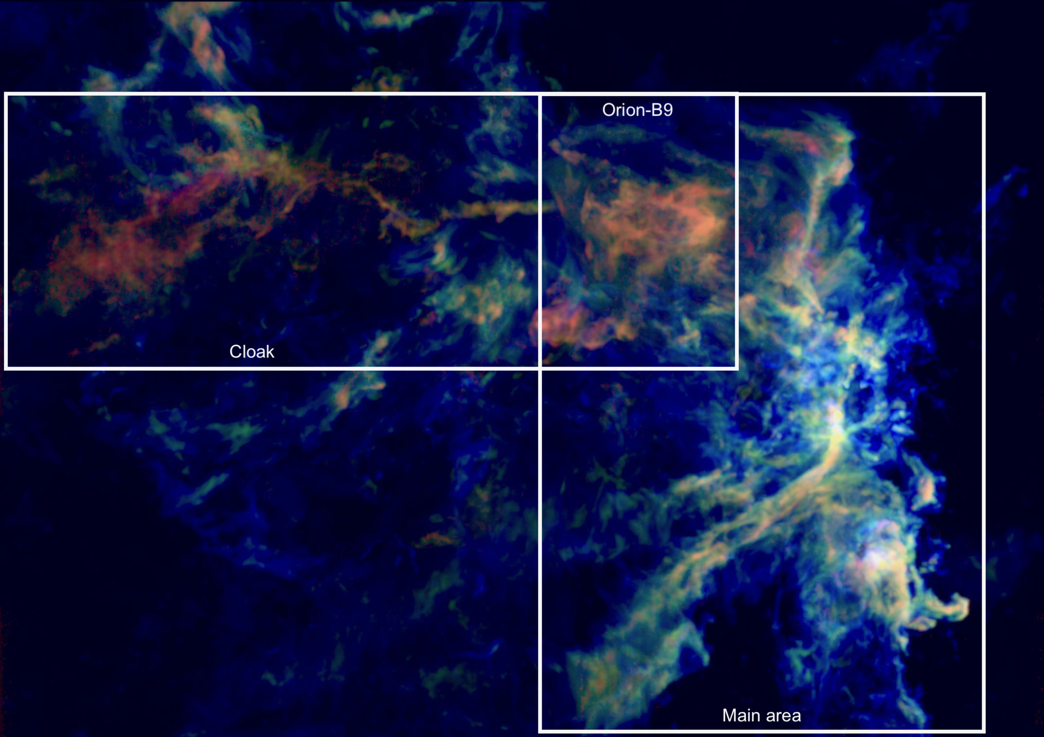
Figure 1: Carbon monoxide emission in the Orion B cloud. The image combines the peak temperatures of ¹²CO (1$-$0), ¹³CO (1$-$0) and C¹⁸O (1$-$0) coded in blue, green and red, respectively.

Observations reveal the ubiquitous presence of filamentary structures in molecular clouds, which play a fundamental role in the star formation process (André et al., 2010; Molinari et al., 2010; Palmeirim et al., 2013; Könyves et al., 2015). Indeed, pre-stellar cores and protostars mainly form in supercritical filaments (linear mass $M_{\mathrm{line}}>M_{\mathrm{line,crit}}=2c_{S}^{2}/G$), which are expected to be gravitationally unstable and, thus, the site of self-gravitational fragmentation (André et al., 2010; Tafalla & Hacar, 2015).

The angular momentum of a core is expected to be inherited from the initial core formation conditions.Historical studies (Goodman et al., 1993; Caselli et al., 2002) showed that the observed mean angular momentum within pre-stellar cores depends on their spatial scale. The gradients observed from single-dish mapping at $r>$3000 au have been interpreted as rotation and used to quantify the amplitude of the angular momentum problem for star formation and the expected disk radii around protostellar embryos. However, recent studies suggest that this trend could be due to pure turbulence motions or gravitationally driven turbulence (Tatematsu et al., 2016; Pineda et al., 2019; Gaudel et al., 2020). This in turn suggests that the connection between cores and the molecular cloud may be still present in the inner envelopes of young Class 0 protostars ($\sim$1600 au; Gaudel et al. 2020). Hence, the analysis of the gas dynamics in filaments could shed light on the origin of the angular momentum of the cores within them.

From molecular line observations, we know that filamentary structures exhibit complex motions with longitudinal collapse along the main filament (Kirk et al., 2013; Fernández-López et al., 2014; Tackenberg et al., 2014; Gong et al., 2018; Dutta et al., 2018; Lu et al., 2018; Chen et al., 2020) and radial contractions (Kirk et al., 2013; Fernández-López et al., 2014; Dhabal et al., 2018). Several studies have also highlighted velocity gradients perpendicular to the main filament, which suggests that the material may be accreting along perpendicular, low-density striations into the main filaments (Palmeirim et al., 2013; Dhabal et al., 2018; Arzoumanian et al., 2018; Shimajiri et al., 2019). While the filaments seem to accrete radially from their surroundings, the longitudinal collapse feeds central hubs or clumps, namely sites where the filaments converge (Myers, 2009; Schneider et al., 2010; Sugitani et al., 2011; Peretto et al., 2014; Rayner et al., 2017; Baug et al., 2018; Treviño-Morales et al., 2019).

Moreover, young massive stars are expected to have a strong impact on the surrounding environment, in particular by generating expanding H ii regions driven by UV ionizing radiation and stellar winds (Pabst et al., 2019, 2020). From a theoretical point of view, the ionization feedback from H ii regions would modify the properties of the molecular cloud, such as turbulence (Menon et al., 2020). From an observational point of view, the impact of young high-mass stars on future star formation properties is still poorly constrained. Several observational studies identified direct signatures of star formation, namely jets and outflows, at the edge of the H ii regions, suggesting that star formation could be triggered by the global effects of ionizing radiation and stellar winds (Sugitani et al., 2002; Billot et al., 2010; Smith et al., 2010; Chauhan et al., 2011; Reiter & Smith, 2013; Roccatagliata et al., 2013). Using high-angular-resolution ALMA (Atacama Large Millimeter/submillimeter Array) observations of the 1.3 mm continuum emission in eight candidate high-mass starless clumps, Zhang et al. (2021) suggest that H ii regions modify the dense material distribution around them, which tends to assist the fragmentation and, thus, the formation of future stars. However, there is no direct study of the kinematics around filamentary structures close to H ii regions to quantify their feedback effect on the filament formation and, thus, on star formation.

Understanding the initial properties of star-forming material and how they affect the star formation process is key. It is therefore crucial to robustly identify the physical mechanisms active in molecular clouds (turbulence, gravitational collapse, and magnetic fields) by analyzing the kinematics at different scales around the filamentary structures.

2 The ORION-B large program

The Outstanding Radio-Imaging of OrioN B (ORION-B) IRAM (Institut de Radioastronomie Millimétrique) large program (co-PIs: J. Pety and M. Gerin) is a survey of the southern part (five square degrees) of the Orion B molecular cloud, carried out with the IRAM 30-meter telescope (30m) at a wavelength of 3 mm.

Orion B, also known as the L1630 cloud, is located at a distance of $\sim$400 pc (Menten et al., 2007; Zucker et al., 2019) in the Orion Giant Molecular Cloud complex (Kramer et al., 1996; Ripple et al., 2013), east of the Orion Belt. Close to us, Orion B is a perfect object of study to fully understand stellar formation. This region is a active star-forming region: Könyves et al. (2020) identified thousand of dense cores closely associated with highly filamentary structures of matter from Herschel Gould Belt Survey (HGBS) observations. The Orion B cloud hosts several OB stars and well studied areas such as the Horsehead pillar (Zhou et al., 1993; Bally et al., 2018) and the associated photodissociation region (Goicoechea et al., 2009; Guzmán et al., 2013), the NGC 2023 and NGC 2024 star-forming regions, and the Flame and the Hummingbird filaments. Thus, it is a perfect target to study the kinematics around filamentary structures and the influence of feedback from massive OB stars on it.

The ORION-B program allows us to study in detail the properties of the molecular gas in the Orion B cloud such as the relationships between line intensities and the total gas column density (Pety et al., 2017; Gratier et al., 2017, 2021; Roueff et al., 2021), the structure of the different physical and chemical environments (Bron et al., 2018, 2021) and the characterization of turbulence modes (Orkisz et al., 2017). The main goals of this large observing program are to establish Orion B cloud as a local template for interpreting Galactic and extra-galactic molecular line observations (Pety et al., 2017). The Orion B cloud also hosts a large statistical sample of star-forming cores, which allows us to better understand star formation. In a previous work, Orkisz et al. (2019) developed a tool to identify and characterize the filament population in the southwestern part the Orion B cloud including NGC 2023 and NGC 2024. This paper presents an analysis of the kinematics around filaments in the ORION-B field of view, which contains the NGC 2023 - NGC 2024 complexes, the Orion B9 and the Cloak areas (see Fig. 1).

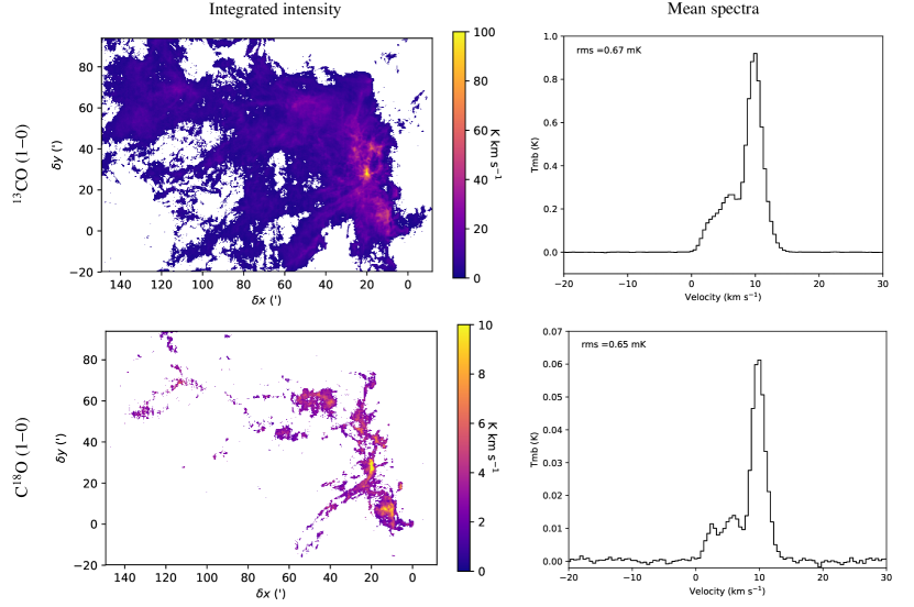
Figure 2: Zero-order moment maps (integrated intensity) of the total emission of the Orion B cloud (left) and mean spectra (right) of the ¹³CO (1$-$0) (top) and C¹⁸O (1$-$0) (bottom) molecular lines from the 30m data sets. For the zero-order moment map, the integration was done on a velocity range between -5 and 20 $\mathrm{\,km\,s^{-1}}$. Isolated pixels and pixels with a signal-to-noise ratio lower than 3 are blanked.

Table 1: Properties of the 30m datasets.

Line	Rest frequency	Resolution	Beam	Noise
	(GHz)	(km.s-1)	($\arcsec$)	(mK)
C18O (1$-$0)	109.782173	0.5	23.6	162
13CO (1$-$0)	110.201354	0.5	23.5	164

3 Observations and data set reduction

The observations were obtained at the IRAM 30-meter telescope (hereafter 30m) using the heterodyne Eight MIxer Receiver (EMIR) in one atmospheric windows E090 band at 3 mm (Carter et al., 2012) from 84.5 to 115.5 GHz. The Fast Fourier Transform Spectrometer (FTS) was connected to the EMIR receiver. The FTS200 backend provided total bandwidth of $\sim$32 GHz with a spectral resolution of 195 kHz (0.5 km s^-1). The full field of view of 5 square degrees was covered using rectangular tiles with a position angle of 14^∘ in the Equatorial J2000 frame to follow the global morphology of the Orion B cloud. Details of the observation strategy can be found in Pety et al. (2017).

Data reduction was carried out using CLASS, which is part of the GILDAS software, following the standard steps: removal of atmospheric emission, gain calibration, baseline subtraction, and gridding of individual spectra to produce regularly sampled maps with pixels of 9$\arcsec$ size. Details of each step can be found in Pety et al. (2017). Each datacube covers a velocity range of 120 km s^-1 (240 channels spaced by 0.5 km s^-1) centered at the rest line frequency (see Table 1). The spatial coordinates of the data cubes are centered onto the photon-dominated region (PDR) of the Horsehead Nebula at the coordinates (05h40m54.270s, -02^∘28$\arcmin$00.00$\arcsec$) and rotated by an angle of 14^∘ counterclockwise with respect to the Equatorial J2000 frame. The properties of the resulting maps, including the spatial resolution of the molecular line emission maps and the root mean square (rms) noise levels from the mean spectra are reported in Table 1.

4 Gaussian decomposition

From the mean spectra of the C¹⁸O and ¹³CO (1$-$0) molecular lines reported in Fig. 2, we identified several velocity components that seemed to belong to different layers of the Orion B cloud along the line of sight. To robustly investigate the kinematics, we need first to disentangle the different layers of the cloud. To do this, we used the Gaussian decomposition algorithm Regularized Optimization for Hyper-Spectral Analysis (ROHSA) developed by Marchal et al. (2019). This algorithm, based on a multi-resolution process from coarse to fine grid, uses a regularized non-linear least-square criterion to take into account the spatial coherence of the emission. This allows us to follow each Gaussian velocity component in the field of view, even at the transitions between spatial areas where the number of velocity components changes. In ROHSA, the model used to fit the data is a sum of Gaussians, where each Gaussian is parametrized by an amplitude $A_{i}$, a centroid velocity $\mu_{i}$ and a velocity dispersion $\sigma_{i}$. ROHSA takes as free parameters the number $N$ of Gaussian components, three hyper-parameters ($\lambda_{\mathrm{A}}$, $\lambda_{\mathrm{\mu}}$, $\lambda_{\mathrm{\sigma}}$) ensuring the spatial correlation of the model parameter maps for neighboring pixels, and $\lambda^{\prime}_{\mathrm{\sigma}}$ the variance of the velocity dispersion maps (Marchal et al., 2019). Using the parameter maps, we can reconstruct a de-noised signal with either the sum of all components defined as $\Sigma_{i}A_{i}\exp({-(\mathrm{v}-\mu_{i})^{2}/(2\sigma_{i}^{2})})$, or with a single component.

A visual inspection allows us to identify at least three velocity components in the C¹⁸O and ¹³CO mean spectra (see Fig. 2). However, non-Gaussian effects, such as line saturation, line wings, or velocity component asymmetry, must be taken into account by adding more Gaussian components than can be seen by a visual inspection to best reproduce the spectrum. We note that each emission line may trace different regions of the cloud (see Fig. 2), and hence the C¹⁸O and ¹³CO signals may not require the same number of Gaussian components to be reconstructed by ROHSA. To deduce the best total number of Gaussian components for each tracer, we initialized the algorithm to decompose the signal with several numbers $N=[3,4,5,6]$ of Gaussian components using an initial value $\sigma_{\mathrm{init}}=1.5\mathrm{\,km\,s^{-1}}$ for C¹⁸O and ¹³CO. The details of the different decompositions (residuals, $\chi^{2}$, velocity and velocity dispersion histograms) are given in Appendix A. Based on a trade-off between $\chi^{2}$ minimization and minimizing the number of components, the best total number of Gaussian components $N_{\mathrm{best}}$ is four and five to reconstruct the C¹⁸O and the ¹³CO (1$-$0) signals, respectively.

To find the best hyper-parameters, we also tried several values ($\lambda_{\mathrm{i}}=[10,100,1000],$ $\lambda^{\prime}_{\mathrm{\sigma}}=[0,1]$) for a given number $N$ of Gaussian components (see Appendix A). We selected $\lambda_{\mathrm{i}}$=100 for each hyper-parameter. The variance of the velocity dispersion maps $\lambda^{\prime}_{\mathrm{\sigma}}$ is set to zero to let free the variation of the velocity dispersion differences throughout the full field of view.

5 Identification and characteristics of the different velocity layers of the Orion B cloud

5.1 Moment maps

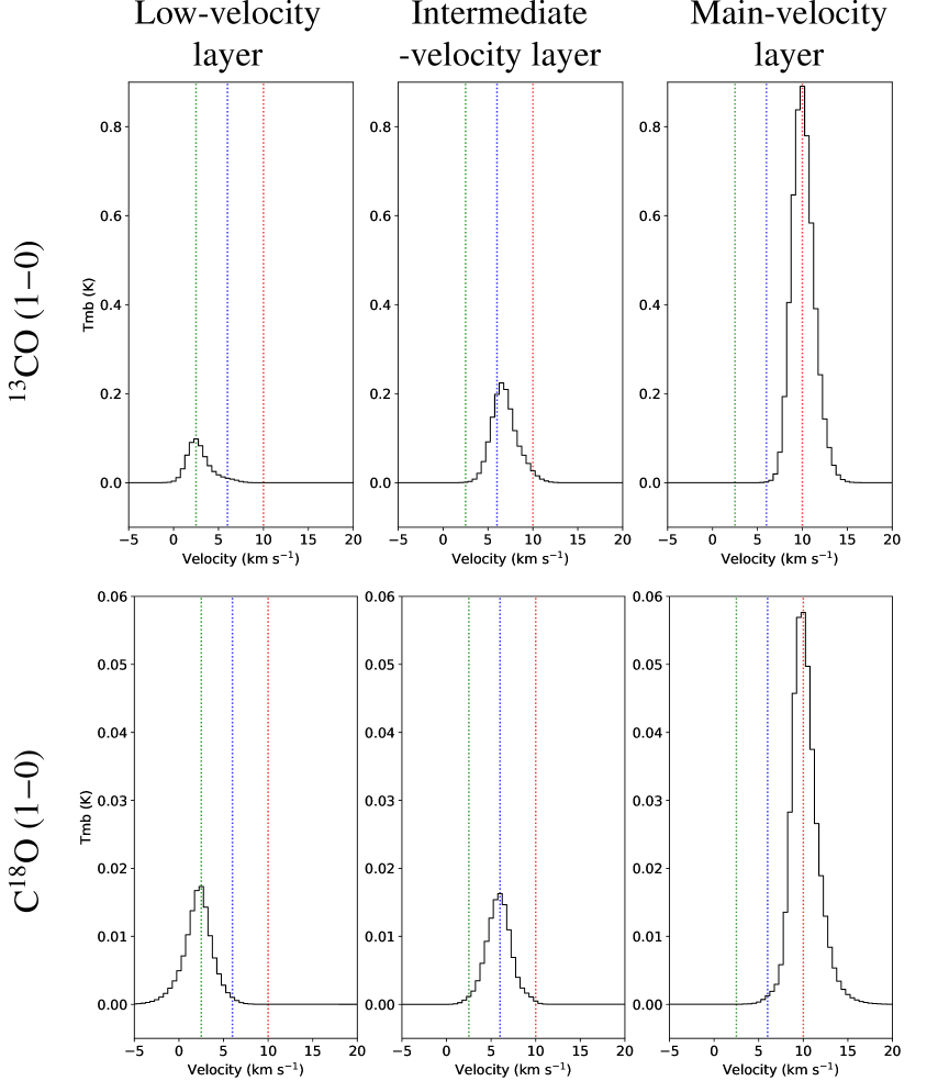
Figure 3: Mean spectra of the three layers of the Orion B cloud, namely the low-velocity layer (left), the intermediate-velocity layer (middle), and the main-velocity layer (right), from the ¹³CO (1$-$0) (top) and C¹⁸O (1$-$0) (bottom) emission rebuilt by ROHSA. The color dotted lines show the systemic LSR velocity of the three cloud layers.

Figure 4: Zero-order (integrated intensity, top), first-order (mean velocity, middle), and second-order (velocity dispersion, bottom) moment maps of each of the identified layer of the Orion B cloud, namely the low-velocity layer (left), the intermediate-velocity layer (middle), and the main-velocity layer (right), from the ¹³CO (1$-$0) (top) and C¹⁸O (1$-$0) (bottom) emission reconstructed by ROHSA. Isolated pixels, pixels with a signal-to-noise ratio lower than 3, and pixels with a mean velocity error higher than 0.25 km s^-1 are blanked.

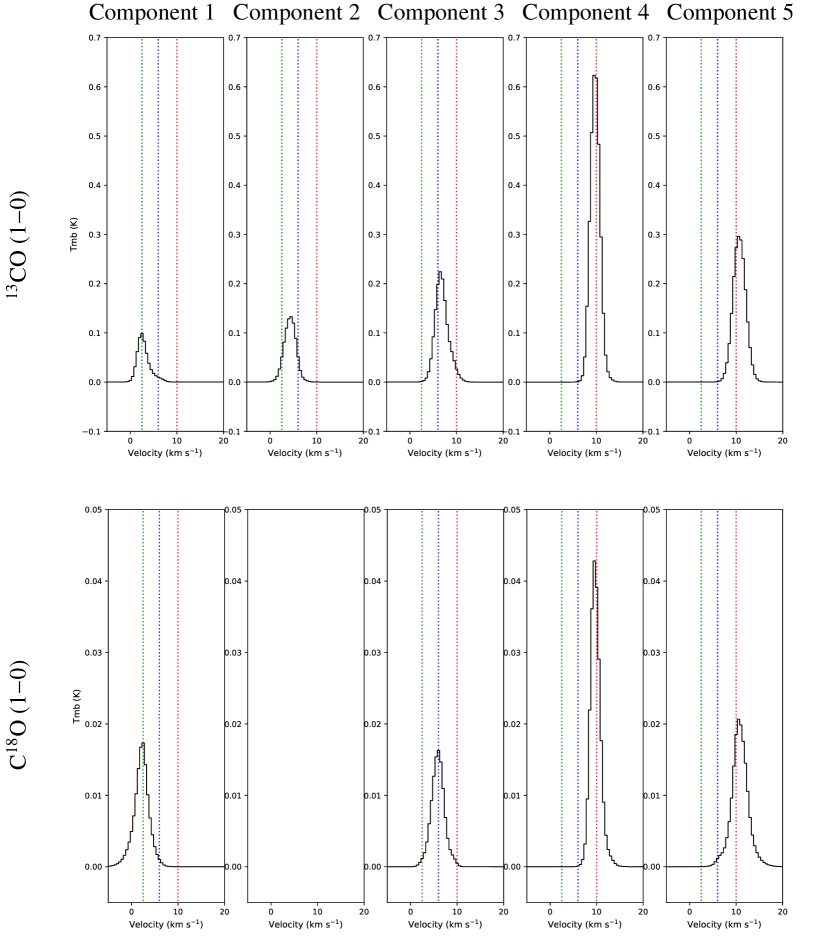
Figure 15: Mean spectrum of each Gaussian component fit by ROHSA for the ¹³CO (1$-$0) (top) and C¹⁸O (bottom) (1$-$0) line. The color dotted lines show the systemic velocity of the three cloud layers.

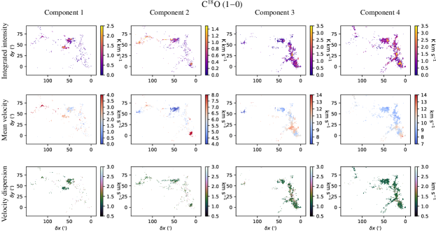
Figure 16: Zero-order (integrated intensity, top), first-order (mean velocity, middle), and second-order (velocity dispersion, bottom) moment maps of each of the four Gaussian components fit by ROHSA for the C¹⁸O (1$-$0) line. Isolated pixels and pixels with a signal-to-noise ratio lower than 3 are blanked.

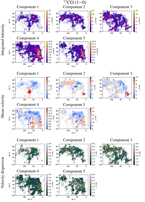
Figure 17: Zero-order (integrated intensity, top), first-order (mean velocity, middle), and second-order (velocity dispersion, bottom) moment maps of each of the five Gaussian components fit by ROHSA for the ¹³CO (1$-$0) line. Isolated pixels and pixels with a signal-to-noise ratio lower than 3 are blanked.

We built the zero-order (integrated intensity), the first-order (mean velocity) and the second-order (velocity dispersion) moment maps of each Gaussian component fit by ROHSA for the C¹⁸O and ¹³CO (1$-$0) lines (see Appendix B). We integrated each de-noised spectrum rebuilt by ROHSA on the velocity range $[-5,+20\mathrm{\,km\,s^{-1}}]$. Because of the spatial coherence, ROHSA can detect the Gaussian components up to a low signal-to-noise ratio (S/N $\lesssim$1$\sigma$). When including low S/N pixels, the amplitude and the width of the average spectrum inferred with ROHSA are larger than those of the average spectrum from the original data set. To avoid this effect, we only kept the pixels initially robustly detected, namely a spectrum detected with a signal-to-noise ratio higher than 3 in the initial data sets, to build the moment maps inferred with ROHSA. Figures 15-17 show the mean spectrum and the moment maps for each Gaussian components estimated for the two tracers.

On these moment maps, we observe that some Gaussian components trace the same spatial structures in the same velocity range and with a similar velocity dispersion. Given the close velocity ranges with respect to the velocity dispersion, the similarities in the structure of the integrated intensities from the C¹⁸O (1$-$0) moment maps (see Fig. 16), we identified the two last Gaussian components as coming from the same layer of the Orion B cloud. We added them together to recover the total signal of this cloud layer, which is not purely Gaussian. Three layers stood out (ordered by increasing systemic local standard of rest velocity): (i) the low-velocity layer with a systemic velocity around 2.5 kms^-1, (ii) the intermediate-velocity layer with a systemic velocity around 6 km s^-1, and (iii) the main-velocity layer of the Orion B cloud with a systemic velocity around 10 km s^-1.

In the following, we call these three layers the ”cloud” layers to differentiate them from the ”ROHSA” Gaussian components. From the ¹³CO (1$-$0) moment maps (see Fig. 17), the last two Gaussian components trace the main-velocity layer: as previously with the C¹⁸O data set, we added them together to recover the total signal of the layer. The first and the third Gaussian components trace the low and intermediate-velocity layers, respectively.

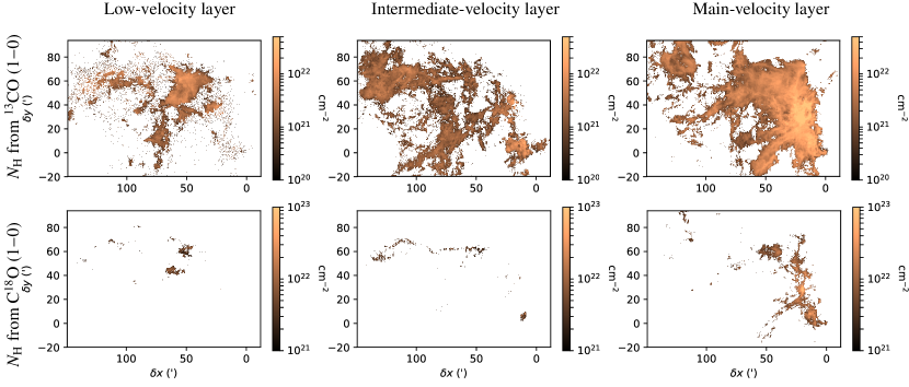
Figure 5: $N_{\mathrm{H}}$ maps of each of the identified layer of the Orion B cloud, namely the low-velocity layer (left), the intermediate-velocity layer (middle), and the main-velocity layer (right), from the ¹³CO (1$-$0) (top) and C¹⁸O (1$-$0) (bottom) emission reconstructed by ROHSA. Isolated pixels, pixels with a signal-to-noise ratio lower than 3, and pixels with a mean velocity error higher than 0.25 km s^-1 are blanked.

Figures 3 and 4 show the mean spectrum and the moment maps from the C¹⁸O and ¹³CO emission rebuilt by ROHSA for each identified layer of the cloud. From the zeroth-order moment maps, we observe that ¹³CO (1$-$0) traces more diffuse and more extended gas than C¹⁸O (1$-$0), which traces moderately dense gas (n_H $\gtrsim$ 10⁴ cm^-3). The cloud layers we identified above are velocity layers, but they may be located at different distances along the line of sight. In the Gaia Collaboration (2018) catalog, we identified young stellar objects (YSOs) with ages of less than 4 Myr located in the ORION-B field of view and with mean radial velocities corresponding to the velocity range of each cloud layer we identified. Young stellar objects are of interest because they are drifting slowly from their parent cloud and are still located within the boundaries of their parent cloud (Gaia Collaboration, 2018). The selected YSOs are all located at the same distance of $\sim$300-500 pc as the Orion B cloud showing that these velocity layers are associated with the Orion Complex. In this paper, we study the translucent medium (2 $\leq$ A${}_{\mathrm{V}}<$ 6 mag) and the moderately dense gas around the filamentary structures (6 $\leq$ A${}_{\mathrm{V}}<$ 15 mag) in the Orion B cloud, and thus we did not consider the low density turbulent medium (1 $\leq$ A${}_{\mathrm{V}}<$ 2 mag), which may connect these cloud layers. For example, we note that we need a fifth Gaussian component to recover the ¹³CO (1$-$0) signal, which traces more diffuse gas compared to C¹⁸O (1$-$0). This Gaussian component seems to trace the transition between the low-velocity and the intermediate-velocity layers with a systemic velocity around 4$\mathrm{\,km\,s^{-1}}$ (see component 2 in Figs. 15 and 17). In the following, we did not use this Gaussian component to analyze the kinematics of the cloud. This component represents only $\lesssim$25% of the total flux; thus, removing it has little impact on the analysis on the kinematics of the translucent and moderately dense gas.

In the low-velocity layer first-order moment maps in ¹³CO (1$-$0) (see Fig. 4), we notice a structure in the center-south. With a velocity higher than the rest of the layer, it seems not to be connected to this layer. Even if the nature of this structure remains unclear, it may correspond to a cloud located along the line of sight but at a different distance from Orion B. With a systemic velocity close to that of the low-velocity layer, the structure could be responsible for the line wing observed in the ¹³CO (1$-$0) mean spectrum of the layer (see Fig. 3). The weak intensity of the structure does not allow ROHSA to separate it from the low-velocity layer.

The spatial coherence of the velocity components extracted in the ROHSA decomposition in a way that allows continuous variations of the line parameters, as described in Marchal et al. (2019). The maps of the integrated intensity, mean velocity and velocity dispersion of each velocity component shown in Fig. 4 indeed exhibit spatial variations of these parameters, tracing the internal structure and dynamics of the three layers. For each velocity layer, the ROHSA decomposition has clearly captured the existing systematic intensity and velocity gradients.

5.2 Column density maps

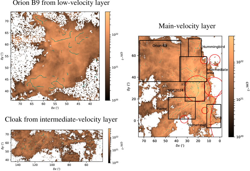
Figure 6: Subregions of interest overlaid on the $N_{\mathrm{H}}^{13}$ maps of each of the identified layer of the Orion B cloud, namely the low-velocity layer (top left), the intermediate-velocity layer (bottom left), and the main-velocity layer (right), from the ¹³CO (1$-$0) emission reconstructed by ROHSA. The green lines show the filamentary structures extracted from the C¹⁸O (1$-$0) emission. The red circles show the typical extensions of the H ii regions associated to massive stars (see Table 3).

From the C¹⁸O and ¹³CO (1$-$0) zero-order moment maps (see Fig. 4), we derived the column density $N_{\mathrm{H}}$ maps of each cloud layer by using the following equations (Orkisz et al., 2019; Roueff et al., 2021):

$$\begin{gathered}N_{\mathrm{C^{18}O}}/N_{\mathrm{H}}=\frac{5.6\times 10^{-7}}{2},\\ N_{\mathrm{{}^{13}CO}}/N_{\mathrm{H}}=\frac{2.5\times 10^{-6}}{2}.\end{gathered}$$ (1)

In these equations, $N_{\mathrm{H}}$ represents the total column of hydrogen, including the contributions of atomic and molecular hydrogen, $N_{\mathrm{H}}=N(\mathrm{HI})+2N(\mathrm{H_{2}})$. We assumed local thermodynamic equilibrium and an optically thin emission. We used the standard equations described in Mangum & Shirley (2015), the parameters values from the Cologne Database for Molecular Spectroscopy (CDMS; Endres et al. 2016), and the dust temperature $T_{\mathrm{dust}}$ map from Lombardi et al. (2014). We assumed that the dust temperature is a good estimate for the excitation temperature of ¹³CO (1$-$0) and C¹⁸O (1$-$0). The Orion B cloud layers we identified are not distinguished by Lombardi et al. (2014): the $T_{\mathrm{dust}}$ map is therefore the same for all cloud layers. More details on the assumptions made to compute the column density can be found in Sect. 2.4 of Orkisz et al. (2019). Figure 5 shows the column density maps of each layer of the cloud deduced from the ¹³CO (1$-$0) and C¹⁸O (1$-$0) data sets. In the following, we distinguish the column density deduced from the ¹³CO (1$-$0) and from the C¹⁸O (1$-$0) data sets with the notation $N_{\mathrm{H}}^{13}$ and $N_{\mathrm{H}}^{18}$, respectively. For the C¹⁸O (1$-$0) emission, we only kept the pixels with a column density $N_{\mathrm{H}}^{18}$ higher than 10²¹ cm^-2 because at lower values, the signal to noise ratio becomes marginal. For the ¹³CO (1$-$0) emission, we only kept the pixels with a column density $N_{\mathrm{H}}^{13}$ higher than 10²⁰ cm^-2. The highest contour of $N_{\mathrm{H}}^{13}$, 2.5 $\times$ 10²² cm^-2, spatially encompasses regions with even higher hydrogen column densities determined using the C¹⁸O (1-0) line. Thus, the ¹³CO and C¹⁸O molecules are complementary tracers of the kinematics. ¹³CO (1$-$0) becomes partially optically thick at high $N_{\mathrm{H}}$ (Roueff et al., 2021), so in the following we used the C¹⁸O data set to probe the kinematics robustly at high $N_{\mathrm{H}}$.

5.3 Error bars

The ROHSA algorithm does not provide the error bars of the output parameters (amplitude, centroid velocity and velocity dispersion) of the Gaussian components. Thus, we used the Monte Carlo method to estimate the error bars on the $N_{\mathrm{H}}^{18}$, on the $N_{\mathrm{H}}^{13}$ and on the centroid velocity maps of each cloud layer. We added a random Gaussian noise on each noiseless spectrum (i.e., each pixel) of each Gaussian component fit by ROHSA. The standard deviation $\sigma$ of the noise was chosen so that each individual spectrum (i.e., at each pixel) of the total signal rebuilt by ROHSA, namely the sum of all the Gaussian components, has a noise consistent with the one observed in the individual spectrum from the original data set.

From the randomly noised Gaussian components, we rebuilt the signal of each cloud layer and estimated the $N_{\mathrm{H}}^{18}$, the $N_{\mathrm{H}}^{13}$ and the first-order moment maps by selecting only the velocity channels with a signal-to-noise ratio higher than 3. We generated 1000 realizations to estimate the mean and the standard deviation. The mean maps and the standard deviation maps are shown in Appendix C. The mean maps of $N_{\mathrm{H}}^{18}$, $N_{\mathrm{H}}^{13}$ and first-order moment of each cloud layer are consistent with the maps inferred by ROHSA. In order to study the kinematics in a robust way, we chose to keep the pixels in the velocity maps with a standard deviation smaller than a half of the velocity channel width ($<0.25\mathrm{\,km\,s^{-1}}$). We note that the main structure of each layer has small velocity error bars, that are always lower than the selected criterion of 0.25$\mathrm{\,km\,s^{-1}}$. This criterion allows us to exclude the pixels with faint and noisy emission.

6 Extraction of the filamentary network

Table 2: Properties of the H ii regions ionizing stars.

Star	Spectral type	R.A., DEC (J2000)	Offset	Distance	HII region	Radius⋆
		(h:m:s, ∘:$\arcmin$:$\arcsec$)	($\arcmin$, $\arcmin$)	(pc)		($\arcmin$)
$\sigma$Ori	O9.5V B	05 38 44.779, -02 36 00.12	(-33.35, 00.07)	387.5 $\pm$ 1.3	IC 434	42
HD 38087	B5V D	05 43 00.573 , -02 18 45.38	(32.87, 01.33)	169 $\pm$ 37	IC 435	3
HD 37903	B1.5V C	05 41 38.388, -02 15 32.48	(13.72, 09.42)	362 $\pm$ 35	NGC 2023	2.5
Alnitak	O9.7Ib+B0III C	05 40 45.527, -01 56 33.26	(05.49, 31.04)	294 $\pm$ 21		11
IRS2b	O8V-B2V	05 41 45.50, -01 54 28.7	(20.54, 29.43)	415	NGC 2024	12
V⋆ V901 Ori	B2V C	05 40 56.370, -01 30 25.857	(14.44, 55.99)	437 $\pm$ 11		3.5
HD 37674	B5V(n) C	05 40 13.539, -01 27 45.25	(4.69, 55.99)	425 $\pm$ 15		5

(1) Schaefer et al. (2016); (2) Gaia Collaboration (2016); (3) Anthony-Twarog (1982) ; (4) Hummel et al. (2013); (5) Gaia Collaboration (2018).

To identify and locate the filamentary structures precisely in the different layers of the Orion B cloud, we applied on the $N_{\mathrm{H}}^{18}$ map estimated from the C¹⁸O (1$-$0) emission an algorithm developed and described in details in Orkisz et al. (2019). The algorithm is performed in a multi-scale fashion by re-scaling the $N_{\mathrm{H}}^{18}$ map by an $arcsinh$ function before computing the Hessian matrix. Then, the local aspect ratio of the structures and the column density gradient is used to refine the ridge detection. The raw skeleton obtained by this algorithm was cleaned by following several steps (see Orkisz et al. 2019 for more details).

First, the skeleton geometry was analyzed to remove the very short filaments, namely with an aspect ratio lower than two. Thus, we only kept the filaments with a length longer than twice the typical filament width (i.e., $\sim 0.2\mathrm{\,pc}$, Arzoumanian et al. 2011; Orkisz et al. 2019).

Second, we took the widths of the filaments into account. We removed the filaments with an unresolved width, namely lower than the resolution of the data sets (i.e., $\sim 0.02\mathrm{\,pc}$). Excessively large filaments (i.e., $\gtrsim 0.28\mathrm{\,pc}$) are also removed because they are unstable.

Third, we analyzed the shape of the filaments by computing their mean curvature radius and comparing it to the width of the filament in order to remove the very curvy filaments (i.e., ratio between curvature radius and width $<1.5$) but keeping the large-scale loops.

Finally, we measured the relative contrast to determine how many times denser the filament is compared to its surrounding medium. We put a lower limit on the relative contrast at $\sim 0.5$.

Filaments are removed if they are rejected by more than one criterion. Figure 6 shows the cleaned skeleton overlaid on the $N_{\mathrm{H}}^{13}$ maps of each layer of the Orion B cloud. Some filamentary structures within the main-velocity layer, as in the Horsehead Nebula or in the Intermediate area, are at the edge of H ii regions created by the intense UV ionizing from massive stars at large scales (see Fig. 6 and Table 3). The radii of the circles drawn in Fig. 6 are determined according to the size of the H ii region emission either in H$\alpha$ or in radio continuum (Pety et al. 2017; e.g., Martín-Hernández et al. 2005 for NGC 2023 and NGC 2024 for example). Using the Heracles code as described in Tremblin et al. (2014) and knowing the parameters of the exciting stars, the age of the H ii region and the expansion velocity of the neutral shell beyond the ionization front can be computed. The NGC 2024 H ii region is predicted to exert the strongest radiative feedback effect (P. Tremblin, priv. comm.).

7 Kinematics

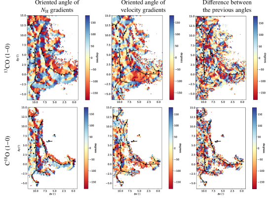
Figure 7: Maps of the column density gradient oriented angles (left) and the velocity gradient oriented angles (middle) in the Horsehead nebula from the main-velocity layer from the ¹³CO (1$-$0) (top) and the C¹⁸O (1$-$0) (bottom) emission. Right: maps of the relative orientation between the oriented angles of the column density and the velocity gradients. Oriented angles are defined north from east. The black lines show the filamentary structure and the diamond dots show the dense cores identified by the Herschel Gould Belt Survey (Könyves et al., 2020).

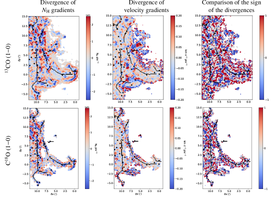
Figure 8: Divergence maps of the column density gradients in N_H pix^-1 (left) and the velocity gradients in km s^-1 pix^-1 (middle) in the Horsehead nebula from the main-velocity layer from the ¹³CO (1$-$0) (top) and the C¹⁸O (1$-$0) (bottom) emission. Right: comparison maps of the sign between the velocity gradient divergence and the column density gradient divergence. The values -1 (blue) or 1 (red) show the pixels where velocity and column density gradients both converge or both diverge. The value 0 (gray) indicates regions where the sign of at least one gradient is ill-defined because its modulus is close to zero. The black lines show the filamentary structure and the diamond dots show the dense cores identified by the Herschel Gould Belt Survey (Könyves et al., 2020).

7.1 Computation of velocity and column density gradients

From the first-order moment maps (see Fig. 4), we observe clear velocity patterns in the different layers of the Orion B cloud. In order to estimate the velocity gradients, we used the unbiased filter $[-1\,0\,1]/2$ in the horizontal and vertical directions, which means that, for a given pixel, we computed the difference between the velocity value at this pixel and the values at the pixels located forward and backward along the x- and the y-axis, and we divided by twice the pixel size. The pixels without forward or backward neighbors along the x- and y-axis are ignored. We determined the velocity gradients at each pixel for the different layers of the Orion B cloud. Using the same method, we determined the $N_{\mathrm{H}}^{13}$ and $N_{\mathrm{H}}^{18}$ gradients at each pixel. To facilitate the visualization of the gradients, we zoomed into different subregions of the cloud layers. Figure 6 shows the subregions of interest on the cloud layer $N_{\mathrm{H}}^{13}$ maps. Figure 7 shows as an example the maps of the oriented angle of the velocity and the column density gradients obtained for the main-velocity layer of the Horsehead Nebula. The oriented angle maps of the other subregions are provided in Appendix D.

As expected, we observe that in all subregions most of the filaments are located at the convergence of both $N_{\mathrm{H}}^{13}$ and $N_{\mathrm{H}}^{18}$ gradients, namely the gradients have opposite directions on both sides of the filaments. This is due to the filament extraction algorithm, which robustly detects the $N_{\mathrm{H}}^{18}$ ridges. Maps of $N_{\mathrm{H}}^{13}$ and $N_{\mathrm{H}}^{18}$ gradient oriented angles may be used as a simple way to detect the filamentary structures. We investigate the possible convergence of gradients in the following Sect. 7.2. Maps of the velocity gradient oriented angles show more complex patterns that are not easy to interpret from the maps. We investigate these results further in Sect. 7.3.

7.2 Convergence of the velocity and column density gradients

To quantify the possible convergence of gradients on localized areas, we calculated their 2D divergence using the following equation:

$$\mathrm{div}\leavevmode\nobreak\ \overrightarrow{\mathrm{grad}}=\frac{\partial\mathrm{grad}_{x}}{\partial x}+\frac{\partial\mathrm{grad}_{y}}{\partial y}.$$ (2)

When the value of the divergence is positive at a position, the gradients diverge from this same point, whereas the gradients converge to that point when the value is negative. Figure 8 shows as an example the divergence maps obtained for the main-velocity layer of the Horsehead Nebula. The divergence maps of the other subregions are provided in Appendix D. On these maps, we display the cores identified in the HGBS (Könyves et al., 2020). To select the self-gravitating objects, we only kept the objects identified as starless and pre-stellar cores with a Bonnor-Ebert mass ratio $<$2, combined with the cores that hosts confirmed YSOs. As Könyves et al. (2020) had no access to the cloud layers identified in this paper, the core selection is the same for all cloud layers.

A pattern of blue and red striations corresponding to convergence and divergence, respectively, of velocity and column density gradients, is visible. As expected from the oriented angle maps of the column density gradients, the filamentary structures in most subregions are located in convergence areas of both $N_{\mathrm{H}}^{13}$ and $N_{\mathrm{H}}^{18}$ gradients. The absolute values of the divergence of the gradient of $N_{\mathrm{H}}$ are larger along and near the filamentary structures in most subregions. In contrast, the filaments are mostly located in regions of low absolute value of the divergence of the centroid velocity gradient. This behavior is present in most of the analyzed subregions: the Horsehead Nebula, the intermediate area, the flame filament, NGC 2024, and the Hummingbird filament (see Fig. 8 and Appendix D). It suggests that velocity gradients become more coherent in the vicinity of coherent structures (i.e., filaments). In optically thin conditions, centroid velocity increments, built from molecular line profiles, are related to the average along the line of sight of some of the shear components (Lis et al., 1996). A high absolute value of the divergence of centroid velocity gradients can thus be interpreted as a signature of shearing motions along the line of sight associated with the current pixel. The relatively low absolute value of the divergence of centroid velocity gradients near filaments could indicate less active shearing motions in these regions. Such an effect was previously discussed by, for example, Pety & Falgarone (2003), in the case of the L1512 dense core. The much wider field of view allows us to increase the number of probed regions.

Figure 8 compares the sign of the divergence from the velocity and the column density gradients obtained in the Horsehead Nebula in order to highlight whether gradients in column velocity and density converge and diverge at the same place. The comparison between both gradient divergence signs of the other subregions are provided in Appendix D. The convergence and the divergence areas do not systematically correspond between the column density and velocity gradient. In most subregions, the gradients have opposite behaviors: when one converges, the other gradient diverges.

In the different subregions, cores are statistically located mostly at the convergence of the $N_{\mathrm{H}}^{13}$ and $N_{\mathrm{H}}^{18}$ gradients but are generally equally distributed in the convergence and divergence areas from the velocity gradients.

7.3 Comparison between velocity and column density gradients

In order to identify patterns and obtain coherent information on the kinematics in such a wide field of view, we developed a statistical and reproducible method that we applied in different subregions of the cloud. We compared the orientation between the velocity gradients and the column density gradients that characterize the density structures of the cloud. We computed the relative orientation between the oriented angles of the two gradients at each pixel without taking into account their magnitude. The result of this operation is characterized by a polar histogram (see Fig. 9). We were inspired by the method of the histogram of relative orientations developed by Soler et al. (2013) and used in Planck Collaboration et al. (2016) that compares the relative orientation of the magnetic field with respect to the density structures. To identify any preferential orientation of the velocity field with respect to the density structures, we built this histogram for different column density thresholds. We kept only the histograms with enough pixels to build them, namely with small error bars ($<$0.0005). We chose five values of the threshold based on the visual extinction values estimated by Pety et al. (2017), representing diffuse gas ($10^{20}\mathrm{\,cm^{-2}}$ and $10^{21}\mathrm{\,cm^{-2}}$), translucent gas $(3.5\times 10^{21}\mathrm{\,cm^{-2}})$, the environment of filaments $(10^{22}\mathrm{\,cm^{-2}})$, and the dense cores $(2.5\times 10^{22}\mathrm{\,cm^{-2}})$. In the different subregions, the histograms peak around 0^∘ and/or 180^∘ for the ¹³CO and C¹⁸O data set. The peaks are wider and noisier for the maps using the C¹⁸O (1$-$0) data set because the histograms are built on a smaller number of pixels than those using the ¹³CO (1$-$0) data set.

To illustrate the impact of an error on the choice of the ROHSA parameters, we show in Appendix E some results of the polar histograms obtained from another decomposition, such as $\lambda_{\mathrm{i}}=10$. We see that there is very little difference with the results for the chosen decomposition. By selecting the pixels with a signal-to-noise ratio higher than 3 and with velocity error bars lower than $0.25\mathrm{\,km\,s^{-1}}$, we only kept the pixels with a robust kinematic signal. We obtained a robust estimation of the gradients by using forward or backward neighbors along the x- and y-axis for each pixel. The kinematic patterns highlighted in the histograms are therefore not due to the ROHSA decomposition or to random noise in the data sets but reflect the complexity of the kinematic motions of the gas in the Orion-B cloud.

In the histograms of NGC 2024, the Cloak, and the low-velocity layer associated with Orion B9, a change of pattern is visible between the histogram angles built from the ¹³CO(1$-$0) data set, and those using the C¹⁸O(1$-$0) one. In NGC 2024, the histogram peaks at 180^∘ in ¹³CO whereas in C¹⁸O, the histogram peaks at 0^∘. The ¹³CO and C¹⁸O emissions do not trace the gas from the same spatial area in NGC 2024: a more extended region is detected in ¹³CO (1$-$0) compared with the restricted area showing C¹⁸O (1$-$0) emission. Thus, this result suggests a change in the mechanisms responsible for the kinematics depending on the traced volume of gas. For Orion B9 from the low-velocity layer and the Cloak, the difference between the two lines can be explained by the low number of pixels available in the C¹⁸O data set, resulting in large error bars on the histograms. In the following, only the histograms from the ¹³CO emission for these two regions will be considered.

In all regions except the intermediate area, the shape of the polar histograms is relatively stable when increasing the column density threshold. In the intermediate area, the histograms peak at 180^∘ both in ¹³CO and in C¹⁸O at high column density, namely the dense core column density ($N_{\mathrm{H}}>$ 2.5 $\times$ 10²² cm^-2), whereas at lower column density thresholds, the histograms peak only at 0^∘. This suggests a change in the mechanisms responsible for the high column density gas kinematics in ¹³CO and in C¹⁸O as compared with the gas at a lower column density.

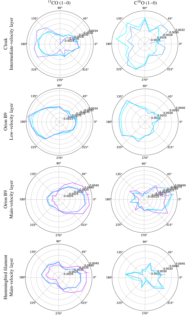
Figure 9: Polar histogram of the relative orientation between the oriented angles of the column density and the velocity gradients from the ¹³CO (1$-$0) (left) and the C¹⁸O (1$-$0) (right) emission for the different sub-regions of interest within the Orion B cloud. The different colors correspond to the column density thresholds. For ¹³CO (1$-$0): data with $\log(N_{\mathrm{H}}^{13})>20.00$ cm^-2 are shown in cyan, $\log(N_{\mathrm{H}}^{13})>21.00$ cm^-2 in blue, $\log(N_{\mathrm{H}}^{13})>21.55$ cm^-2 in blue-violet, $\log(N_{\mathrm{H}}^{13})>22.00$ cm^-2 in purple, and $\log(N_{\mathrm{H}}^{13})>22.40$ cm^-2 in fuchsia. For C¹⁸O (1$-$0): data with $\log(N_{\mathrm{H}}^{18})>21.00$ cm^-2 are shown in cyan, $\log(N_{\mathrm{H}}^{18})>21.55$ cm^-2 in blue, $\log(N_{\mathrm{H}}^{18})>22.00$ cm^-2 in purple, and $\log(N_{\mathrm{H}}^{18})>22.40$ cm^-2 in fuchsia. The colored bars at 10^∘ show the error bars of the histograms.

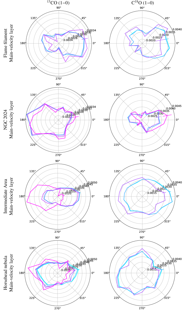
Figure 9: Continued.

8 Discussion

8.1 Physical processes that dominate the velocity field

To identify the physical mechanisms responsible for the patterns observed in the histograms, we created 3D toy models of the velocity and volume density fields around an isolated filament. After processing these models in the same way as the observed data, we produced polar histograms from the models which can be compared with those obtained from the observations. This allows us to distinguish two main behaviors of the kinematics around filaments: (i) velocity fields that mainly depend on the radial distance to the filament, such as a radial inflow or a radial outflow, and (ii) velocity fields along the main filament axis (i.e., longitudinal flows), where the velocity varies along the filament axis to promote the formation of a core (Hacar & Tafalla, 2011).

8.1.1 Results from toy models

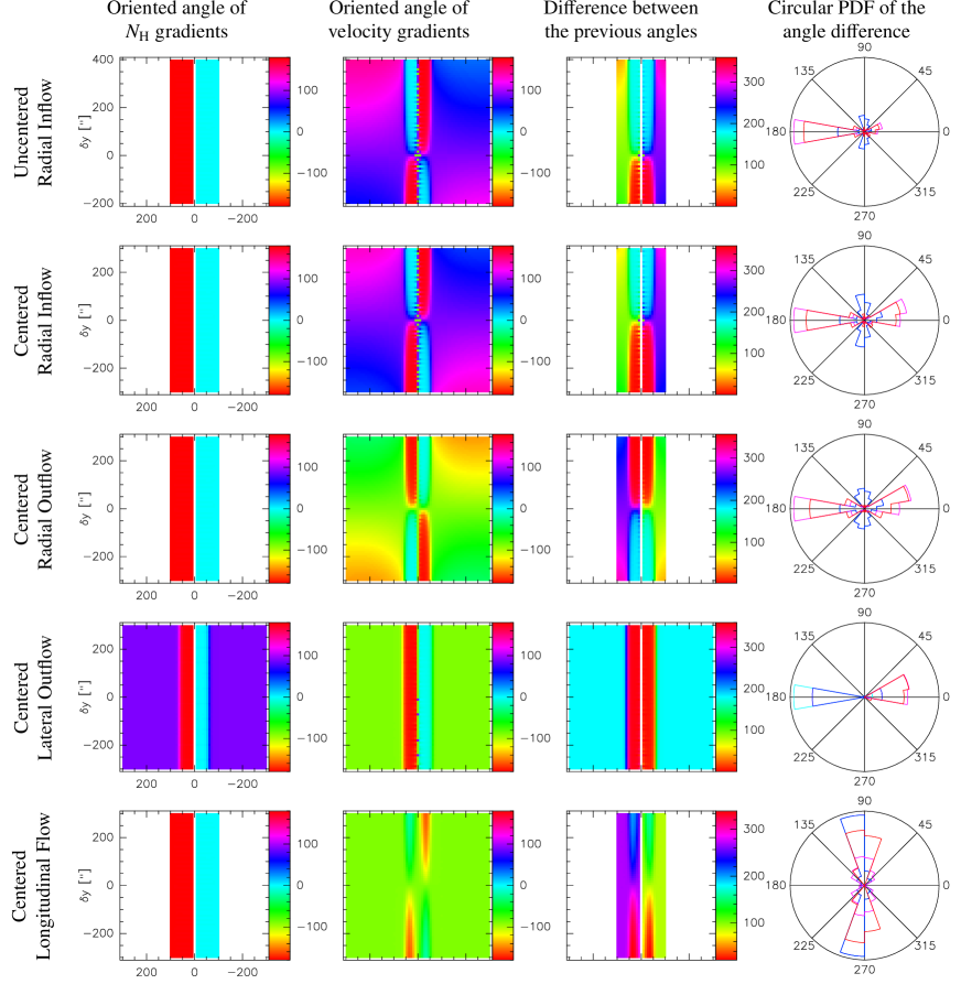
Figure 10: Oriented angles of the gradient of column density and centroid velocity, and their differences for five different toy models of the density and velocity fields. All angles are displayed in degree. The white areas on the images show regions where the gradient is too small to reliably compute its orientation. The different colors of the circular probability distribution function (PDF) correspond to the column density thresholds which are used in the Orion B data set analysis: $\log(N_{\mathrm{H}})>21.00$ cm^-2 are shown in cyan, $\log(N_{\mathrm{H}})>21.55$ cm^-2 in blue, $\log(N_{\mathrm{H}})>22.00$ cm^-2 in pink, and $\log(N_{\mathrm{H}})>22.40$ cm^-2 in red.

The models are here meant to represent simple geometric configurations. Hence, they only implement regular density and velocity fields, and do not include velocity fluctuations nor random motions due to turbulence for example. In the ORION-B observations, the filaments are located at the convergence of the column density gradients. We thus modelled the filament volume density with an infinite cylinder whose section follows a 2D Gaussian function. In order to explore the variety of kinematic behaviors, we considered four different patterns for the velocity field: three flows perpendicular to the filament axis, and a flow along the filament axis. In all cases, we used simple analytical formulae to describe the modulus of the velocity. The three flows perpendicular to the filament axis are (i) a gravitational inflow motion, (ii) an accelerated outflow motion, and (iii) a one sided flow. The latter flow is devised to model the filaments that are located at the edges of H ii regions (Pety et al. 2017; see Fig. 6). In this case, one side of the filament is ionized, and the kinematics information of the molecular gas is accessible only from the other side of the filament. The last model is intended to represent a core forming flow, along the main filament axis. Details of each model are given in Appendix F.

The cubes of volume density and velocity are then inclined by 30^∘ with respect to the plane of sky and integrated along the line of sight to compute the maps of column density and centroid velocity. We then computed their gradients, the associated oriented angles, and their differences. Figure 10 shows the histograms of the relative orientation between the gradients of column density and centroid velocity. Models where the flow is perpendicular to the filament axis show a preferred orientation of the polar histograms at 0^∘ and 180^∘. In contrast, the model with a longitudinal flow exhibits a pattern with peaks at 90^∘ and 270^∘. The difference between the patterns predicted for the studied inflow and outflow models is moderate. The lateral flow model shows the same 0^∘ – 180^∘ orientation but with a pronounced asymmetry with low column density contours on one side and high column density contours on the other side.

More generally, the symmetry between the histogram peaks located at $180^{\circ}$ from each other comes from the symmetry of the toy models. When the axis of inclination of the filament on the plane of sky is moved upward or downward along the filament axis, the histogram becomes asymmetrical : the amplitude of one of the peaks (for example the peak at 0^∘) becomes higher and that at of the other peak becomes lower.

8.1.2 Comparison between models and observations

A comparison of the modeled (Fig. 10) and observed (Fig. 9) histograms indicates that the models with a velocity field perpendicular to the main filament axis clearly reproduce the observations better. Indeed, the histograms built from the observed data show clear peaks at $0^{\circ}$ and/or $180^{\circ}$ rather than at other angles. In addition peaks at angles $90^{\circ}$ or $270^{\circ}$ that are expected in the case of a longitudinal velocity field are not detected in any of the studied regions.

By exhibiting a main peak at 0^∘ in their ¹³CO and C¹⁸O histograms, and a weaker secondary peak at 180^∘, the velocity fields of the Orion B9 area in the main-velocity layer and the Flame filament are consistent with a radial inflow on the filaments in the case when the projection center is not localized in the center of the studied field. The C¹⁸O histogram corresponding to the Hummingbird filament does not show any clear orientation due to the low number of pixels having a high S/N ratio C¹⁸O emission. The ¹³CO histogram shows two peaks at 0^∘ and $135-190^{\circ}$.We also notice that at high column density $(>10^{22}\mathrm{\,cm^{-2}})$, the second peak around 135^∘ is less pronounced than at lower column densities while the main peak increases. This histogram is not consistent with the radial inflow or outflow models when the center of symmetry is located in the middle of the filament because we expect two equivalent peaks at 0^∘ and 180^∘. With a clear main peak at 0^∘, the mechanism dominating the kinematics in the Hummingbird filament is radial inflow with a displacement of the center of projection. Depending on the orientation, a lateral flow would also be possible, reinforcing the diagnostic of a significant asymmetry.

By showing two equivalent peaks at 0^∘ and 180^∘ in their ¹³CO histograms, the velocity fields of the Horsehead Nebula, the Cloak, and the Orion B9 area from the low-velocity layer are consistent with the velocity field resulting from radial inflow or outflow motions. The Horsehead Nebula is at the edge of the H ii region, created by the O9 star $\sigma$Ori, whose expansion can exert a lateral pressure on the Horsehead Nebula, and inflowing and/or outflowing motions explaining the histogram with two peaks at 0^∘ and 180^∘ (see Fig. 6 and Table 3). Orion B9 (both layers) and the Cloak are located in a quiet region of the Orion B cloud without H ii region. However, their ¹³CO histograms from the low and intermediate-velocity layers also indicate the presence of an asymmetry and velocity fields perpendicular to the filament axes.

In NGC 2024, the different patterns of the ¹³CO and C¹⁸O histograms, which are both aligned along the 0^∘ – 180^∘ line but on opposite directions, indicate a strong asymmetry. This is consistent with the lateral flow model in the ionized case, a likely scenario because the IRS2b star in the center of the NGC 2024 region generates a dense H ii region, the expansion of which can push the molecular gas outward. The NGC 2024 region is also located at the edge of the H ii region created by the Alnitak star which can cause lateral pressure (see Fig. 6 and Table 3). As the ¹³CO emission traces the translucent gas in the cloud, it is differently affected by H ii regions than the gas in the filamentary structure traced by C¹⁸O. This explains the structure of the C¹⁸O histogram which shows a main peak at 0^∘ consistent with the effect of the expansion of the H ii region. In the intermediate area, the ¹³CO and C¹⁸O histograms peak at 180^∘ at the high column density threshold whereas they peak at 0^∘ at lower column density thresholds, a pattern associated with lateral flows. Indeed, at high column density, the gas traced by the ¹³CO and C¹⁸O emission corresponds to the filamentary structures located in the south of the intermediate area at the edge of the H ii region created by the IRS2b star in the center of the NGC 2024 region (see Fig. 6 and Table 3). Thus, the kinematics at high column density can be due to a lateral pressure on partially ionized filaments.

8.2 Star formation induced by H ii regions

Our study of selected regions in the ORION-B field of view shows the effect of H ii regions in driving the kinematics of the molecular gas and the formation of filamentary structures. A previous study done with the ¹³CO (1$-$0) emission by the ORION-B team (Orkisz et al., 2017) identified compressive modes of turbulence around the active star-forming regions NGC 2024 and NGC 2023, while the quieter regions, the Hummingbird and Flame filaments, exhibit mostly solenoidal motions. The southern part of the Intermediate region is also a highly compressive region while the northern part seems to be dominated by solenoidal motions. These two observational ORION-B studies put together are consistent with recent numerical simulations that suggest that H ii regions drive compressive motions in pillar-like structures, thus triggering star formation (Menon et al., 2020). This is also consistent with the conclusion of Bally et al. (2018). They studied the kinematics of the IC434 H ii region ionized by $\sigma$Ori, and the nearby Horsehead Nebula using SOFIA-GREAT observations of the [CII] 158$\mu$m line. They conclude that the ionization front induced a pressure shock triggering a compression of the western edge of the cloud. They also suggest that the compression would not only be due to $\sigma$Ori but also to older generations of massive stars.

The Horsehead Nebula is an active star-forming region. Two dense condensations were identified as dense cores in approximate gravitational equilibrium by Ward-Thompson et al. (2006). Bowler et al. (2009) found five candidate young stars, a class II YSO, and two protostars in this region. For the NGC 2024 region, maps of dust emission at 1 mm by Mezger et al. (1988, 1992) exhibit high-density condensations aligned in an elongated ridge running north to south, namely the filamentary structure we identified at the edge of the H ii region generated by Alnitak (see Fig. 6). Submillimeter and millimeter observations reveal outflows associated with some of the dense condensations in NGC 2024, which would therefore be young protostars (Moore & Yamashita, 1995; Richer, 1990; Richer et al., 1992). Choi et al. (2012) also detected H₂O and CH₃OH maser lines, which suggests that the NGC 2024 region is actively forming stars. The methanol masers suggest the existence of shocks that may be driven by YSOs outflows (Urquhart et al., 2015) or the expanding H ii regions.

Therefore, the NGC 2024 and NGC 2023 H ii regions could be good examples of the triggering effect of future star formation by exerting a lateral pressure that causes compressive motions, favoring the formation of filamentary structures at their edges and, thus, the formation of new stars. Hosokawa & Inutsuka (2006) studied the expansion of H ii regions and dissociation fronts due to a massive star performing numerical calculations of radiation-hydrodynamics. They conclude that the H ii region expands, accumulating molecular gas at the edge where gravitational fragmentation is then expected.

The compression phenomenon could probably also be reinforced by the photo-evaporation flow at the illuminated edges of molecular clouds. Indeed, the UV-illuminated gas at the ionization and dissociation fronts expands and exerts a compression on the molecular part of the cloud (Bertoldi, 1989; Bertoldi & Draine, 1996). Bron et al. (2018) and Joblin et al. (2018) recently model photo-evaporation flows from the illuminated edges of molecular clouds and find that they can induce high pressures that could explain the origin of the dense structures found at the edges of H ii regions. The presence of dust in the IC 434 H ii region and the kinematics of ionized carbon (Bally et al., 2018) indeed indicates the presence of an evaporation flow at the edge of the Horsehead Nebula.

8.3 Inflow due to gravitationally driven turbulence

In the absence of H ii regions, radial flows seem to be the main mechanism dominating the kinematics around filaments as the observed pattern are consistent with radial inflows or outflows toward the filament ridges. Radial inflows are more likely as they contribute to the accretion of material onto the filaments to increase their linear mass and bring them closer to the critical state for collapse. We have found a decrease of the amplitude of centroid velocity gradients divergence in the filaments, indicating a more coherent behavior of the velocity field in the filaments as compared with their surroundings, an expected behavior in the case accretion on filaments (Heigl et al., 2020). Such a velocity pattern could be due to different mechanisms, including pure infall induced by gravitational collapse, pure externally driven turbulence, gravitationally driven turbulence, or accretion flows channeled by magnetic field. Below, we discuss these four possibilities.

Low-density striations, which may be unresolved in our single-dish observations of the Orion B cloud, are usually observed perpendicular to filaments, suggesting that the cloud material is accreting along these striations onto the main filaments (Palmeirim et al., 2013; Dhabal et al., 2018; Arzoumanian et al., 2018; Shimajiri et al., 2019). Shimajiri et al. (2019) produce a toy accretion model and compare the modeled velocity patterns to those observed by Palmeirim et al. (2013) around the B211/B213 filament. They suggest that the gas is located in a thin shell at the edge of a super-bubble and that the radial accretion flow in this shell onto the filament is controlled by the gravitational potential of the filament. In this scenario, the inflow we observed in the Orion B cloud would be due to pure infall induced by gravitational collapse. From estimates of the effective gravitational instability criterion, Orkisz et al. (2019) identify super- or trans-critical filaments in the NGC 2024 region. In this region, the flow we observed in the moderately dense gas traced by the C¹⁸O (1$-$0) emission could be consistent with gravitational collapse motions. However, the other filaments would be subcritical structures, suggesting that they are not collapsing to form stars yet. Thus, the radial flows we identified in the Flame and Hummingbird filaments for example, would contribute to the accretion of matter on these young filaments to increase their linear mass and bring them closer to the critical state. In this case, the radial velocity flow might not be due to pure gravitational infall but could correspond to a combination of infall, compressive motions or accretion channels along the magnetic field.

Several filament formation scenarios support the fact that filaments are formed by an external turbulent compression (Smith et al., 2014, 2016) or the collision of two supersonic turbulent gas flows (Pety & Falgarone, 2000; Padoan et al., 2001; Tafalla & Hacar, 2015; Clarke et al., 2017). In this picture, the turbulent cascade generated initially could be responsible for the inflow observed around some of the filamentary structures in the Orion B cloud. The Orion B molecular cloud is highly supersonic with a mean Mach number between six and eight (Schneider et al., 2013; Orkisz et al., 2017). This high Mach number is usually interpreted as due to the turbulent cascade from the scale of molecular cloud (tens of pc) down to the scale of a filament (0.1 pc) (Kritsuk et al., 2013; Federrath, 2016; Padoan et al., 2016). However, some regions, as NGC 2024, the Flame and Hummingbird filaments, are moderately supersonic, with a Mach number between 3 and 5 (Orkisz et al., 2017). For the actively star-forming region NGC 2024, we could expect a lower Mach number if collapse motions were contributing significantly to the velocity field. Indeed, it is expected that the gravitational instability will convert potential energy into kinetic energy, and the associated shocks will contribute to the dissipation of a fraction of the turbulence. The decrease of the Mach number in dense filaments is also often interpreted as a sign of dissipation of turbulence (e.g., Orkisz et al., 2019) as this reduction is associated with a smaller velocity dispersion. For the Flame and Hummingbird filaments, the moderately supersonic Mach number as compared with the bulk of the cloud, also suggests that externally driven turbulence is not responsible for the radial flow motion. Further work is needed to determine the degrees of turbulent, thermal and magnetic support of the filaments and how they change with their evolutionary stage to confirm whether filaments with lower Mach number than the bulk of the gas indeed show infall motions.

The gravitational potential of the filaments could lead to radially dominated accretion and could generate turbulent motions at the same time. Numerical studies on gravitationally driven turbulence associated with accretion on filaments (i.e., neglecting the self-gravity of filaments) succeed in reproducing the linear relation between velocity dispersion, size, and subsonic inflow velocity (Ibáñez-Mejía et al., 2016; Heigl et al., 2018), which is usually expected to be due to pure turbulent motions. From these results, they argue that gravitationally driven turbulence due to the gravitational potential of the filaments is a significant source of turbulent motions. The velocity and velocity dispersion pattern predicted for self gravitating filaments by Heigl et al. (2020) (radial accretion, constant turbulent pressure) is consistent with the properties of the Flame filament. The inflow we observed in the Flame filament, and by extension in the Hummingbird filament and in the Orion B9 region, should be further studied as a test case of gravitationally driven turbulence around filaments.

Polarization observations revealed a change of the magnetic field direction with density: the magnetic field is parallel to the diffuse gas structures (Chapman et al., 2011; Palmeirim et al., 2013; Planck Collaboration et al., 2016) and becomes perpendicular to dense gas structures, especially the filamentary structures (Sugitani et al., 2011; Planck Collaboration et al., 2016). This change has been also observed in 3D and 2D models of magnetized molecular cloud formation (Seifried et al., 2020) and interpreted as due to compressive motions, which can be the result of gravitational collapse or converging flows along filamentary structures (Soler & Hennebelle, 2017). Shocks located along the filament edge is another possibility (Hu et al., 2019, 2020). Thus, the global magnetic field would be distorted by the gas becoming self-gravitating after flowing along the B field lines in low density diffuse regions (Heyer et al., 2016; Tritsis & Tassis, 2016; Chen et al., 2017). Low-density and thermally subcritical filaments, such as the perpendicular striations, are expected to be parallel to the magnetic field, while high-density and self-gravitating filaments should be preferentially oriented perpendicular to the field lines (Nagai et al., 1998). This may explain the distribution of filament orientations with two orthogonal groups found in several clouds (Peretto et al., 2012; Palmeirim et al., 2013; Cox et al., 2016; Ladjelate et al., 2020). The relative orientation of filaments with respect to the magnetic field is therefore an important element to fully understand their dynamical state. However, the Planck polarization data set does not have a sufficient angular resolution (2.5$\arcmin$) to estimate robustly the relative orientation of magnetic field with respect to the filaments we studied in the ORION-B field (Orkisz et al., 2019). Polarization measurements at higher angular resolution, reaching 0.1  pc or better, are thus required.

8.4 Longitudinal flows

Among the studied fields we have not found evidence for longitudinal flows as discussed by, for example, Hacar & Tafalla (2011) in the context of core formation within a filament. Because of the limited spatial resolution of the ORION-B data ($\sim 0.05$  pc, these phenomena may not contribute much to the statistics of the centroid velocity gradients as compared to the other types of flows that are more extended. Nevertheless, the toy models clearly indicate that the specific geometry of core forming flows can be clearly identified with the proposed method. Further studies at a higher linear resolution may therefore help in identifying these flows.

9 Conclusions

In the framework of the ORION-B program, we analyzed the kinematics around filamentary structures in the Orion B cloud. The main results of our study are listed below.

1. Using the ROHSA algorithm, we distinguished three cloud velocity layers at different systemic velocities (2.5, 6, and 10 km s^-1) in the translucent and moderately dense gas.

2. We identified the filamentary network of each velocity layer. The filaments are preferentially located in regions of low amplitude centroid velocity gradients.

3. By comparing the orientation of density column gradients and the orientation of velocity gradients from the ORION-B observations and synthetic observations from 3D toy models, we were able to identify the physical mechanisms at work around the filamentary structures. This simple statistical method can be reproduced in any molecular cloud to obtain coherent information on the kinematics. This allows us to distinguish two types of behavior in the kinematics around filaments: (i) a radial flow of the molecular matter toward the filament ridges and (ii) a longitudinal flow associated with the formation of a core within the filament.

4. H ii regions tend to generate compressive motions via an outflow or a lateral pressure on the translucent gas, favoring the formation of filamentary structures at their edges, in, for example, NGC 2024. This is the first observational study to highlight feedback from H ii regions on filament formation and, thus, on star formation in the Orion B cloud.

5. Without nearby H ii regions, radial inflow seems to be the main mechanism dominating the kinematics around the filaments (Hummingbird, Flame, and Orion B9 areas in the main-velocity layer) and may reveal the accretion processes generating gravitationally driven turbulence.

These results were obtained by observing molecular line data at high S/N, high spectral resolution, over a wide area encompassing more than two decades of spatial scales. The methods we developed could be applied to other molecular clouds to investigate the relationships of filaments with their parent molecular cloud in different environments and at different evolutionary stages.

Appendix A Comparison between the Gaussian decomposition parameters

A.1 Best total number of Gaussian components

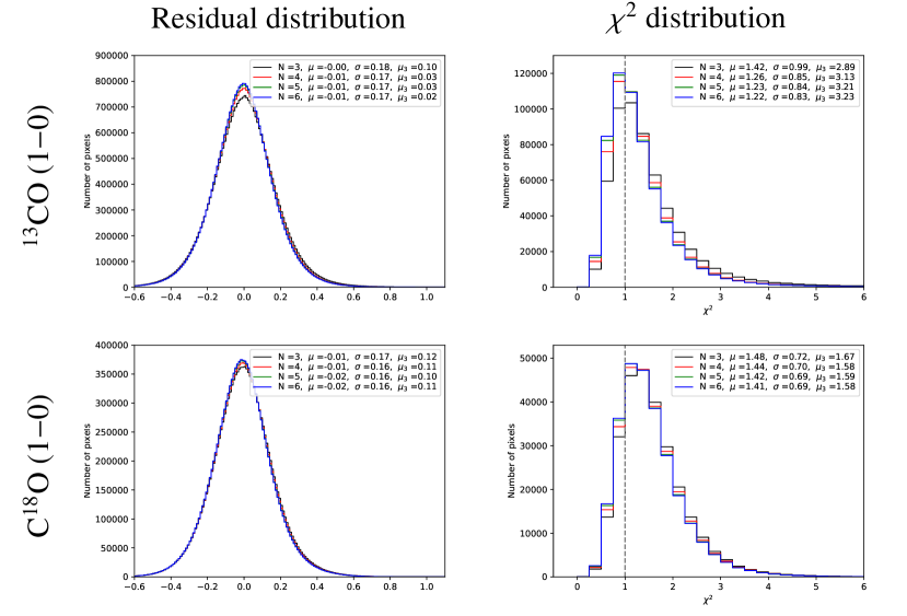
Figure 11: Residual (left) and $\chi^{2}$ (right) distributions between the original and the ROHSA reconstructed cubes for different numbers $N$ of Gaussian components and $\lambda_{\mathrm{i}}=100$ from the ¹³CO (1$-$0) (top) and C¹⁸O (1$-$0) (bottom) emission, respectively. The mean, variance and skewness of each distribution are shown in legend.

To identify the best total number of Gaussian components for C¹⁸O and ¹³CO, we initiated the ROHSA algorithm to decompose the signal with a series of Gaussian components with an initial velocity dispersion of $\sigma_{\mathrm{init}}=$1.5 km s^-1. We computed a decomposition with $N$ = [3, 4, 5, 6] Gaussian components for a given value of hyper-parameters ($\lambda_{\mathrm{i}}$=100, $\lambda^{\prime}_{\mathrm{\sigma}}$=0). For the different numbers of Gaussian components, we estimated the residuals between the original and the ROHSA reconstructed cubes, and computed the $\chi^{2}$ of the fit on each spectrum (i.e., at each pixel). We computed the $\chi^{2}$ on the velocity range -5 $-$ 20 km s^-1 following the equation

$$\chi^{2}=\frac{1}{n}\sum_{i=1}^{n}\frac{\mathrm{residuals^{2}}}{\mathrm{rms^{2}}},$$ (3)

where $rms$ is the rms noise level of each individual spectrum. The Gaussian decompositions have similar residual and $\chi^{2}$ distributions. This indicates that the ROHSA algorithm reproduces the signal well regardless of the number of Gaussian components (see Fig. 11). Then, we built the distributions in velocity and in velocity dispersion of each Gaussian component from the different decompositions (see Fig. 12 for C¹⁸O, and Fig. 13 for ¹³CO). From these distributions, we observe that the more Gaussian components are added, the more they overlap in velocity and their velocity dispersions become small. To avoid over-fitting, we chose the decomposition with the maximum number of Gaussian components with the constraint that the differences between the mean values of the velocity distribution of each Gaussian component are higher than the spectral resolution (0.5 km s^-1). This criteria indicates that adding more Gaussian components as an initial parameter in ROHSA does not allow us to recover more signal. If more Gaussian components were added, they would only subdivide a previous single Gaussian component. From this criteria, the best total number of Gaussian components $N_{\mathrm{best}}$ is four and five to reconstruct the C¹⁸O (1$-$0) and the ¹³CO (1$-$0) signals, respectively.

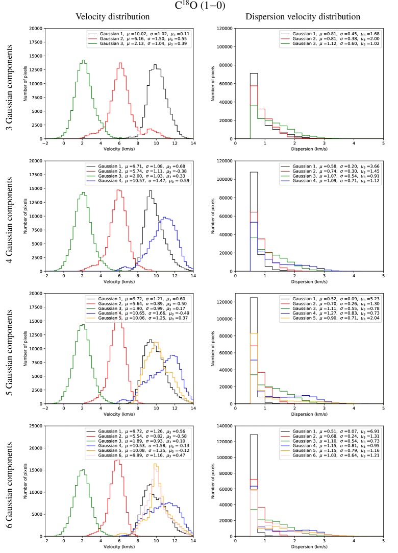
Figure 12: Distributions in velocity (left) and velocity dispersion (right) of each Gaussian component from the different decompositions using different numbers $N$ of Gaussian components. The mean, variance and skewness of each distribution are shown in legend.

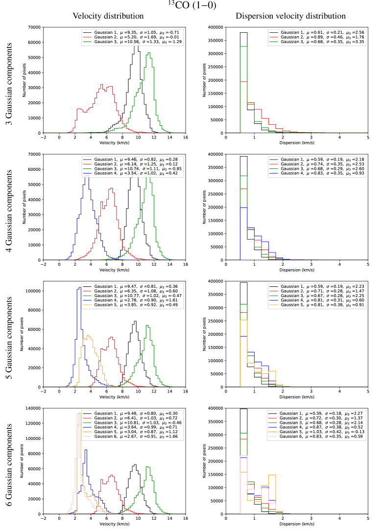
Figure 13: Distributions in velocity (left) and velocity dispersion (right) of each Gaussian component from the different decompositions using different numbers $N$ of Gaussian components. The mean, variance and skewness of each distribution are shown in legend.

A.2 Best hyper-parameters

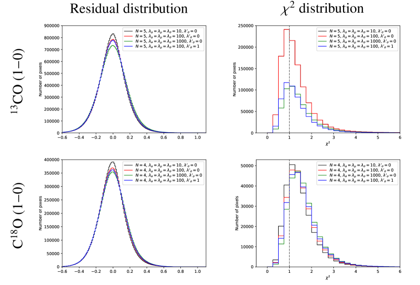
Figure 14: Residual (left) and $\chi^{2}$ (right) distributions between the original and the ROHSA reconstructed cubes for a given number of Gaussian components (four for C¹⁸O and five for ¹³CO) and different hyper-parameters $\lambda_{\mathrm{i}}$ from the ¹³CO (1$-$0) (top) and C¹⁸O (1$-$0) (bottom) emission, respectively.

To find the best hyper-parameters, we also set up the algorithm with several values ($\lambda_{\mathrm{i}}$= [10, 100, 1000], $\lambda^{\prime}_{\mathrm{\sigma}}$= [0, 1]) for the best total number of Gaussian components $N_{\mathrm{best}}$. After building the associated $\chi^{2}$ and residual distributions, we observe that the Gaussian decompositions do not show distributions very different from each other to identify robustly the best hyper-parameters (see Fig. 14). We selected $\lambda_{\mathrm{i}}$=100 for each hyper-parameter. The hyper-parameter $\lambda^{\prime}_{\mathrm{\sigma}}$ have been set to $0$ to let free the variation of the velocity dispersion across the map throughout the full field of view.

Appendix B Moment maps of the Gaussian components for each tracer

Appendix C Monte Carlo simulations

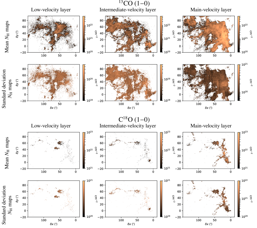
Figure 18: Mean and standard deviation on the $N_{\mathrm{H}}$ values from ¹³CO (1$-$0) (top) and C¹⁸O (1$-$0) (bottom) implemented during the Monte-Carlo process for the three layers of the Orion B cloud, namely the low-velocity layer (left), the intermediate-velocity layer (middle), and the main-velocity layer (right) rebuilt by ROHSA. Isolated pixels and pixels with a signal-to-noise ratio lower than 3 are blanked.

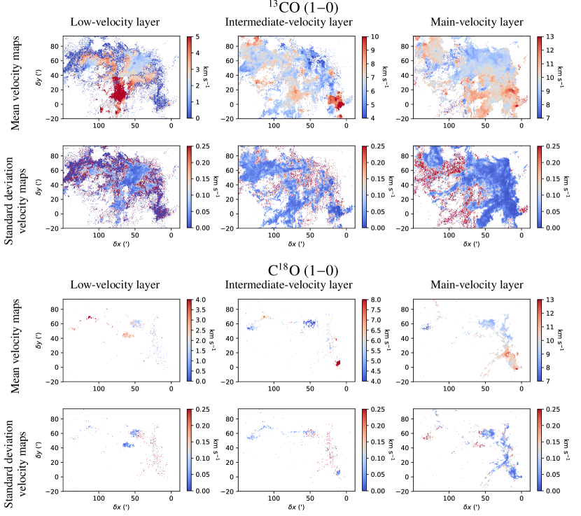
Figure 19: Mean and standard deviation on the centroid velocity values from ¹³CO (1$-$0) (top) and C¹⁸O (1$-$0) (bottom) implemented during the Monte-Carlo process for the three layers of the Orion B cloud, namely the low-velocity layer (left), the intermediate-velocity layer (middle), and the main-velocity layer (right) rebuilt by ROHSA. Isolated pixels and pixels with a signal-to-noise ratio lower than 3 are blanked.

Appendix D Comments on individual subregions

This section shows the detailed results for all subregions sorted from east to west, and then from north to south.

D.1 Intermediate-velocity layer, Cloak

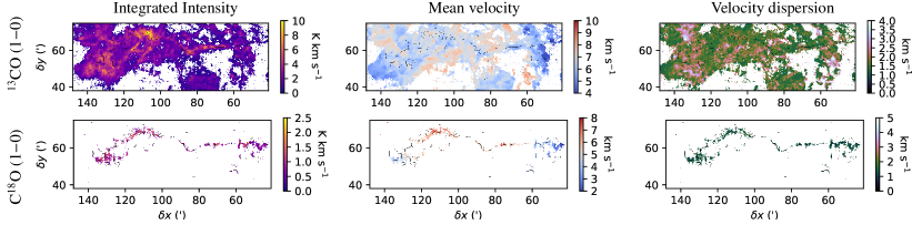
Figure 20: Zero-order (integrated intensity, left), first-order (mean velocity, middle), and second-order (velocity dispersion, right) moment maps in the Cloak area from the intermediate-velocity layer, from the ¹³CO (1$-$0) (top) and C¹⁸O (1$-$0) (bottom) emission reconstructed by ROHSA. The black lines show the filamentary structures extracted from C¹⁸O (1$-$0).

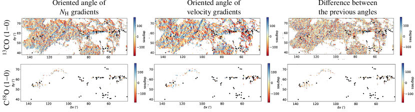
Figure 21: Maps of the column density gradient oriented angles (top) and the velocity gradient oriented angles (middle) in the Cloak area from the intermediate-velocity from the ¹³CO (1$-$0) (left) and the C¹⁸O (1$-$0) (right) emission. Bottom: maps of the relative orientation between the oriented angles of the column density and the velocity gradients. Oriented angles are defined north from east. The black lines show the filamentary structure and the diamond dots show the dense cores.

Figure 22: Divergence maps of the column density gradients in N_H pix^-1 (left) and the velocity gradients in km s^-1 pix^-1 (middle) for the intermediate-velocity layer of the Cloak area from the ¹³CO (1$-$0) (top) and the C¹⁸O (1$-$0) (bottom) emission. Right: comparison maps of the sign between the velocity gradient divergence and the column density gradient divergence. The values -1 (blue) or 1 (red) show the pixels where velocity and column density gradients both converge or both diverge. The value 0 (gray) indicates regions where the sign of at least one gradient is ill-defined because its modulus is close to zero. The black lines show the filamentary structure and the diamond dots show the dense cores identified by the Herschel Gould Belt Survey (Könyves et al. 2020).

According to Greek mythology, the constellation of Orion represents a hunter. The CO emission from the main-velocity layer looks like a human skeleton with the head at the Hummingbird filament and the two feet at the Flame filament and the Horsehead Nebula (see Fig. 2). The Cloak area was named as such because the CO emission from this layer is filamentary and located to the northeast of the NGC 2023 and NGC 2024 star-forming regions, like a knight’s cloak.

The HGBS mapped this area and reveals that it is actually composed of a long filamentary structure that follows the Cloak shape from east to west in which several starless and pre-stellar cores appear to be embedded (Könyves et al. 2020). This is quite consistent with the filamentary network we extracted from the C¹⁸O emission of the intermediate-velocity layer. However, we identified a network of small filaments that follow the Cloak shape from east to west instead of a long single filament. This is due to the structure of the C¹⁸O emission, which is faint and not continuous (see Fig. 20).

There are very few or no studies of the kinematics of this region. The velocity map from the C¹⁸O emission (see Fig. 20) shows an oscillation in blue- and red-shifted velocities along the entire filamentary structure. Other filaments, as G350.5-N filament (Liu et al. 2019), exhibit this kind of velocity pattern. It may suggest either an oscillation of the filament toward and away from the observer or motions due to core formation along the filamentary structure. However, at larger scales, from the ¹³CO emission, the velocity patterns are more complex than an oscillation along the filamentary network.

D.2 Low- and intermediate-velocity layer, Orion B9

Orion B9 is an active star-forming region of the Orion B molecular cloud. Miettinen et al. (2009) mapped the Orion B9 region at 870 $\mu$m and identified 12 dense cores. Six of them are associated with Spitzer 24 $\mu$m sources, and are therefore identified as protostellar objects. The remaining cores have no mid-infrared counterparts but are gravitationally bound (Miettinen et al. 2010), and thus they can be considered as pre-stellar cores. The HGBS images revealed that Orion B9 is actually composed of supercritical filaments in which pre- and protostellar cores appear to be embedded (Könyves et al. 2020). However, the HGBS data set does not distinguish the different components in velocity we identified.

From multiple line observations, Miettinen (2012, 2020) find two separated velocity components at about 1.5$-$5 and 8.5$-$9.5 km s^-1 in several protostellar objects. These velocity components are consistent with the low-velocity layer at 0$-$4 km s^-1 and the main-velocity layer at 8$-$10.5 km s^-1 we identified in this study from both ¹³CO and C¹⁸O (1$-$0) observations (see Figs. 23 and 26). Miettinen (2012) detect a velocity gradient along the northwestern-southeastern direction in the two different velocity components from C¹⁸O (2$-$1) observations. The direction of this gradient is consistent with the one we observe in the Orion B9 area from ¹³CO and C¹⁸O (1$-$0) observations, from both the low-velocity and the main-velocity layers (see Figs. 23 and 26). Miettinen (2012, 2020) interpret this gradient as due to a collision between two clouds. The collision may be triggered by the expansion of the H ii region of NGC 2024 that lies about 4 pc to the southwest of Orion B9 region. This collision would be responsible for filament and dense core formation in Orion B9 area.

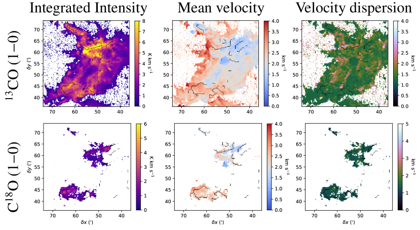
Figure 23: Moment maps for the low-velocity layer of the Orion B9 area. The figure layout is identical to Fig. 20.

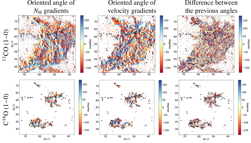
Figure 24: Maps of oriented angles of the gradients of the column density and centroid velocity gradients for the low-velocity layer of the Orion B9 area. The figure layout is identical to Fig. 21

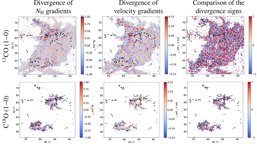
Figure 25: Divergence maps for the low-velocity layer of the Orion B9 area. The figure layout is identical to Fig. 21

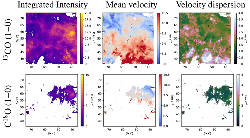
Figure 26: Moment maps for the main-velocity layer of the Orion B9 area. The figure layout is identical to Fig. 20.

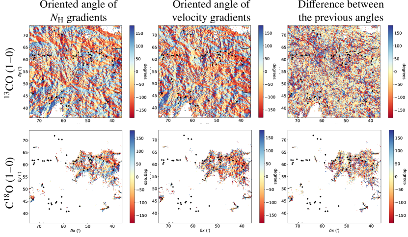
Figure 27: Maps of oriented angles of the gradients of the column density and centroid velocity gradients for the main-velocity layer of the Orion B9 area. The figure layout is identical to Fig. 21

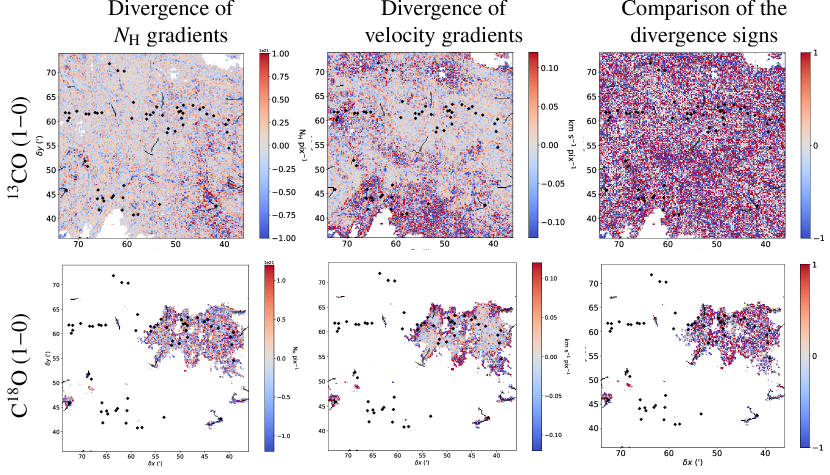
Figure 28: Divergence maps for the main-velocity layer of the Orion B9 area. The figure layout is identical to Fig. 21

D.3 Main-velocity layer, Hummingbird filament

The velocity map from the C¹⁸O emission (see Fig. 29) shows an oscillation in blue- and red-shifted velocities along the main filamentary structure. Other filaments, as G350.5-N filament (Liu et al. 2019) and the Cloak filament (see Fig. 20), exhibit this kind of velocity pattern. It may suggest either an oscillation of the filament toward and away from the observer or motions due to core formation along the filamentary structure. Orkisz et al. (2019) also identify hints of periodic longitudinal fragmentation along the Hummingbird filament. However, they estimated that this filament is gravitationally subcritical and very few known YSOs are embedded in it. Thus, this velocity oscillation is unlikely to be due to core formation.

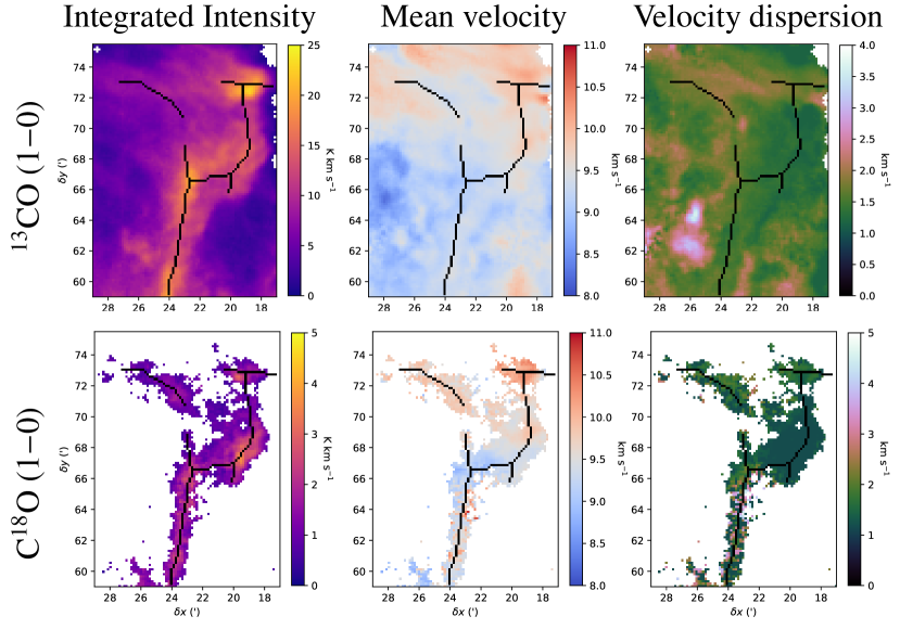
Figure 29: Moment maps for the main-velocity layer of the Hummingbird area. The figure layout is identical to Fig. 20.

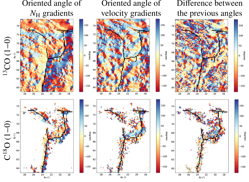
Figure 30: Maps of oriented angles of the gradients of the column density and centroid velocity gradients for the main-velocity layer of the Hummingbird area. The figure layout is identical to Fig. 21

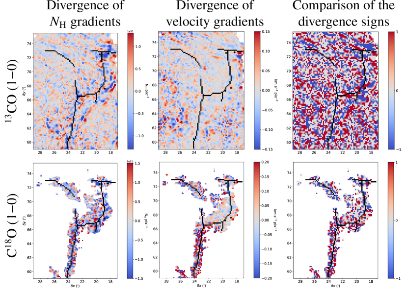
Figure 31: Divergence maps for the main-velocity layer of the Hummingbird area. The figure layout is identical to Fig. 21

D.4 Main-velocity layer, intermediate area

The Intermediate area was named this way because it is located between two well-studied areas: NGC 2024 and the Hummingbird filament. There are very few or no studies of the kinematics of this region but its kinematics is interesting to study because it encompasses the northern edge of the NGC 2024 H ii region.

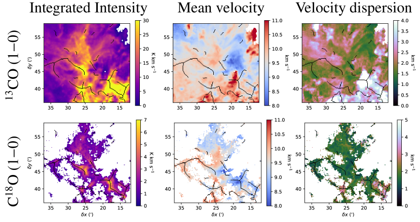
Figure 32: Moment maps for the main-velocity layer of the Intermediate area. The figure layout is identical to Fig. 20.

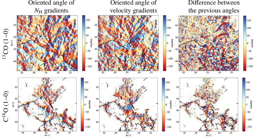
Figure 33: Maps of oriented angles of the gradients of the column density and centroid velocity gradients for the main-velocity layer of the Intermediate area. The figure layout is identical to Fig. 21

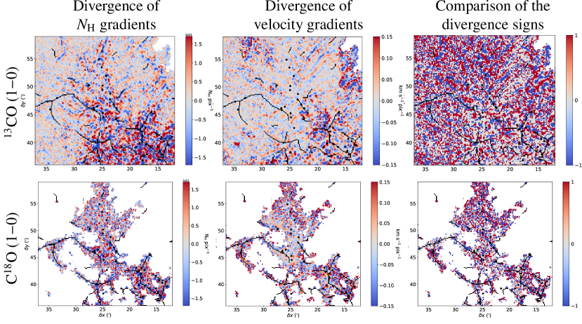
Figure 34: Divergence maps for the main-velocity layer of the Intermediate area. The figure layout is identical to Fig. 21

D.5 Main-velocity layer, NGC 2024

NGC 2024, also known as the Flame Nebula, is a well-known massive star-forming region. From ¹²CO and ¹³CO observations, Emprechtinger et al. (2009) found that most of this region consists of a hot (75 K) and dense (9 $\times$ 10⁵ cm^-2) gas. From ¹³CO (2$-$1) observations, Enokiya et al. (2021) find two velocity components with a velocity separation of $\sim$2 km s^-1 (8.5$-$9.5 km s^-1 and 10.5$-$11.5 km s^-1) in the region including NGC 2023, NGC 2024 and the Horsehead Nebula. Both components are associated with the main-velocity layer. This suggests that a major cloud-cloud collision, with a timescale of 2 $\times$ 10⁵ yr, triggered the formation of massive stars in NGC 2024, including the late O or early B massive star IRS2b. IRS2b has been identified as the main ionizing source of NGC 2024 (Bik et al. 2003). The associated H ii region is expected to expand into the molecular cloud and to trigger star formation.

Maps of dust emission at 1 mm by Mezger et al. (1988, 1992) exhibit high-density condensations aligned in an elongated ridge running north to south, consistent with the filamentary structure we identified at the center of the region (see Fig. 35). Submillimeter and millimeter observations revealed outflows associated with some of the dense condensations, which would therefore be young protostars (Moore & Yamashita 1995; Richer et al. 1992; Richer 1990). Choi et al. (2012) also detected H₂O and CH₃OH maser lines in NGC 2024, suggesting that this region is actively forming stars.

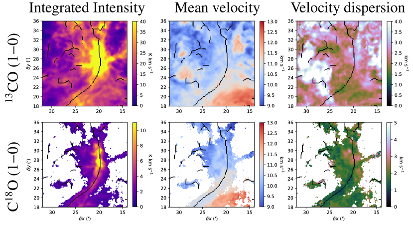
Figure 35: Moment maps for the main-velocity layer of the NGC 2024 area. The figure layout is identical to Fig. 20.

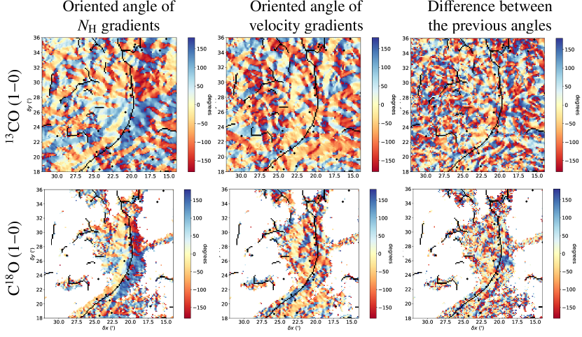
Figure 36: Maps of oriented angles of the gradients of the column density and centroid velocity gradients for the main-velocity layer of the NGC 2024 area. The figure layout is identical to Fig. 21

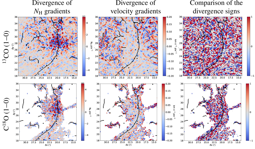
Figure 37: Divergence maps for the main-velocity layer of the NGC 2024 area. The figure layout is identical to Fig. 21

D.6 Main-velocity layer, Flame filament

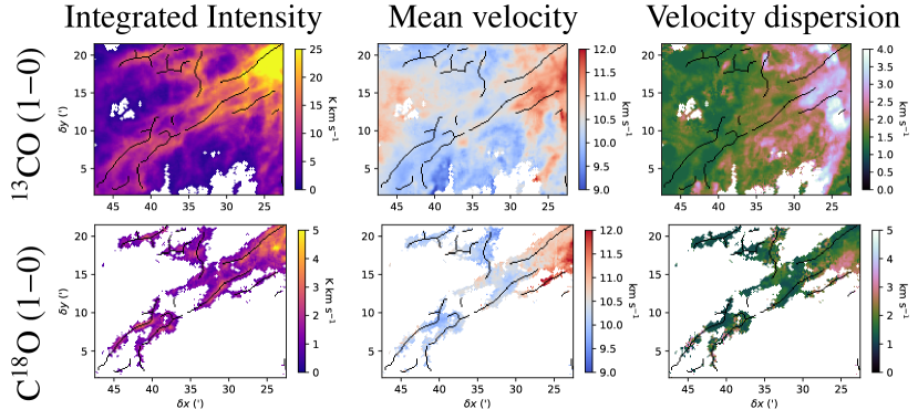
Figure 38: Moment maps for the main-velocity layer of the Flame Filament area. The figure layout is identical to Fig. 20.

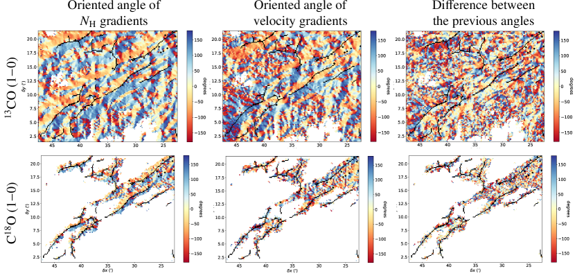
Figure 39: Maps of oriented angles of the gradients of the column density and centroid velocity gradients for the main-velocity layer of the Flame Filament area. The figure layout is identical to Fig. 21

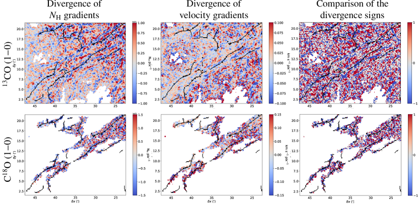
Figure 40: Divergence maps for the main-velocity layer of the Flame Filament area. The figure layout is identical to Fig. 21

D.7 Main-velocity layer, Horsehead Nebula

The Horsehead Nebula, also known as Barnard 33, is one of the most easily recognizable shape in the sky. At visible wavelengths, it appears as a 5-arcminute dark patch against the bright H$\alpha$ emission. Philipp et al. (2006) determined that the UV radiation primarily comes from $\sigma$Ori. High density gas and UV stellar light interact at the edge of the western condensation, forming a photon-dominated region. At 400pc, the Horsehead Nebula is the closest known pillar (Pound et al. 2003). Reipurth & Bouchet (1984) suggested that the Horsehead Nebula formed through the photo-evaporation of low density material around the neck, shaping the molecular cloud into the famous Horsehead. Hily-Blant et al. (2005) measured velocity gradients from the C¹⁸O (2$-$1) emission and suggested that the gas is rotating around the neck axis with a rotation period of $\sim$4 Myr. They also found two dense condensations that were identified as dense cores by Ward-Thompson et al. (2006). The Horsehead Nebula is an active star-forming region since Bowler et al. (2009) found also five candidate young stars, a class II YSO, and two protostars.

While the majority of the emission of the Horsehead Nebula is associated with the main-velocity layer, we can see that a spatial component corresponds to NGC 2023 and the Horsehead Nebula in the C¹⁸O and ¹³CO (1$-$0) emissions of the Cloak layer (see Fig. 4). Thus, NGC 2023 and the Horsehead Nebula have two velocity components, a first one at 6$-$9.5 km s^-1 (associated with the intermediate-velocity layer) and a main one at 10$-$12 km s^-1 (associated with the main-velocity layer).

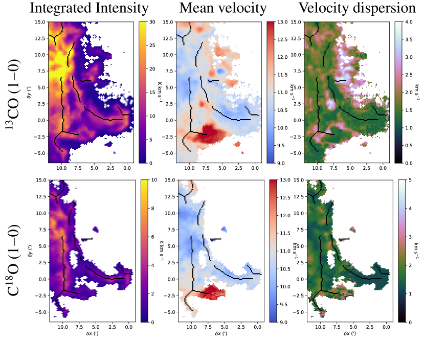
Figure 41: Moment maps for the main-velocity layer of the Horsehead Nebula area. The figure layout is identical to Fig. 20.

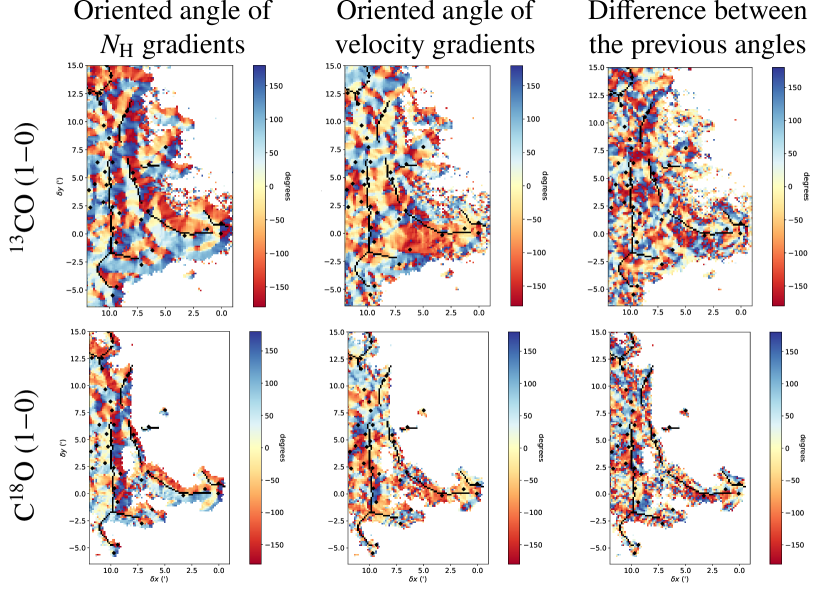
Figure 42: Maps of oriented angles of the gradients of the column density and centroid velocity gradients for the main-velocity layer of the Horsehead Nebula area. The figure layout is identical to Fig. 21

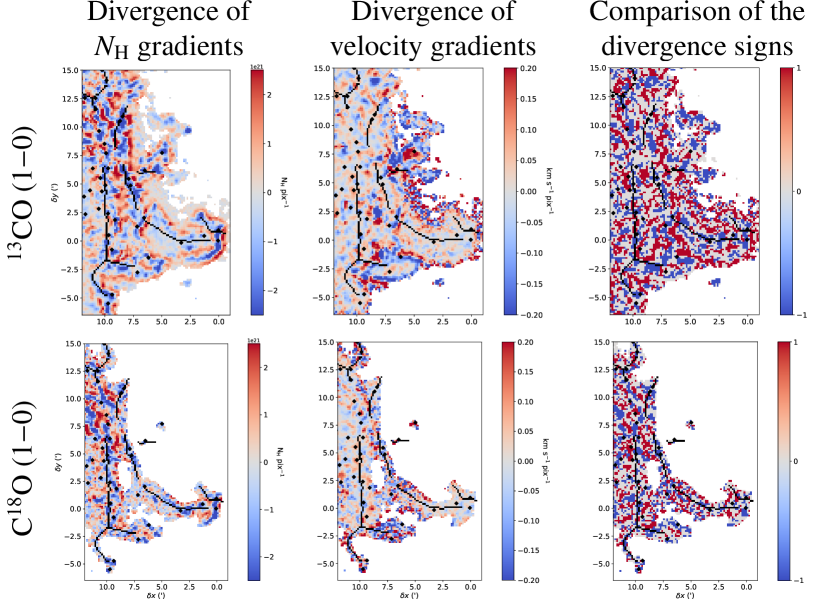
Figure 43: Divergence maps for the main-velocity layer of the Horsehead Nebula area. The figure layout is identical to Fig. 21

Appendix E Influence of the Gaussian decomposition on the kinematic results

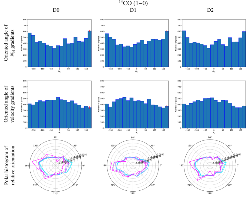
Figure 44: ¹³CO distribution histogram of the oriented angles of the column density (top row) and velocity gradients (middle row) in the Horsehead nebula from the reference decomposition $\mathrm{D0}$ (left), decomposition $\mathrm{D1}$ (middle) and decomposition $\mathrm{D2}$ (right), respectively. Last row: histograms of the relative orientation between column density and velocity. Data with $\log(N_{\mathrm{H}}^{13})>20.00$ cm^-2 are shown in cyan, $\log(N_{\mathrm{H}}^{13})>21.00$ cm^-2 in blue, $\log(N_{\mathrm{H}}^{13})>21.55$ cm^-2 in blue-violet, $\log(N_{\mathrm{H}}^{13})>22.00$ cm^-2 in purple, and $\log(N_{\mathrm{H}}^{13})>22.40$ cm^-2 in fuchsia. The colored bars at 10^∘ show the error bars of the histograms.

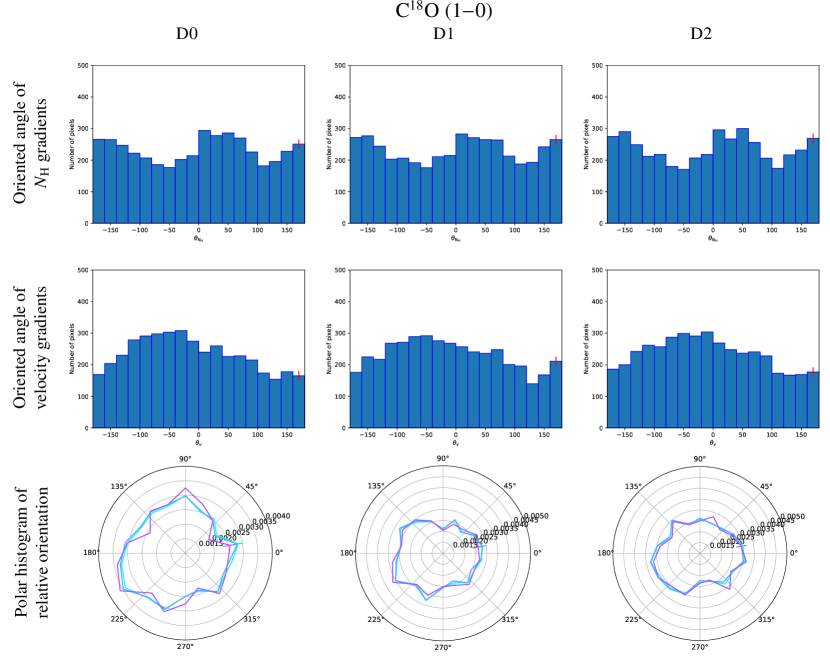
Figure 45: C¹⁸O distribution histogram of the oriented angles of the column density (top row) and velocity gradients (middle row) in the Horsehead nebula from the reference decomposition $\mathrm{D0}$ (left), decomposition $\mathrm{D1}$ (middle) and decomposition $\mathrm{D2}$ (right), respectively. Last row: histograms of the relative orientation between column density and velocity. Data with $\log(N_{\mathrm{H}}^{18})>21.00$ cm^-2 are shown in cyan, $\log(N_{\mathrm{H}}^{18})>21.55$ cm^-2 in blue-violet, $\log(N_{\mathrm{H}}^{18})>22.00$ cm^-2 in purple, and $\log(N_{\mathrm{H}}^{18})>22.40$ cm^-2 in fuchsia. The colored bars at 10^∘ show the error bars of the histograms.

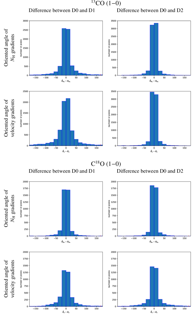
Figure 46: Difference between the oriented angles of the gradients obtained in the Horsehead nebula from $\mathrm{D0}$ and from $\mathrm{D1}$ (left), and from $\mathrm{D0}$ and from $\mathrm{D2}$ (right), respectively.

To characterize the influence of the choice of hyper-parameters of the ROHSA Gaussian decomposition on the moment maps and, thus, on velocity and column density gradients, we set up the algorithm to decompose the ¹³CO and C¹⁸O signals with different hyper-parameters for the best total number of Gaussian components determined above. As example, we chose the two following sets of hyper-parameters: ($\lambda_{\mathrm{A}}=\lambda_{\mathrm{\mu}}=\lambda_{\mathrm{\sigma}}=10$, $\lambda^{\prime}_{\mathrm{\sigma}}=0$) and ($\lambda_{\mathrm{A}}=\lambda_{\mathrm{\mu}}=\lambda_{\mathrm{\sigma}}=100$, $\lambda^{\prime}_{\mathrm{\sigma}}=1$). In the following, these two decompositions are denoted as $\mathrm{D1}$ and $\mathrm{D2}$. $\mathrm{D1}$ forces the spatial coherence of the Gaussian components in the field of view a little less than the decomposition chosen and presented in the main text, namely the decomposition $\mathrm{D0}$ with the set of hyper-parameters: $\lambda_{\mathrm{A}}=\lambda_{\mathrm{\mu}}=\lambda_{\mathrm{\sigma}}=100$, $\lambda^{\prime}_{\mathrm{\sigma}}=0$. $\mathrm{D2}$ puts a constrain on the $\sigma$ variation of Gaussian components along the field of view compared to $\mathrm{D0}$.

From these decompositions, we followed the same methodology as described above, namely, the construction of moment maps to identify the different layers in the Orion B cloud and the computation of the errors on the velocity and the column density via a Monte Carlo process to select only the robust pixels (i.e., $N_{\mathrm{H}}>10^{20}$ cm^-2 for ¹³CO, $N_{\mathrm{H}}>10^{21}$ cm^-2 for C¹⁸O, and error on the velocity $<$0.25 km s^-1).

In the following, we present the kinematic results obtained from $\mathrm{D1}$ and $\mathrm{D2}$ for the ¹³CO and C¹⁸O emission of the Horsehead Nebula and we compare them with the $\mathrm{D0}$ results showed in the main text. Figures 44 and 45 show the distribution histogram of the oriented angles of the column density and velocity gradient in the Horsehead Nebula and the histograms of the relative orientation between both gradients to compare the results from the different decompositions. The trend of the histograms is the same and the small visible variations between the different decompositions are consistent with the error bars of the histograms. Figure 46 shows the variation of the column density and velocity gradient orientation in the Horsehead Nebula from D1 and D2 decompositions with respect to D0 one. There is very little variation in the orientation of the gradients. For velocity gradients, the variation in orientation is mostly between -20^∘ and 20^∘, which is consistent with the error distribution estimated from the Monte Carlo process.

Appendix F Simple 3D model of a filament and its associated velocity field

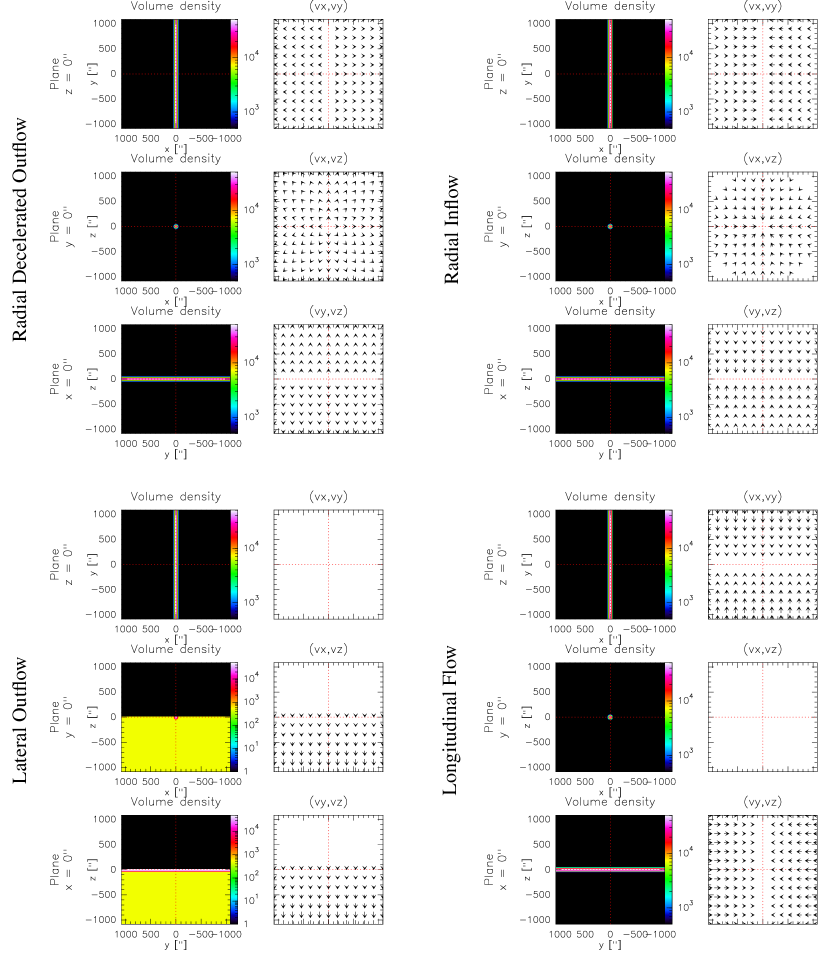
Figure 47: 2D cuts along different plane of the 3D density (left) and velocity (right) fields for the four different models. The radial decelerated outflow is shown in the top left corner, the radial inflow in the top right corner, the lateral outflow in the bottom left corner and the longitudinal flow in the bottom right corner.

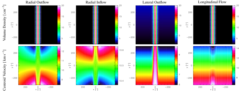
Figure 48: Spatial distribution of the projected column density (top) and centroid velocity (bottom) for the different models. The gradient vectors are overlaid.

F.1 Volume density

F.1.1 Typical case

In a 3D cube of dimensions $241\times 241\times 241$ pixels with a central position at the coordinates $(\mu_{x},\mu_{y},\mu_{z})=(121,121,121),$ we modeled a simple isolated filament using an infinite cylinder along the $y$-axis, whose section in the $xz$ plane follows a 2D Gaussian function. We used $n_{\mathrm{H_{0}}}$ as an amplitude factor for the density, and $\sigma_{x}=\sigma_{z}=\sigma_{xz}$ the standard deviation of the density distribution along the $x$- and $z$-axes. We define the radius perpendicular to the filament as $r=\sqrt{(x-\mu_{x})^{2}+(z-\mu_{z})^{2}}$. With these definitions, the density distribution of the filament $n_{\mathrm{fil}}$ is

$$n_{\mathrm{fil}}(x,y,z)=n_{\mathrm{H_{0}}}\exp{\left\{-\frac{r^{2}}{2\sigma_{xz}^{2}}\right\}}.$$ (4)

We modeled the filament at the central position of the 3D cube with a Gaussian full width at half maximum of 4 pixels for the $x$- and $z$-axes. The pixel size is $9^{\prime\prime}$ or $17.5\mathrm{\,mpc}$ at a distance of 400 pc. The filament is immersed in a constant density background $n_{\mathrm{bg}}$. The total density of the cube is therefore represented by $n_{\mathrm{tot}}(x,y,z)=n_{\mathrm{fil}}(x,y,z)+n_{\mathrm{bg}}(x,y,z)$ with $n_{\mathrm{H_{0}}}=5\times 10^{4}\mathrm{\,cm^{-3}}$, and $n_{\mathrm{bg}}(x,y,z)=5\times 10^{2}\mathrm{\,cm^{-3}}$. Figure 47 shows the three 2D cuts of the volume density.

F.1.2 Ionized-like case

Some of the filaments in the ORION-B field of view are localized at the interface between the molecular cloud and an H ii region. We thus developed a model where only the molecular half of the space emits. To do this, we kept the same typical volume density field, except that we set the volume density to zero for half of the cube along the $z$-axis.

F.2 Velocity field

We developed four models of velocity fields representative of the different physical processes: 1) a radial inflow corresponding to accretion onto the filament, 2) a radial decelerated outflow in case the filament would host a star, 3) a lateral flow from the filament to the diffuse environment representing a filament at the edge of an H ii region, and 4) a longitudinal flow along the filament axis. Figure 47 shows the associated velocity vectors in three 2D planes.

F.2.1 Radial inflow and outflow

For the radial flows, we introduced $\beta(x,z)$, the velocity angle in the $(x,z)$ plane so that

$$\cos\beta(x,z)=\frac{x-\mu_{x}}{r},\quad\mbox{and}\quad\sin\beta(x,z)=\frac{z-\mu_{z}}{r},$$ (5)

where $\mu_{x}$ and $\mu_{z}$ are the positions of the center of the filament. The components of the radial velocity gradient are then defined as

$$V_{x}(x,y,z) = V(r)\,\cos{\beta(x,z)},$$ (6)

$$V_{y}(x,y,z) = 0,$$ (7)

$$V_{z}(x,y,z) = V(r)\,\sin{\beta(x,z)},$$ (8)

where $V(r)$ is the amplitude of the velocity field at the distance $r$ from the filament center. We considered two possibilities for the velocity amplitude, namely,

a decelerated outflow,

$$V(r)=\frac{50\mathrm{\,km\,s^{-1}}}{\sqrt{1+\left(\frac{r}{r_{0}}\right)^{2}}\,\left[1+\frac{n_{\mathrm{H_{0}}}}{n_{\mathrm{bg}}}\exp\left\{-\left(\frac{r}{r_{0}}\right)^{2}\right\}\right]};$$ (9)

and a gravitational inflow,

$$V(r)=-2\sqrt{G\,m_{\mathrm{lin}}(r)\,\log\left(\frac{r_{\mathrm{max}}}{r}\right)},$$ (10)

where $m_{\mathrm{lin}}$ is the linear mass inside the cylinder of radius $r$, given by

$$m_{\mathrm{lin}}(r)=\pi\,\mu\,n_{\mathrm{H_{0}}}\,r_{0}^{2}\left[1-\exp\left(-\frac{r^{2}}{r_{0}^{2}}\right)\right].$$ (11)

This follows the models by Heitsch (2013a, b). It can be rewritten as

$$V(r)=-V_{0}\sqrt{\left[1-\exp\left(-\frac{r^{2}}{r_{0}^{2}}\right)\right]\,\log\left(\frac{r_{\mathrm{max}}}{r}\right)}$$ (12)

$$\mbox{with}\quad V_{0}=2\sqrt{\pi\,G\,\mu\,n_{\mathrm{H_{0}}}\,r_{0}^{2}}\sim 0.23\mathrm{\,km\,s^{-1}}.$$ (13)

For these two possibilities, $r_{0}$ is a scaling parameter that defines the scale of the gradient. We chose the same value as the full width at half maximum of the filament, 4 pixels. For the gravitational inflow, $r_{\mathrm{max}}$ is the starting point of the inflow and $\mu$ is the mean molecular mass of the gas (i.e., $\mu\simeq 2.5m_{\mathrm{H}}$). We chose $r_{\mathrm{max}}=L/2$ with $L$ the length of the cube.

F.2.2 Lateral flow

The gas is accelerating from one side to another side of the 3D cube through the filament. This simple scenario could be expected by the expansion of a H ii region pushing matter outward, the other part of the gas being ionized, or to a lateral pressure exerted on the high density filament from a lower density expanding structure, a bubble of hot gas for instance. In this model, the gas is decelerating from the outside region to the filament.

F.2.3 Longitudinal flow

In this case, the flow is parallel to the filament axis (i.e., along the $y$ direction) and converges toward the plane $y=0^{\prime\prime}$:

$$V_{x}(x,y,z) = 0,$$ (14)

$$V_{y}(x,y,z) = -V_{0}\,y,$$ (15)

$$V_{z}(x,y,z) = 0,$$ (16)

where $V_{0}$ is a constant that we set to $0.5\mathrm{\,km\,s^{-1}}$. This case belongs to the family of scenarios where the gas flow converges parallel to the filament to form a dense core.

F.3 Projection onto the plane of the sky

The models are computed in three dimensions in a coordinate frame that is adapted to the geometry of the filament. However, the filament is probably inclined on the plane of the sky and the observer will only have access to values projected onto the plane of the sky. In order to deal with the inclination on the plane of the sky, we rotated the position and velocity vectors around an axis parallel to the $x$-axis and we then interpolated the values of the density and velocity coordinates into the inclined coordinate system with new axes $(x^{\prime},y^{\prime},z^{\prime})$. This generates edge effects because the initial cubes has a limited size. To avoid these “artifacts,” we extracted an inner cube of $69^{3}$ pixels. The column density was then computed by integrating the volume density along the line of sight with

$$N(x^{\prime},y^{\prime})=\frac{L}{N_{\mathrm{pix}}}\sum_{z^{\prime}}n_{\mathrm{tot}}(x^{\prime},y^{\prime},z^{\prime}).$$ (17)

We computed the centroid velocity and its gradient in the optically thin limit,

$$C_{V}(x^{\prime},y^{\prime})=\frac{\sum_{z^{\prime}}n_{\mathrm{tot}}(x^{\prime},y^{\prime},z^{\prime})V_{z^{\prime}}(x^{\prime},y^{\prime},z^{\prime})}{\sum_{z^{\prime}}n_{\mathrm{tot}}(x^{\prime},y^{\prime},z^{\prime})}.$$ (18)

All models were computed for different inclinations of the filament along the line of sight to investigate the effect of inclination and we selected the models for a typical inclination of $30^{\circ}$. Figure 48 shows the resulting maps of column density and centroid velocity. The vectors of their gradient are overlaid. All the models shown in this appendix are inclined on the plane of sky around an axis located in the middle of the field of view but we discuss in the main text the effect of varying the position of the inclination axis.