WALDO: Future Video Synthesis using Object Layer Decomposition and Parametric Flow Prediction

Abstract

This paper presents WALDO (WArping Layer-Decomposed Objects), a novel approach to the prediction of future video frames from past ones. Individual images are decomposed into multiple layers combining object masks and a small set of control points. The layer structure is shared across all frames in each video to build dense inter-frame connections. Complex scene motions are modeled by combining parametric geometric transformations associated with individual layers, and video synthesis is broken down into discovering the layers associated with past frames, predicting the corresponding transformations for upcoming ones and warping the associated object regions accordingly, and filling in the remaining image parts. Extensive experiments on multiple benchmarks including urban videos (Cityscapes and KITTI) and videos featuring nonrigid motions (UCF-Sports and H3.6M), show that our method consistently outperforms the state of the art by a significant margin in every case. Code, pretrained models, and video samples synthesized by our approach can be found in the project webpage.

1 Introduction

Predicting the future from a video stream is an important tool to make autonomous agents more robust and safe. In this paper, we are interested in the case where future frames are synthesized from a fixed number of past ones. One possibility is to build on advanced image synthesis models [59, 23, 44, 20] and adapt them to predict new frames conditioned on past ones [79]. Extending these already memory- and compute-intensive methods to our task may, however, lead to prohibitive costs due to the extra temporal dimension. Hence, the resolution of videos predicted by this approach is often limited [95, 36, 96]. Other works resort to compression [82, 64] to reduce computations [103, 97, 63], at the potential cost of poorer temporal consistency [61].

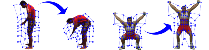
$T$

$T{+}10$

$T$

$T{+}10$

Figure 1: WALDO synthesizes future frames by deforming grids of control points, automatically associated with different objects.

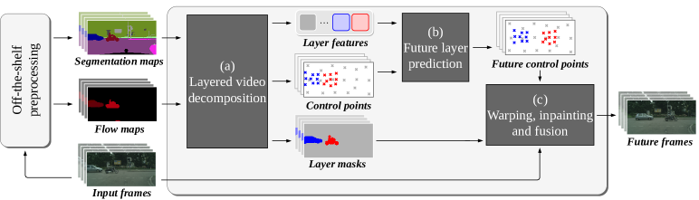
Figure 2: Overview of WALDO. Given an input video sequence and associated semantic segmentation and optical flow maps preprocessed by off-the-shelf models [77, 14], our approach breaks down video synthesis into (a) layered video decomposition: using semantic and motion cues to decompose the sequence into layers represented by both object masks and features, with spatial information in the form of a small set of control points, (b) future layer prediction: predicting the new position of these points in the target output frames, and (c) warping, inpainting and fusion: using the corresponding offset and a thin-plate spline deformation model to warp the input frames and object masks, merge the corresponding regions, and fill in the empty image parts. Our model is trained, without explicit annotations, on a set of videos of $T{+}K$ frames by using the first $T$ to predict the next $K$. At inference, a (potentially greater) number $K$ of frames is predicted from $T$ input ones by repeating (a), (b) and (c) in an autoregressive fashion if needed.

Our work relies instead on semantic and motion cues extracted from the past to model complex dynamics in high resolution and predict the future. Wu et al. [99] decompose scenes into objects/background, predict affine transformations for the objects and non-affine ones for the background, and warp the last input frame to produce new ones. Bei et al. [7] predict dense flow maps for individual semantic regions. Geng et al. [29] augment classical frame reconstruction losses with flow-based correspondences between pairs of frames. Wu et al. [100] build on a pretrained video frame interpolation model which they adapt to future video prediction. Contrary to [99], our model automatically discovers the object decomposition without explicit supervision. Moreover, rather than directly predicting optical flow at each pixel [99, 7, 100], we use thin-plate splines (TPS) [9] as a parametric model of per layer flow for any pair of frames. This improves robustness since we predict future frames using all past ones as opposed to [99, 7, 29, 100]. In addition, TPS provide optical flow at any resolution, and allow using a lower resolution for fast training while retaining good performance with high-resolution inputs at inference. Lastly, a few time-dependent control points associated with each object and the background are sufficient to parameterize TPS. This compact yet expressive representation of motion allows us to break down video synthesis into: (a) discovering the layers associated with past frames, (b) predicting the corresponding transformations for upcoming ones while handling complex motions [13] and modeling future uncertainty if needed [1, 2], and (c) warping the associated object regions accordingly and filling in the remaining image parts. By combining these three components, our approach (Figure 2) to predict future frames by WArping Layer-Decomposed Objects (WALDO) from past ones sets a new state of the art on diverse benchmarks including urban scenes (Cityscapes [17] and KITTI [28]), and scenes featuring nonrigid motions (UCF-Sports [67] and H3.6M [41]). Our main contributions are twofold:

$\bullet$ Much broader operating assumptions: Previous approaches to video prediction that decompose individual frames into layers assume prior foreground/background knowledge [99] or reliable keypoint detection [88, 106], and they do not allow the recovery of dense scene flow at arbitrary resolutions for arbitrary pairs of frames [99, 7, 29, 100, 1, 2, 13]. Our approach overcomes these limitations. Unlike [99, 7, 29, 100, 13], it also allows multiple predictions.

$\bullet$ Novelty: The main novelties of our approach to video prediction are (a) a layer decomposition algorithm that leverages a transformer architecture to exploit long-range dependencies between semantic and motion cues; (b) a low-parameter deformation model that allows the long-term prediction of sharp frames from a small set of adjustable control points; and (c) the effective fusion of multiple predictions from past frames using state-of-the-art inpainting to handle (dis)occlusion. Some of these elements have been used separately in the past (e.g., [104, 106, 61]), but never, to the best of our knowledge, in an integrated setting.

These contributions are validated through extensive experiments on urban datasets (Cityscapes and KITTI), as well as scenes featuring nonrigid motions (UCF-Sports, H3.6M), where our method outperforms the state of the art by a significant margin in every case

2 Related work

Video prediction

ranges from unconditional synthesis [80, 19, 86, 25, 16, 69, 79, 24, 4, 47] to multi-modal and controlled prediction tasks [33, 61, 97, 32, 38]. Here, we intend to exploit the temporal redundancy of videos by tracking the trajectories of different objects. One may infer future frames by extrapolating the position of keypoints associated to target objects [88, 106], but this requires manual labeling. Some works [12, 37, 60, 34, 21] propose instead to let structured object-related information naturally emerge from the videos themselves. We use a similar strategy but also rely on off-the-shelf models to extract semantic and motion cues in the hope of better capturing the scene dynamics [90, 7, 71, 99, 29, 100]. Without access to ground-truth objects, we discover them via layered video decomposition.

Layered video decompositions,

introduced in [89], have been applied to optical flow estimation [75, 101], motion segmentation [66, 104], and video editing [43, 56, 105]. They are connected to object-centric representation learning [10, 22, 31, 54, 5, 46], where the compositional structure of scenes is also essential. Like [104], we use motion in the form of optical flow maps to decompose videos into objects and background. We go beyond the single-object scenarios they tackle, and propose a decomposition scheme which works well on real-world scenarios like urban scenes, with multiple objects and complex motions. In addition, we associate with every layer a geometric transformation allowing the recovery of the flow between past and future frames.

Spatial warps,

as implemented in [42], have proven useful for various tasks, e.g., automatic image rectification for text recognition [72], semantic segmentation [26], and the contextual synthesis of images [112, 62, 65] or videos [87, 99, 7, 57, 27, 33, 6, 52, 1, 2, 100]. Inspired by D’Arcy Thompson’s pioneering work in biology [78] as well as the shape contexts of Belongie et al. [8] , we parameterize the warp with thin-plate splines (TPS) [9], whose parameters are motion vectors sampled at a small set of control points. TPS allow optical flow recovery by finding the transformations of minimal bending energy which complies with points motion. This has several advantages: The flow is differentiable with respect to motion vectors; deformations are more general than affine ones; and the number of control points allow to trade off deformation expressivity for parameter size.

3 Proposed method

Notation.

We use a subscript $t$ in $\llbracket 1,T{+}K\rrbracket$ for time, with frames $1$ to $T{+}K$ available at train time, and the last $K$ predicted from the first $T$ at inference time. We use a superscript $i$ in $\llbracket 0,N\rrbracket$ for image layer, where $i{=}0$ represents the background and $i{>}0$ represents an object. For example, we denote by $p_{t}^{i}$ the control points associated with layer $i$ in frame $t$, by $p_{t}$ those associated with all layers at time $t$, and by $p^{i}$ those associated with layer $i$ over all time steps.

Overview.

We consider a video $X$ consisting of $T{+}K$ RGB frames $x_{1}$ to $x_{T+K}$ with spatial resolution $H\times W$. Each frame is decomposed into $N{+}1$ layers tracking objects and background motions over time. Layers are represented by pairs $(m_{t}^{i},p_{t}^{i})$, where $m_{t}^{i}$ is a (soft) mask indicating for every pixel the presence of object $i$ (or background if $i{=}0$), and $p_{t}^{i}$ is the set of control points associated with layer $i$ at time $t$. Our approach (Figure 2) consists of: (a) decomposing frames $1$ to $T$ of video $X$ into layers (Sec. 3.1); (b) predicting the decompositions up to time $T{+}K$ (Sec. 3.2); and (c) using them to warp each of the first $T$ frames of $X$ into the $K$ future time steps, and finally predicting frames $T{+}1$ to $T{+}K$ by fusing the $T$ views for each future time step and filling in empty regions (Sec. 3.3). The three corresponding modules are trained separately, starting with (a), and then using (a) to supervise (b) and (c).

Off-the-shelf preprocessing.

Similar to [104, 5], we adopt a motion-driven definition of objectness where an object is defined as a spatially-coherent region which follows a smooth deformation over time, such that discontinuities in scene motion occur at layer boundaries. We compute for the first $T$ frames of the video the corresponding backward flow maps $F=[f_{1},\ldots,f_{T}]$ with an off-the-shelf method [77], where $f_{t}$ is the translation map associating with every pixel of frame $x_{t}$ the vector of $\mathbb{R}^{2}$ pointing to the matching location in $x_{t-1}$. We also suppose that each object has a unique semantic class out of $C$ and compute for the first $T$ frames the corresponding semantic segmentation maps $S=[s_{1},\ldots,s_{T}]$ again with an off-the-shelf method [14], where $s_{t}$ assigns to every pixel a label (e.g., car, road, buildings, sky) represented by its index in $\llbracket 1,C\rrbracket$.

3.1 Layered video decomposition

We associate with each layer $i$ in $\llbracket 0,N\rrbracket$ a (soft) object ($i{>}0$) or background ($i{=}0$) mask $a^{i}$ of size $H^{i}\times W^{i}$ over which is overlaid a coarse $h^{i}\times w^{i}$ regular grid $g^{i}$ of control points. Deformed layer masks $m_{t}^{i}$ are obtained by mapping the points in $g^{i}$ onto their positions $p_{t}^{i}$ at time step $t$ and applying the corresponding TPS transformation to $a^{i}$. The decomposition module (Figure 3) maps the segmentation and flow maps $S$ and $F$ onto the positioned control points $p_{1}$ to $p_{T}$ and the deformed layer masks $m_{1}$ to $m_{T}$.

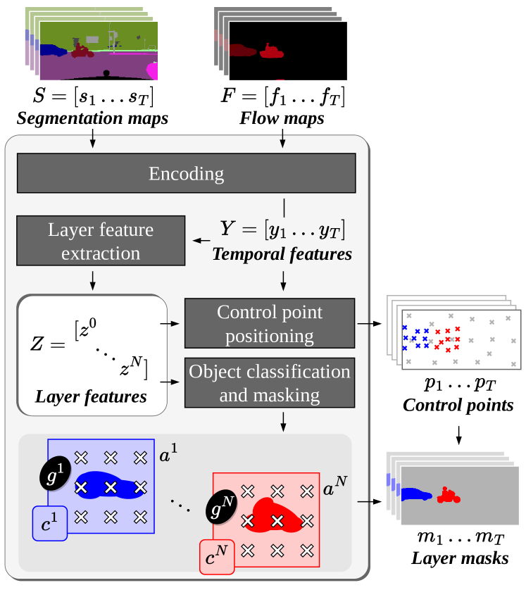
Figure 3: Layered video decomposition. Semantic and motion cues are mapped to temporal features with a time-independent encoder. These are combined to form layer features representing the background and the objects for the whole video. The position of individual layers at each time step is determined by a sparse set of control points, predicted from temporal features and layer features. We further associate with the layers a soft mask and a semantic class which are combined with the information of position to produce layer masks, segmenting the objects from the background.

3.1.1 Architecture

Input encoding.

Input flow maps and segmentation maps $F$ and $S$ are fed to a time-independent encoder, implemented by a convolutional neural network (CNN) which outputs temporal feature maps $Y=[y_{1},\ldots,y_{T}]$. Each map $y_{t}$ lies in $\mathbb{R}^{d\times h\times w}$ with feature dimension $d$ and downscaled spatial resolution $h\times w$ such that $hw\ll HW$. We denote by $l=hw$ the latent feature size, and reshape feature $y_{t}$ to an $l\times d$ matrix through raster-scan reordering.

Layer feature extraction.

We form layer features $Z=[z^{0},\ldots,z^{N}]$ from temporal ones $Y$, where, for each layer, $z^{i}$ is an $l^{i}\times d$ matrix with $l^{i}=h^{i}w^{i}$. We implement this with a transformer [83], where self-attention is replaced by a binding mechanism, discovering object-centric features by iteratively grouping intra-object pixels together, as in [54].

Control point positioning.

We add a third dimension to the control points $p_{t}^{i}$ positioned in the frame $x_{t}$ to record the corresponding layer “depth” ordering $o_{t}^{i}{\geq}0$, with $o_{t}^{i}{=}0$ for the background. In practice, the 3D vectors associated with the points $p_{t}$ are once again predicted by a transformer, from the set $Z$ of layer features and the temporal feature $y_{t}$, thus accounting for possible interactions between layers. Control points are typically close to the associated objects, but it is still fine if some end up outside an object mask. Their role is to recover a dense deformation field through TPS interpolation, and what matters is only that the part of this field within the object mask is correct. Figure 1 shows grids of control points extracted by our approach. Note how their structure automatically adapts to fit precise motions.

Layer mask prediction.

A CNN maps layer features $z^{i}$ onto soft masks $a^{i}$ with values in $[0,1]$ corresponding to opaqueness and defined in their own “intrinsic” coordinate systems, in which points associated with $p_{t}^{i}$ lie on a regular grid $g^{i}$. The background is fully opaque ($a^{0}{=}\mathbf{1}$). At time $t$, $a^{i}$ is warped onto the corresponding layer mask $m_{t}^{i}$ using the TPS transformation $w_{t}^{i}$ mapping the grid points of $g^{i}$ onto their positions $p_{t}^{i}$ in frame $x_{t}$. We then improve object contours by semantic refinement using segmentation maps $S$. Concretely, given a mask $m_{t}^{i}$ corresponding to an object layer ($i{>}0$), a soft class assignment $c^{i}$ in $[0,1]^{C}$ is obtained from $z^{i}$ with a fully-connected layer, then used to update $m_{t}^{i}$ by comparing $c^{i}$ to the actual class in $s_{t}$. We finally use the ordering scores $o_{t}$ and a classical occlusion model [62, 43] to filter non-visible layer parts. More details about this process are in Appendix A-D.

3.1.2 Training procedure

The goal of the decomposition module is to discover layers whose associated masks and control points best reconstruct scene motion. We achieve this by minimizing the objective:

$$\mathcal{L}_{{d}}=\lambda_{\text{o}}\mathcal{L}_{{o}}+\lambda_{\text{f}}\mathcal{L}_{{f}}+\lambda_{\text{r}}\mathcal{L}_{{r}},$$ (1)

with an object discovery loss $\mathcal{L}_{{o}}$ to encourage objects from different layers to occupy moving foreground regions; a flow reconstruction loss $\mathcal{L}_{{f}}$ to ensure the temporal consistency of the learned decompositions; and a regularization loss $\mathcal{L}_{{r}}$. At train time, we extract layer features from the first $T$ frames, but also position layers in the $K$ subsequent ones to have a supervision signal for later stages (Secs. 3.2 and 3.3). At inference, only the first $T$ frames are used.

Object discovery.

Without ground-truth objects for training, we discover reasonable candidates using semantic and motion cues, $f_{t}$ and $s_{t}$, by positioning objects in $\mathcal{M}(s_{t},f_{t})$, a binary mask indicating foreground regions (e.g., cars) with significant motion compared to stuff regions (e.g., road), written $\mathcal{S}(s_{t})$. We get the mask $\mathcal{M}(s_{t},f_{t})$ by extrapolating the full background flow from $f_{t}$ in $\mathcal{S}(s_{t})$, and by thresholding with a constant $\tau_{m}$ the $L_{1}$ distance between background and foreground flows. The object discovery loss is:

$$\mathcal{L}_{o}=\sum_{t}(k_{s}\mathcal{S}(s_{t})-k_{m}\mathcal{M}(s_{t},f_{t}))\odot(\max\limits_{i>0}m_{t}^{i}),$$ (2)

where $k_{m}$ and $k_{s}$ are positive scalars, weighting the attraction of discovered objects $m_{t}^{i>0}$ towards moving foreground regions ($\mathcal{M}$) and the repulsion from stuff regions ($\mathcal{S}$).

Flow reconstruction.

We reconstruct the backward flow $w_{{t_{2}}\leftarrow{t_{1}}}$ between consecutive time steps $t_{1}$ and $t_{2}$, by considering the individual layer warps, denoted $w_{{t_{2}}\leftarrow{t_{1}}}^{i}$ and computed as $w_{t_{2}}^{i}\circ w_{t_{1}}^{i}{}^{-1}$ where $w_{t_{1}}^{i}$ and $w_{t_{2}}^{i}$ are obtained through the TPS transformation associated with $p_{t_{1}}^{i}$ and $p_{t_{2}}^{i}$. We recover $w_{{t_{2}}\leftarrow{t_{1}}}$ by compositing layer warps, i.e., $w_{{t_{2}}\leftarrow{t_{1}}}=\sum_{i}{m_{t_{2}}^{i}\odot{w^{i}_{{t_{2}}\leftarrow{t_{1}}}}}$, where the mask $m_{t_{2}}^{i}$ determines layer transparency. The flow reconstruction loss is:

$$\mathcal{L}_{{f}}=\sum_{t}\|f_{t}-\hat{f}_{t}\|_{1},\,\,\text{with}\,\,\,\,\hat{f}_{t}=w_{t\leftarrow{t-1}}.$$ (3)

Regularization.

The last objective $\mathcal{L}_{{r}}$ is composed of: an entropy term applied to layer mask $m_{t}$ to ensure that a single layer prevails for every pixel, and an object initialization term which is the $L_{2}$ distance from regions of interest $\mathcal{M}(s_{t},f_{t})$ which are still empty (as per $m_{t}^{i>0}$) to the control points $p_{t}^{i}$ of the nearest object (${i{>}0}$).

3.2 Future layer prediction

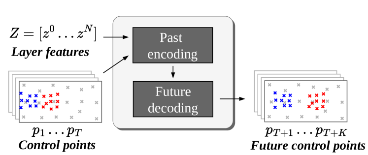
Figure 4: Future layer prediction. We encode past control point positions and object-specific knowledge (e.g., shape and semantics) in the form of layer features to produce future positions.

Thanks to our layered video decomposition, the prediction of future layers (Figure 4) is reduced to inferring, from past control points $[p_{1},\ldots,p_{T}]$, the position of future ones.

Architecture.

For each time step $t{\leq}T$ and each layer $i$, $p_{t}^{i}$ is mapped onto a vector in $\mathbb{R}^{d}$ by a linear layer. Likewise, each $z^{i}$ is also mapped onto a vector in $\mathbb{R}^{d}$. We concatenate and feed these vectors to a two-stage transformer to construct representations for the $K$ future time steps by combining self-attention modules applied to intermediate future representations and cross-attention modules between past and future ones. The prediction of the control points $p_{t}^{i}$ associated with each layer in the $K$ future time steps is done with a linear layer, which does not output their position directly, but rather their displacement with respect to $p_{T}$, with $T$ being the last known time step from the past context.

Training procedure.

We extract training data for past and future time steps by decomposing videos of length $T{+}K$ as described in Sec. 3.1. We then mask the control points corresponding to the last $K$ time steps and train the future prediction module to reconstruct them by minimizing $\mathcal{L}_{{p}}$, the $L_{1}$ distance between extracted and reconstructed control points for time steps $T{+}1$ to $T{+}K$. Under uncertainty, $\mathcal{L}_{{p}}$ makes points converge towards an average future trajectory. When interested in predicting multiple futures, we add noise (as input and in attention modules) and an adversarial term [30] to $\mathcal{L}_{{p}}$. More details are in Appendix E.

3.3 Warping, fusion and inpainting

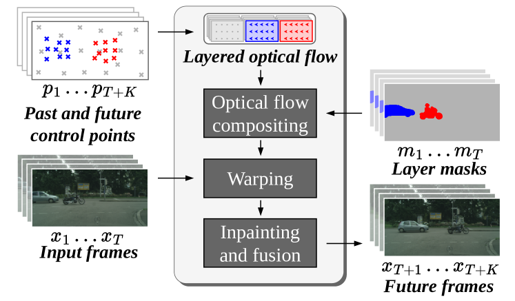
Figure 5: Warping, fusion and inpainting. From past and future control point positions we compute the warps associated with each layer and composite them to recover the dense scene flow by leveraging past layer masks for setting their transparency. We then warp frames from the past to form multiple views of future ones, merge these together, and fill in empty regions to produce final frames.

Last comes the actual synthesis of future frames from past ones (Figure 5), using the layer decompositions extracted from the past, and the ones predicted into the future.

Architecture.

Given the predicted control points, we compute, for every layer $i$ and pair of time steps $(t_{1},t_{2})$ in $\llbracket 1,T\rrbracket\times\llbracket T+1,T+K\rrbracket$, the layer warp $w^{i}_{{t_{2}}\leftarrow{t_{1}}}$ from $t_{1}$ to $t_{2}$ as described in Sec. 3.1. We construct $m_{t_{2}}^{i}$ by warping $m_{t_{1}}^{i}$ with $w^{i}_{{t_{2}}\leftarrow{t_{1}}}$. We compute $w_{{t_{2}}\leftarrow{t_{1}}}$ from layer warps and future masks by $w_{{t_{2}}\leftarrow{t_{1}}}=\sum_{i}{m_{t_{2}}^{i}\odot{w^{i}_{{t_{2}}\leftarrow{t_{1}}}}}$ as before, and warp past frames to produce multiple views of future ones, one for each pair of time steps $(t_{1},t_{2})$. We obtain $T$ views for each future frame, with different missing regions due to disocclusion. A fusion network, implemented by a U-Net [68], merges these views together according to pixel-level scores predicted for each of them. Regions which remain empty are then filled with an off-the-shelf inpainting network [51], to obtain future frame predictions $\hat{x}_{T+1}$ to $\hat{x}_{T+K}$. We ensure temporal consistency by filling frames one at a time and by using predicted motions to propagate the newly filled content onto the next frames.

Training procedure.

The inpainting model [51], trained on $8$M images from the Places dataset [111], is kept frozen and the objective to train the fusion U-Net is the weighted $L_{1}$ distance in pixel space and between features $\mathcal{F}$ extracted using the VGG [74] classification network trained on [18]:

$$\mathcal{L}_{{u}}=\sum_{t=T+1}^{T+K}\lambda_{p}\|x_{t}-\hat{x}_{t}\|_{1}+\lambda_{v}\|\mathcal{F}(x_{t})-\mathcal{F}(\hat{x}_{t})\|_{1},$$ (4)

4 Experiments

Datasets.

We train WALDO on two urban datasets, Cityscapes [17], which contains $2975$ $30$-frame video sequences for training and $500$ for testing captured at $17$ FPS, and KITTI [28], with a total of $156$ longer video sequences (${\sim}340$ frames each) including $4$ for testing. We use suitable resolutions and train / test splits for fair comparisons with prior works (setup from [7] in Table 1 and from [1] in Table 2). We also train on nonrigid scenes from UCF-Sports [67] (resp. H3.6M [41]) using the splits from [13] consisting of $6288$ sequences (resp. $73404$) for training and $752$ (resp. $8582$) for testing with roughly $10$ frames per sequence. We extract semantic and motion cues using pretrained models, namely, DeepLabV3 [14] and RAFT [77].

Evaluation metrics.

We evaluate the different methods with the multi-scale structure similarity index measure (SSIM) [94], the learned perceptual image patch similarity (LPIPS) [109], and the peak signal-to-noise ratio (PSNR), all standard image reconstruction metrics for evaluating video predictions. We also use the Fréchet video distance (FVD) [81] to estimate the gap between real and synthetic video distributions. We report in Tables 1-3 the mean and standard deviation for $3$ randomly-seeded training sessions.

Table 1: Comparison to state-of-the-art deterministic methods on Cityscapes and KITTI test sets. We compute multi-scale SSIM ($\times 10^{3}$) and LPIPS ($\times 10^{3}$) for the $k^{\text{th}}$ future frame and average for $k$ in $\llbracket 1,K\rrbracket$. We indicate if methods use semantic or flow ground truths for training.

Method Sem. Flow PredNet [55] MCNet [85] VFlow [53] VEST [110] VPVFI [100] ✓ VPCL [29] ✓ Vid2vid [90] ✓ ✓ OMP [99] ✓ ✓ SADM [7] ✓ ✓ WALDO ✓ ✓

(a) Cityscapes ($512\times 1024$) $K=1$ $K=5$ $K=10$ SSIM $\uparrow$ LPIPS $\downarrow$ SSIM $\uparrow$ LPIPS $\downarrow$ SSIM $\uparrow$ LPIPS $\downarrow$ FVD $\downarrow$   840   260   752   360   663   522     -   897   189   706   373   597   451     -   839   174   711   288   634   366     -     -     -     -     -     -     -     -   945   064   804   178   700   278   159   928   085   839   150   751   217   129   882   106   751   201   669   271     -   891   085   757   165   674   233   113   959   076   835   149     -     -     -   $\underline{957}{}_{\scriptscriptstyle\pm 2}$   $\textbf{049}_{\scriptscriptstyle\pm 1}$   $\textbf{854}_{\scriptscriptstyle\pm 1}$   $\textbf{105}_{\scriptscriptstyle\pm 1}$   $\textbf{771}_{\scriptscriptstyle\pm 1}$   $\textbf{158}_{\scriptscriptstyle\pm 1}$   $\textbf{055}_{\scriptscriptstyle\pm 1}$

(b) KITTI ($256\times 832$) $K=1$ $K=3$ $K=5$ SSIM $\uparrow$ LPIPS $\downarrow$ SSIM $\uparrow$ LPIPS $\downarrow$ SSIM $\uparrow$ LPIPS $\downarrow$ FVD $\downarrow$   563   553   514   586   475   629     -   753   240   635   317   554   373     -   539   324   469   374   426   415     -     -   156     -   344     -   447     -   827   123   695   203   611   264   050   820   172   730   220   667   259   075     -     -     -     -     -     -     -   792   185   676   246   607   304   047   831   144   724   246   647   312     -   $\textbf{867}_{\scriptscriptstyle\pm 1}$   $\textbf{108}_{\scriptscriptstyle\pm 1}$   $\textbf{766}_{\scriptscriptstyle\pm 4}$   $\textbf{163}_{\scriptscriptstyle\pm 2}$   $\textbf{702}_{\scriptscriptstyle\pm 6}$   $\textbf{206}_{\scriptscriptstyle\pm 3}$   $\textbf{042}_{\scriptscriptstyle\pm 2}$

OMP [99]	VPCL [29]	VPVFI [100]	WALDO	Ground truth

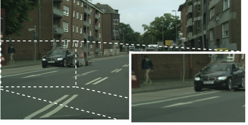
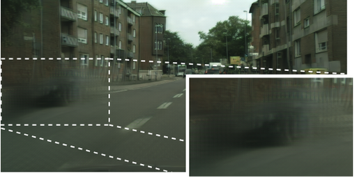
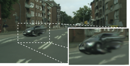
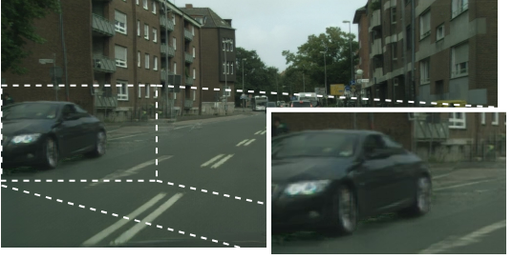
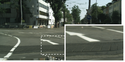
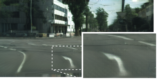
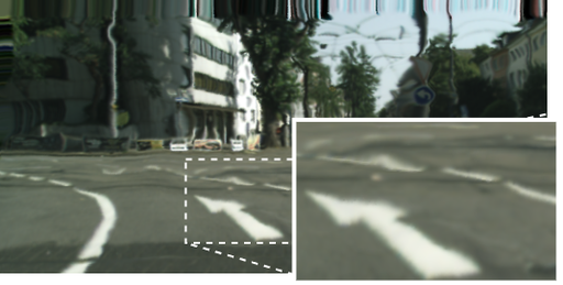
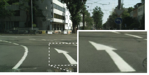
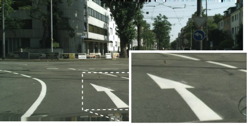
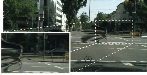
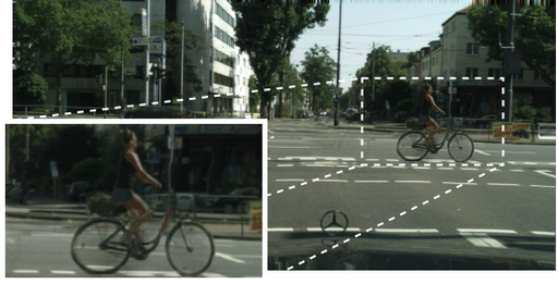
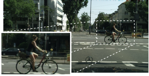
Figure 6: Comparison with [99, 29, 100] on the Cityscapes test set at time step $T{+}10$. WALDO better extracts objects from the background, better predicts their motion, and is more robust to occlusion. We strongly encourage readers to watch videos in the project webpage.

Table 2: Comparison to state-of-the-art stochastic methods (“†”) on $20$-frame future prediction on Cityscapes and KITTI. We report the best SSIM ($\times 10^{3}$), PSNR ($\times 10$), and LPIPS ($\times 10^{3}$) out of $100$ trajectories sampled from each test sequence (except for our deterministic variant). We use $4$ frames as input but others use $10$.

Method SVG† [19] SRVP† [25] HierVRNN† [11] SLAMP† [1] SLAMP-3D† [2] WALDO WALDO†

(a) Cityscapes ($128\times 256$) SSIM $\uparrow$ PSNR $\uparrow$ LPIPS $\downarrow$ $606_{\scriptscriptstyle~{}~{}~{}~{}}$ $204_{\scriptscriptstyle~{}~{}~{}~{}}$ $340_{\scriptscriptstyle~{}~{}~{}~{}}$ $603_{\scriptscriptstyle~{}~{}~{}~{}}$ $210_{\scriptscriptstyle~{}~{}~{}~{}}$ $447_{\scriptscriptstyle~{}~{}~{}~{}}$ $618_{\scriptscriptstyle~{}~{}~{}~{}}$ $214_{\scriptscriptstyle~{}~{}~{}~{}}$ ${260}_{\scriptscriptstyle~{}~{}~{}~{}}$ $\underline{649}_{\scriptscriptstyle~{}~{}~{}~{}}$ ${217}_{\scriptscriptstyle~{}~{}~{}~{}}$ $294_{\scriptscriptstyle~{}~{}~{}~{}}$ $643_{\scriptscriptstyle~{}~{}~{}~{}}$ $214_{\scriptscriptstyle~{}~{}~{}~{}}$ $306_{\scriptscriptstyle~{}~{}~{}~{}}$ ${638}_{\scriptscriptstyle\pm 1}$ $\underline{220}{}_{\scriptscriptstyle\pm 1}$ $\underline{158}{}_{\scriptscriptstyle\pm 1}$ $\textbf{653}_{\scriptscriptstyle\pm 1}$ $\textbf{224}_{\scriptscriptstyle\pm 1}$ $\textbf{147}_{\scriptscriptstyle\pm 1}$

(b) KITTI ($92\times 310$) SSIM $\uparrow$ PSNR $\uparrow$ LPIPS $\downarrow$ $329_{\scriptscriptstyle~{}~{}~{}~{}}$ $127_{\scriptscriptstyle~{}~{}~{}~{}}$ $594_{\scriptscriptstyle~{}~{}~{}~{}}$ $336_{\scriptscriptstyle~{}~{}~{}~{}}$ $134_{\scriptscriptstyle~{}~{}~{}~{}}$ $635_{\scriptscriptstyle~{}~{}~{}~{}}$ ${379}_{\scriptscriptstyle~{}~{}~{}~{}}$ ${142}_{\scriptscriptstyle~{}~{}~{}~{}}$ ${372}_{\scriptscriptstyle~{}~{}~{}~{}}$ ${337}_{\scriptscriptstyle~{}~{}~{}~{}}$ ${135}_{\scriptscriptstyle~{}~{}~{}~{}}$ $537_{\scriptscriptstyle~{}~{}~{}~{}}$ ${383}_{\scriptscriptstyle~{}~{}~{}~{}}$ ${143}_{\scriptscriptstyle~{}~{}~{}~{}}$ $501_{\scriptscriptstyle~{}~{}~{}~{}}$ $\underline{410}{}_{\scriptscriptstyle\pm 1}$ $\underline{145}{}_{\scriptscriptstyle\pm 1}$ $\underline{348}{}_{\scriptscriptstyle\pm 1}$ $\textbf{418}_{\scriptscriptstyle\pm 2}$ $\textbf{147}_{\scriptscriptstyle\pm 1}$ $\textbf{340}_{\scriptscriptstyle\pm 2}$

SLAMP [1]
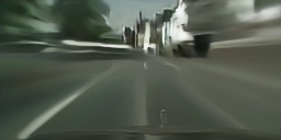
WALDO
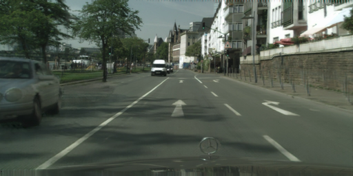
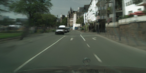
	$T+10$	$T+50$

Figure 7: Comparison to SLAMP [1] on 50-frame prediction on the Cityscapes test set. See project webpage for videos.

(a) UCF-Sports ($512\times 512$)						(a) H3.6M ($1024\times 1024$)
STRPM [13]		WALDO				STRPM [13]		WALDO
$T{+}1$	$T{+}10$	$T{+}1$	$T{+}10$	Warp		$T{+}1$	$T{+}10$	$T{+}1$	$T{+}10$	Warp

Figure 8: Future prediction comparisons to STRPM [13] from $T{=}4$ frames on (a) UCF-Sports and (b) H3.6M. In our case, nonrigid motions can be visualized by the associated warps, predicted from the control points between $T$ and $T{+}10$ (colors represent different directions).

Implementation details.

For reproducibility, code and pretrained models are available on our project webpage. WALDO is trained with the ADAM optimizer [45] and a learning rate of $10^{-4}$ on $4$ NVIDIA V100 GPUs for about a week. We set $(\lambda_{o},\lambda_{f},\lambda_{r},\lambda_{p},\lambda_{v}){=}(1,100,1,1,1)$, $(k_{s},k_{m}){=}(0.25,1)$ and $\tau_{m}{=}0.005$ by validating the performance on a random held-out subset of the training data. For example, we use spatial resolutions of $128\times 256$ for training (a) the layered video decomposition, and (b) the future layer prediction module; and $512\times 1024$ for training (c) the compositing/inpainting module on Cityscapes. As in prior works [29, 7, 99, 90], we use a context of $T{=}4$ past frames. We set the feature vector size to $d=512$. In (a), the encoder extracts one such vector for each $16\times 16$ patch from the input. The grids $g^{i}$ of resolution $4\times 4$ for each of the $N{=}16$ object layers and $8\times 16$ for the background add up to a total of $N_{c}{=}384$ control points. More details are in Appendix F.

4.1 Evaluation with the state of the art

Deterministic prediction.

WALDO sets a new state of the art on two urban datasets. On Cityscapes (Table 1(a)), it yields a better than 27% relative gain for LPIPS across all predicted time windows, and a significant margin for $K{>}1$ with SSIM and FVD. On KITTI (Table 1(b)), WALDO outperforms prior methods in a quite challenging setting, with a frame rate half that of Cityscapes and a quality of precomputed semantic and motion cues poorer on KITTI. Comparisons with latest methods [99, 29, 100] on Cityscapes (Figure 6) show that WALDO successfully models complex object (e.g., cars, bikes) and background (e.g., road markings) motions with realistic and temporally coherent outputs, whereas others produce stationary or blurry videos.

Table 3: Comparison with methods designed for nonrigid motions. We compute PSNR ($\times 10$), LPIPS ($\times 10^{3}$) for the $k\textsuperscript{th}$ future frames synthesized from 4 past ones on UCF-Sports and H3.6M test sets.

Method BMSE [58] PRNN [93] PRNN++ [91] SAVP [49] SV2P [4] HFVP [84] ELSTM [92] CGAN [48] CrevNet [108] MRNN [98] STRPM [13] WALDO

(a) UCF-Sports ($512\times 512$) PSNR $\uparrow$ LPIPS $\downarrow$ $k{=}1$ $k{=}6$ $k{=}1$ $k{=}6$ ${264}$ ${185}$ ${290}$ ${553}$ ${272}$ ${197}$ ${281}$ ${553}$ ${273}$ ${197}$ ${268}$ ${568}$ ${274}$ ${199}$ ${255}$ ${499}$ ${274}$ ${200}$ ${259}$ ${513}$   -   -   -   - ${280}$ ${203}$ ${251}$ ${478}$ ${280}$ ${200}$ ${229}$ ${449}$ ${282}$ ${203}$ ${239}$ ${481}$ ${277}$ ${200}$ ${242}$ ${492}$ $\underline{285}$ $\underline{206}$ $\underline{207}$ $\underline{411}$ $\textbf{292}_{\scriptscriptstyle\pm 2}$ $\textbf{235}_{\scriptscriptstyle\pm 1}$ $\textbf{090}_{\scriptscriptstyle\pm 1}$ $\textbf{183}_{\scriptscriptstyle\pm 1}$

(b) H3.6M ($1024\times 1024$) PSNR $\uparrow$ LPIPS $\downarrow$ $k{=}1$ $k{=}4$ $k{=}1$ $k{=}4$   -   -   -   - $319$ $257$ $126$ $140$ $321$ $275$ $138$ $150$   -   -   -   - $319$ $273$ $139$ $150$ $321$ $273$ $134$ $145$ $324$ $277$ $131$ $139$ $328$ $283$ $102$ $110$ $332$ $283$ $115$ $124$ $322$ $280$ $121$ $133$ $\underline{333}$ $\underline{290}$ $\underline{097}$ $\underline{104}$ $\textbf{363}_{\scriptscriptstyle\pm 3}$ $\textbf{314}_{\scriptscriptstyle\pm 1}$ $\textbf{058}_{\scriptscriptstyle\pm 2}$ $\textbf{071}_{\scriptscriptstyle\pm 1}$

Stochastic prediction.

We adapt WALDO to the prediction of multiple futures by injecting noise inputs to the layer prediction module and using (at train time only) a discriminator to capture multiple modes of the distribution of synthetic trajectories. This simple procedure results in significant improvements in the stochastic setting (Table 2). In particular, WALDO outperforms other stochastic methods on the same datasets by a large margin. Interestingly, even our deterministic variant compares favourably to these approaches. Minimizing the $L_{1}$ reconstruction error (in this variant) make predictions average over all possible futures. Because we predict positions and not pixel values directly, and since averaging still yields valid positions, we obtain sharp images. On the other hand, averaging over pixels inevitably blur them out. This critical distinction is illustrated in Table 4(e). Although the loss function introduced in VPCL [29] aims at sharpening pixel predictions, the examples in Figure 6 show that WALDO is more successful.

Long-term prediction.

WALDO produces arbitrary long videos, without additional training, when used in an autoregressive mode. In $20$-frame prediction (Table 2), it significantly outperforms prior works, without using its full potential since a lower resolution is used to match those of other methods. Visual comparisons with SLAMP [1]⁴ (Figure 7) at full resolution on 50-frame prediction (longer than the 30-frame videos in Cityscapes) are also striking.

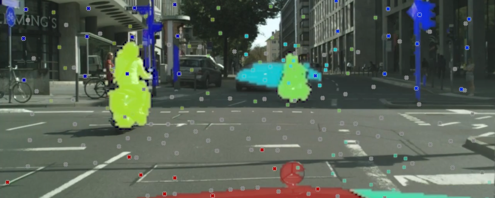
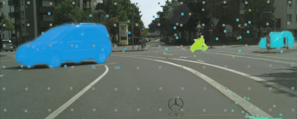
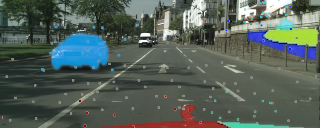
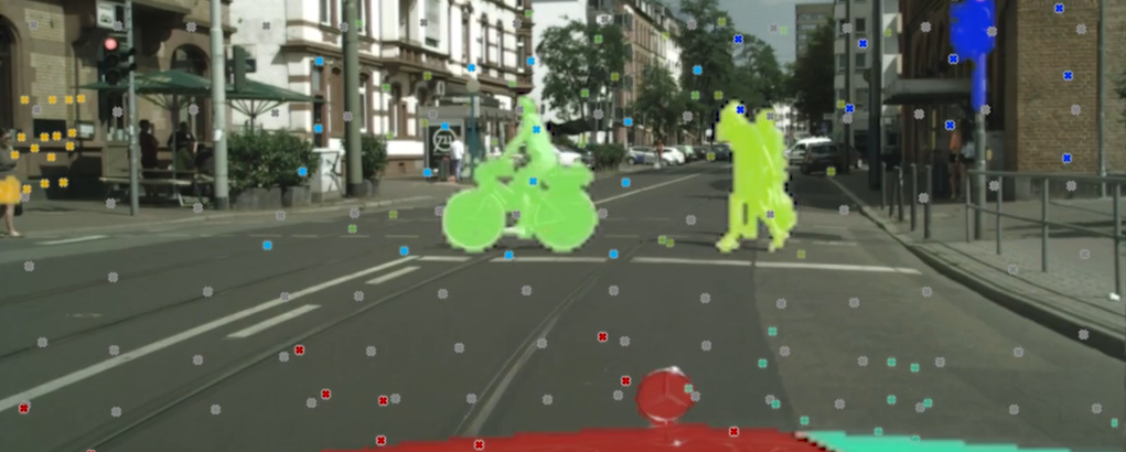
Figure 9: Visualization of control points and layer masks with different colors for each layer. See project webpage for videos.

Table 4: Ablation study on the Cityscapes test set. (a) Layered video decomposition: We evaluate decompositions in terms of flow reconstruction and object discovery as captured by $\mathcal{L}_{f}$ and $\mathcal{L}_{o}$. (b) Future layer prediction: We measure the accuracy of predicted control points. (c) Video synthesis: We evaluate the image reconstruction quality. (d) An example without (left) and with (right) semantic refinement. (e) $L_{1}$ reconstructions of an image in pixel space (left) and using control points (right) assuming Gaussian uncertainty over the horizontal position of the object. The former is blurry due to the plurality of potential positions. The latter singles out one position and preserves the object appearance.

(a) Layered video decomposition. $N$ Input Ref. $N_{c}$ $\mathcal{L}_{f}$ $\downarrow$ $\mathcal{L}_{o}$ $\downarrow$ 0 $X$ 128 4.42  0.00 1 $X$ 144 6.06 -3.69 8 $X$ 256 4.47 -5.96 16 $X$ 384 3.97 -5.79 16 $S$ 384 3.90 -7.59 16 $S{+}F$ 384 2.69 -7.56 16 $S{+}F$ ✓ 24 7.44  0.00 16 $S{+}F$ ✓ 72 7.01 -3.26 16 $S{+}F$ ✓ 176 4.17 -4.78 16 $S{+}F$ ✓ 288 3.16 -7.93 16 $S{+}F$ ✓ 384 2.59 -8.16

(b) Future layer prediction. Arch. Input $\Delta p_{T}$ $\mathcal{L}_{p}$ $\downarrow$ MLP $P$ .514 T $P$ .178 T $P$ ✓ .150 T $P{+}Z$ ✓ .144 (c) Video synthesis. VGG HR Ctxt. SSIM $\uparrow$ 1 812.1 ✓ 1 815.7 ✓ ✓ 1 847.2 ✓ ✓ 4 848.0

(d) Semantic refinement.		(e) Prediction strategy.

Nonrigid prediction.

To show that WALDO can handle complex motions, we retrain it on data with significant nonrigid objects, namely UCF-Sports and H3.6M datasets. Since our approach relies on TPS transformations, it can represent arbitrarily nonrigid motions when the number of control points is set accordingly [9]. By increasing the total number of per object points from $16$ to $64$, WALDO produces realistic videos even for deformable bodies such as human beings (Figure 8). As highlighted by the predicted warps, it successfully handles fine-grained motions covering a variety of human activities such as weight-lifting, doing gymnastics, walking sideways or leaning forward. Moreover, WALDO yields much more realistic outputs than STRPM [13]⁴ by producing high quality frames longer into the future and with much less synthesis artifacts. This is confirmed by quantitative evaluations on both datasets (Table 3), with large relative improvements over the state of the art ranging from $1$ to $3$dB in PSNR and 31 to 56% in LPIPS.

	$T+1$	$T+10$	$T+1$	$T+10$
Real frame
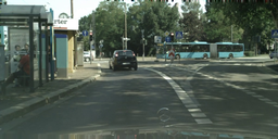
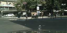
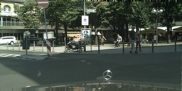
Reconstructed motion
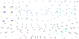
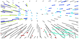
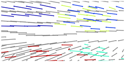
Predicted motion

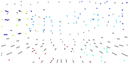
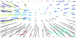
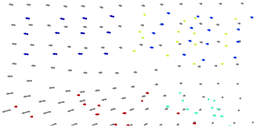
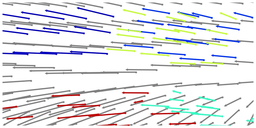
Figure 10: Visualization of future layer prediction. We use control points from the layered video decomposition as supervision. We compare motion vectors reconstructed from these points to the ones predicted for up to time step $T+10$ from a context of $T{=}4$ past frames. The motion vectors are computed between time step $T$ and time step $t$ in $\{T+1,T+10\}$. Different colors correspond to different layers.

Warped regions
Inpainted regions

Figure 11: Visualization of the synthesis process: warped visible regions and inpainted disoccluded ones between $T$ and $T{+}10$.

4.2 Ablation studies

We conduct a detailed analysis on the Cityscapes test set to compare and highlight the key novelties of WALDO. The set of hyperparameters validated through this study have proven to work well on other datasets without any tuning.

Layered video decomposition

is illustrated in Figure 9 and evaluated in Table 4(a) through the lens of our object discovery criterion ($\mathcal{L}_{o}$) and flow reconstruction ($\mathcal{L}_{f}$). We observe that the more object layers ($N$) the better, except for $N{=}1$ where fitting multiple objects with a single layer is suboptimal. Comparing inputs, we find using segmentation maps ($S$) better than RGB frames ($X$) alone for object discovery, and that using flow maps ($F$) helps motion reconstruction. Semantic refinement (Ref.) yields further gains, especially to segment thin objects like traffic lights, see Table 4(d). Finally, increasing the number of control points ($N_{c}$) allows us to capture finer motions, so we use as much as fits into memory (384 per time step). Our motion representation is scalable, with parameter size reduced from a quadratic ($TK$) to a linear ($T{+}K$) dependency on time compared to methods relying on optical flow directly.

Future layer prediction

is illustrated in Figure 10 and evaluated in Table 4(b) in terms of trajectory reconstruction. Our baseline is a multi-layer perceptron (MLP), which maps past control points $P{=}\{p_{t}\}_{t=1}^{T}$ to future ones. Our actual architecture relies on a transformer (T) [83], which performs much better. Further gains are obtained by not predicting control points directly but rather their relative position ($\Delta p_{T}$) with respect to time step $T$, and by using layer features $Z{=}\{z^{i}\}_{i=0}^{N}$ as input.

Warping, fusion and inpainting

is illustrated in Figure 11 and evaluated in Table 4(c) in terms of SSIM. Control points, obtained by the layer decomposition module, are used to warp, fuse and inpaint different views of the past frames to reconstruct future ones. We find using the feature distance (VGG) to be slightly better than the pixel one alone. The flexibility of WALDO, which trains at low resolution ($128\times 256$) but produces dense motions well suited for high resolution (HR) inputs ($512\times 1024$), results in higher SSIM than keeping the same resolution than for training during inference. We further improve SSIM by warping not only one but all of the four past context frames (Ctxt.).

Off-the-shelf models.

We compare standard approaches in Appendix H, and find that WALDO is robust to the choice of the pretrained segmentation [14, 70, 15] and optical flow models [77, 76]. We also show in Appendix I that although we use an inpainting method [51] pretrained on external data [111] to produce realistic outputs in filled-in regions, it does not provide quantitative advantage to WALDO with at best marginal improvements in SSIM, LPIPS and FVD.

5 Conclusion

We have introduced WALDO, an approach to video synthesis which automatically decomposes frames into layers and relies on a compact representation of motion to predict their future deformations. Our method outperforms the state of the art for video prediction on various datasets. Future work includes exploring extensions of WALDO for applications from motion segmentation to video compression.

Limitations.

Our performance depends on the accuracy of the layer decomposition. Failure cases include objects moving in different directions but merged into the same layer, or segmentation failures, where parts of an object are missed.

We present the following items in the Appendix:

• The thin-plate splines warp computation (Section A) and its inverse (Section B)

• The detailed formulation for the semantics-aware refinement step (Section C)

• The layer occlusion model (Section D)

• A stochastic extension of our method (Section E)

• Detailed architectural choices for each of WALDO’s modules (Section F)

• More qualitative samples on nonrigid scenes (Section G)

• The influence of the choice of the pretrained segmentation and optical flow models (Section H)

• An ablation study of our inpainting strategy (Section I)

• Further information about our implementation and the overall training process (Section J)

• A statement about the societal impact of this project (Section K)

• A qualitative study of our approach (Section L)

Appendix A Thin-plate splines warp computation

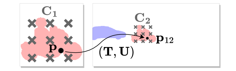
Figure A1: Thin-plate splines transformation mapping points from $\mathbf{C_{1}}$ onto $\mathbf{C_{2}}$ applied to an arbitrary point $\mathbf{p}$ using parameters ($\mathbf{T}$, $\mathbf{U}$).

For clarity, vectors (or points) are denoted by bold face lower case letters, and matrices are denoted by bold face upper case letters throughout this presentation. Let $\mathbf{p}=(x,y,1)^{\intercal}$ be a point in homogeneous coordinates, and $\mathbf{C_{1}}$ and $\mathbf{C_{2}}$ be two sets of such points in $\mathbb{R}^{3\times L}$, which we refer to as control points, with $L$ the (fixed) number of points in each set. The thin-plate splines (TPS) [9] transformation which maps $\mathbf{p}$ onto $\mathbf{p_{12}}$ writes:

$$\mathbf{p_{12}}=\mathbf{T}\mathbf{p}+\mathbf{U}\bm{\phi}(\mathbf{p},\mathbf{C_{1}}),$$ (5)

where $\bm{\phi}(\mathbf{p},\mathbf{C_{1}})=[k(\mathbf{p},\mathbf{p_{1}})]_{\mathbf{p_{1}}\in\mathbf{C_{1}}}$ is a $L$-dimensional vector, and ($\mathbf{T}$, $\mathbf{U}$) are TPS parameters in the form of matrices of dimension $3\times 3$ and $3\times L$ respectively. The transformation is decomposed into a global affine one (through $\mathbf{T}$) and a local non-affine one (through $\mathbf{U}$ and $\bm{\phi}$). The kernel function $k$ is defined by $k:(\mathbf{p},\mathbf{q})\rightarrow\|\mathbf{p}-\mathbf{q}\|_{2}^{2}\log\|\mathbf{p}-\mathbf{q}\|_{2}$ and materializes the fact that the TPS transformation minimizes the bending energy. The $3(3+L)$ TPS parameters are found using the constraint that points from $\mathbf{C_{1}}$ should be mapped onto points from $\mathbf{C_{2}}$ using (5). This yields a system of $3L$ equations to which Bookstein adds $9$ extra ones, as explained in [9], which we formulate as:

$$\mathbf{C_{1}}\mathbf{U}^{\intercal}=\mathbf{0_{3\times 3}}.$$ (6)

By applying (5) on pairs of points from $\mathbf{C_{1}}$ and $\mathbf{C_{2}}$, and using extra constraints (6), we obtain the TPS parameters ($\mathbf{T}$, $\mathbf{U}$):

$$\begin{bmatrix}\mathbf{T}^{\intercal}\\ \mathbf{U}^{\intercal}\end{bmatrix}=\bm{\Delta}(\mathbf{C_{1}})^{-1}\begin{bmatrix}\mathbf{C_{2}}^{\intercal}\\ \mathbf{0_{3\times 3}}\end{bmatrix},\,\,\,\,\,\,\,\,\,\,\bm{\Delta}(\mathbf{C_{1}})=\begin{bmatrix}\mathbf{C_{1}}^{\intercal}&\bm{\Phi}(\mathbf{C_{1}},\mathbf{C_{1}})\\ \mathbf{0_{3\times 3}}&\mathbf{C_{1}}\end{bmatrix},$$ (7)

where $\bm{\Phi}(\mathbf{C_{1}},\mathbf{C_{1}})$ is a $L\times L$ matrix obtained by stacking $\bm{\phi}(\mathbf{p_{1}},\mathbf{C_{1}})$ for all points $\mathbf{p_{1}}$ in $\mathbf{C_{1}}$.

Hence, computing the TPS parameters amounts to inverting a $(L+3)\times(L+3)$ matrix, $\bm{\Delta}(\mathbf{C_{1}})$. Since doing that for each new transformation is impractical, we use a fixed grid of control points associated with each layer for $\mathbf{C_{1}}$, as a proxy to compute the flow between pair of frames. By fixing the value of $\mathbf{C_{1}}$, the corresponding matrix inversion is done only once for the whole training; and we are still able to model different deformations by setting $\mathbf{C_{2}}$ to different values. We note that, once $\bm{\Delta}(\mathbf{C_{1}})^{-1}$ has been computed, sampling the warp $w$ associated with a new $\mathbf{C_{2}}$ is done by finding the corresponding TPS parameterization using (5), and by sampling the deformations for each point $\mathbf{p}$ in a dense grid $\llbracket 1,H\rrbracket\times\llbracket 1,W\rrbracket$ using (7), where the spatial resolution $H\times W$ can be arbitrarily large. Moreover, this process is fully differentiable with respect to $\mathbf{C_{2}}$ and each point $\mathbf{p}$ as it involves simple algebraic operations. In the main paper, $\mathbf{C_{1}}$ and $\mathbf{C_{2}}$ correspond to the regular grid of control points $g^{i}$, associated with layer $i$, and its deformation $p_{t}^{i}$ at time step $t$ respectively. The warp $w_{t}^{i}$, also in the main paper, corresponds to the inverse transformation to the one presented here, and associates with every point $\mathbf{p_{12}}$ corresponding to a pixel of the image (right side in Figure A1) the corresponding point $\mathbf{p}$ in object coordinates (left side). However, computing the inverse transformation cannot be achieved by simply switching the roles of $\mathbf{C_{1}}$ and $\mathbf{C_{2}}$, since $\mathbf{C_{1}}$ have to be kept constant, which is why we resort to warp inversion whose simple formulation is detailed in the next section.

Appendix B Inverse warp computation

Let $w$ be a warp in $\mathbb{R}^{2\times H\times W}$ (where $H\times W$ is a given spatial resolution), which we could also consider as a mapping from $\mathbb{R}^{2}$ to $\mathbb{R}^{2}$, where $w(p)$ is the geometric transformation of a point $p$ sampled on the grid $\llbracket 1,H\rrbracket\times\llbracket 1,W\rrbracket$. Such a mapping is not surjective with respect to the grid, that is, all the cells in the grid are not necessarily reached by $w$. As a result, we approximate the inverse warp $w^{-1}$ by the pixel-accurate inversion in cells for which such a direct mapping exists and use interpolation for filling others, starting from the cardinal neighbours of already inverted cells, and iteratively filling the remaining ones. The warp $w^{-1}$ may need to point out of the grid for some cells, e.g., when an object moves out of the frame. However, this cannot be extracted from $w$ which is only defined on the grid. To avoid interpolating wrong values in these cells, we only invert $w$ in those which are close (as per a given threshold) to the ones initially reached by $w$, and make others point to an arbitrary position outside of the grid layout. Finally, the same reasons which justify that training errors can backpropagate through a spatial transformer [42] also apply here.

Appendix C Semantics-aware refinement

We now describe in more details the semantics-refinement step introduced in the main body of the paper. Let $m_{t}$ be a soft mask in $[0,1]^{H\times W}$ at a given time step $t$ in $\llbracket 1,T\rrbracket$, and $c$ be a soft class assignment in $[0,1]^{C}$, both of them predicted for the same layer, and let $s_{t}$ be an input (soft) semantic map in $[0,1]^{C\times H\times W}$ also associated with time step $t$. We denote by $\bar{c}$, the mean semantic class on the spatio-temporal tube defined by the masks, which, like $c$, is a vector in $[0,1]^{C}$, and writes:

$$\bar{c}=\sum_{t,h,w}[m_{t}\odot\mathcal{F}(s_{t},c)]_{(h,w)}/\sum_{t,h,w}[m_{t}]_{(h,w)},$$ (8)

where $\odot$ is the element-wise product, and $\mathcal{F}$ is a class-filtering function parameterized by $c$ and applied to $s_{t}$, that is, at a given spatial location $(h,w)$, the result of kipping dominant classes as per $c$ in $s_{t}$:

$$[\mathcal{F}(s_{t},c)]_{(h,w)}=\frac{1}{1+k_{c}}\sum_{j}\langle[s_{t}]_{(h,w)},c+k_{c}\rangle,$$ (9)

with $k_{c}$ a constant which defines the degree at which low scoring classes will be filtered out. One can set $k_{c}=0$ for full effect and greater values for filtering less. In practice, we fix the value of $k_{c}$ to $0.1$. Each mask $m_{t}$ is updated by computing the $L_{1}$ distance between the semantic map $s_{t}$ and the mean class $\bar{c}$ at every location $(h,w)$:

$$[m_{t}]_{(h,w)}=(1-\|[s_{t}]_{(h,w)}-\bar{c}\|_{1})[m_{t}]_{(h,w)}.$$ (10)

Appendix D Layer occlusion model

Our occlusion model is rather standard, but we include it here for completeness. Ordering scores $o_{t}$ are used to filter non-visible parts in a layer $i$ due to the presence of another layer $j$ on top of it (i.e., when $o_{t}^{i}\ll o_{t}^{j}$). The transparency $m_{t}^{i}$ of layer $i$ at time step $t$ is updated as follows:

$$m^{i}_{t}=m^{i}_{t}\odot\prod_{j\neq i}\Big{(}\mathbf{1}-\frac{o_{t}^{j}}{o_{t}^{i}+o_{t}^{j}}m_{t}^{j}\Big{)},$$ (11)

where $\odot$ is the element-wise product whose right-hand side component has values between $0$ (occluded) and $1$ (visible).

Appendix E Stochastic extension of WALDO

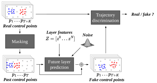
Figure E1: Stochastic future prediction. We extend the future layer prediction module of WALDO to allow the prediction of multiple futures. The module itself is not changed, except that it now uses noise (as input and in attention modules). The major difference is that a trajectory discrimination module is used at train time to assist the model in producing a realistic control point trajectory instead of the mean trajectory. At inference, only the future layer prediction module is kept. See text for details.

In our original description, motions produced by WALDO are purely deterministic and they converge towards the mean of all possible future trajectories given the past. Although it is sufficient for short-term prediction, one could be interested in modeling different behaviours for longer future horizons. For this reason, we propose an extension of WALDO to account for the intrinsically uncertain nature of the future by allowing multiple predictions.

Our approach, illustrated in Figure E1, builds upon generative adversarial networks (GANs) [30]. We consider the future layer prediction module as a generator which computes the future positions of control points given ones from the past. This generator is trained jointly with a discriminator which classifies trajectories as real or fake. Both are playing a minimax game, where the discriminator is taught to correctly distinguish real from fake trajectories, while the generator tries to fool the discriminator. Through this process we expect synthetic trajectories to gradually improve in realism and to capture multiple modes from the underlying data distribution.

We implement the discriminator with a transformer and use the WGAN loss introduced in [3] for training. In addition to this loss, we find that keeping the initial reconstruction term ($\mathcal{L}_{{p}}$) is important for the stability of training. Moreover, we normalize gradients from both supervision signals (reconstruction and adversarial) so that they have matching contributions.

Appendix F Detailed architectures

We detail inner operations of each of WALDO’s modules (for the dimensions used on Cityscapes [17]).

F.1 Layered video decomposition

Table F1: Input encoding.

Stage	Operation	On	Output size
$s$	-	-	$20\times 128\times 256$
$f$	-	-	$2\times 128\times 256$
1	Concat.	$s$, $f$	$22\times 128\times 256$
Conv1	$[3\times 3]$	1	$64\times 64\times 128$
LN1	Norm.	1	$64\times 64\times 128$
Act1	GELU	1	$64\times 64\times 128$
Conv2	$[3\times 3]$	1	$128\times 32\times 64$
LN2	Norm.	1	$128\times 32\times 64$
Act2	GELU	1	$128\times 32\times 64$
Conv3	$[3\times 3]$	1	$256\times 16\times 32$
LN3	Norm.	1	$256\times 16\times 32$
Act3	GELU	1	$256\times 16\times 32$
Conv4	$[3\times 3]$	1	$512\times 8\times 16$
$y$	-	1	$512\times 8\times 16$

Input encoding.

Semantic and flow maps ($s$ and $f$) are concatenated and go through a series of $3\times 3$ convolutional layers (Conv) with padding of $1$ and stride of $2$, each followed by layer norm (LN) and a GELU activation [35] (Act) to form downscaled features $y$ for a given time step.

Layer feature extraction.

We combine features encoded from different time steps into ($Y$), and sum them with different embeddings corresponding to their temporal ordering and spatial positioning (T and P) to form input (1). Layer features $Z_{obj}$ and $Z_{bg}$ are computed from input (2), which is the concatenation of object and background embeddings (2a and 2b), themselves expressed as the sum of layer ordering and spatial positioning embeddings (S, L, O and B). The next operations consists in layer norm (LN), self-attention (Att) to update (2) by computing queries, keys and values for (1) but only keys and values for (2), and multi-layer perceptrons (MLP) with GELU activations [35].

Control point positioning.

We apply similar operations to predict control points $(p_{obj},p_{bg})$ for object and background layers at a given time step from associated features $y$. A key difference with the previous module is that this one is time-independent, and that inputs (1) and (2) play the same role in the transformer blocks. A fully-connected layer (FC) outputs the 3D position of each control point in each of the $16+1$ layers.

Object masking.

This module predicts an alpha-transparency mask $a$ for an object from its associated features $z$. It is the reverse process compared to the input encoding module, that is, we replace convolutions with transposed ones for progressively upscaling feature maps $z$, and we decrease the size of features at each step instead of increasing it.

Object classification.

This module predicts for each object represented by $z$ a soft class assignment $c$, by first averaging $z$ over its spatial dimensions, and then applying layer norm (LN), a fully-connected layer (FC), and a softmax activation (Act) to output $c$ as a categorical distribution over classes.

F.2 Future layer prediction

Past encoding.

Past control points corresponding to objects (resp. the background) are transformed into vectors, each of them paired with one layer and one time step, using a fully-connected layer FC1 (resp. FC2). We apply a pooling operation to layer representations ($Z_{obg}$ and $Z_{bg}$) to reduce them to a single vector representing each layer. All these vectors are concatenated, summed with the suitable embeddings (T and P), and passed through two vanilla transformer blocks to produce encoded features $E$.

Future decoding.

Future control points are obtained by initializing future representations (2) with some embeddings (T and P), and then alternating between transformer blocks with self-attention on future representations (2), and cross-attention from past to future ones (1 and 2).

F.3 Warping, inpainting and fusion

The final component of our approach is a U-Net [68] composed of $6$ downscaling layers and $6$ upscaling ones, with as many skip connections between the two branches. Each downscaling (resp. upscaling) layer divides (resp. multiplies) by $2$ its input resolution using a $3\times 3$ convolution (resp. transposed convolution) with a stride of $2$, and multiplies (resp. divides) by $2$ the size of features so that intermediate features (between the two branches) are of size $512$. This module outputs RGB values to update certain regions of an image (filling missing background or object parts, adapting light effects or shadows in other parts), a mask indicating these regions, a score (of confidence) at each pixel location to allow fusing multiple views corresponding to the same image.

Table F2: Layer feature extraction.                      

Stage	Operation	On	Output size
$Y$	-	-	$4\times 512\times 8\times 16$
(T)	Embed.	-	$4\times 512\times 1\times 1$
(P)	Embed.	-	$1\times 512\times 8\times 16$
1	Sum/Reshape	$Y$, T, P	$512\times 512$
(S)	Embed.	-	$1\times 512\times 4\times 4$
(L)	Embed.	-	$1\times 512\times 8\times 16$
(O)	Embed.	-	$16\times 512\times 1\times 1$
(B)	Embed.	-	$1\times 512\times 1\times 1$
2a	Sum/Reshape	S, O	$256\times 512$
2b	Sum/Reshape	L, B	$128\times 512$
2	Concat.	2a, 2b	$384\times 512$
LN1	Norm.	1	$512\times 512$
LN2	Norm.	2	$384\times 512$
Att1	$[512]\times 3$	2/1	$384\times 512$
LN3	Norm.	2	$384\times 512$
MLP1	$[2048,512]$	2	$384\times 512$
LN4	Norm.	2	$384\times 512$
Att2	$[512]\times 3$	2/1	$384\times 512$
LN5	Norm.	2	$384\times 512$
MLP2	$[2048,512]$	2	$384\times 512$
$Z_{obj}$	Split/Reshape	2	$16\times 512\times 4\times 4$
$Z_{bg}$	Split/Reshape	2	$1\times 512\times 8\times 16$

Table F3: Control point positioning.                    

Stage	Operation	On	Output size
$y$	-	-	$512\times 8\times 16$
(P)	Embed.	-	$512\times 8\times 16$
1	Sum/Reshape	$y$, P	$128\times 512$
$Z_{obj}$	-	-	$16\times 512\times 4\times 4$
$Z_{bg}$	-	-	$1\times 512\times 8\times 16$
(S)	Embed.	-	$1\times 512\times 4\times 4$
(L)	Embed.	-	$1\times 512\times 8\times 16$
(O)	Embed.	-	$16\times 512\times 1\times 1$
(B)	Embed.	-	$1\times 512\times 1\times 1$
2a	Sum/Reshape	$Z_{obj}$, S, O	$16\times 512\times 4\times 4$
2b	Sum/Reshape	$Z_{bg}$, L, B	$1\times 512\times 8\times 16$
2	Concat.	2a, 2b	$384\times 512$
3	Concat.	1, 2	$512\times 512$
LN1	Norm.	3	$512\times 512$
Att1	$[512]\times 3$	3	$512\times 512$
LN2	Norm.	3	$512\times 512$
MLP1	$[2048,512]$	3	$512\times 512$
LN3	Norm.	3	$512\times 512$
Att2	$[512]\times 3$	3	$512\times 512$
LN4	Norm.	3	$512\times 512$
MLP2	$[2048,512]$	3	$512\times 512$
2	Split	3	$384\times 512$
FC	[3]	2	$384\times 3$
$p_{obj}$	Split/Reshape	2	$16\times 3\times 4\times 4$
$p_{bg}$	Split/Reshape	2	$1\times 3\times 8\times 16$

Table F4: Object masking.                       

Stage	Operation	On	Output size
$z$	-	-	$512\times 4\times 4$
1	-	$z$	$512\times 4\times 4$
LN1	Norm.	1	$512\times 4\times 4$
TConv1	$[3\times 3]$	1	$256\times 8\times 8$
LN2	Norm.	1	$256\times 8\times 8$
Act1	GELU	1	$256\times 8\times 8$
TConv2	$[3\times 3]$	1	$128\times 16\times 16$
LN3	Norm.	1	$128\times 16\times 16$
Act2	GELU	1	$128\times 16\times 16$
TConv3	$[3\times 3]$	1	$64\times 32\times 32$
LN4	Norm.	1	$64\times 32\times 32$
Act3	GELU	1	$64\times 32\times 32$
TConv4	$[3\times 3]$	1	$1\times 64\times 64$
Act4	Sigmoid	1	$1\times 64\times 64$
$a$	-	1	$1\times 64\times 64$

Table F5: Object classification.                      

Stage	Operation	On	Output size
$z$	-	-	$512\times 4\times 4$
1	Spatial mean	$z$	$512$
LN	Norm.	1	$512$
FC	$[20]$	1	$20$
Act	Softmax	1	$20$
$c$	-	1	$20$

Table F6: Past encoding.                      

Stage	Operation	On	Output size
$P_{obj}$	-	-	$4\times 16\times 3\times 4\times 4$
$P_{bg}$	-	-	$4\times 1\times 3\times 8\times 16$
1a	Reshape	$P_{obj}$	$4\times 16\times 48$
1b	Reshape	$P_{bg}$	$4\times 1\times 128$
FC1	[512]	1a	$4\times 16\times 512$
FC2	[512]	1b	$4\times 1\times 512$
$Z_{obj}$	-	-	$16\times 512\times 4\times 4$
$Z_{bg}$	-	-	$1\times 512\times 8\times 16$
2a	Pool/Reshape	$Z_{obj}$	$1\times 16\times 512$
2b	Pool/Reshape	$Z_{bg}$	$1\times 1\times 512$
3	Concat.	1a, 1b, 2a, 2b	$5\times 17\times 512$
(T)	Embed.	-	$5\times 1\times 512$
(P)	Embed.	-	$1\times 17\times 512$
3	Sum/Reshape	3, T, P	$85\times 512$
LN1	Norm.	3	$85\times 512$
Att1	$[512]\times 3$	3	$85\times 512$
LN2	Norm.	3	$85\times 512$
MLP1	$[2048,512]$	3	$85\times 512$
LN3	Norm.	3	$85\times 512$
Att2	$[512]\times 3$	3	$85\times 512$
LN4	Norm.	3	$85\times 512$
MLP2	$[2048,512]$	3	$85\times 512$
$E$	Reshape	3	$5\times 17\times 512$

Table F7: Future decoding.                      

Stage	Operation	On	Output size
$E$	-	-	$5\times 17\times 512$
1	Reshape	$E$	$85\times 512$
(T)	Embed.	-	$10\times 1\times 512$
(P)	Embed.	-	$1\times 17\times 512$
2	Sum/Reshape	T, P	$170\times 512$
LN1	Norm.	1	$170\times 512$
LN2	Norm.	2	$170\times 512$
Att1	$[512]\times 3$	2	$170\times 512$
LN3	Norm.	2	$170\times 512$
MLP1	$[2048,512]$	2	$170\times 512$
LN4	Norm.	2	$170\times 512$
Att2	$[512]\times 3$	2/1	$170\times 512$
LN5	Norm.	2	$170\times 512$
MLP2	$[2048,512]$	2	$170\times 512$
LN6	Norm.	2	$170\times 512$
Att3	$[512]\times 3$	2	$170\times 512$
LN7	Norm.	2	$170\times 512$
MLP3	$[2048,512]$	2	$170\times 512$
LN8	Norm.	2	$170\times 512$
Att4	$[512]\times 3$	2/1	$170\times 512$
LN9	Norm.	2	$170\times 512$
MLP4	$[2048,512]$	2	$170\times 512$
LN10	Norm.	2	$170\times 512$
2a	Split	2	$160\times 512$
2b	Split	2	$10\times 512$
FC1	[48]	2a	$160\times 48$
FC2	[384]	2b	$10\times 384$
$P_{obj}$	Reshape	2a	$10\times 16\times 3\times 4\times 4$
$P_{bg}$	Reshape	2b	$10\times 1\times 3\times 8\times 16$

Appendix G Additional visual results on nonrigid scenes

$T{+}1$	$T{+}10$	Warp	$T{+}1$	$T{+}10$	Warp

Figure G2: Future prediction from $T{=}4$ frames on Taichi-HD ($256\times 256$). Nonrigid motions can be visualized by the associated warps, predicted from the control points between $T$ and $T{+}10$ (colors represent different directions).

We further illustrate (Figure G2) that the motion representation proposed in WALDO allows us to represent nonrigid object deformations by training on Taichi-HD [73] dataset. Our approach can handle complex human motions such as leaning forward / backward, moving one leg while keeping the other on the ground, raising individual arms…

Appendix H Influence of the choice of the pretrained segmentation and optical flow models

The use of pretrained networks in prior works vary widely according to the level of information required by each method, and depending on what was available at the time to extract these information. We summarize the differences in Table H1.

Table H1: Pretrained models used by different methods.

Method	Optical flow estimation	Semantic segmentation	Instance segmentation	Depth estimation	Object tracking	Video Frame Interpolation
VPVFI [100]	RAFT [77]	-	-	-	-	RIFE [39]
VPCL [29]	RAFT [77]	-	-	-	-	-
Vid2vid [90]	FlowNet2 [40]	DeepLabV3 [14]	-	-	-	-
OMP [99]	PWCNet [76]	VPLR [113]	UPSNet [102]	GeoNet [107]	SiamRPN++[50]	-
SADM [7]	PWCNet [76]	DeepLabV3 [14]	-	-	-	-
WALDO	RAFT [77]	DeepLabV3 [14]	-	-	-	-

We thus evaluate the influence of the choice of the pretrained segmentation and optical flow models to WALDO’s performance. Results on Cityscapes and KITTI test set, obtained by substituting segmentation model DeepLabV3 [14] with MobileNetV2 [70] or ViT-Adapter [15], and optical flow model RAFT [77] with PWCNet [76], are presented in Table H2.

Table H2: Ablation studies of optical flow estimation and semantic segmentation methods on the Cityscapes and KITTI test sets. Like in the main paper, we compute multi-scale SSIM ($\times 10^{3}$) and LPIPS ($\times 10^{3}$) for the $k^{\text{th}}$ frame and report the average for $k$ in $\llbracket 1,K\rrbracket$.

Flow Segmentation [76] [77] [70] [14] [15] ✓ ✓ ✓ ✓ ✓ ✓ ✓ ✓

(a) Cityscapes $K=1$ $K=5$ $K=10$ SSIM $\uparrow$ LPIPS $\downarrow$ SSIM $\uparrow$ LPIPS $\downarrow$ SSIM $\uparrow$ LPIPS $\downarrow$ 947 062 836 122 753 175 954 055 849 111 768 165 957 049 854 105 771 158 957 $\underline{050}$ $\underline{853}$ 105 $\underline{770}$ $\underline{159}$

(b) KITTI $K=1$ $K=3$ $K=5$ SSIM $\uparrow$ LPIPS $\downarrow$ SSIM $\uparrow$ LPIPS $\downarrow$ SSIM $\uparrow$ LPIPS $\downarrow$ 856 116 760 171 697 214 859 112 756 166 692 209 867 108 $\underline{766}$ 163 $\underline{702}$ $\underline{206}$ $\underline{866}$ $\underline{109}$ 767 163 703 205

Despite PWCNet [76] having approximately twice the average end-point-error of RAFT [77], using it instead of RAFT only results in a small performance drop for video prediction with WALDO. This is in line with the conclusions of Geng et al. in [29] who conducted a similar comparison. Moreover, replacing DeepLabV3 [14] with MobileNetV2 [70], with respective segmentation performance of $81$ and $75$ in terms of test set mIoU on Cityscapes, yields only little loss of video prediction quality. Conversely, using a more advanced segmentation model like ViT-Adapter [15], with $85$ test set mIoU on Cityscapes, does not change the results substantially. Our interpretation is that the segmentation quality is not the limiting factor for WALDO’s performance once it has reached a sufficient level. To conclude, WALDO is quite robust to the choice of the pretrained segmentation and optical flow models.

Appendix I Ablation study of the inpainting strategy

Table I1: Ablation of our inpainting strategy on the Cityscapes test set.

Adversarial inpainting [51]	Temporal consistency	$K=1$		$K=5$		$K=10$
		SSIM $\uparrow$	LPIPS $\downarrow$	SSIM $\uparrow$	LPIPS $\downarrow$	SSIM $\uparrow$	LPIPS $\downarrow$	FVD $\downarrow$
		957	049	${853}$	105	${770}$	158	061
✓		957	049	854	105	771	158	$\underline{057}$
✓	✓	957	049	854	105	771	158	055

$\varnothing$
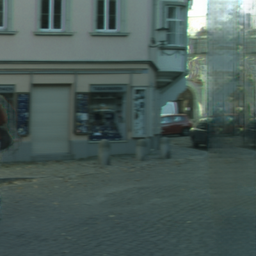
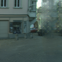
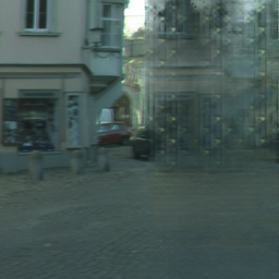
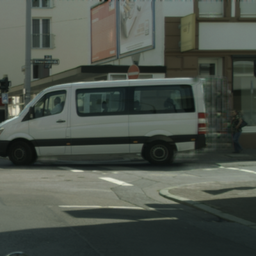
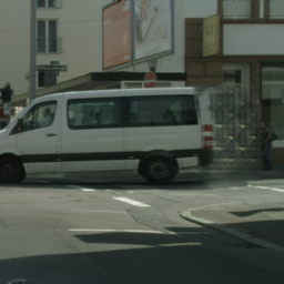
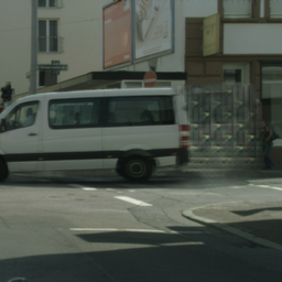
Adv. inp. [51]
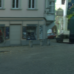
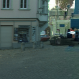
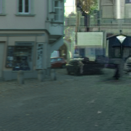
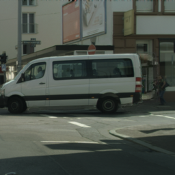
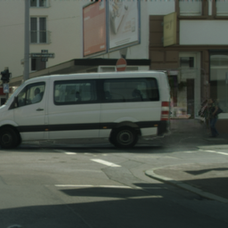
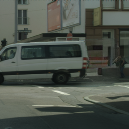
Adv. inp. [51] + Temp. cons.
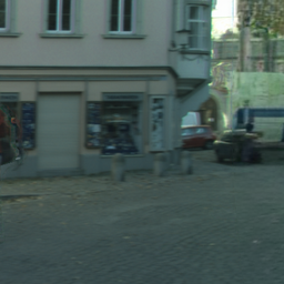
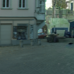
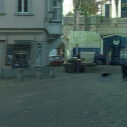
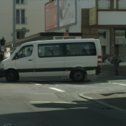
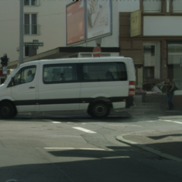
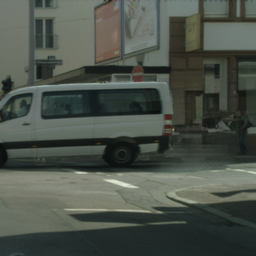
Disoccluded regions
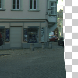
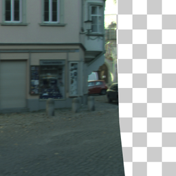
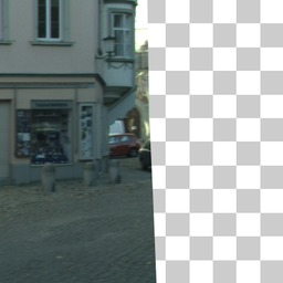
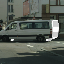
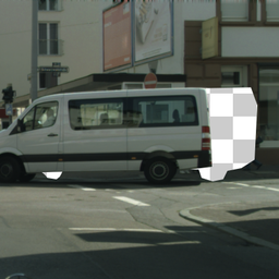
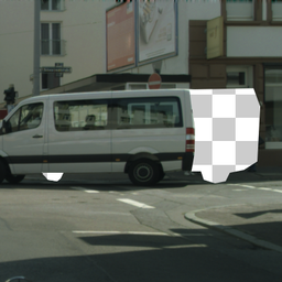
	$T+4$	$T+7$	$T+10$	$T+4$	$T+7$	$T+10$

Figure I3: Visual ablation of our inpainting strategy. We start off with a method that fills in empty regions with the sole objective to minimize the reconstruction error ($\varnothing$), we then propose to leverage an off-the-shelf adversarial inpainting (adv. inp.) method [51] to improve realism, and we finally illustrate our full strategy where we use the predicted flow to ensure the temporal consistency (temp. const.) of inpainted regions. For clarity, these regions are indicated in the last row. Please zoom in for details.

Given that we use an off-the-shelf inpainting method [51] trained on external data [111], we assess the impact of the use of such a model in our approach on quantitative measurements.

Results are presented in Table I1 and show that although gains in SSIM and FVD are possible, these gains remain small. In addition, no perceptible change is observed on LPIPS. Our temporal consistency strategy, which consists in filling frames one by one and using the predicted flow to propagate new contents into subsequent frames, allow small extra gains on the FVD metric.

The benefits from our inpainting strategy are more visible in qualitative samples presented in Figure I3. Without adversarial inpainting ($\varnothing$), empty image regions are filled using a model trained to minimize the reconstruction error. We observe that this results in blurry image parts with important artefacts. Using adversarial inpainting produces much more realistic images when considering frames individually, but filling each of them independently is still not very natural (best viewed in the videos included in the project webpage). Our approach for producing temporally-consistent outputs is able to solve this issue. For example, in the left-most sample sequence of the third row of Figure I3, we see that inpainted image parts match between different time steps although the camera is moving.

Appendix J Further implementation details

We follow [99] and group semantic classes which form a consistent entity together, e.g., riders with their bicycle, traffic lights/signs with the poles, which allows us to represent those within a single object layer. We use horizontal flips, cropping, and color jittering as data augmentation. Although we encounter signs of over-fitting in some experiments, validation curves do not increase during training, nor after convergence. So best model selection is not necessary, and we always save the last checkpoint. We find that a good initialization of object regions helps the layer decomposition module to reach a better optimum and to converge faster. Hence, we add a warmup period during which the module is trained without flow reconstruction ($\lambda_{f}=0$), and then progressively increase the associated parameter during training ($\lambda_{f}>0$) once we start having good object proposals. Without doing so, the module tends to rely on the background layer alone to reconstruct the scene motion, which, as a result, leads to an under-use of the object layers. We also find that removing data-augmentation in the last few epochs when training the warping, inpainting and fusing module slightly improves the performance at inference time.

Appendix K Societal impact

The total cost for this project, including architecture and hyperparameter search, training, testing and comparisons with baselines has been around 25K GPU hours, with an associated environmental cost of course. On the other hand, we strive to minimize this cost by decomposing video prediction into efficient lightweight modules, and our approach will hopefully contribute to eventually improve the safety of autonomous vehicles, by, say, predicting the motion of nearby agents.

Appendix L Qualitative study of WALDO

In this section, we provide qualitative samples for each of the three modules which compose WALDO.

Layered video decomposition.

We illustrate in Figure L1 our strategy to decompose videos into layers as a way to build inter-frame connections using a compact representation of motion from which we recover the dense scene flow.

	$t=1$	$t=7$	$t=14$	$t=1$	$t=7$	$t=14$
Real frame
Real seg. map
Real flow map
Pseudo objects
Rec. objects
Layer masks
Rec. motion
Rec. flow

Figure L1: Visualization of the layered video decomposition. Semantic segmentation maps and optical flow maps are extracted from RGB frames using off-the-shelf methods [14, 77]. We combine both to construct pseudo ground truths for object discovery: in white, moving foreground regions towards which objects are attracted; in grey, static foreground ones which remain neutral; and in black, the background which repulses objects. We then show predicted object regions and their decomposition into layers. Each layer is tracked over time using a small set of control points. We compute motion vectors between points in pairs of frames (here, between consecutive time steps), and reconstruct from these and the layer masks the complex scene flow. Please zoom in for details.

We observe that objects are predicted in regions which match our pseudo ground truth, constructed from input segmentation and flow maps, even in difficult regions like the poles. Although they share the same semantic class, the three cars in the left-most example in Figure L1 are correctly segmented into different objects. Still, it may happen that multiple objects are merged into the same layer, or that an object is over-segmented into multiple layers (like the ego vehicle in these examples). This is due, in part, to the limitations of our approach which indicates regions of interest for the objects, but does not impose how they should be split among the different layers. When computing video decompositions, we also position a set of control points associated with each layer. The delta of control points between pairs of time steps produces sparse motion vectors for the background and the objects. We show that, although we use a small number of points, we are able to accurately recover the dense scene flow using TPS transformations, and that motion discontinuities occur at layer boundaries as expected.

Future layer prediction.

We compare in Figure L2 the scene dynamics extracted from our decomposition strategy to the one inferred via the future layer prediction module.

	$T+1$	$T+5$	$T+10$	$T+1$	$T+5$	$T+10$
Real frame
Rec. motion
Pred. motion
Real frame
Rec. motion
Pred. motion
Real frame
Rec. motion
Pred. motion

Figure L2: Visualization of future layer prediction. We use control points from the layered video decomposition as supervision. We compare motion vectors reconstructed from these points to the ones predicted for up to time step $T+10$ from a context of $T{=}4$ past frames. The motion vectors are computed between time step $T$ and time step $t$ in $\{T+1,T+10\}$. Different colors correspond to different layers. Please zoom in for details.

We accurately reconstruct complex motions under various scenarios: when the background is static, moves towards the camera due to the ego motion, or sideways when the car is turning; in the presence of different kinds of objects such as trucks, cars, bikes or various road elements; and whether these objects move in the same direction or not.

Warping, fusion and inpainting.

We illustrate in Figure L3 how future frames are finally synthesized.

	$T+1$	$T+5$	$T+10$	$T+1$	$T+5$	$T+10$
Real frame
Warped frame
Inp. frame
Disocc.
Real frame
Warped frame
Inp. frame
Disocc.

Figure L3: Visualization of the warping, fusion and inpainting module. We use the layer decomposition computed on a whole video to reconstruct the last $10$ frames using the $T=4$ first ones as context. This is done by warping, inpainting and fusing different views from the context. We compare real frames, warped ones, and fused/inpainted ones. We also illustrate the effect of disocclusion, by showing in the last row, in black, regions which are not visible in any frame of the context, and, in grey, those which are not visible in some frames but visible in others. Please zoom in for details.

Warping past frames to obtain future ones is not enough, as some regions may not be recovered from the past. In particular, we see that shadows may not always be consistent with the new position of objects, e.g., for the vehicle in the bottom-right example in Figure L3. Our fusion and inpainting strategy is able to fill empty regions with realistic and temporal-consistent content (see also Sec I), and handles shadows reasonably well. Finally, we show that by fusing multiple views from the past context, WALDO is able to reduce disocclusions significantly (from the grey + black to only black regions in the last row of the figure).

References

- [1] Adil Kaan Akan, Erkut Erdem, Aykut Erdem, and Fatma Güney. SLAMP: Stochastic latent appearance and motion prediction. In ICCV, 2021.
- [2] Adil Kaan Akan, Sadra Safadoust, Erkut Erdem, Aykut Erdem, and Fatma Güney. Stochastic video prediction with structure and motion. arXiv preprint, 2022.
- [3] Martin Arjovsky, Soumith Chintala, and Léon Bottou. Wasserstein generative adversarial networks. In ICML, 2017.
- [4] Mohammad Babaeizadeh, Chelsea Finn, Dumitru Erhan, Roy H. Campbell, and Sergey Levine. Stochastic variational video prediction. In ICLR, 2018.
- [5] Zhipeng Bao, Pavel Tokmakov, Allan Jabri, Yu-Xiong Wang, Adrien Gaidon, and Martial Hebert. Discovering objects that can move. In CVPR, 2022.
- [6] Amir Bar, Roei Herzig, Xiaolong Wang, Anna Rohrbach, Gal Chechik, Trevor Darrell, and Amir Globerson. Compositional video synthesis with action graphs. In ICML, 2021.
- [7] Xinzhu Bei, Yanchao Yang, and Stefano Soatto. Learning semantic-aware dynamics for video prediction. In CVPR, 2021.
- [8] Serge Belongie, Jitendra Malik, and Jan Puzicha. Shape matching and object recognition using shape contexts. TPAMI, 2002.
- [9] Fred L. Bookstein. Principal warps: Thin-plate splines and the decomposition of deformations. TPAMI, 1989.
- [10] Christopher P Burgess, Loic Matthey, Nicholas Watters, Rishabh Kabra, Irina Higgins, Matt Botvinick, and Alexander Lerchner. Monet: Unsupervised scene decomposition and representation. arXiv preprint, 2019.
- [11] Lluis Castrejon, Nicolas Ballas, and Aaron Courville. Improved conditional VRNNs for video prediction. In ICCV, 2019.
- [12] Michael B Chang, Tomer Ullman, Antonio Torralba, and Joshua B Tenenbaum. A compositional object-based approach to learning physical dynamics. In ICLR, 2016.
- [13] Zheng Chang, Xinfeng Zhang, Shanshe Wang, Siwei Ma, and Wen Gao. STRPM: A spatiotemporal residual predictive model for high-resolution video prediction. In CVPR, 2022.
- [14] Liang-Chieh Chen, Yukun Zhu, George Papandreou, Florian Schroff, and Hartwig Adam. Encoder-decoder with atrous separable convolution for semantic image segmentation. In ECCV, 2018.
- [15] Zhe Chen, Yuchen Duan, Wenhai Wang, Junjun He, Tong Lu, Jifeng Dai, and Yu Qiao. Vision transformer adapter for dense predictions. arXiv preprint, 2022.
- [16] Aidan Clark, Jeff Donahue, and Karen Simonyan. Adversarial video generation on complex datasets. arXiv preprint, 2019.
- [17] Marius Cordts, Mohamed Omran, Sebastian Ramos, Timo Rehfeld, Markus Enzweiler, Rodrigo Benenson, Uwe Franke, Stefan Roth, and Bernt Schiele. The Cityscapes dataset for semantic urban scene understanding. In CVPR, 2016.
- [18] Jia Deng, Wei Dong, Richard Socher, Li-Jia Li, Kai Li, and Li Fei-Fei. ImageNet: A large-scale hierarchical image database. In CVPR, 2009.
- [19] Emily Denton and Rob Fergus. Stochastic video generation with a learned prior. In ICML, 2018.
- [20] Prafulla Dhariwal and Alexander Nichol. Diffusion models beat GANs on image synthesis. In NeurIPS, 2021.
- [21] Sébastien Ehrhardt, Oliver Groth, Aron Monszpart, Martin Engelcke, Ingmar Posner, Niloy J. Mitra, and Andrea Vedaldi. RELATE: Physically plausible multi-object scene synthesis using structured latent spaces. In NeurIPS, 2020.
- [22] Martin Engelcke, Adam R Kosiorek, Oiwi Parker Jones, and Ingmar Posner. Genesis: Generative scene inference and sampling with object-centric latent representations. In ICLR, 2020.
- [23] Patrick Esser, Robin Rombach, and Björn Ommer. Taming transformers for high-resolution image synthesis. In CVPR, 2021.
- [24] Chelsea Finn, Ian Goodfellow, and Sergey Levine. Unsupervised learning for physical interaction through video prediction. In NeurIPS, 2016.
- [25] Jean-Yves Franceschi, Edouard Delasalles, Mickaël Chen, Sylvain Lamprier, and Patrick Gallinari. Stochastic latent residual video prediction. In ICML, 2020.
- [26] Aditya Ganeshan, Alexis Vallet, Yasunori Kudo, Shin-ichi Maeda, Tommi Kerola, Rares Ambrus, Dennis Park, and Adrien Gaidon. Warp-refine propagation: Semi-supervised auto-labeling via cycle-consistency. In ICCV, 2021.
- [27] Hang Gao, Huazhe Xu, Qi-Zhi Cai, Ruth Wang, Fisher Yu, and Trevor Darrell. Disentangling propagation and generation for video prediction. In ICCV, 2019.
- [28] Andreas Geiger, Philip Lenz, Christoph Stiller, and Raquel Urtasun. Vision meets robotics: The KITTI dataset. IJRR, 2013.
- [29] Daniel Geng, Max Hamilton, and Andrew Owens. Comparing correspondences: Video prediction with correspondence-wise losses. In CVPR, 2022.
- [30] Ian Goodfellow, Jean Pouget-Abadie, Mehdi Mirza, Bing Xu, David Warde-Farley, Sherjil Ozair, Aaron Courville, and Yoshua Bengio. Generative adversarial nets. In NeurIPS, 2014.
- [31] Klaus Greff, Raphaël Lopez Kaufman, Rishabh Kabra, Nick Watters, Christopher Burgess, Daniel Zoran, Loic Matthey, Matthew Botvinick, and Alexander Lerchner. Multi-object representation learning with iterative variational inference. In ICML, 2019.
- [32] Ligong Han, Jian Ren, Hsin-Ying Lee, Francesco Barbieri, Kyle Olszewski, Shervin Minaee, Dimitris Metaxas, and Sergey Tulyakov. Show me what and tell me how: Video synthesis via multimodal conditioning. In CVPR, 2022.
- [33] Zekun Hao, Xun Huang, and Serge Belongie. Controllable video generation with sparse trajectories. In CVPR, 2018.
- [34] Paul Henderson and Christoph H. Lampert. Unsupervised object-centric video generation and decomposition in 3D. In NeurIPS, 2020.
- [35] Dan Hendrycks and Kevin Gimpel. Gaussian error linear units (GELUs). arXiv preprint, 2016.
- [36] Jonathan Ho, Tim Salimans, Alexey Gritsenko, William Chan, Mohammad Norouzi, and David J Fleet. Video diffusion models. arXiv preprint, 2022.
- [37] Jun-Ting Hsieh, Bingbin Liu, De-An Huang, Li F Fei-Fei, and Juan Carlos Niebles. Learning to decompose and disentangle representations for video prediction. In NeurIPS, 2018.
- [38] Yaosi Hu, Chong Luo, and Zhenzhong Chen. Make it move: controllable image-to-video generation with text descriptions. In CVPR, 2022.
- [39] Zhewei Huang, Tianyuan Zhang, Wen Heng, Boxin Shi, and Shuchang Zhou. Real-time intermediate flow estimation for video frame interpolation. In ECCV, 2022.
- [40] Eddy Ilg, Nikolaus Mayer, Tonmoy Saikia, Margret Keuper, Alexey Dosovitskiy, and Thomas Brox. Flownet 2.0: Evolution of optical flow estimation with deep networks. In CVPR, 2017.
- [41] Catalin Ionescu, Dragos Papava, Vlad Olaru, and Cristian Sminchisescu. Human3.6M: Large scale datasets and predictive methods for 3d human sensing in natural environments. TPAMI, 2013.
- [42] Max Jaderberg, Karen Simonyan, Andrew Zisserman, and Koray Kavukcuoglu. Spatial transformer networks. In NeurIPS, 2015.
- [43] Nebojsa Jojic and Brendan J Frey. Learning flexible sprites in video layers. In CVPR, 2001.
- [44] Tero Karras, Miika Aittala, Samuli Laine, Erik Härkönen, Janne Hellsten, Jaakko Lehtinen, and Timo Aila. Alias-free generative adversarial networks. In NeurIPS, 2021.
- [45] Diederik P Kingma and Jimmy Ba. Adam: A method for stochastic optimization. In ICLR, 2015.
- [46] Thomas Kipf, Gamaleldin F. Elsayed, Aravindh Mahendran, Austin Stone, Sara Sabour, Georg Heigold, Rico Jonschkowski, Alexey Dosovitskiy, and Klaus Greff. Conditional Object-Centric Learning from Video. In ICLR, 2022.
- [47] Manoj Kumar, Mohammad Babaeizadeh, Dumitru Erhan, Chelsea Finn, Sergey Levine, Laurent Dinh, and Durk Kingma. VideoFlow: A conditional flow-based model for stochastic video generation. In ICLR, 2020.
- [48] Yong-Hoon Kwon and Min-Gyu Park. Predicting future frames using retrospective Cycle GAN. In CVPR, 2019.
- [49] Alex X Lee, Richard Zhang, Frederik Ebert, Pieter Abbeel, Chelsea Finn, and Sergey Levine. Stochastic adversarial video prediction. arXiv preprint, 2018.
- [50] Bo Li, Wei Wu, Qiang Wang, Fangyi Zhang, Junliang Xing, and Junjie Yan. SiamRPN++: Evolution of siamese visual tracking with very deep networks. In CVPR, 2019.
- [51] Wenbo Li, Zhe Lin, Kun Zhou, Lu Qi, Yi Wang, and Jiaya Jia. MAT: Mask-aware transformer for large hole image inpainting. In CVPR, 2022.
- [52] Yijun Li, Chen Fang, Jimei Yang, Zhaowen Wang, Xin Lu, and Ming-Hsuan Yang. Flow-grounded spatial-temporal video prediction from still images. In ECCV, 2018.
- [53] Ziwei Liu, Raymond A Yeh, Xiaoou Tang, Yiming Liu, and Aseem Agarwala. Video frame synthesis using deep voxel flow. In ICCV, 2017.
- [54] Francesco Locatello, Dirk Weissenborn, Thomas Unterthiner, Aravindh Mahendran, Georg Heigold, Jakob Uszkoreit, Alexey Dosovitskiy, and Thomas Kipf. Object-centric learning with slot attention. In NeurIPS, 2020.
- [55] William Lotter, Gabriel Kreiman, and David Cox. Deep predictive coding networks for video prediction and unsupervised learning. In ICLR, 2017.
- [56] Erika Lu, Forrester Cole, Tali Dekel, Andrew Zisserman, William T Freeman, and Michael Rubinstein. Omnimatte: associating objects and their effects in video. In CVPR, 2021.
- [57] Pauline Luc, Aidan Clark, Sander Dieleman, Diego de Las Casas, Yotam Doron, Albin Cassirer, and Karen Simonyan. Transformation-based adversarial video prediction on large-scale data. arXiv preprint, 2020.
- [58] Michael Mathieu, Camille Couprie, and Yann LeCun. Deep multi-scale video prediction beyond mean square error. In ICLR, 2016.
- [59] Jacob Menick and Nal Kalchbrenner. Generating high fidelity images with subscale pixel networks and multidimensional upscaling. In ICLR, 2019.
- [60] Matthias Minderer, Chen Sun, Ruben Villegas, Forrester Cole, Kevin P Murphy, and Honglak Lee. Unsupervised learning of object structure and dynamics from videos. In NeurIPS, 2019.
- [61] Guillaume Le Moing, Jean Ponce, and Cordelia Schmid. CCVS: Context-aware controllable video synthesis. In NeurIPS, 2021.
- [62] Tom Monnier, Elliot Vincent, Jean Ponce, and Mathieu Aubry. Unsupervised layered image decomposition into object prototypes. In ICCV, 2021.
- [63] Charlie Nash, João Carreira, Jacob Walker, Iain Barr, Andrew Jaegle, Mateusz Malinowski, and Peter Battaglia. Transframer: Arbitrary frame prediction with generative models. arXiv preprint, 2022.
- [64] Charlie Nash, Jacob Menick, Sander Dieleman, and Peter W Battaglia. Generating images with sparse representations. In ICML, 2021.
- [65] Eunbyung Park, Jimei Yang, Ersin Yumer, Duygu Ceylan, and Alexander C Berg. Transformation-grounded image generation network for novel 3D view synthesis. In CVPR, 2017.
- [66] M Pawan Kumar, Philip HS Torr, and Andrew Zisserman. Learning layered motion segmentations of video. In ICCV, 2008.
- [67] Mikel D Rodriguez, Javed Ahmed, and Mubarak Shah. Action MACH a spatio-temporal maximum average correlation height filter for action recognition. In CVPR, 2008.
- [68] Olaf Ronneberger, Philipp Fischer, and Thomas Brox. U-Net: Convolutional networks for biomedical image segmentation. In MICCAI, 2015.
- [69] Masaki Saito, Shunta Saito, Masanori Koyama, and Sosuke Kobayashi. Train sparsely, generate densely: Memory-efficient unsupervised training of high-resolution temporal GAN. IJCV, 2020.
- [70] Mark Sandler, Andrew Howard, Menglong Zhu, Andrey Zhmoginov, and Liang-Chieh Chen. MobileNetV2: Inverted residuals and linear bottlenecks. In CVPR, 2018.
- [71] Karl Schmeckpeper, Georgios Georgakis, and Kostas Daniilidis. Object-centric video prediction without annotation. In ICRA, 2021.
- [72] Baoguang Shi, Xinggang Wang, Pengyuan Lyu, Cong Yao, and Xiang Bai. Robust scene text recognition with automatic rectification. In CVPR, 2016.
- [73] Aliaksandr Siarohin, Stéphane Lathuilière, Sergey Tulyakov, Elisa Ricci, and Nicu Sebe. First order motion model for image animation. In NeurIPS, 2019.
- [74] Karen Simonyan and Andrew Zisserman. Very deep convolutional networks for large-scale image recognition. In ICLR, 2015.
- [75] Deqing Sun, Jonas Wulff, Erik B Sudderth, Hanspeter Pfister, and Michael J Black. A fully-connected layered model of foreground and background flow. In CVPR, 2013.
- [76] Deqing Sun, Xiaodong Yang, Ming-Yu Liu, and Jan Kautz. PWC-Net: CNNs for optical flow using pyramid, warping, and cost volume. In CVPR, 2018.
- [77] Zachary Teed and Jia Deng. RAFT: Recurrent all-pairs field transforms for optical flow. In ECCV, 2020.
- [78] D’Arcy Wentworth Thompson. On growth and form. Nature, 1917.
- [79] Yu Tian, Jian Ren, Menglei Chai, Kyle Olszewski, Xi Peng, Dimitris N. Metaxas, and Sergey Tulyakov. A good image generator is what you need for high-resolution video synthesis. In ICLR, 2021.
- [80] Sergey Tulyakov, Ming-Yu Liu, Xiaodong Yang, and Jan Kautz. MoCoGAN: Decomposing motion and content for video generation. In CVPR, 2018.
- [81] Thomas Unterthiner, Sjoerd van Steenkiste, Karol Kurach, Raphaël Marinier, Marcin Michalski, and Sylvain Gelly. FVD: A new metric for video generation. In ICLRw, 2019.
- [82] Aaron van den Oord, Oriol Vinyals, and Koray Kavukcuoglu. Neural discrete representation learning. In NeurIPS, 2017.
- [83] Ashish Vaswani, Noam Shazeer, Niki Parmar, Jakob Uszkoreit, Llion Jones, Aidan N. Gomez, Lukasz Kaiser, and Illia Polosukhin. Attention is all you need. In NeurIPS, 2017.
- [84] Ruben Villegas, Arkanath Pathak, Harini Kannan, Dumitru Erhan, Quoc V Le, and Honglak Lee. High fidelity video prediction with large stochastic recurrent neural networks. In NeurIPS, 2019.
- [85] Ruben Villegas, Jimei Yang, Seunghoon Hong, Xunyu Lin, and Honglak Lee. Decomposing motion and content for natural video sequence prediction. In ICLR, 2017.
- [86] Carl Vondrick, Hamed Pirsiavash, and Antonio Torralba. Generating videos with scene dynamics. In NeurIPS, 2016.
- [87] Carl Vondrick and Antonio Torralba. Generating the future with adversarial transformers. In CVPR, 2017.
- [88] Jacob Walker, Kenneth Marino, Abhinav Gupta, and Martial Hebert. The pose knows: Video forecasting by generating pose futures. In ICCV, 2017.
- [89] John YA Wang and Edward H Adelson. Representing moving images with layers. TIP, 1994.
- [90] Ting-Chun Wang, Ming-Yu Liu, Jun-Yan Zhu, Guilin Liu, Andrew Tao, Jan Kautz, and Bryan Catanzaro. Video-to-video synthesis. In NeurIPS, 2018.
- [91] Yunbo Wang, Zhifeng Gao, Mingsheng Long, Jianmin Wang, and S Yu Philip. PredRNN++: Towards a resolution of the deep-in-time dilemma in spatiotemporal predictive learning. In ICML, 2018.
- [92] Yunbo Wang, Lu Jiang, Ming-Hsuan Yang, Li-Jia Li, Mingsheng Long, and Li Fei-Fei. Eidetic 3D LSTM: A model for video prediction and beyond. In ICLR, 2019.
- [93] Yunbo Wang, Mingsheng Long, Jianmin Wang, Zhifeng Gao, and Philip S Yu. PredRNN: Recurrent neural networks for predictive learning using spatiotemporal lstms. In NeurIPS, 2017.
- [94] Zhou Wang, Alan C. Bovik, Hamid R. Sheikh, and Eero P. Simoncelli. Image quality assessment: from error visibility to structural similarity. TIP, 2004.
- [95] Dirk Weissenborn, Oscar Täckström, and Jakob Uszkoreit. Scaling autoregressive video models. In ICLR, 2020.
- [96] Bohan Wu, Suraj Nair, Roberto Martin-Martin, Li Fei-Fei, and Chelsea Finn. Greedy hierarchical variational autoencoders for large-scale video prediction. In CVPR, 2021.
- [97] Chenfei Wu, Jian Liang, Lei Ji, Fan Yang, Yuejian Fang, Daxin Jiang, and Nan Duan. Nüwa: Visual synthesis pre-training for neural visual world creation. arXiv preprint, 2021.
- [98] Haixu Wu, Zhiyu Yao, Jianmin Wang, and Mingsheng Long. MotionRNN: A flexible model for video prediction with spacetime-varying motions. In CVPR, 2021.
- [99] Yue Wu, Rongrong Gao, Jaesik Park, and Qifeng Chen. Future video synthesis with object motion prediction. In CVPR, 2020.
- [100] Yue Wu, Qiang Wen, and Qifeng Chen. Optimizing video prediction via video frame interpolation. In CVPR, 2022.
- [101] Jonas Wulff and Michael J Black. Efficient sparse-to-dense optical flow estimation using a learned basis and layers. In CVPR, 2015.
- [102] Yuwen Xiong, Renjie Liao, Hengshuang Zhao, Rui Hu, Min Bai, Ersin Yumer, and Raquel Urtasun. UPSNet: A unified panoptic segmentation network. In CVPR, 2019.
- [103] Wilson Yan, Yunzhi Zhang, Pieter Abbeel, and Aravind Srinivas. VideoGPT: Video generation using VQ-VAE and transformers. arXiv preprint, 2021.
- [104] Charig Yang, Hala Lamdouar, Erika Lu, Andrew Zisserman, and Weidi Xie. Self-supervised video object segmentation by motion grouping. In ICCV, 2021.
- [105] Vickie Ye, Zhengqi Li, Richard Tucker, Angjoo Kanazawa, and Noah Snavely. Deformable sprites for unsupervised video decomposition. In CVPR, 2022.
- [106] Yufei Ye, Maneesh Singh, Abhinav Gupta, and Shubham Tulsiani. Compositional video prediction. In ICCV, 2019.
- [107] Zhichao Yin and Jianping Shi. Geonet: Unsupervised learning of dense depth, optical flow and camera pose. In CVPR, 2018.
- [108] Wei Yu, Yichao Lu, Steve Easterbrook, and Sanja Fidler. Efficient and information-preserving future frame prediction and beyond. In ICLR, 2020.
- [109] Richard Zhang, Phillip Isola, Alexei A. Efros, Eli Shechtman, and Oliver Wang. The unreasonable effectiveness of deep features as a perceptual metric. In CVPR, 2018.
- [110] Yunzhi Zhang and Jiajun Wu. Video extrapolation in space and time. In ECCV, 2022.
- [111] Bolei Zhou, Agata Lapedriza, Aditya Khosla, Aude Oliva, and Antonio Torralba. Places: A 10 million image database for scene recognition. TPAMI, 2017.
- [112] Tinghui Zhou, Shubham Tulsiani, Weilun Sun, Jitendra Malik, and Alexei A Efros. View synthesis by appearance flow. In ECCV, 2016.
- [113] Yi Zhu, Karan Sapra, Fitsum A Reda, Kevin J Shih, Shawn Newsam, Andrew Tao, and Bryan Catanzaro. Improving semantic segmentation via video propagation and label relaxation. In CVPR, 2019.