Positional-Encoding Image Prior

Abstract

In Deep Image Prior (DIP), a Convolutional Neural Network (CNN) is fitted to map a latent space to a degraded (e.g. noisy) image but in the process learns to reconstruct the clean image. This phenomenon is attributed to CNN’s internal image prior. We revisit the DIP framework, examining it from the perspective of a neural implicit representation. Motivated by this perspective, we replace the random latent with Fourier-Features (Positional Encoding). We empirically demonstrate that the convolution layers in DIP can be replaced with simple pixel-level MLPs thanks to the Fourier features properties. We also prove that they are equivalent in the case of linear networks. We name our scheme “Positional Encoding Image Prior” (PIP) and exhibit that it performs very similar to DIP on various image-reconstruction tasks with much fewer parameters. Moreover, we show that PIP can be easily extended to videos, where 3D-DIP struggles and suffers from instability. Code and additional examples for all tasks, including videos, are available on the project page nimrodshabtay.github.io/PIP.

1 Introduction

Deep Image Prior (DIP) [30] has shown that if a CNN is trained to map random noise or a learned latent code to a degraded image, it will either converge to the restored image (e.g. for super-resolution) or produce the restored image in the middle of the optimization process (e.g. for denoising). This has been attributed to an internal image prior that CNNs have. Even though DIP is used in a zero-shot setup with no supervision and with only a degraded image available, it achieves impressive results for many image restoration tasks, including denoising, super-resolution, inpainting, and more. DIP was also extended to other tasks such as segmentation and dehazing using DoubleDIP [9], video processing [39] and 3D mesh reconstruction [12].

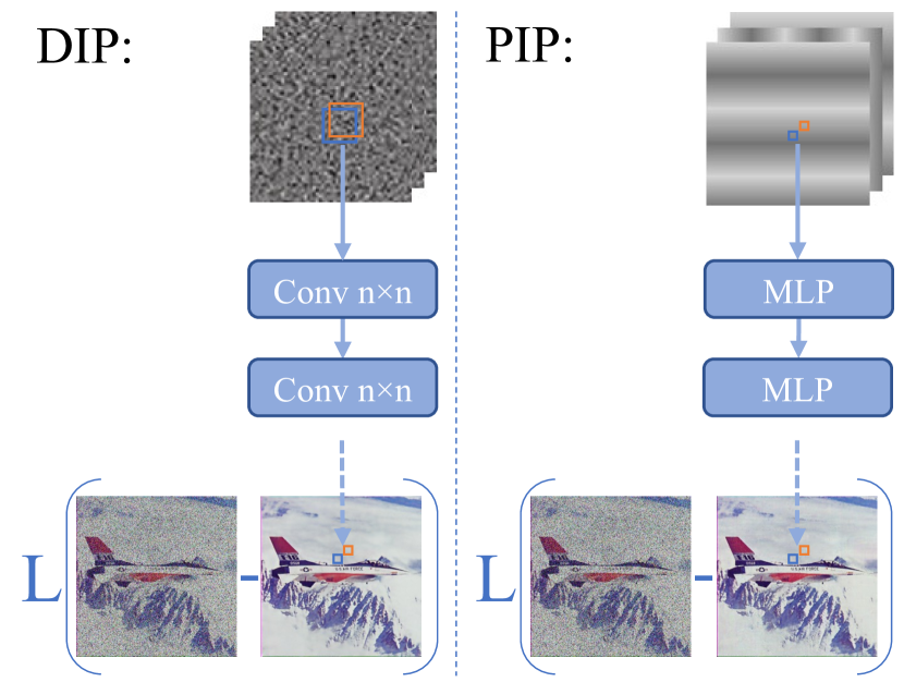
Figure 1: We offer a novel view of DIP as an implicit model that maps noise to RGB values (left). Although it maps noise to a degraded image, DIP produces a clean image. We suggest that this image prior, or regularization, stems from the fact that neighboring pixels in the output image (blue and orange in the picture) are a function of almost the same noise box in the input but a bit shifted. With this implicit model perspective, we suggest that one may achieve a similar ‘image prior’ effect by replacing the input noise with Fourier-Features. We also prove equivalence in the linear network case. As a result, we may use a simple pixel-level MLP that has much fewer parameters than the DIP CNN and still produces denoised images of the same quality. Remarkably, for video, this leads to a significant improvement.

Despite the remarkable success of DIP, it is still unclear why fitting random noise to a deteriorated image can restore the image. One explanation of how DIP works, but not why it works, is that the CNN learns to fit first the low frequencies and only later the higher frequencies, hence early stopping has a low-pass filter effect [27].

In this work, we propose that DIP should be considered as a neural implicit model that is trained to represent the target image. These models gained high popularity in the task of 3D scene representation, due to their use in Neural Radiance Fields (NeRF) [22] and its many follow-up works. They are also used for 2D image super-resolution [4], but not in the zero-shot form; they learn to map representations from a pre-trained CNN to RGB values.

Neural implicit functions are neural models trained to represent a signal, by training a multilayer perceptron (MLP) to map the coordinates of the target signal (an image in our case) to the value in these coordinates (RGB color in the case of images). This results in a neural network that implicitly represents the image. It can generate it by simply calculating the output of all its coordinates and even interpolating the image by using a finer grid as input.

Training an implicit model with the raw coordinates as input results in an oversmoothed output due to the spectral bias of neural networks towards low frequencies [25]. To overcome that, it has been shown that by mapping the input coordinates to Fourier-Features (FF), the implicit model can learn higher frequencies. This leads to a remarkable improvement in the ability of neural implicit representations.

Taking the neural implicit representation perspective, we may think of the inputs of DIP as the equivalent of the coordinate representation in implicit models. With this view in mind, DIP maps random codes to RGB values. However, despite the initial impression, this is not totally a random code. Providing independent random codes for each coordinate and then training an implicit neural model using MLP for a given image simply does not work. Yet, due to the convolutional structure of DIP, there is a “structure” in its randomness. The encoding for a specific location in the image is a shifted version of the random codes of its neighboring coordinates. Moreover, for a linear network, we prove that MLP with FF is equivalent to CNN with random inputs.” Thus, DIP can be considered as an implicit function that maps shifted random codes of the coordinates to the RGB values of the target image. With this view in mind, a natural question is why not simply use other types of positional-encodings for the input coordinates? Or more specifically, Fourier features, which have been proven to be successful for neural implicit representation.

We refer to this setup of DIP with positional-encoding inputs as “Positional-Encoding Image Prior” (PIP). In most cases, PIP-CNN outperforms DIP-CNN in image-restoration tasks such as denoising and super-resolution. Moreover, we show that using Fourier features the convolutional layers in the DIP architecture can be replaced by MLP operating independently on each coordinate (implemented by $1\times 1$ conv.). The MLP-based architecture is inspired by the MLP used for implicit models, but it is not identical as we still have skip-connection and down/up-sampling like in the original DIP. We denote this network structure as PIP-MLP, and show that it achieves similar performance compared to conventional DIP-CNN but with a lower parameter count and FLOPs. Note that using DIP-MLP fatally fails.

A remarkable advantage of PIP is that it can easily be adapted to other modalities, such as video (3D), by modifying its encoded dimensions. In contrast, extending DIP to video by employing random input encoding with 3D convolutions (3D-DIP) struggles to give reliable results. PIP, on the other hand, achieves high-quality reconstruction and significantly outperforms 3D-DIP for video tasks using a simple extension of the 2D PIP to 3D and using Fourier features that encode both spatial and temporal dimensions.

To summarize, the contributions of our paper are threefold: (i) a novel interpretation of DIP; (ii) an efficient network for self-training; and (iii) a significant improvement in video denoising and super-resolution from a single video.

2 Related Work

Positional encoding was first presented in the transformer architecture [31], where the importance of positional encoding in learning without an explicit structure was demonstrated. The visual transformer (ViT) [6] extended the transformer architecture along with the concept of positional encoding to the 2D visual domain, where an image is broken into patches and each patch contains the pixel values along with their corresponding spatial location in the image. Peiris et al. [23] used Fourier-features as the positional encoding of transformers for achieving accurate segmentation masks in medical imaging applications.

Another area of research utilizing positional encoding is implicit neural functions, which are neural networks optimized to map input coordinates to target values. It was demonstrated in [29] that representing the input coordinates as Fourier-features with a tuneable bandwidth enables a simple MLP to generate complex target domains such as images and 3D shapes while preserving their high-level details. In Neural Radiance Fields (NeRF) [22], implicit functions with Fourier features are used for synthesizing novel views of a 3D scene from sparse 2D images. SIREN [28] showed that by changing the activation function of a simple MLP to a periodic one, the network can represent the spatial and temporal derivatives so one can use a regular grid of input coordinates to successfully recover a wide range of target domains (images, videos, 3D surfaces, etc.). Local implicit image functions (LIIF) [4] represent an image as a continuous function using an implicit model. This allows it to perform super-resolution at an arbitrary scale. Xu et. al [34] show how positional encoding can be interpreted as a spatial bias in GANs. SAPE [14] and BACON [18] demonstrate how a combination of a coordinate network along with a limitation of its frequency spectrum can achieve a multi-scale representation of the target domain.

Due to the success of implicit models, coded by Fourier-features, other areas of research incorporate Fourier-features. For example, Li et al. [16] apply learned Fourier-features to control the inputs to gain better sample efficiency in many reinforcement learning problems. Bustos-Brinez et al. [2] use random Fourier-features to perform accurate data-set density estimation for anomaly detection. In this work, we treat DIP as an implicit model and show that as such it can be used with FF and an MLP.

Deep Image Prior (DIP) [30] showed that a CNN network (typically a U-net shaped architecture) can recover a clean image from a degraded image in the optimization process of mapping random noise to a degraded image. The power of DIP is shown for several key image restoration tasks such as denoising, super-resolution, and inpainting.

DIP was extended to various applications. Double-DIP [9] introduced a system composed of several DIP networks, where each learns one component of the image such that their sum is the original image. It has been used for image dehazing and foreground/background segmentation. SelfDeblur [26] performed blind image deblurring by simultaneously optimizing a DIP model and the corresponding blur kernel. In the medical imaging domain, several works tried to utilize the power of image priors to reconstruct PET images [35, 13, 10, 11]. Other works tried to improve the performance of image priors using modifications and additions to the original setup. Mataev et al. [20] and Fermanian et al. [7] combined DIP with the plug-and-play framework to improve DIP’s performance in several inverse problems. Zukerman et al. [40] showed how the back-projection fidelity term can improve DIP performance in restoration tasks like deblurring. In other areas, Kurniawan et al. [15] proposed a method for demosaicing based on DIP. Chen et al. [5] suggested DIP-based neural architecture search.

Many other works [27, 3, 32] analyzed DIP and attempted to overcome its limitations, e.g., its spectral bias and the need for early-stopping. These works, however, did so by maintaining the input as a random latent code, focusing on the limitations of the architecture itself. We challenge the use of random input for DIP and aim at improving its lack of robustness when changing the used neural architecture or the target domain, e.g., video.

Chen et al. [39] utilized DIP for large hole inpainting to remove objects from videos. Yet, naively scaling DIP to videos by replacing 2D with 3D convolutions (3D-DIP) fails to maintain temporal consistency. Thus, they introduced additional regularization and inputs to improve temporal consistency issues. Yoo et al. [36] introduced time-dependent DIP in MRI images, which encodes the temporal variations of images with a DIP network that generates MRI images. Lu et al. [19] utilize DIP for video editing and manipulation. The above works show clearly that DIP cannot be naively extended from images to video and it requires additional regularization and loss functions. On the other hand, PIP can easily be extended to videos. It learns temporal connections and preserves consistency between frames in a controllable and intuitive manner.

3 Positional-Encoding Image
Prior (PIP)

DIP [30] demonstrates that if an untrained CNN model is fitted, in a zero-shot manner, to a corrupted image, it will eventually recover the clean image without adding any explicit regularization. Formally, we have $x=f_{\theta}(z)$, where $f_{\theta}$ is a neural network that maps random input codes $z\in\mathbb{R}^{C\times W\times H}\sim U(0,\frac{1}{10})$ to image space $x\in\mathbb{R}^{3\times W\times H}$. Given a corrupted image $x_{0}$, we want to recover its clean version. Such an image reconstruction task can be formulated as an energy minimization problem

$$x^{*}=\operatornamewithlimits{argmin}_{x}E(x;x_{0})+R(x),$$ (1)

where $E(x;x_{0})$ is the data term and $R(x)$ is a regularization term. The main observation in DIP is that, due to the CNN’s image prior, the regularization term can be dropped and the data term can be optimized by adapting the model parameters with gradient descent

$$\theta^{*}=\operatornamewithlimits{argmin}_{\theta}E(f_{\theta}(z);x_{0}),\qquad x^{*}=f_{\theta^{*}}(z)\,.$$ (2)

As illustrated in Fig. 1, one may consider DIP as an implicit model and its random input as positional encoding of shifted random patches. Motivated by the above relations, in PIP, we suggest replacing the random input codes $z$ with Fourier-features as the positional-encoding of the image coordinates. These features have the advantage of being smooth, continuous, and with controllable bandwidth. For a coordinate vector $\mathbf{v}$ and set of frequencies $\{f_{0},\ldots,f_{m-1}\}$, the Fourier-features are

$$\gamma(\mathbf{v})=\left[\ldots,\cos(f_{i}\mathbf{v}),\sin(f_{i}\mathbf{v}),\ldots\right].$$ (3)

We use log-linear spaced frequencies $f_{i}=\sigma^{i/m}$, with the base $\sigma$ set by a predefined maximum frequency, such that $f_{m-1}=f_{max}$. Inspired by [17], we also tested a learnable-frequencies variant, where the frequencies are initialized as described above and then optimized together with the model parameters using gradient descent. This variant allows learning the most appropriate encoding to be used for a given image and is beneficial for some tasks.

We further suggest replacing the convolutional layers with an element-wise optimization with a coordinate-MLP, which is equivalent to performing $1\times 1$ convolution on the whole input. The intuition is that the PE image prior is sufficient to make the convolution redundant. Moreover, in the following proposition, we show that for a linear model, DIP can be formulated as learning of an implicit function with Fourier features as its input. Full details are in the appendix.

Proposition 1.

For $E$ being the $\ell_{2}$ loss and $f(z)=h*z$, where $h$ is a convolution kernel, problem (2) is equivalent to an element-wise optimization with Fourier features.

DIP uses an encoder-decoder hourglass architecture. It consists of convolutional layers with strides for down-sampling in the encoder; convolutional layers with simple bi-linear or nearest-neighbors up-sampling in the decoder; and possibly skip-connection between corresponding scales in the encoder and decoder. For PIP we adopt the same multi-scale hourglass model, but replace each convolution with $k\times k$ kernel and $s\times s$ strides with a pixel-level MLP followed by nearest-neighbor down-sampling (simply implemented as a convolution with $1\times 1$ kernel and $s\times s$ strides). Fig. 1 illustrates the modifications. The suggested architecture is more efficient in terms of compute and memory as it uses $1\times 1$ convolution instead of $3\times 3$. Also, we observe that while DIP is somewhat sensitive to the architecture used (changing $3\times 3$ kernels to $1\times 1$ makes it utterly fail), this is not the case for PIP. It is much more robust to changes and we use the same model for all tested tasks.

Finally, unlike DIP, PIP can be easily adapted to other domains. For example, when DIP is adapted to video (using 3D convolutions), additional losses have to be used to ensure temporal consistency [36]. In PIP, the model is simply adjusted by defining Fourier features for all dimensions.

Implementation details. Unless otherwise specified, we follow the original architecture choice of DIP for denoising and SR: 5 levels U-net with skip connections. Each level has 2 convolutional blocks with 128 channels, and the skip connections are with convolutional blocks with 4 channels. We also follow the original DIP hyperparameters, Adam optimizer with a learning rate of 0.01 and the same number of iterations for early-stopping. For any of the demonstrated applications, we used the original configurations and replaced only the convolutional filters from 3x3 to 1x1 and plugged in Fourier features as input instead of noise.

4 Evaluations

In this section, we first perform a quantitative evaluation of denoising and super-resolution. We also study the effect of different design choices and understand what makes PIP work from a spectral-bias perspective. We then qualitatively demonstrate the applicability of PIP to more tasks – inpainting, blind dehazing, and CLIP inversion. In addition to the examples presented in the paper, more examples for all tasks explored can be found in the appendix.

We follow the denoising and super-resolution experiments from DIP [30] using the same set of images. For denoising – 9 colored images with additive Gaussian noise ($\sigma=25$ and $\sigma=10$) and Poisson noise. For SR – the union of Set14 [38] and Set5 [1], resulting in 19 images, with $\times 4$ and $\times 8$ downscaling factors.

To demonstrate the robustness of PIP, for each task we tested 4 PIP variants, with CNN ($3\times 3$ kernels) vs. MLP ($1\times 1$ kernels) architecture and fixed vs. learned frequencies. Table 2 summarizes the results. More details appear in the appendix. We observe that fixed frequencies perform slightly better for denoising while learned frequencies perform slightly better for SR. PIP exhibits robustness to the architecture used, CNN and MLP have comparable performance, while DIP relies on the CNN and fails with MLP. Figures 2 and 3 show examples of the denoising and SR results, respectively, for both PIP and DIP. We observe a similar quality level overall, with DIP tending a little bit more to over-smoothing artifacts, and PIP to localized artifacts. We also observed that the performance on different images by DIP and PIP is highly correlated ($0.99$ correlation coef.), suggesting CNN and PE have a similar ‘prior’ effect.

We also tested PIP on 100 real-world noisy images from the PolyU dataset [33]. Results are in Table 1, additional analysis can be found in the appendix.

DnCNN	DIP	PIP
36.26dB	35.99dB	36.35dB

Table 1: Real noise performance on the PolyU dataset

			Denoising			SR
	Arch.	Freq.	$\sigma=25$	$\sigma=10$	Poisson	$\times 4$	$\times 8$
DIP	CNN	-	28.56	29.506	29.467	27.73	24.58
DIP	MLP	-	20.37	19.204	19.332	21.66	16.89
PIP	CNN	Fixed	28.80	30.011	29.957	27.867	24.03
PIP	CNN	Learned	28.28	29.795	29.813	28.09	24.26
PIP	MLP	Fixed	28.26	29.784	29.734	27.53	23.96
PIP	MLP	Learned	28.24	29.591	29.464	27.87	24.35

Table 2: Denoising and Super-Resolution evaluation. Compared to DIP-CNN, DIP-MLP fails. On the other hand, PIP is robust to the model used and does not require a CNN. Using fixed frequencies is slightly better for denoising, while learned frequencies (optimizing input frequencies together with model params) are slightly better for SR.

GT	Noisy	DIP	PIP (ours)

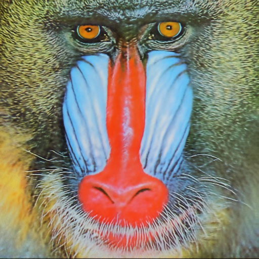
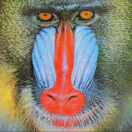
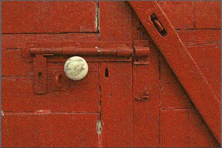
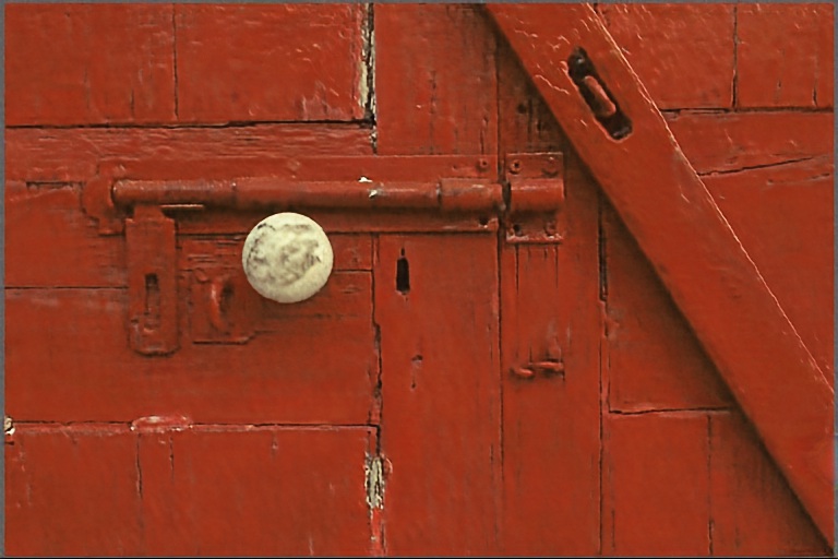
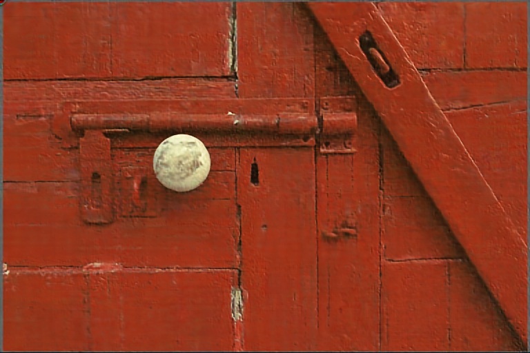
Figure 2: Image denoising examples for Gaussian noise ($\sigma=25$). From left to right: clean image (GT), noisy image, DIP (CNN) and PIP (MLP) results. The results for DIP and PIP are very similar, suggesting they follow a similar image prior.

HR	LR	DIP	PIP (ours)

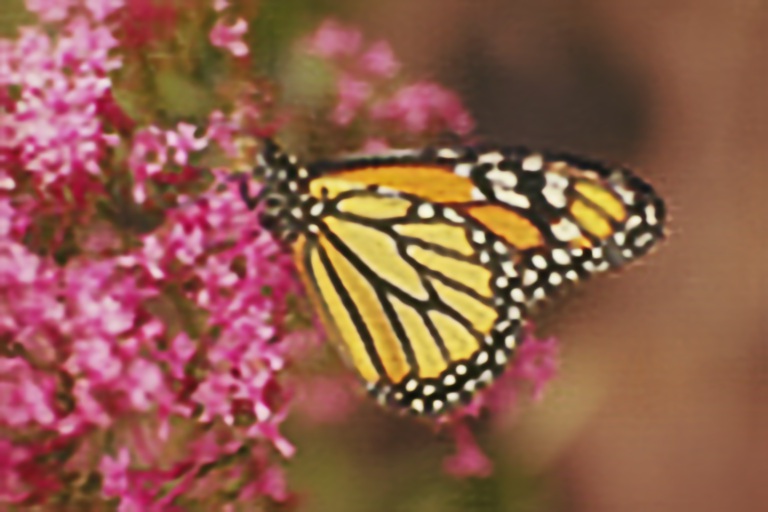
Figure 3: SR examples - The first example is for $\times 4$ SR, the second is for $\times 8$ SR. The results for DIP (CNN) and PIP (MLP) are very similar, suggesting they have a similar image prior.

U-Net vs MLP. DIP employs a U-Net architecture. It has an encoder-decoder structure, where each encoder block uses strides to downsample the image and each decoder block upsamples the image by nearest or bilinear interpolation. Parts of the original resolution signal are passed through skip connections. These down- and up-sampling operations have the effect of a low-pass filter on the parts of the signal passed through them. This can be treated as part of the image prior of the model. To test this effect we compare $1\times 1$ U-Net vs. a vanilla simple MLP applied per pixel in Table 3. It shows that for denoising, a simple MLP, commonly used in implicit models, is enough and performs just as well as the U-Net that operates in a multi-scale scheme. For SR, however, U-Net is stronger than the simple MLP. This is probably due to the fact that for this task non-local information is important for retrieving lost high frequencies. Overall, PIP, unlike DIP which requires convolutions and the U-Net structure, exhibits strong robustness to the model used. Throughout this paper, for the sake of simplicity, we use the $1\times 1$ U-Net architecture for all experiments.

Denoising DIP PIP U-Net MLP 20.37 28.26 Simple MLP 15.26 28.42

SR $\times 4$ DIP PIP U-Net MLP 21.66 27.87 Simple MLP 14.03 26.57

Table 3: The effect of the U-net structure is evaluated on both the denoising and super-resolution tasks. While DIP is ineffective without convolutions and the U-Net structure, PIP retains its performance for denoising. We observe a drop in performance for PIP on SR without the U-Net (-1.3dB), but not as significant as for DIP.

Effect of the Fourier Features (FF) frequency range. The range of input frequencies allows controlling the generated image. When $f_{max}$ in FF is too low, we generate a blurry image. When $f_{max}$ is high we can fit the high-frequency noise. However, thanks to the spectral-bias effect, early-stopping prevents fitting the noise even with high $f_{max}$.

Figure 5 demonstrates the effect of $f_{max}$. For low $f_{max}=2^{4}$ we get blurry images. We find that $2^{8}\leq f_{max}\leq 2^{10}$ provides a good balance and generates good images. But even if we use the very high $f_{max}=2^{16}$, thanks to the early stopping we still do not fit the noise despite the model capability. We also show the PSNR performance as a function of $f_{max}$ for the presented image. The performance improves till $f_{max}=2^{8}$. Then for higher frequencies the performance varies a little bit but with no clear trend of performance degradation.

A special case of limited frequency range is using a “meshgrid” input, i.e. two input channels containing the horizontal and vertical coordinates. In FF, the encoding with the lowest frequency is $\sin(x)$, which simply applies a monotonic mapping to the coordinate and hence produces a very similar representation. Note that DIP used meshgrid as input for the inpainting task and in [27] it was tested with a pure MLP. We repeat the experiment here for that task of denoising with the purpose of showing the advantage and the key role of the FF. Figure 4 compares the training of a denoising MLP model with three different options for the input: FF, meshgrid, and noise. Clearly, using noise as input with MLP layers does not work (also noted in Table 2). Observe that with meshgrid the model does not overfit and hence does not need early stopping. Yet, it is unable to reach the FF performance even after a long training. This is because it encodes only the lowest frequency, and is thus incapable of reconstructing the higher frequencies in the image. See the appendix for visual examples.

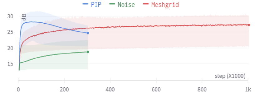
Figure 4: MLP-Denoising with FF (PIP), Meshgrid and Noise encoding. Noise encoding fails to generate a valid mapping between the input code and the target image. The meshgrid provides a much better representation but the lack of high frequencies generates an over-smoothed image. PIP lets the model produce a suitable range of frequencies such that it denoises the image well.

GT	$f_{max}=2^{4}$	$f_{max}=2^{6}$	$f_{max}=2^{8}$	$f_{max}=2^{16}$

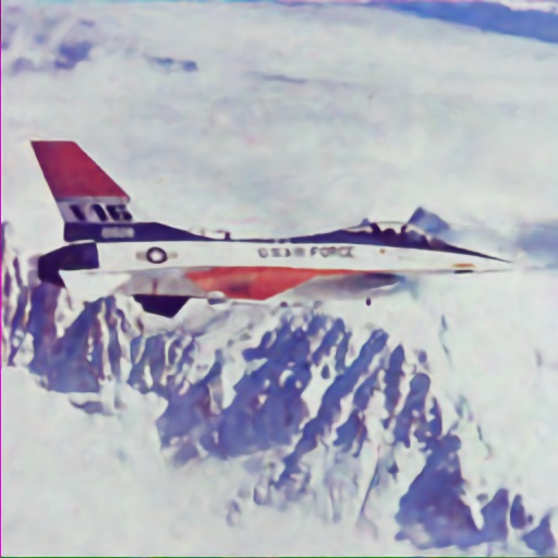
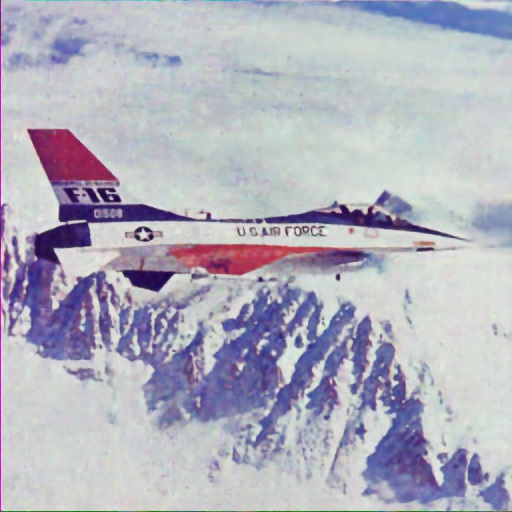
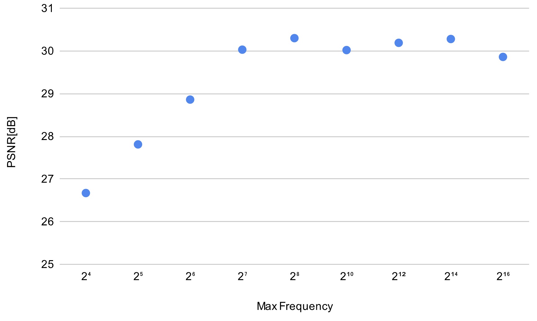
Figure 5: FF bandwidth. We compare image denoising results for various $f_{max}$. As we increase $f_{max}$ the reconstruction is sharper until it reaches a plateau around $f_{max}=2^{8}$. Using a very large frequency range, $f_{max}=2^{16}$, does not drastically affect results due to the role of early-stopping in preventing noise overfitting. On the right: PSNR as a function of $f_{max}$.

Early stopping. In our experiments, we follow the original DIP method and use a fixed number of iterations for early stopping (ES). However, there are methods for automatically choosing the stopping point. We tested EMV and WMV from [32] and found they work better for PIP compared to DIP. See quantitative results in Tab. 4.

	DIP	PIP
EMV	1.22	0.82
WMV	0.78	0.75

Table 4: Automatic early stopping difference in dB from the optimal stopping point.

Arch.	Params [M]	FLOPs [G]
DIP	2.22	65.84
PIP	0.33	12.15

Table 5: Memory and FLOPs. PIP archives similar performance to DIP with fewer params and FLOPs.

Computation efficiency. We compared the original DIP’s CNN vs. our MLP in terms of parameter count and FLOPs. Despite mostly having a similar performance, thanks to the removal of all spatial filters, the number of parameters and FLOPs decreased by a factor of $\sim 7$ and $\sim 5$; see Tab. 5.

4.1 Spectral Bias

Following [27], which analyzed DIP and showed that the model learns first the low frequencies and then the higher frequencies, we perform a similar evaluation for PIP. To test this, we fit a PIP model to a synthetic image comprised of 3 sinusoidal signals with frequencies $2\pi\cdot 4,2\pi\cdot 8,2\pi\cdot 16$, while the input frequency range is limited to $f_{max}=2\pi\cdot 8$. Figure 6 presents the synthetic image as well as the images generated during the optimization process. We also calculate the Fourier transform of the generated images and observe the rate at which the GT delta functions corresponding to the original sinusoidal signals are recovered. Clearly, the generated image fits the sinusoidals according to their frequency order, from small to large.

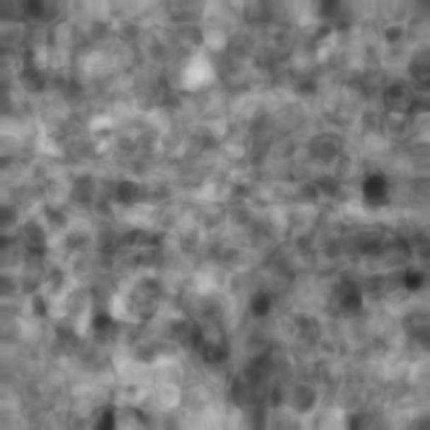
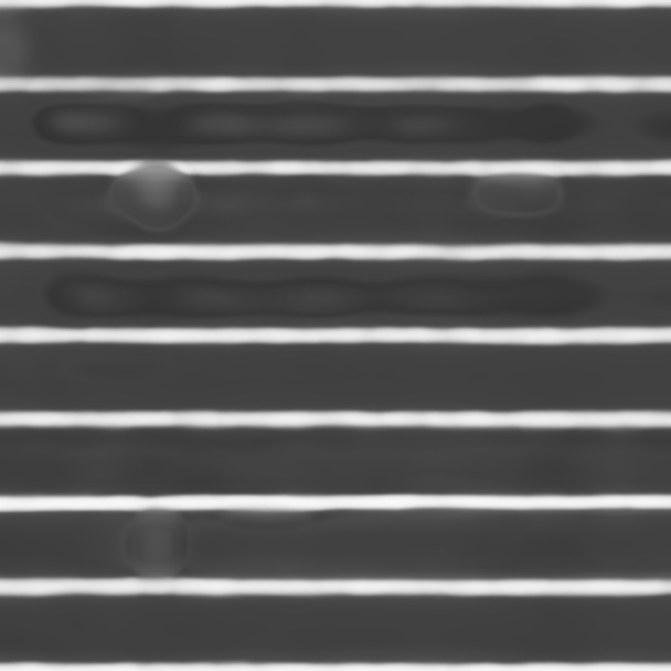
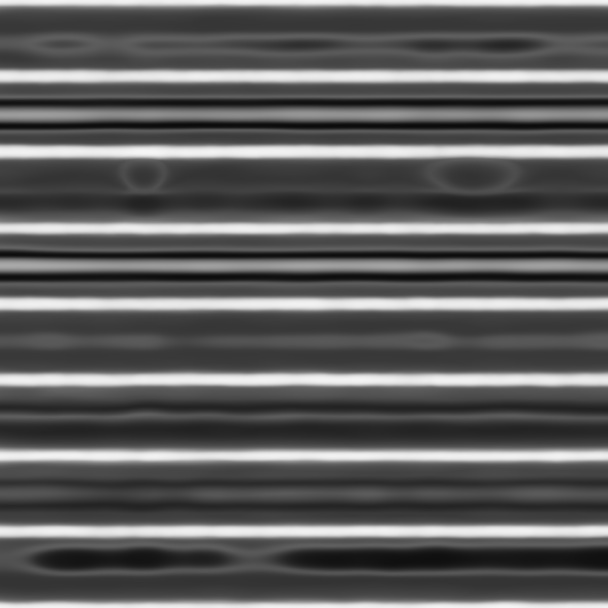
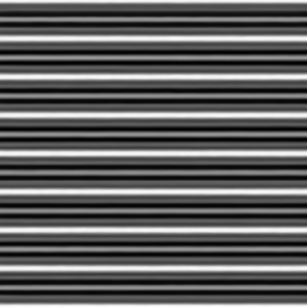
Iteration 0	Iteration 40	Iteration 80	Iteration 200	GT

Figure 6: Spectral Bias. We fit a PIP model to a synthetic image with 3 vertical frequencies (right column). We show the generated images as the training progresses (first row) and the Fourier transforms over a vertical line in the image (second row). We find that the model is biased towards first fitting the lower frequencies (lowest frequency at $\sim 40$ iterations; middle at $\sim 80$; highest at $\sim 200$). This explains why when the model is early-stopped the image’s lower frequencies are fitted while the high-frequency noise is removed. The highest frequency in the synthetic image is larger than $f_{max}$ in the model inputs, yet, the model is able to fit it too.

4.2 Additional Applications

We further demonstrate that PIP can serve as a drop-in replacement in other applications DIP is used for.

Inpainting. We follow the examples demonstrated for DIP. In both cases, we used the learned-FF configuration and increased the number of iterations to $8k$ instead of $6k$. Examples of our inpainting results are presented in Fig. 7.

Original	Masked Image	DIP	PIP-CNN	PIP-MLP

Figure 7: Image Inpainting. A comparison for large hole inpainting. PIP-CNN outperforms visually in both images, where PIP-MLP shows comparable results to DIP without any spatial kernels.

Double-PIP - Dehazing. Image dehazing is the problem of extracting a haze-free image from a hazy image. Formally, the image acquisition is modeled as $I(x)=J(x)t(x)+A(1-t)(x)$ where I is a hazy image, J is a haze-free image, A is the airlight model and $t(x)=e^{-\beta d(x)}$. In Double-DIP [9], three DIP models are trained together to generate $J(x)$ and $t(x)$ ($A$ can be derived from other algorithms or learned) with respect to the above model. Again we evaluate PIP as a drop-in replacement. We switched all noise inputs to FF and the original CNNs to our MLPs. Figure 8 shows that PIP may replace DIP also here.

Input	DIP	PIP (Ours)

Figure 8: Blind image dehazing. We compare “Double-PIP” to “Double-DIP”, where both methods produce comparable visual results.

CLIP inversion. Similarly to the original DIP inversion of AlexNet/VGG (generating images from class labels), recently DIP has been used for generating images from textual descriptions using the CLIP model [8]. DIP serves as an image generator conditioned on input text, such that the generated image embedding is close to the text embedding. Fig. 9 shows examples of image generation by inverting CLIP using both DIP and PIP. More examples are in the appendix.

DIP
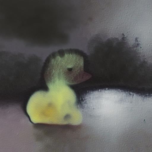
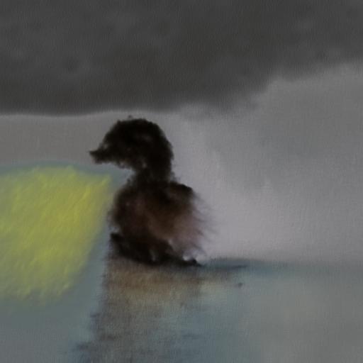
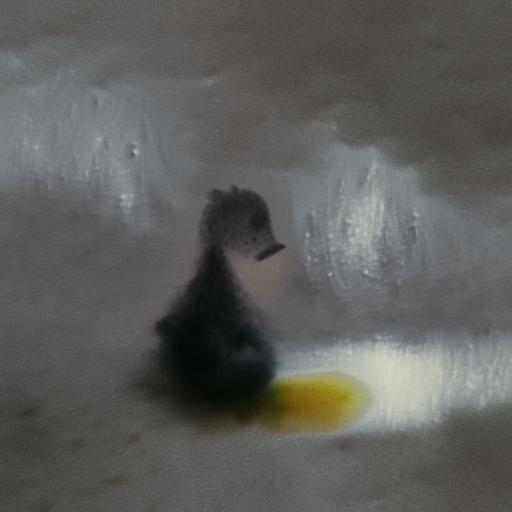
PIP

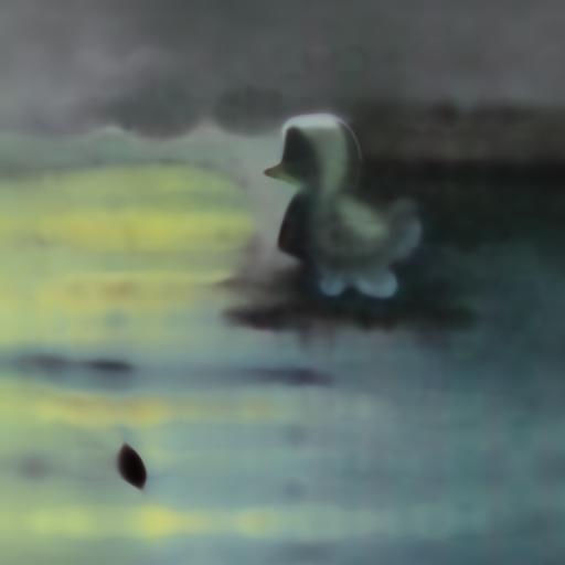
Figure 9: CLIP inversion Generated images for the description: ‘A moody painting of a lonely duckling’.

4.3 Extension to Video

	frame 12	frame 21
GT
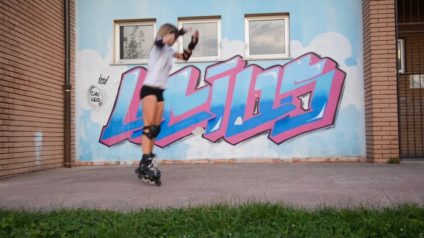
Noisy
3D-DIP
3D-PIP

Figure 10: Video denoising. We compare 3D-PIP to 3D-DIP (3D conv.). 3D-PIP generates better images (e.g. the grass area) and achieves better temporal consistency (full videos in the project page).

	Denoising			SR
Method	$\sigma=25$	$\sigma=10$	Poisson	x4
2D-DIP	26.35/0.80	26.63/0.81	26.72/0.81	25.54/0.81
3D-DIP	24.917/0.82	25.15/0.83	25.27/0.83	22.91/0.72
2D-PIP	26.17/0.80	26.61/0.81	26.67/0.81	25.45/0.78
3D-PIP	29.29/0.9	30.06/0.91	29.97/0.91	26.04/0.83

Table 6: Video-Denoising and SR: PSNR/3D-SSIM. 3D-PIP outperforms 2D-DIP (frame-by-frame) and 3D-DIP both in terms of pixel reconstruction (PSNR) and temporal consistency (3D-SSIM).

We tested an extension of PIP to video (3D-PIP) denoising and SR. To that end, we extend our positional encoding from 2D to 3D and encode the temporal domain as well as the spatial domain. Instead of stacking two spatial PEs (one for each coordinate), we stack three PEs (adding temporal encoding). Since in the case of a video, the model needs to implicitly represent a full video and not a single frame, we increase the model’s capacity. We change the model to have 6 levels instead of 5 and double the representation depth. An important observation is that other than increasing the model’s capacity, PIP does not use any 3D building blocks (such as 3D convolutional layers or tri-linear interpolation), or any additional loss and regularization as done in [4, 19].

We compare 3D-PIP to 2D-PIP (frame-by-frame) and to two versions of DIP – 2D-DIP (frame-by-frame) and 3D-DIP from [4]. We trained all video models for $5K$ iterations on all frames. We tested them on 10 videos from the DAVIS dataset [24]. Table 6 summarizes the results for all methods. In addition to PSNR, we also report SSIM-3D [37] to measure temporal consistency. 2D-DIP and 2D-PIP have comparable results. 3D-DIP is underperforming compared to 2D models. Our 3D-PIP outperforms all other models both in terms of temporal consistency and PSNR (+3dB for denoising, +0.5dB for SR). 3D-PIP achieves that with $\times 6$ fewer parameters compared to 3D-DIP. Reconstructed videos are provided in the project page.

5 Conclusions

In this paper we have shed a new light on DIP, treating it as an implicit model mapping shifted noise-blocks to RGB values. We have shown that Fourier features that are popular in implicit models can be used as a replacement for the noise inputs in DIP. Furthermore, when using PE, the convolutional layers can be replaced with MLPs, as commonly done in implicit models. We showed that the PE’s image prior is very similar to the CNN’s image prior, both in terms of quantitative performance (PSNR) and the visual appearance. Like DIP, we showed that PIP first fits the low-frequencies, providing an explanation on how it operates.

One limitation of PIP is that it uses the same amount of frequencies for all images. An adaptation to the frequencies in a given target image may improve the reconstruction significantly in some cases [14, 18]. In future work, we may explore selecting the input frequencies based on the input image content, e.g. based on BACON [18]. The frequencies can also be spatially adapted, i.e., different sets of frequencies may be employed for different regions in the image as done in SAPE [14]. For example, in the baby image in Fig. 3 it would be beneficial to use lower frequencies for the face and higher for the hat. Smartly choosing the frequencies may also help to mitigate another limitation, e.g., the need for early stopping, which is also required for DIP.

Finally, some insights from DIP and PIP might help to improve implicit models, e.g., using multi-scale processing in a U-Net architecture. The PE image prior we observed might explain the ability of NeRF to interpolate between sparse sets of input views. It can also explain the ability of NeRF to learn from noisy inputs, e.g. as exhibited by RAW-NeRF [22]. Our results hint that this ability of NeRF is not just due to averaging samples from different views but also due to the impact of PE that generates well-behaved images. Finally, we demonstrated that PIP can be used for higher dimension signals (video denoising), where DIP struggles.

Appendix

The appendix is organized as follows:
In section A we derive the full proof of Proposition 1. In section B we show to convergence of various frequencies to a synthetic image to emphasize the spectral bias. In section C we show visual examples of meshgrid inputs compared to FF-PE. In section D we show visual and quantitative results of DIP and PIP on denoising data-sets. In section E we show visual and quantitative results for Image SR for DIP and PIP. In sections F, G, and H we show visual examples for image inpainting, blind image dehazing and CLIP inversion. In sections I and J we elaborate on our video restoration tasks including visual examples.

Appendix A Proof of Proposition 1

Proposition 2.

For $E$ being the $\ell_{2}$ loss and $f(z)=h*z$, where $h$ is a convolution kernel of size $r$, problem (2) is equivalent to an element-wise optimization with Fourier features.

Proof.

We are examining the case of 1D denoising using a single linear layer without any activation. Input is as described in DIP, A uniform noise from $n\sim U[0,\frac{1}{10}]$.

The following optimization is performed:

$$\|h*n-y\|_{2}^{2},$$ (4)

where h is our spatial kernel, n is the input noise and y is the denoised image. Following [21], we can formulate the spatial convolutions into an element-wise product in the frequency domain:

$$\|\mathcal{F}^{-1}\{\mathcal{F}(h)\cdot\mathcal{F}(n)\}-y\|_{2}^{2}.$$ (5)

We will turn to focus on the left term. Denote by $F_{N}$ the $N\times N$ Discrete Fourier Transform (DFT) matrix:

$$F_{N}=\left(\begin{array}[]{ccccc}1&1&1&\ldots&1\\ 1&\omega_{N}^{1}&\omega_{N}^{2}&\ldots&\omega_{N}^{N-1}\\ 1&\omega_{N}^{2}&\omega_{N}^{4}&\ldots&\omega_{N}^{2(N-1)}\\ \vdots&\vdots&\vdots&&\vdots\\ 1&\omega_{N}^{N-1}&\omega_{N}^{2(N-1)}&\ldots&\omega_{N}^{(N-1)^{2}}\end{array}\right),$$ (6)

where,

$$\omega_{N}^{-l}=e^{-il2\pi/N}=\overline{e^{il2\pi/N}}=\overline{\omega_{N}}^{l}.$$

Thus, we may write the Fourier transformation in a matrix form as follows:

$$\widetilde{n}=\mathcal{F}(n)=\left(\begin{array}[]{ccccc}1&1&1&\ldots&1\\ 1&\omega_{N}^{1}&\omega_{N}^{2}&\ldots&\omega_{N}^{N-1}\\ 1&\omega_{N}^{2}&\omega_{N}^{4}&\ldots&\omega_{N}^{2(N-1)}\\ \vdots&\vdots&\vdots&&\vdots\\ 1&\omega_{N}^{N-1}&\omega_{N}^{2(N-1)}&\ldots&\omega_{N}^{(N-1)^{2}}\end{array}\right)\left(\begin{array}[]{c}n_{0}\\ n_{1}\\ n_{2}\\ \vdots\\ n_{N-1}\end{array}\right).$$ (7)

and similarly,

$$\widetilde{h}=\mathcal{F}(h)=\left(\begin{array}[]{ccccc}1&1&1&\ldots&1\\ 1&\omega_{N}^{1}&\omega_{N}^{2}&\ldots&\omega_{N}^{N-1}\\ 1&\omega_{N}^{2}&\omega_{N}^{4}&\ldots&\omega_{N}^{2(N-1)}\\ \vdots&\vdots&\vdots&&\vdots\\ 1&\omega_{N}^{N-1}&\omega_{N}^{2(N-1)}&\ldots&\omega_{N}^{(N-1)^{2}}\end{array}\right)\left(\begin{array}[]{c}h_{0}\\ \vdots\\ h_{r-1}\\ 0\\ \vdots\\ 0\end{array}\right).$$ (8)

Notice that since $F_{N}$ is unitary and $n$ is initialized as i.i.d. random Gaussian with zero mean, then $\tilde{n}$ is also i.i.d. random Gaussian with zero mean. Note also that $\tilde{h}$ is basically a (random) linear combination of Fourier features. Now, note that

$$\hat{y}\triangleq\mathcal{F}^{-1}(\widetilde{n}\cdot\widetilde{h})=\frac{1}{N}\left(\begin{array}[]{ccccc}1&1&1&\ldots&1\\ 1&\overline{\omega_{N}^{1}}&\overline{\omega_{N}^{2}}&\ldots&\overline{\omega_{N}^{N-1}}\\ 1&\overline{\omega_{N}^{2}}&\overline{\omega_{N}^{4}}&\ldots&\overline{\omega_{N}^{2(N-1)}}\\ \vdots&\vdots&\vdots&&\vdots\\ 1&\overline{\omega_{N}^{N-1}}&\overline{\omega_{N}^{2(N-1)}}&\ldots&\overline{\omega_{N}^{(N-1)^{2}}}\end{array}\right)\left(\begin{array}[]{c}\widetilde{h_{0}}\cdot\widetilde{n_{0}}\\ \widetilde{h_{1}}\cdot\widetilde{n_{1}}\\ \widetilde{h_{2}}\cdot\widetilde{n_{2}}\\ \vdots\\ \widetilde{h_{N-1}}\cdot\widetilde{n_{N-1}}\end{array}\right).$$ (9)

Focusing at the $k^{th}$ row, we have that

$$\hat{y}(k)=\frac{1}{N}\sum_{l=0}^{N-1}\overline{\omega_{N}^{kl}}(\widetilde{h_{l}}\cdot\widetilde{n_{l}}).$$ (10)

Since n and h are real signals, both are symmetric in the frequency domain. (namely $\widetilde{n}[k]=\widetilde{n}[N-k]$). and $\omega_{N}^{kl}$ is periodic N, we can write: (*up to N odd/even)

$$\hat{y}(k)=\frac{2}{N}(\widetilde{h_{0}}\cdot\widetilde{n_{0}})+\frac{1}{N}\sum_{l=1}^{N/2-1}(\overline{\omega_{N}^{kl}}+\overline{\omega_{N}^{-kl}})(\widetilde{h_{l}}\cdot\widetilde{n_{l}})$$ (11)

Which is equivalent to taking only the real part in the spatial domain (of a signal with a length of $\frac{N}{2}$

Using the relations between complex exponents and cosine we get the following: $\frac{2\pi}{N}\cdot m=f_{m}$ we get that we can re-write the $k^{th}$ row as follows:

$$\hat{y}(k)=\frac{2}{N}\sum_{l=1}^{N/2-1}cos(f_{l}\cdot k)\cdot(\widetilde{h_{l}}\cdot\widetilde{n_{l}})$$ (12)

From the equation, one can see that the left term in Equation (4) is equivalent to a sum of cosines that element-wise multiplied by $\hat{h_{l}}=\frac{1}{N}\widetilde{h_{l}}\cdot\widetilde{n_{l}}$. In DIP, $\widetilde{h_{l}}$ is the term that is being optimized (through the entries of $h$). In PIP, we directly optimize $\hat{h_{l}}$ and treats its entries independently.

∎

	Arch.	Freq.	Baboon	F16	House	Peppers	Lena	Kodim01	Kodim02	Kodim03	Kodim12	Avg.
DIP	CNN	-	22.00	30.12	29.56	29.79	28.89	25.67	30.19	30.62	30.20	28.56
DIP	MLP	-	13.28	15.34	13.83	14.87	13.06	16.09	20.63	15.31	14.93	15.26
PIP	CNN	Fixed	22.00	30.93	29.67	30.75	28.97	25.9	30.11	30.42	30.43	28.8
PIP	CNN	Learned	22.2	30.2	29.35	29.54	29.3	25.31	29.72	30.69	30.23	28.28
PIP	MLP	Fixed	21.52	29.92	28.47	29.77	29.12	25.27	29.59	30.41	30.48	28.26
PIP	MLP	Learned	21.58	30.02	28.69	29.8	29.35	25.13	29.78	30.25	29.52	28.24

Table 7: Detailed denoising PSNR comparison for the “standard dataset” ($\sigma=25$). Visual results can be found in Figure 13. Note that replacing random encoding with a learned one both (i) improves performance and (ii) allows replacing the CNN with MLP. PIP with MLP is more efficient and has only minor degradation in reconstruction performance, unlike DIP with MLP.

	Arch.	Freq.	Baboon	F16	House	Peppers	Lena	Kodim01	Kodim02	Kodim03	Kodim12	Avg.
DIP	CNN	-	22.207	30.906	32.568	30.786	29.726	26.122	30.936	31.415	30.537	29.467
DIP	MLP	-	16.768	18.919	20.855	18.939	17.469	18.102	23.342	20.159	19.436	19.332
PIP	CNN	Fixed	23.032	33.041	32.811	31.408	29.281	25.974	31.186	31.688	31.192	29.957
PIP	CNN	Learned	22.596	31.226	33.056	31.603	30.224	26.196	31.043	31.561	30.815	29.813
PIP	MLP	Fixed	21.945	31.97	32.789	31.276	30.006	25.886	31.028	31.165	31.539	29.734
PIP	MLP	Learned	21.998	31.805	31.682	30.828	30.374	25.527	31.1004	31.411	30.546	29.464

Table 8: Detailed denoising PSNR comparison for the “standard dataset” (Poisson). Note that replacing random encoding with a learned one both (i) improves performance and (ii) allows replacing the CNN with MLP. PIP with MLP is more efficient and has only minor degradation in reconstruction performance, unlike DIP with MLP.

	Arch.	Freq.	Baboon	F16	House	Peppers	Lena	Kodim01	Kodim02	Kodim03	Kodim12	Avg.
DIP	CNN	-	22.241	30.939	32.89	30.782	29.734	26.078	30.976	31.221	30.695	29.506
DIP	MLP	-	16.532	18.792	19.947	19.191	17.341	18.163	23.541	19.866	19.467	19.204
PIP	CNN	Fixed	22.879	31.544	32.765	31.8	30.725	26.126	31.052	32.031	31.174	30.011
PIP	CNN	Learned	22.542	32.161	32.614	31.348	30.039	26.414	31.036	30.856	31.144	29.795
PIP	MLP	Fixed	21.833	31.419	33.021	31.253	30.69	25.393	31.27	31.666	31.514	29.784
PIP	MLP	Learned	21.985	31.801	33.102	30.831	30.444	25.362	30.968	31.28	30.542	29.591

Table 9: Detailed denoising PSNR comparison for the “standard dataset” ($\sigma=10$). Note that replacing random encoding with a learned one both (i) improves performance and (ii) allows replacing the CNN with MLP. PIP with MLP is more efficient and has only minor degradation in reconstruction performance, unlike DIP with MLP.

	Arch.	Freq.	Baby	Bird	Butterfly	Head	Woman	Avg.
DIP	CNN	-	31.13	32.07	26.74	31.21	28.41	29.914
DIP	MLP	-	23.27	24.18	19.9	25.69	21.2	22.85
PIP	CNN	Fixed	32.86	32.01	25.95	31.37	28.89	30.22
PIP	CNN	Learned	32.77	32.39	26.28	31.66	28.6	30.34
PIP	MLP	Fixed	27.82	32.22	25.14	31.96	28.53	29.14
PIP	MLP	Learned	32.6	32.12	25.05	31.92	28.55	30.05

Table 10: Detailed super-resolution ($\times 4$) PSNR comparison for the Set5 dataset. Visual results can be found in Figure 15. Note that replacing random encoding with Fourier Features in PIP both (i) improves performance and (ii) allows replacing the CNN with MLP. PIP with MLP is more efficient and has only minor degradation in reconstruction performance, unlike DIP with MLP.

	Arch.	Freq.	Baboon	Barbara	Bridge	Coastguard	Comic	Face	Flowers	Foreman	Lena	Man	Monarch	Peppers	Ppt3	Zebra	Avg.
DIP	CNN	-	22.46	25.46	23.22	25.67	22.34	31.02	26.47	31.66	30.17	26.15	30.17	31.98	24.19	25.76	26.95
DIP	MLP	-	20.13	21.21	18.9	22.79	19.11	25.34	20.74	23.66	23.59	20.52	21.71	22.97	16.93	19.63	21.23
PIP	CNN	Fixed	21.64	25.5	23.5	25.64	22.25	31.87	25.63	32.13	30.92	25.82	30.86	32.57	24.07	25.98	27.03
PIP	CNN	Learned	22.53	25.59	23.62	25.25	22.33	31.91	26.59	32.29	31.41	26.48	30.48	32.7	24.68	26.1	27.78
PIP	MLP	Fixed	22.61	25.48	23.46	25.86	22.38	31.77	26.57	31.57	30.44	26.58	28.3	32.38	24.26	25.76	26.96
PIP	MLP	Learned	22.59	25.49	23.5	25.82	22.28	31.91	26.55	31.64	31.16	26.53	29.59	32.41	24.12	25.81	27.1

Table 11: Detailed super-resolution ($\times 4$) PSNR comparison for the Set14 dataset, Visual results can be found in Figures 16. Note that replacing random encoding with Fourier Features in PIP both (i) improves performance and (ii) allows replacing the CNN with MLP. PIP with MLP is more efficient and has only minor degradation in reconstruction performance, unlike DIP with MLP.

	Arch.	Freq.	Baby	Bird	Butterfly	Head	Woman	Avg.
DIP	CNN	-	28.15	27.28	20.22	29.35	24.6	25.92
DIP	MLP	-	16.82	17.82	13.74	18.96	14.64	16.4
PIP	CNN	Fixed	27.11	26.35	18.88	22.513	21.87	23.34
PIP	CNN	Learned	28.53	26.71	19.23	19.16	24.25	25.57
PIP	MLP	Fixed	28.2	25.97	18.77	28.45	23.03	24.88
PIP	MLP	Learned	28.56	26.76	19.36	29.29	24.48	25.69

Table 12: Detailed super-resolution ($\times 8$) PSNR comparison for the Set5 dataset. Visual results can be found in Figure 17. Note that replacing random encoding with FF in PIP allows replacing the CNN with MLP. PIP with MLP is more efficient and has only minor degradation in reconstruction performance, unlike DIP with MLP.

	Arch.	Freq.	Baboon	Barbara	Bridge	Coastguard	Comic	Face	Flowers	Foreman	Lena	Man	Monarch	Peppers	Ppt3	Zebra	Avg.
DIP	CNN	-	21.44	24.02	21.03	24.22	20.02	29.45	23.05	27.39	27.87	23.78	24.94	29.08	20.16	20.94	24.1
DIP	MLP	-	18.17	17.57	15.75	20.01	14.66	18.96	16.51	17.25	18.63	16.55	17.96	17.36	13.5	16.06	17.07
PIP	CNN	Fixed	21.08	23.29	20.65	24.09	19.65	29.37	22.42	28.76	27.66	21. 67	24.91	28.98	19.86	19.61	24
PIP	CNN	Learned	21.4	23.86	21.04	24.18	19.86	29.25	22.95	26.91	27.69	23.65	25.11	28.67	20.31	20.21	23.94
PIP	MLP	Fixed	21.25	23.86	20.62	23.76	19.69	28.39	22.75	26.23	27.53	23.46	24.52	28.57	19.98	20.25	23.63
PIP	MLP	Learned	21.42	23.9	21.11	24.16	19.64	29.2	22.91	27.15	27.7	23.81	24.53	28.51	20.05	20.38	23.89

Table 13: Detailed super-resolution ($\times 8$) PSNR comparison for the Set14 dataset. Visual results can be found in figure 18. Note that replacing random encoding with FF in PIP allows replacing the CNN with MLP. PIP with MLP is more efficient and has only minor degradation in reconstruction performance, unlike DIP with MLP.

Appendix B Spectral Bias

In the main paper (Section 4.1 and Figure 6), we analyzed the progression of fitting a PIP model to a synthetic image comprised of 3 sinusoidal signals with frequencies $2\pi\cdot 4,2\pi\cdot 8,2\pi\cdot 16$. We further quantify the convergence during the optimization by measuring the absolute difference between the GT and generated image Fourier transform amplitude for the 3 frequencies (see Figure 11). Clearly, lower frequencies converge faster.

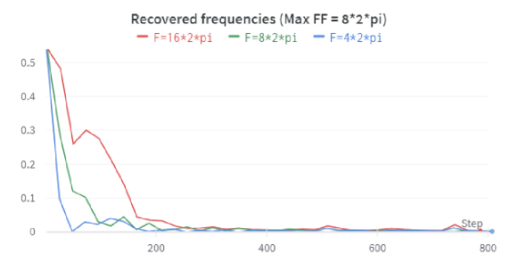
Figure 11: Spectral Bias. We measure the absolute difference between the predicted frequencies’ amplitude vs. the GT amplitudes. Lower frequencies are fitted first during the optimization.

Appendix C Comparison to meshgrid

In the main paper (Section 4 and Figure 4), we compared an MLP model with FF vs. meshgrid inputs. We showed meshgrid is unable to reach the FF performance in terms of PSNR. Here we additionally show visual results when meshgrid is used as input (Figure 12). With meshgrid as input the results are over-smoothed and the model is unable to recover details.

Org	noisy	DIP[30] (meshgrid)	PIP

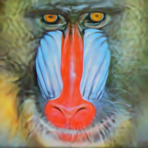
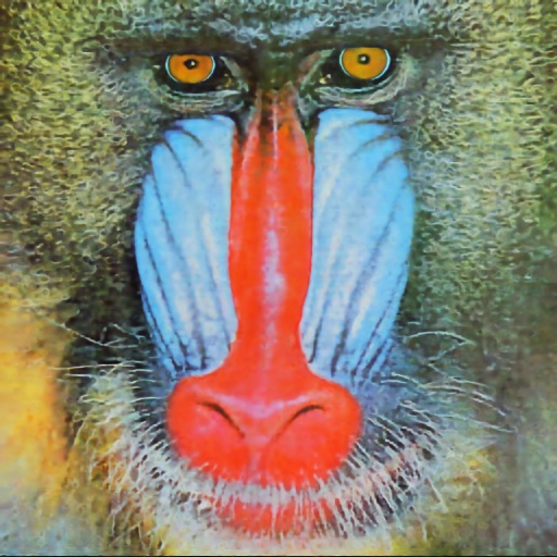
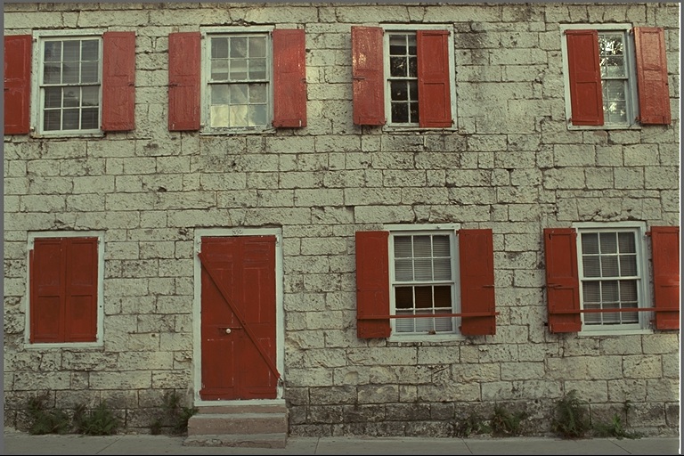
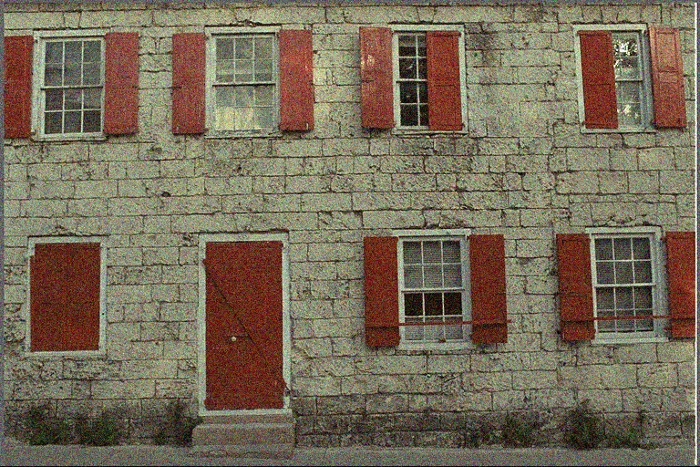
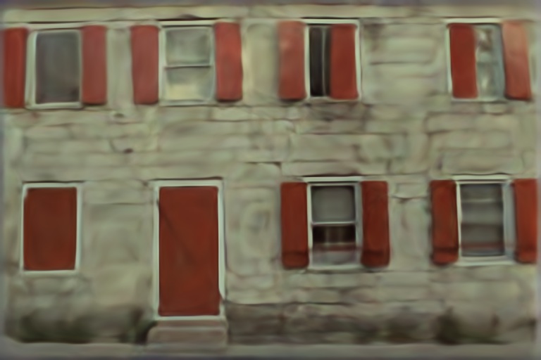
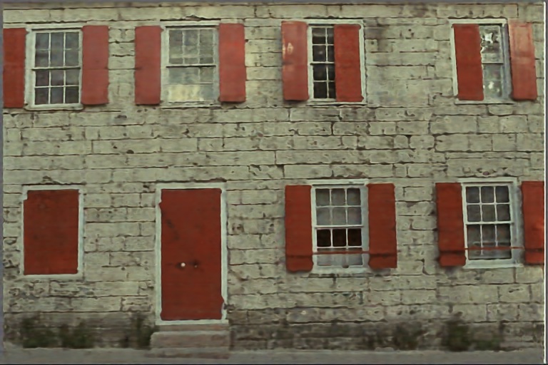
Figure 12: Image denoising ($\sigma=25$), comparison of PIP to DIP with meshgrid encoding

Appendix D Image denoising

D.1 ”Standard” Dataset

In this section, we provide a detailed PSNR comparison of all the images in the standard dataset. We provide detailed results in tables 7, 9, and 8 for Gaussian noises ($\sigma=25$, $\sigma=10$) and Poisson, respectively. Visual results of PIP-MLP vs. DIP for Gaussian ($\sigma=25$) denoising are presented in Figure 13.

Org	noisy	DIP	PIP

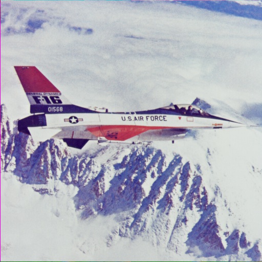
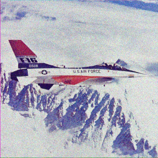
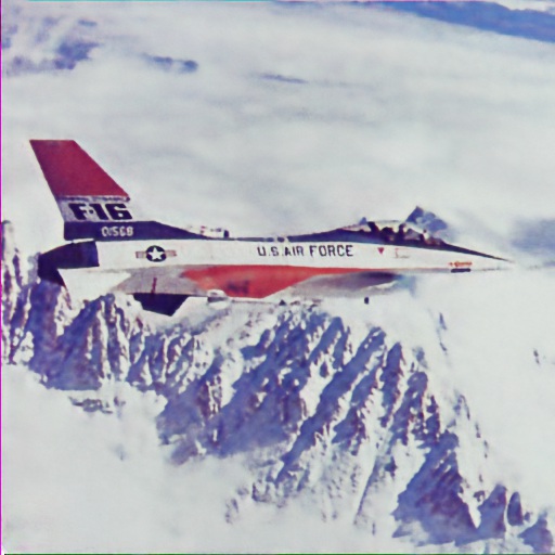
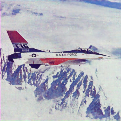
Figure 13: Image denoising ($\sigma=25$), DIP and PIP comparison - part 1. Quantitative results can be found in Table 7.

D.2 PolyU Dataset

In addition to the “standard” dataset used in the original DIP work, we also evaluated DIP and PIP on PolyU[33], a real-world noise dataset. We provide a PSNR comparison between PIP and DIP over 100 cropped images from PolyU in Table 1. Figure 14 demonstrate PIP vs. DIP performance for all 100 images - the high correlation indicates a similarity between the CNN prior and the PE prior.

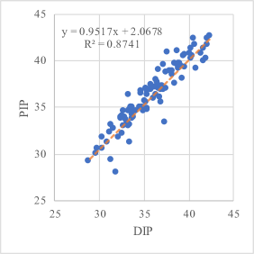
Figure 14: PIP vs. DIP PSNR performance for the 100 images of the PolyU dataset - the high correlation indicates a similarity between the CNN prior and the PE prior

Appendix E Image SR

We provide a detailed PSNR comparison between DIP and PIP along with visual examples. For PIP-CNN we changed the learning rate from 0.01 to 0.001 in both learned and fixed FF.

$\times 4$ SR

The quantitative results are presented in Table 10 (Set5) and Table 11 (Set14). The qualitative results are presented in Figure 15 (Set5) and Figure 16 (Set14).

$\times 8$ SR

The quantitative results are presented in Table 12 (Set5) and Table 13 (Set14). The qualitative results are presented in Figure 17 (Set5) and Figure 18 (Set14).

Org	LR	DIP	PIP

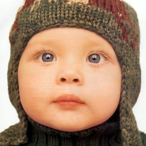
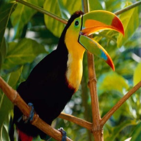
Figure 15: Image super-resolution - Set5 $\times 4$ SR, DIP vs. PIP comparison. Visual results of Table 10

Org	LR	DIP	PIP

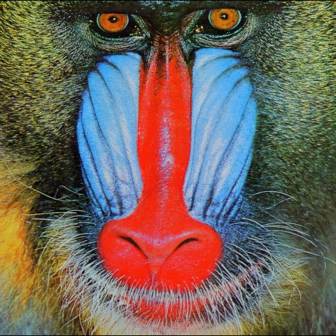
Figure 16: Image super-resolution - Set14 $\times 4$ SR, DIP vs PIP comparison. Visual results for Table 11.

Org	LR	DIP	PIP

Figure 17: Image super-resolution - Set5 $\times 8$ SR, DIP vs. PIP comparison. Visual results for Table 12.

Org	LR	DIP	PIP

Figure 18: Image super-resolution - Set14 $\times 8$ SR, DIP vs. PIP comparison. Visual results for Table 13.

Appendix F Image inpainting

We present more results of hole inpainting. We sampled images from the standard dataset (used originally for denoising) and generate for each image random holes mask. The results are presented in Figure 19. The architecture used in DIP for hole inpainting is different than the architecture used in denoising and SR in its depth (6 levels instead of 5), in its building blocks (no skip connections and bigger spatial kernels), in its embedding depth at each layer, and in the input depth (changed from 32 to 1). To make minimal adaptations to our network we simply added another layer to match the same number of levels as DIP, we keep the rest of our setup exactly as described in the paper. Since PIP is less sensitive to the architecture choice, it achieves similar or better results compared to DIP with no need for re-designing the architecture for this task.

GT	Masked image	DIP	PIP (ours)

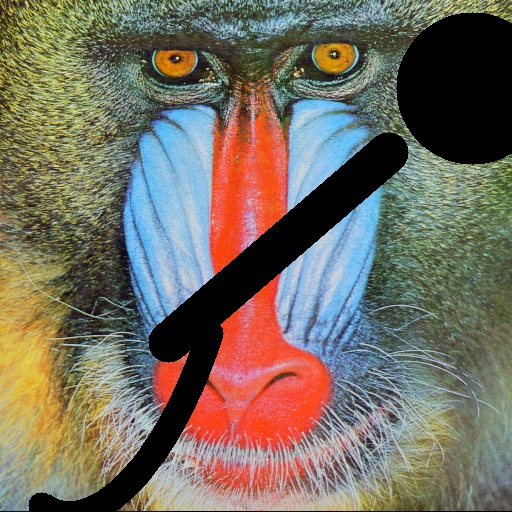
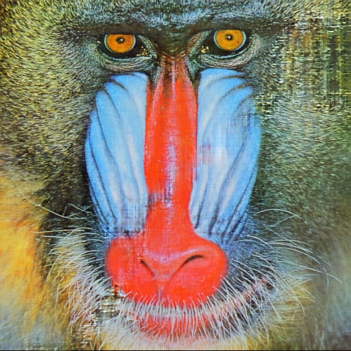
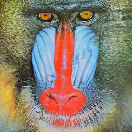
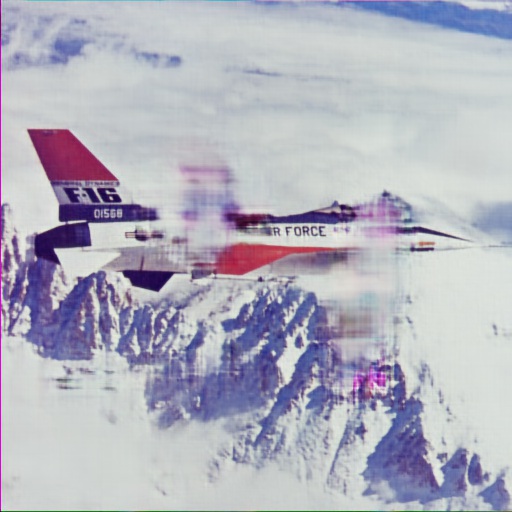
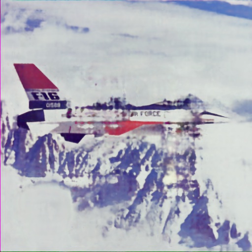
Figure 19: Image inpainting - DIP vs. PIP comparison

Appendix G Double-PIP Dehazing

We show more qualitative comparison for blind image dehazing between Double-DIP [9] and our MLP-based version, ‘Double-PIP’. We changed the input depth from 8 to 32 and switched from noise input to Fourier-features Positional-encoding. Figures 20 present Double-PIP results compared with Double-DIP (both our run of the official code and results from the paper).

Hazy	Double-DIP (official code)	Double-DIP (paper)	Double-PIP (ours)

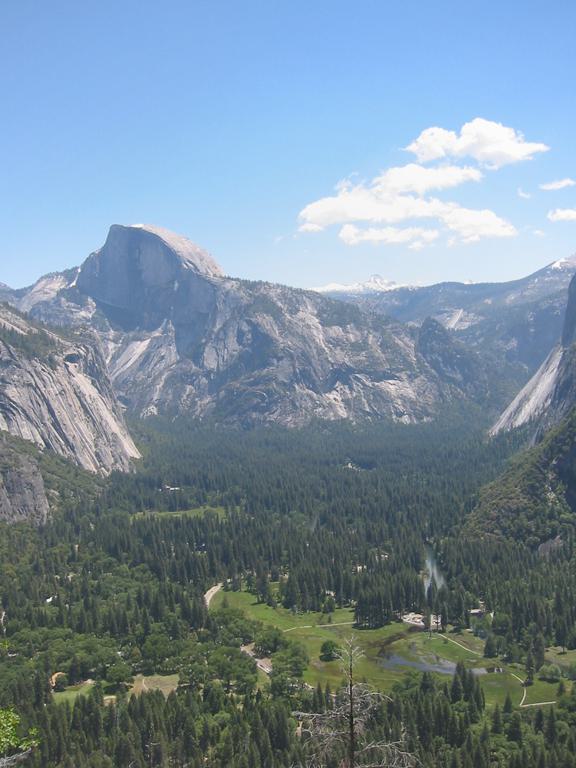
Figure 20: Blind image dehazing - Double-DIP and Double-PIP qualitative comparison

Appendix H CLIP inversion

In figures 21, 22 we provide some more examples of CLIP inversion using DIP and PIP.

DIP
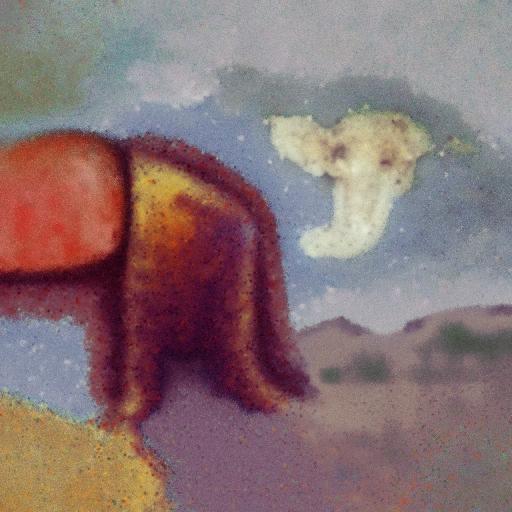
PIP

Figure 21: Generated images for the description: ‘An oil painting of an elephant sleeping in the desert’.

DIP
PIP

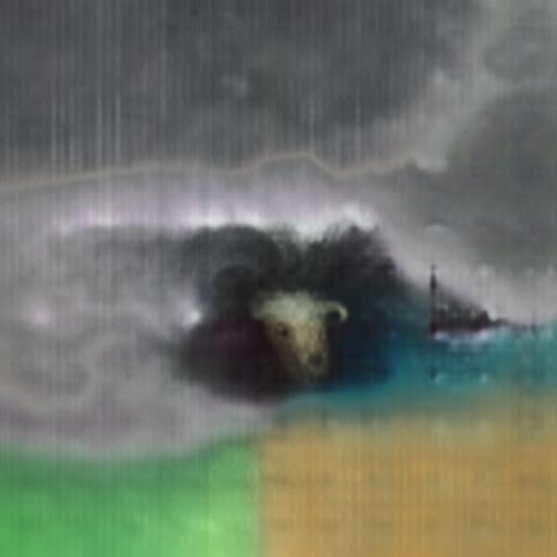
Figure 22: Generated images for the description: ‘A dark oil painting of a sheep in the middle of the sea’.

Appendix I Video Denoising

We provide a detailed table for each of the noises as described in the paper. Tables 14, 15, and 16 provide the details for Gaussian noises ($\sigma=25$, $\sigma=10$) and Poisson, respectively. 3D-PIP produces higher temporal consistency and less blurry background compared to frame-by-frame methods (2D-DIP, 2D-PIP) and 3D-DIP. Generated videos are in the project page.

	Sheep	Soccerball	Camel	Soapbox	Bear	Car turn	Bike picking	Rollerblade	Dog	Judo	Avg.
2D-DIP	23.27/0.7	23.12/0.69	24.25/0.80	27.62/0.82	24.28/0.77	27.46/0.80	26.91/0.83	28.5/0.85	26.9/0.85	31.2/0.90	26.35/0.80
3D-DIP	27.05/0.80	19.77/0.64	21.4783/0.74	26.64/0.84	24.03/0.82	26.20/0.82	23.66/0.82	25.84/0.85	22.59/0.8	31.88/0.94	24.92/0.82
2D-PIP	22.82/0.69	22.6/0.68	24.16/0.80	27.71/0.83	24.22/0.78	27.55/0.8	26.83/0.83	27.6/0.84	27.05/0.86	31.19/0.89	26.17/0.80
3D-PIP	29.61/0.93	28.11/0.90	24.44/0.81	29.94/0.89	27.81/0.90	31.09/0.91	30.08/0.93	29.05/0.89	27.45/0.87	35.27/0.97	29.29/0.90

Table 14: Gaussian ($\sigma=25$) Video Denoising - Results are PSNR[dB]/SSIM-3D. 3D-PIP outperforms frame-by-frame methods (DIP, PIP) and 3D-DIP both in terms of pixel reconstruction (PSNR) and temporal consistency (3D-SSIM)

	Sheep	Soccerball	Camel	Soapbox	Bear	Car turn	Bike picking	Rollerblade	Dog	Judo	Avg.
2D-DIP	23.62/0.71	23.47/0.69	24.56/0.81	27.88/0.83	24.50/0.77	27.61/0.8	27.05/0.82	28.83/0.87	27.33/0.87	31.43/0.91	26.63/0.81
3D-DIP	27.52/0.90	19.30/0.61	22.46/0.79	24.81/0.79	24.33/0.83	27.10/0.85	26.70/0.91	23.70/0.80	22.67/0.81	32.95/0.96	25.15/0.83
2D-PIP	23.17/0.69	22.86/0.68	24.40/0.80	28.10/0.84	24.56/0.78	27.89/0.80	27.24/0.85	28.05/0.85	27.89/0.88	32.02/0.92	26.61/0.814
3D-PIP	30.56/0.95	28.53/0.91	24.69/0.82	30.32/0.89	29.34/0.93	32.12/0.93	31.14/0.95	28.68/0.87	28.17/0.89	36.84/0.98	30.06/0.91

Table 15: Gaussian ($\sigma=10$) Video Denoising - Results are PSNR[dB]/SSIM-3D. 3D-PIP outperforms frame-by-frame methods (DIP, PIP) and 3D-DIP both in terms of pixel reconstruction (PSNR) and temporal consistency (3D-SSIM)

	Sheep	Soccerball	Camel	Soapbox	Bear	Car turn	Bike picking	Rollerblade	Dog	Judo	Avg.
2D-DIP	23.58/0.71	23.43/0.69	24.5/0.81	27.85/0.83	24.57/0.78	27.6/0.80	27.03/0.84	29.82/0.87	27.33/0.87	31.51/0.91	26.72/0.81
3D-DIP	28.4/0.92	19.5/0.62	21.52/0.75	24.56/0.79	24.44/0.83	27.66/0.88	25.82/0.89	25.25/0.84	22.67/0.81	32.92/0.96	25.27/0.83
2D-PIP	23.14/0.70	22.87/0.69	24.34/0.81	29.03/0.84	24.55/0.79	27.78/0.81	27.36/0.86	28.02/0.86	27.79/0.88	31.86/0.92	26.67/0.81
3D-PIP	30.55/0.94	27.99/0.90	25.11/0.83	30.53/0.90	28.55/0.92	31.93/0.93	30.79/0.95	30.172/0.89	28.65/0.88	35.44/0.97	29.97/0.91

Table 16: Poisson Video Denoising - Results are PSNR[dB]/SSIM-3D. 3D-PIP outperforms frame by frame methods (DIP, PIP) and 3D-DIP both in terms of pixel reconstruction (PSNR) and temporal consistency (3D-SSIM)

Appendix J Video Super-Resolution (SR)

In table 17 we provide the detailed results for video spatial super-resolution as described in the paper. In the project page We also provide the generated videos. 3D-PIP produces higher temporal consistency and less blurry background compared to frame-by-frame methods (2D-DIP, 2D-PIP) and 3D-DIP.

	Sheep	Soccerball	Camel	Soapbox	Bear	Car turn	Bike picking	Rollerblade	Dog	Judo	Avg.
2D-DIP	22.56/0.68	22.22/0.69	23.84/0.81	27.15/0.84	23.52/0.78	26.96/0.80	26.05/0.85	26.32/0.83	26.65/0.87	30.16/0.91	25.54/0.81
3D-DIP	20.43/0.58	19.8/0.57	21.71/0.72	24.05/0.75	22.46/0.71	23.82/0.71	24.04/0.8	23.17/0.74	21.04/0.72	28.54/0.89	22.91/0.72
2D-PIP	22.45/0.67	22.00/0.66	23.66/0.79	28.16/0.87	24.12/0.81	27.93/0.85	26.82/0.88	25.77/0.82	26.89/0.87	30.61/0.94	25.45/0.78
3D-PIP	22.92/0.71	23.13/0.74	23.83/0.80	28.20/0.87	24.08/0.8	27.93/0.84	26.87/0.88	26.01/0.82	26.68/0.86	30.74/0.94	26.04/0.83

Table 17: Video Super-Resolution - Results are PSNR[dB]/SSIM-3D. 3D-PIP outperforms frame-by-frame methods (DIP, PIP) and 3D-DIP both in terms of pixel reconstruction (PSNR) and temporal consistency (3D-SSIM)

References

- [1] Marco Bevilacqua, Aline Roumy, Christine Guillemot, and Marie Line Alberi-Morel. Low-complexity single-image super-resolution based on nonnegative neighbor embedding. 2012.
- [2] Oscar Bustos-Brinez, Joseph Gallego-Mejia, and Fabio A. González. Ad-dmkde: Anomaly detection through density matrices and fourier features, 2022.
- [3] Prithvijit Chakrabarty and Subhransu Maji. The spectral bias of the deep image prior. CoRR, abs/1912.08905, 2019.
- [4] Yinbo Chen, Sifei Liu, and Xiaolong Wang. Learning continuous image representation with local implicit image function. In Proceedings of the IEEE/CVF conference on computer vision and pattern recognition, pages 8628–8638, 2021.
- [5] Yun-Chun Chen, Chen Gao, Esther Robb, and Jia-Bin Huang. Nas-dip: Learning deep image prior with neural architecture search. In European Conference on Computer Vision, pages 442–459. Springer, 2020.
- [6] Alexey Dosovitskiy, Lucas Beyer, Alexander Kolesnikov, Dirk Weissenborn, Xiaohua Zhai, Thomas Unterthiner, Mostafa Dehghani, Matthias Minderer, Georg Heigold, Sylvain Gelly, et al. An image is worth 16x16 words: Transformers for image recognition at scale. arXiv preprint arXiv:2010.11929, 2020.
- [7] Rita Fermanian, Mikael Le Pendu, and Christine Guillemot. Regularizing the Deep Image Prior with a Learned Denoiser for Linear Inverse Problems. In MMSP 2021 - IEEE 23rd International Workshop on Multimedia Siganl Processing, pages 1–6, Tampere, Finland, Oct. 2021. IEEE.
- [8] Paul Fishwick. Clip inversion with dip. https://github.com/metaphorz/deep-image-prior-hqskipnet, 2021.
- [9] Yosef Gandelsman, Assaf Shocher, and Michal Irani. ” double-dip”: Unsupervised image decomposition via coupled deep-image-priors. In Proceedings of the IEEE/CVF Conference on Computer Vision and Pattern Recognition, pages 11026–11035, 2019.
- [10] Kuang Gong, Ciprian Catana, Jinyi Qi, and Quanzheng Li. Pet image reconstruction using deep image prior. IEEE Transactions on Medical Imaging, 38(7):1655–1665, 2019.
- [11] Kuang Gong, Ciprian Catana, Jinyi Qi, and Quanzheng Li. Direct reconstruction of linear parametric images from dynamic pet using nonlocal deep image prior. IEEE Transactions on Medical Imaging, 41(3):680–689, 2022.
- [12] Rana Hanocka, Gal Metzer, Raja Giryes, and Daniel Cohen-Or. Point2mesh: A self-prior for deformable meshes. ACM Trans. Graph., 39(4), 2020.
- [13] Fumio Hashimoto, Kibo Ote, and Yuya Onishi. PET image reconstruction incorporating deep image prior and a forward projection model. IEEE Transactions on Radiation and Plasma Medical Sciences, 6(8):841–846, nov 2022.
- [14] Amir Hertz, Or Perel, Raja Giryes, Olga Sorkine-Hornung, and Daniel Cohen-Or. Sape: Spatially-adaptive progressive encoding for neural optimization. Advances in Neural Information Processing Systems, 34:8820–8832, 2021.
- [15] Edwin Kurniawan, Yunjin Park, and Sukho Lee. Noise-resistant demosaicing with deep image prior network and random rgbw color filter array. Sensors, 22(5):1767, 2022.
- [16] Alexander Li and Deepak Pathak. Functional regularization for reinforcement learning via learned fourier features. Advances in Neural Information Processing Systems, 34:19046–19055, 2021.
- [17] Yang Li, Si Si, Gang Li, Cho-Jui Hsieh, and Samy Bengio. Learnable fourier features for multi-dimensional spatial positional encoding. Advances in Neural Information Processing Systems, 34:15816–15829, 2021.
- [18] David B. Lindell, Dave Van Veen, Jeong Joon Park, and Gordon Wetzstein. Bacon: Band-limited coordinate networks for multiscale scene representation. In CVPR, 2022.
- [19] Erika Lu, Forrester Cole, Tali Dekel, Andrew Zisserman, William T Freeman, and Michael Rubinstein. Omnimatte: Associating objects and their effects in video. In CVPR, 2021.
- [20] Gary Mataev, Michael Elad, and Peyman Milanfar. Deepred: Deep image prior powered by red. ArXiv, abs/1903.10176, 2019.
- [21] Michael Mathieu, Mikael Henaff, and Yann LeCun. Fast training of convolutional networks through ffts. arXiv, 2013.
- [22] Ben Mildenhall, Peter Hedman, Ricardo Martin-Brualla, Pratul P Srinivasan, and Jonathan T Barron. Nerf in the dark: High dynamic range view synthesis from noisy raw images. In Proceedings of the IEEE/CVF Conference on Computer Vision and Pattern Recognition, pages 16190–16199, 2022.
- [23] Himashi Peiris, Munawar Hayat, Zhaolin Chen, Gary Egan, and Mehrtash Harandi. A robust volumetric transformer for accurate 3d tumor segmentation. In International Conference on Medical Image Computing and Computer-Assisted Intervention, pages 162–172. Springer, 2022.
- [24] Jordi Pont-Tuset, Federico Perazzi, Sergi Caelles, Pablo Arbeláez, Alex Sorkine-Hornung, and Luc Van Gool. The 2017 davis challenge on video object segmentation. arXiv preprint arXiv:1704.00675, 2017.
- [25] Nasim Rahaman, Aristide Baratin, Devansh Arpit, Felix Draxler, Min Lin, Fred Hamprecht, Yoshua Bengio, and Aaron Courville. On the spectral bias of neural networks. In International Conference on Machine Learning, volume 97, pages 5301–5310, 2019.
- [26] Dongwei Ren, Kai Zhang, Qilong Wang, Qinghua Hu, and Wangmeng Zuo. Neural blind deconvolution using deep priors. In Proceedings of the IEEE/CVF Conference on Computer Vision and Pattern Recognition, pages 3341–3350, 2020.
- [27] Zenglin Shi, Pascal Mettes, Su bhransu Maji, and Cees G M Snoek. On measuring and controlling the spectral bias of the deep image prior. International Journal of Computer Vision, 2022.
- [28] Vincent Sitzmann, Julien N.P. Martel, Alexander W. Bergman, David B. Lindell, and Gordon Wetzstein. Implicit neural representations with periodic activation functions. In arXiv, 2020.
- [29] Matthew Tancik, Pratul P. Srinivasan, Ben Mildenhall, Sara Fridovich-Keil, Nithin Raghavan, Utkarsh Singhal, Ravi Ramamoorthi, Jonathan T. Barron, and Ren Ng. Fourier features let networks learn high frequency functions in low dimensional domains. NeurIPS, 2020.
- [30] Dmitry Ulyanov, Andrea Vedaldi, and Victor Lempitsky. Deep image prior. In Proceedings of the IEEE conference on computer vision and pattern recognition, pages 9446–9454, 2018.
- [31] Ashish Vaswani, Noam Shazeer, Niki Parmar, Jakob Uszkoreit, Llion Jones, Aidan N Gomez, Ł ukasz Kaiser, and Illia Polosukhin. Attention is all you need. In I. Guyon, U. Von Luxburg, S. Bengio, H. Wallach, R. Fergus, S. Vishwanathan, and R. Garnett, editors, Advances in Neural Information Processing Systems, volume 30. Curran Associates, Inc., 2017.
- [32] Hengkang Wang, Taihui Li, Zhong Zhuang, Tiancong Chen, Hengyue Liang, and Ju Sun. Early stopping for deep image prior, 2021.
- [33] Jun Xu, Hui Li, Zhetong Liang, David Zhang, and Lei Zhang. Real-world noisy image denoising: A new benchmark. arXiv preprint arXiv:1804.02603, 2018.
- [34] Rui Xu, Xintao Wang, Kai Chen, Bolei Zhou, and Chen Change Loy. Positional encoding as spatial inductive bias in gans, 2020.
- [35] Tatsuya Yokota, Kazuya Kawai, Muneyuki Sakata, Yuichi Kimura, and Hidekata Hontani. Dynamic pet image reconstruction using nonnegative matrix factorization incorporated with deep image prior. In Proceedings of the IEEE/CVF International Conference on Computer Vision (ICCV), October 2019.
- [36] Jaejun Yoo, Kyong Hwan Jin, Harshit Gupta, Jerome Yerly, Matthias Stuber, and Michael Unser. Time-dependent deep image prior for dynamic mri. IEEE Transactions on Medical Imaging, 2021.
- [37] Kai Zeng and Zhou Wang. 3d-ssim for video quality assessment. In 2012 19th IEEE International Conference on Image Processing, pages 621–624, 2012.
- [38] Roman Zeyde, Michael Elad, and Matan Protter. On single image scale-up using sparse-representations. In International conference on curves and surfaces, pages 711–730. Springer, 2010.
- [39] Haotian Zhang, Long Mai, Ning Xu, Zhaowen Wang, John Collomosse, and Hailin Jin. An internal learning approach to video inpainting. In Proceedings of the IEEE/CVF International Conference on Computer Vision (ICCV), October 2019.
- [40] Jenny Zukerman, Tom Tirer, and Raja Giryes. Bp-dip: A backprojection based deep image prior. In 2020 28th European Signal Processing Conference (EUSIPCO), pages 675–679. IEEE, 2021.