Analysis of Error Feedback in Federated
Non-Convex Optimization with Biased Compression

Abstract

In practical federated learning (FL) systems, e.g., wireless networks, the communication cost between the clients and the central server can often be a bottleneck. To reduce the communication cost, the paradigm of communication compression has become a popular strategy in the literature. In this paper, we focus on biased gradient compression techniques in non-convex FL problems. In the classical setting of distributed learning, the method of error feedback (EF) is a common technique to remedy the downsides of biased gradient compression. In this work, we study a compressed FL scheme equipped with error feedback, named Fed-EF. We further propose two variants: Fed-EF-SGD and Fed-EF-AMS, depending on the choice of the global model optimizer. We provide a generic theoretical analysis, which shows that directly applying biased compression in FL leads to a non-vanishing bias in the convergence rate. The proposed Fed-EF is able to match the convergence rate of the full-precision FL counterparts under data heterogeneity with a linear speedup w.r.t. the number of clients. Experiments are provided to empirically verify that Fed-EF achieves the same performance as the full-precision FL approach, at the substantially reduced communication cost.

Moreover, we develop a new analysis of the EF under partial client participation, which is an important scenario in FL. We prove that under partial participation, the convergence rate of Fed-EF exhibits an extra slow-down factor due to a so-called “stale error compensation” effect. A numerical study is conducted to justify the intuitive impact of stale error accumulation on the norm convergence of Fed-EF under partial participation. Finally, we also demonstrate that incorporating the two-way compression in Fed-EF does not change the convergence results.

In summary, our work conducts a thorough analysis of the error feedback in federated non-convex optimization. Our analysis with partial client participation also provides insights on a theoretical limitation of the error feedback mechanism, and possible directions for improvements.

1 Introduction

The general framework of federated learning (FL) has seen numerous applications in, e.g., wireless communications (e.g., 5G or 6G), Internet of Things (IoT), sensor networks, input method editor (IME), advertising, online visual object detection, public health records (Hard et al., 2018; Yang et al., 2019; Liu et al., 2020b; Rieke et al., 2020; Kairouz et al., 2021; Khan et al., 2021; Zhao et al., 2022). A centralized FL system includes multiple clients each with local data, and one central server that coordinates the training process. The goal of FL is for $n$ clients to collaboratively find a global model, parameterized by $\theta$, such that

$$\theta^{*}=\arg\min_{\theta\in\mathbb{R}^{d}}f(\theta)\mathrel{\mathop{:}}=\arg\min_{\theta\in\mathbb{R}^{d}}\frac{1}{n}\sum_{i=1}^{n}f_{i}(\theta),$$ (1)

where $f_{i}(\theta)\mathrel{\mathop{:}}=\mathbb{E}_{D\sim\mathcal{D}_{i}}\big{[}F_{i}(\theta;D)\big{]}$ is an (in general) non-convex loss function for the $i$-th client w.r.t. the local data distribution $\mathcal{D}_{i}$. In a typical FL system design, in each training round, the server first broadcasts the model to the clients. Then, each client trains the model based on the local data, after which the updated local models are transmitted back to the server and aggregated (McMahan et al., 2017; Stich, 2019; Chen et al., 2020). The number of clients, $n$, can be tens/hundreds in some applications, e.g., cross-silo FL (Marfoq et al., 2020; Huang et al., 2021) where clients are companies/organizations. In other scenarios, $n$ can be as large as millions or even billions, e.g., cross-device FL (Karimireddy et al., 2021; Khan et al., 2021), where clients can be personal/IoT devices.

There are two primary benefits from using FL: (i) the clients train the model simultaneously, which is efficient in terms of computational resources; (ii) each client’s data are kept local throughout training and are not required to be transmitted to other parties, which promotes data privacy. However, the efficiency and broad application scenarios also brings challenges for FL method design:

• Communication cost: In FL algorithms, clients are allowed to conduct multiple training steps (e.g., local SGD updates) in each round. While this has reduced the communication frequency, the one-time communication cost is still a challenge in FL systems with limited bandwidth (e.g., portable devices at the wireless network edges), which has gained growing research interest in wireless/satellite communication (Amiri and Gündüz, 2020; Niknam et al., 2020; Yang et al., 2020b, a; Khan et al., 2021; Yang et al., 2021b; Chen et al., 2022a). In particular, as modern machine learning models (e.g, deep neural networks) often contain millions or billions of model parameters, it has been an emergent task to develop efficient algorithms for transmitting the model/gradient information.

• Data heterogeneity: Unlike in the classical distributed training, the local data distribution in FL ($\mathcal{D}_{i}$ in (1)) can be different (non-iid), reflecting the typical practical scenarios where the local data held by different clients (e.g., app/website users) are highly personalized (Zhao et al., 2018; Kairouz et al., 2021; Li et al., 2022a). When multiple local training steps are taken, the local models could become “biased” towards minimizing the local losses, instead of the global loss. This phenomenon of data heterogeneity may hinder the global model to quickly converge to a good solution (Mohri et al., 2019; Li et al., 2020b; Zhao et al., 2018; Li et al., 2020a).

• Partial participation (PP): Another practical issue of FL systems is the partial participation (PP) where the clients do not join training consistently, e.g., due to unstable connection, user change or active selection (Li et al., 2020a). That is, only a fraction of clients are involved in each FL training round to update their local models and send the local update information. This may also slow down the convergence of the global model, intuitively because less data/information is used per round (Charles et al., 2021; Cho et al., 2022).

FL with compression. To overcome the main challenge of communication bottleneck, several works have analyzed FL algorithms with compressed message passing. Examples include FedPaQ (Reisizadeh et al., 2020), FedCOM (Haddadpour et al., 2021) and FedZip (Malekijoo et al., 2021). These algorithms are built upon directly compressing model updates communicated from clients to server. In particular, Reisizadeh et al. (2020); Haddadpour et al. (2021) proposed to use unbiased stochastic compressors such as stochastic quantization (Alistarh et al., 2017) and sparsification (Wangni et al., 2018), showing that with considerable communication saving, applying unbiased compression in FL could approach the performance of un-compressed FL algorithms.

Error feedback (EF) for distributed training. Besides unbiased compression, biased compressors are also commonly used in communication-efficient distributed training (Lin et al., 2018; Beznosikov et al., 2020). One simpler and popular type of compressor is the deterministic compressor, including fixed quantization (Dettmers, 2016), TopK sparsification (Aji and Heafield, 2017; Alistarh et al., 2018; Stich et al., 2018), SignSGD (Bernstein et al., 2018, 2019), etc. For these compressors, the output is a biased estimator of the true gradient. In classical distributed learning literature, it has been observed that directly updating with the biased gradients may slow down the convergence or even lead to divergence (Seide et al., 2014; Karimireddy et al., 2019; Beznosikov et al., 2020), through experiments or by counter examples. A popular remedy is the so-called error feedback (EF) strategy (Seide et al., 2014; Stich et al., 2018): in each iteration, the local worker sends a compressed gradient to the server and records the local compression error, which is subsequently used to adjust the gradient computed in next iteration, conceptually “correcting the bias” due to compression. With error feedback, using biased compression in distributed training can achieve the same convergence rate as the full-precision counterparts (Karimireddy et al., 2019; Li et al., 2022b).

Our contributions. Despite the rich literature on EF in classical distributed training settings, EF has not been well explored in the context of federated learning. In this work, we provide a thorough analysis of EF in FL. In particular, the three key features of FL: local steps, data heterogeneity and partial participation, pose challenging questions regarding the performance of EF in federated learning: (i) Can EF still achieve the same convergence rate as full-precision FL algorithms, possibly with highly non-iid local data distribution? (ii) How does partial participation change the situation and the results? In this paper, we present new algorithm and results to address these questions:

• We study Fed-EF, an FL framework with biased compression and error feedback, with two variants (Fed-EF-SGD and Fed-EF-AMS) depending on the global optimizer (SGD and adaptive AMSGrad (Reddi et al., 2018), respectively). Our investigation starts with an analysis of directly applying biased compression in FL, showing that it does not converge to zero asymptotically. Then we prove under data heterogeneity, Fed-EF has asymptotic convergence rate $\mathcal{O}(\frac{1}{\sqrt{TKn}})$ where $T$ is the number of communication rounds, $K$ is the number of local training steps and $n$ is the number of clients. Our new algorithms and analysis achieve linear speedup with respect to the number of clients, improving the previous convergence result (Basu et al., 2019) on error compensated FL (see detailed comparisons in Section 3). Moreover, Fed-EF-AMS is the first compressed adaptive FL algorithm in the literature.

• Partial participation (PP) has not been studied in the literature of distributed learning with (standard) error feedback. We initiate a new analysis of Fed-EF in this setting, by considering both local steps and non-iid data situations. We show that under PP, Fed-EF exhibits a slow-down factor of $\sqrt{n/m}$ compared with the best full-precision rate, where $m$ is the number of active clients per round. We name this as the “delayed error compensation” effect.

• Experiments are conducted to illustrate the effectiveness of the proposed methods. We show that Fed-EF matches the performance of full-precision FL with a significant reduction in communication cost, and the proposed method compares favorably with FL algorithms using unbiased compression without EF. Numerical examples are also provided to justify our theory.

2 Background and Related Work

Gradient compression in distributed optimization. In distributed SGD training systems, extensive works have applied various compression techniques to the communicated gradients. For example, the so-called “unbiased compressors” are commonly used, which include the stochastic rounding and QSGD (Alistarh et al., 2017; Zhang et al., 2017; Wu et al., 2018; Liu et al., 2020a; Xu et al., 2021), unbiased sketching (Ivkin et al., 2019; Haddadpour et al., 2020), and the magnitude based random sparsification (Wangni et al., 2018). The works (Seide et al., 2014; Bernstein et al., 2018, 2019; Karimireddy et al., 2019; Jin et al., 2020) analyzed communication compression using only the sign (1-bit) information of the gradients. Unbiased compressors can be combined with variance reduction techniques for convergence acceleration; see e.g., Gorbunov et al. (2021). On the other hand, the “biased compressors” are also popular. Common examples are the TopK compressor (Alistarh et al., 2018; Stich et al., 2018; Shi et al., 2019; Li et al., 2022b) (which only transmits gradient coordinates with largest magnitudes), fixed (or learned) quantization (Dettmers, 2016; Zhang et al., 2017; Yu et al., 2018; Malekijoo et al., 2021), and low-rank approximation (Vogels et al., 2019). See Beznosikov et al. (2020) for a summary of more biased compressors. Note that our analysis assumes a fairly general compressor which apply to a wide range of compression schemes.

Error feedback (EF). It has been shown that directly implementing biased compression in distributed SGD may lead to divergence, through empirical observations or counter examples (Seide et al., 2014; Karimireddy et al., 2019; Beznosikov et al., 2020). Error feedback (EF) are proposed to fix this issue (Seide et al., 2014; Stich et al., 2018; Karimireddy et al., 2019). In particular, with EF, distributed SGD under biased compression can match the convergence rate of the full-precision distributed SGD, e.g., also achieving linear speedup ($\mathcal{O}(1/\sqrt{Tn})$) w.r.t. the number of workers $n$ in distributed SGD (Alistarh et al., 2018; Jiang and Agrawal, 2018; Shen et al., 2018; Stich and Karimireddy, 2019; Zheng et al., 2019). Among the limited related literature on adopting EF to FL, the most relevant method is QSparse-local-SGD (Basu et al., 2019), which can be viewed as a special instance of the proposed Fed-EF-SGD variant (with fixed global learning rate). The analysis of Basu et al. (2019) did not consider data heterogeneity and partial client participation, and their convergence rate $\mathcal{O}(1/\sqrt{TK})$ does not achieve linear speedup w.r.t. the number of clients. See Section 3 and Section 4 for detailed comparisons. Recently, Richtárik et al. (2021) proposed “EF21” as an alternative to the standard EF. Fatkhullin et al. (2021) applied EF21 to FL. Our work differs from Fatkhullin et al. (2021) in that we study the standard EF (which is a different algorithm from EF21) and our theoretical analysis results exhibit a linear speedup in the number of clients.

Distributed adaptive gradient methods. Our proposed Fed-EF algorithm, in addition to SGD, also exploits AMSGrad (Reddi et al., 2018), which is an adaptive gradient method widely used in distributed and federated learning (Chen et al., 2020; Karimi et al., 2021; Reddi et al., 2021; Li et al., 2022b; Chen et al., 2022b) and industrial massive-scale CTR prediction models (Zhao et al., 2022). The core idea of adaptive gradient algorithms is to assign different implicit learning rates to different coordinates adaptively guided by the training trajectory, leading to faster convergence and less effort needed for parameter tuning. Readers are referred to the extensive literature on adaptive gradient methods, e.g., (Duchi et al., 2011; Zeiler, 2012; Kingma and Ba, 2015; Chen et al., 2019, 2020; Zhou et al., 2020; Reddi et al., 2021; Wang et al., 2021).

3 Fed-EF: Compressed Federated Learning with Error Feedback

3.1 Biased Compression Operators in Federated Learning

In this section, we introduce some existing and new deterministic compressors used in our paper which are simple and computational efficient. Throughout the paper, $[n]$ will denote the integer set $\{1,...,n\}$. $\|\cdot\|$ denotes the $l_{2}$ norm and $\|\cdot\|_{1}$ is the $l_{1}$ norm.

Definition 1 ($q_{\mathcal{C}}$-deviate compressor).

The biased $q_{\mathcal{C}}$-deviate compressor $\mathcal{C}:\mathbb{R}^{d}\mapsto\mathbb{R}^{d}$ is defined such that for $\forall x\in\mathbb{R}^{d}$, $\exists$ $0\leq q_{\mathcal{C}}<1$ s.t. $\left\|\mathcal{C}(x)-x\right\|^{2}\leq q_{\mathcal{C}}^{2}\left\|x\right\|^{2}$. In particular, two examples are Stich et al. (2018); Zheng et al. (2019):

• Let $\mathcal{S}=\{i\in[d]:|x_{i}|\geq t\}$ where $t$ is the $(1-k)$-quantile of $|x_{i}|$, $i\in[d]$. The TopK compressor with compression rate $k$ is defined as $\mathcal{C}(x)_{i}=x_{i}$, if $i\in\mathcal{S}$; $\mathcal{C}(x)_{i}=0$ otherwise.

• Divide $[d]$ into $M$ groups (e.g., neural network layers) with index sets $\mathcal{I}_{i}$, $i=1,...,M$, and $d_{i}\mathrel{\mathop{:}}=|\mathcal{I}_{i}|$. The (Grouped) Sign compressor is defined as $\mathcal{C}(x)=\big{[}\frac{\|x_{\mathcal{I}_{1}}\|_{1}}{d_{1}}sign(x_{\mathcal{I}_{1}}),...,\frac{\|x_{\mathcal{I}_{M}}\|_{1}}{d_{M}}sign(x_{\mathcal{I}_{M}})\big{]}$, with $x_{\mathcal{I}_{i}}$ the sub-vector of $x$ at indices $\mathcal{I}_{i}$.

Larger $q_{\mathcal{C}}$ indicates heavier compression, and $q_{\mathcal{C}}=0$ implies no compression, i.e. $\mathcal{C}(x)=x$. The following Proposition 3.1 is well-known, and we include the proof for clarity and completeness.

Proposition 3.1.

For the TopK compressor which selects top $k$-percent of coordinates, we have $q_{\mathcal{C}}^{2}=1-k$. For the (Group) Sign compressor, $q_{\mathcal{C}}^{2}=1-\min_{i\in[M]}\frac{1}{d_{i}}$.

Proof.

For TopK, the proof is trivial: since $\mathcal{C}(x)-x$ only contain $(1-k)d$ coordinates with lowest magnitudes, we know $\|C(x)-x\|^{2}/\|x^{2}\|\leq 1-k$.

For Sign, recall that $\mathcal{I}_{i}$ is the index set of block (group) $i$. By definition, for the $i$-th block (group) $x_{\mathcal{I}_{i}}\in\mathbb{R}^{d_{i}}$, we have

$$\|\mathcal{C}(x_{\mathcal{I}_{i}})-x_{\mathcal{I}_{i}}\|^{2} =\|x_{\mathcal{I}_{i}}-\frac{\|x_{\mathcal{I}_{i}}\|_{1}}{d_{i}}sign(x_{\mathcal{I}_{i}})\|^{2}$$

$$=\|x_{\mathcal{I}_{i}}\|^{2}+\frac{\|x_{\mathcal{I}_{i}}\|_{1}^{2}}{d_{i}^{2}}\cdot d_{i}-\frac{2\|x_{\mathcal{I}_{i}}\|_{1}^{2}}{d_{i}}$$

$$=\|x_{\mathcal{I}_{i}}\|^{2}-\|x_{\mathcal{I}_{i}}\|_{1}^{2}/d_{i}.$$

Since we have $M$ blocks, concatenating the blocks leads to

$$\|\mathcal{C}(x)-x\|^{2} =\sum_{i=1}^{M}\Big{(}\|x_{\mathcal{I}_{i}}\|^{2}-\|x_{\mathcal{I}_{i}}\|_{1}^{2}/d_{i}\Big{)}$$

$$=\|x\|^{2}-\sum_{i=1}^{M}\|x_{\mathcal{I}_{i}}\|_{1}^{2}/d_{i}$$

$$=\big{(}1-\frac{\sum_{i=1}^{M}\|x_{\mathcal{I}_{i}}\|_{1}^{2}/d_{i}}{\|x\|^{2}}\big{)}\|x\|^{2}$$

$$\leq\big{(}1-\min_{i\in[M]}\frac{\|x_{\mathcal{I}_{i}}\|_{1}^{2}}{d_{i}\|x_{\mathcal{I}_{i}}\|^{2}}\big{)}\|x\|^{2}\leq(1-\min_{i\in[M]}\frac{1}{d_{i}})\|x\|^{2},$$

where the last inequality is because $l_{1}$ norm is lower bounded by $l_{2}$ norm. ∎

Additionally, these two compression operators can be combined to derive the so-called “heavy-Sign” compressor, where we first apply TopK and then Sign, for even higher compression rate.

Definition 2 (Heavy-Sign compressor).

Let $\mathcal{C}_{k}(\cdot)$ and $\mathcal{C}_{s}(\cdot)$ be the TopK and Sign operator as in Definition 1. Then the Heavy-Sign operator is defined as $\mathcal{C}_{hv}(x)\mathrel{\mathop{:}}=\mathcal{C}_{s}\big{(}\mathcal{C}_{k}(x)\big{)}$ for $x\in\mathbb{R}^{d}$.

Proposition 3.2.

The heavy-Sign compressor satisfies Definition 1 with $q_{\mathcal{C}}^{2}=1-\min_{i\in[M]}\frac{k}{d_{i}}$.

Proof.

Recall Definition 2 that $\mathcal{C}_{k}$ denotes the TopK compressor and $\mathcal{C}_{s}$ is the Sign operator. The heavy-Sign operator $\mathcal{C}(x)=\mathcal{C}_{s}\big{(}\mathcal{C}_{k}(x)\big{)}$ admits

$$\|\mathcal{C}_{hv}(x)-x\|^{2} =\|\mathcal{C}_{s}\big{(}\mathcal{C}_{k}(x)\big{)}-\mathcal{C}_{k}(x)+\mathcal{C}_{k}(x)-x\|^{2}$$

$$=\|\mathcal{C}_{s}\big{(}\mathcal{C}_{k}(x)\big{)}-\mathcal{C}_{k}(x)\|^{2}+\|\mathcal{C}_{k}(x)-x\|^{2},$$

where the second equality holds because TopK zeros out the unpicked coordinates. By Proposition 3.1, we continue to obtain

$$\|\mathcal{C}_{hv}(x)-x\|^{2} \leq(1-\min_{i\in[M]}\frac{1}{d_{i}})\|\mathcal{C}_{k}(x)\|^{2}+\|\mathcal{C}_{k}(x)-x\|^{2}$$

$$=\|x\|^{2}-\min_{i\in[M]}\frac{1}{d_{i}}\|\mathcal{C}_{k}(x)\|^{2}\leq(1-\min_{i\in[M]}\frac{k}{d_{i}})\|x\|^{2},$$

where $M$ is the number of blocks in Sign and we use the fact that $\|\mathcal{C}_{k}(x)\|^{2}+\|\mathcal{C}_{k}(x)-x\|^{2}=\|x\|^{2}$, and $\|\mathcal{C}(x)\|\geq k\|x\|^{2}$ by Proposition 3.1. ∎

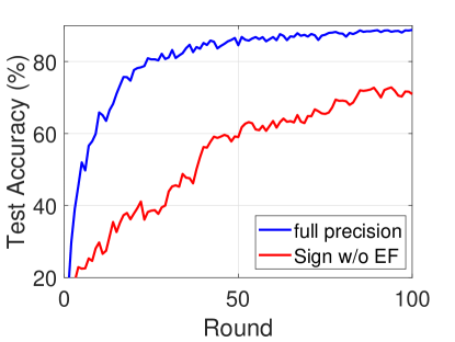
Figure 1: Test accuracy of MLP trained by Fed-SGD on MNIST dataset (LeCun et al., 1998): full-precision vs. Sign compression (Algorithm 1), $\eta=1$, $\eta_{l}=0.01$, $n=200$ non-iid clients.

Given the simplicity of the deterministic compressors, one may ask: can we directly apply biased compressors in communication-efficient FL? As an example, in Figure 1, we report the test accuracy of a multi-layer perceptron (MLP) trained on MNIST dataset in non-iid FL environment (see Section 5 for more descriptions), of Fed-SGD (Stich, 2019) with full communication (blue) versus compression using Sign (red), i.e., clients directly send compressed local model update to the server for aggregation. In Algorithm 1, we present this simple approach. We observe a catastrophic performance downgrade of using biased compression directly. In Section 3, we will demonstrate that adopting biased compression directly leads to an undesirable asymptotically non-vanishing term in the convergence rate, theoretically justifying this empirical performance degradation.

Algorithm 1 Fed-SGD with Biased Compression

1:Input: learning rates $\eta$, $\eta_{l}$

2:Initialize: central server parameter $\theta_{1}\in\mathbb{R}^{d}\subseteq\mathbb{R}^{d}$

3:for $t=1,\ldots,T$ do

4: parallel for worker $i\in[n]$ do:

5:  Receive model parameter $\theta_{t}$ from central server, set $\theta_{t,i}^{(1)}=\theta_{t}$

6:  for $k=1,\ldots,K$ do

7:   Compute stochastic gradient $g_{t,i}^{(k)}$ at $\theta_{t,i}^{(k)}$

8:   Local update $\theta_{t,i}^{(k+1)}=\theta_{t,i}^{(k)}-\eta_{l}g_{t,i}^{(k)}$

9:  end for

10:  Compute the local model update $\Delta_{t,i}=\theta_{t,i}^{(K+1)}-\theta_{t}$

11:  Send compressed model update $\widetilde{\Delta}_{t,i}=\mathcal{C}(\Delta_{t,i})$ to central server

12: end parallel

13: Central server do:

14: Global aggregation $\overline{\widetilde{\Delta}}_{t}=\frac{1}{n}\sum_{i=1}^{n}\widetilde{\Delta}_{t,i}$

15: Update the global model $\theta_{t+1}=\theta_{t}-\eta\overline{\widetilde{\Delta}}_{t}$

16:end for

Algorithm 2 Compressed Federated Learning with Error Feedback (Fed-EF)

1:Input: learning rates $\eta$, $\eta_{l}$, hyper-parameters $\beta_{1}$, $\beta_{2}$, $\epsilon$

2:Initialize: central server parameter $\theta_{1}\in\mathbb{R}^{d}\subseteq\mathbb{R}^{d}$; $e_{1,i}=\bm{0}$ the accumulator for each worker; $m_{0}=\bm{0}$, $v_{0}=\bm{0}$, $\hat{v}_{0}=\bm{0}$

3:for $t=1,\ldots,T$ do

4: parallel for worker $i\in[n]$ do:

5:  Receive model parameter $\theta_{t}$ from central server, set $\theta_{t,i}^{(1)}=\theta_{t}$

6:  for $k=1,\ldots,K$ do

7:   Compute stochastic gradient $g_{t,i}^{(k)}$ at $\theta_{t,i}^{(k)}$

8:   Local update $\theta_{t,i}^{(k+1)}=\theta_{t,i}^{(k)}-\eta_{l}g_{t,i}^{(k)}$

9:  end for

10:  Compute the local model update $\Delta_{t,i}=\theta_{t,i}^{(K+1)}-\theta_{t}$

11:  Send compressed adjusted local model update $\widetilde{\Delta}_{t,i}=\mathcal{C}(\Delta_{t,i}+e_{t,i})$ to central server

12:  Update the error $e_{t+1,i}=e_{t,i}+\Delta_{t,i}-\widetilde{\Delta}_{t,i}$

13: end parallel

14: Central server do:

15: Global aggregation $\overline{\widetilde{\Delta}}_{t}=\frac{1}{n}\sum_{i=1}^{n}\widetilde{\Delta}_{t,i}$

16: Update the global model $\theta_{t+1}=\theta_{t}-\eta\overline{\widetilde{\Delta}}_{t}$ $\triangleright$ Fed-EF-SGD

17: $m_{t}=\beta_{1}m_{t-1}+(1-\beta_{1})\overline{\widetilde{\Delta}}_{t}$ $\triangleright$ Fed-EF-AMS

18: $v_{t}=\beta_{2}v_{t-1}+(1-\beta_{2})\overline{\widetilde{\Delta}}_{t}^{2}$, $\hat{v}_{t}=\max(v_{t},\hat{v}_{t-1})$

19: Update the global model $\theta_{t+1}=\theta_{t}-\eta\frac{m_{t}}{\sqrt{\hat{v}_{t}+\epsilon}}$

20:end for

3.2 Fed-EF Algorithm

To resolve this problem, error feedback (EF), which is a popular tool in distributed training, can be adapted to federated learning. In Algorithm 2, we present the general compressed FL framework named Fed-EF, whose main steps are summarized below. In round $t$: 1) The server broadcast the global model $\theta_{t}$ to all clients (line 5); 2) The $i$-th client performs $K$ steps of local SGD updates to get local model $\theta_{t,i}^{(K)}$, compute the compressed local model update $\tilde{\Delta}_{t,i}$, updates the local error accumulator $e_{t,i}$, and sends the compressed $\tilde{\Delta}_{t,i}$ back to the server (line 6-12); 3) The server receives $\tilde{\Delta}_{t,i}$, $i\in[n]$ from all clients, takes the average, and perform a global model update using the averaged compressed local model updates (line 15-19).

Depending on the global model optimizer, we propose two variants: Fed-EF-SGD (green) which applies SGD global updates, and Fed-EF-AMS (blue), whose global optimizer is AMSGrad (Reddi et al., 2018). In Fed-EF-AMS, by the nature of adaptive gradient methods, we incorporate momentum ($m_{t}$) with different implicit dimension-wise learning rates $\eta/\hat{v}_{t}$. Additionally, for conciseness, the presented algorithm employs one-way compression (clients-to-server). In Appendix 6, we also provide a two-way compressed Fed-EF framework and demonstrate that adding the server-to-clients compression would not affect the convergence rates.

Comparison with prior work. Compared with EF approaches in the classical distributed training, e.g., Stich et al. (2018); Karimireddy et al. (2019); Zheng et al. (2019); Liu et al. (2020a); Ghosh et al. (2021); Li et al. (2022b), our algorithm allows local steps (more communication-efficiency) and uses two-side learning rates. When $\eta\equiv 1$, the Fed-EF-SGD method reduces to QSparse-local-SGD (Basu et al., 2019). In Section 4, we will demonstrate how the two-side learning rate schedule improves the convergence analysis of the one-side learning rate approach (Basu et al., 2019). On the other hand, several recent works considered compressed FL using unbiased stochastic compressors (all of which used SGD as the global optimizer). FedPaQ (Reisizadeh et al., 2020) applied stochastic quantization without error feedback to local SGD, which is improved by Haddadpour et al. (2021) using a gradient tracking trick that, however, requires communicating an extra vector from server to clients, which is less efficient than Fed-EF. Malekijoo et al. (2021) provided an empirical study on directly compressing the local updates using various compressors in Fed-SGD, while we use EF to compensate for the bias. Mitra et al. (2021) proposed FedLin, which only uses compression for synchronizing a local memory term but still requires transmitting full-precision updates. Finally, to our knowledge, Fed-EF-AMS is the first compressed adaptive FL method in literature.

4 Theoretical Results

Assumption 1 (Smoothness).

For $\forall i\in[n]$, $f_{i}$ is L-smooth: $\left\|\nabla f_{i}(x)-\nabla f_{i}(y)\right\|\leq L\left\|x-y\right\|$.

Assumption 2 (Bounded variance).

For $\forall t\in[T]$, $\forall i\in[n]$, $\forall k\in[K]$: (i) the stochastic gradient is unbiased: $\mathbb{E}\big{[}g_{t,i}^{(k)}\big{]}=\nabla f_{i}(\theta_{t,i}^{(k)})$; (ii) the local variance is bounded: $\mathbb{E}\big{[}\|g_{t,i}^{(k)}-\nabla f_{i}(\theta_{t,i}^{(k)})\|^{2}\big{]}<\sigma^{2}$; (iii) the global variance is bounded: $\frac{1}{n}\sum_{i=1}^{n}\|\nabla f_{i}(\theta_{t})-\nabla f(\theta_{t})\|^{2}\leq\sigma_{g}^{2}$.

Both assumptions are standard in the convergence analysis of stochastic gradient methods. The global variance bound $\sigma_{g}^{2}$ in Assumption 2 characterizes the difference among local objective functions, which, is mainly caused by different local data distribution $\mathcal{X}_{i}$ in (1), i.e., data heterogeneity. Following prior works on compressed FL, we also make the following additional assumption.

Assumption 3 (Compression discrepancy).

There exists some $q_{\mathcal{A}}<1$ such that $\mathbb{E}\big{[}\|\frac{1}{n}\sum_{i=1}^{n}\mathcal{C}\big{(}\Delta_{t,i}+e_{t,i}\big{)}-\frac{1}{n}\sum_{i=1}^{n}(\Delta_{t,i}+e_{t,i})\|^{2}\big{]}\leq q_{\mathcal{A}}^{2}\mathbb{E}\big{[}\|\frac{1}{n}\sum_{i=1}^{n}(\Delta_{t,i}+e_{t,i})\|^{2}\big{]}$ in every round $t\in[T]$.

In Assumption 3, if we replace “the average of compression”, $\frac{1}{n}\sum_{i=1}^{n}\mathcal{C}\big{(}\Delta_{t,i}+e_{t,i}\big{)}$, by “the compression of average”, $\mathcal{C}\big{(}\frac{1}{n}\sum_{i=1}^{n}(\Delta_{t,i}+e_{t,i})\big{)}$, the statement immediately holds by Definition 1 with $q_{\mathcal{A}}=q_{\mathcal{C}}$. Thus, Assumption 3 basically says that the above two terms stay close during training. This is a common assumption in related work on compressed distributed learning, for example, a similar assumption is used in Alistarh et al. (2018) analyzing sparsified SGD. In Haddadpour et al. (2021), for unbiased compression without EF, a similar condition is also assumed with an absolute bound. In Section C, we provide more discussion and empirical justification to validate this analytical assumption in practice.

4.1 Convergence of Directly Using Biased Compression in FL

In Figure 1, we have seen a simple example that naively transmitting the condensed local model updates by biased compressors without EF may perform poorly empirically. We now provide the theoretical convergence results on this naive strategy (Algorithm 1). More specifically, in the standard Fed-SGD algorithm (Stich, 2019), in each round $t$, after conducting $K$ local training steps to get the model update $\Delta_{t,i}$, the $i$-th client computes $\widetilde{\Delta}_{t,i}\mathrel{\mathop{:}}=\mathcal{C}(\Delta_{t,i})$ and sends it to the server. The server takes the average of the compressed gradients and updates with $\overline{\widetilde{\Delta}}_{t}=\frac{1}{n}\sum_{i=1}^{n}\widetilde{\Delta}_{t,i}$ using SGD. We have the following convergence result.

Theorem 4.1 (Fed-SGD with biased compression).

Let $\theta^{*}=\arg\min f(\theta)$, and denote $q=\max\{q_{\mathcal{C}},q_{\mathcal{A}}\}$. Consider Algorithm 1 where Fed-SGD is applied with biased communication compression. Under Assumptions 1 to 3, when $\eta_{l}\leq\frac{1}{8KL\max\{1,8(1+q^{2})\eta\}}$, we have

$$\frac{1}{T}\sum_{t=1}^{T}\mathbb{E}\big{[}\|\nabla f(\theta_{t})\|^{2}\big{]} \lesssim\frac{f(\theta_{1})-\mathbb{E}[f(\theta_{t+1})]}{\eta\eta_{l}TK}+\frac{4\eta\eta_{l}(1+q^{2})L}{n}\sigma^{2}+\frac{64q^{2}}{Kn}\sigma^{2}$$

$$+20\eta\eta_{l}^{3}(1+q^{2})K^{2}L^{3}(\sigma^{2}+6K\sigma_{g}^{2})+(320q^{2}+3)\eta_{l}^{2}KL^{2}(\sigma^{2}+6K\sigma_{g}^{2}).$$

If we choose $\eta_{l}=\Theta(\frac{1}{K\sqrt{T}})$ and $\eta=\Theta(\sqrt{Kn})$, we have

$$\frac{1}{T}\sum_{t=1}^{T}\mathbb{E}\big{[}\|\nabla f(\theta_{t})\|^{2}\big{]}=\mathcal{O}\Big{(}\frac{1+q^{2}}{\sqrt{TKn}}+\frac{1+q^{2}}{TK}(\sigma^{2}+K\sigma_{g}^{2})+\frac{q^{2}\sigma^{2}}{Kn}\Big{)}.$$ (2)

Remark 1.

When $q=0$ (no compression), the constant term in the convergence rate is erased and Theorem 4.1 recovers the $\mathcal{O}(\frac{1}{\sqrt{TKn}})$ asymptotic rate of full-precision Fed-SGD (Yang et al., 2021a).

Remark 2.

If we use unbiased compressors (e.g., stochastic quantization) instead, we can remove the constant bias term in the proof and recover the $\mathcal{O}(\frac{1}{\sqrt{TKn}})$ rate in the recent work (Haddadpour et al., 2021) for federated optimization with unbiased compression.

In Theorem 4.1, the left-hand side is the expected squared gradient norm at a uniformly chosen global model from $t=1,...,T$, which is a standard measure of convergence in non-convex optimization (i.e., “norm convergence”). In general, we see that larger $q$ (i.e., higher compression) would slow down the convergence. In the asymptotic rate (2), the first term depends on the initialization and local variance. The second term containing $\sigma_{g}^{2}$ represents the influence of data heterogeneity. The non-vanishing (as $T\rightarrow\infty$) third term is a consequence of the bias introduced by the biased compressors which decreases with smaller $q$ (i.e., less compression). This constant term (when $q\neq 0$) implies that Fed-SGD does not converge to a stationary point when biased compression is directly applied. When $q=0$ (no compression), we recover the full-precision rate as expected.

4.2 Convergence of Fed-EF: Linear Speedup Under Data Heterogeneity

We now analyze our Fed-EF algorithm which compensates the compression bias with error feedback.

Theorem 4.2 (Fed-EF-SGD).

Let $\theta^{*}=\arg\min f(\theta)$, and denote $q=\max\{q_{\mathcal{C}},q_{\mathcal{A}}\}$, $C_{1}\mathrel{\mathop{:}}=2+\frac{4q^{2}}{(1-q^{2})^{2}}$. Under Assumptions 1 to 3, when $\eta_{l}\leq\frac{1}{2KL\cdot\max\{4,\eta(C_{1}+1)\}}$, the squared gradient norm of Fed-EF-SGD iterates in Algorithm 2 can be bounded by

$$\frac{1}{T}\sum_{t=1}^{T}\mathbb{E}\big{[}\|\nabla f(\theta_{t})\|^{2}\big{]} \lesssim\frac{f(\theta_{1})-f(\theta^{*})}{\eta\eta_{l}TK}+\frac{2\eta\eta_{l}C_{1}L}{n}\sigma^{2}+10\eta\eta_{l}^{3}C_{1}K^{2}L^{3}(\sigma^{2}+6K\sigma_{g}^{2}).$$

Similar to Theorem 4.1, we may decompose the convergence rate into several parts: the first term is dependent on the initialization, the second term $\sigma^{2}$ comes from the local stochastic variance, and the last term represents the influence of data heterogeneity. We also see that larger $q$ (i.e., higher compression) slows down the convergence as expected. We will present the convergence rate under specific learning rates in Corollary 1.

In our analysis of Fed-EF-AMS, we will make the following additional assumption of bounded stochastic gradients, which is common in the convergence analysis of adaptive methods, e.g., Reddi et al. (2018); Zhou et al. (2018); Chen et al. (2019); Li et al. (2022b). Note that this assumption is only used for Fed-EF-AMS, but not for Fed-EF-SGD.

Assumption 4 (Bounded gradients).

It holds that $\|g_{t,i}^{(k)}\|\leq G$, $\forall t>0$, $\forall i\in[n]$, $\forall k\in[K]$.

We provide the convergence analysis of adaptive FL with error feedback (Fed-EF-AMS) as below.

Theorem 4.3 (Fed-EF-AMS).

With same notations as in Theorem 4.2, let $C_{1}\mathrel{\mathop{:}}=\frac{\beta_{1}}{1-\beta_{1}}+\frac{2q}{1-q^{2}}$. Under Assumptions 1 to 4, if the learning rates satisfy $\eta_{l}\leq\frac{\sqrt{\epsilon}}{8KL}\min\big{\{}\frac{1}{\sqrt{\epsilon}},\frac{2(1-q^{2})L}{(1+q^{2})^{1.5}G},\frac{1}{\max\{16,32C_{1}^{2}\}\eta},\frac{1}{3\eta^{1/3}}\big{\}}$, the Fed-EF-AMS iterates in Algorithm 2 satisfy

$$\frac{1}{T}\sum_{t=1}^{T}\mathbb{E}\big{[}\|\nabla f(\theta_{t})\|^{2}\big{]} \lesssim\frac{f(\theta_{1})-f(\theta^{*})}{\eta\eta_{l}TK}+\Big{[}\frac{5\eta_{l}^{2}KL^{2}}{2\sqrt{\epsilon}}+\frac{\eta\eta_{l}^{3}(30+20C_{1}^{2})K^{2}L^{3}}{\epsilon}\Big{]}(\sigma^{2}+6K\sigma_{g}^{2})$$

$$\hskip 36.135pt+\frac{\eta\eta_{l}L(6+4C_{1}^{2})}{n\epsilon}\sigma^{2}+\frac{(C_{1}+1)G^{2}d}{T\sqrt{\epsilon}}+\frac{3\eta\eta_{l}C_{1}^{2}LKG^{2}d}{T\epsilon}.$$

With some properly chosen learning rates, we have the following simplified results.

Corollary 1 (Fed-EF, specific learning rates).

Suppose the conditions in Theorem 4.2 and Theorem 4.3 are satisfied respectively. Choosing $\eta_{l}=\Theta(\frac{1}{K\sqrt{T}})$ and $\eta=\Theta(\sqrt{Kn})$, Fed-EF-SGD satisfies

$$\frac{1}{T}\sum_{t=1}^{T}\mathbb{E}\big{[}\|\nabla f(\theta_{t})\|^{2}\big{]}=\mathcal{O}\Big{(}\frac{f(\theta_{1})-f(\theta^{*})}{\sqrt{TKn}}+\frac{1}{\sqrt{TKn}}\sigma^{2}+\frac{\sqrt{n}}{T^{3/2}\sqrt{K}}(\sigma^{2}+K\sigma_{g}^{2})\Big{)},$$

and for Fed-EF-AMS, it holds that

$$\frac{1}{T}\sum_{t=1}^{T}\mathbb{E}\big{[}\|\nabla f(\theta_{t})\|^{2}\big{]}=\mathcal{O}\Big{(}\frac{f(\theta_{1})-f(\theta^{*})}{\sqrt{TKn}}+\frac{1}{\sqrt{TKn}}\sigma^{2}+(\frac{1}{TK}+\frac{\sqrt{n}}{T^{3/2}\sqrt{K}})(\sigma^{2}+K\sigma_{g}^{2})\Big{)}.$$

Discussion. From Corollary 1, we see that when $T\geq K$, Fed-EF-AMS and Fed-EF-SGD have the same rate of convergence asymptotically. Therefore, our following discussion applies to the general Fed-EF scheme with both variants. In Corollary 1, when $T\geq Kn\frac{\sigma_{g}^{2}}{\sigma^{2}}$, the global variance term $\sigma_{g}^{2}$ vanishes and the convergence rate becomes $\mathcal{O}(1/\sqrt{TKn})$. Thus, the proposed Fed-EF enjoys linear speedup w.r.t. the number of clients $n$, i.e., it reaches a $\delta$-stationary point (i.e., $\frac{1}{T}\sum_{t=1}^{T}\mathbb{E}\big{[}\|\nabla f(\theta_{t})\|^{2}\big{]}\leq\delta$) as long as $TK=\Theta(1/n\delta^{2})$, which matches the recent results of the full-precision counterparts (Yang et al., 2021a; Reddi et al., 2021) (Note that Reddi et al. (2021) only analyzed the special case $\beta_{1}=0$, while our analysis is more general). The condition $T\geq Kn$ to reach linear speedup considerably improves $\mathcal{O}(K^{3}n^{3})$ of the federated momentum SGD analysis in Yu et al. (2019). In terms of communication complexity, by setting $K=\Theta(1/n\delta)$, Fed-EF only requires $T=\Theta(1/\delta)$ rounds of communication to converge. This matches one of the state-of-the-art FL communication complexity results of SCAFFOLD (Karimireddy et al., 2020).

Comparison with prior results on compressed FL. As a special case of Fed-EF-SGD ($\eta\equiv 1$) and the most relevant previous work, the analysis of QSparse-local-SGD (Basu et al., 2019) did not consider data heterogeneity, and their convergence rate $\mathcal{O}(1/\sqrt{TK})$ did not achieve linear speedup either. Our new analysis improves this result, showing that EF can also match the best rate of using full communication in federated learning. For FL with direct unbiased compression (without EF), the convergence rate of FedPaQ (Reisizadeh et al., 2020) is also $\mathcal{O}(1/\sqrt{TK})$. Haddadpour et al. (2021) refined the analysis and algorithm of FedPaQ, which matches our $\mathcal{O}(1/\delta)$ communication complexity. To sum up, both Fed-EF-SGD and Fed-EF-AMS are able to achieve the convergence rates of the corresponding full-precision FL counterparts, as well as the state-of-the-art rates of federated optimization with unbiased compression.

4.3 Analysis of Fed-EF Under Partial Client Participation

Whilst being a popular strategy in classical distributed training, error feedback has not been analyzed under partial participation (PP), which is an important feature of FL. Next, we provide new analysis and results of EF under this setting, considering both local steps and data heterogeneity in federated learning. In each round $t$, assume only $m$ randomly chosen clients (without replacement) indexed by $\mathcal{M}_{t}\subseteq[n]$ are active and participate in training (i.e., changing $i\in[n]$ to $i\in\mathcal{M}_{t}$ at line 4 of Algorithm 2). For the remaining $(n-m)$ inactive clients, we simply set $e_{t,i}=e_{t-1,i}$, $\forall i\in[n]\setminus\mathcal{M}_{t}$. The convergence rate is given as below.

Theorem 4.4 (Fed-EF, partial participation).

In each round, suppose $m$ randomly chosen clients in $\mathcal{M}_{t}$ participate in the training. Under Assumptions 1 to 3, suppose the learning rates satisfy $\eta_{l}\leq\min\Big{\{}\frac{1}{6},\frac{m}{96C^{\prime}\eta},\frac{m^{2}}{53760(n-m)C_{1}\eta},\frac{1}{4\eta},\frac{1}{32C_{1}\eta}\Big{\}}\frac{1}{KL}$. Fed-EF-SGD admits

$$\frac{1}{T}\sum_{t=1}^{T}\mathbb{E}\big{[}\|\nabla f(\theta_{t})\|^{2}\big{]}\lesssim\frac{f(\theta_{1})-f(\theta^{*})}{\eta\eta_{l}TK}+\Big{[}\frac{\eta\eta_{l}L}{m}+\frac{8\eta\eta_{l}C_{1}Ln}{m^{2}}\Big{]}\sigma^{2}+\frac{3\eta\eta_{l}C^{\prime}KL}{m}\sigma_{g}^{2}$$

$$\hskip 86.72377pt+\Big{[}\frac{5\eta_{l}^{2}KL^{2}}{2}+\frac{15\eta\eta_{l}^{3}C^{\prime}K^{2}L^{3}}{m}+\frac{560\eta\eta_{l}C_{1}(n-m)L}{m^{2}}\Big{]}(\sigma^{2}+6K\sigma_{g}^{2}),$$

where $C_{1}=\frac{q^{2}}{(1-q^{2})^{3}}$ and $C^{\prime}=\frac{n-m}{n-1}$. Choosing $\eta=\Theta(\sqrt{Km})$, $\eta_{l}=\Theta(\frac{\sqrt{m}}{K\sqrt{Tn}})$, we have

$$\frac{1}{T}\sum_{t=1}^{T}\mathbb{E}\big{[}\|\nabla f(\theta_{t})\|^{2}\big{]} =\mathcal{O}\Big{(}\frac{\sqrt{n}}{\sqrt{m}}\big{(}\frac{f(\theta_{1})-f(\theta^{*})}{\sqrt{TKm}}+\frac{1}{\sqrt{TKm}}\sigma^{2}+\frac{\sqrt{K}}{\sqrt{Tm}}\sigma_{g}^{2}\big{)}\Big{)}.$$

Remark 3.

We present Fed-EF-SGD for simplicity. With more complicated analysis, similar result applies to Fed-EF-AMS yielding the same asymptotic convergence rate as Fed-EF-SGD.

Remark 4.

When $m=n$ (full participation), Theorem 4.4 reduces to the $\mathcal{O}(1/\sqrt{TKn})$ rate in Corollary 1. When $q=0$ (no compression), we can recover the $\mathcal{O}(\sqrt{K/Tm})$ rate of full-precision Fed-SGD under PP (Yang et al., 2021a).

The convergence rate in Theorem 4.4 involves $m$ in the denominator, instead of $n$ as in Corollary 1, which is a result of larger gradient estimation variance due to client sampling. Importantly, compared with the $\mathcal{O}(\sqrt{K/Tm})$ rate of Yang et al. (2021a) for full-precision local SGD under partial participation, Theorem 4.4 extracts an additional slow-down factor of $\sqrt{n/m}$.

Effect of delayed error compensation. We argue that this is a consequence of the mechanism of error feedback. Intuitively, with full participation where each client is active in every round, EF itself can, to a large extent, be regarded as subtly “delaying” the “untransmitted” gradient information ($\mathcal{C}(\Delta_{t})-\Delta_{t}$) to the next iteration. However, under partial participation, in each round $t$, the error accumulator of a chosen client actually contains the latest information from round $t-s$, where $s$ can be viewed as the “lag” which follows a geometric distribution with $\mathbb{E}[s]=n/m$. In some sense, this shares similar spirit to the problem of asynchronous distributed optimization with delayed gradients (e.g., Agarwal and Duchi (2011); Lian et al. (2015)). The delayed error information in Fed-EF under PP is likely to pull the model away from heading towards a stationary point (i.e., slower down the norm convergence), especially for highly non-convex loss functions. In Section 5, we will propose a simple strategy to empirically justify (and to an extent mitigate) the negative impact of the stale error compensation on the norm convergence.

5 Numerical Study

We provide numerical results to show the empirical efficacy of Fed-EF in communication-efficient FL problems and justify our theoretical analysis. Our main objective is to show: 1) Fed-EF is able to provide matching performance as full-precision FL, with significantly less communication; 2) the stale error compensation effect would indeed slower down the norm convergence of Fed-EF under partial participation. We include representative main results here and place the implementation details and more figures and tables in Appendix B.

5.1 Experiment Setup

Datasets. We present experiments on three popular FL datasets. The MNIST dataset (LeCun et al., 1998) contains 60000 training examples and 10000 test samples of $28\times 28$ gray-scale hand-written digits from 0 to 9. The FMNIST dataset (Xiao et al., 2017) has the same input size and train/test split as MNIST, but the samples are fashion products (e.g., clothes and bags). The CIFAR-10 (Krizhevsky, 2009) dataset includes 50000 natural images of size $32\times 32$ each with 3 RGB channels for training and 10000 images for testing. There are 10 classes, e.g., airplanes, cars, cats, etc. We follow a standard strategy for CIFAR-10 dataset to pre-process the training images by a random crop, a random horizontal flip and a normalization of the pixel values to have zero mean and unit variance. For test images, we only apply the normalization step.

Federated setting. In our experiments, we test $n=200$ clients. The clients’ local data are set to be highly non-iid (heterogeneous), where we restrict the local data samples of each client to come from at most two classes: we first split the data samples into $2n=400$ shards each containing samples from only one class; then each client is assigned with two shards uniformly at random. We run $T=100$ rounds, where one FL training round is finished after all the clients have performed one epoch of local training. The local mini-batch size is $32$, which means that the clients conduct 10 local iterations per round. Regarding partial participation, we uniformly randomly sample $m$ clients in each round. We present the results at multiple sampling proportion $p=m/n$ (e.g., $p=0.1$ means choosing $20$ active clients per round). To measure the communication cost, we report the accumulated number of bits transmitted from the client to server (averaged over all clients), assuming that full-precision gradients are $32$-bit encoded.

Methods and compressors. For both Fed-EF variants, we implement Sign compressor, and TopK compressor with compression rate $k\in\{0.001,0.01,0.05\}$. We also employ a more compressive strategy heavy-Sign (Definition 2) where Sign is applied after TopK (i.e., a further $32$x compression over TopK under same sparsity). We test heavy-Sign with $k\in\{0.01,0.05,0.1\}$. We compare our method with the analogue federated learning approaches using full-precision updates and using unbiased stochastic quantization “Stoc” without error feedback (Alistarh et al., 2017) without error feedback. For this compressor, we test parameter $b\in\{1,2,4\}$. For SGD, this algorithm is equivalent to FedCOM/FedPaQ (Reisizadeh et al., 2020; Haddadpour et al., 2021). The detailed introduction of the competing methods (with both SGD and AMSGrad variants) can be found in Algorithm 4 in Appendix A. In our experiments, the reported results are averaged over multiple independent runs.

5.2 Fed-EF Matches Full-Precision FL with Substantially Less Communication

Firstly, we demonstrate the feasible performance of Fed-EF in practical FL tasks. For both datasets, we train a ReLU activated CNN with two convolutional layers followed by one max-pooling, one dropout and two fully-connected layers before the softmax output. We test each compression strategy with different compression ratios, and report the test accuracy in Figure 2 and Figure 3 for MNIST and FMNIST, respectively, when the participation rate $p=0.5$. The set of results when $p=0.1$ is placed in Appendix B. We see that in general, the performance gets worse when we increase the compression rate, as expected from the theory.

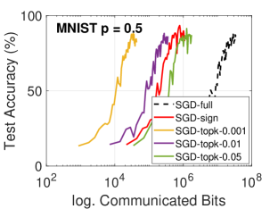
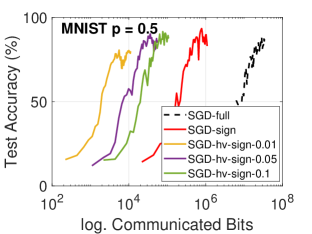
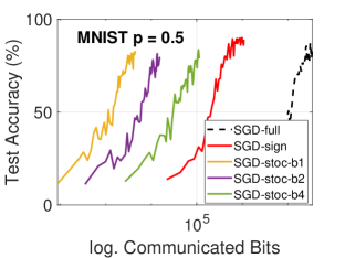
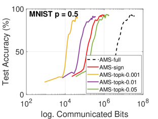
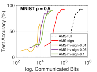
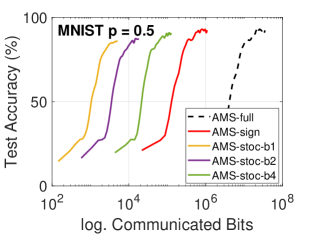
Figure 2: Test accuracy of Fed-EF on MNIST dataset trained by CNN. “sign”, “topk” and “hv-sign” are applied with Fed-EF, while “Stoc” is the stochastic quantization without EF. Participation rate $p=0.5$, non-iid data. 1st row: Fed-EF-SGD. 2nd row: Fed-EF-AMS.

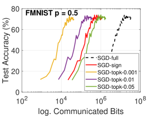
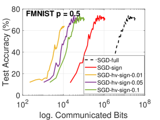
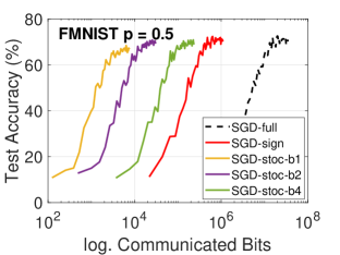
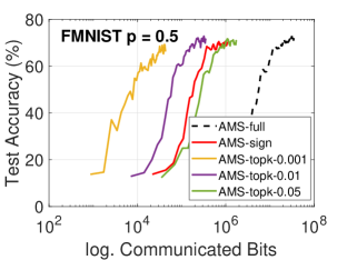
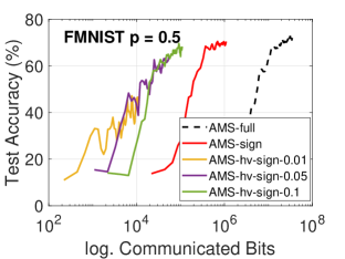
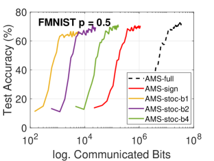
Figure 3: Test accuracy of Fed-EF on FMNIST dataset trained by CNN. “sign”, “topk” and “hv-sign” are applied with Fed-EF, while “Stoc” is the stochastic quantization without EF. Participation rate $p=0.5$, non-iid data. 1st row: Fed-EF-SGD. 2nd row: Fed-EF-AMS.

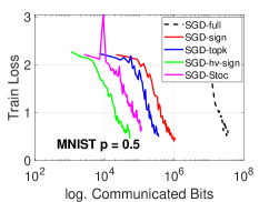
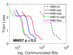
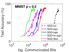
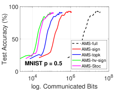
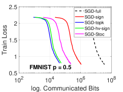
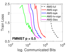
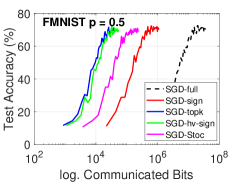
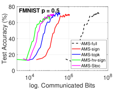
Figure 4: Training loss and test accuracy v.s. communicated bits on MNIST and FMNIST datasets, participation rate $p=0.5$. “sign”, “topk” and “hv-sign” are applied with Fed-EF, while “Stoc” is the stochastic quantization without EF.

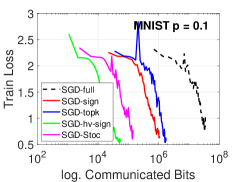
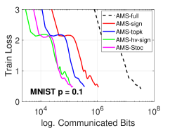
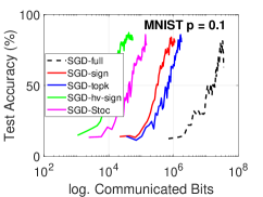
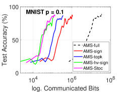
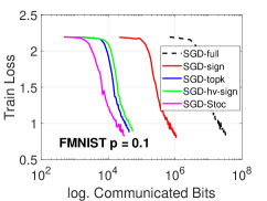
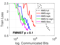
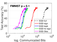
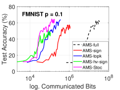
Figure 5: Training loss and test accuracy v.s. communicated bits on MNIST and FMNIST datasets, participation rate $p=0.1$. “sign”, “topk” and “hv-sign” are applied with Fed-EF, while “Stoc” is the stochastic quantization without EF.

To make a more straightforward comparison, in Figure 4 ($p=0.5$) and Figure 5 ($p=0.1$), we present the training loss and test accuracy curves (respective compression ratios) chosen by the following rule: for each method, we present the curve with highest compression level that achieves the best full-precision test accuracy (within $0.1\%$); if the method does not match the full-precision performance, we present the curve with the highest test accuracy. The exact test accuracy and standard deviations can be found in Appendix B. We observe the following:

• The proposed Fed-EF (including both variants) is able to achieve the same performance as the full-precision methods with substantial communication reduction, e.g., heavy-Sign and TopK reduce the communication by more than 100x without losing accuracy. Sign also provides 30x compression with matching accuracy as full-precision training.

• In Figure 4, on MNIST, the test accuracy of Stoc (stochastic quantization without EF) is slightly lower than Fed-EF-SGD with heavy-Sign, yet requiring more communication.

• With more aggressive $p=0.1$ (Figure 5), Fed-EF with a proper compressor still performs on a par with full-precision algorithms. While Sign performs well on MNIST, we notice that fixed sign-based compressors (Sign and heavy-Sign) are outperformed by TopK for Fed-EF-AMS on FMNIST. We conjecture that this is because with small participation rate, sign-based compressors tend to assign a same implicit learning rate across coordinates (controlled by the second moment $\hat{v}$), making adaptive method less effective. In contrast,magnitude-preserving compressors (e.g., TopK and Stoc) may better exploit the adaptivity of AMSGrad.

5.3 Results on CIFAR-10 and ResNet

We present additional experiments to illustrate that Fed-EF is able to match the full-precision training on larger models, on the task of CIFAR-10 image classification. For this experiment, we train a ResNet-18 (He et al., 2016) network for 200 rounds. The clients local data are distributed in the same way as described above which is highly non-iid.

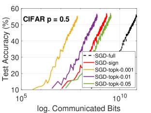
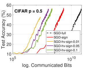
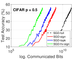
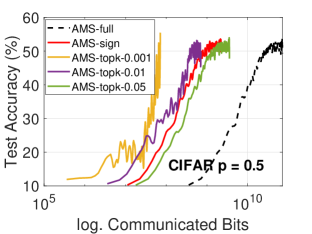
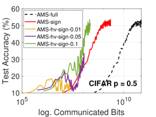
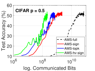
Figure 6: CIFAR-10 dataset trained by ResNet-18. Test accuracy of Fed-EF with TopK, Sign and heavy-Sign compressors. Participation rate $p=0.5$, non-iid data. 1st row: Fed-EF-SGD. 2nd row: Fed-EF-AMS. The last column presents the corresponding curves that achieve the full-precision accuracy using lowest communication.

In Figure 6, we plot the test accuracy of Fed-EF with different compressors. Again, we see that Fed-EF (both variants) is able to attain the same accuracy level as the corresponding full-precision federated learning algorithms. For Fed-EF-SGD, the compression rate is around 32x for Sign, 100x for TopK and $\sim$300x for heavy-Sign. For Fed-EF-AMS, the compression ratio can also be around hundreds. Note that for Fed-EF-AMS, the training curve of TopK-0.001 is not stable. Though it reaches a high accuracy, we still plot TopK-0.01 in the third column for comparison.

In Figure 7 we report the results for partial participation with $p=0.1$. Similarly, for SGD, all three compressors are able to match the full-precision accuracy, with significantly reduced number of communicated bits. For Fed-EF-AMS, similar to the observations on FMNIST, we see that TopK outperforms Sign and heavy-Sign, and achieve the performance of full-precision method with 100x compression ratio. Sign also performs reasonably well.

In conclusion, our results on CIFAR-10 and ResNet again confirm that compared with standard full-precision FL algorithms, the proposed Fed-EF scheme can provide significant communication reduction without empirical performance drop in test accuracy, under both data heterogeneity and partial client participation.

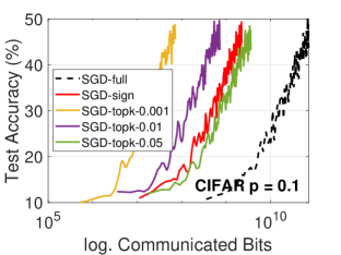
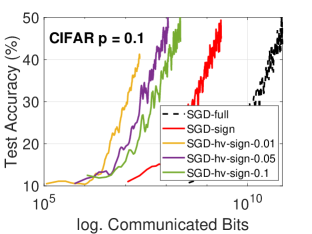
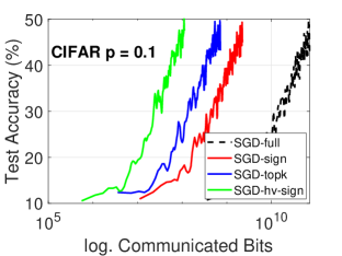
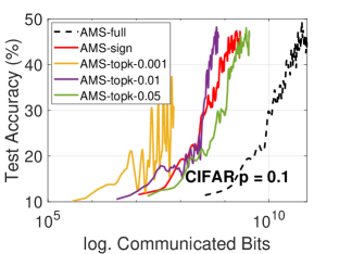
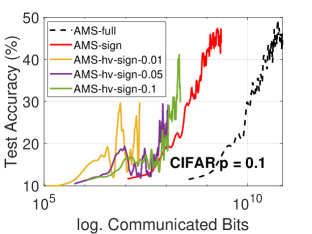
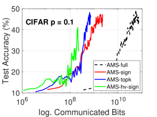
Figure 7: CIFAR-10 dataset trained by ResNet-18. Test accuracy of Fed-EF with TopK, Sign and heavy-Sign compressors. Participation rate $p=0.1$, non-iid data. 1st row: Fed-EF-SGD. 2nd row: Fed-EF-AMS. The last column presents the corresponding curves that achieve the full-precision accuracy using lowest communication.

5.4 Analysis of Norm Convergence and Delayed Error Compensation

We empirically evaluate the norm convergence to verify the theoretical speedup properties of Fed-EF and the effect of delayed error compensation in partial participation (PP). Recall that from Theorem 1, in full participation case, reaching a $\delta$-stationary point requires running $\Theta(1/n\delta^{2})$ rounds of Fed-EF (i.e., linear speedup). From Theorem 4.4, when $n$ is fixed, our result implies that the speedup should be super-linear against $m$, the number of participating clients, due to the additional stale error effect. In other words, altering $m$ under PP is expected to have more impact on the convergence than altering $n$ with full participation.

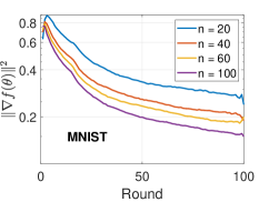
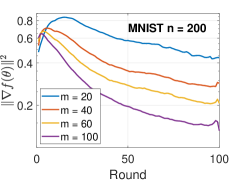
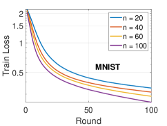
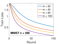
Figure 8: MLP on MNIST with TopK-0.01 compressed Fed-EF: Squared gradient norm (left two) and train loss (right two) against the number of training rounds, averaged over 20 independent runs.

We train an MLP (which is also used for Figure 1) with one hidden layer of 200 neurons. In Figure 8, we report the squared gradient norm and the training loss on MNIST under the same non-iid FL setting as above (the results on FMNIST are similar). In the full participation case, we implement Fed-EF-SGD with $n=20,40,60,100$ clients; for the partial participation case, we fix $n=200$ and alter $m=20,40,60,100$. According to our theory, we set $\eta=0.1\sqrt{n}$ (or $0.1\sqrt{m}$) and $\eta_{l}=0.1$. We see that: 1) In general, the convergence of Fed-EF is faster with increasing $n$ or $m$, which confirms the speedup property; 2) The gaps among curves in the PP setting (the 2nd and 4th plot) is larger than those in the full-participation case (the 1st and 3rd plot), which suggests that the acceleration brought by increasing $m$ under PP is more significant than that of increasing $n$ in full-participation by a same proportion, which is consistent with our theoretical implications.

Error restarting. To further embody the intuitive impact of delayed error compensation under PP, we test a simple strategy called “error restarting” as follows: for each client $i$ in round $t$, if the error accumulator was last updated more than $S$ (a threshold) rounds ago (i.e., before round $t-S$), we simply restart its error accumulator by setting $e_{t,i}=0$, which effectively eliminates the error information that is “too old”.

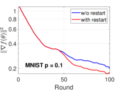
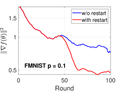
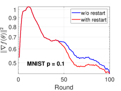
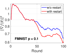
Figure 9: Squared gradient norm of Fed-EF (TopK-0.01) under PP with error restarting, $S=10$. Left two panels: logistic regression. Right two panels: MLP. $n=200$, $\eta=1$, $\eta_{l}=0.1$.

In Figure 9, we first run Fed-EF for 50 rounds, and then apply error restarting with threshold $S=10$. As we see, after prohibiting heavily delayed error information, the gradient norm is smaller than that of continuing running standard Fed-EF, i.e., the model finds a stationary point faster. These results illustrate the influence of stale error compensation in Fed-EF, and that properly handling this staleness might be a promising direction for theoretical improvement in the future.

Remark 5.

Note that the error restarting trick is a simple heuristic to illustrate the impact of delayed error compensation in Fed-EF. If we consider theoretical convergence rates, this strategy may not bring improvement since zeroing out the error accumulators, although reducing the stale errors, also leads to biased compression when it is triggered. Therefore, as shown by Theorem 4.1, it would result in an additional non-vanishing bias term in the convergence rate, worse than Theorem 4.4 asymptotically. In fact, this strategy plays a trade-off between the staleness in error feedback and biased compression, which could be beneficial empirically if properly balanced.

6 Two-Way Compression in Fed-EF

Algorithm 3 Fed-EF Scheme with Two-Way Compression

1:Input: learning rates $\eta$, $\eta_{l}$, hyper-parameters $\beta_{1}$, $\beta_{2}$, $\epsilon$

2:Initialize: central server parameter $\theta_{1}\in\mathbb{R}^{d}\subseteq\mathbb{R}^{d}$; $e_{1,i}=\bm{0}$ the accumulator for each worker; $m_{0}=\bm{0}$, $v_{0}=\bm{0}$, $\hat{v}_{0}=\bm{0}$; $\phi_{1}=\tilde{H}_{t}=\bm{0}$; $\theta_{0,i}^{(1)}=\theta_{1}$ for all $i\in[n]$

3:for $t=1,\ldots,T$ do

4: parallel for worker $i\in[n]$ do:

5:  Receive $\tilde{H}_{t}$ from the server and set $\theta_{t,i}^{(1)}=\theta_{t-1,i}^{(1)}+\tilde{H}_{t}$ $\triangleright$ Download compression

6:  for $k=1,\ldots,K$ do

7:   Compute stochastic gradient $g_{t,i}^{(k)}$ at $\theta_{t,i}^{(k)}$

8:   Local update $\theta_{t,i}^{(k+1)}=\theta_{t,i}^{(k)}-\eta_{l}g_{t,i}^{(k)}$

9:  end for

10:  Compute the local model update $\Delta_{t,i}=\theta_{t,i}^{(K+1)}-\theta_{t}$

11:  Send compressed adjusted local update $\widetilde{\Delta}_{t,i}=\mathcal{C}(\Delta_{t,i}+e_{t,i})$ to central server

12:  Update the error $e_{t+1,i}=e_{t,i}+\Delta_{t,i}-\widetilde{\Delta}_{t,i}$

13: end parallel

14: Central server do:

15: Global aggregation $\overline{\widetilde{\Delta}}_{t}=\frac{1}{n}\sum_{i=1}^{n}\widetilde{\Delta}_{t,i}$

16:  Compress $\tilde{H}_{t}=\mathcal{C}(\overline{\widetilde{\Delta}}_{t}+\phi_{t})$ $\triangleright$ Fed-EF-SGD

17: $m_{t}=\beta_{1}m_{t-1}+(1-\beta_{1})\overline{\widetilde{\Delta}}_{t}$ $\triangleright$ Fed-EF-AMS

18: $v_{t}=\beta_{2}v_{t-1}+(1-\beta_{2})\overline{\widetilde{\Delta}}_{t}^{2}$, $\hat{v}_{t}=\max(v_{t},\hat{v}_{t-1})$

19:  Compress $\tilde{H}_{t}=\mathcal{C}(\frac{m_{t}}{\sqrt{\hat{v}_{t}+\epsilon}}+\phi_{t})$

20: Update server error accumulator $\phi_{t+1}=\phi_{t}+(\theta_{t+1}-\theta_{t})-\tilde{H}_{t}$

21: Update global model $\theta_{t+1}=\theta_{t}-\eta\tilde{H}_{t}$ and broadcast $\tilde{H}_{t}$ to clients

22:end for

As discussed in Section 3, our Fed-EF scheme can also extend to two-way compression, for both uploading (clients-to-server) and downloading (server-to-clients) channels. This can lead to even more communication reduction in practice. The steps can be found in Algorithm 3. The general approach is: 1) the clients transmit $\tilde{\Delta}_{t,i}$ to the server which are compressed; 2) the server again compresses the aggregated update $\overline{\widetilde{\Delta}}_{t}$ and broadcast the compressed $\tilde{H}_{t}$ to the clients, also using an error feedback at the central node. Note that this approach requires the clients to additionally store the model at the beginning of each round.

Next, we briefly demonstrate that Algorithm 3 has the same convergence rate as Algorithm 2. For simplicity, we will focus on two-way compressed Fed-EF-SGD here, while same arguments hold for Fed-EF-AMS. Assume the same conditions as in Theorem 4.2. To study the convergence of Algorithm 3, we consider a series of virtual iterates as

$$\tilde{\theta}_{t+1}=\theta_{t+1}-\eta\phi_{t+1} =\theta_{t}-\eta(\tilde{H}_{t}+\phi_{t+1})$$

$$=\theta_{t}-\frac{1}{n}\sum_{i=1}^{n}\widetilde{\Delta}_{t,i}-\phi_{t}$$

$$=\tilde{\theta}_{t}-\overline{\widetilde{\Delta}}_{t},$$

where we use the fact of EF that $\phi_{t+1}+\tilde{H}_{t}=\phi_{t}+\overline{\widetilde{\Delta}}_{t}$. Then we can construct a similar sequence $x_{t}$ as in (14) associated with $\tilde{\theta}_{t}$ by

$$x_{t+1} =\tilde{\theta}_{t+1}-\eta\bar{e}_{t+1}=x_{t}-\eta\bar{\Delta}_{t}.$$

We can then apply same analysis to derive the convergence bound as in Section D.2. The only difference is in (16), where the second term becomes

$$\frac{\eta^{2}L^{2}}{2}\mathbb{E}\big{[}\|\bar{e}_{t}+\phi_{t}\|^{2}\big{]} \leq\eta^{2}L^{2}\mathbb{E}\big{[}\|\bar{e}_{t}\|^{2}\big{]}+\eta^{2}L^{2}\mathbb{E}\big{[}\|\phi_{t}\|^{2}\big{]}.$$ (3)

The first term can be bounded in the same way as in (16). Regarding the second term, we can use a similar trick as Lemma D.5 that under Assumption 3,

$$\|\phi_{t+1}\|^{2} =\|\phi_{t}+\overline{\widetilde{\Delta}}_{t}-\mathcal{C}(\phi_{t}+\overline{\widetilde{\Delta}}_{t})\|^{2}$$

$$\leq q_{\mathcal{C}}^{2}\|\phi_{t}+\overline{\widetilde{\Delta}}_{t}\|^{2}$$

$$\leq\frac{1+q_{\mathcal{C}}^{2}}{2}\|\phi_{t}\|^{2}+\frac{2q_{\mathcal{C}}^{2}}{1-q_{\mathcal{C}}^{2}}\|\overline{\widetilde{\Delta}}_{t}\|^{2}.$$

Then, by recursion and the geometric sum, $\|\phi_{t+1}\|^{2}$ can be bounded by the second term in above up to a constant. We can write

$$\mathbb{E}\big{[}\|\overline{\widetilde{\Delta}}_{t}\|^{2}\big{]} \leq\mathbb{E}\big{[}\|\bar{\Delta}_{t}+\bar{e}_{t}-\bar{e}_{t+1}\|^{2}\big{]}$$

$$\leq 3(\mathbb{E}\big{[}\|\bar{\Delta}_{t}\|^{2}\big{]}+\mathbb{E}\big{[}\|\bar{e}_{t}\|^{2}\big{]}+\mathbb{E}\big{[}\|\bar{e}_{t+1}\|^{2}\big{]}).$$

As a result, it holds that $\mathbb{E}\big{[}\|\phi_{t}\|^{2}\big{]}=\Theta(\mathbb{E}\big{[}\|\bar{e}_{t}\|\big{]}^{2})$ since $\mathbb{E}\big{[}\|\bar{e}_{t}\|^{2}\big{]}=\Theta(\mathbb{E}\big{[}\|\bar{\Delta}_{t}\|\big{]}^{2})$ by Lemma D.2 and Lemma D.5. Therefore, (3) has same order as (16). Since other parts of the proof are the same, we conclude that two-way compression does not change the asymptotic convergence rate of Fed-EF.

7 Conclusion

In this paper, we study Fed-EF, a federated learning (FL) framework with compressed communication and error feedback (EF). We consider two variants, Fed-EF-SGD and Fed-EF-AMS, where the global optimizer are the SGD and the adaptive gradient method, respectively. Theoretically, we demonstrate the non-convergence issue of directly using biased compression, and we provide convergence analysis in non-convex optimization showing that Fed-EF achieves the same convergence rate as the full-precision FL counterparts, which improves upon previous results. The Fed-EF-AMS variant is the first compressed adaptive FL method in the literature. Moreover, we develop a new analysis of error feedback in distributed training systems under the partial client participation setting. Our analysis provides an additional slow-down factor related to the participation rate due to the delayed error compensation of the EF mechanism. Experiments validate that, compared with full-precision training, Fed-EF achieves a significant communication reduction without performance drop. Additionally, we also present numerical results to justify the theory and provide intuition regarding the impact of the delayed error compensation on the norm convergence of Fed-EF.

In summary, our work provides a thorough theoretical investigation of the standard error feedback technique in federated learning, and formally analyzes its convergence under practical FL settings with partial participation. Our paper expands several interesting future directions, e.g., to improve Fed-EF by other techniques, especially under partial participation, and to study more closely the properties of different compressors. In addition, more mechanisms in FL (e.g., variance reduction, fairness) can also be incorporated into our Fed-EF scheme for efficient training in practice.

Appendix

Appendix A Additional Algorithms

Algorithm 4 Federated Learning with Compressed Communication (Competing method Stoc)

1:Input: learning rates $\eta$, $\eta_{l}$, hyper-parameters $\beta_{1}$, $\beta_{2}$, $\epsilon$

2:Initialize: central server parameter $\theta_{1}\in\mathbb{R}^{d}\subseteq\mathbb{R}^{d}$; $e_{1,i}=\bm{0}$ the accumulator for each worker; $m_{0}=\bm{0}$, $v_{0}=\bm{0}$, $\hat{v}_{0}=\bm{0}$

3:for $t=1,\ldots,T$ do

4: parallel for worker $i\in[n]$ do:

5:  Receive model parameter $\theta_{t}$ from central server, set $\theta_{t,i}^{(1)}=\theta_{t}$

6:  for $k=1,\ldots,K$ do

7:   Compute stochastic gradient $g_{t,i}^{(k)}$ at $\theta_{t,i}^{(k)}$

8:   Local update $\theta_{t,i}^{(k+1)}=\theta_{t,i}^{(k)}-\eta_{l}g_{t,i}^{(k)}$

9:  end for

10:  Compute the local model update $\Delta_{t,i}=\theta_{t,i}^{(K+1)}-\theta_{t}$

11:  Send quantized model update $\widetilde{\Delta}_{t,i}=\mathcal{Q}(\Delta_{t,i})$ to central server using (4)

12: end parallel

13: Central server do:

14: Global aggregation $\overline{\widetilde{\Delta}}_{t}=\frac{1}{n}\sum_{i=1}^{n}\widetilde{\Delta}_{t,i}$

15: Update the global model $\theta_{t+1}=\theta_{t}-\eta\overline{\widetilde{\Delta}}_{t}$ $\triangleright$ Stoc with SGD

16: $m_{t}=\beta_{1}m_{t-1}+(1-\beta_{1})\overline{\widetilde{\Delta}}_{t}$ $\triangleright$ Stoc with AMSGrad

17: $v_{t}=\beta_{2}v_{t-1}+(1-\beta_{2})\overline{\widetilde{\Delta}}_{t}^{2}$, $\hat{v}_{t}=\max(v_{t},\hat{v}_{t-1})$

18: Update the global model $\theta_{t+1}=\theta_{t}-\eta\frac{m_{t}}{\sqrt{\hat{v}_{t}+\epsilon}}$

19:end for

For completeness, in Algorithm 4, we give the details of the competing approach, compressed FL without error feedback. That is, we directly compress the transmitted gradient vectors from clients to server. Similar to Fed-EF, we may also design two variants depending on the global optimizer.

When the compressor is biased. In Algorithm 4, if the compressor $\mathcal{Q}$ is biased (e.g., Sign and TopK), then the SGD variant of Algorithm 4 is essentially Algorithm 1 considered in Theorem 4.1, the Fed-SGD method directly using biased compression.

When the compressor is unbiased, Algorithm 4 becomes the Stoc baseline in our experiments, which directly compresses the transmitted vector from clients to server by unbiased stochastic quantization $\mathcal{Q}(\cdot)$ proposed by Alistarh et al. (2017). For a vector $x\in\mathbb{R}^{d}$, the operator $\mathcal{Q}(\cdot)$ is defined as

$$\mathcal{Q}_{b}(x)=\|x\|\cdot sign(x)\cdot\xi(x,b),$$ (4)

where $b\geq 1$ is number of bits per non-zero entry of the compressed vector $\mathcal{Q}(x)$. Suppose $0\leq l<2^{b-1}$ is the integer such that $|x_{i}|/\|x\|$ is contained in the interval $[l/2^{b-1},(l+1)/2^{b-1}]$. The random variable $\xi(x,b)$ is defined by

$$\xi(x,b)=\begin{cases}l/s,&\text{with probability}\ 1-g(\frac{|x_{i}|}{\|x\|},b),\\ (l+1)/s,&\text{otherwise},\end{cases}$$

with $g(a,b)=a\cdot 2^{b-1}-l$ for $a\in[0,1]$. Simply, 0 is always quantized to 0. The Stoc quantizer is unbiased, i.e., $\mathbb{E}[\mathcal{Q}(x)|x]=x$. In addition, it also introduces sparsity to the compressed vector in a probabilistic way, with $\mathbb{E}[\|\mathcal{Q}(x)\|_{0}]\leq 2^{b}+2^{b-1}\sqrt{d}$.

Additionally, we mention that Stoc also has two corresponding variants, one using SGD and one using AMSGrad as the global optimizer. For the SGD variant, Stoc is equivalent to the FedCOM method in Haddadpour et al. (2021), which is also the FedPaQ algorithm (Reisizadeh et al., 2020) with tunable global learning rate.

When there is no compression, for the full-precision algorithms, we simply set $\widetilde{\Delta}_{t,i}=\Delta_{t,i}$ in line 11 of Algorithm 4. For SGD, it is the one studied in Yang et al. (2021a) which is the standard local SGD (McMahan et al., 2017) with global learning rate. For the AMSGrad variant, it becomes FedAdam (Reddi et al., 2021). Note that Reddi et al. (2021) used Adam, while we use AMSGrad (with the max operation) for better stability. Empirically, the performance of these two options are very similar.

Appendix B Parameter Tuning and More Experiment Results

B.1 Parameter Tuning

In our experiments, we fine-tune the global and local learning rates for the baseline methods and Fed-EF with each hyper-parameter of the compressors (i.e., the compression rate). For the AMSGrad optimizer, we set $\beta_{1}=0.9$, $\beta_{2}=0.999$ and $\epsilon=10^{-8}$ as the recommended default (Reddi et al., 2018). For each algorithm, we tune $\eta$ over $\{10^{-4},10^{-3},10^{-2},10^{-1},1,10\}$ and $\eta_{l}$ over $\{10^{-4},10^{-3},10^{-2},10^{-1},1\}$. We found that the compressed methods usually have same optimal learning rates as the full-precision training. The best learning rate combinations achieving highest test accuracy are given in Table 1.

		Fed-EF-SGD		Fed-EF-AMS
	$\eta$	$\eta_{l}$	$\eta$	$\eta_{l}$
MNIST	$10$	$10^{-3}$	$10^{-3}$	$10^{-2}$
FMNIST	$1$	$10^{-1}$	$10^{-2}$	$10^{-1}$
CIFAR-10	1	$10^{-1}$	$10^{-3}$	$10^{-2}$

Table 1: Optimal global ($\eta$) and local ($\eta_{l}$) learning rate combinations to attain highest test accuracy.

B.2 More Experiment Results

We provide the complete set of experimental results on each method under various compression rates. In Table 2 - Table 5, for completeness we report the average test accuracy at the end of training and the standard deviations, corresponding to the curves (compression parameters) in Figure 4 and Figure 5. Figure 10 and Figure 11 present the training loss under participation rate $p=0.5$, and Figure 12 to Figure 15 report the loss and accuracy results for $p=0.1$. All the results suggest that Fed-EF is able to perform on a par with full-precision FL with much less communication cost.

		Fed-EF-SGD			No EF
	Sign	TopK	Hv-Sign	Stoc	Full-precision
MNIST	90.87 ($\pm$0.84)	91.04 ($\pm$1.05)	91.18 ($\pm$1.10)	90.16 ($\pm$0.96)	90.85 ($\pm$0.89)
FMNIST	71.13 ($\pm$0.68)	71.16 ($\pm$0.77)	71.07 ($\pm$0.83)	71.26 ($\pm$0.87)	71.20 ($\pm$0.71)

Table 2: Test accuracy (%) with client participation rate $p=0.5$, of Fed-EF-SGD with Sign, TopK and heavy-Sign compressor and Stoc (stochastic quantization) without EF. The compression parameters (i.e., $k$ and $b$) of the compressors are consistent with Figure 4.

		Fed-EF-AMS			No EF
	Sign	TopK	Hv-Sign	Stoc	Full-precision
MNIST	92.32 ($\pm$0.98)	92.74 ($\pm$0.84)	91.77 ($\pm$1.22)	92.36 ($\pm$0.93)	92.23 ($\pm$0.73)
FMNIST	71.35 ($\pm$0.61)	71.90 ($\pm$0.78)	70.73($\pm$1.03)	71.94 ($\pm$0.95)	71.97 ($\pm$0.86)

Table 3: Test accuracy (%) with client participation rate $p=0.5$, of Fed-EF-AMS with Sign, TopK and heavy-Sign compressor and Stoc (stochastic quantization) without EF. The compression parameters (i.e., $k$ and $b$) of the compressors are consistent with Figure 4.

		Fed-EF-SGD			No EF
	Sign	TopK	Hv-Sign	Stoc	Full-precision
MNIST	90.15 ($\pm$1.06)	90.61 ($\pm$0.93)	90.42 ($\pm$1.09)	90.27 ($\pm$1.18)	90.22 ($\pm$0.82)
FMNIST	67.69 ($\pm$0.73)	67.47 ($\pm$0.80)	67.72 ($\pm$0.55)	67.71 ($\pm$0.78)	67.50 ($\pm$0.85)

Table 4: Test accuracy (%) with client participation rate $p=0.1$, of Fed-EF-SGD with Sign, TopK and heavy-Sign compressor and Stoc (stochastic quantization) without EF. The compression parameters (i.e., $k$ and $b$) of the compressors are consistent with Figure 5.

		Fed-EF-AMS			No EF
	Sign	TopK	Hv-Sign	Stoc	Full-precision
MNIST	88.67 ($\pm$1.11)	88.97 ($\pm$1.16)	77.49 ($\pm$1.53)	88.76 ($\pm$1.22)	89.05 ($\pm$1.04)
FMNIST	57.60 ($\pm$2.34)	64.09 ($\pm$0.91)	50.77($\pm$2.87)	64.35 ($\pm$1.06)	64.18 ($\pm$0.90)

Table 5: Test accuracy (%) with client participation rate $p=0.1$, of Fed-EF-AMS with Sign, TopK and heavy-Sign compressor and Stoc (stochastic quantization) without EF. The compression parameters (i.e., $k$ and $b$) of the compressors are consistent with Figure 5.

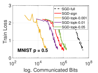
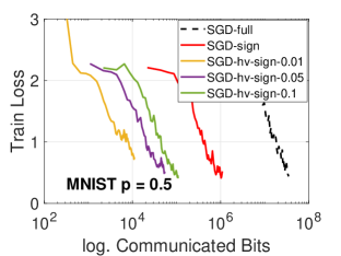
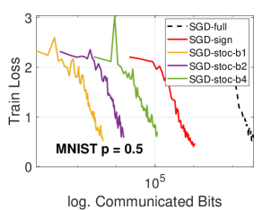
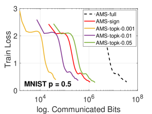
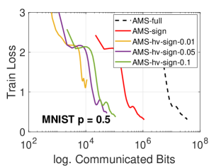
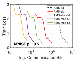
Figure 10: Training loss of Fed-EF on MNIST dataset trained by CNN. “sign”, “topk” and “hv-sign” are applied with Fed-EF, while “Stoc” is the stochastic quantization without EF. Participation rate $p=0.5$, non-iid data. 1st row: Fed-EF-SGD. 2nd row: Fed-EF-AMS.

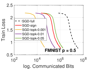
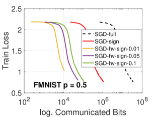
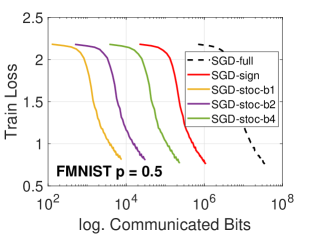
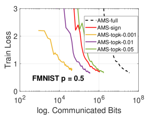
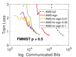
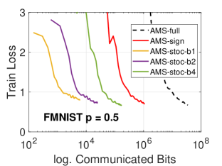
Figure 11: Training loss of Fed-EF on FMNIST dataset trained by CNN. “sign”, “topk” and “hv-sign” are applied with Fed-EF, while “Stoc” is the stochastic quantization without EF. Participation rate $p=0.5$, non-iid data. 1st row: Fed-EF-SGD. 2nd row: Fed-EF-AMS.

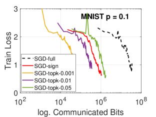
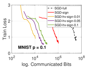
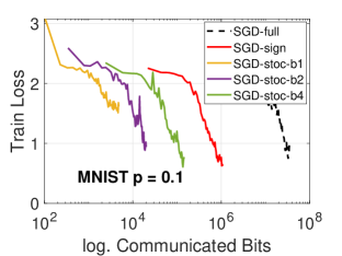
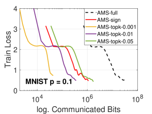
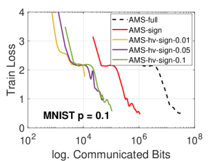
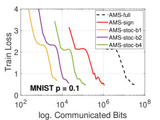
Figure 12: Training loss of Fed-EF on MNIST dataset trained by CNN. “sign”, “topk” and “hv-sign” are applied with Fed-EF, while “Stoc” is the stochastic quantization without EF. Participation rate $p=0.1$, non-iid data. 1st row: Fed-EF-SGD. 2nd row: Fed-EF-AMS.

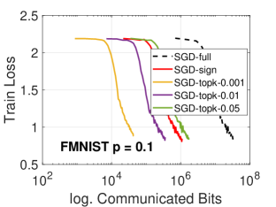
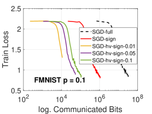
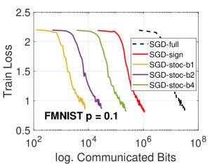
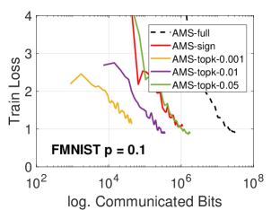
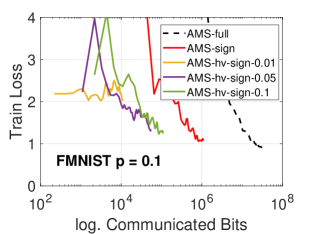
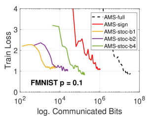
Figure 13: Training loss of Fed-EF on FMNIST dataset trained by CNN. “sign”, “topk” and “hv-sign” are applied with Fed-EF, while “Stoc” is the stochastic quantization without EF. Participation rate $p=0.1$, non-iid data. 1st row: Fed-EF-SGD. 2nd row: Fed-EF-AMS.

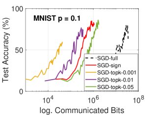
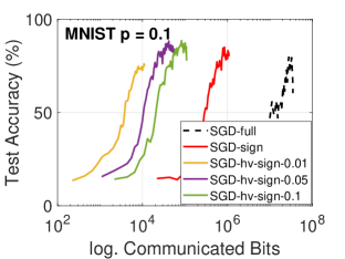
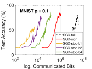
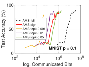
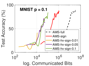
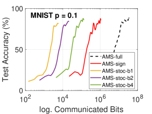
Figure 14: Test accuracy of Fed-EF on MNIST dataset trained by CNN. “sign”, “topk” and “hv-sign” are applied with Fed-EF, while “Stoc” is the stochastic quantization without EF. Participation rate $p=0.1$, non-iid data. 1st row: Fed-EF-SGD. 2nd row: Fed-EF-AMS.

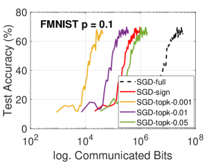
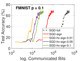
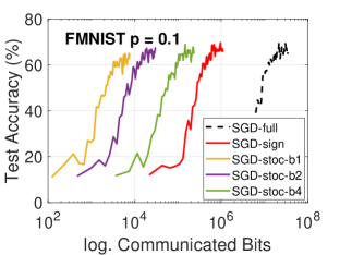
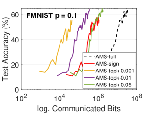
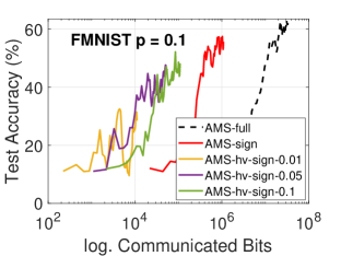
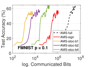
Figure 15: Test accuracy of Fed-EF on FMNIST dataset trained by CNN. “sign”, “topk” and “hv-sign” are applied with Fed-EF, while “Stoc” is the stochastic quantization without EF. Participation rate $p=0.1$, non-iid data. 1st row: Fed-EF-SGD. 2nd row: Fed-EF-AMS.

Appendix C Compression Discrepancy

In our theoretical analysis for Fed-EF, Assumption 3 is needed, which states that $\mathbb{E}[\|\frac{1}{n}\sum_{i=1}^{n}\mathcal{C}\big{(}\Delta_{t,i}+e_{t,i}\big{)}-\frac{1}{n}\sum_{i=1}^{n}(\Delta_{t,i}+e_{t,i})\|^{2}]\leq q_{\mathcal{A}}^{2}\mathbb{E}[\|\frac{1}{n}\sum_{i=1}^{n}(\Delta_{t,i}+e_{t,i})\|^{2}]$ for some $q_{\mathcal{A}}<1$ during training. In the following, we justify this assumption to demonstrate how it holds in practice. It is worth mentioning that a similar condition is was assumed in Haddadpour et al. (2021) for the analysis of FL with unbiased compression. To study sparsified SGD, Alistarh et al. (2018) also used a similar and stronger (uniform bound instead of in expectation) analytical assumption. As a result, our analysis and theoretical results are also valid under their assumption.

C.1 Simulated Data

We first conduct a simulation to investigate how the two compressors, TopK and Sign, affect $q_{\mathcal{A}}$. In our presented results, for conciseness we use $n=5$ clients and model dimensionality $d=1100$. Similar conclusions hold for much larger $n$ and $d$. We simulate two types of gradients following normal distribution and Laplace distribution (more heavy-tailed), respectively. Examples of the simulated gradients are visualized in Figure 16 and Figure 17. To mimic non-iid data, we assume that each client has some strong signals (large gradients) in some coordinates, and we scale those gradients by a scaling factor $s=2,10,100$. Conceptually, larger $s$ represents higher data heterogeneity.

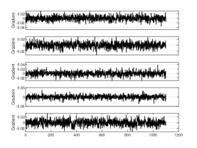
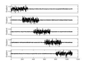
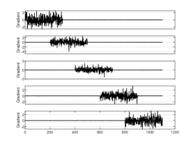
Figure 16: The simulated gradients of 5 heterogeneous clients, from $N(0,\gamma^{2})$ with $\gamma=0.01$. The gradient on each distinct client is scaled by $s=2,10,100$ (left, mid, right), respectively. Larger $s$ implies higher data heterogeneity.

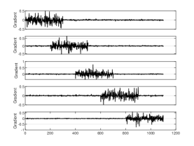
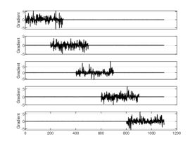
Figure 17: The simulated gradients of 5 heterogeneous clients, from $Lap(0,\lambda)$ with $\lambda=0.01$. The $x$-axis is the dimension. The gradient on each distinct client is scaled by $s=2,10,100$ (left, mid, right), respectively. Wee the gradients have heavier tail than normal distribution. Larger $s$ implies higher data heterogeneity.

We apply the TopK-0.1 and Sign compressor in Definition 1 to the simulated gradients, and compute the averaged $q_{\mathcal{A}}^{2}$ in Figure 18 over $10^{5}$ independent runs. The dashed curves are respectively the “ideal” compression coefficients $q_{\mathcal{C}}$ such that $\mathbb{E}[\|\mathcal{C}\big{(}\frac{1}{n}\sum_{i=1}^{n}\Delta_{t,i}+e_{t,i}\big{)}-\frac{1}{n}\sum_{i=1}^{n}(\Delta_{t,i}+e_{t,i})\|^{2}]\leq q_{\mathcal{C}}^{2}\mathbb{E}[\|\frac{1}{n}\sum_{i=1}^{n}(\Delta_{t,i}+e_{t,i})\|^{2}]$ from Definition 1. We see that in all cases, $q_{\mathcal{A}}$ is indeed less than 1. This still holds even when the data heterogeneity increases to as large as 100.

     

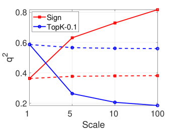
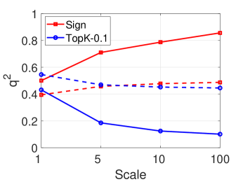
Figure 18: The compression coefficient $q_{\mathcal{A}}$ in Assumption 3 on simulated gradients. TopK is applied with sparsity $k=0.1$. Left: Gaussian distribution. Right: Laplace distribution. $q_{\mathcal{A}}^{2}$ is computed by $q=\frac{\|\delta(x)-x\|^{2}}{\|x\|^{2}}$ where $\delta(x)=\frac{1}{n}\sum_{i=1}^{n}\mathcal{C}(\Delta_{t,i}+e_{t,i})$ and $x=\frac{1}{n}\sum_{i=1}^{n}(\Delta_{t,i}+e_{t,i})$. The dashed curves are respectively the compression coefficients $q_{\mathcal{C}}^{2}$ from Definition 1, which is calculated by replacing $\delta(x)=\mathcal{C}(\frac{1}{n}\sum_{i=1}^{n}\Delta_{t,i}+e_{t,i})$. We see that in all cases, $q_{\mathcal{A}}<1$.

C.2 Real-world Data

We report the empirical $q_{\mathcal{A}}$ values when training CNN on MNIST and FMNIST datasets. The experimental setup is the same as in Section 5. We present the result in Figure 19 with $\eta=1$, $\eta_{l}=0.01$ under the same heterogeneous setting where client data are highly non-iid. The plots for other learning rate combinations and iid data are similar. In particular, we see for both compressors and both datasets, the empirical $q_{\mathcal{A}}$ is well-bounded below 1 throughout the training process.

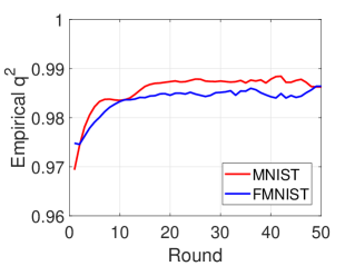
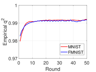
Figure 19: The compression coefficient $q_{\mathcal{A}}$ in Assumption 3 in our experiments (Section 5) for CNN trained on MNIST and FMNIST dataset, averaged over multiple runs. $\eta=1$, $\eta_{l}=0.01$, non-iid client data distribution. Left: Sign compression. Mid: TopK compression with $k=0.01$. Right: TopK compression with $k=0.1$.

Appendix D Proof of Convergence Results

We first present the proof for the more complicated Fed-EF-AMS in Section D.1, and the proof of Fed-EF-SGD would follow in Section D.2. Section D.3 contains intermediary lemmas, Section D.4 provides the analysis of Fed-EF in partial participation and Section D.5 proves the rate of FL directly using biased compression.

D.1 Proof of Theorem 4.3: Fed-EF-AMS

Proof.

We first clarify some notations. At round $t$, let the full-precision local model update of the $i$-th worker be $\Delta_{t,i}$, the error accumulator be $e_{t,i}$, and denote $\widetilde{\Delta}_{t,i}=\mathcal{C}(g_{t,i}+e_{t,i})$. Define $\bar{\Delta}_{t}=\frac{1}{n}\sum_{i=1}^{n}\Delta_{t,i}$, $\overline{\widetilde{\Delta}}_{t}=\frac{1}{n}\sum_{i=1}^{n}\widetilde{\Delta}_{t,i}$ and $\bar{e}_{t}=\frac{1}{n}\sum_{i=1}^{n}e_{t,i}$. The second moment computed by the compressed local model updates is denoted as $v_{t}=\beta_{2}v_{t-1}+(1-\beta_{2})\overline{\widetilde{\Delta}}_{t}^{2}$, and $\hat{v}_{t}=\max\{\hat{v}_{t-1},v_{t}\}$. Also, the first order moving average sequence

$$m_{t}=\beta_{1}m_{t-1}+(1-\beta_{1})\overline{\widetilde{\Delta}}_{t}\quad \textrm{and}\quad m_{t}^{\prime}=\beta_{1}m_{t-1}^{\prime}+(1-\beta_{1})\bar{\Delta}_{t},$$

where $m_{t}^{\prime}$ represents the first moment moving average sequence using the uncompressed updates. By construction we have $m_{t}^{\prime}=(1-\beta_{1})\sum_{\tau=1}^{t}\beta_{1}^{t-\tau}\bar{\Delta}_{\tau}$.

Our proof will use the following auxiliary sequences: for round $t=1,...,T$,

$$\mathcal{E}_{t+1}\mathrel{\mathop{:}}=(1-\beta_{1})\sum_{\tau=1}^{t+1}\beta_{1}^{t+1-\tau}\bar{e}_{\tau},$$

$$\theta_{t+1}^{\prime}:=\theta_{t+1}-\eta\frac{\mathcal{E}_{t+1}}{\sqrt{\hat{v}_{t}+\epsilon}}.$$

Then, we can write the evolution of $\theta_{t}^{\prime}$ as

$$\theta_{t+1}^{\prime} =\theta_{t+1}-\eta\frac{\mathcal{E}_{t+1}}{\sqrt{\hat{v}_{t}+\epsilon}}$$

$$=\theta_{t}-\eta\frac{(1-\beta_{1})\sum_{\tau=1}^{t}\beta_{1}^{t-\tau}\overline{\widetilde{\Delta}}_{\tau}+(1-\beta_{1})\sum_{\tau=1}^{t+1}\beta_{1}^{t+1-\tau}\bar{e}_{\tau}}{\sqrt{\hat{v}_{t}+\epsilon}}$$

$$=\theta_{t}-\eta\frac{(1-\beta_{1})\sum_{\tau=1}^{t}\beta_{1}^{t-\tau}(\overline{\widetilde{\Delta}}_{\tau}+\bar{e}_{\tau+1})+(1-\beta)\beta_{1}^{t}\bar{e}_{1}}{\sqrt{\hat{v}_{t}+\epsilon}}$$

$$=\theta_{t}-\eta\frac{(1-\beta_{1})\sum_{\tau=1}^{t}\beta_{1}^{t-\tau}\bar{e}_{\tau}}{\sqrt{\hat{v}_{t}+\epsilon}}-\eta\frac{m_{t}^{\prime}}{\sqrt{\hat{v}_{t}+\epsilon}}$$

$$=\theta_{t}-\eta\frac{\mathcal{E}_{t}}{\sqrt{\hat{v}_{t-1}+\epsilon}}-\eta\frac{m_{t}^{\prime}}{\sqrt{\hat{v}_{t}+\epsilon}}+\eta(\frac{1}{\sqrt{\hat{v}_{t-1}+\epsilon}}-\frac{1}{\sqrt{\hat{v}_{t}+\epsilon}})\mathcal{E}_{t}$$

$$\overset{(a)}{=}\theta_{t}^{\prime}-\eta\frac{m_{t}^{\prime}}{\sqrt{\hat{v}_{t}+\epsilon}}+\eta(\frac{1}{\sqrt{\hat{v}_{t-1}+\epsilon}}-\frac{1}{\sqrt{\hat{v}_{t}+\epsilon}})\mathcal{E}_{t}$$

$$\mathrel{\mathop{:}}=\theta_{t}^{\prime}-\eta\frac{m_{t}^{\prime}}{\sqrt{\hat{v}_{t}+\epsilon}}+\eta D_{t}\mathcal{E}_{t},$$

where (a) uses the fact of error feedback that for every $i\in[n]$, $\widetilde{\Delta}_{t,i}+e_{{t+1,i}}=\Delta_{t,i}+e_{t,i}$, and $e_{t,1}=0$ at initialization. Further define the virtual iterates:

$$x_{t+1}\mathrel{\mathop{:}}=\theta_{t+1}^{\prime}-\eta\frac{\beta_{1}}{1-\beta_{1}}\frac{m_{t}^{\prime}}{\sqrt{\hat{v}_{t}+\epsilon}},$$

which follows the recurrence:

$$x_{t+1} =\theta_{t+1}^{\prime}-\eta\frac{\beta_{1}}{1-\beta_{1}}\frac{m_{t}^{\prime}}{\sqrt{\hat{v}_{t}+\epsilon}}$$

$$=\theta_{t}^{\prime}-\eta\frac{m_{t}^{\prime}}{\sqrt{\hat{v}_{t}+\epsilon}}-\eta\frac{\beta_{1}}{1-\beta_{1}}\frac{m_{t}^{\prime}}{\sqrt{\hat{v}_{t}+\epsilon}}+\eta D_{t}\mathcal{E}_{t}$$

$$=\theta_{t}^{\prime}-\eta\frac{\beta_{1}m_{t-1}^{\prime}+(1-\beta_{1})\bar{\Delta}_{t}+\frac{\beta_{1}^{2}}{1-\beta_{1}}m_{t-1}^{\prime}+\beta_{1}\bar{\Delta}_{t}}{\sqrt{\hat{v}_{t}+\epsilon}}+\eta D_{t}\mathcal{E}_{t}$$

$$=\theta_{t}^{\prime}-\eta\frac{\beta_{1}}{1-\beta_{1}}\frac{m_{t-1}^{\prime}}{\sqrt{\hat{v}_{t}+\epsilon}}-\eta\frac{\bar{\Delta}_{t}}{\sqrt{\hat{v}_{t}+\epsilon}}+\eta D_{t}\mathcal{E}_{t}$$

$$=x_{t}-\eta\frac{\bar{\Delta}_{t}}{\sqrt{\hat{v}_{t}+\epsilon}}+\eta\frac{\beta_{1}}{1-\beta_{1}}D_{t}m_{t-1}^{\prime}+\eta D_{t}\mathcal{E}_{t}.$$

The general idea is to study the convergence of the sequence $x_{t}$, and show that the difference between $x_{t}$ and $\theta_{t}$ (of interest) is small. First, by the smoothness Assumption 1, we have

$$f(x_{t+1})\leq f(x_{t})+\langle\nabla f(x_{t}),x_{t+1}-x_{t}\rangle+\frac{L}{2}\|x_{t+1}-x_{t}\|^{2}.$$

Taking expectation w.r.t. the randomness at round $t$ and re-arranging terms, we obtain

$$\mathbb{E}[f(x_{t+1})]-f(x_{t})$$

$$\leq-\eta\mathbb{E}\Big{[}\big{\langle}\nabla f(x_{t}),\frac{\bar{\Delta}_{t}}{\sqrt{\hat{v}_{t}+\epsilon}}\big{\rangle}\Big{]}+\eta\mathbb{E}\Big{[}\big{\langle}\nabla f(x_{t}),\frac{\beta_{1}}{1-\beta_{1}}D_{t}m_{t-1}^{\prime}+D_{t}\mathcal{E}_{t}\big{\rangle}\Big{]}$$

$$\hskip 144.54pt+\frac{\eta^{2}L}{2}\mathbb{E}\Big{[}\|\frac{\bar{\Delta}_{t}}{\sqrt{\hat{v}_{t}+\epsilon}}-\frac{\beta_{1}}{1-\beta_{1}}D_{t}m_{t-1}^{\prime}-D_{t}\mathcal{E}_{t}\|^{2}\Big{]}$$

$$=\underbrace{-\eta\mathbb{E}\Big{[}\big{\langle}\nabla f(\theta_{t}),\frac{\bar{\Delta}_{t}}{\sqrt{\hat{v}_{t}+\epsilon}}\big{\rangle}\Big{]}}_{I}+\underbrace{\eta\mathbb{E}\Big{[}\big{\langle}\nabla f(x_{t}),\frac{\beta_{1}}{1-\beta_{1}}D_{t}m_{t-1}^{\prime}+D_{t}\mathcal{E}_{t}\big{\rangle}\Big{]}}_{II}$$

$$\hskip 36.135pt+\underbrace{\frac{\eta^{2}L}{2}\mathbb{E}\Big{[}\|\frac{\bar{\Delta}_{t}}{\sqrt{\hat{v}_{t}+\epsilon}}-\frac{\beta_{1}}{1-\beta_{1}}D_{t}m_{t-1}^{\prime}-D_{t}\mathcal{E}_{t}\|^{2}\Big{]}}_{III}+\underbrace{\eta\mathbb{E}\Big{[}\big{\langle}\nabla f(\theta_{t})-\nabla f(x_{t}),\frac{\bar{\Delta}_{t}}{\sqrt{\hat{v}_{t}+\epsilon}}\big{\rangle}\Big{]}}_{IV},$$ (5)

Bounding term I. We have

$$\bm{I} =-\eta\mathbb{E}\Big{[}\big{\langle}\nabla f(\theta_{t}),\frac{\bar{\Delta}_{t}}{\sqrt{\hat{v}_{t-1}+\epsilon}}\big{\rangle}\Big{]}-\eta\mathbb{E}\Big{[}\big{\langle}\nabla f(\theta_{t}),(\frac{1}{\sqrt{\hat{v}_{t}+\epsilon}}-\frac{1}{\sqrt{\hat{v}_{t-1}+\epsilon}})\bar{\Delta}_{t}\big{\rangle}\Big{]}$$

$$\leq-\eta\mathbb{E}\Big{[}\big{\langle}\nabla f(\theta_{t}),\frac{\bar{\Delta}_{t}}{\sqrt{\hat{v}_{t-1}+\epsilon}}\big{\rangle}\Big{]}+\eta\eta_{l}KG^{2}\mathbb{E}[\|D_{t}\|_{1}],$$ (6)

where we use Assumption 4 on the stochastic gradient magnitude. The last inequality holds by simply bounding the aggregated local model update by

$$\|\bar{\Delta}_{t}\|\leq\frac{1}{n}\sum_{i=1}^{n}\|\eta_{l}\sum_{k=1}^{K}g_{t,i}^{(k)}\|\leq\eta_{l}KG,$$

and the fact that for any vector in $\mathbb{R}^{d}$, the $l_{2}$ norm is upper bounded by the $l_{1}$ norm.

Regarding the first term in (6), we have

$$-\eta\mathbb{E}\Big{[}\langle\nabla f(\theta_{t}),\frac{\bar{\Delta}_{t}}{\sqrt{\hat{v}_{t-1}+\epsilon}}\Big{]}=-\eta\mathbb{E}\Big{[}\langle\frac{\nabla f(\theta_{t})}{\sqrt{\hat{v}_{t-1}+\epsilon}},\bar{\Delta}_{t}-\eta_{l}K\nabla f(\theta_{t})+\eta_{l}K\nabla f(\theta_{t})\rangle\Big{]}$$

$$=-\eta\eta_{l}K\mathbb{E}\Big{[}\frac{\|\nabla f(\theta_{t})\|^{2}}{\sqrt{\hat{v}_{t-1}+\epsilon}}\Big{]}+\eta\mathbb{E}\Big{[}\langle\frac{\nabla f(\theta_{t})}{\sqrt{\hat{v}_{t-1}+\epsilon}},-\bar{\Delta}_{t}+\eta_{l}K\nabla f(\theta_{t})\rangle\Big{]}$$

$$\overset{(a)}{\leq}-\frac{\eta\eta_{l}K}{\sqrt{\frac{4\eta_{l}^{2}(1+q^{2})^{3}K^{2}}{(1-q^{2})^{2}}G^{2}+\epsilon}}\mathbb{E}\big{[}\|\nabla f(\theta_{t})\|^{2}\big{]}+\eta\big{\langle}\frac{\nabla f(\theta_{t})}{\sqrt{\hat{v}_{t-1}+\epsilon}},\mathbb{E}\big{[}-\frac{1}{n}\sum_{i=1}^{n}\sum_{k=1}^{K}\eta_{l}g_{t,i}^{(k)}+\eta_{l}K\nabla f(\theta_{t})\big{]}\big{\rangle}$$

$$\overset{(b)}{=}-\frac{\eta\eta_{l}K}{\sqrt{\frac{4\eta_{l}^{2}(1+q^{2})^{3}K^{2}}{(1-q^{2})^{2}}G^{2}+\epsilon}}\mathbb{E}\big{[}\|\nabla f(\theta_{t})\|^{2}\big{]}$$

$$\hskip 86.72377pt+\eta\underbrace{\big{\langle}\frac{\sqrt{\eta_{l}}\nabla f(\theta_{t})}{(\hat{v}_{t-1}+\epsilon)^{1/4}},\mathbb{E}\Big{[}\frac{\sqrt{\eta_{l}}}{n(\hat{v}_{t-1}+\epsilon)^{1/4}}(-\sum_{i=1}^{n}\sum_{k=1}^{K}\nabla f_{i}(\theta_{t,i}^{(k)})+K\nabla f(\theta_{t}))\Big{]}\big{\rangle}}_{V},$$

where (a) uses Lemma D.7 and (b) is due to Assumption 2 that $g_{t,i}^{(k)}$ is an unbiased estimator of $\nabla f_{i}(\theta_{t,i}^{(k)})$. To bound term V, we use the similar proof structure as in the proof of Lemma D.3. Specifically, we have

$$\bm{V} \leq\frac{\eta_{l}K}{2\sqrt{\epsilon}}\mathbb{E}\big{[}\|\nabla f(\theta_{t})\|^{2}\big{]}+\frac{\eta_{l}}{2K\sqrt{\epsilon}}\mathbb{E}\big{[}\|\frac{1}{n}\sum_{i=1}^{n}\sum_{k=1}^{K}(\nabla f_{i}(\theta_{t,i}^{(k)})-\nabla f_{i}(\theta_{t}))\|^{2}\big{]}$$

$$\leq\frac{\eta_{l}K}{2\sqrt{\epsilon}}\mathbb{E}\big{[}\|\nabla f(\theta_{t})\|^{2}\big{]}+\frac{\eta_{l}}{2nK\sqrt{\epsilon}}\mathbb{E}\big{[}\sum_{i=1}^{n}\|\sum_{k=1}^{K}(\nabla f_{i}(\theta_{t,i}^{(k)})-\nabla f_{i}(\theta_{t}))\|^{2}\big{]}$$

$$\leq\frac{\eta_{l}K}{2\sqrt{\epsilon}}\mathbb{E}\big{[}\|\nabla f(\theta_{t})\|^{2}\big{]}+\frac{\eta_{l}}{2n\sqrt{\epsilon}}\mathbb{E}\big{[}\sum_{i=1}^{n}\sum_{k=1}^{K}\|\nabla f_{i}(\theta_{t,i}^{(k)})-\nabla f_{i}(\theta_{t})\|^{2}\big{]}$$

$$\leq\frac{\eta_{l}K}{2\sqrt{\epsilon}}\mathbb{E}\big{[}\|\nabla f(\theta_{t})\|^{2}\big{]}+\frac{\eta_{l}L^{2}}{2n\sqrt{\epsilon}}\mathbb{E}\big{[}\sum_{i=1}^{n}\sum_{k=1}^{K}\|\theta_{t,i}^{(k)}-\theta_{t}\|^{2}\big{]},$$

where the last inequality is a result of the $L$-smoothness assumption on the loss function $f_{i}(x)$. Applying Lemma D.1 to the consensus error, we can further bound term $V$ by

$$\bm{V} \leq\frac{\eta_{l}K}{2\sqrt{\epsilon}}\mathbb{E}\big{[}\|\nabla f(\theta_{t})\|^{2}\big{]}+\frac{\eta_{l}KL^{2}}{2\sqrt{\epsilon}}\big{[}5\eta_{l}^{2}K(\sigma^{2}+6K\sigma_{g}^{2})+30\eta_{l}^{2}K^{2}\mathbb{E}[\|\nabla f(\theta_{t})\|^{2}]\big{]}$$

$$\leq\frac{47\eta_{l}K}{64\sqrt{\epsilon}}\mathbb{E}\big{[}\|\nabla f(\theta_{t})\|^{2}\big{]}+\frac{5\eta_{l}^{3}K^{2}L^{2}}{2\sqrt{\epsilon}}(\sigma^{2}+6K\sigma_{g}^{2}),$$

when we choose $\eta_{l}\leq\frac{1}{8KL}$. Further, if we set $\eta_{l}\leq\frac{\sqrt{15}(1-q^{2})\sqrt{\epsilon}}{14(1+q^{2})^{1.5}KG}$, we have

$$\frac{4\eta_{l}^{2}(1+q^{2})^{3}K^{2}}{(1-q^{2})^{2}}G^{2}+\epsilon\leq\frac{60}{196}\epsilon+\epsilon=\frac{64}{49}\epsilon.$$

Hence, as $\frac{47}{64}<\frac{3}{4}$, we can establish from (6) that

$$\bm{I}\leq-\frac{\eta\eta_{l}K}{8\sqrt{\epsilon}}\mathbb{E}\big{[}\|\nabla f(\theta_{t})\|^{2}\big{]}+\frac{5\eta\eta_{l}^{3}K^{2}L^{2}}{2\sqrt{\epsilon}}(\sigma^{2}+6K\sigma_{g}^{2})+\eta\eta_{l}KG^{2}\mathbb{E}[\|D_{t}\|_{1}].$$ (7)

Bounding term II. By Lemma D.6, we know that $\|\mathcal{E}_{t}\|\leq\frac{2\eta_{l}qKG}{1-q^{2}}$, and by Lemma D.4, $\|m_{t}^{\prime}\|\leq\eta_{l}KG$. Thus, we have

$$\bm{II} \leq\eta\Big{(}\mathbb{E}\big{[}\langle\nabla f(\theta_{t}),\frac{\beta_{1}}{1-\beta_{1}}D_{t}m_{t-1}^{\prime}+D_{t}\mathcal{E}_{t}\rangle\big{]}+\mathbb{E}\big{[}\langle\nabla f(x_{t})-\nabla f(\theta_{t}),\frac{\beta_{1}}{1-\beta_{1}}D_{t}m_{t-1}^{\prime}+D_{t}\mathcal{E}_{t}\rangle\big{]}\Big{)}$$

$$\leq\eta\mathbb{E}\big{[}\|\nabla f(\theta_{t})\|\|\frac{\beta_{1}}{1-\beta_{1}}D_{t}m_{t-1}^{\prime}+D_{t}\mathcal{E}_{t}\|\big{]}$$

$$\hskip 108.405pt+\eta^{2}\ L\mathbb{E}\big{[}\|\frac{\frac{\beta_{1}}{1-\beta_{1}}m_{t-1}^{\prime}+\mathcal{E}_{t}}{\sqrt{\hat{v}_{t-1}+\epsilon}}\|\|\frac{\beta_{1}}{1-\beta_{1}}D_{t}m_{t-1}^{\prime}+D_{t}\mathcal{E}_{t}\|\big{]}$$

$$\leq\eta\eta_{l}C_{1}KG^{2}\mathbb{E}[\|D_{t}\|_{1}]+\frac{\eta^{2}\eta_{l}^{2}C_{1}^{2}LK^{2}G^{2}}{\sqrt{\epsilon}}\mathbb{E}[\|D_{t}\|_{1}],$$ (8)

where $C_{1}\mathrel{\mathop{:}}=\frac{\beta_{1}}{1-\beta_{1}}+\frac{2q}{1-q^{2}}$, and the second inequality is due to the smoothness of $f(\theta)$.

Bounding term III. This term can be bounded as follows:

$$\bm{III} \leq\eta^{2}L\mathbb{E}\big{[}\|\frac{\bar{\Delta}_{t}}{\sqrt{\hat{v}_{t}+\epsilon}}\|^{2}\big{]}+\eta^{2}L\mathbb{E}\big{[}\|\frac{\beta_{1}}{1-\beta_{1}}D_{t}m_{t-1}^{\prime}-D_{t}\mathcal{E}_{t}\|^{2}\big{]}$$

$$\leq\frac{\eta^{2}L}{\epsilon}\mathbb{E}\big{[}\|\bar{\Delta}_{t}\|^{2}\big{]}+\eta^{2}L\mathbb{E}\big{[}\|D_{t}(\frac{\beta_{1}}{1-\beta_{1}}m_{t-1}^{\prime}-\mathcal{E}_{t})\|^{2}\big{]}$$

$$\leq\frac{\eta^{2}L(2\eta_{l}^{2}K^{2}+120\eta_{l}^{4}K^{4}L^{2})}{\epsilon}\mathbb{E}\big{[}\|\nabla f(\theta_{t})\|^{2}\big{]}+\frac{4\eta^{2}\eta_{l}^{2}KL}{n\epsilon}\sigma^{2}$$

$$\hskip 86.72377pt+\frac{20\eta^{2}\eta_{l}^{4}K^{3}L^{3}}{\epsilon}(\sigma^{2}+6K\sigma_{g}^{2})+\eta^{2}\eta_{l}^{2}C_{1}^{2}LK^{2}G^{2}\mathbb{E}[\|D_{t}\|^{2}],$$ (9)

where we apply Lemma D.2 and use similar argument as in bounding term II.

Bounding term IV. Lastly, for term IV, we have for some $\rho>0$,

$$\bm{IV} =\eta\mathbb{E}\Big{[}\big{\langle}\nabla f(\theta_{t})-\nabla f(x_{t}),\frac{\bar{\Delta}_{t}}{\sqrt{\hat{v}_{t-1}+\epsilon}}\big{\rangle}\Big{]}+\eta\mathbb{E}\Big{[}\big{\langle}\nabla f(\theta_{t})-\nabla f(x_{t}),(\frac{1}{\sqrt{\hat{v}_{t}+\epsilon}}-\frac{1}{\sqrt{\hat{v}_{t-1}+\epsilon}})\bar{\Delta}_{t}\big{\rangle}\Big{]}$$

$$\overset{(a)}{\leq}\frac{\eta\rho}{2\epsilon}\mathbb{E}\big{[}\|\bar{\Delta}_{t}\|^{2}\big{]}+\frac{\eta}{2\rho}\mathbb{E}\big{[}\|\nabla f(\theta_{t})-\nabla f(x_{t})\|^{2}\big{]}+\eta^{2}L\mathbb{E}\Big{[}\|\frac{\frac{\beta_{1}}{1-\beta_{1}}m_{t-1}^{\prime}+\mathcal{E}_{t}}{\sqrt{\hat{v}_{t-1}+\epsilon}}\|\|D_{t}\Delta_{t}\|\Big{]}$$

$$\overset{(b)}{\leq}\frac{\rho\eta(\eta_{l}^{2}K^{2}+60\eta_{l}^{4}K^{4}L^{2})}{\epsilon}\mathbb{E}\big{[}\|\nabla f(\theta_{t})\|^{2}\big{]}+\frac{2\rho\eta\eta_{l}^{2}K}{\epsilon n}\sigma^{2}+\frac{10\rho\eta\eta_{l}^{4}K^{3}L^{2}}{\epsilon}(\sigma^{2}+6K\sigma_{g}^{2})$$

$$\hskip 130.08621pt+\frac{\eta^{3}L^{2}}{2\rho}\mathbb{E}\Big{[}\|\frac{\frac{\beta_{1}}{1-\beta_{1}}m_{t-1}^{\prime}+\mathcal{E}_{t}}{\sqrt{\hat{v}_{t-1}+\epsilon}}\|^{2}\Big{]}+\frac{\eta^{2}\eta_{l}^{2}C_{1}LK^{2}G^{2}}{\sqrt{\epsilon}}\mathbb{E}[\|D_{t}\|]$$

$$\leq\frac{\rho\eta\eta_{l}^{2}K^{2}(60\eta_{l}^{2}K^{2}L^{2}+1)}{\epsilon}\mathbb{E}\big{[}\|\nabla f(\theta_{t})\|^{2}\big{]}+\frac{2\rho\eta\eta_{l}^{2}K}{\epsilon n}\sigma^{2}+\frac{10\rho\eta\eta_{l}^{4}K^{3}L^{2}}{\epsilon}(\sigma^{2}+6K\sigma_{g}^{2})$$

$$\hskip 57.81621pt+\frac{\eta^{3}L^{2}}{\rho\epsilon}\Big{[}\frac{\beta_{1}^{2}}{(1-\beta_{1})^{2}}\mathbb{E}\big{[}\|m_{t}^{\prime}\|^{2}\big{]}+\mathbb{E}\big{[}\|\mathcal{E}_{t}\|^{2}\big{]}\Big{]}+\frac{\eta^{2}\eta_{l}^{2}C_{1}LK^{2}G^{2}}{\sqrt{\epsilon}}\mathbb{E}[\|D_{t}\|_{1}],$$ (10)

where (a) is a consequence of Young’s inequality ($\rho$ will be specified later) and the smoothness Assumption 1, and (b) is based on Lemma D.2.

After we have bounded all four terms in (5), the next step is to gather the ingredients by taking the telescope sum over $t=1,...,T$. For the ease of presentation, we first do this for the third term in (10). According to Lemma D.4 and Lemma D.6, summing over $t=1,...,T$, we conclude

$$\sum_{t=1}^{T}\frac{\eta^{3}L^{2}}{\rho\epsilon}\Big{[}\frac{\beta_{1}^{2}}{(1-\beta_{1})^{2}}\mathbb{E}[\|m_{t}^{\prime}\|^{2}]+\mathbb{E}[\|\mathcal{E}_{t}\|^{2}]\Big{]}$$

$$\leq\frac{\eta^{3}\beta_{1}^{2}L^{2}}{\rho(1-\beta_{1})^{2}\epsilon}\Big{[}2\eta_{l}^{2}K^{2}(60\eta_{l}^{2}K^{2}L^{2}+1)\sum_{t=1}^{T}\mathbb{E}\big{[}\|\nabla f(\theta_{t})\|^{2}\big{]}+4\frac{T\eta_{l}^{2}K}{n}\sigma^{2}+20T\eta_{l}^{4}K^{3}L^{2}(\sigma^{2}+6K\sigma_{g}^{2})\Big{]}$$

$$+\frac{\eta^{3}q^{2}L^{2}}{\rho(1-q^{2})^{2}\epsilon}\Big{[}8\eta_{l}^{2}K^{2}(60\eta_{l}^{2}K^{2}L^{2}+1)\sum_{t=1}^{T}\mathbb{E}\big{[}\|\nabla f(\theta_{\tau})\|^{2}\big{]}+\frac{16T\eta_{l}^{2}K}{n}\sigma^{2}+80T\eta_{l}^{4}K^{3}L^{2}(\sigma^{2}+6K\sigma_{g}^{2})\Big{]}$$

$$\leq\frac{2\eta^{3}\eta_{l}^{2}C_{2}K^{2}L^{2}}{\rho\epsilon}(60\eta_{l}^{2}K^{2}L^{2}+1)\sum_{t=1}^{T}\mathbb{E}\big{[}\|\nabla f(\theta_{t})\|^{2}\big{]}$$

$$\hskip 108.405pt+\frac{4T\eta^{3}\eta_{l}^{2}C_{2}KL^{2}}{\rho n\epsilon}\sigma^{2}+\frac{20T\eta^{3}\eta_{l}^{4}C_{2}K^{3}L^{4}}{\rho\epsilon}(\sigma^{2}+6K\sigma_{g}^{2}),$$ (11)

with $C_{2}\mathrel{\mathop{:}}=\frac{\beta_{1}^{2}}{(1-\beta_{1})^{2}}+\frac{4q^{2}}{(1-q^{2})^{2}}$.

Putting together. We are in the position to combine pieces together to get our final result by integrating (7), (8), (9), (10) and (11) into (5) and taking the telescoping sum over $t=1,...,T$. After re-arranging terms, when $\eta_{l}\leq\min\big{\{}\frac{1}{8KL},\frac{(1-q^{2})\sqrt{\epsilon}}{4(1+q^{2})^{1.5}KG}\big{\}}$, we have

$$\mathbb{E}[f(x_{T+1})-f(x_{1})]$$

$$\leq-\frac{\eta\eta_{l}K}{8\sqrt{\epsilon}}\sum_{t=1}^{T}\mathbb{E}\big{[}\|\nabla f(\theta_{t})\|^{2}\big{]}+\frac{5T\eta\eta_{l}^{3}K^{2}L^{2}}{2\sqrt{\epsilon}}(\sigma^{2}+6K\sigma_{g}^{2})+\eta\eta_{l}KG^{2}\sum_{t=1}^{T}\mathbb{E}[\|D_{t}\|_{1}]$$

$$+\eta\eta_{l}C_{1}KG^{2}\sum_{t=1}^{T}\mathbb{E}[\|D_{t}\|_{1}]+\frac{\eta^{2}\eta_{l}^{2}C_{1}^{2}LK^{2}G^{2}}{\sqrt{\epsilon}}\sum_{t=1}^{T}\mathbb{E}[\|D_{t}\|_{1}]$$

$$+\frac{\eta^{2}L(2\eta_{l}^{2}K^{2}+120\eta_{l}^{4}K^{4}L^{2})}{\epsilon}\sum_{t=1}^{T}\mathbb{E}\big{[}\|\nabla f(\theta_{t})\|^{2}\big{]}+\frac{4T\eta^{2}\eta_{l}^{2}KL}{n\epsilon}\sigma^{2}$$

$$\hskip 86.72377pt+\frac{20T\eta^{2}\eta_{l}^{4}K^{3}L^{3}}{\epsilon}(\sigma^{2}+6K\sigma_{g}^{2})+\eta^{2}\eta_{l}^{2}C_{1}^{2}LK^{2}G^{2}\sum_{t=1}^{T}\mathbb{E}[\|D_{t}\|^{2}]$$

$$+\frac{\rho\eta\eta_{l}^{2}K^{2}(60\eta_{l}^{2}K^{2}L^{2}+1)}{\epsilon}\sum_{t=1}^{T}\mathbb{E}\big{[}\|\nabla f(\theta_{t})\|^{2}\big{]}+\frac{2T\rho\eta\eta_{l}^{2}K}{\epsilon n}\sigma^{2}+\frac{10T\rho\eta\eta_{l}^{4}K^{3}L^{2}}{\epsilon}(\sigma^{2}+6K\sigma_{g}^{2})$$

$$+\frac{2\eta^{3}\eta_{l}^{2}C_{2}K^{2}L^{2}}{\rho\epsilon}(60\eta_{l}^{2}K^{2}L^{2}+1)\sum_{t=1}^{T}\mathbb{E}\big{[}\|\nabla f(\theta_{t})\|^{2}\big{]}+\frac{4T\eta^{3}\eta_{l}^{2}C_{2}KL^{2}}{\rho n\epsilon}\sigma^{2}$$

$$\hskip 108.405pt+\frac{20T\eta^{3}\eta_{l}^{4}C_{2}K^{3}L^{4}}{\rho\epsilon}(\sigma^{2}+6K\sigma_{g}^{2})+\frac{\eta^{2}\eta_{l}^{2}C_{1}LK^{2}G^{2}}{\sqrt{\epsilon}}\sum_{t=1}^{T}\mathbb{E}[\|D_{t}\|_{1}]$$

$$=\Upsilon_{1}\cdot\sum_{t=1}^{T}\mathbb{E}\big{[}\|\nabla f(\theta_{t})\|^{2}\big{]}+\Upsilon_{2}\cdot(\sigma^{2}+6K\sigma_{g}^{2})+\Upsilon_{3}\cdot\sigma^{2}$$

$$\hskip 108.405pt+\Upsilon_{4}\cdot\sum_{t=1}^{T}\mathbb{E}[\|D_{t}\|_{1}]+\eta^{2}\eta_{l}^{2}C_{1}^{2}LK^{2}G^{2}\sum_{t=1}^{T}\mathbb{E}[\|D_{t}\|^{2}],$$ (12)

where

$$\Upsilon_{1} =-\frac{\eta\eta_{l}K}{8\sqrt{\epsilon}}+\frac{\eta^{2}L(2\eta_{l}^{2}K^{2}+120\eta_{l}^{4}K^{4}L^{2})}{\epsilon}$$

$$\hskip 86.72377pt+\frac{\rho\eta\eta_{l}^{2}K^{2}(60\eta_{l}^{2}K^{2}L^{2}+1)}{\epsilon}+\frac{2\eta^{3}\eta_{l}^{2}C_{2}K^{2}L^{2}}{\rho\epsilon}(60\eta_{l}^{2}K^{2}L^{2}+1)$$

$$\leq-\frac{\eta\eta_{l}K}{8\sqrt{\epsilon}}+\frac{2\eta^{2}\eta_{l}^{2}K^{2}L}{\epsilon}+\frac{120\eta^{2}\eta_{l}^{4}K^{4}L^{3}}{\epsilon}+\frac{2\rho\eta\eta_{l}^{2}K^{2}}{\epsilon}+\frac{4\eta^{3}\eta_{l}^{2}C_{2}K^{2}L^{2}}{\rho\epsilon},$$ (13)

$$\Upsilon_{2} =\frac{5T\eta\eta_{l}^{3}K^{2}L^{2}}{2\sqrt{\epsilon}}+\frac{20T\eta^{2}\eta_{l}^{4}K^{3}L^{3}}{\epsilon}+\frac{10T\rho\eta\eta_{l}^{4}K^{3}L^{2}}{\epsilon}+\frac{20T\eta^{3}\eta_{l}^{4}C_{2}K^{3}L^{4}}{\rho\epsilon},$$

$$\Upsilon_{3} =\frac{4T\eta^{2}\eta_{l}^{2}KL}{n\epsilon}+\frac{2T\rho\eta\eta_{l}^{2}K}{n\epsilon}+\frac{4T\eta^{3}\eta_{l}^{2}C_{2}KL^{2}}{\rho n\epsilon},$$

$$\Upsilon_{4} =\eta\eta_{l}(C_{1}+1)KG^{2}+\frac{\eta^{2}\eta_{l}^{2}C_{1}^{2}LK^{2}G^{2}}{\sqrt{\epsilon}}+\frac{\eta^{2}\eta_{l}^{2}C_{1}LK^{2}G^{2}}{\sqrt{\epsilon}},$$

where to bound $\Upsilon_{1}$ we use the fact that $\eta_{l}\leq\frac{1}{8KL}$. We now look at the upper bound (13) of $\Upsilon_{1}$ which contains 5 terms. In the following, we choose $\rho\equiv L\eta$ in (10) and (11). Suppose we choose $\epsilon<1$. Then, when the local learning rate satisfies

$$\eta_{l} \leq\frac{1}{K}\min\Big{\{}\frac{1}{8L},\frac{(1-q^{2})\sqrt{\epsilon}}{4(1+q^{2})^{1.5}G},\frac{\sqrt{\epsilon}}{128\eta L},\frac{\sqrt{\epsilon}}{256C_{2}\eta L},\big{(}\frac{\sqrt{\epsilon}}{7680\eta}\big{)}^{1/3}\frac{1}{L}\Big{\}}$$

$$\leq\frac{\sqrt{\epsilon}}{8KL}\min\Big{\{}\frac{1}{\sqrt{\epsilon}},\frac{2(1-q^{2})L}{(1+q^{2})^{1.5}G},\frac{1}{\max\{16,32C_{2}\}\eta},\frac{1}{3\eta^{1/3}}\Big{\}},$$

each of the last four terms can be bounded by $\frac{\eta\eta_{l}K}{48\sqrt{\epsilon}}$. Thus, under this learning rate setting,

$$\Upsilon_{1}\leq-\frac{\eta\eta_{l}K}{16\sqrt{\epsilon}}.$$

Taking the above into (12), we arrive at

$$\frac{\eta\eta_{l}K}{16\sqrt{\epsilon}}\sum_{t=1}^{T}\mathbb{E}\big{[}\|\nabla f(\theta_{t})\|^{2}\big{]} \leq f(x_{1})-\mathbb{E}[f(x_{T+1})]+\Upsilon_{2}\cdot(\sigma^{2}+6K\sigma_{g}^{2})$$

$$\hskip 57.81621pt+\Upsilon_{3}\cdot\sigma^{2}+\Upsilon_{4}\cdot\frac{d}{\sqrt{\epsilon}}+\frac{\eta^{2}\eta_{l}^{2}C_{1}^{2}LK^{2}G^{2}d}{\epsilon},$$

where Lemma D.8 on the difference sequence $D_{t}$ is applied. Consequently, we have

$$\frac{1}{T}\sum_{t=1}^{T}\mathbb{E}\big{[}\|\nabla f(\theta_{t})\|^{2}\big{]} \lesssim\frac{f(x_{1})-\mathbb{E}[f(x_{T+1})]}{\eta\eta_{l}TK}+\widetilde{\Upsilon}_{2}\cdot(\sigma^{2}+6K\sigma_{g}^{2})+\widetilde{\Upsilon}_{3}\cdot\sigma^{2}$$

$$\hskip 50.58878pt+\frac{(C_{1}+1)G^{2}d}{T\sqrt{\epsilon}}+\frac{2\eta\eta_{l}C_{1}^{2}LKG^{2}d}{T\epsilon}+\frac{\eta\eta_{l}C_{1}^{2}LKG^{2}d}{T\epsilon}$$

$$\leq\frac{f(x_{1})-\mathbb{E}[f(x_{T+1})]}{\eta\eta_{l}TK}+\widetilde{\Upsilon}_{2}\cdot(\sigma^{2}+6K\sigma_{g}^{2})+\widetilde{\Upsilon}_{3}\cdot\sigma^{2}$$

$$\hskip 130.08621pt+\frac{(C_{1}+1)G^{2}d}{T\sqrt{\epsilon}}+\frac{3\eta\eta_{l}C_{1}^{2}LKG^{2}d}{T\epsilon},$$

where we make simplification at the second inequality using the fact that $C_{1}\leq C_{1}^{2}$ since $C_{1}\geq 1$. Moreover, $\widetilde{\Upsilon}_{2}$ and $\widetilde{\Upsilon}_{3}$ is defined as (recall that we have chosen $\rho\equiv L\eta$)

$$\widetilde{\Upsilon}_{2} =\frac{5\eta_{l}^{2}KL^{2}}{2\sqrt{\epsilon}}+\frac{20\eta\eta_{l}^{3}K^{2}L^{3}}{\epsilon}+\frac{10\eta\eta_{l}^{3}K^{2}L^{3}}{\epsilon}+\frac{20\eta\eta_{l}^{3}C_{2}K^{2}L^{3}}{\epsilon}$$

$$\leq\frac{5\eta_{l}^{2}KL^{2}}{2\sqrt{\epsilon}}+\frac{\eta\eta_{l}^{3}(30+20C_{2})K^{2}L^{3}}{\epsilon},$$

$$\widetilde{\Upsilon}_{3} =\frac{4\eta\eta_{l}L}{n\epsilon}+\frac{2\eta\eta_{l}L}{n\epsilon}+\frac{4\eta\eta_{l}C_{2}L}{n\epsilon}\leq\frac{\eta\eta_{l}L(6+4C_{2})}{n\epsilon}.$$

Finally, to connect the virtual iterates $x_{t}$ with the actual iterates $\theta_{t}$, note that $x_{1}=\theta_{1}$, and $f(x_{T+1})\geq f(\theta^{*})$ since $\theta^{*}=\arg\min_{\theta}f(\theta)$. Replacing $\widetilde{\Upsilon}_{2}$ and $\widetilde{\Upsilon}_{3}$ with above upper bounds, this eventually leads to the bound

$$\frac{1}{T}\sum_{t=1}^{T}\mathbb{E}\big{[}\|\nabla f(\theta_{t})\|^{2}\big{]} \lesssim\frac{f(\theta_{1})-f(\theta^{*})}{\eta\eta_{l}TK}+\Big{[}\frac{5\eta_{l}^{2}KL^{2}}{2\sqrt{\epsilon}}+\frac{\eta\eta_{l}^{3}(30+20C_{1}^{2})K^{2}L^{3}}{\epsilon}\Big{]}(\sigma^{2}+6K\sigma_{g}^{2})$$

$$\hskip 36.135pt+\frac{\eta\eta_{l}L(6+4C_{1}^{2})}{n\epsilon}\sigma^{2}+\frac{(C_{1}+1)G^{2}d}{T\sqrt{\epsilon}}+\frac{3\eta\eta_{l}C_{1}^{2}LKG^{2}d}{T\epsilon},$$

which gives the desired result. Here we use the fact that $C_{2}\leq C_{1}^{2}$. This completes the proof. ∎

D.2 Proof of Theorem 4.2: Fed-EF-SGD

Proof.

Now, we prove the variant of Fed-EF with SGD as the central server update rule. The proof follows the same routine as the one for Fed-EF-AMS, but is simpler since there are no moving average terms that need to be handled. Note that for this algorithm, we do not need Assumption 4 that the stochastic gradients are uniformly bounded.

For Fed-EF-SGD, consider the virtual sequence

$$x_{t+1} =\theta_{t+1}-\eta\bar{e}_{t+1}$$

$$=\theta_{t}-\eta\overline{\widetilde{\Delta}}_{t}-\eta\bar{e}_{t+1}$$

$$=\theta_{t}-\frac{\eta}{n}\sum_{i=1}^{n}(\tilde{\Delta}_{t,i}+e_{t+1,i})$$

$$=\theta_{t}-\eta\bar{\Delta}_{t}-\eta\bar{e}_{t}$$

$$=x_{t}-\eta\bar{\Delta}_{t},$$ (14)

where the second last equality follows from the update rule that $\tilde{\Delta}_{t,i}+e_{t+1,i}=\Delta_{t,i}+e_{t,i}$ for all $i\in[n]$ and $t\in[T]$.

By the smoothness Assumption 1, we have

$$f(x_{t+1})\leq f(x_{t})+\langle\nabla f(x_{t}),x_{t+1}-x_{t}\rangle+\frac{L}{2}\|x_{t+1}-x_{t}\|^{2}.$$

Taking expectation w.r.t. the randomness at round $t$ gives

$$\mathbb{E}[f(x_{t+1})]-f(x_{t})$$

$$\leq-\eta\mathbb{E}\big{[}\langle\nabla f(x_{t}),\bar{\Delta}_{t}\rangle\big{]}+\frac{\eta^{2}L}{2}\mathbb{E}\big{[}\|\bar{\Delta}_{t}\|^{2}\big{]}$$

$$=-\eta\mathbb{E}\big{[}\langle\nabla f(\theta_{t}),\bar{\Delta}_{t}\rangle\big{]}+\frac{\eta^{2}L}{2}\mathbb{E}\big{[}\|\bar{\Delta}_{t}\|^{2}\big{]}+\eta\mathbb{E}\big{[}\langle\nabla f(\theta_{t})-\nabla f(x_{t}),\bar{\Delta}_{t}\rangle\big{]}.$$ (15)

We can bound the first term in (15) using similar technique as bounding term I in the proof of Fed-EF-AMS. Specifically, we have

$$-\eta\mathbb{E}\big{[}\langle\nabla f(\theta_{t}),\bar{\Delta}_{t}\rangle\big{]} =-\eta\mathbb{E}\big{[}\langle\nabla f(\theta_{t}),\bar{\Delta}_{t}-\eta_{l}K\nabla f(\theta_{t})+\eta_{l}K\nabla f(\theta_{t})\rangle\big{]}$$

$$=-\eta\eta_{l}K\mathbb{E}\big{[}\|\nabla f(\theta_{t})\|^{2}\big{]}+\eta\mathbb{E}\big{[}\langle\nabla f(\theta_{t}),-\bar{\Delta}_{t}+\eta_{l}K\nabla f(\theta_{t})\rangle\big{]}.$$

With $\eta_{l}\leq\frac{1}{8KL}$, applying Lemma D.3, we have

$$-\eta\mathbb{E}\big{[}\langle\nabla f(\theta_{t}),\bar{\Delta}_{t}\rangle\big{]} \leq-\eta\eta_{l}K\mathbb{E}\big{[}\|\nabla f(\theta_{t})\|^{2}\big{]}+\frac{3\eta\eta_{l}K}{4}\mathbb{E}\big{[}\|\nabla f(\theta_{t})\|^{2}\big{]}+\frac{5\eta\eta_{l}^{3}K^{2}L^{2}}{2}(\sigma^{2}+6K\sigma_{g}^{2})$$

$$=-\frac{\eta\eta_{l}K}{4}\mathbb{E}\big{[}\|\nabla f(\theta_{t})\|^{2}\big{]}+\frac{5\eta\eta_{l}^{3}K^{2}L^{2}}{2}(\sigma^{2}+6K\sigma_{g}^{2}).$$

The second term in (15) can be bounded using Lemma D.2 as

$$\frac{\eta^{2}L}{2}\mathbb{E}\big{[}\|\bar{\Delta}_{t}\|^{2}\big{]} \leq\eta^{2}\eta_{l}^{2}K^{2}L(60\eta_{l}^{2}K^{2}L^{2}+1)\mathbb{E}\big{[}\|\nabla f(\theta_{t})\|^{2}\big{]}$$

$$\hskip 72.26999pt+\frac{2\eta^{2}\eta_{l}^{2}KL}{n}\sigma^{2}+10\eta^{2}\eta_{l}^{4}K^{3}L^{3}(\sigma^{2}+6K\sigma_{g}^{2}).$$

The last term in (15) can be bounded similarly as VI in Fed-EF-AMS by

$$\eta\mathbb{E}\big{[}\langle\nabla f(\theta_{t})-\nabla f(x_{t}),\bar{\Delta}_{t}\rangle\big{]}$$

$$\leq\frac{\eta\rho}{2}\mathbb{E}\big{[}\|\bar{\Delta}_{t}\|^{2}\big{]}+\frac{\eta}{2\rho}\mathbb{E}\big{[}\|\nabla f(\theta_{t})-\nabla f(x_{t})\|^{2}\big{]}$$

$$\overset{(a)}{\leq}\frac{\eta^{2}}{2}\mathbb{E}\big{[}\|\bar{\Delta}_{t}\|^{2}\big{]}+\frac{\eta^{2}L^{2}}{2}\mathbb{E}\big{[}\|\bar{e}_{t}\|^{2}\big{]}$$ (16)

$$\overset{(b)}{\leq}\frac{\eta^{2}L}{2}\Big{[}2\eta_{l}^{2}K^{2}(60\eta_{l}^{2}K^{2}L^{2}+1)\mathbb{E}\big{[}\|\nabla f(\theta_{t})\|^{2}\big{]}+4\frac{\eta_{l}^{2}K}{n}\sigma^{2}+20\eta_{l}^{4}K^{3}L^{2}(\sigma^{2}+6K\sigma_{g}^{2})\Big{]}$$

$$+\frac{\eta^{2}L}{2}\Big{[}\frac{4q^{2}\eta_{l}^{2}K^{2}(60\eta_{l}^{2}K^{2}L^{2}+1)}{1-q^{2}}\sum_{\tau=1}^{t}(\frac{1+q^{2}}{2})^{t-\tau}\mathbb{E}\big{[}\|\nabla f(\theta_{\tau})\|^{2}\big{]}$$

$$\hskip 130.08621pt+\frac{16\eta_{l}^{2}q^{2}K}{(1-q^{2})^{2}n}\sigma^{2}+\frac{80\eta_{l}^{4}q^{2}K^{3}L^{2}}{(1-q^{2})^{2}}(\sigma^{2}+6K\sigma_{g}^{2})\Big{]},$$

where (a) uses Young’s inequality and (b) uses Lemma D.2 and Lemma D.5. When taking telescoping sum of this term over $t=1,...,T$, again using the geometric summation trick, we further obtain

$$\eta\sum_{t=1}^{T}\mathbb{E}\big{[}\langle\nabla f(\theta_{t})-\nabla f(x_{t}),\bar{\Delta}_{t}\rangle\big{]}$$

$$\leq\eta^{2}\eta_{l}^{2}C_{1}K^{2}L(60\eta_{l}^{2}K^{2}L^{2}+1)\sum_{t=1}^{T}\mathbb{E}\big{[}\|\nabla f(\theta_{t})\|^{2}\big{]}$$

$$\hskip 108.405pt+\frac{2T\eta^{2}\eta_{l}^{2}C_{1}KL}{n}\sigma^{2}+10T\eta^{2}\eta_{l}^{4}C_{1}K^{3}L^{3}(\sigma^{2}+6K\sigma_{g}^{2}),$$

where $C_{1}=1+\frac{4q^{2}}{(1-q^{2})^{2}}$. Now, taking the summation over all terms in (15), we get

$$\mathbb{E}[f(x_{t+1})]-f(x_{1}) \leq\Big{(}-\frac{\eta\eta_{l}K}{4}+\eta^{2}\eta_{l}^{2}(C_{1}+1)K^{2}L(60\eta_{l}^{2}K^{2}L^{2}+1)\Big{)}\sum_{t=1}^{T}\mathbb{E}\big{[}\|\nabla f(\theta_{t})\|^{2}\big{]} \hskip 108.405pt+\frac{2T\eta^{2}\eta_{l}^{2}C_{1}KL}{n}\sigma^{2}$$

$$\hskip 36.135pt+\frac{2T\eta^{2}\eta_{l}^{2}(C_{1}+1)KL}{n}\sigma^{2}+10T\eta^{2}\eta_{l}^{4}(C_{1}+1)K^{3}L^{3}(\sigma^{2}+6K\sigma_{g}^{2}).$$

Since $\eta_{l}\leq\frac{1}{8KL}$, we know that $60\eta_{l}^{2}K^{2}L^{2}+1<2$. Therefore, provided that the local learning rate is such that

$$\eta_{l}\leq\frac{1}{2KL\cdot\max\{4,\eta(C_{1}+1)\}},$$

we have

$$\frac{\eta\eta_{l}K}{8}\sum_{t=1}^{T}\mathbb{E}\big{[}\|\nabla f(\theta_{t})\|^{2}\big{]} \leq f(x_{1})-\mathbb{E}[f(x_{t+1})]+\frac{2T\eta^{2}\eta_{l}^{2}(C_{1}+1)KL}{n}\sigma^{2}$$

$$\hskip 86.72377pt+10T\eta^{2}\eta_{l}^{4}(C_{1}+1)K^{3}L^{3}(\sigma^{2}+6K\sigma_{g}^{2}),$$

leading to

$$\frac{1}{T}\sum_{t=1}^{T}\mathbb{E}\big{[}\|\nabla f(\theta_{t})\|^{2}\big{]} \lesssim\frac{f(x_{1})-\mathbb{E}[f(x_{t+1})]}{\eta\eta_{l}TK}+\frac{2\eta\eta_{l}(C_{1}+1)L}{n}\sigma^{2}$$

$$\hskip 86.72377pt+10\eta\eta_{l}^{3}(C_{1}+1)K^{2}L^{3}(\sigma^{2}+6K\sigma_{g}^{2})$$

$$\leq\frac{f(\theta_{1})-f(\theta^{*})}{\eta\eta_{l}TK}+\frac{2\eta\eta_{l}(C_{1}+1)L}{n}\sigma^{2}$$

$$\hskip 86.72377pt+10\eta\eta_{l}^{3}(C_{1}+1)K^{2}L^{3}(\sigma^{2}+6K\sigma_{g}^{2}),$$

which concludes the proof. ∎

D.3 Intermediate Lemmas

In our analysis, we will make use of the following lemma on the consensus error. Note that this is a general result holding for algorithms (both Fed-EF-SGD and Fed-EF-AMS) with local SGD steps.

Lemma D.1 (Reddi et al. (2021)).

For $\eta_{l}\leq\frac{1}{8LK}$, for any round $t$, local step $k\in[K]$ and client $i\in[n]$, under Assumption 1 to Assumption 2, it holds that

$$\mathbb{E}\big{[}\|\theta_{t,i}^{(k)}-\theta_{t}\|^{2}\big{]}\leq 5\eta_{l}^{2}K(\sigma^{2}+6K\sigma_{g}^{2})+30\eta_{l}^{2}K^{2}\mathbb{E}\big{[}\|\nabla f(\theta_{t})\|^{2}\big{]}.$$

We then state some results that bound several key ingredients in our analysis.

Lemma D.2.

Recall $\bar{\Delta}_{t}=\frac{1}{n}\sum_{i=1}^{n}\Delta_{t,i}$. Under Assumption 1 to Assumption 2, for $\forall t$, the following bounds hold:

1. Bound by local gradients:

$$\mathbb{E}\big{[}\|\bar{\Delta}_{t}\|^{2}\big{]} \leq\frac{\eta_{l}^{2}}{n^{2}}\mathbb{E}\big{[}\|\sum_{i=1}^{n}\sum_{k=1}^{K}\nabla f_{i}(\theta_{t,i}^{(k)})\|^{2}\big{]}+\frac{\eta_{l}^{2}K}{n}\sigma^{2}.$$

2. Bound by global gradient:

$$\mathbb{E}\big{[}\|\bar{\Delta}_{t}\|^{2}\big{]}\leq(2\eta_{l}^{2}K^{2}+120\eta_{l}^{4}K^{4}L^{2})\mathbb{E}\big{[}\|\nabla f(\theta_{t})\|^{2}\big{]}+4\frac{\eta_{l}^{2}K}{n}\sigma^{2}+20\eta_{l}^{4}K^{3}L^{2}(\sigma^{2}+6K\sigma_{g}^{2}).$$

Proof.

By definition, we have

$$\mathbb{E}\big{[}\|\bar{\Delta}_{t}\|^{2}\big{]} =\mathbb{E}\big{[}\|\frac{1}{n}\sum_{i=1}^{n}\sum_{k=1}^{K}\eta_{l}g_{t,i}^{(k)}\|^{2}\big{]}$$

$$\leq\frac{\eta_{l}^{2}}{n^{2}}\mathbb{E}\big{[}\|\sum_{i=1}^{n}\sum_{k=1}^{K}(g_{t,i}^{(k)}-\nabla f_{i}(\theta_{t,i}^{(k)})\|^{2}\big{]}+\frac{\eta_{l}^{2}}{n^{2}}\mathbb{E}\big{[}\|\sum_{i=1}^{n}\sum_{k=1}^{K}\nabla f_{i}(\theta_{t,i}^{(k)})\|^{2}\big{]}$$

$$\leq\frac{\eta_{l}^{2}K}{n}\sigma^{2}+\frac{\eta_{l}^{2}}{n^{2}}\mathbb{E}\big{[}\|\sum_{i=1}^{n}\sum_{k=1}^{K}\nabla f_{i}(\theta_{t,i}^{(k)})\|^{2}\big{]},$$

where the second line is due to the variance decomposition, and the last inequality uses Assumption 2 on independent and unbiased stochastic gradients. This proves the first part. For the second part,

$$\mathbb{E}\big{[}\|\bar{\Delta}_{t}\|^{2}\big{]} =\mathbb{E}\big{[}\|\frac{1}{n}\sum_{i=1}^{n}\sum_{k=1}^{K}\eta_{l}g_{t,i}^{(k)}-K\eta_{l}\nabla f(\theta_{t})+K\eta_{l}\nabla f(\theta_{t})\|^{2}\big{]}$$

$$\leq 2\eta_{l}^{2}K^{2}\mathbb{E}\big{[}\|\nabla f(\theta_{t})\|^{2}\big{]}+2\eta_{l}^{2}\mathbb{E}\big{[}\|\frac{1}{n}\sum_{i=1}^{n}\sum_{k=1}^{K}g_{t,i}^{(k)}-\frac{K}{n}\sum_{i=1}^{n}\nabla f_{i}(\theta_{t})\|^{2}\big{]}$$

$$=2\eta_{l}^{2}K^{2}\mathbb{E}\big{[}\|\nabla f(\theta_{t})\|^{2}\big{]}+\frac{2\eta_{l}^{2}}{n^{2}}\mathbb{E}\big{[}\|\sum_{i=1}^{n}\sum_{k=1}^{K}(g_{t,i}^{(k)}-\nabla f_{i}(\theta_{t}))\|^{2}\big{]}$$

$$\leq 2\eta_{l}^{2}K^{2}\mathbb{E}\big{[}\|\nabla f(\theta_{t})\|^{2}\big{]}+\frac{2\eta_{l}^{2}}{n^{2}}\mathbb{E}\big{[}\|\sum_{i=1}^{n}\sum_{k=1}^{K}(g_{t,i}^{(k)}-\nabla f_{i}(\theta_{t,i}^{(k)})+\nabla f_{i}(\theta_{t,i}^{(k)})-\nabla f_{i}(\theta_{t}))\|^{2}\big{]}$$

$$\leq 2\eta_{l}^{2}K^{2}\mathbb{E}\big{[}\|\nabla f(\theta_{t})\|^{2}\big{]}+\frac{2\eta_{l}^{2}}{n^{2}}\underbrace{\mathbb{E}\big{[}\|\sum_{i=1}^{n}\sum_{k=1}^{K}(g_{t,i}^{(k)}-\nabla f_{i}(\theta_{t,i}^{(k)})+\nabla f_{i}(\theta_{t,i}^{(k)})-\nabla f_{i}(\theta_{t}))\|^{2}\big{]}}_{A}.$$

The expectation $A$ can be further bounded as

$$A \leq 2\mathbb{E}\big{[}\|\sum_{i=1}^{n}\sum_{k=1}^{K}(g_{t,i}^{(k)}-\nabla f_{i}(\theta_{t,i}^{(k)}))\|^{2}\big{]}+2\mathbb{E}\big{[}\|\sum_{i=1}^{n}\sum_{k=1}^{K}(\nabla f_{i}(\theta_{t,i}^{(k)})-\nabla f_{i}(\theta_{t}))\|^{2}\big{]}$$

$$\overset{(a)}{\leq}2nK\sigma^{2}+2nK\sum_{i=1}^{n}\sum_{k=1}^{K}\mathbb{E}\big{[}\|\nabla f_{i}(\theta_{t,i}^{(k)})-\nabla f_{i}(\theta_{t})\|^{2}\big{]}$$

$$\overset{(b)}{\leq}2nK\sigma^{2}+2nKL^{2}\sum_{i=1}^{n}\sum_{k=1}^{K}\mathbb{E}\big{[}\|\theta_{t,i}^{(k)}-\theta_{t}\|^{2}\big{]}$$

$$\overset{(c)}{\leq}60\eta_{l}^{2}n^{2}K^{4}L^{2}\mathbb{E}\big{[}\|\nabla f(\theta_{t})\|^{2}\big{]}+2nK\sigma^{2}+10\eta_{l}^{2}n^{2}K^{3}L^{2}(\sigma^{2}+6K\sigma_{g}^{2}),$$

where (a) is implied by Assumption 2 that each local stochastic gradient $g_{t,i}^{(k)}$ can be written as $g_{t,i}^{(k)}=\nabla f_{i}(\theta_{t,i}^{(k)})+\xi_{t,i}^{(k)}$, where $\xi_{t,i}^{k}$ is a zero-mean random noise with bounded variance $\sigma^{2}$, and all the noises for $t\in[T],i\in[n],k\in[K]$ are independent. The inequality (b) is due to the smoothness Assumption 1, and (c) follows from Lemma D.1. Therefore, we obtain

$$\mathbb{E}[\|\bar{\Delta}_{t}\|^{2}] \leq(2\eta_{l}^{2}K^{2}+120\eta_{l}^{4}K^{4}L^{2})\mathbb{E}[\|\nabla f(\theta_{t})\|^{2}]+4\frac{\eta_{l}^{2}K}{n}\sigma^{2}+20\eta_{l}^{4}K^{3}L^{2}(\sigma^{2}+6K\sigma_{g}^{2}),$$

which completes the proof of the second claim. ∎

Lemma D.3.

Under Assumption 1 and Assumption 2, when $\eta_{l}\leq\frac{1}{8KL}$, Fed-EF-SGD admits

$$\mathbb{E}\big{[}\langle\nabla f(\theta_{t}),-\bar{\Delta}_{t}+\eta_{l}K\nabla f(\theta_{t})\rangle\big{]}\leq\frac{3\eta_{l}K}{4}\mathbb{E}\big{[}\|\nabla f(\theta_{t})\|^{2}\big{]}+\frac{5\eta_{l}^{3}K^{2}L^{2}}{2}(\sigma^{2}+6K\sigma_{g}^{2}).$$

Proof.

It holds that

$$\mathbb{E}\big{[}\langle\nabla f(\theta_{t}),-\bar{\Delta}_{t}+\eta_{l}K\nabla f(\theta_{t})\rangle\big{]}$$

$$=\big{\langle}\nabla f(\theta_{t}),\mathbb{E}\big{[}-\frac{1}{n}\sum_{i=1}^{n}\sum_{k=1}^{K}\eta_{l}g_{t,i}^{(k)}+\eta_{l}K\nabla f(\theta_{t})\big{]}\big{\rangle}$$

$$=\big{\langle}\sqrt{\eta_{l}}\nabla f(\theta_{t}),\sqrt{\eta_{l}}\mathbb{E}\big{[}-\frac{1}{n}\sum_{i=1}^{n}\sum_{k=1}^{K}\nabla f_{i}(\theta_{t}^{(k)})+K\nabla f(\theta_{t})\big{]}\big{\rangle}$$

$$\overset{(a)}{\leq}\frac{\eta_{l}K}{2}\mathbb{E}\big{[}\|\nabla f(\theta_{t})\|^{2}\big{]}+\frac{\eta_{l}}{2K}\mathbb{E}\big{[}\|\frac{1}{n}\sum_{i=1}^{n}\sum_{k=1}^{K}(\nabla f_{i}(\theta_{t,i}^{(k)})-\nabla f_{i}(\theta_{t}))\|^{2}\big{]}$$

$$\leq\frac{\eta_{l}K}{2}\mathbb{E}\big{[}\|\nabla f(\theta_{t})\|^{2}\big{]}+\frac{\eta_{l}}{2n}\sum_{i=1}^{n}\sum_{k=1}^{K}\mathbb{E}\big{[}\|\nabla f_{i}(\theta_{t,i}^{(k)})-\nabla f_{i}(\theta_{t})\|^{2}\big{]}$$

$$\overset{(b)}{\leq}\frac{\eta_{l}K}{2}\mathbb{E}\big{[}\|\nabla f(\theta_{t})\|^{2}\big{]}+\frac{\eta_{l}L^{2}}{2n}\sum_{i=1}^{n}\sum_{k=1}^{K}\mathbb{E}\big{[}\|\theta_{t,i}^{(k)}-\theta_{t}\|^{2}\big{]}$$

$$\overset{(c)}{\leq}\frac{\eta_{l}K}{2}\mathbb{E}\big{[}\|\nabla f(\theta_{t})\|^{2}\big{]}+\frac{\eta_{l}KL^{2}}{2}\Big{[}5\eta_{l}^{2}K(\sigma^{2}+6K\sigma_{g}^{2})+30\eta_{l}^{2}K^{2}\mathbb{E}\big{[}\|\nabla f(\theta_{t})\|^{2}\Big{]}$$

where (a) is due to $\langle a,b\rangle\leq\frac{\alpha}{2}a^{2}+\frac{1}{2\alpha}b^{2}$ for any $a,b\in\mathbb{R}$ and $\alpha>0$, , (b) is a consequence of Assumption 1, and (c) is due to Lemma D.1. If $\eta_{l}\leq\frac{1}{8KL}$, we have that $\eta_{l}^{2}\leq\frac{1}{64K^{2}L^{2}}$, bounding the last term by $\frac{15}{64}\eta_{l}K\mathbb{E}\big{[}\|\nabla f(\theta_{t})\|^{2}\big{]}$. Hence, we obtain

$$\mathbb{E}\big{[}\langle\nabla f(\theta_{t}),-\bar{\Delta}_{t}+\eta_{l}K\nabla f(\theta_{t})\rangle\big{]}\leq\frac{47\eta_{l}K}{64}\mathbb{E}\big{[}\|\nabla f(\theta_{t})\|^{2}\big{]}+\frac{5\eta_{l}^{3}K^{2}L^{2}}{2}(\sigma^{2}+6K\sigma_{g}^{2}),$$

where the proof is completed since $\frac{47}{64}<\frac{3}{4}$. ∎

Lemma D.4.

Under Assumption 1 to Assumption 2 we have:

$$\|m_{t}^{\prime}\|\leq\eta_{l}KG,\quad\text{for}\ \forall t,$$

$$\sum_{t=1}^{T}\mathbb{E}\big{[}\|m_{t}^{\prime}\|^{2}\big{]}\leq(2\eta_{l}^{2}K^{2}+120\eta_{l}^{4}K^{4}L^{2})\sum_{t=1}^{T}\mathbb{E}\big{[}\|\nabla f(\theta_{t})\|^{2}\big{]}+$$

$$\hskip 144.54pt+4\frac{T\eta_{l}^{2}K}{n}\sigma^{2}+20T\eta_{l}^{4}K^{3}L^{2}(\sigma^{2}+6K\sigma_{g}^{2}).$$

Proof.

For the first part, by Assumption 4 we know that

$$\|m_{t}^{\prime}\| =(1-\beta_{1})\|\sum_{\tau=1}^{t}\beta_{1}^{t-\tau}\bar{\Delta}_{t}\|$$

$$=(1-\beta_{1})\sum_{\tau=1}^{t}\beta_{1}^{t-\tau}\frac{\eta_{l}}{n}\sum_{i=1}^{n}\sum_{k=1}^{K}\|g_{t,i}^{(k)}\|$$

$$\leq\eta_{l}KG.$$

For the second claim, by Lemma D.2 we know that

$$\mathbb{E}\big{[}\|\bar{\Delta}_{t}\|^{2}\big{]} \leq(2\eta_{l}^{2}K^{2}+120\eta_{l}^{4}K^{4}L^{2})\mathbb{E}\big{[}\|\nabla f(\theta_{t})\|^{2}\big{]}+4\frac{\eta_{l}^{2}K}{n}\sigma^{2}+20\eta_{l}^{4}K^{3}L^{2}(\sigma^{2}+6K\sigma_{g}^{2}).$$

Let $\bar{\Delta}_{t,j}$ denote the $j$-th coordinate of $\bar{\Delta}_{t}$. By the updating rule of Fed-EF, we have

$$\mathbb{E}\big{[}\|m_{t}^{\prime}\|^{2}\big{]} =\mathbb{E}\big{[}\|(1-\beta_{1})\sum_{\tau=1}^{t}\beta_{1}^{t-\tau}\bar{\Delta}_{\tau}\|^{2}\big{]}$$

$$\leq(1-\beta_{1})^{2}\sum_{j=1}^{d}\mathbb{E}\big{[}(\sum_{\tau=1}^{t}\beta_{1}^{t-\tau}\bar{\Delta}_{\tau,j})^{2}\big{]}$$

$$\overset{(a)}{\leq}(1-\beta_{1})^{2}\sum_{j=1}^{d}\mathbb{E}\big{[}(\sum_{\tau=1}^{t}\beta_{1}^{t-\tau})(\sum_{\tau=1}^{t}\beta_{1}^{t-\tau}\bar{\Delta}_{\tau,j}^{2})\big{]}$$

$$\leq(1-\beta_{1})\sum_{\tau=1}^{t}\beta_{1}^{t-\tau}\mathbb{E}\big{[}\|\bar{\Delta}_{\tau}\|^{2}\big{]}$$

$$\leq(2\eta_{l}^{2}K^{2}+120\eta_{l}^{4}K^{4}L^{2})(1-\beta_{1})\sum_{\tau=1}^{t}\beta_{1}^{t-\tau}\mathbb{E}\big{[}\|\nabla f(\theta_{t})\|^{2}\big{]}$$

$$\hskip 144.54pt+4\frac{\eta_{l}^{2}K}{n}\sigma^{2}+20\eta_{l}^{4}K^{3}L^{2}(\sigma^{2}+6K\sigma_{g}^{2}),$$

where (a) is due to Cauchy-Schwartz inequality. Summing over $t=1,...,T$, we obtain

$$\sum_{t=1}^{T}\mathbb{E}\big{[}\|m_{t}^{\prime}\|^{2}\big{]} \leq(2\eta_{l}^{2}K^{2}+120\eta_{l}^{4}K^{4}L^{2})(1-\beta)\sum_{t=1}^{T}\sum_{\tau=1}^{t}\beta_{1}^{t-\tau}\mathbb{E}\big{[}\|\nabla f(\theta_{t})\|^{2}\big{]}+$$

$$\hskip 144.54pt+4\frac{T\eta_{l}^{2}K}{n}\sigma^{2}+20T\eta_{l}^{4}K^{3}L^{2}(\sigma^{2}+6K\sigma_{g}^{2})$$

$$\leq(2\eta_{l}^{2}K^{2}+120\eta_{l}^{4}K^{4}L^{2})\sum_{t=1}^{T}\mathbb{E}\big{[}\|\nabla f(\theta_{t})\|^{2}\big{]}+$$

$$\hskip 144.54pt+4\frac{T\eta_{l}^{2}K}{n}\sigma^{2}+20T\eta_{l}^{4}K^{3}L^{2}(\sigma^{2}+6K\sigma_{g}^{2}),$$

which concludes the proof. ∎

Lemma D.5.

Under Assumption 2, we have for $\forall t$ and each local worker $\forall i\in[n]$,

$$\|e_{t,i}\|^{2}\leq\frac{4\eta_{l}^{2}q^{2}K^{2}G^{2}}{(1-q^{2})^{2}},\ \forall t,$$

$$\mathbb{E}[\|\bar{e}_{t+1}\|^{2}]\leq\frac{4q^{2}\eta_{l}^{2}K^{2}(60\eta_{l}^{2}K^{2}L^{2}+1)}{1-q^{2}}\sum_{\tau=1}^{t}(\frac{1+q^{2}}{2})^{t-\tau}\mathbb{E}\big{[}\|\nabla f(\theta_{\tau})\|^{2}\big{]}$$

$$\hskip 108.405pt+\frac{16\eta_{l}^{2}q^{2}K}{(1-q^{2})^{2}n}\sigma^{2}+\frac{80\eta_{l}^{4}q^{2}K^{3}L^{2}}{(1-q^{2})^{2}}(\sigma^{2}+6K\sigma_{g}^{2}).$$

Proof.

To prove the second claim, we start by using Assumption 3 and Young’s inequality to get

$$\|\bar{e}_{t+1}\|^{2} =\|\bar{\Delta}_{t}+\bar{e}_{t}-\frac{1}{n}\sum_{i=1}^{n}\mathcal{C}(\Delta_{t,i}+e_{t,i})\|^{2}$$

$$\leq q^{2}\|\bar{\Delta}_{t}+\bar{e}_{t}\|^{2}$$

$$\leq q^{2}(1+\rho)\|\bar{e}_{t}\|^{2}+q^{2}(1+\frac{1}{\rho})\|\bar{\Delta}_{t,i}\|^{2}$$

$$\leq\frac{1+q^{2}}{2}\|\bar{e}_{t}\|^{2}+\frac{2q^{2}}{1-q^{2}}\|\bar{\Delta}_{t}\|^{2},$$ (17)

where (17) is derived by choosing $\rho=\frac{1-q^{2}}{2q^{2}}$ and the fact that $q<1$. Now by recursion and the initialization $e_{1,i}=0$, $\forall i$, we have

$$\mathbb{E}\big{[}\|\bar{e}_{t+1}\|^{2}\big{]} \leq\frac{2q^{2}}{1-q^{2}}\sum_{\tau=1}^{t}(\frac{1+q^{2}}{2})^{t-\tau}\mathbb{E}\big{[}\|\bar{\Delta}_{\tau}\|^{2}\big{]}$$

$$\leq\frac{4q^{2}\eta_{l}^{2}K^{2}(60\eta_{l}^{2}K^{2}L^{2}+1)}{1-q^{2}}\sum_{\tau=1}^{t}(\frac{1+q^{2}}{2})^{t-\tau}\mathbb{E}\big{[}\|\nabla f(\theta_{\tau})\|^{2}\big{]}$$

$$\hskip 108.405pt+\frac{16\eta_{l}^{2}q^{2}K}{(1-q^{2})^{2}n}\sigma^{2}+\frac{80\eta_{l}^{4}q^{2}K^{3}L^{2}}{(1-q^{2})^{2}}(\sigma^{2}+6K\sigma_{g}^{2}),$$

which proves the second argument, where we use Lemma D.1 to bound the local model update. In addition, we know that $\|\Delta_{t}\|\leq\eta_{l}KG$ by Assumption 4 for any $t$.

The absolute bound $\|e_{t,i}\|^{2}\leq\frac{4\eta_{l}^{2}q_{\mathcal{C}}^{2}K^{2}G^{2}}{(1-q_{\mathcal{C}}^{2})^{2}}$ follows from (17) by a similar recursion argument used on local error $e_{t,i}$, and the fact that $q_{\mathcal{C}}\leq\max\{q_{\mathcal{C}},q_{\mathcal{A}}\}=q$. ∎

Lemma D.6.

For the moving average error sequence $\mathcal{E}_{t}$, it holds that

$$\|\mathcal{E}_{t}\|^{2}\leq\frac{4\eta_{l}^{2}q^{2}K^{2}G^{2}}{(1-q^{2})^{2}},\quad\text{for}\ \forall t,$$

$$\sum_{t=1}^{T}\mathbb{E}\big{[}\|\mathcal{E}_{t}\|^{2}\big{]}\leq\frac{8q^{2}\eta_{l}^{2}K^{2}(60\eta_{l}^{2}K^{2}L^{2}+1)}{(1-q^{2})^{2}}\sum_{t=1}^{T}\mathbb{E}\big{[}\|\nabla f(\theta_{\tau})\|^{2}\big{]}$$

$$\hskip 93.95122pt+\frac{16T\eta_{l}^{2}q^{2}K}{(1-q^{2})^{2}n}\sigma^{2}+\frac{80T\eta_{l}^{4}q^{2}K^{3}L^{2}}{(1-q^{2})^{2}}(\sigma^{2}+6K\sigma_{g}^{2}).$$

Proof.

The first argument can be easily deduced by the definition of $\mathcal{E}_{t}$ that

$$\|\mathcal{E}_{t}\| =(1-\beta_{1})\|\sum_{\tau=1}^{t}\beta_{1}^{t-\tau}\bar{e}_{t}\|$$

$$\leq\|e_{t,i}\|\leq\frac{2\eta_{l}qKG}{1-q^{2}}.$$

Denote the quantity

$$K_{t}\mathrel{\mathop{:}}=\sum_{\tau=1}^{t}(\frac{1+q^{2}}{2})^{t-\tau}\mathbb{E}\big{[}\|\nabla f(\theta_{\tau})\|^{2}\big{]}.$$

By the same technique as in the proof of Lemma D.4, denoting $\bar{e}_{t,j}$ as the $j$-th coordinate of $\bar{e}_{t}$, we can bound the accumulated error sequence by

$$\mathbb{E}\big{[}\|\mathcal{E}_{t}\|^{2}\big{]} =\mathbb{E}\big{[}\|(1-\beta_{1})\sum_{\tau=1}^{t}\beta_{1}^{t-\tau}\bar{e}_{\tau}\|^{2}\big{]}$$

$$\leq(1-\beta_{1})^{2}\sum_{j=1}^{d}\mathbb{E}\big{[}(\sum_{\tau=1}^{t}\beta_{1}^{t-\tau}\bar{e}_{\tau,j})^{2}\big{]}$$

$$\overset{(a)}{\leq}(1-\beta_{1})^{2}\sum_{j=1}^{d}\mathbb{E}\big{[}(\sum_{\tau=1}^{t}\beta_{1}^{t-\tau})(\sum_{\tau=1}^{t}\beta_{1}^{t-\tau}\bar{e}_{\tau,j}^{2})\big{]}$$

$$\leq(1-\beta_{1})\sum_{\tau=1}^{t}\beta_{1}^{t-\tau}\mathbb{E}\big{[}\|\bar{e}_{\tau}\|^{2}\big{]}$$

$$\overset{(b)}{\leq}\frac{16\eta_{l}^{2}q^{2}K}{(1-q^{2})^{2}n}\sigma^{2}+\frac{80\eta_{l}^{4}q^{2}K^{3}L^{2}}{(1-q^{2})^{2}}(\sigma^{2}+6K\sigma_{g}^{2})$$

$$\hskip 93.95122pt+\frac{4(1-\beta_{1})q^{2}\eta_{l}^{2}K^{2}(60\eta_{l}^{2}K^{2}L^{2}+1)}{1-q^{2}}\sum_{\tau=1}^{t}\beta_{1}^{t-\tau}K_{\tau},$$

where (a) is due to Cauchy-Schwartz inequality and (b) is a result of Lemma D.5. Summing over $t=1,...,T$ and using the technique of geometric series summation leads to

$$\sum_{t=1}^{T}\mathbb{E}\big{[}\|\mathcal{E}_{t}\|^{2}\big{]} \leq\frac{16T\eta_{l}^{2}q^{2}K}{(1-q^{2})^{2}n}\sigma^{2}+\frac{80T\eta_{l}^{4}q^{2}K^{3}L^{2}}{(1-q^{2})^{2}}(\sigma^{2}+6K\sigma_{g}^{2})$$

$$\hskip 72.26999pt+\frac{4(1-\beta_{1})q^{2}\eta_{l}^{2}K^{2}(60\eta_{l}^{2}K^{2}L^{2}+1)}{1-q^{2}}\sum_{t=1}^{T}\sum_{\tau=1}^{t}\beta_{1}^{t-\tau}K_{\tau}$$

$$\leq\frac{16T\eta_{l}^{2}q^{2}K}{(1-q^{2})^{2}n}\sigma^{2}+\frac{80T\eta_{l}^{4}q^{2}K^{3}L^{2}}{(1-q^{2})^{2}}(\sigma^{2}+6K\sigma_{g}^{2})$$

$$\hskip 72.26999pt+\frac{4q^{2}\eta_{l}^{2}K^{2}(60\eta_{l}^{2}K^{2}L^{2}+1)}{1-q^{2}}\sum_{t=1}^{T}\sum_{\tau=1}^{t}(\frac{1+q^{2}}{2})^{t-\tau}\mathbb{E}\big{[}\|\nabla f(\theta_{\tau})\|^{2}\big{]}$$

$$\leq\frac{16T\eta_{l}^{2}q^{2}K}{(1-q^{2})^{2}n}\sigma^{2}+\frac{80T\eta_{l}^{4}q^{2}K^{3}L^{2}}{(1-q^{2})^{2}}(\sigma^{2}+6K\sigma_{g}^{2})$$

$$\hskip 72.26999pt+\frac{8q^{2}\eta_{l}^{2}K^{2}(60\eta_{l}^{2}K^{2}L^{2}+1)}{(1-q^{2})^{2}}\sum_{t=1}^{T}\mathbb{E}\big{[}\|\nabla f(\theta_{\tau})\|^{2}\big{]}.$$

The desired result is obtained. ∎

Lemma D.7.

It holds that $\forall t\in[T]$, $\forall i\in[d]$, $\hat{v}_{t,i}\leq\frac{4\eta_{l}^{2}(1+q^{2})^{3}K^{2}}{(1-q^{2})^{2}}G^{2}$.

Proof.

For any $t$, by Lemma D.5 and Assumption 4 we have

$$\|\widetilde{\Delta}_{t}\|^{2} =\|\mathcal{C}(\Delta_{t}+e_{t})\|^{2}$$

$$\leq\|\mathcal{C}(\Delta_{t}+e_{t})-(\Delta_{t}+e_{t})+(\Delta_{t}+e_{t})\|^{2}$$

$$\leq 2(q^{2}+1)\|\Delta_{t}+e_{t}\|^{2}$$

$$\leq 4(q^{2}+1)(\eta_{l}^{2}K^{2}G^{2}+\frac{4\eta_{l}^{2}q^{2}K^{2}G^{2}}{(1-q^{2})^{2}})$$

$$=\frac{4\eta_{l}^{2}(1+q^{2})^{3}K^{2}}{(1-q^{2})^{2}}G^{2}.$$

Consider the updating rule of $\hat{v}_{t}=\max\{v_{t},\hat{v}_{t-1}\}$. We know that there exists a $j\in[t]$ such that $\hat{v}_{t}=v_{j}$. Thus, we have

$$\hat{v}_{t,i}=(1-\beta_{2})\sum_{\tau=1}^{j}\beta_{2}^{j-\tau}\tilde{g}_{t,i}^{2}\leq\frac{4\eta_{l}^{2}(1+q^{2})^{3}K^{2}}{(1-q^{2})^{2}}G^{2},$$

which proves the claim. ∎

The next Lemma is analogue to Lemma 5 in Li et al. (2022b).

Lemma D.8.

Let $D_{t}\mathrel{\mathop{:}}=\frac{1}{\sqrt{\hat{v}_{t-1}+\epsilon}}-\frac{1}{\sqrt{\hat{v}_{t}+\epsilon}}$ be defined as above. Then,

$$\sum_{t=1}^{T}\|D_{t}\|_{1}\leq\frac{d}{\sqrt{\epsilon}},\quad\sum_{t=1}^{T}\|D_{t}\|^{2}\leq\frac{d}{\epsilon}.$$

Proof.

By the updating rule of Fed-EF-AMS, $\hat{v}_{t-1}\leq\hat{v}_{t}$ for $\forall t$. Therefore, by the initialization $\hat{v}_{0}=0$, we have

$$\sum_{t=1}^{T}\|D_{t}\|_{1} =\sum_{t=1}^{T}\sum_{i=1}^{d}(\frac{1}{\sqrt{\hat{v}_{t-1,i}+\epsilon}}-\frac{1}{\sqrt{\hat{v}_{t,i}+\epsilon}})$$

$$=\sum_{i=1}^{d}(\frac{1}{\sqrt{\hat{v}_{0,i}+\epsilon}}-\frac{1}{\sqrt{\hat{v}_{T,i}+\epsilon}})$$

$$\leq\frac{d}{\sqrt{\epsilon}}.$$

For the sum of squared $l_{2}$ norm, note the fact that for $a\geq b>0$, it holds that

$$(a-b)^{2}\leq(a-b)(a+b)=a^{2}-b^{2}.$$

Thus,

$$\sum_{t=1}^{T}\|D_{t}\|^{2} =\sum_{t=1}^{T}\sum_{i=1}^{d}(\frac{1}{\sqrt{\hat{v}_{t-1,i}+\epsilon}}-\frac{1}{\sqrt{\hat{v}_{t,i}+\epsilon}})^{2}$$

$$\leq\sum_{t=1}^{T}\sum_{i=1}^{d}(\frac{1}{\hat{v}_{t-1,i}+\epsilon}-\frac{1}{\hat{v}_{t,i}+\epsilon})$$

$$\leq\frac{d}{\epsilon},$$

which gives the desired result. ∎

D.4 Proof of Theorem 4.4: Partial Participation

Proof.

We can use a similar proof structure as previous analysis for full participation Fed-EF-SGD as in Section D.2. Like before, we first define the following virtual iterates:

$$x_{t+1}=\theta_{t+1}-\eta\frac{1}{m}\sum_{i=1}^{n}e_{t+1,i} =\theta_{t}-\eta\overline{\widetilde{\Delta}}_{t,\mathcal{M}_{t}}-\eta\frac{1}{m}\sum_{i\in\mathcal{M}_{t}}e_{t+1,i}-\eta\frac{1}{m}\sum_{i\notin\mathcal{M}_{t}}e_{t+1,i}$$

$$=\theta_{t}-\eta\bar{\Delta}_{t,\mathcal{M}_{t}}-\eta\frac{1}{m}\sum_{i\in\mathcal{M}_{t}}e_{t,i}-\eta\frac{1}{m}\sum_{i\notin\mathcal{M}_{t}}e_{t,i}$$ (18)

$$=\theta_{t}-\eta\bar{\Delta}_{t,\mathcal{M}_{t}}-\eta\frac{1}{m}\sum_{i=1}^{n}e_{t,i}$$

$$=x_{t}-\eta\bar{\Delta}_{t,\mathcal{M}_{t}}.$$

Here, (18) follows from the partial participation setup where there is no error accumulation for inactive clients. The smoothness of loss functions implies

$$f(x_{t+1})\leq f(x_{t})+\langle\nabla f(x_{t}),x_{t+1}-x_{t}\rangle+\frac{L}{2}\|x_{t+1}-x_{t}\|^{2}.$$

Taking expectation w.r.t. the randomness at round $t$, we have

$$\mathbb{E}[f(x_{t+1})]-f(x_{t})$$

$$\leq-\eta\mathbb{E}\big{[}\langle\nabla f(x_{t}),\bar{\Delta}_{t,\mathcal{M}_{t}}\rangle\big{]}+\frac{\eta^{2}L}{2}\mathbb{E}\big{[}\|\bar{\Delta}_{t,\mathcal{M}_{t}}\|^{2}\big{]}$$

$$=\underbrace{-\eta\mathbb{E}\big{[}\langle\nabla f(\theta_{t}),\bar{\Delta}_{t,\mathcal{M}_{t}}\rangle\big{]}}_{I}++\underbrace{\frac{\eta^{2}L}{2}\mathbb{E}\big{[}\|\bar{\Delta}_{t,\mathcal{M}_{t}}\|^{2}\big{]}}_{II}+\underbrace{\eta\mathbb{E}\big{[}\langle\nabla f(x_{t})-\nabla f(\theta_{t}),\bar{\Delta}_{t,\mathcal{M}_{t}}\rangle\big{]}}_{III}.$$ (19)

Note that the expectation is also with respect to the randomness in the client sampling procedure. For the first term, we may adopt the similar idea of the proof of Lemma D.3. Since the client sampling is random, we have $\mathbb{E}[\bar{\Delta}_{t,\mathcal{M}_{t}}]=\mathbb{E}[\bar{\Delta}_{t}]$. Thus,

$$\bm{I} =-\eta\mathbb{E}\big{[}\langle\nabla f(\theta_{t}),\bar{\Delta}_{t,\mathcal{M}_{t}}\rangle\big{]}$$

$$=-\eta\mathbb{E}\big{[}\langle\nabla f(\theta_{t}),\bar{\Delta}_{t}-\eta_{l}K\nabla f(\theta_{t})+\eta_{l}K\nabla f(\theta_{t})\rangle\big{]}$$

$$=-\eta\eta_{l}K\mathbb{E}\big{[}\|\nabla f(\theta_{t})\|^{2}\big{]}+\eta\eta_{l}\big{\langle}\sqrt{K}\nabla f(\theta_{t}),-\frac{1}{n\sqrt{K}}\sum_{i=1}^{n}\sum_{k=1}^{K}\big{(}\nabla f_{i}(\theta_{t,i}^{(k)})+\nabla f(\theta_{t})\big{)}\big{\rangle}$$

$$\overset{(a)}{=}-\eta\eta_{l}K\mathbb{E}\big{[}\|\nabla f(\theta_{t})\|^{2}\big{]}+\eta\eta_{l}\mathbb{E}\Big{[}\frac{K}{2}\|\nabla f(\theta_{t})\|^{2}$$

$$\hskip 72.26999pt+\frac{1}{2Kn^{2}}\|\sum_{i=1}^{n}\sum_{k=1}^{K}(\nabla f_{i}(\theta_{t,i}^{(k)})+\nabla f(\theta_{t}))\|^{2}-\frac{1}{2Kn^{2}}\|\sum_{i=1}^{n}\sum_{k=1}^{K}\nabla f_{i}(\theta_{t,i}^{(k)})\|^{2}\Big{]}$$

$$\overset{(b)}{\leq}-\eta\eta_{l}K\mathbb{E}\big{[}\|\nabla f(\theta_{t})\|^{2}\big{]}+\frac{\eta\eta_{l}K}{2}\mathbb{E}\big{[}\|\nabla f(\theta_{t})\|^{2}\big{]}$$

$$\hskip 21.68121pt+\frac{\eta\eta_{l}KL^{2}}{2}\Big{[}5\eta_{l}^{2}K(\sigma^{2}+6K\sigma_{g}^{2})+30\eta_{l}^{2}K^{2}\mathbb{E}\big{[}\|\nabla f(\theta_{t})\|^{2}\big{]}\Big{]}-\frac{\eta\eta_{l}}{2Kn^{2}}\mathbb{E}\big{[}\|\sum_{i=1}^{n}\sum_{k=1}^{K}\nabla f_{i}(\theta_{t,i}^{(k)})\|^{2}\big{]}$$

$$\leq-\frac{\eta\eta_{l}K}{4}\mathbb{E}\big{[}\|\nabla f(\theta_{t})\|^{2}\big{]}+\frac{5\eta\eta_{l}^{3}K^{2}L^{2}}{2}(\sigma^{2}+6K\sigma_{g}^{2})-\frac{\eta\eta_{l}}{2Kn^{2}}\mathbb{E}\big{[}\|\sum_{i=1}^{n}\sum_{k=1}^{K}\nabla f_{i}(\theta_{t,i}^{(k)})\|^{2}\big{]},$$

when $\eta_{l}\leq\frac{1}{8KL}$, where (a) is a result of the fact that $\langle z_{1},z_{2}\rangle=\|z_{1}\|^{2}+\|z_{2}\|^{2}-\|z_{1}-z_{2}\|^{2}$, (b) is because of Lemma D.1.

For term II, we have

$$\bm{II} \leq\frac{\eta^{2}\eta_{l}^{2}KL}{2m}\sigma^{2}+\frac{\eta^{2}\eta_{l}^{2}L}{2n(n-1)}\mathbb{E}\big{[}\|\sum_{i=1}^{n}\sum_{k=1}^{K}\nabla f_{i}(\theta_{t,i}^{(k)})\|\big{]}^{2}$$

$$\hskip 14.45377pt+C^{\prime}\Big{[}\frac{3\eta^{2}\eta_{l}^{2}K^{2}L(30\eta_{l}^{2}K^{2}L^{2}+1)}{2m}\mathbb{E}\big{[}\|\nabla f(\theta_{t})\|^{2}\big{]}+\frac{15\eta^{2}\eta_{l}^{4}K^{3}L^{3}}{2m}(\sigma^{2}+6K\sigma_{g}^{2})+\frac{3\eta^{2}\eta_{l}^{2}K^{2}L}{2m}\sigma_{g}^{2}\Big{]},$$

with $C^{\prime}=\frac{n-m}{n-1}$. Furthermore, we have that

$$\bm{III} \leq 2\eta^{2}L\mathbb{E}\big{[}\|\frac{1}{m}\sum_{i=1}^{n}e_{t,i}\|^{2}\big{]}+\frac{\eta^{2}L}{2}\mathbb{E}\big{[}\|\bar{\Delta}_{t,\mathcal{M}_{t}}\|^{2}\big{]}.$$

The second term is the same as term II. We now bound the first term. Denote $\tilde{e}_{t,i}=e_{t,i}+\Delta_{t,i}-\widetilde{\Delta}_{t,i}$, we have

$$\mathbb{E}\big{[}\|\frac{1}{m}\sum_{i=1}^{n}e_{t+1,i}\|^{2}\big{]} =\frac{1}{m^{2}}\mathbb{E}_{\bm{e}_{t}}\Big{[}\underbrace{\mathbb{E}_{\mathcal{M}_{t}}\big{[}\|\sum_{i=1}^{n}\mathbbm{1}\{i\in\mathcal{M}_{t}\}\tilde{e}_{t,i}+\sum_{i=1}^{n}\mathbbm{1}\{i\notin\mathcal{M}_{t}\}e_{t,i}\|^{2}\big{|}\bm{e}_{t}}_{A}\big{]}\Big{]}.$$

By the updating rule of $e_{t,i}$, the inner expectation, conditional on $\bm{e}_{t}=(e_{t,1},...,e_{t,n})^{T}$, can be computed as

$$A =\frac{m}{n}\sum_{i=1}^{n}\|\tilde{e}_{i,t}\|^{2}+\frac{m(m-1)}{n(n-1)}\sum_{i\neq j}^{n}\tilde{e}_{t,i}\tilde{e}_{t,j}+\frac{n-m}{n}\sum_{i=1}^{n}\|e_{i,t}\|^{2}$$

$$\hskip 86.72377pt+\frac{(n-m)(n-m-1)}{n(n-1)}\sum_{i\neq j}^{n}e_{t,i}e_{t,j}+\frac{m(n-m)}{n(n-1)}\sum_{i\neq j}^{n}\tilde{e}_{t,i}e_{t,j}$$

$$=\frac{m}{n}\|\sum_{i=1}^{n}\tilde{e}_{t,i}\|^{2}-\frac{m(n-m)}{n(n-1)}\sum_{i\neq j}^{n}\tilde{e}_{t,i}\tilde{e}_{t,j}+\frac{n-m}{n}\|\sum_{i=1}^{n}e_{i,t}\|^{2}$$

$$\hskip 108.405pt-\frac{m(n-m)}{n(n-1)}\sum_{i\neq j}^{n}e_{t,i}e_{t,j}+\frac{m(n-m)}{n(n-1)}\sum_{i\neq j}^{n}\tilde{e}_{t,i}e_{t,j}$$

$$=\frac{m}{n}\|\sum_{i=1}^{n}\tilde{e}_{t,i}\|^{2}+\frac{n-m}{n}\|\sum_{i=1}^{n}e_{i,t}\|^{2}-\frac{m(n-m)}{n(n-1)}\sum_{i\neq j}^{n}(\tilde{e}_{t,i}\tilde{e}_{t,j}+e_{t,i}e_{t,j}-\tilde{e}_{t,i}e_{t,j})$$

$$=\frac{m}{n}\|\sum_{i=1}^{n}\tilde{e}_{t,i}\|^{2}+\frac{n-m}{n}\|\sum_{i=1}^{n}e_{i,t}\|^{2}$$

$$\hskip 86.72377pt-\frac{m(n-m)}{n(n-1)}\|\sum_{i=1}^{n}(\tilde{e}_{t,i}-e_{t,i})\|^{2}+\frac{m(n-m)}{n(n-1)}\sum_{i=1}^{n}(\|\tilde{e}_{t,i}\|^{2}+\|e_{t,i}\|^{2})$$

$$\leq\frac{m}{n}\|\sum_{i=1}^{n}\tilde{e}_{t,i}\|^{2}+\frac{n-m}{n}\|\sum_{i=1}^{n}e_{t,i}\|^{2}+\frac{m(n-m)}{n(n-1)}\sum_{i=1}^{n}(\|\tilde{e}_{t,i}\|^{2}+\|e_{t,i}\|^{2}).$$

Therefore, by Definition 1 and Assumption 3 we obtain

$$\mathbb{E}\big{[}\|\frac{1}{m}\sum_{i=1}^{n}e_{t+1,i}\|^{2}\big{]}$$

$$\leq\frac{mq^{2}}{n}\mathbb{E}[\|\frac{1}{m}\sum_{i\in\mathcal{G}}(e_{t,i}+\Delta_{t,i})\|^{2}]+\frac{n-m}{n}\mathbb{E}[\|\frac{1}{m}\sum_{i=1}^{n}e_{t,i}\|^{2}]$$

$$\hskip 101.17755pt+\frac{(n-m)}{mn(n-1)}\sum_{i=1}^{n}((2q^{2}+1)\|e_{t,i}\|^{2}+2q^{2}\|\Delta_{t,i}\|^{2})$$

$$\leq\frac{m(1+\gamma)q^{2}+(n-m)}{n}\mathbb{E}[\|\frac{1}{m}\sum_{i=1}^{n}e_{t,i}\|^{2}+\frac{m(1+1/\gamma)q^{2}}{n}\mathbb{E}[\|\frac{1}{m}\sum_{i=1}^{n}\Delta_{t,i}\|^{2}]$$

$$\hskip 101.17755pt+\frac{(n-m)}{mn(n-1)}\sum_{i=1}^{n}((2q^{2}+1)\|e_{t,i}\|^{2}+2q^{2}\|\Delta_{t,i}\|^{2}).$$

We have by Lemma D.1 that

$$\mathbb{E}[\|e_{t,i}\|^{2}] \leq\frac{20q^{2}\eta_{l}^{2}K}{(1-q^{2})^{2}}(\sigma^{2}+6K\sigma_{g}^{2})+\frac{60\eta_{l}^{2}q^{2}K^{2}}{1-q^{2}}\sum_{\tau=1}^{t}(\frac{1+q^{2}}{2})^{t-\tau}\mathbb{E}\big{[}\|\nabla f(\theta_{\tau})\|^{2}\big{]},$$

$$\mathbb{E}[\|\Delta_{t,i}\|^{2}] \leq 5\eta_{l}^{2}K(\sigma^{2}+6K\sigma_{g}^{2})+30\eta_{l}^{2}K^{2}\mathbb{E}\big{[}\|\nabla f(\theta_{t})\|^{2}\big{]},$$

which implies

$$\frac{(n-m)}{mn(n-1)}\sum_{i=1}^{n}((2q^{2}+1)\|e_{t,i}\|^{2}+2q^{2}\|\Delta_{t,i}\|^{2})$$

$$\leq\frac{(n-m)}{m(n-1)}\Big{[}\frac{70q^{2}\eta_{l}^{2}K}{(1-q^{2})^{2}}(\sigma^{2}+6K\sigma_{g}^{2})+\frac{180\eta_{l}^{2}q^{2}K^{2}}{1-q^{2}}\sum_{\tau=1}^{t}(\frac{1+q^{2}}{2})^{t-\tau}\mathbb{E}\big{[}\|\nabla f(\theta_{\tau})\|^{2}\big{]}$$

$$\hskip 108.405pt+\frac{60\eta_{l}^{2}q^{2}K^{2}}{(1-q^{2})^{2}}\mathbb{E}\big{[}\|\nabla f(\theta_{t})\|^{2}\big{]}\Big{]}.$$

Recall $q=\max\{q_{\mathcal{A}},q_{\mathcal{C}}\}$. Let $\gamma=(1-q^{2})/2q^{2}$. We have

$$\frac{m(1+\gamma)q^{2}+(n-m)}{n}=1-\frac{(1-q^{2})m}{2n}<1,$$

$$\frac{m(1+1/\gamma)q^{2}}{n}=\frac{m(1+q^{2})q^{2}}{n(1-q^{2})}\leq\frac{2mq^{2}}{n(1-q^{2})}.$$

By the recursion argument used before, applying Lemma D.2 (adjusted by an $n^{2}/m^{2}$ factor) we obtain

$$\mathbb{E}\big{[}\|\frac{1}{m}\sum_{i=1}^{n}e_{t+1,i}\|^{2}\big{]}$$

$$\leq\frac{2mq^{2}}{n(1-q^{2})}\sum_{\tau=1}^{t}\big{(}1-\frac{(1-q^{2})m}{2n}\big{)}^{t-\tau}\frac{n^{2}}{m^{2}}\big{[}\frac{\eta_{l}^{2}}{n^{2}}\mathbb{E}\big{[}\|\sum_{i=1}^{n}\sum_{k=1}^{K}\nabla f_{i}(\theta_{\tau,i}^{(k)})\|^{2}\big{]}+\frac{\eta_{l}^{2}K}{n}\sigma^{2}\big{]}$$

$$+\frac{2n(n-m)}{(1-q^{2})m^{2}(n-1)}\Big{[}\frac{70q^{2}\eta_{l}^{2}K}{(1-q^{2})^{2}}(\sigma^{2}+6K\sigma_{g}^{2})+\frac{180\eta_{l}^{2}q^{2}K^{2}}{1-q^{2}}\sum_{\tau=1}^{t}(\frac{1+q^{2}}{2})^{t-\tau}\mathbb{E}\big{[}\|\nabla f(\theta_{\tau})\|^{2}\big{]}$$

$$\hskip 144.54pt+\frac{60\eta_{l}^{2}q^{2}K^{2}}{(1-q^{2})^{2}}\mathbb{E}\big{[}\|\nabla f(\theta_{t})\|^{2}\big{]}\Big{]}$$

$$\leq\frac{2\eta_{l}^{2}q^{2}}{(1-q^{2})mn}\sum_{\tau=1}^{t}\big{(}1-\frac{(1-q^{2})m}{2n}\big{)}^{t-\tau}\mathbb{E}\big{[}\|\sum_{i=1}^{n}\sum_{k=1}^{K}\nabla f_{i}(\theta_{\tau,i}^{(k)})\|^{2}\big{]}+\frac{4\eta_{l}^{2}q^{2}Kn}{(1-q^{2})^{2}m^{2}}\sigma^{2}$$

$$\hskip 14.45377pt+\frac{280\eta_{l}^{2}q^{2}(n-m)K}{(1-q^{2})^{3}m^{2}}(\sigma^{2}+6K\sigma_{g}^{2})+\frac{720\eta_{l}^{2}q^{2}(n-m)K^{2}}{(1-q^{2})^{2}m^{2}}\sum_{\tau=1}^{t}(\frac{1+q^{2}}{2})^{t-\tau}\mathbb{E}\big{[}\|\nabla f(\theta_{\tau})\|^{2}\big{]}$$

$$\hskip 144.54pt+\frac{240\eta_{l}^{2}q^{2}(n-m)K^{2}}{(1-q^{2})^{3}m^{2}}\mathbb{E}\big{[}\|\nabla f(\theta_{t})\|^{2}\big{]}.$$

Summing over $t=1,...,T$ gives

$$\sum_{t=1}^{T}\mathbb{E}\big{[}\|\frac{1}{m}\sum_{i=1}^{n}e_{t+1,i}\|^{2}\big{]}$$

$$\leq\frac{4\eta_{l}^{2}q^{2}}{(1-q^{2})^{2}m^{2}}\sum_{t=1}^{T}\mathbb{E}\big{[}\|\sum_{i=1}^{n}\sum_{k=1}^{K}\nabla f_{i}(\theta_{t,i}^{(k)})\|^{2}\big{]}+\frac{4T\eta_{l}^{2}q^{2}Kn}{(1-q^{2})^{2}m^{2}}\sigma^{2}$$

$$\hskip 21.68121pt+\frac{280T\eta_{l}^{2}q^{2}(n-m)K}{(1-q^{2})^{3}m^{2}}(\sigma^{2}+6K\sigma_{g}^{2})+\frac{1680\eta_{l}^{2}q^{2}(n-m)K^{2}}{(1-q^{2})^{3}m^{2}}\sum_{t=1}^{T}\mathbb{E}\big{[}\|\nabla f(\theta_{t})\|^{2}\big{]}.$$

Now we turn back to (19). By taking the telescoping sum, we have

$$\mathbb{E}[f(x_{t+1})]-f(x_{1})$$

$$\leq-\frac{\eta\eta_{l}K}{4}\sum_{t=1}^{T}\mathbb{E}\big{[}\|\nabla f(\theta_{t})\|^{2}\big{]}+\frac{5T\eta\eta_{l}^{3}K^{2}L^{2}}{2}(\sigma^{2}+6K\sigma_{g}^{2})-\frac{\eta\eta_{l}}{2Kn^{2}}\sum_{t=1}^{T}\mathbb{E}\big{[}\|\sum_{i=1}^{n}\sum_{k=1}^{K}\nabla f_{i}(\theta_{t,i}^{(k)})\|^{2}\big{]}$$

$$\hskip 36.135pt+\frac{T\eta^{2}\eta_{l}^{2}KL}{m}\sigma^{2}+\frac{\eta^{2}\eta_{l}^{2}L}{n(n-1)}\sum_{t=1}^{T}\mathbb{E}\big{[}\|\sum_{i=1}^{n}\sum_{k=1}^{K}\nabla f_{i}(\theta_{t,i}^{(k)})\|\big{]}^{2}$$

$$+\frac{3\eta^{2}\eta_{l}^{2}C^{\prime}K^{2}L(30\eta_{l}^{2}K^{2}L^{2}+1)}{m}\sum_{t=1}^{T}\mathbb{E}\big{[}\|\nabla f(\theta_{t})\|^{2}\big{]}+\frac{15T\eta^{2}\eta_{l}^{4}C^{\prime}K^{3}L^{3}}{m}(\sigma^{2}+6K\sigma_{g}^{2})+\frac{3T\eta^{2}\eta_{l}^{2}C^{\prime}K^{2}L}{m}\sigma_{g}^{2}$$

$$+\frac{8\eta^{2}\eta_{l}^{2}q^{2}L}{(1-q^{2})^{2}m^{2}}\sum_{t=1}^{T}\mathbb{E}\big{[}\|\sum_{i=1}^{n}\sum_{k=1}^{K}\nabla f_{i}(\theta_{t,i}^{(k)})\|^{2}\big{]}+\frac{8T\eta^{2}\eta_{l}^{2}q^{2}KLn}{(1-q^{2})^{3}m^{2}}\sigma^{2}$$

$$\hskip 14.45377pt+\frac{560T\eta^{2}\eta_{l}^{2}q^{2}(n-m)KL}{(1-q^{2})^{3}m^{2}}(\sigma^{2}+6K\sigma_{g}^{2})+\frac{3360\eta^{2}\eta_{l}^{2}q^{2}(n-m)K^{2}L}{(1-q^{2})^{3}m^{2}}\sum_{t=1}^{T}\mathbb{E}\big{[}\|\nabla f(\theta_{t})\|^{2}\big{]}.$$

When the learning rate is chosen such that

$$\eta_{l}\leq\min\Big{\{}\frac{1}{6},\frac{m}{96C^{\prime}\eta},\frac{m^{2}}{53760(n-m)C_{1}\eta},\frac{1}{4\eta},\frac{1}{32C_{1}\eta}\Big{\}}\frac{1}{KL},$$

we can get

$$\frac{1}{T}\sum_{t=1}^{T}\mathbb{E}\big{[}\|\nabla f(\theta_{t})\|^{2}\big{]} \lesssim\frac{f(\theta_{1})-f(\theta^{*})}{\eta\eta_{l}TK}+\Big{[}\frac{\eta\eta_{l}L}{m}+\frac{8\eta\eta_{l}C_{1}Ln}{m^{2}}\Big{]}\sigma^{2}+\frac{3\eta\eta_{l}C^{\prime}KL}{m}\sigma_{g}^{2}$$

$$\hskip 7.22743pt+\Big{[}\frac{5\eta_{l}^{2}KL^{2}}{2}+\frac{15\eta\eta_{l}^{3}C^{\prime}K^{2}L^{3}}{m}+\frac{560\eta\eta_{l}C_{1}(n-m)L}{m^{2}}\Big{]}(\sigma^{2}+6K\sigma_{g}^{2}),$$

where $C_{1}=q^{2}/(1-q^{2})^{3}$. Denote $B=n/m$. When choosing $\eta=\Theta(\sqrt{Km})$, $\eta_{l}=\Theta(\frac{1}{K\sqrt{TB}})$, the rate can be further bounded by

$$\frac{1}{T}\sum_{t=1}^{T}\mathbb{E}\big{[}\|\nabla f(\theta_{t})\|^{2}\big{]} =\mathcal{O}\Big{(}\frac{\sqrt{B}(f(\theta_{1})-f(\theta^{*}))}{\sqrt{TKm}}+(\frac{1}{\sqrt{TKmB}}+\frac{\sqrt{B}}{\sqrt{TKm}})\sigma^{2}+\frac{\sqrt{K}}{\sqrt{TmB}}\sigma_{g}^{2}$$

$$\hskip 21.68121pt+(\frac{1}{TKB}+\frac{1}{T^{3/2}B^{3/2}\sqrt{Km}}+\frac{\sqrt{B}}{\sqrt{TKm}})(\sigma^{2}+6K\sigma_{g}^{2})\Big{)},$$

which can be further simplified by ignoring smaller terms as

$$\frac{1}{T}\sum_{t=1}^{T}\mathbb{E}\big{[}\|\nabla f(\theta_{t})\|^{2}\big{]} =\mathcal{O}\Big{(}\frac{\sqrt{n}}{\sqrt{m}}\big{(}\frac{f(\theta_{1})-f(\theta^{*})}{\sqrt{TKm}}+\frac{1}{\sqrt{TKm}}\sigma^{2}+\frac{\sqrt{K}}{\sqrt{Tm}}\sigma_{g}^{2}\big{)}\Big{)}.$$

This completes the proof. ∎

D.5 Convergence of Directly Using Biased Compressors

Proof.

We first clarify some (slightly modified) notations. Since we use the biased compression directly, there are no error compensation terms as in previous analysis. The update rule is simply

$$\theta_{t+1}=\theta_{t}-\eta\overline{\widetilde{\Delta}}_{t},$$

where $\overline{\widetilde{\Delta}}_{t}=\frac{1}{n}\sum_{i=1}^{n}\widetilde{\Delta}_{t,i}\mathrel{\mathop{:}}=\frac{1}{n}\sum_{i=1}^{n}\mathcal{C}(\Delta_{t,i})$ is the average of compressed local model updates. Denote $b_{t,i}=\widetilde{\Delta}_{t,i}-\Delta_{t,i}$ as the difference (bias) between the true local model update of client $i$ in round $t$, and $\bar{b}=\frac{1}{n}\sum_{i=1}^{n}b_{t,i}$. By Assumption 3, we have

$$\mathbb{E}[\|\bar{b}_{t}\|^{2}] =\mathbb{E}\big{[}\|\frac{1}{n}\sum_{i=1}^{n}\widetilde{\Delta}_{t,i}-\frac{1}{n}\sum_{i=1}^{n}\Delta_{t,i}\|^{2}\big{]}\leq q^{2}\mathbb{E}[\|\bar{\Delta}_{t}\|^{2}].$$ (20)

Our analysis starts with the smoothness Assumption 1, where

$$f(\theta_{t+1})\leq f(\theta_{t})+\langle\nabla f(\theta_{t}),\theta_{t+1}-\theta_{t}\rangle+\frac{L}{2}\|\theta_{t+1}-\theta_{t}\|^{2}.$$

Taking expectation w.r.t. the randomness at round $t$ gives

$$\mathbb{E}[f(\theta_{t+1})]-f(\theta_{t})\leq-\eta\mathbb{E}\big{[}\langle\nabla f(\theta_{t}),\overline{\widetilde{\Delta}}_{t}\rangle\big{]}+\frac{\eta^{2}L}{2}\mathbb{E}\big{[}\|\overline{\widetilde{\Delta}}_{t}\|^{2}\big{]}.$$ (21)

The second term in (21) admits the following:

$$\frac{\eta^{2}L}{2}\mathbb{E}\big{[}\|\overline{\widetilde{\Delta}}_{t}\|^{2}\big{]} =\frac{\eta^{2}L}{2}\mathbb{E}\big{[}\|\bar{\Delta}_{t}+\bar{b}_{t}\|^{2}\big{]}$$

$$\leq(1+q^{2})\eta^{2}L\mathbb{E}[\|\bar{\Delta}_{t}\|^{2}]$$

$$\leq(1+q^{2})\eta^{2}L\Big{[}(2\eta_{l}^{2}K^{2}+120\eta_{l}^{4}K^{4}L^{2})\mathbb{E}\big{[}\|\nabla f(\theta_{t})\|^{2}\big{]}$$

$$\hskip 101.17755pt+4\frac{\eta_{l}^{2}K}{n}\sigma^{2}+20\eta_{l}^{4}K^{3}L^{2}(\sigma^{2}+6K\sigma_{g}^{2})\Big{]},$$

where the last inequality uses Lemma D.2. We can bound the first term in (21) by

$$-\eta\mathbb{E}\big{[}\langle\nabla f(\theta_{t}),\overline{\widetilde{\Delta}}_{t}\rangle\big{]}$$

$$=-\eta\mathbb{E}\big{[}\langle\nabla f(\theta_{t}),\bar{\Delta}_{t}+\bar{b}_{t}-\eta_{l}K\nabla f(\theta_{t})+\eta_{l}K\nabla f(\theta_{t})\rangle\big{]}$$

$$=-\eta\eta_{l}K\mathbb{E}\big{[}\|\nabla f(\theta_{t})\|^{2}\big{]}+\eta\underbrace{\mathbb{E}\big{[}\langle\nabla f(\theta_{t}),-\bar{\Delta}_{t}+\eta_{l}K\nabla f(\theta_{t})\rangle\big{]}}_{\textbf{VI}}+\eta\underbrace{\mathbb{E}\big{[}\langle\nabla f(\theta_{t}),-\bar{b}_{t}\rangle\big{]}}_{\textbf{VII}}.$$

For the second term in the above, by Lemma D.3, with $\eta_{l}\leq\frac{1}{8KL}$, we have

VI $$\leq\frac{3\eta_{l}K}{4}\mathbb{E}\big{[}\|\nabla f(\theta_{t})\|^{2}\big{]}+\frac{5\eta_{l}^{3}K^{2}L^{2}}{2}(\sigma^{2}+6K\sigma_{g}^{2}).$$

Regarding term VII, by Assumption 3, Young’s inequality and (20), we obtain

VII $$\leq\frac{\eta_{l}K}{16}\mathbb{E}[\|\nabla f(\theta_{t})\|^{2}]+\frac{16q^{2}}{\eta_{l}K}\mathbb{E}[\|\bar{\Delta}_{t}\|^{2}]$$

$$\leq\frac{\eta_{l}K}{16}\mathbb{E}[\|\nabla f(\theta_{t})\|^{2}]+16q^{2}\Big{[}(2\eta_{l}K+120\eta_{l}^{3}K^{3}L^{2})\mathbb{E}\big{[}\|\nabla f(\theta_{t})\|^{2}\big{]}$$

$$\hskip 158.99377pt+4\frac{\eta_{l}}{n}\sigma^{2}+20\eta_{l}^{3}K^{2}L^{2}(\sigma^{2}+6K\sigma_{g}^{2})\Big{]}.$$

When the learning rates admit $\eta_{l}\leq\frac{1}{8KL\max\{1,8(1+q^{2})\eta\}}$ and $q\leq\frac{1}{32}$, taking the summation over all terms in (21) we get

$$\mathbb{E}[f(\theta_{t+1})]-f(\theta_{t})$$

$$\leq-\frac{\eta\eta_{l}K}{8}\mathbb{E}\big{[}\|\nabla f(\theta_{t})\|^{2}\big{]}+\frac{4\eta^{2}\eta_{l}^{2}(1+q^{2})KL}{n}\sigma^{2}+20\eta^{2}\eta_{l}^{4}(1+q^{2})K^{3}L^{3}(\sigma^{2}+6K\sigma_{g}^{2})$$

$$\hskip 144.54pt+\frac{64\eta\eta_{l}q^{2}}{n}\sigma^{2}+(320q^{2}+3)\eta\eta_{l}^{3}K^{2}L^{2}(\sigma^{2}+6K\sigma_{g}^{2}).$$

We now take the telescope summation from round $1$ to $t$ and re-organize terms to obtain

$$\frac{1}{T}\sum_{t=1}^{T}\mathbb{E}\big{[}\|\nabla f(\theta_{t})\|^{2}\big{]} \lesssim\frac{f(\theta_{1})-\mathbb{E}[f(\theta_{t+1})]}{\eta\eta_{l}TK}+\frac{4\eta\eta_{l}(1+q^{2})L}{n}\sigma^{2}+\frac{64q^{2}}{Kn}\sigma^{2}$$

$$+20\eta\eta_{l}^{3}(1+q^{2})K^{2}L^{3}(\sigma^{2}+6K\sigma_{g}^{2})+(320q^{2}+3)\eta_{l}^{2}KL^{2}(\sigma^{2}+6K\sigma_{g}^{2}).$$

Set $\eta_{l}=\Theta(\frac{1}{K\sqrt{T}})$ and $\eta=\Theta(\sqrt{Kn})$, we have

$$\frac{1}{T}\sum_{t=1}^{T}\mathbb{E}\big{[}\|\nabla f(\theta_{t})\|^{2}\big{]}=\mathcal{O}\Big{(}\frac{1+q^{2}}{\sqrt{TKn}}+\frac{1+q^{2}}{TK}(\sigma^{2}+K\sigma_{g}^{2})+\frac{q^{2}\sigma^{2}}{Kn}\Big{)}.$$

This completes the proof. Note that if we consider unbiased compressors, i.e., $\mathbb{E}[b_{t,i}|\Delta_{t,i}]=0$, $\forall t,i$, then term VII equals zero which eliminates the bias term in the final convergence rate. ∎

References

• Agarwal and Duchi (2011) Alekh Agarwal and John C. Duchi. Distributed delayed stochastic optimization. In Advances in Neural Information Processing Systems (NIPS), pages 873–881, Granada, Spain, 2011.
• Aji and Heafield (2017) Alham Fikri Aji and Kenneth Heafield. Sparse communication for distributed gradient descent. In Proceedings of the 2017 Conference on Empirical Methods in Natural Language Processing (EMNLP), pages 440–445, Copenhagen, Denmark, 2017.
• Alistarh et al. (2017) Dan Alistarh, Demjan Grubic, Jerry Li, Ryota Tomioka, and Milan Vojnovic. QSGD: communication-efficient SGD via gradient quantization and encoding. In Advances in Neural Information Processing Systems (NIPS), pages 1709–1720, Long Beach, CA, 2017.
• Alistarh et al. (2018) Dan Alistarh, Torsten Hoefler, Mikael Johansson, Nikola Konstantinov, Sarit Khirirat, and Cédric Renggli. The convergence of sparsified gradient methods. In Advances in Neural Information Processing Systems 31: Annual Conference on Neural Information Processing Systems 2018, NeurIPS 2018, December 3-8, 2018, Montréal, Canada, pages 5977–5987, 2018.
• Amiri and Gündüz (2020) Mohammad Mohammadi Amiri and Deniz Gündüz. Federated learning over wireless fading channels. IEEE Trans. Wirel. Commun., 19(5):3546–3557, 2020.
• Basu et al. (2019) Debraj Basu, Deepesh Data, Can Karakus, and Suhas N. Diggavi. Qsparse-local-SGD: Distributed SGD with quantization, sparsification and local computations. In Advances in Neural Information Processing Systems (NeurIPS), pages 14668–14679, Vancouver, Canada, 2019.
• Bernstein et al. (2018) Jeremy Bernstein, Yu-Xiang Wang, Kamyar Azizzadenesheli, and Animashree Anandkumar. SIGNSGD: compressed optimisation for non-convex problems. In Proceedings of the 35th International Conference on Machine Learning (ICML), pages 559–568, Stockholmsmässan, Stockholm, Sweden, 2018.
• Bernstein et al. (2019) Jeremy Bernstein, Jiawei Zhao, Kamyar Azizzadenesheli, and Anima Anandkumar. signSGD with majority vote is communication efficient and fault tolerant. In Proceedings of the 7th International Conference on Learning Representations (ICLR), New Orleans, LA, 2019.
• Beznosikov et al. (2020) Aleksandr Beznosikov, Samuel Horváth, Peter Richtárik, and Mher Safaryan. On biased compression for distributed learning. arXiv preprint arXiv:2002.12410, 2020.
• Charles et al. (2021) Zachary Charles, Zachary Garrett, Zhouyuan Huo, Sergei Shmulyian, and Virginia Smith. On large-cohort training for federated learning. In Advances in Neural Information Processing Systems (NeurIPS), pages 20461–20475, virtual, 2021.
• Chen et al. (2022a) Hao Chen, Ming Xiao, and Zhibo Pang. Satellite-based computing networks with federated learning. IEEE Wirel. Commun., 29(1):78–84, 2022a.
• Chen et al. (2019) Xiangyi Chen, Sijia Liu, Ruoyu Sun, and Mingyi Hong. On the convergence of A class of adam-type algorithms for non-convex optimization. In Proceedings of the 7th International Conference on Learning Representations (ICLR), New Orleans, LA, 2019.
• Chen et al. (2020) Xiangyi Chen, Xiaoyun Li, and Ping Li. Toward communication efficient adaptive gradient method. In Proceedings of the ACM-IMS Foundations of Data Science Conference (FODS), pages 119–128, Virtual Event, 2020.
• Chen et al. (2022b) Xiangyi Chen, Belhal Karimi, Weijie Zhao, and Ping Li. On the convergence of decentralized adaptive gradient methods. In Proceedings of The 14th Asian Conference on Machine Learning (ACML), Hyderabad, India, 2022b.
• Cho et al. (2022) Yae Jee Cho, Jianyu Wang, and Gauri Joshi. Towards understanding biased client selection in federated learning. In Proceedings of the International Conference on Artificial Intelligence and Statistics (AISTATS), pages 10351–10375, Virtual Event, 2022.
• Dettmers (2016) Tim Dettmers. 8-bit approximations for parallelism in deep learning. In Proceedings of the 4th International Conference on Learning Representations (ICLR), San Juan, Puerto Rico, 2016.
• Duchi et al. (2011) John C. Duchi, Elad Hazan, and Yoram Singer. Adaptive subgradient methods for online learning and stochastic optimization. J. Mach. Learn. Res., 12:2121–2159, 2011.
• Fatkhullin et al. (2021) Ilyas Fatkhullin, Igor Sokolov, Eduard Gorbunov, Zhize Li, and Peter Richtárik. Ef21 with bells & whistles: Practical algorithmic extensions of modern error feedback. arXiv preprint arXiv:2110.03294, 2021.
• Ghosh et al. (2021) Avishek Ghosh, Raj Kumar Maity, Swanand Kadhe, Arya Mazumdar, and Kannan Ramchandran. Communication-efficient and byzantine-robust distributed learning with error feedback. IEEE J. Sel. Areas Inf. Theory, 2(3):942–953, 2021.
• Gorbunov et al. (2021) Eduard Gorbunov, Konstantin Burlachenko, Zhize Li, and Peter Richtárik. MARINA: faster non-convex distributed learning with compression. In Proceedings of the 38th International Conference on Machine Learning (ICML), pages 3788–3798, Virtual Event, 2021.
• Haddadpour et al. (2020) Farzin Haddadpour, Belhal Karimi, Ping Li, and Xiaoyun Li. Fedsketch: Communication-efficient and private federated learning via sketching. arXiv preprint arXiv:2008.04975, 2020.
• Haddadpour et al. (2021) Farzin Haddadpour, Mohammad Mahdi Kamani, Aryan Mokhtari, and Mehrdad Mahdavi. Federated learning with compression: Unified analysis and sharp guarantees. In Proceedings of the 24th International Conference on Artificial Intelligence and Statistics (AISTATS), pages 2350–2358, Virtual Event, 2021.
• Hard et al. (2018) Andrew Hard, Kanishka Rao, Rajiv Mathews, Swaroop Ramaswamy, Françoise Beaufays, Sean Augenstein, Hubert Eichner, Chloé Kiddon, and Daniel Ramage. Federated learning for mobile keyboard prediction. arXiv preprint arXiv:1811.03604, 2018.
• He et al. (2016) Kaiming He, Xiangyu Zhang, Shaoqing Ren, and Jian Sun. Deep residual learning for image recognition. In Proceedings of the 2016 IEEE Conference on Computer Vision and Pattern Recognition (CVPR), pages 770–778, Las Vegas, NV, 2016.
• Huang et al. (2021) Yutao Huang, Lingyang Chu, Zirui Zhou, Lanjun Wang, Jiangchuan Liu, Jian Pei, and Yong Zhang. Personalized cross-silo federated learning on non-IID data. In Proceedings of the Thirty-Fifth AAAI Conference on Artificial Intelligence (AAAI), pages 7865–7873, Virtual Event, 2021.
• Ivkin et al. (2019) Nikita Ivkin, Daniel Rothchild, Enayat Ullah, Vladimir Braverman, Ion Stoica, and Raman Arora. Communication-efficient distributed SGD with sketching. In Advances in Neural Information Processing Systems (NeurIPS), pages 13144–13154, Vancouver, Canada, 2019.
• Jiang and Agrawal (2018) Peng Jiang and Gagan Agrawal. A linear speedup analysis of distributed deep learning with sparse and quantized communication. In Advances in Neural Information Processing Systems (NeurIPS), pages 2530–2541, Montréal, Canada, 2018.
• Jin et al. (2020) Richeng Jin, Yufan Huang, Xiaofan He, Huaiyu Dai, and Tianfu Wu. Stochastic-sign SGD for federated learning with theoretical guarantees. arXiv preprint arXiv:2002.10940, 2020.
• Kairouz et al. (2021) Peter Kairouz, H. Brendan McMahan, Brendan Avent, Aurélien Bellet, Mehdi Bennis, Arjun Nitin Bhagoji, Kallista A. Bonawitz, Zachary Charles, Graham Cormode, Rachel Cummings, Rafael G. L. D’Oliveira, Hubert Eichner, Salim El Rouayheb, David Evans, Josh Gardner, Zachary Garrett, Adrià Gascón, Badih Ghazi, Phillip B. Gibbons, Marco Gruteser, Zaïd Harchaoui, Chaoyang He, Lie He, Zhouyuan Huo, Ben Hutchinson, Justin Hsu, Martin Jaggi, Tara Javidi, Gauri Joshi, Mikhail Khodak, Jakub Konečný, Aleksandra Korolova, Farinaz Koushanfar, Sanmi Koyejo, Tancrède Lepoint, Yang Liu, Prateek Mittal, Mehryar Mohri, Richard Nock, Ayfer Özgür, Rasmus Pagh, Hang Qi, Daniel Ramage, Ramesh Raskar, Mariana Raykova, Dawn Song, Weikang Song, Sebastian U. Stich, Ziteng Sun, Ananda Theertha Suresh, Florian Tramèr, Praneeth Vepakomma, Jianyu Wang, Li Xiong, Zheng Xu, Qiang Yang, Felix X. Yu, Han Yu, and Sen Zhao. Advances and open problems in federated learning. Found. Trends Mach. Learn., 14(1-2):1–210, 2021.
• Karimi et al. (2021) Belhal Karimi, Xiaoyun Li, and Ping Li. Fed-LAMB: Layerwise and dimensionwise locally adaptive optimization algorithm. arXiv preprint arXiv:2110.00532, 2021.
• Karimireddy et al. (2019) Sai Praneeth Karimireddy, Quentin Rebjock, Sebastian U. Stich, and Martin Jaggi. Error feedback fixes SignSGD and other gradient compression schemes. In Proceedings of the 36th International Conference on Machine Learning (ICML), pages 3252–3261, Long Beach, CA, 2019.
• Karimireddy et al. (2020) Sai Praneeth Karimireddy, Satyen Kale, Mehryar Mohri, Sashank J. Reddi, Sebastian U. Stich, and Ananda Theertha Suresh. SCAFFOLD: stochastic controlled averaging for federated learning. In Proceedings of the 37th International Conference on Machine Learning (ICML), pages 5132–5143, Virtual Event, 2020.
• Karimireddy et al. (2021) Sai Praneeth Karimireddy, Martin Jaggi, Satyen Kale, Mehryar Mohri, Sashank J. Reddi, Sebastian U. Stich, and Ananda Theertha Suresh. Breaking the centralized barrier for cross-device federated learning. In Advances in Neural Information Processing Systems (NeurIPS), pages 28663–28676, virtual, 2021.
• Khan et al. (2021) Latif U. Khan, Walid Saad, Zhu Han, Ekram Hossain, and Choong Seon Hong. Federated learning for internet of things: Recent advances, taxonomy, and open challenges. IEEE Commun. Surv. Tutorials, 23(3):1759–1799, 2021.
• Kingma and Ba (2015) Diederik P. Kingma and Jimmy Ba. Adam: A method for stochastic optimization. In Proceedings of the 3rd International Conference on Learning Representations (ICLR), San Diego, CA, 2015.
• Krizhevsky (2009) Alex Krizhevsky. Learning multiple layers of features from tiny images. 2009.
• LeCun et al. (1998) Yann LeCun, Léon Bottou, Yoshua Bengio, and Patrick Haffner. Gradient-based learning applied to document recognition. Proceedings of the IEEE, 86(11):2278–2324, 1998.
• Li et al. (2022a) Qinbin Li, Yiqun Diao, Quan Chen, and Bingsheng He. Federated learning on non-iid data silos: An experimental study. In Proceedings of the 38th IEEE International Conference on Data Engineering (ICDE), pages 965–978, Kuala Lumpur, Malaysia, 2022a.
• Li et al. (2020a) Tian Li, Anit Kumar Sahu, Ameet Talwalkar, and Virginia Smith. Federated learning: Challenges, methods, and future directions. IEEE Signal Process. Mag., 37(3):50–60, 2020a.
• Li et al. (2020b) Xiang Li, Kaixuan Huang, Wenhao Yang, Shusen Wang, and Zhihua Zhang. On the convergence of FedAvg on non-IID data. In Proceedings of the 8th International Conference on Learning Representations (ICLR), Addis Ababa, Ethiopia, 2020b.
• Li et al. (2022b) Xiaoyun Li, Belhal Karimi, and Ping Li. On distributed adaptive optimization with gradient compression. In Proceedings of the Tenth International Conference on Learning Representations (ICLR), Virtual Event, 2022b.
• Lian et al. (2015) Xiangru Lian, Yijun Huang, Yuncheng Li, and Ji Liu. Asynchronous parallel stochastic gradient for nonconvex optimization. In Advances in Neural Information Processing Systems (NIPS), pages 2737–2745, Montreal, Canada, 2015.
• Lin et al. (2018) Yujun Lin, Song Han, Huizi Mao, Yu Wang, and Bill Dally. Deep gradient compression: Reducing the communication bandwidth for distributed training. In Proceedings of the 6th International Conference on Learning Representations (ICLR), Vancouver, Canada, 2018.
• Liu et al. (2020a) Xiaorui Liu, Yao Li, Jiliang Tang, and Ming Yan. A double residual compression algorithm for efficient distributed learning. In Proceedings of the 23rd International Conference on Artificial Intelligence and Statistics (AISTATS), pages 133–143, Online [Palermo, Sicily, Italy], 2020a.
• Liu et al. (2020b) Yang Liu, Anbu Huang, Yun Luo, He Huang, Youzhi Liu, Yuanyuan Chen, Lican Feng, Tianjian Chen, Han Yu, and Qiang Yang. FedVision: An online visual object detection platform powered by federated learning. In Proceedings of the Thirty-Fourth AAAI Conference on Artificial Intelligence (AAAI), pages 13172–13179, New York, NY, 2020b.
• Malekijoo et al. (2021) Amirhossein Malekijoo, Mohammad Javad Fadaeieslam, Hanieh Malekijou, Morteza Homayounfar, Farshid Alizadeh-Shabdiz, and Reza Rawassizadeh. FedZIP: A compression framework for communication-efficient federated learning. arXiv preprint arXiv:2102.01593, 2021.
• Marfoq et al. (2020) Othmane Marfoq, Chuan Xu, Giovanni Neglia, and Richard Vidal. Throughput-optimal topology design for cross-silo federated learning. In Advances in Neural Information Processing Systems (NeurIPS), virtual, 2020.
• McMahan et al. (2017) Brendan McMahan, Eider Moore, Daniel Ramage, Seth Hampson, and Blaise Agüera y Arcas. Communication-efficient learning of deep networks from decentralized data. In Proceedings of the 20th International Conference on Artificial Intelligence and Statistics (AISTATS), pages 1273–1282, Fort Lauderdale, FL, 2017.
• Mitra et al. (2021) Aritra Mitra, Rayana H. Jaafar, George J. Pappas, and Hamed Hassani. Linear convergence in federated learning: Tackling client heterogeneity and sparse gradients. In Advances in Neural Information Processing Systems (NeurIPS), pages 14606–14619, virtual, 2021.
• Mohri et al. (2019) Mehryar Mohri, Gary Sivek, and Ananda Theertha Suresh. Agnostic federated learning. In Proceedings of the 36th International Conference on Machine Learning (ICML), pages 4615–4625, Long Beach, CA, 2019.
• Niknam et al. (2020) Solmaz Niknam, Harpreet S. Dhillon, and Jeffrey H. Reed. Federated learning for wireless communications: Motivation, opportunities, and challenges. IEEE Commun. Mag., 58(6):46–51, 2020.
• Reddi et al. (2018) Sashank J. Reddi, Satyen Kale, and Sanjiv Kumar. On the convergence of Adam and beyond. In Proceedings of the 6th International Conference on Learning Representations (ICLR), Vancouver, Canada, 2018.
• Reddi et al. (2021) Sashank J. Reddi, Zachary Charles, Manzil Zaheer, Zachary Garrett, Keith Rush, Jakub Konečný, Sanjiv Kumar, and Hugh Brendan McMahan. Adaptive federated optimization. In Proceedings of the 9th International Conference on Learning Representations (ICLR), Virtual Event, Austria, 2021.
• Reisizadeh et al. (2020) Amirhossein Reisizadeh, Aryan Mokhtari, Hamed Hassani, Ali Jadbabaie, and Ramtin Pedarsani. FedPAQ: A communication-efficient federated learning method with periodic averaging and quantization. In Proceedings of the 23rd International Conference on Artificial Intelligence and Statistics (AISTATS), pages 2021–2031, Online [Palermo, Sicily, Italy], 2020.
• Richtárik et al. (2021) Peter Richtárik, Igor Sokolov, and Ilyas Fatkhullin. EF21: A new, simpler, theoretically better, and practically faster error feedback. In Advances in Neural Information Processing Systems (NeurIPS), pages 4384–4396, virtual, 2021.
• Rieke et al. (2020) Nicola Rieke, Jonny Hancox, Wenqi Li, Fausto Milletari, Holger R Roth, Shadi Albarqouni, Spyridon Bakas, Mathieu N Galtier, Bennett A Landman, Klaus Maier-Hein, et al. The future of digital health with federated learning. NPJ digital medicine, 3(1):1–7, 2020.
• Seide et al. (2014) Frank Seide, Hao Fu, Jasha Droppo, Gang Li, and Dong Yu. 1-bit stochastic gradient descent and its application to data-parallel distributed training of speech DNNs. In Proceedings of the 15th Annual Conference of the International Speech Communication Association (INTERSPEECH), pages 1058–1062, Singapore, 2014.
• Shen et al. (2018) Zebang Shen, Aryan Mokhtari, Tengfei Zhou, Peilin Zhao, and Hui Qian. Towards more efficient stochastic decentralized learning: Faster convergence and sparse communication. In Proceedings of the 35th International Conference on Machine Learning (ICML), pages 4631–4640, Stockholmsmässan, Stockholm, Sweden, 2018.
• Shi et al. (2019) Shaohuai Shi, Kaiyong Zhao, Qiang Wang, Zhenheng Tang, and Xiaowen Chu. A convergence analysis of distributed SGD with communication-efficient gradient sparsification. In Proceedings of the 28th International Joint Conference on Artificial Intelligence (IJCAI), pages 3411–3417, Macao, China, 2019.
• Stich (2019) Sebastian U. Stich. Local SGD converges fast and communicates little. In Proceedings of the 7th International Conference on Learning Representations (ICLR), New Orleans, LA, 2019.
• Stich and Karimireddy (2019) Sebastian U Stich and Sai Praneeth Karimireddy. The error-feedback framework: Better rates for SGD with delayed gradients and compressed communication. arXiv preprint arXiv:1909.05350, 2019.
• Stich et al. (2018) Sebastian U. Stich, Jean-Baptiste Cordonnier, and Martin Jaggi. Sparsified SGD with memory. In Advances in Neural Information Processing Systems (NeurIPS), pages 4452–4463, Montréal, Canada, 2018.
• Vogels et al. (2019) Thijs Vogels, Sai Praneeth Karimireddy, and Martin Jaggi. PowerSGD: Practical low-rank gradient compression for distributed optimization. In Advances in Neural Information Processing Systems (NeurIPS), pages 14236–14245, Vancouver, Canada, 2019.
• Wang et al. (2021) Jun-Kun Wang, Xiaoyun Li, Belhal Karimi, and Ping Li. An optimistic acceleration of amsgrad for nonconvex optimization. In Proceedings of the Asian Conference on Machine Learning (ACML), pages 422–437, Virtual Event, 2021.
• Wangni et al. (2018) Jianqiao Wangni, Jialei Wang, Ji Liu, and Tong Zhang. Gradient sparsification for communication-efficient distributed optimization. In Advances in Neural Information Processing Systems (NeurIPS), pages 1306–1316, Montréal, Canada, 2018.
• Wu et al. (2018) Jiaxiang Wu, Weidong Huang, Junzhou Huang, and Tong Zhang. Error compensated quantized SGD and its applications to large-scale distributed optimization. In Proceedings of the 35th International Conference on Machine Learning (ICML), pages 5321–5329, Stockholmsmässan, Stockholm, Sweden, 2018.
• Xiao et al. (2017) Han Xiao, Kashif Rasul, and Roland Vollgraf. Fashion-MNIST: a novel image dataset for benchmarking machine learning algorithms. arXiv preprint arXiv:1708.07747, 2017.
• Xu et al. (2021) Zhiqiang Xu, Dong Li, Weijie Zhao, Xing Shen, Tianbo Huang, Xiaoyun Li, and Ping Li. Agile and accurate CTR prediction model training for massive-scale online advertising systems. In Proceedings of the International Conference on Management of Data (SIGMOD), pages 2404–2409, Virtual Event, China, 2021.
• Yang et al. (2021a) Haibo Yang, Minghong Fang, and Jia Liu. Achieving linear speedup with partial worker participation in non-iid federated learning. In Proceedings of the 9th International Conference on Learning Representations (ICLR), Virtual Event, Austria, 2021a.
• Yang et al. (2020a) Howard H. Yang, Zuozhu Liu, Tony Q. S. Quek, and H. Vincent Poor. Scheduling policies for federated learning in wireless networks. IEEE Trans. Commun., 68(1):317–333, 2020a.
• Yang et al. (2020b) Kai Yang, Tao Jiang, Yuanming Shi, and Zhi Ding. Federated learning via over-the-air computation. IEEE Trans. Wirel. Commun., 19(3):2022–2035, 2020b.
• Yang et al. (2019) Qiang Yang, Yang Liu, Tianjian Chen, and Yongxin Tong. Federated machine learning: Concept and applications. ACM Trans. Intell. Syst. Technol., 10(2):12:1–12:19, 2019.
• Yang et al. (2021b) Zhaohui Yang, Mingzhe Chen, Kai-Kit Wong, H. Vincent Poor, and Shuguang Cui. Federated learning for 6G: Applications, challenges, and opportunities. Engineering, 2021b.
• Yu et al. (2019) Hao Yu, Rong Jin, and Sen Yang. On the linear speedup analysis of communication efficient momentum SGD for distributed non-convex optimization. In Proceedings of the 36th International Conference on Machine Learning (ICML), pages 7184–7193, Long Beach, CA, 2019.
• Yu et al. (2018) Mingchao Yu, Zhifeng Lin, Krishna Narra, Songze Li, Youjie Li, Nam Sung Kim, Alexander G. Schwing, Murali Annavaram, and Salman Avestimehr. GradiVeQ: Vector quantization for bandwidth-efficient gradient aggregation in distributed CNN training. In Advances in Neural Information Processing Systems (NeurIPS), pages 5129–5139, Montréal, Canada, 2018.
• Zeiler (2012) Matthew D Zeiler. ADADELTA: an adaptive learning rate method. arXiv preprint arXiv:1212.5701, 2012.
• Zhang et al. (2017) Hantian Zhang, Jerry Li, Kaan Kara, Dan Alistarh, Ji Liu, and Ce Zhang. ZipML: Training linear models with end-to-end low precision, and a little bit of deep learning. In Proceedings of the 34th International Conference on Machine Learning (ICML), pages 4035–4043, Sydney, Australia, 2017.
• Zhao et al. (2022) Weijie Zhao, Xuewu Jiao, Mingqing Hu, Xiaoyun Li, Xiangyu Zhang, and Ping Li. Communication-efficient terabyte-scale model training framework for online advertising. arXiv preprint arXiv:2201.05500, 2022.
• Zhao et al. (2018) Yue Zhao, Meng Li, Liangzhen Lai, Naveen Suda, Damon Civin, and Vikas Chandra. Federated learning with non-IID data. arXiv preprint arXiv:1806.00582, 2018.
• Zheng et al. (2019) Shuai Zheng, Ziyue Huang, and James T. Kwok. Communication-efficient distributed blockwise momentum SGD with error-feedback. In Advances in Neural Information Processing Systems (NeurIPS), pages 11446–11456, Vancouver, Canada, 2019.
• Zhou et al. (2018) Dongruo Zhou, Jinghui Chen, Yuan Cao, Yiqi Tang, Ziyan Yang, and Quanquan Gu. On the convergence of adaptive gradient methods for nonconvex optimization. arXiv preprint arXiv:1808.05671, 2018.
• Zhou et al. (2020) Yingxue Zhou, Belhal Karimi, Jinxing Yu, Zhiqiang Xu, and Ping Li. Towards better generalization of adaptive gradient methods. In Advances in Neural Information Processing Systems (NeurIPS), virtual, 2020.