Multigrid solvers for the de Rham complex with optimal complexity in polynomial degree

Abstract

The Riesz maps of the $L^{2}$ de Rham complex frequently arise as subproblems in the construction of fast preconditioners for more complicated problems. In this work we present multigrid solvers for high-order finite element discretizations of these Riesz maps with the same time and space complexity as sum-factorized operator application, i.e., with optimal complexity in polynomial degree in the context of Krylov methods. The key idea of our approach is to build new finite elements for each space in the de Rham complex with orthogonality properties in both the $L^{2}$- and $H(\operatorname{d})$-inner products ($\operatorname{d}\in\{\operatorname{grad},\operatorname{curl},\operatorname{div}\})$ on the reference hexahedron. The resulting sparsity enables the fast solution of the patch problems arising in the Pavarino, Arnold–Falk–Winther, and Hiptmair space decompositions, in the separable case. In the non-separable case, the method can be applied to an auxiliary operator that is sparse by construction. With exact Cholesky factorizations of the sparse patch problems, the application complexity is optimal but the setup costs and storage are not. We overcome this with the finer Hiptmair space decomposition and the use of incomplete Cholesky factorizations imposing the sparsity pattern arising from static condensation, which applies whether static condensation is used for the solver or not. This yields multigrid relaxations with time and space complexity that are both optimal in the polynomial degree.

65F08, 65N35, 65N55

1 Introduction

In this paper we introduce solvers for high-order finite element discretizations of the following boundary value problems posed on a bounded Lipschitz domain $\Omega\subset\mathbb{R}^{d}$ in $d=3$ dimensions:

(1.1) $$\beta u-\nabla\cdot\left(\alpha\nabla u\right) =f\mbox{\leavevmode\nobreak\ in\leavevmode\nobreak\ }\Omega,\quad u =0\mbox{\leavevmode\nobreak\ on\leavevmode\nobreak\ }\Gamma_{D},\quad \alpha\nabla u\cdot\mathbf{n} =0\text{\leavevmode\nobreak\ on\leavevmode\nobreak\ }\Gamma_{N};$$

(1.2) $$\beta\mathbf{u}+\nabla\times\left(\alpha\nabla\times\mathbf{u}\right) =\mathbf{f}\mbox{\leavevmode\nobreak\ in\leavevmode\nobreak\ }\Omega, \mathbf{u}\times\mathbf{n} =0\mbox{\leavevmode\nobreak\ on\leavevmode\nobreak\ }\Gamma_{D},\quad \alpha\nabla\times\mathbf{u}\times\mathbf{n} =0\text{\leavevmode\nobreak\ on\leavevmode\nobreak\ }\Gamma_{N};$$

(1.3) $$\beta\mathbf{u}-\nabla\left(\alpha\nabla\cdot\mathbf{u}\right) =\mathbf{f}\mbox{\leavevmode\nobreak\ in\leavevmode\nobreak\ }\Omega,\quad \mathbf{u}\cdot\mathbf{n} =0\mbox{\leavevmode\nobreak\ on\leavevmode\nobreak\ }\Gamma_{D},\quad \alpha\nabla\cdot\mathbf{u} =0\text{\leavevmode\nobreak\ on\leavevmode\nobreak\ }\Gamma_{N};$$

where $\alpha,\beta:\Omega\to\mathbb{R}_{+}$ are problem parameters, $\Gamma_{D}\subseteq\partial\Omega$, and $\Gamma_{N}=\partial\Omega\setminus\Gamma_{D}$. For $\alpha=\beta=1$, these equations are the so-called Riesz maps associated with subsets of the spaces $H(\operatorname{grad},\Omega)=H^{1}(\Omega)$, $H(\operatorname{curl},\Omega)$, and $H(\operatorname{div},\Omega)$, respectively. These function spaces are defined as:

(1.4) $$H(\operatorname{grad},\Omega) \coloneqq\left\{v\in L^{2}(\Omega):\operatorname{grad}{v}\in[L^{2}(\Omega)]^{3}\right\},$$

(1.5) $$H(\operatorname{curl},\Omega) \coloneqq\left\{\mathbf{v}\in[L^{2}(\Omega)]^{3}:\operatorname{curl}{\mathbf{v}}\in[L^{2}(\Omega)]^{3}\right\},$$

(1.6) $$H(\operatorname{div},\Omega) \coloneqq\left\{\mathbf{v}\in[L^{2}(\Omega)]^{3}:\operatorname{div}{\mathbf{v}}\in L^{2}(\Omega)\right\}.$$

For brevity we shall write $H(\operatorname{grad})=H(\operatorname{grad},\Omega)$ etc. where there is no potential confusion. Our problems of interest (1.1)–(1.3) often arise as subproblems in the construction of fast preconditioners for more complex systems involving solution variables in (1.4)–(1.6) [21, 37], and are the canonical maps for transforming derivatives to gradients in optimization problems posed in these spaces [50].

The spaces (1.4)–(1.6) and their discretizations are organized in the $L^{2}$ de Rham complex

(1.7) $$\leavevmode\hbox to229.83pt{\vbox to53.6pt{\text{[drawing]}}}, {H(\operatorname{grad})} {H(\operatorname{curl})} {H(\operatorname{div})} {L^{2}} {\mathrm{Q}_{p}} {\mathrm{NCE}_{p}} {\mathrm{NCF}_{p}} {\mathrm{DQ}_{p-1}} \scriptstyle{\operatorname{grad}} \scriptstyle{\operatorname{curl}} \scriptstyle{\operatorname{div}} \scriptstyle{\operatorname{grad}} \scriptstyle{\operatorname{curl}} \scriptstyle{\operatorname{div}} {H(\operatorname{grad})} {H(\operatorname{curl})} {H(\operatorname{div})} {L^{2}} {\mathrm{Q}_{p}} {\mathrm{NCE}_{p}} {\mathrm{NCF}_{p}} {\mathrm{DQ}_{p-1}} \scriptstyle{\operatorname{grad}} \scriptstyle{\operatorname{curl}} \scriptstyle{\operatorname{div}} \scriptstyle{\operatorname{grad}} \scriptstyle{\operatorname{curl}} \scriptstyle{\operatorname{div}}$$

where the complex property means that the image of one map ($\operatorname{grad}$, $\operatorname{curl}$, or $\operatorname{div}$) is contained in the kernel of the next, e.g., $\operatorname{grad}(H(\operatorname{grad}))\subset\mathrm{ker}(\operatorname{curl},H(\operatorname{curl}))$. Here $\mathrm{Q}_{p}\subset H(\operatorname{grad})$, $\mathrm{NCE}_{p}\subset H(\operatorname{curl})$, $\mathrm{NCF}_{p}\subset H(\operatorname{div})$, and $\mathrm{DQ}_{p}\subset L^{2}$ are piecewise polynomial spaces of maximum polynomial degree $p$ on a mesh $\mathcal{T}_{h}$ of tensor-product cells (hexahedra) used for the finite element discretization of (1.1)–(1.3). $\mathrm{NCE}_{p}$ and $\mathrm{NCF}_{p}$ are the discrete function spaces induced by the Nédélec edge elements and face elements [39], respectively.

High-order finite element discretizations are well suited to exploit modern parallel hardware architectures. They converge exponentially fast to smooth solutions and allow for matrix-free solvers that balance the ratio of floating point operations (flops) to energy-intensive data movement [29].

In this work we consider multigrid methods with aggressive coarsening in $p$, where all but the finest level in the hierarchy come from the lowest-order rediscretization of the problem at $p=1$. Standard multigrid relaxation schemes such as point-Jacobi and Gauß-Seidel are not effective for high-order discretizations of these problems; these relaxations are only effective for (1.1) at low-order, and are never effective for (1.2) and (1.3). In particular, the convergence of the multigrid scheme is not robust with respect to $\alpha$, $\beta$, or $p$. However, space decompositions that experimentally exhibit convergence robust to $\alpha$, $\beta$ and $p$ are known, proposed by Pavarino [42], Arnold, Falk & Winther (AFW) [5], and Hiptmair [20]. The relaxation schemes these space decompositions induce require the solution of patchwise problems e.g., gathering all degrees of freedom (DOFs) around each vertex, edge, or face.

Solving these patch problems becomes challenging as $p$ increases. The storage and factorization of the patch matrices becomes prohibitively expensive, since standard basis functions for $\mathrm{Q}_{p},\mathrm{NCE}_{p}$, and $\mathrm{NCF}_{p}$ introduce coupling between all interior DOFs within a cell, causing $\mathcal{O}(p^{d})\times\mathcal{O}(p^{d})$ dense blocks in the matrix. The Cholesky factorization of such matrices takes $\mathcal{O}(p^{3d})$ flops and $\mathcal{O}(p^{2d})$ storage. These complexities severely limit the use of very high polynomial degrees. In this work, we will present an alternative strategy for solving these subproblems with $\mathcal{O}(p^{d+1})$ flops and $\mathcal{O}(p^{d})$ storage. These complexity bounds are optimal in the context of Krylov methods: they match the computational complexity of applying the discretized operator via sum-factorization [40].

Our strategy relies on three main components. First, we propose new finite elements for building $\mathrm{NCE}_{p}$, $\mathrm{NCF}_{p}$, and $\mathrm{DQ}_{p}$ with useful orthogonality properties on the reference cell. These new finite elements employ different degrees of freedom to the usual ones, and hence construct different basis functions, but discretize the same spaces. The elements are derived from a finite element for $\mathrm{Q}_{p}$ introduced in our previous work [8] via tensor-product construction. The new finite elements are simple and convenient to implement; by their orthogonality properties, the patch matrices on Cartesian cells are sparse. For example, the sparsity patterns of a vertex-patch problem for (1.1)–(1.3) with $p=4$ are shown in Figure 1, for both the standard (Gauß–Legendre–Lobatto/Gauß–Legendre, GLL/GL) finite elements and our proposals (referred to as ‘FDM’ elements, as they are inspired by the fast diagonalization method [35]).

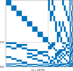
(a) $A_{\operatorname{grad}}$, standard

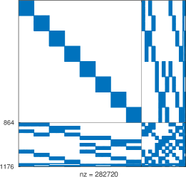
(b) $A_{\operatorname{curl}}$, standard

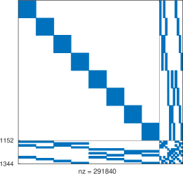
(c) $A_{\operatorname{div}}$, standard

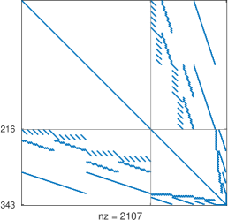
(d) $A_{\operatorname{grad}}$, FDM

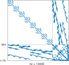
(e) $A_{\operatorname{curl}}$, FDM

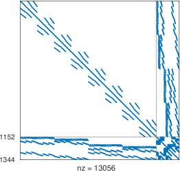
(f) $A_{\operatorname{div}}$, FDM

Figure 1: Sparsity patterns for the $2\times 2\times 2$ Pavarino–Arnold–Falk–Winther patch problem around a vertex ($p=4$), for (a, d) (1.1) (b, e) (1.2) (c, f) (1.3). The top row (a)-(c) uses standard (GLL/GL) elements, while the bottom row (d)-(f) uses the FDM variants we propose.

The second main component is to ensure optimal fill-in in the factorization of the patch problems. The Cholesky factorizations of the matrices shown in Figure 1(d-f) are sparse, even sparser than the Cholesky factorization of a low-order discretization on a grid with the same number of DOFs. However, this still incurs suboptimal setup and storage costs of $\mathcal{O}(p^{2d})$ and $\mathcal{O}(p^{d+1})$, respectively. We overcome this through the choice of Hiptmair space decompositions, which require smaller patch solves around edges and faces, and through the careful use of incomplete factorizations of vertex patch problems. Choosing edge patches in $H(\operatorname{curl})$ and face patches in $H(\operatorname{div})$ (along with patches for scalar and vector potential fields, respectively) results in patch factors with fill-in of optimal space complexity of $\mathcal{O}(p^{d})$. However, this does not address the case of $H(\operatorname{grad})$. A natural strategy is to employ incomplete Cholesky (ICC) factorizations. The zero-fill-in ICC factorization does not work: the factorization may fail, and even when it is computed it may not offer an effective relaxation. Instead, we use a nested dissection ordering and impose the sparsity pattern associated with static condensation (i.e., when the interior DOFs are eliminated). Computational experiments indicate that this still offers an excellent relaxation, while achieving optimality in both flops and storage, albeit without a theoretical basis.

The third main component is the use of auxiliary operators. The patch matrices assembled with the FDM elements are not sparse for distorted cells and/or spatially-varying $\alpha$ or $\beta$. To overcome this, we apply our preconditioner to an auxiliary operator which is constructed so that the patch matrices are sparse. The auxiliary operator employed in this work is different to that in our previous work [8] for solving (1.1): in this work, we construct the auxiliary operator by taking diagonal approximations of mass matrices involved in the definition of the stiffness matrices. The implementation of this auxiliary operator is more convenient for $H(\operatorname{curl})$ and $H(\operatorname{div})$. The quality of this approximation depends on the mesh distortion and the degree of any spatial variation in coefficients. Computational experiments suggest a slow growth of the equivalence constants with respect to $p$, but this growth is not fast enough to affect optimality of the solver.

With these components we achieve optimal complexity solvers. To illustrate this, we show in Figure 2 the number of flops and bytes required to solve the Riesz maps (1.1)–(1.3) with conjugate gradients (CG) and $\alpha=\beta=1$ on an unstructured hexahedral mesh. The setup is described in more detail in Section 5.1.

(a) Flop count, $H(\operatorname{grad})$

(b) Peak memory, $H(\operatorname{grad})$

(c) Nonzeros, $H(\operatorname{grad})$

(d) Flop count, $H(\operatorname{curl})$

(e) Peak memory, $H(\operatorname{curl})$

(f) Nonzeros, $H(\operatorname{curl})$

(g) Flop count, $H(\operatorname{div})$

(h) Peak memory, $H(\operatorname{div})$

(i) Nonzeros, $H(\operatorname{div})$

Figure 2: Flop counts, peak memory usage, and nonzeros in the sparse matrices and patch factors in the solution of the Riesz maps on an unstructured mesh with 27 cells.

For patch matrices assembled in the GLL basis (and hence with dense blocks) and factorized, the time complexity is $\mathcal{O}(p^{9})$, and the space complexity is $\mathcal{O}(p^{6})$, as expected. When assembled in the FDM basis in a sparse matrix format, the time complexity is reduced to approximately $\mathcal{O}(p^{5})$ (the empirical slope between $p=23$ and $p=31$ is $\mathcal{O}(p^{5.22})$ in Fig. 2(a)), and the space complexity is $\mathcal{O}(p^{4})$ in Fig. 2(c). The peak memory used, as shown in Fig. 2(b), is not yet scaling as $\mathcal{O}(p^{4})$, indicating that the sparse Cholesky factors are not yet the dominant term in memory. These complexities are further reduced when the FDM elements are combined with ICC factorizations: the time complexity becomes $\mathcal{O}(p^{4})$ and the space complexity $\mathcal{O}(p^{3})$, as desired.

A fourth, optional ingredient is the use of static condensation on the sparse auxiliary operator, eliminating the interior DOFs to yield patch problems posed only on the interfaces between cells. As shown in Figure 2, the time and space complexities remain $\mathcal{O}(p^{4})$ and $\mathcal{O}(p^{3})$, respectively, but there are several advantages nevertheless. First, the peak memory required is substantially reduced, by a factor of $2.5\times$–$5.3\times$ for $p=31$ , thus enabling the use of modern HPC hardware with limited RAM available per core. This reduction is caused by the fact that the patch matrices have fewer DOFs. Second, the volume of data shared between processes is reduced, to the same order as that required by operator application. This reduces parallel communication. These advantages result in a substantially faster solver.

1.1 Related work

The fast diagonalization method (FDM) [35] is a matrix factorization that enables the direct solution of problems such as (1.1) in optimal complexity, whenever separation of variables is applicable (i.e., only on certain domains and for certain coefficients $\alpha,\beta$). The FDM breaks down the $d$-dimensional problem into a sequence of one-dimensional generalized eigenvalue problems. Our construction of finite elements with orthogonality properties below in Section 2 was inspired by the FDM.

Hientzsch [18, 19] studied the extension of the FDM to the $H(\operatorname{curl})$ Riesz map (1.2). The algorithm relies on the elimination of one vector component. The reduced system for the remaining vector component can be solved directly with the FDM. With this approach, one has to solve one generalized eigenvalue problem for every cell of the mesh, whereas in the $H(\operatorname{grad})$ case (1.1) one solves a single generalized eigenvalue problem on the reference cell. Unfortunately, this strategy does not extend well to the case with three vector components, as the nested Schur complement is no longer a sum of three Kronecker products.

Low-order-refined (LOR) preconditioners [40, 12] are well known to be spectrally equivalent [9] to discrete high-order operators in $H(\operatorname{grad})$. For problems in $H(\operatorname{curl})$ and $H(\operatorname{div})$, LOR preconditioners have been studied in [13, 44]. The auxiliary low-order problem is sparse, but even for the $H(\operatorname{grad})$ case (1.1), devising efficient relaxations is challenging [43]. This is because the low-order-refined grid is anisotropic, and pointwise smoothers on the auxiliary low-order problem become ineffective as $p$ increases. To overcome this, Pazner [43] applies patchwise multigrid with ICC relaxations to (1.1), relying on a good ordering of the DOFs. This method has not been studied for (1.2) or (1.3), to the best of our knowledge. Instead, Pazner, Kolev & Dohrmann apply the AMS and ADS algebraic multigrid solvers of Hypre [15, 30, 31] to the auxiliary low-order problem, which implement the strategy proposed by Hiptmair & Xu [22]. These LOR approaches do not naturally combine with static condensation, since the density of the Schur complement arising from the elimination of DOFs that are interior to the original grid counteracts the sparsity offered by the low-order problem.

In common with the work of Schöberl & Zaglmayr [49, 53], we obtain basis functions with local complete sequence properties, i.e., on the interior of each cell the discrete spaces form a subcomplex of the de Rham complex. Our construction of the basis functions for $\mathrm{NCE}_{p}$, $\mathrm{NCF}_{p}$, and $\mathrm{DQ}_{p}$ from that of $\mathrm{Q}_{p}$ is the same, but we start from a different basis for $\mathrm{Q}_{p}$; Schöberl & Zaglmayr start with integrated Legendre polynomials on the reference interval, whereas we employ the FDM element proposed in our previous work [8]. This choice yields greater sparsity, because the mass matrix on the reference interval decouples the interior DOFs.

2 Sparsity-promoting discretization

Our goal is to construct finite elements so that the discretizations of (1.1)–(1.3) are sparse even at high $p$. Specifically, we desire that the number of nonzeros in the stiffness matrix is of the same order as its number of rows or columns, in certain cases (Cartesian cells and cellwise-constant coefficients).

2.1 Exterior calculus notation and weak formulation

To unify the discussion of (1.1)–(1.3), we adopt the language of the finite element exterior calculus (FEEC) [2]. We recognize functions in $H(\operatorname{grad})$, $H(\operatorname{curl})$, $H(\operatorname{div})$, and $L^{2}$ as differential $k$-forms for $k=0,1,2,3$, respectively, writing $H(\operatorname{d}^{k},\Omega)=H\Lambda^{k}(\Omega)$, with the exterior derivative $\operatorname{d}^{k}$ corresponding to $\operatorname{d}^{0}=\operatorname{grad}$, $\operatorname{d}^{1}=\operatorname{curl}$, $\operatorname{d}^{2}=\operatorname{div}$, $\operatorname{d}^{3}=\operatorname{null}$ (the zero map). We define the spaces

(2.1) $$V^{k}\coloneqq\{v\in H\Lambda^{k}(\Omega):\operatorname{tr}v=0\mbox{\leavevmode\nobreak\ on\leavevmode\nobreak\ }\Gamma_{D}\},$$

where the trace operator on $\partial\Omega$ is $\operatorname{tr}v=v|_{\partial\Omega}$ for $0$-forms, $\operatorname{tr}v=(v\times\mathbf{n})|_{\partial\Omega}$ for $1$-forms, $\operatorname{tr}v=(v\cdot\mathbf{n})|_{\partial\Omega}$ for $2$-forms, and $\operatorname{tr}v=0$ for $3$-forms [2], where $\mathbf{n}$ denotes the outward-facing unit normal on $\partial\Omega$. In FEEC notation, the discrete spaces on the bottom row of (1.7) are denoted as $\mathrm{Q}^{-}_{p}\Lambda^{k}(\mathcal{T}_{h})$. We denote the discrete spaces employed as $V^{k}_{h,p}\coloneqq\mathrm{Q}^{-}_{p}\Lambda^{k}(\mathcal{T}_{h})\cap V^{k}$.

With this notation, the common weak formulation of (1.1)–(1.3) is to find $u\in V^{k}$ such that

(2.2) $$a^{k}(v,u)\coloneqq(v,\beta u)_{\Omega}+(\operatorname{d}^{k}v,\alpha\operatorname{d}^{k}u)_{\Omega}=F(v)\text{ for all }v\in V^{k},$$

for $k\in\{0,1,2\}$, and where $(\cdot,\cdot)_{\Omega}$ denotes the $L^{2}(\Omega)$-inner product. The discretization we consider is to find $u_{h}\in V^{k}_{h,p}$ such that

(2.3) $$a^{k}(v_{h},u_{h})=F(v_{h})\text{ for all }v_{h}\in V^{k}_{h,p}.$$

2.2 Orthogonal basis for $H(\operatorname{grad})$ on the interval

In [8] the authors introduced a new finite element for $V^{0}_{h,p}$ on the reference interval $\hat{\mathcal{I}}\coloneqq[-1,1]$, which induces basis functions that are orthogonal in both the $L^{2}(\hat{\mathcal{I}})$- and $H(\operatorname{grad},\hat{\mathcal{I}})$-inner products. The basis functions can then be extended to tensor-product cells in arbitrary dimensions by tensor-products. We summarize the construction of [8] here. The essential idea is to solve the one-dimensional generalized eigenproblem: find $\{\hat{s}_{i}\}_{i=1}^{p-1}\subset\mathrm{P}_{p}(\hat{\mathcal{I}})$ such that

(2.4) $$(\hat{s}_{i},\hat{s}_{j})_{\hat{\mathcal{I}}}=\delta_{ij},\quad(\hat{s}^{\prime}_{i},\hat{s}^{\prime}_{j})_{\hat{\mathcal{I}}}=\lambda_{i}\delta_{ij},\quad\hat{s}_{i}(-1)=\hat{s}_{i}(1)=0,\quad i,j\in 1:(p-1),$$

where $\mathrm{P}_{p}(\hat{\mathcal{I}})$ is the set of polynomials of degree $p$ on $\hat{\mathcal{I}}$, $a:b\coloneqq[a,b]\cap\mathbb{Z}$, and where summation is not implied. This generalized eigenproblem (2.4) is solved once for a given $p$, offline. With these functions, we define the degrees of freedom $\{\hat{s}^{*}_{i}\}_{i=0}^{p}$ as

(2.5) $$\hat{s}^{*}_{i}(v)\coloneqq\begin{cases}v(-1),&i=0,\\ (\hat{s}_{i},v)_{\hat{\mathcal{I}}},&i\in 1:(p-1),\\ v(1),&i=p.\end{cases}$$

The Ciarlet triple [11] for our element is $(\hat{\mathcal{I}},\mathrm{P}_{p}(\hat{\mathcal{I}}),\{\hat{s}^{*}_{i}\}_{i=0}^{p})$. The point evaluations at the vertices guarantee $C^{0}(\hat{\mathcal{I}})$ continuity, and hence $H(\operatorname{grad},\hat{\mathcal{I}})$-conformity.

The finite element induces a reference nodal basis dual to $\{\hat{s}^{*}_{i}\}_{i=0}^{p}$ in the usual way [7, eq. (3.1.2)]. The basis functions associated with $i\in 1:(p-1)$ are the generalized eigenfunctions $\hat{s}_{i}$, by construction (cf. (2.4)). It remains to determine the interface basis functions $\hat{s}_{0},\hat{s}_{p}$. These two functions are defined via the duality condition $\hat{s}^{*}_{i}(\hat{s}_{j})=\delta_{ij}$, which reads

(2.6) $$\begin{bmatrix}\hat{s}_{0}(-1)&\hat{s}_{j}(-1)&\hat{s}_{p}(-1)\\ (\hat{s}_{i},\hat{s}_{0})_{\hat{\mathcal{I}}}&(\hat{s}_{i},\hat{s}_{j})_{\hat{\mathcal{I}}}&(\hat{s}_{i},\hat{s}_{p})_{\hat{\mathcal{I}}}\\ \hat{s}_{0}(1)&\hat{s}_{j}(1)&\hat{s}_{p}(1)\end{bmatrix}=\begin{bmatrix}1&0&0\\ 0&\delta_{ij}&0\\ 0&0&1\end{bmatrix},\quad i,j\in 1:(p-1).$$

As a direct consequence, the reference mass matrix $\hat{B}_{ij}=(\hat{s}_{i},\hat{s}_{j})_{\hat{\mathcal{I}}}$ for $i,j\in 0:p$ will become almost diagonal, with the only nonzero off-diagonal entries being $\hat{B}_{0p}=\hat{B}_{p0}$. This is crucial for maintaining sparsity in higher dimensions, as the stiffness matrix on Cartesian cells in higher dimensions is the Kronecker product of reference mass and stiffness matrices.

We obtain $\{\hat{s}_{j}\}$ numerically via Lagrange interpolants. We denote by $\hat{S}\in\mathbb{R}^{(p+1)\times(p+1)}$ the tabulation of the basis functions onto the GLL points, i.e. $\hat{S}_{ij}=\hat{s}_{j}(\hat{\xi}_{i})$, such that $\hat{s}_{j}=\ell_{i}\hat{S}_{ij}$, where $\{\ell_{j}\}$ are the Lagrange polynomials associated with the GLL points $\{\hat{\xi}_{i}\}_{i=0}^{p}$. The matrix of coefficients $\hat{S}$ is determined as follows. Denote the interface DOFs by $\Gamma\coloneqq\{0,p\}$, and the interior DOFs by $I\coloneqq 1:(p-1)$. From the first and last rows of (2.6) we deduce that $\hat{S}_{\Gamma I}=0$ and $\hat{S}_{\Gamma\Gamma}={\mathbb{I}}$, with ${\mathbb{I}}$ the identity matrix. To determine the tabulation of the interior basis functions onto $\{\hat{\xi_{i}}\}_{i\in I}$, we note that (2.4) is equivalent to the generalized eigenvalue problem: find $\hat{S}_{II}\in\mathbb{R}^{(p-1)\times(p-1)}$ and $\{\lambda_{j}\}_{j\in I}$ such that

(2.7) $$\hat{S}_{II}^{\top}\hat{A}^{\mathrm{GLL}}_{II}\hat{S}_{II}=\Lambda_{II},\quad\hat{S}_{II}^{\top}\hat{B}^{\mathrm{GLL}}_{II}\hat{S}_{II}={\mathbb{I}}.$$

Here $[\hat{A}^{\mathrm{GLL}}]_{ij}=(\ell^{\prime}_{i},\ell^{\prime}_{j})_{\hat{\mathcal{I}}}$, $[\hat{B}^{\mathrm{GLL}}]_{ij}=(\ell_{i},\ell_{j})_{\hat{\mathcal{I}}}$ are the stiffness and mass matrices discretized in the GLL basis, and $\Lambda_{II}=\operatorname{diag}(\lambda_{1},\ldots,\lambda_{p-1})$ is the diagonal matrix of eigenvalues. We solve this problem numerically with the LAPACK routine dsygv [1], which uses a Cholesky factorization of $\hat{B}^{\mathrm{GLL}}_{II}$ and the QR algorithm on a standard eigenvalue problem.

To determine $\hat{S}_{I\Gamma}$, we employ the duality condition $(\hat{s}_{i},\hat{s}_{j})_{\hat{\mathcal{I}}}=0$ for $i\in I,j\in\Gamma$ to obtain

(2.8) $$\hat{S}_{II}^{\top}(\hat{B}^{\mathrm{GLL}}_{II}\hat{S}_{I\Gamma}+\hat{B}^{\mathrm{GLL}}_{I\Gamma}\hat{S}_{\Gamma\Gamma})=0.$$

Using (2.7) and $\hat{S}_{\Gamma\Gamma}={\mathbb{I}}$, we obtain

(2.9) $$\hat{S}_{I\Gamma}=-\hat{S}_{II}\hat{S}_{II}^{\top}\hat{B}^{\mathrm{GLL}}_{I\Gamma}.$$

With this element for $V^{0}_{h,p}$, discretizations of (1.1) on Cartesian cells (axis-aligned hexahedra) are sparse, as sparse as a low-order discretization, with a sparser Cholesky factorization. Because of (2.4), the interior block of the stiffness matrix on such a Cartesian cell is diagonal.

In the next subsections, we build upon the results of [8] to construct interior-orthogonal bases for $V^{k}_{h,p}$, $k\in 1:3$.

2.3 Orthogonal basis for $L^{2}$ on the interval

We first define a basis $\{\hat{r}_{j}\}_{j=0}^{p-1}$ for the space of discontinuous polynomials of degree $p-1$ on the interval, $\mathrm{DP}_{p-1}(\hat{\mathcal{I}})$, by exploiting the fact that $\operatorname{d}(\mathrm{P}_{p})=\mathrm{DP}_{p-1}$ (where $\operatorname{d}$ is the one-dimensional derivative operator). We define the basis for $\mathrm{DP}_{p-1}(\hat{\mathcal{I}})$ as the derivatives of the interior basis functions for $\mathrm{P}_{p}$ defined above, $\{\hat{s}^{\prime}_{j}\}_{j\in I}$, augmented with the constant function:

(2.10) $$\hat{r}_{j}\coloneqq\begin{cases}\lambda_{0}^{-1/2}&j=0,\\ \lambda_{j}^{-1/2}\hat{s}^{\prime}_{j}&j=1,\ldots p-1.\end{cases}$$

Here $\lambda_{0}\coloneqq|\hat{\mathcal{I}}|$, and $\lambda_{j}\coloneqq(\hat{s}^{\prime}_{j},\hat{s}^{\prime}_{j})_{\hat{\mathcal{I}}}$ for $j\in I$ are required to normalize the basis. By construction, the set $\{\hat{s}^{\prime}_{j}\}_{j\in I}$ is orthogonal in the $L^{2}(\hat{\mathcal{I}})$-inner product. In addition $(\hat{r}_{0},\hat{r}_{j})_{\hat{\mathcal{I}}}=0$ for $j\in I$, which follows from the fact that the interior basis functions $\{\hat{s}_{j}\}_{j\in I}$ vanish at the endpoints of $\hat{\mathcal{I}}$:

(2.11) $$(\hat{r}_{0},\hat{r}_{j})_{\hat{\mathcal{I}}}=(\lambda_{0}\lambda_{j})^{-1/2}\int_{\hat{\mathcal{I}}}\hat{s}^{\prime}_{j}\,{\operatorname{d}}\hat{x}=(\lambda_{0}\lambda_{j})^{-1/2}\left(\hat{s}_{j}(1)-\hat{s}_{j}(-1)\right)=0.$$

This dependence of the basis of $\mathrm{DP}_{p-1}$ on that of $\mathrm{P}_{p}$ becomes useful in higher dimensions for enforcing interior-orthogonality in $H(\operatorname{curl})$ and $H(\operatorname{div})$. Figure 3 shows the FDM basis functions for $\mathrm{P}_{p}$ and $\mathrm{DP}_{p-1}$ and the nonzero structure of the one-dimensional differentiation matrix $\hat{D}\in\mathbb{R}^{p\times(p+1)}$ that interpolates the derivatives of $\mathrm{P}_{p}$ onto $\mathrm{DP}_{p-1}$ in the FDM bases.

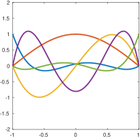
(a) $\mathrm{P}_{4}(\mathrm{FDM})$, $\hat{s}_{j}(\hat{x})$

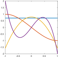
(b) $\mathrm{DP}_{3}(\mathrm{FDM})$, $\hat{r}_{j}(\hat{x})$

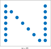
(c) $\hat{D}_{ij}=(\hat{r}_{i},\hat{s}^{\prime}_{j})_{\hat{\mathcal{I}}}$, $p=7$

Figure 3: Plots of the FDM basis functions for $p=4$ on the reference interval $\hat{\mathcal{I}}$.

2.4 Orthogonal bases for the de Rham complex

With bases for $\mathrm{P}_{p}(\hat{\mathcal{I}})$ and $\mathrm{DP}_{p-1}(\hat{\mathcal{I}})$, we construct the basis functions for $V^{k}_{h,p}(\hat{K})$, $k\in 0:3$, on the reference hexahedron $\hat{K}\coloneqq\hat{\mathcal{I}}^{3}$ in the usual tensor-product fashion [39, 3]:

(2.12) $$V^{0}_{h,p}(\hat{K})=\mathrm{Q}_{p}(\hat{K}) =\mathrm{P}_{p}(\hat{\mathcal{I}})\otimes\mathrm{P}_{p}(\hat{\mathcal{I}})\otimes\mathrm{P}_{p}(\hat{\mathcal{I}}),$$

(2.13) $$V^{1}_{h,p}(\hat{K})=\mathrm{NCE}_{p}(\hat{K}) =\begin{bmatrix}\mathrm{DP}_{p-1}(\hat{\mathcal{I}})\otimes\mathrm{P}_{p}(\hat{\mathcal{I}})\otimes\mathrm{P}_{p}(\hat{\mathcal{I}})\\ \mathrm{P}_{p}(\hat{\mathcal{I}})\otimes\mathrm{DP}_{p-1}(\hat{\mathcal{I}})\otimes\mathrm{P}_{p}(\hat{\mathcal{I}})\\ \mathrm{P}_{p}(\hat{\mathcal{I}})\otimes\mathrm{P}_{p}(\hat{\mathcal{I}})\otimes\mathrm{DP}_{p-1}(\hat{\mathcal{I}})\end{bmatrix},$$

(2.14) $$V^{2}_{h,p}(\hat{K})=\mathrm{NCF}_{p}(\hat{K}) =\begin{bmatrix}\mathrm{P}_{p}(\hat{\mathcal{I}})\otimes\mathrm{DP}_{p-1}(\hat{\mathcal{I}})\otimes\mathrm{DP}_{p-1}(\hat{\mathcal{I}})\\ \mathrm{DP}_{p-1}(\hat{\mathcal{I}})\otimes\mathrm{P}_{p}(\hat{\mathcal{I}})\otimes\mathrm{DP}_{p-1}(\hat{\mathcal{I}})\\ \mathrm{DP}_{p-1}(\hat{\mathcal{I}})\otimes\mathrm{DP}_{p-1}(\hat{\mathcal{I}})\otimes\mathrm{P}_{p}(\hat{\mathcal{I}})\end{bmatrix},$$

(2.15) $$V^{3}_{h,p}(\hat{K})=\mathrm{DQ}_{p-1}(\hat{K}) =\mathrm{DP}_{p-1}(\hat{\mathcal{I}})\otimes\mathrm{DP}_{p-1}(\hat{\mathcal{I}})\otimes\mathrm{DP}_{p-1}(\hat{\mathcal{I}}).$$

We introduce tensor-product bases for each finite element space in (1.7). For $\mathrm{Q}_{p}(\hat{K})$ we define $\{\hat{\psi}_{ijl}\}$ as

(2.16) $$\hat{\psi}_{ijl}\coloneqq\hat{s}_{i}(\hat{x}_{1})\hat{s}_{j}(\hat{x}_{2})\hat{s}_{l}(\hat{x}_{3}),\quad(i,j,l)\in(0:p)^{3}.$$

For $\mathrm{NCE}_{p}(\hat{K})$ we define $\{\hat{\Psi}^{(m)}_{ijl}\}$ as

(2.17) $$\hat{\Psi}^{(1)}_{ijl} \coloneqq\hat{r}_{i}(\hat{x}_{1})\hat{s}_{j}(\hat{x}_{2})\hat{s}_{l}(\hat{x}_{3})\mathbf{e}_{1},\quad(i,j,l)\in(0:p-1)\times(0:p)\times(0:p),$$

$$\hat{\Psi}^{(2)}_{ijl} \coloneqq\hat{s}_{i}(\hat{x}_{1})\hat{r}_{j}(\hat{x}_{2})\hat{s}_{l}(\hat{x}_{3})\mathbf{e}_{2},\quad(i,j,l)\in(0:p)\times(0:p-1)\times(0:p),$$

$$\hat{\Psi}^{(3)}_{ijl} \coloneqq\hat{s}_{i}(\hat{x}_{1})\hat{s}_{j}(\hat{x}_{2})\hat{r}_{l}(\hat{x}_{3})\mathbf{e}_{3},\quad(i,j,l)\in(0:p)\times(0:p)\times(0:p-1).$$

For $\mathrm{NCF}_{p}(\hat{K})$ we define $\{\hat{\Phi}^{(m)}_{ijl}\}$ as

(2.18) $$\hat{\Phi}^{(1)}_{ijl} \coloneqq\hat{s}_{i}(\hat{x}_{1})\hat{r}_{j}(\hat{x}_{2})\hat{r}_{l}(\hat{x}_{3})\mathbf{e}_{1},\quad(i,j,l)\in(0:p)\times(0:p-1)\times(0:p-1),$$

$$\hat{\Phi}^{(2)}_{ijl} \coloneqq\hat{r}_{i}(\hat{x}_{1})\hat{s}_{j}(\hat{x}_{2})\hat{r}_{l}(\hat{x}_{3})\mathbf{e}_{2},\quad(i,j,l)\in(0:p-1)\times(0:p)\times(0:p-1),$$

$$\hat{\Phi}^{(3)}_{ijl} \coloneqq\hat{r}_{i}(\hat{x}_{1})\hat{r}_{j}(\hat{x}_{2})\hat{s}_{l}(\hat{x}_{3})\mathbf{e}_{3},\quad(i,j,l)\in(0:p-1)\times(0:p-1)\times(0:p).$$

For $\mathrm{DQ}_{p-1}(\hat{K})$ we define $\{\hat{\phi}_{ijl}\}$ as

(2.19) $$\hat{\phi}_{ijl}\coloneqq\hat{r}_{i}(\hat{x}_{1})\hat{r}_{j}(\hat{x}_{2})\hat{r}_{l}(\hat{x}_{3}),\quad(i,j,l)\in(0:p-1)^{3}.$$

By construction, the interior basis functions of these four bases are orthonormal in the $L^{2}(\hat{K})$-inner product. Moreover, each horizontal arrow in (1.7) gives rise to the following relations between the interior basis functions, where $(i,j,l)\in(1:p-1)^{3}$:

(2.20) $$\operatorname{grad}\hat{\psi}_{ijl}=\lambda_{i}^{1/2}\hat{\Psi}_{ijl}^{(1)}+\lambda_{j}^{1/2}\hat{\Psi}_{ijl}^{(2)}+\lambda_{l}^{1/2}\hat{\Psi}_{ijl}^{(3)},$$

(2.21) $$\operatorname{curl}\hat{\Psi}_{ijl}^{(1)} =\lambda_{j}^{1/2}\hat{\Phi}_{ijl}^{(3)}-\lambda_{l}^{1/2}\hat{\Phi}_{ijl}^{(2)},$$

$$\operatorname{curl}\hat{\Psi}_{ijl}^{(2)} =\lambda_{l}^{1/2}\hat{\Phi}_{ijl}^{(1)}-\lambda_{i}^{1/2}\hat{\Phi}_{ijl}^{(3)},$$

$$\operatorname{curl}\hat{\Psi}_{ijl}^{(3)} =\lambda_{i}^{1/2}\hat{\Phi}_{ijl}^{(2)}-\lambda_{j}^{1/2}\hat{\Phi}_{ijl}^{(1)},$$

(2.22) $$\operatorname{div}\hat{\Phi}_{ijl}^{(1)}=\lambda_{i}^{1/2}\hat{\phi}_{ijl},\quad\operatorname{div}\hat{\Phi}_{ijl}^{(2)}=\lambda_{j}^{1/2}\hat{\phi}_{ijl},\quad\operatorname{div}\hat{\Phi}_{ijl}^{(3)}=\lambda_{l}^{1/2}\hat{\phi}_{ijl}.$$

Therefore, the FDM bases form a local complete sequence at the interior DOF level, i.e., for a fixed $(i,j,l)\in(1:p-1)^{3}$ we can establish a subcomplex of the discrete de Rham complex on the reference cube

(2.23) $$\leavevmode\hbox to304.25pt{\vbox to55.49pt{\text{[drawing]}}}. {\mathrm{Q}_{p}(\hat{K})} {\mathrm{NCE}_{p}(\hat{K})} {\mathrm{NCF}_{p}(\hat{K})} {\mathrm{DQ}_{p-1}(\hat{K})} {\operatorname{span}\{\hat{\psi}_{ijl}\}} {\operatorname{span}\{\hat{\Psi}^{(m)}_{ijl}\}_{m=1}^{3}} {\operatorname{span}\{\hat{\Phi}^{(m)}_{ijl}\}_{m=1}^{3}} {\operatorname{span}\{\hat{\phi}_{ijl}\}} \scriptstyle{\operatorname{grad}} \scriptstyle{\operatorname{curl}} \scriptstyle{\operatorname{div}} \scriptstyle{\operatorname{grad}} \scriptstyle{\operatorname{curl}} \scriptstyle{\operatorname{div}} {\mathrm{Q}_{p}(\hat{K})} {\mathrm{NCE}_{p}(\hat{K})} {\mathrm{NCF}_{p}(\hat{K})} {\mathrm{DQ}_{p-1}(\hat{K})} {\operatorname{span}\{\hat{\psi}_{ijl}\}} {\operatorname{span}\{\hat{\Psi}^{(m)}_{ijl}\}_{m=1}^{3}} {\operatorname{span}\{\hat{\Phi}^{(m)}_{ijl}\}_{m=1}^{3}} {\operatorname{span}\{\hat{\phi}_{ijl}\}} \scriptstyle{\operatorname{grad}} \scriptstyle{\operatorname{curl}} \scriptstyle{\operatorname{div}} \scriptstyle{\operatorname{grad}} \scriptstyle{\operatorname{curl}} \scriptstyle{\operatorname{div}}$$

Taking into account the $L^{2}(\hat{K})$-orthogonality of the interior basis functions, (2.23) implies that on Cartesian cells, the sparsity pattern of the stiffness matrices $A^{k}$ discretizing the bilinear form for the Riesz map $a^{k}(\cdot,\cdot)$ in (2.2) connects each interior DOF only to interior DOFs that share $(i,j,l)$. Thus the interior block of $A^{k}$ has at most $d$ nonzeros per row (for $k\in\{1,2\}$) or one nonzero per row (for $k\in\{0,3\}$), as depicted in Figure 1.

3 Auxiliary sparse preconditioning

The orthogonality on the reference cell, and the subsequent sparsity of the mass and stiffness matrices, will only carry over to cells that are Cartesian and when $\alpha,\beta$ are cellwise constant. In this section we construct a preconditioner that extends the sparsity we would have in the Cartesian case to the case of practical interest, with distorted cells and spatially varying coefficients. The essential idea is to build an auxiliary operator that is sparse in the FDM basis, by construction. To explain this, we must first introduce some notions of finite element assembly.

3.1 Pullbacks and finite element assembly

The discrete spaces $V^{k}_{h,p}$ are defined in such way that the trace is continuous across facets. This is achieved through the pullback $\mathcal{F}^{k}_{K}:V^{k}(\hat{K})\to V^{k}(K)$ that maps functions on the reference cell $\hat{K}$ to functions on the physical cell $K$. The discrete spaces are defined in terms of the pullback,

(3.1) $$V^{k}_{h,p}(\mathcal{T}_{h})\coloneqq\left\{v_{h}\in V^{k}:\operatorname{\forall}K\in\mathcal{T}_{h}\operatorname{\exists}\hat{v}\in V^{k}_{h,p}(\hat{K})\mbox{\leavevmode\nobreak\ s.t.\leavevmode\nobreak\ }v_{h}|_{K}=\mathcal{F}^{k}_{K}(\hat{v})\right\}.$$

The application of the pullback to a reference function can be described as the composition of the inverse of the coordinate mapping $F_{K}:\hat{K}\to K$ with multiplication by a factor depending on the Jacobian of the coordinate transformation $J_{K}\coloneqq\mathrm{D}F_{K}$. Let $u$ be a $k$-form on $K$ mapped from $\hat{u}$ in $\hat{K}$. Then

(3.2) $$u(\mathbf{x})=\mathcal{F}^{k}_{K}(\hat{u}(\hat{\mathbf{x}}))=\begin{cases}\hat{u}(F^{-1}_{K}(\mathbf{x}))&k=0,\\ J_{K}^{-\top}\hat{u}(F^{-1}_{K}(\mathbf{x}))&k=1,\\ (\det J_{K})^{-1}J_{K}\hat{u}(F^{-1}_{K}(\mathbf{x}))&k=2,\\ (\det J_{K})^{-1}\hat{u}(F^{-1}_{K}(\mathbf{x}))&k=3,\end{cases}$$

for $\mathbf{x}\in K$ mapped from $\hat{\mathbf{x}}\in\hat{K}$ via $\mathbf{x}=F_{K}(\hat{\mathbf{x}})$. The pullback preserves continuity of the traces of a $k$-form across cell facets, which is the natural continuity requirement for $\operatorname{d}^{k}$.

Another key property of the pullback is that it commutes with $\operatorname{d}^{k}$. The exterior derivative $\operatorname{d}^{k}u$ can be mapped from that of the reference value $\hat{\operatorname{d}}{}^{k}\hat{u}$,

(3.3) $$\operatorname{d}^{k}\mathcal{F}_{K}^{k}(\hat{u})=\mathcal{F}_{K}^{k+1}(\hat{\operatorname{d}}{}^{k}\hat{u}),$$

where $\hat{\operatorname{d}}$ is the exterior derivative with respect to the reference coordinates $\hat{\mathbf{x}}$. The pullback is incorporated in FEM by storing reference values as the DOFs in the vector of coefficients $\underline{u}=(\hat{u}_{1},\ldots,\hat{u}_{N})^{\top}$ representing a discrete function on a cell $K$ as

(3.4) $$u_{h}|_{K}=\sum_{j=1}^{N}\hat{u}_{j}\mathcal{F}_{K}^{k}(\hat{\psi}^{k}_{j}),$$

where $\hat{\psi}^{k}_{j}$ indexes the basis functions for $V^{k}_{h,p}(\hat{K})$ defined in (2.16)–(2.19). The assembly of a bilinear form involves the cell matrices

(3.5) $$[A^{k}_{K}]_{ij}=a^{k}(\mathcal{F}_{K}^{k}(\hat{\psi}^{k}_{i}),\mathcal{F}_{K}^{k}(\hat{\psi}^{k}_{j})).$$

3.2 Construction of sparse preconditioners

We rewrite the bilinear form $a^{k}(\cdot,\cdot)$ in terms of reference arguments and use the property (3.3), to obtain

(3.6) $$a^{k}(v_{h},u_{h})=\left(\mathcal{F}_{K}^{k}(\hat{v}),\beta\,\mathcal{F}_{K}^{k}(\hat{u})\right)_{K}+\left(\mathcal{F}_{K}^{k+1}(\hat{\operatorname{d}}{}^{k}\hat{v}),\alpha\,\mathcal{F}_{K}^{k+1}(\hat{\operatorname{d}}{}^{k}\hat{u})\right)_{K},$$

for $v_{h},u_{h}\in V^{k}_{h,p}(K)$. From (3.6) we see that the second term is an inner product of arguments in $V^{k+1}_{h,p}(K)$. This means that the cell matrices can be sum-factorized in terms of the differentiation matrix $\hat{D}$ acting on reference values, and weighted mass matrices on $V^{k}_{h,p}$ and $V^{k+1}_{h,p}$,

(3.7) $$A^{k}_{K}=M^{k}_{\beta,K}+\hat{D}^{\top}M^{k+1}_{\alpha,K}\hat{D}.$$

Intuitively, we want each of the matrices in the sum-factorization (3.7) to be sparse in order to achieve sparsity in $A^{k}_{K}$. In higher dimensions the matrix $\hat{D}$ inherits the sparsity of the one-dimensional differentiation matrix depicted in Figure 3(c). On Cartesian cells and for cellwise constant $\alpha,\beta$, the matrices $M_{\alpha,K}^{k+1},M_{\beta,K}^{k}$ are sparse, but they are not sparse when these conditions do not hold.

We consider $M^{k}_{\beta,K}$ first. As $M^{k}_{\beta,K}$ discretizes a weighted $L^{2}(K)$-inner product, we propose to assemble the matrix in terms of a broken space $\overline{V}{}^{k}_{h,p}$ with a fully $L^{2}$-orthonormal basis. In this broken space, the mass matrix to approximate will be diagonal in the Cartesian, constant-coefficient case. The basis for $\mathrm{DP}_{p-1}$ was already $L^{2}$-orthogonal; we define a new basis for $\overline{\mathrm{P}}_{p}$, the broken variant of $\mathrm{P}_{p}$, by orthogonalizing the interface basis functions with respect to each other. The interface functions were already orthogonal to the interior ones, which follows from the definition of the interior degrees of freedom (2.5) and the duality condition (2.6).

Let $\overline{M}{}^{k}_{\beta,K}$ be the weighted mass matrix in the basis for $\overline{V}{}^{k}_{h,p}(K)$. Then

(3.8) $$M^{k}_{\beta,K}=\overline{G}{}^{\top}\overline{M}{}^{k}_{\beta,K}\overline{G},$$

where $\overline{G}$ is a sparse basis transformation matrix from $V^{k}_{h,p}(\hat{K})$ to $\overline{V}{}^{k}_{h,p}(\hat{K})$. This matrix $\overline{G}$ is block-diagonal with one block per vector component, where each block is a Kronecker product of identity matrices and (sparse) basis transformation matrices from $\mathrm{P}_{p}(\hat{\mathcal{I}})$ to $\overline{\mathrm{P}}_{p}(\hat{\mathcal{I}})$. The matrix $\overline{M}{}^{k}_{\beta,K}$ is diagonal when $K$ is Cartesian and $\beta$ is constant, unlike $M^{k}_{\beta,K}$ (which is sparse, but not diagonal in this case). To obtain a sparse approximation to $M^{k}_{\beta,K}$, we simply take the diagonal of $\overline{M}{}^{k}_{\beta,K}$ in (3.8). This contrasts with taking the diagonal directly of $M^{k}_{\beta,K}$, which would alter the operator even when $K$ is Cartesian and $\beta$ is constant.

Applying the same idea to $M_{\alpha,K}^{k+1}$, we approximate the stiffness matrix $A^{k}_{K}$ with an auxiliary matrix that is sparse on any given cell, for any spatial variation of problem coefficients:

(3.9) $$A^{k}_{K}\approx P^{k}_{K}\coloneqq\overline{G}{}^{\top}\operatorname{diag}(\overline{M}{}^{k}_{\beta,K})\overline{G}+\overline{D}{}^{\top}\operatorname{diag}(\overline{M}{}^{k+1}_{\alpha,K})\overline{D},$$

where $\overline{D}\coloneqq\overline{G}\hat{D}$.

Using this auxiliary operator ensures that the patchwise problems that we solve in our multigrid relaxation are sparse. We describe these patchwise problems next.

4 Multigrid relaxation by subspace correction

4.1 Notation

We now introduce the preconditioners we use to solve (2.2). We express the solvers in terms of space decompositions [52], which we summarize briefly here. Given a discrete space $V^{k}_{h,p}$, the preconditioner is induced by a particular choice of how to write it as a sum of (smaller) function spaces:

(4.1) $$V^{k}_{h,p}=\sum_{i}V_{i}.$$

This notation for the sum of vector spaces means that for any $v_{h}\in V^{k}_{h,p}$, there exist $\{v_{i}\in V_{i}\}_{i}$ such that $v_{h}=\sum_{i}v_{i}$. The decomposition is not typically unique. Given an initial guess for the solution to a variational problem posed over $V^{k}_{h,p}$, the Galerkin projection of the equation for the error is solved over each $V_{i}$ (additively or multiplicatively). This gives an approximation to the error in each subspace $V_{i}$, which are combined. A cycle over each subspace constitutes one step of a subspace correction method. For more details, see Xu [52].

In order to describe the space decompositions we will use, we require some concepts from algebraic topology. We conceive of the mesh $\mathcal{T}_{h}$ as a regular cell complex [45, 27, 33]. This represents the mesh as a set of entities of different dimensions, with incidence relations between them. For $d=3$, the entities are vertices, edges, faces, and cells, of dimensions $k=0,1,2,3$, respectively. The incidence relations encode the boundary operator, relating an entity of dimension $k\geq 1$ to its bounding sub-entities of dimension $k-1$. For example, they encode that a cell has as its sub-entities certain faces, while a face has as its sub-entities certain edges. Let $E^{k}(\mathcal{T}_{h})$ denote the set of entities of dimension $k$ in $\mathcal{T}_{h}$. We also define $E^{-1}(\mathcal{T}_{h})\coloneqq\emptyset$ for notational convenience.

The star operation on an entity $j$ of dimension $k$, denoted $\star j$, returns the union of the interiors of all entities of dimension at least $k$ that recursively contain $j$ as a sub-entity [38, §2][14]. For example, the star of a cell is simply its interior, since there are no entities of higher dimension. The star of an internal face $\star f$ returns the patch of cells formed of the two cells that share $f$, excluding the boundary of the patch. Similarly, the star of a vertex $\star v$ returns the union of the interiors of all edges, faces, and cells sharing $v$, as well as the vertex itself; geometrically, this forms the patch of cells sharing $v$, again excluding the boundary of the patch. The stars of a vertex, edge, and face are shown in Figure 4.

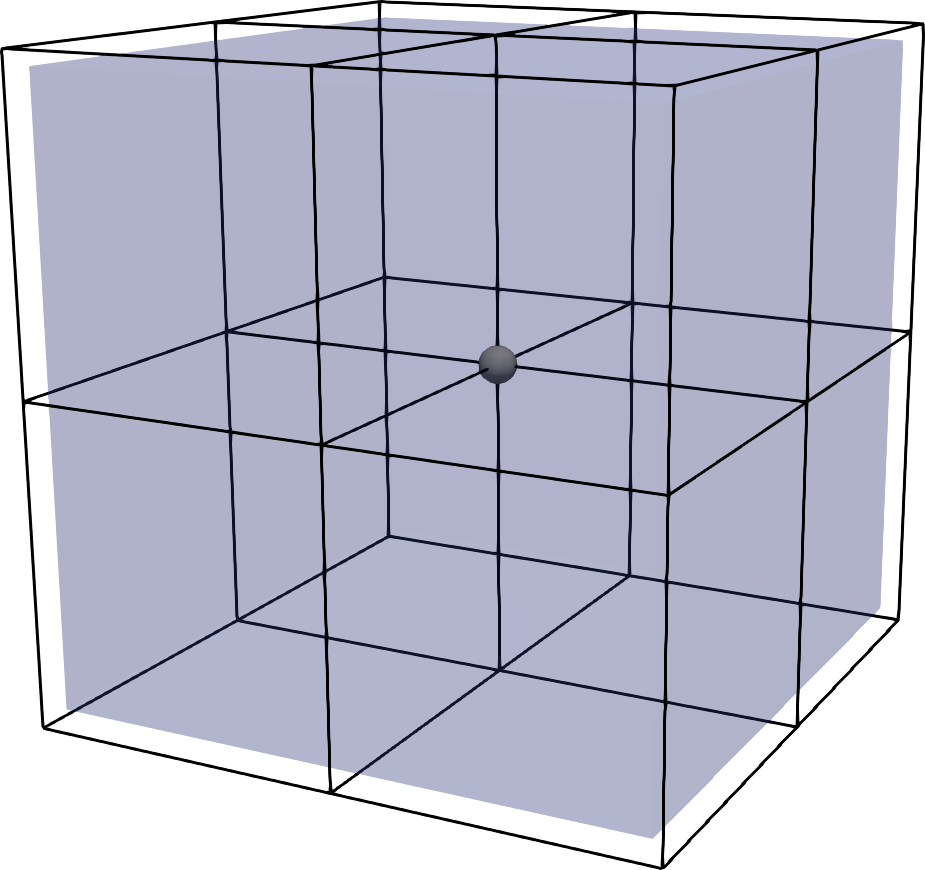
(a) vertex star

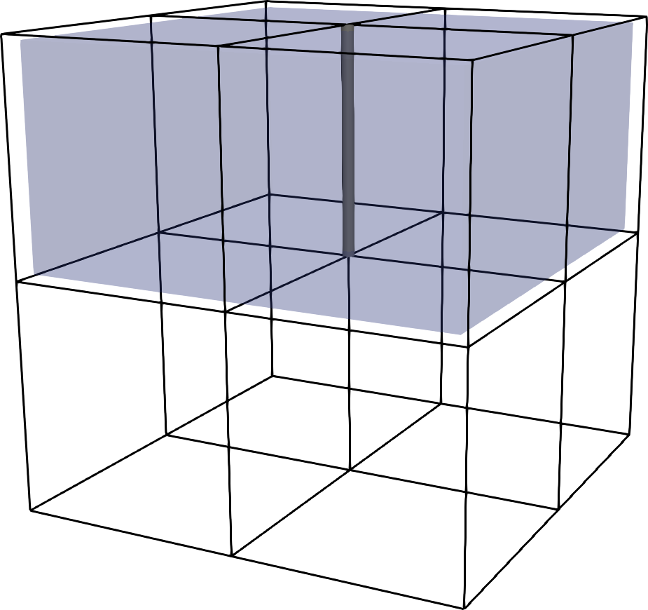
(b) edge star

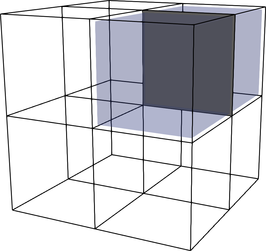
(c) face star

Figure 4: The stars of (a) a vertex (b) an edge (c) a face. Solving a discrete problem restricted to a star involves solving for all degrees of freedom contained in the star.

Given a function space $V_{h}$ and an entity $j$, we define

(4.2) $$\left.V_{h}\right|_{\star j}\coloneqq\left\{v\in V_{h}:\mathrm{support}(v)\subseteq\star j\right\}.$$

This gives a local function space around an entity upon which a variational problem may be solved. Informally, it defines a block employed in a block Jacobi method, taking all the DOFs in the patch of cells around $j$, excluding those on the boundary.

4.2 Designing space decompositions

The framework (4.1) offers a great deal of freedom in designing solvers. Since the bilinear form $a^{k}(\cdot,\cdot)$ is symmetric and coercive, powerful and general theories are available to guide the choice of space decomposition [52, 47, 32]; for a summary, see [16]. We remark on some general principles here.

First, the cost of each iteration of subspace correction will depend on the dimensions of the subspaces $\{V_{i}\}$. It is therefore desirable that the space decomposition be as fine as possible, i.e., $\mathrm{dim}(V_{i})$ be as small as possible for each $i$. If $V^{k}_{h,p}=\mathrm{span}\{\psi_{1},\dots,\psi_{J}\}$, then choosing $V_{i}\coloneqq\mathrm{span}\{\psi_{i}\}$ for $i=1,\dots,J$ gives the finest possible space decomposition. The subspace correction methods induced by this space decomposition are (point) Jacobi or Gauß–Seidel iterations. However, as with any one-level method (without a coarse space), the convergence of these schemes on their own is unacceptably slow.

To discuss the convergence of the scheme, we introduce some notation; we draw this discussion from [16]. Define the operator $\mathcal{A}^{k}:V^{k}_{h,p}\to(V^{k}_{h,p})^{*}$ associated with the bilinear form $a^{k}(\cdot,\cdot)$ via

(4.3) $$\langle v,\mathcal{A}^{k}u\rangle\coloneqq a^{k}(v,u)\text{ for all }v,u\in V^{k}_{h,p},$$

where $\langle\cdot,\cdot\rangle$ denotes the duality pairing. For each subspace we denote the inclusion operator $\mathcal{R}_{i}^{*}:V_{i}\to V^{k}_{h,p}$ and its $L^{2}$ adjoint, the restriction $\mathcal{R}_{i}:(V^{k}_{h,p})^{*}\to V_{i}^{*}$, and we define the restriction of $\mathcal{A}^{k}$ to $V_{i}$ by

(4.4) $$\langle v_{i},\mathcal{A}_{i}u_{i}\rangle=\langle\mathcal{R}_{i}^{*}v_{i},\mathcal{A}^{k}\mathcal{R}_{i}^{*}u_{i}\rangle\text{ for all }v_{i},u_{i}\in V_{i},$$

i.e., $\mathcal{A}_{i}=\mathcal{R}_{i}\mathcal{A}^{k}\mathcal{R}_{i}^{*}$. The additive subspace correction preconditioner associated with the decomposition $\{V_{i}\}$ is then given by

(4.5) $$\mathcal{P}^{-1}=\sum_{i}\mathcal{R}_{i}^{*}\mathcal{A}_{i}^{-1}\mathcal{R}_{i}.$$

Let $T=\mathcal{P}^{-1}\mathcal{A}^{k}$ be the preconditioned operator. Our goal is to estimate the condition number $\kappa(T)$ to bound the convergence of the conjugate gradient method. The condition number is bounded by two parameters.

The first, $N_{O}$, is the maximum overlap among subspaces. For each subspace $V_{i}$, consider its set of overlapping subspaces $\mathrm{overlap}(V_{i})\coloneqq\{V_{j}:\operatorname{\exists}v_{i}\in V_{i},v_{j}\in V_{j}\text{ s.t. }a(\mathcal{R}_{i}^{*}v_{i},\mathcal{R}_{j}^{*}v_{j})\neq 0\}$; $N_{O}$ is the maximum over $i$ of $|\mathrm{overlap}(V_{i})|$. This bounds the maximal eigenvalue of $T$. It is straightforward to analyze $N_{O}$ by inspection on a particular family of meshes, and $N_{O}$ is naturally independent of $h$, $p$, $\alpha$, and $\beta$. The second measures the stability of the space decomposition. Assume that there exists $c_{1}$ such that

(4.6) $$\inf_{\begin{subarray}{c}v_{i}\in V_{i}\\ \sum_{i}v_{i}=v_{h}\end{subarray}}\sum_{i}\|v_{i}\|^{2}_{\mathcal{A}_{i}}\leq c_{1}\|v_{h}\|^{2}_{\mathcal{A}}\text{ for all }v_{h}\in V^{k}_{h,p}.$$

Then the minimum eigenvalue of $T$ is bounded below by $c_{1}^{-1}$.

In order for the convergence of our solver to be robust, we require that $c_{1}$ is independent of $h$, $p$, $\alpha$, and $\beta$. For example, the slow convergence of the Jacobi iteration on the Poisson problem is because the space decomposition is not stable in the mesh parameter $h$. This may be addressed by incorporating a global coarse space (on a coarser mesh with $H>h$) into the space decomposition (as in a two-level domain decomposition method, or a multigrid method), which gives a stability constant independent of $h$ for the Poisson equation. However, this space decomposition is still not stable in $p$ for (1.1), nor is it stable in $h$, $\alpha$, $\beta$ for (1.2) or (1.3). Essentially, this is because for $k=0$, eigenfunctions associated with small eigenvalues of the operator are smooth and can be well-represented on a coarse grid, but this is not true for $k\in\{1,2\}$. Building on work by Pavarino [42], Arnold, Falk & Winther [4, 5], and Hiptmair [20], we now discuss the space decompositions proposed by Schöberl and Zaglmayr [49, 53] that are robust in $h$, $p$, $\alpha$, and $\beta$ in numerical experiments.

4.3 Choice of space decompositions

The Pavarino–Arnold–Falk–Winther (PAFW) decomposition is

(4.7) $$V^{k}_{h,p}=V^{k}_{h,1}+\sum_{v\in E^{0}(\mathcal{T}_{h})}\left.V^{k\phantom{-}}_{h,p}\right|_{\star v}.$$

This combines solving local problems on overlapping patches of cells sharing a vertex with a coarse solve at lowest order ($p=1$). The Pavarino–Hiptmair (PH) decomposition is

(4.8) $$V^{k}_{h,p}=V^{k}_{h,1}+\sum_{i\in E^{k}(\mathcal{T}_{h})}\left.V^{k\phantom{-}}_{h,p}\right|_{\star i}+\sum_{j\in E^{k-1}(\mathcal{T}_{h})}\left.\operatorname{d}^{k-1}{}V^{k-1}_{h,p}\right|_{\star j}.$$

These decompositions (4.7) and $\eqref{eq:ph}$ coincide for $k=0$. For example, for $H(\operatorname{curl})$ ($k=1$), the PH decomposition iterates over all edges $i$ of the mesh, solving patch problems on the cells sharing each edge, while $j$ iterates over all vertices. The PH decomposition involves an auxiliary problem on the local potential space $V^{k-1}_{h,p}|_{\star j}$: find $\psi\in V^{k-1}_{h,p}|_{\star j}$ such that

(4.9) $$a^{k}(\operatorname{d}^{k-1}\phi,\operatorname{d}^{k-1}\psi)=(\operatorname{d}^{k-1}\phi,\beta\operatorname{d}^{k-1}\psi)_{\star j}=L(\operatorname{d}^{k-1}\phi)\quad\text{ for all }\phi\in\left.V^{k-1}_{h,p}\right|_{\star j},$$

since $\operatorname{d}^{k}\circ\operatorname{d}^{k-1}=0$. For example, for $H(\operatorname{curl})$, this becomes: for each vertex $v$, find $\psi\in V^{0}_{h,p}|_{\star v}$ such that

$$(\operatorname{grad}\phi,\beta\operatorname{grad}\psi)_{\star v}=L(\operatorname{grad}\phi)\quad\text{ for all }\phi\in\left.V^{0}_{h,p}\right|_{\star v},$$

a local scalar-valued Poisson-type problem.

Remark 1.

In the case of $H(\operatorname{div})$ $(k=2)$, the auxiliary problem is singular, with a kernel consisting of the curl-free functions. One alternative is to define an auxiliary space with this kernel removed, i.e., posed on the space $V^{k-1}_{h,p}/\operatorname{d}^{k-2}V^{k-2}_{h,p}$. Another approach is to add a symmetric and positive-definite term on the kernel, such as $(\operatorname{div}\phi,\beta\operatorname{div}\psi)$, as done by the Hiptmair–Xu decomposition [22], but with the conforming auxiliary space $[H(\operatorname{grad})]^{d}$. Our implementation deals with this problem in a pragmatic way by simply adding a small multiple of the mass matrix for $V^{k-1}_{h,p}$ to the patch matrix.

Remark 2.

The $p$-robustness of the PAFW decomposition was proven for $k=0$ in the tensor-product case by Pavarino [42] and in the simplicial case by Schöberl et al. [48]. A similar decomposition (with geometric multigrid coarsening, not coarsening in polynomial degree) was proposed by Arnold, Falk, & Winther for $k=1$ and $k=2$ [4, 5], and proven to be robust to mesh size $h$ and variations in constant $\alpha$ and $\beta$. To the best of our knowledge the $p$-robustness of (4.7) and (4.8) have not been proven for $k=1$ or $k=2$, although numerical experiments indicate that they are $p$-robust for $p\leq 31$.

To simplify notation, we drop the superscript $k$ from the stiffness matrices $A^{k}$. The algebraic realization of the PAFW relaxation (combined additively) reads

(4.10) $$P^{-1}_{\mathrm{PAFW}}=R_{0}^{\top}A_{0}^{-1}R_{0}+\sum_{v\in E^{0}(\mathcal{T}_{h})}R_{v}^{\top}A_{v}^{-1}R_{v}.$$

Here $R_{0}$ is the restriction matrix from $(V^{k}_{h,p})^{*}$ to $(V^{k}_{h,1})^{*}$, $A_{0}$ is the stiffness matrix for the original bilinear form $a^{k}(\cdot,\cdot)$ rediscretized with the lowest-order element $(p=1)$, $R_{v}$ are Boolean restriction matrices onto the DOFs of each vertex-star patch $\star v$, and $A_{v}=R_{v}AR_{v}^{\top}$ are sub-matrices of $A$ corresponding to the rows and columns of DOFs of the patch. Furthermore, another subspace correction method such as geometric or algebraic multigrid, may be employed as the $p$-coarse solver to approximate $A_{0}^{-1}$.

Similarly, the additive PH relaxation is implemented as

(4.11) $$P^{-1}_{\mathrm{PH}}=R_{0}^{\top}A_{0}^{-1}R_{0}+\sum_{i\in E^{k}(\mathcal{T}_{h})}R_{i}^{\top}A_{i}^{-1}R_{i}+D\left(\sum_{j\in E^{k-1}(\mathcal{T}_{h})}R_{j}^{\top}B_{j}^{-1}R_{j}\right)D^{\top}.$$

where $R_{0},A_{0}$ have the same meaning as in (4.10), $D$ is the matrix tabulating the differential operator $\operatorname{d}^{k-1}:V^{k-1}_{h,p}\to V^{k}_{h,p}$, $R_{i},R_{j}$ are Boolean restriction matrices onto star patches on entities of dimension $k$ and $k-1$, respectively, $A_{i}=R_{i}AR_{i}^{\top}$ are patch matrices, and $B_{j}$ are patch matrices extracted from $B$, which is obtained as the discretization of $a^{k}(\operatorname{d}^{k-1}\phi,\operatorname{d}^{k-1}\psi)$. With the FDM basis it is feasible to compute and store the $D$ matrix, as it is sparse and applies to reference values.

4.4 Statically-condensed space decompositions

As seen from Figure 1, the minimal coupling between interior DOFs that arises from the orthogonality of the FDM elements invites the use of static condensation. Static condensation yields a finer space decomposition with smaller subspaces by eliminating the interior DOFs. The overlapping subspaces only involve interface DOFs.

The statically-condensed Pavarino–Arnold–Falk–Winther (SC-PAFW) decomposition is

(4.12) $$V^{k}_{h,p}=V^{k}_{h,1}+\left.V^{k\phantom{-}}_{h,p}\right|_{\mathcal{I}}+\sum_{v\in E^{0}(\mathcal{T}_{h})}\left.\tilde{V}^{k\phantom{-}}_{h,p}\right|_{\star v},$$

Here $\mathcal{I}\coloneqq E^{d}(\mathcal{T}_{h})$ is the set of cell interiors of $\mathcal{T}_{h}$, and $V^{k}_{h,p}|_{\mathcal{I}}\coloneqq\sum_{c\in\mathcal{I}}V^{k}_{h,p}|_{c}$ is the space of discrete functions supported on cell interiors. The cell-interior problems do not overlap with each other and can be solved independently. We denote by $\tilde{V}^{k}_{h,p}\coloneqq(V^{k}_{h,p}|_{\mathcal{I}})^{\perp}$ the space of discrete harmonic functions of $V^{k}_{h,p}$, defined as the $a^{k}(\cdot,\cdot)$-orthogonal complement of $V^{k}_{h,p}|_{\mathcal{I}}$,

(4.13) $$\tilde{V}^{k}_{h,p}=\left\{\tilde{v}\in V^{k}_{h,p}:\,a^{k}(w,\tilde{v})=0\operatorname{\forall}w\in\left.V^{k}_{h,p}\right|_{\mathcal{I}}\right\}.$$

By definition $V^{k}_{h,p}=V^{k}_{h,p}|_{\mathcal{I}}\oplus\tilde{V}^{k}_{h,p}$; this orthogonality leads to reduced overlap of the star patches, compared to the non-statically-condensed case.

The statically-condensed Pavarino–Hiptmair (SC-PH) decomposition is

(4.14) $$V^{k}_{h,p}=V^{k}_{h,1}+\left.V^{k\phantom{-}}_{h,p}\right|_{\mathcal{I}}+\sum_{i\in E^{k}(\mathcal{T}_{h})}\left.\tilde{V}^{k\phantom{-}}_{h,p}\right|_{\star i}+\sum_{j\in E^{k-1}(\mathcal{T}_{h})}\left.\operatorname{d}^{k-1}\tilde{V}^{k-1}_{h,p}\right|_{\star j}.$$

These decompositions again coincide for $k=0$.

Denote by $I,\Gamma$ the sets of interior and interface (vertex, edge, and face) DOFs, respectively. Reordering the DOFs of $A$ yields a $2\times 2$ block matrix, with inverse obtained from its block $LDL^{\top}$ decomposition

(4.15) $$\begin{bmatrix}A_{II}&A_{I\Gamma}\\ A_{\Gamma I}&A_{\Gamma\Gamma}\end{bmatrix}^{-1}=\begin{bmatrix}{\mathbb{I}}&-A_{II}^{-1}A_{I\Gamma}\\ 0&{\mathbb{I}}\end{bmatrix}\begin{bmatrix}A^{-1}_{II}&0\\ 0&S^{-1}\end{bmatrix}\begin{bmatrix}{\mathbb{I}}&0\\ -A_{\Gamma I}A_{II}^{-1}&{\mathbb{I}}\end{bmatrix},$$

where $S$ denotes the interface Schur complement

(4.16) $$S=A_{\Gamma\Gamma}-A_{\Gamma I}A_{II}^{-1}A_{I\Gamma}.$$

When solvers for $A_{II}$ and $S$ are available, the application of $A^{-1}$ times a residual vector can be performed with a single application of $S^{-1}$ and only two applications of $A_{II}^{-1}$. This is because the second and third instances of $A_{II}^{-1}$ in the RHS of (4.15) act on the same interior DOFs of the incoming residual vector.

Another way to write (4.15) gives rise to the additive interpretation of the harmonic subspace correction step

(4.17) $$A^{-1}=R_{I}^{\top}A_{II}^{-1}R_{I}+R_{\Gamma}^{\top}S^{-1}R_{\Gamma},$$

where $R_{I}$ is a Boolean restriction onto the interior DOFs, and

(4.18) $$R_{\Gamma}=\begin{bmatrix}-A_{\Gamma I}A_{II}^{-1}&{\mathbb{I}}\end{bmatrix}$$

is the ideal restriction operator onto the discrete harmonic subspace. $R_{\Gamma}^{\top}$ maps vectors of coefficients in $\tilde{V}^{k}_{h,p}$ to $V^{k}_{h,p}$. The orthogonality between $\tilde{V}^{k}_{h,p}$ and $V^{k}_{h,p}|_{\mathcal{I}}$ is reflected by the identity $R_{\Gamma}AR_{I}^{\top}=0$.

Remark 3.

For Cartesian cells, in $H(\operatorname{grad})$ $(k=0)$, the interior DOFs are fully decoupled and $A_{II}$ is diagonal, while for $k=1,2$, the cell-interior problems only couple at most $d$ DOFs, as shown in (2.23). There exists a reordering of the interior DOFs for which $A_{II}$ becomes block diagonal with diagonal blocks of dimension at most $d\times d$, implying that $A_{II}$ shares its sparsity pattern with its inverse. Therefore $A_{II}$ coincides with its zero-fill-in incomplete Cholesky factorization. Hence we may assemble and store the Schur complement $S$, even for very high $p$. This also holds for the auxiliary sparse operator in Section 3 on general cells, as it inherits the sparsity pattern of the Cartesian case by construction.

Remark 4.

We choose to use a Krylov method on $A$, as opposed to implementing one on the condensed system involving $S$. The action of the true $A_{II}^{-1}$ involves the iterative solution of local problems on cell-interiors, inducing $\mathcal{O}(p^{d+1})$ computational cost in the application of the true $S$. Although the sum-factorized application of the true $A_{\Gamma\Gamma},A_{I\Gamma},A_{\Gamma I}$ only involves $\mathcal{O}(p^{d})$ flops, and the conditioning of the preconditioned operator is generally better, this results in a longer runtime when compared to using a Krylov method on $A$ with the statically-condensed preconditioner built from the sparse auxiliary operator, especially for the case $k=1$.

The algebraic realization of the SC-PAFW relaxation (4.12) approximates the Schur complement in (4.17) with

(4.19) $$S^{-1}\approx S^{-1}_{\mathrm{PAFW}}\coloneqq\tilde{R}_{0}^{\top}A_{0}^{-1}\tilde{R}_{0}+\sum_{v\in E^{0}(\mathcal{T}_{h})}{\tilde{R}_{v}}^{\top}S_{v}^{-1}\tilde{R}_{v},$$

where $\tilde{R}_{0}$ is the restriction matrix from $(\tilde{V}^{k}_{h,p})^{*}$ to $({V}^{k}_{h,1})^{*}$, and $\tilde{R}_{v}$ are the Boolean restriction matrices onto the interface DOFs of the vertex-star patch $\star v$, and $S_{v}=\tilde{R}_{v}S\tilde{R}_{v}^{\top}$.

Similarly, the SC-PH relaxation (4.14) is implemented as

(4.20) $$S^{-1}_{\mathrm{PH}}\coloneqq\tilde{R}_{0}^{\top}A_{0}^{-1}\tilde{R}_{0}+\sum_{i\in E^{k}(\mathcal{T}_{h})}{\tilde{R}_{i}}^{\top}S_{i}^{-1}\tilde{R}_{i}+\tilde{D}\left(\sum_{j\in E^{k-1}(\mathcal{T}_{h})}{\tilde{R}_{j}}^{\top}\tilde{B}_{j}^{-1}\tilde{R}_{j}\right)\tilde{D}^{\top},$$

where $\tilde{R}_{0},A_{0}$ have the same meaning as in (4.19), $\tilde{D}=D_{\Gamma\Gamma}$ is the matrix tabulating the differential operator $\operatorname{d}^{k-1}:\tilde{V}^{k-1}_{h,p}\to\tilde{V}^{k}_{h,p}$, $\tilde{R}_{i},\tilde{R}_{j}$ are Boolean restriction matrices onto the interface DOFs of star patches on entities of dimension $k$ and $k-1$, respectively, $S_{i}=\tilde{R}_{i}S\tilde{R}_{i}^{\top}$ are patch matrices, and $\tilde{B}_{j}$ are patch matrices extracted from the interface Schur complement of the discretization of $a^{k}(\operatorname{d}^{k-1}\phi,\operatorname{d}^{k-1}\psi)$.

4.5 Achieving optimal fill-in

To achieve optimal complexity of our solver, we require that the factorizations of the patch matrices arising in the space decomposition be optimal in storage. The number of nonzeros in the factorizations also relates to the number of flops required to compute them. For the PAFW space decomposition (4.7), in Figure 5(a-c) we observe fill-in of $\mathcal{O}(p^{4})$ nonzeros in the Cholesky factorization of the vertex patch problems in $H(\operatorname{grad})$, $H(\operatorname{curl})$, and $H(\operatorname{div})$, even with a nested dissection ordering. Moreover, computing this factorization incurs $\mathcal{O}(p^{6})$ flops. These costs compare unfavorably with the $\mathcal{O}(p^{3})$ storage and $\mathcal{O}(p^{4})$ flops required by sum-factorized operator application.

To overcome this, for $H(\operatorname{grad})$ we employ an incomplete Cholesky factorization. Incomplete Cholesky factorization with zero fill-in (ICC(0), depicted in blue in Figure 5(a) and (d)) does not yield an effective relaxation method, even when it can be computed. In contrast, the incomplete Cholesky factorization on the statically-condensed sparsity pattern does yield an effective relaxation. This factorization has $\mathcal{O}(p^{3})$ fill-in ($\mathcal{O}(p)$ nonzeros on $\mathcal{O}(p^{2})$ rows). It appears that this sparsity pattern (depicted in green in Figure 5(d)) offers a suitable intermediate between the zero-fill-in pattern and the full Cholesky factorization (depicted in red in Figure 5(a)).

For $H(\operatorname{curl})$ and $H(\operatorname{div})$, the PH (4.8) space decomposition is finer than PAFW: it requires the solution of smaller vector-valued subproblems, in the stars of edges or faces, instead of in the stars of vertices (cf. Figure 4). For the edge-star problems solved for $H(\operatorname{curl})$, in Figure 5(e) we apply a reverse Cuthill–McKee reordering and observe that the matrix is block-diagonal with $p$ sparse blocks of size $\mathcal{O}(p)\times\mathcal{O}(p)$. Hence the Cholesky factorization for the PH patch has optimal storage without requiring the use of incomplete factorizations, assuming fill-in in the entire block. On the auxiliary scalar-valued problem posed on the vertex star, we employ the incomplete Cholesky factorization described above. For the face-star problems solved in $H(\operatorname{div})$, there is no coupling at all between the face degrees of freedom in the FDM basis, and ICC(0) offers a direct solver (Figure 5(f)). In fact, the SC-PH relaxation for $H(\operatorname{div})$ is equivalent to point-Jacobi applied to the interface Schur complement.

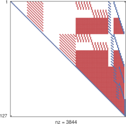
(a) $\mathrm{chol}(A^{0})$, $\mathrm{Q}_{4}(\star v)$

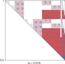
(b) $\mathrm{chol}(A^{1})$, $\mathrm{NCE}_{4}(\star v)$

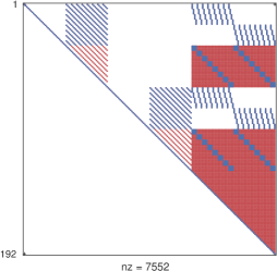
(c) $\mathrm{chol}(A^{2}$), $\mathrm{NCF}_{4}(\star v)$

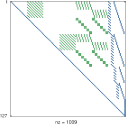
(d) $\mathrm{ICC}(A^{0})$, $\mathrm{Q}_{4}(\star v)$

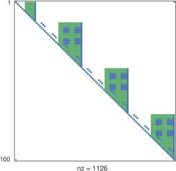
(e) $\mathrm{chol}(A^{1})$, $\mathrm{NCE}_{4}(\star e)$

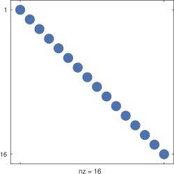
(f) $\mathrm{chol}(A^{2})$, $\mathrm{NCF}_{4}(\star f)$

Figure 5: The interface-interface block of the patch problems arising in the PAFW (a-c) and the PH (d-f) space decompositions on a regular Cartesian mesh with FDM elements. Here $\star v$, $\star e$, $\star f$ correspond to the vertex, edge, and face stars depicted in Figure 4. The sparsity pattern of the problem posed in the FDM basis is coloured in blue. The additional nonzeros required by the Cholesky factorization are colored in red or green, depending on whether they require suboptimal storage (as in (a-c)) or optimal storage (as in (e-f)). In (d) we plot the sparsity pattern of the interface Schur complement arising in static condensation, which offers a sparsity pattern intermediate between the zero fill-in and the full Cholesky factorization.

5 Numerical experiments

We provide an implementation of the $\mathrm{P}_{p}$ and $\mathrm{DP}_{p-1}$ elements with the FDM basis functions on the interval in FIAT [25]. The extension to quadrilaterals and hexahedra is achieved by taking tensor-products of the one-dimensional elements with FInAT [23]. Code for the sum-factorized evaluation of the residual is automatically generated by Firedrake [17, 24], implementing a Gauß–Lobatto quadrature rule with $3(p+1)/2$ points along each direction. The sparse preconditioner discretizing the auxiliary operator is implemented as a PETSc [6] preconditioner as firedrake.FDMPC.

The preconditioners described in Section 4 have been presented as additive. However, the preconditioners in our experiments are implemented as hybrid multigrid/Schwarz methods [34]: they combine patches additively within each level, and the levels are combined multiplicatively in a V(1,1)-cycle. The Cholesky factorization of the patch matrices is computed using CHOLMOD [10] and the ICC factorization is done with PETSc’s own implementation. Most of our computations were performed on a single node of the ARCHER2 system, with two 64-core AMD EPYC 7742 CPUs (2.25 GHz) and 512 GiB of RAM.

Code for all examples has been archived and is available at [54].

5.1 Riesz maps: robust iteration counts and optimal complexity

We first present numerical evidence demonstrating that our preconditioner for the weighted Riesz maps (1.1)–(1.3) yields CG iteration counts that are robust to mesh size $h$, polynomial degree $p$, and the coefficients $\alpha$ and $\beta$. For concreteness, in Figure 6 we present a solver diagram for the $H(\operatorname{curl})$ problem (1.2) with the SC-PH relaxation and geometric multigrid with Hiptmair–Jacobi relaxation [20] on the $p$-coarse space; the solver diagrams for the other Riesz maps and space decompositions are analogous.

Figure 6: Solver diagram for the $H(\operatorname{curl})$ Riesz map using static condensation and incomplete Cholesky factorization on vertex patches (SC-PH/FDM/ICC).

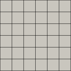
(a) Cartesian

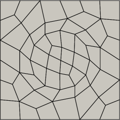
(b) unstructured

Figure 7: The meshes employed in Section 5.1 are the extrusions with six cells in the vertical of the two-dimensional meshes shown here.

We consider two mesh hierarchies of $\Omega=(0,1)^{3}$, one structured and one unstructured. The coarse meshes are the extrusions with six cells in the vertical of the two-dimensional meshes depicted in Figure 7. We then uniformly refine these $l\geq 0$ times. Each run is terminated when the (natural) $P^{-1}$-norm of the residual is reduced by a factor of $10^{8}$ starting from a zero initial guess. Each problem has homogeneous Dirichlet boundary conditions on $\Gamma_{D}=\partial\Omega$ and a randomized right-hand side that is prescribed independently of $\alpha,\beta$, through its Riesz representative

(5.1) $$F(v)=(v,w_{h,p}^{k})_{\Omega}+(\operatorname{d}^{k}v,\operatorname{d}^{k}w_{h,p}^{k})_{\Omega},\quad\mbox{for\leavevmode\nobreak\ }w_{h,p}^{k}\in V^{k}_{h,p}.$$

We first consider the robustness of our solvers with respect to mesh refinement $l$ and polynomial degree $p$, in Tables 1–3. In these experiments we fix $\alpha=1$ and $\beta=10^{-8}$. The mesh with distorted cells is useful to measure the effect of the diagonal approximation in the sparse auxiliary operator (3.9), since the Jacobian of a non-affine coordinate mapping gives rise to variable coefficients in the reference coordinates, recall (3.6). The results show almost complete $p$- and $h$-robustness in the Cartesian case, and very slow growth of iteration counts in the unstructured case.

We next consider the robustness with respect to $\alpha$ and $\beta$ for fixed $p=7$, $l=2$, for the $H(\operatorname{curl})$ and $H(\operatorname{div})$ problems (1.2)–(1.3), in Tables 4–5. Again, iteration counts do not vary substantially as the coefficients are varied, indicating the desired parameter-robustness. As expected, we observe that the iteration counts only depend on the ratio $\alpha/\beta$, which shows that our solver is invariant to a rescaling of the system matrix.

We next record the flop counts, peak memory usage, and matrix nonzeros for the PH and SC-PH solvers (with either Cholesky or ICC for the $H(\operatorname{grad})$ vertex-star patches) while varying $p$ with $\alpha=\beta=1$ with the mesh shown in Figure 8. This smaller mesh was used so that we could solve the problem at higher $p$ using the GLL basis. The results were reported above in Section 1, Figure 2.

Table 1: CG iteration counts for the $H(\operatorname{grad})$ Riesz map solved with the $\{$chol/SC-chol; ICC/SC-ICC$\}$ preconditioners. Empty table cells indicate an unsuccessful termination due to memory limitations.

	Cartesian						Unstructured
$p\setminus l$	0		1		2		0		1		2
1	1/1	1/1	8/8	8/8	8/8	8/8	1/1	1/1	12/12	12/12	14/14	14/14
3	14/11	14/11	15/11	15/11	15/11	15/11	18/18	18/18	18/19	18/19	18/21	18/21
7	12/9	13/10	12/9	13/10	12/9	13/10	19/21	20/21	19/23	20/23	19/24	20/24
11	11/9	12/10	11/9	12/10	–/9	–/10	20/23	22/24	19/24	22/24	–/–	–/25
15	10/8	13/11	10/8	13/11			21/24	24/25	20/25	23/25

Table 2: CG iteration counts for the $H(\operatorname{curl})$ Riesz map solved with the $\{$PAFW/SC-PAFW; PH/SC-PH$\}$ preconditioners.

	Cartesian						Unstructured
$p\setminus l$	0		1		2		0		1		2
1	2/2	2/2	13/13	11/11	14/14	12/12	2/2	2/2	18/18	16/16	20/20	19/19
3	14/11	20/14	15/12	22/16	15/12	22/16	18/20	26/23	19/22	27/24	19/23	27/25
7	13/10	20/15	14/11	21/16	14/11	21/16	21/23	33/29	21/25	32/28	21/25	32/28
11	13/10	20/15	14/11	21/16			23/25	36/31	22/26	34/30
15	13/10	20/16	14/12	21/17			24/26	37/32	–/–	–/31

Table 3: CG iteration counts for the $H(\operatorname{div})$ Riesz map solved with the $\{$PAFW/SC-PAFW; PH/SC-PH$\}$ preconditioners.

	Cartesian						Unstructured
$p\setminus l$	0		1		2		0		1		2
1	2/2	2/2	11/11	14/14	12/12	15/15	2/2	2/2	17/17	22/22	19/19	22/22
3	9/8	15/11	9/8	16/13	10/9	16/13	15/21	24/22	16/23	25/25	18/25	26/27
7	9/7	17/13	9/8	17/13	9/9	17/14	18/25	31/27	18/26	30/28	19/27	30/29
11	9/7	17/13	9/8	18/14			19/27	33/29	19/28	31/29
15	9/8	17/13	9/8	18/14			19/28	34/30	–/28	–/30

Table 4: CG iteration counts for the $H(\operatorname{curl})$ Riesz map discretized with $p=7$, $l=2$ solved using the $\{$PAFW/SC-PAFW; PH/SC-PH$\}$ hybrid preconditioners. For the table cell marked –, the PH patch matrix is numerically singular.

	Cartesian						Unstructured
$\beta\setminus\alpha$	$10^{-3}$		$10^{0}$		$10^{3}$		$10^{-3}$		$10^{0}$		$10^{3}$
$10^{-6}$	12/9	20/15	14/11	22/16	16/24	22/18	19/27	31/28	21/27	32/28	20/25	–/32
$10^{-3}$	10/8	18/14	12/9	20/15	14/11	22/16	17/27	30/28	19/27	31/28	21/27	32/28
$10^{0}$	12/10	20/15	10/8	18/14	12/9	20/15	19/27	31/28	17/27	30/28	19/27	31/28
$10^{3}$	11/8	21/13	12/10	20/15	10/8	18/14	24/28	42/32	19/27	31/28	17/27	30/28
$10^{6}$	11/8	23/14	11/8	21/13	12/9	20/15	29/30	51/38	24/28	42/32	19/27	31/28

Table 5: CG iteration counts for the $H(\operatorname{div})$ Riesz map discretized with $p=7$, $l=2$ solved using the $\{$PAFW/SC-PAFW; PH/SC-PH$\}$ hybrid preconditioners.

	Cartesian						Unstructured
$\beta\setminus\alpha$	$10^{-3}$		$10^{0}$		$10^{3}$		$10^{-3}$		$10^{0}$		$10^{3}$
$10^{-6}$	8/8	15/11	9/9	17/14	10/11	17/15	16/23	26/25	19/27	30/29	19/27	30/29
$10^{-3}$	6/6	12/9	8/8	15/11	9/9	17/14	12/18	20/19	16/23	26/25	19/27	30/29
$10^{0}$	8/7	15/11	6/6	12/9	8/8	15/11	16/22	26/23	12/18	20/19	16/23	26/25
$10^{3}$	7/5	21/11	8/7	15/11	6/6	12/9	18/28	38/28	16/22	26/23	12/18	20/19
$10^{6}$	7/4	23/10	7/5	21/11	8/7	15/11	22/31	48/33	18/28	38/28	16/22	26/23

Figure 8: The mesh employed for the complexity plots in Figure 2 is the extrusion with three cells in the vertical of the two-dimensional meshes shown here.

5.2 Piecewise-constant coefficients

As a test case for our $H(\operatorname{curl})$ multigrid solver, we consider a definite Maxwell problem proposed by Kolev & Vassilevski [30, §6.2] and adapted by Pazner et al. [44, §6.4]. The problem models electromagnetic diffusion in an annular copper wire in air, with a piecewise-constant diffusion coefficient $\beta$ in (1.2). As in Pazner et al., we employ a $\mathrm{Q}_{3}$ coordinate field. We set $\Gamma_{D}=\emptyset$, $\alpha=1$, $\beta_{\text{copper}}=1$, and vary the diffusion constant of air $\beta_{\text{air}}$. Since the SC-PH relaxation exhibits the best performance in the experiments of Section 5.1, we only consider this solver here, and as the $p$-coarse solver we apply a single Hypre AMS [30] algebraic multigrid cycle. For the Krylov solver, we set a relative tolerance of $10^{-8}$.

We first consider robustness of CG iteration counts to the magnitude of the jump in the coefficients, in Table 6. The results exhibit almost perfect robustness across twelve orders of magnitude for $\beta_{\text{air}}$ and across polynomial degrees between 2 and 14. This contrasts with [44, Table 2], where the iteration counts for the LOR-AMS solver roughly double from $p=2$ to $p=6$. We also tabulate the memory and solve times required as a function of $p$ in Table 7 for fixed $\beta_{\text{air}}=10^{-6}$.

Table 6: CG iteration counts for the $H(\operatorname{curl})$ definite Maxwell problem with piecewise-constant coefficients, solved with the SC-PH preconditioner.

		$\beta_{\text{air}}$
$p$	#DOFs	$10^{-6}$	$10^{-3}$	$10^{0}$	$10^{3}$	$10^{6}$
2	516,820	25	23	21	29	33
3	1,731,408	24	22	21	26	31
4	4,088,888	25	23	21	25	31
5	7,968,340	26	24	21	28	30
6	13,748,844	27	24	21	26	29
10	63,462,980	28	25	21	27	29
14	173,920,348	28	25	22	28	25

Table 7: Memory usage and runtimes for the definite Maxwell problem in $H(\operatorname{curl})$ with piecewise-constant coefficients ($\beta_{\text{air}}=10^{-6}$) solved with the SC-PH preconditioner. NNZ Mat includes the number of nonzeros of the symmetric part of $H(\operatorname{curl})$ and $H(\operatorname{grad})$ Schur complements, the ideal restriction matrix onto the interface of $H(\operatorname{curl})$, and the tabulation of the gradient of the interface basis functions. Memory records the storage of all matrices across the solver. The runtime has been broken down into assembly of the sparse Schur complements, setup of the subspace problems, and solve times.

$p$	NNZ Mat	NNZ Fact	Memory (GB)	Assembly (s)	Setup (s)	Solve (s)
2	$1.7318\text{\times}{10}^{07}$	$1.4738\text{\times}{10}^{07}$	$1.03$	$0.42$	$1.31$	$1.11$
3	$5.3952\text{\times}{10}^{07}$	$6.5279\text{\times}{10}^{07}$	$2.53$	$0.59$	$1.58$	$1.46$
4	$1.2503\text{\times}{10}^{08}$	$1.7344\text{\times}{10}^{08}$	$5.45$	$0.90$	$3.47$	$2.73$
5	$2.4192\text{\times}{10}^{08}$	$3.6076\text{\times}{10}^{08}$	$10.22$	$1.42$	$6.46$	$4.48$
6	$4.16\text{\times}{10}^{08}$	$6.4875\text{\times}{10}^{08}$	$17.28$	$2.22$	$8.49$	$7.64$
10	$1.9117\text{\times}{10}^{09}$	$3.2381\text{\times}{10}^{09}$	$76.04$	$9.60$	$31.67$	$34.15$
14	$5.2321\text{\times}{10}^{09}$	$9.1607\text{\times}{10}^{09}$	$209.86$	$27.08$	$75.10$	$94.90$

5.3 Mixed formulation of Hodge Laplacians

The Riesz maps provide building blocks for developing preconditioners for more complex systems [21, 26, 37, 36]. In this final example, we demonstrate this by constructing preconditioners for the mixed formulation of the Hodge Laplacians associated with the $L^{2}$ de Rham complex. For $\Gamma_{D}=\emptyset$, the problem is to find $(\sigma,u)\in V^{k-1}\times V^{k}$ such that

(5.2) $$-(\tau,\sigma)_{\Omega}+(\operatorname{d}^{k-1}\tau,u)_{\Omega} =0 \quad\forall\,\tau\in V^{k-1},$$

(5.3) $$(v,\operatorname{d}^{k-1}\sigma)_{\Omega}+(\operatorname{d}^{k}v,\operatorname{d}^{k}u)_{\Omega} =F(v) \quad\forall\,v\in V^{k},$$

where $F(v)$ is a random right-hand side given by (5.1). For $k=3$, the Hodge Laplacian problem corresponds to a mixed formulation of the Poisson equation.

To solve this saddle point problem, we follow the operator preconditioning framework of Hiptmair and Mardal & Winther [21, 37], employing a block-diagonal preconditioner with the Riesz maps ($\alpha=\beta=1$) for $V^{k-1}$ and $V^{k}$. We use 4 Chebyshev iterations preconditioned by the SC-PH solver for each block. For $L^{2}$, we use 4 Chebyshev iterations preconditioned by point-Jacobi in the FDM basis for $\mathrm{DQ}_{p-1}$. As outer Krylov solver we employ the minimum residual method (MINRES) [41], as this allows for the solution of indefinite problems using a symmetric coercive preconditioner. The convergence criterion for the iteration is a relative reduction of the (natural) $P^{-1}$-norm of the residual by a factor of $10^{8}$, starting from a zero initial guess. The iteration counts for the cases $k=1,2,3$ are reported in Table 8. As for the Riesz maps, we observe robustness with respect to both $h$ and $p$. The 4 inner Chebyshev iterations ensure that the preconditioner for each block is properly scaled, and for these problems, the MINRES iteration counts are typically reduced by a factor greater than 4 when compared to those obtained with a single V-cycle on each block.

Table 8: MINRES iteration counts for the mixed formulation of the Hodge Laplacians $(k=1,2,3)$ preconditioned with the Riesz maps using 4 Chebyshev iterations of the SC-PH solvers on each block.

	$H(\operatorname{grad})\times H(\operatorname{curl})$						$H(\operatorname{curl})\times H(\operatorname{div})$						$H(\operatorname{div})\times L^{2}$
	Cartesian			Unstructured			Cartesian			Unstructured			Cartesian			Unstructured
$p\setminus l$	0	1	2	0	1	2	0	1	2	0	1	2	0	1	2	0	1	2
3	9	9	9	16	16	17	8	7	7	15	16	18	8	8	8	12	14	14
7	9	9	8	20	19	19	8	8	6	19	18	18	8	8	8	14	14	13
11	9	9		23	21		8	8		20	18		8	8		15	14
15	9	9		23	21		8	6		20	18		8	8		15	14

6 Conclusion

We have developed multigrid solvers for the Riesz maps associated with the $L^{2}$ de Rham complex whose space and time complexities in polynomial degree are the same as that required for operator application. Numerical experiments demonstrate that the solvers are robust to mesh refinement, polynomial degree, and problem coefficients, and that they remain effective on unstructured grids. However, the solvers are not robust with respect to anisotropy, in common with other methods [28]. The approach relies on developing new finite elements with desirable interior-orthogonality properties, auxiliary operators that are sparse by construction, the careful use of incomplete factorizations, and the choice of space decomposition. The resulting solvers can be employed in the operator preconditioning framework to develop preconditioners for more complex problems with solution variables in $H(\operatorname{grad})$, $H(\operatorname{curl})$, and $H(\operatorname{div})$.

References

- [1] E. Anderson, Z. Bai, C. Bischof, S. Blackford, J. Demmel, J. Dongarra, J. Du Croz, A. Greenbaum, S. Hammarling, A. McKenney, and D. Sorensen, LAPACK Users’ Guide, SIAM, Philadelphia, PA, third ed., 1999.
- [2] D. N. Arnold, Finite Element Exterior Calculus, SIAM, 2018.
- [3] D. N. Arnold, D. Boffi, and F. Bonizzoni, Finite element differential forms on curvilinear cubic meshes and their approximation properties, Numer. Math., 129 (2015), pp. 1–20.
- [4] D. N. Arnold, R. Falk, and R. Winther, Preconditioning in and applications, Math. Comput., 66 (1997), pp. 957–984.
- [5] D. N. Arnold, R. S. Falk, and R. Winther, Multigrid in and , Numer. Math., 85 (2000), pp. 197–217.
- [6] S. Balay, S. Abhyankar, M. F. Adams, S. Benson, J. Brown, P. Brune, K. Buschelman, E. Constantinescu, L. Dalcin, A. Dener, V. Eijkhout, J. Faibussowitsch, W. D. Gropp, V. Hapla, T. Isaac, P. Jolivet, D. Karpeev, D. Kaushik, M. G. Knepley, F. Kong, S. Kruger, D. A. May, L. C. McInnes, R. T. Mills, L. Mitchell, T. Munson, J. E. Roman, K. Rupp, P. Sanan, J. Sarich, B. F. Smith, S. Zampini, H. Zhang, H. Zhang, and J. Zhang, PETSc/TAO users manual, Tech. Report ANL-21/39 - Revision 3.19, Argonne National Laboratory, 2023.
- [7] S. C. Brenner and L. R. Scott, The Mathematical Theory of Finite Element Methods, vol. 15 of Texts in Applied Mathematics, Springer-Verlag New York, third ed., 2008.
- [8] P. D. Brubeck and P. E. Farrell, A scalable and robust vertex-star relaxation for high-order FEM, SIAM J. Sci. Comput., 44 (2022), pp. A2991–A3017.
- [9] C. Canuto, P. Gervasio, and A. Quarteroni, Finite-element preconditioning of G-NI spectral methods, SIAM J. Sci. Comput., 31 (2010), pp. 4422–4451.
- [10] Y. Chen, T. A. Davis, W. W. Hager, and S. Rajamanickam, Algorithm 887: CHOLMOD, Supernodal Sparse Cholesky Factorization and Update/Downdate, ACM Trans. Math. Softw., 35 (2008).
- [11] P. G. Ciarlet, The finite element method for elliptic problems, SIAM, 2002.
- [12] M. O. Deville and E. H. Mund, Finite-element preconditioning for pseudospectral solutions of elliptic problems, SIAM J. Sci. Stat. Comput., 11 (1990), pp. 311–342.
- [13] C. R. Dohrmann, Spectral Equivalence of Low-Order Discretizations for High-Order and Spaces, SIAM J. Sci. Comput., 43 (2021), pp. A3992–A4014.
- [14] O. Egorova, M. Savchenko, V. Savchenko, and I. Hagiwara, Topology and geometry of hexahedral complex: combined approach for hexahedral meshing, J. Comput. Sci. Technol., 3 (2009), pp. 171–182.
- [15] R. D. Falgout and U. M. Yang, Hypre: A Library of High Performance Preconditioners, in Computational Science – ICCS 2002, P. M. A. Sloot, A. G. Hoekstra, C. J. K. Tan, and J. J. Dongarra, eds., vol. 2331 of Lecture Notes in Computer Science, Springer Berlin Heidelberg, 2002, pp. 632–641.
- [16] P. E. Farrell, M. G. Knepley, L. Mitchell, and F. Wechsung, PCPATCH: software for the topological construction of multigrid relaxation methods, ACM Trans. Math. Softw., 47 (2021).
- [17] D. A. Ham, P. H. J. Kelly, L. Mitchell, C. J. Cotter, R. C. Kirby, K. Sagiyama, N. Bouziani, S. Vorderwuelbecke, T. J. Gregory, J. Betteridge, D. R. Shapero, R. W. Nixon-Hill, C. J. Ward, P. E. Farrell, P. D. Brubeck, I. Marsden, T. H. Gibson, M. Homolya, T. Sun, A. T. T. McRae, F. Luporini, A. Gregory, M. Lange, S. W. Funke, F. Rathgeber, G.-T. Bercea, and G. R. Markall, Firedrake user manual, (2023).
- [18] B. Hientzsch, Fast solvers and domain decomposition preconditioners for spectral element discretizations of problems in , PhD thesis, New York University, 2001.
- [19] B. Hientzsch, Domain decomposition preconditioners for spectral Nédélec elements in two and three dimensions, in Domain Decomposition Methods in Science and Engineering, Springer, 2005, pp. 597–604.
- [20] R. Hiptmair, Multigrid Method for Maxwell’s Equations, SIAM J. Numer. Anal., 36 (1998), pp. 204–225.
- [21] R. Hiptmair, Operator preconditioning, Comput. Math. Appl., 52 (2006), pp. 699–706.
- [22] R. Hiptmair and J. Xu, Nodal auxiliary space preconditioning in and spaces, SIAM J. Numer. Anal., 45 (2007), pp. 2483–2509.
- [23] M. Homolya, R. C. Kirby, and D. A. Ham, Exposing and exploiting structure: optimal code generation for high-order finite element methods, 2017, https://arxiv.org/abs/1711.02473.
- [24] M. Homolya, L. Mitchell, F. Luporini, and D. A. Ham, TSFC: a structure-preserving form compiler, SIAM J. Sci. Comput., 40 (2018), pp. C401–C428.
- [25] R. C. Kirby, Algorithm 839: FIAT, a new paradigm for computing finite element basis functions, ACM Trans. Math. Soft., 30 (2004), pp. 502–516.
- [26] R. C. Kirby, From functional analysis to iterative methods, SIAM Rev., 52 (2010), pp. 269–293.
- [27] M. G. Knepley and D. A. Karpeev, Mesh algorithms for PDE with Sieve I: Mesh distribution, Sci. Program., 17 (2009), pp. 215–230.
- [28] T. Kolev et al., High-order algorithmic developments and optimizations for large-scale GPU-accelerated simulations, Tech. Report CEED-MS36, Lawrence Livermore National Laboratory, Livermore, CA, 2021.
- [29] T. Kolev, P. Fischer, M. Min, J. Dongarra, J. Brown, V. Dobrev, T. Warburton, S. Tomov, M. S. Shephard, A. Abdelfattah, et al., Efficient exascale discretizations: High-order finite element methods, Int. J. High Perform. Comput. Appl., 35 (2021), pp. 527–552.
- [30] T. V. Kolev and P. S. Vassilevski, Parallel auxiliary space AMG for problems, J. Comput. Math., 27 (2009), pp. 604–623.
- [31] T. V. Kolev and P. S. Vassilevski, Parallel auxiliary space AMG solver for problems, SIAM J. Sci. Comput., 34 (2012), pp. A3079–A3098.
- [32] Y.-J. Lee, J. Wu, J. Xu, and L. Zikatanov, Robust subspace correction methods for nearly singular systems, Math. Models Methods Appl. Sci., 17 (2007), pp. 1937–1963.
- [33] A. Logg, Efficient representation of computational meshes, Int. J. Comput. Sci. Eng., 4 (2009), pp. 283–295.
- [34] J. W. Lottes and P. F. Fischer, Hybrid multigrid/Schwarz algorithms for the spectral element method, J. Sci. Comput., 24 (2005), pp. 45–78.
- [35] R. E. Lynch, J. R. Rice, and D. H. Thomas, Direct solution of partial difference equations by tensor product methods, Numer. Math., 6 (1964), pp. 185–199.
- [36] J. Málek and Z. Strakoš, Preconditioning and the Conjugate Gradient Method in the Context of Solving PDEs, vol. 1 of SIAM Spotlights, SIAM, 2014.
- [37] K.-A. Mardal and R. Winther, Preconditioning discretizations of systems of partial differential equations, Numer. Linear Algebra Appl., 18 (2011), pp. 1–40.
- [38] J. R. Munkres, Elements of Algebraic Topology, CRC Press, 1984.
- [39] J.-C. Nédélec, Mixed finite elements in , Numer. Math., 35 (1980), pp. 315–341.
- [40] S. A. Orszag, Spectral methods for problems in complex geometries, J. Comput. Phys., 37 (1980), pp. 70–92.
- [41] C. C. Paige and M. A. Saunders, Solution of sparse indefinite systems of linear equations, SIAM J. Numer. Anal., 12 (1975), pp. 617–629.
- [42] L. F. Pavarino, Additive Schwarz methods for the -version finite element method, Numer. Math., 66 (1993), pp. 493–515.
- [43] W. Pazner, Efficient low-order refined preconditioners for high-order matrix-free continuous and discontinuous Galerkin methods, SIAM J. Sci. Comput., 42 (2020), pp. A3055–A3083.
- [44] W. Pazner, T. Kolev, and C. R. Dohrmann, Low-Order Preconditioning for the High-Order Finite Element de Rham Complex, 45 (2023), pp. A675–A702.
- [45] M. Pellikka, S. Suuriniemi, L. Kettunen, and C. Geuzaine, Homology and cohomology computation in finite element modeling, SIAM J. Sci. Comput., 35 (2013), pp. B1195–B1214.
- [46] M. Phillips and P. Fischer, Optimal Chebyshev Smoothers and One-sided V-cycles, 2023, https://arxiv.org/abs/2210.03179.
- [47] J. Schöberl, Robust multigrid methods for parameter dependent problems, PhD thesis, Johannes Kepler Universität Linz, Linz, Austria, 1999.
- [48] J. Schöberl, J. M. Melenk, C. Pechstein, and S. Zaglmayr, Additive Schwarz preconditioning for p-version triangular and tetrahedral finite elements, IMA J. Numer. Anal., 28 (2008), pp. 1–24.
- [49] J. Schöberl and S. Zaglmayr, High order Nédélec elements with local complete sequence properties, COMPEL - Int. J. Comput. Math. Electr. Electron. Eng., (2005).
- [50] T. Schwedes, D. A. Ham, S. W. Funke, and M. D. Piggott, Mesh Dependence in PDE-Constrained Optimisation, Springer, 2017.
- [51] J. L. Thompson, J. Brown, and Y. He, Local Fourier Analysis of p-Multigrid for High-Order Finite Element Operators, 45 (2023), pp. S351–S370.
- [52] J. Xu, Iterative methods by space decomposition and subspace correction, SIAM Rev., 34 (1992), pp. 581–613.
- [53] S. Zaglmayr, High Order Finite Element Methods for Electromagnetic Field Computation., PhD thesis, Johannes Kepler University Linz, 2006.
- [54] Software used in ‘Multigrid solvers for the de Rham complex with optimal complexity in polynomial degree’. https://doi.org/10.5281/zenodo.7358044, Nov 2022.